Stabilization of nonautonomous parabolic equations by a single moving actuator

Abstract.

It is shown that an internal control based on a moving indicator function is able to stabilize the state of parabolic equations evolving in rectangular domains. For proving the stabilizability result, we start with a control obtained from an oblique projection feedback based on a finite number of static actuators, then we used the continuity of the state when the control varies in relaxation metric to construct a switching control where at each given instant of time only one of the static actuators is active, finally we construct the moving control by traveling between the static actuators.

Numerical computations are performed by a concatenation procedure following a receding horizon control approach. They confirm the stabilizing performance of the moving control.

1. Introduction

Stabilizability of controlled parabolic-like equations of the form

$$\dot{y}+Ay+A_{\rm rc}(t)y=u(t)\Phi(t),\qquad y(0)=y_{0},\qquad t>0,$$ (1.1)

where the state evolves in a Hilbert space $H$, that is, $y(t)\in H$ for all $t\geq 0$ is investigated. The pair $(u,\Phi)$, with $u(t)\in{\mathbb{R}}$ and $\Phi(t)\in H$, with $\left|\Phi(t)\right|_{H}=1$, is at our disposal. We shall look for a continuous function $\Phi\colon[0,+\infty)\to H$, where  $\Phi(t)$ represents the actuator moving on a compact subset of the unit sphere ${\mathfrak{S}}_{H}$ in $H$.

Under suitable assumptions on the operators $A$ and $A_{\rm rc}$, to be specified later, and under a suitable stabilizability assumption by means of a finite (possibly large) number of static/fixed actuators the main result of this manuscript is the following.

Main Result.

There exist a (signed) magnitude control function $u=u(t)$ and a continuous moving actuator $\Phi=\Phi(t)$ satisfying

$$u\in L^{2}((0,+\infty),{\mathbb{R}}),\qquad\Phi(t)\in{\mathfrak{S}}_{H}\quad\mbox{for}\quad t\geq 0,$$

$$\dot{\Phi}\in L^{\infty}((0,+\infty),H){\,\textstyle\bigcap\,}{\mathcal{C}}([0,+\infty),H),\quad\ddot{\Phi}\in L^{\infty}((0,+\infty),H),$$

and constants $C\geq 1$ and $\mu>0$, such that the solution of the system (1.1) satisfies

$$\left|y(t)\right|_{H}\leq C\mathrm{e}^{-\mu t}\left|y_{0}\right|_{H},\quad\mbox{for all}\quad t\geq 0,$$ (1.2)

and the mapping $$y_{0}\mapsto u(y_{0})$$ is continuous,

$$\left|u\right|_{{\mathcal{C}}(H,L^{2}({\mathbb{R}}_{0},{\mathbb{R}}))}<+\infty.$$ (1.3)

Note that, in particular, the actuator moves in a regular way, with continuous “velocity” $\dot{\Phi}$, which is meaningful from the applications/physical point of view.

The precise statement of Main Result is given in Corollary 3.2.

1.1. Example

As an illustration we consider a parabolic equation whose state evolves in $H=L^{2}(\Omega)$, with $\Omega\subset{\mathbb{R}}^{d}$, $d\in\{1,2,3\}$, a regular bounded domain.

$$\dot{y}-\nu\Delta y+ay+b\cdot\nabla y=u\widehat{1}_{\omega(c)},\quad{\mathcal{G}}y\left.\kern-2.4pt\right|_{\Gamma}=0,\quad y(0,\raisebox{-1.07639pt}{\scalebox{1.25}{$\cdot$}})=y_{0},$$ (1.4)

where  $y=y(t,x)\in{\mathbb{R}}$, $y(t,\raisebox{-1.07639pt}{\scalebox{1.25}{$\cdot$}})\in L^{2}(\Omega)$, $a=a(t,x)\in{\mathbb{R}}$, $b=b(t,x)\in{\mathbb{R}}^{d}$, and ${\mathcal{G}}$ denotes either Dirichlet or Neumann conditions on the boundary $\Gamma$ of $\Omega$, i.e. ${\mathcal{G}}y\left.\kern-2.4pt\right|_{\Gamma}=y(t,\bar{x})$ or ${\mathcal{G}}y\left.\kern-2.4pt\right|_{\Gamma}={\mathbf{n}}(\bar{x})\cdot\nabla y(t,\bar{x})$, where ${\mathbf{n}}(\bar{x})$ stands for the unit outward vector normal at $\overline{x}\in\Gamma$.

We shall apply the abstract Main Result to the more concrete system 1.4, after writing the later in the form (1.1). For this purpose it will be enough to take the operators $A=-\nu\Delta+{\mathbf{1}}$ and $A_{\rm rc}(t)=(a(t,\raisebox{-1.07639pt}{\scalebox{1.25}{$\cdot$}})-1){\mathbf{1}}+b(t,\raisebox{-1.07639pt}{\scalebox{1.25}{$\cdot$}})\cdot\nabla$, and the actuator chosen as  $\Phi(t)=\widehat{1}_{\omega(c(t))}$, where  $\widehat{1}_{\omega(c(t))}$ denotes the normalized indicator function whose support is the rectangle $\overline{\omega(c(t))}$. This rectangle $\omega(c(t))\coloneqq c(t)+\omega_{0}\subset\Omega$ is the translation of a rectangular reference domain $\omega_{0}\subset{\mathbb{R}}^{d}$, with $0\in\omega_{0}$, and $\left\|\omega_{0}\right\|\coloneqq\int_{\omega_{0}}1\,\mathrm{d}{\mathbb{R}}^{d}$. Then

$$\widehat{1}_{\omega(c(t))}(x)\coloneqq\begin{cases}\left\|\omega_{0}\right\|^{-\frac{1}{2}},\;&\mbox{if}\quad x\in\omega(c(t)),\\ 0,\;&\mbox{if}\quad x\notin\overline{\omega(c(t))},\end{cases}\qquad\mbox{and}\qquad\left|\widehat{1}_{\omega(c(t))}\right|_{L^{2}(\Omega)}=1.$$

To simplify the exposition let us also assume that $0$ is the center of mass of $\omega_{0}$, so that we can simply say that $0$ is the center of $\omega_{0}$. Since $c(t)\in\omega(c(t))$, this justifies to call  $c(t)\in{\mathbb{R}}^{d}$ the center of the actuator. Hence the motion of the actuator $\Phi(t)=\widehat{1}_{\omega(c(t))}$ is described by the center of $\omega(c(t))$. See Figure 1, where we have taken $\omega_{0}\subset{\mathbb{R}}^{d}$ as a small rectangular domain.

Figure 1. An internal moving actuator with support $\overline{\omega(c(t))}\subset\overline{\Omega}$.

The main result of this paper, when applied to (1.4), implies the following Theorem 1.1, concerning parabolic equations evolving in the bounded rectangular domain

$$\Omega \coloneqq\bigtimes_{n=1}^{d}(0,L_{n})\subset{\mathbb{R}}^{d},\qquad L\coloneqq(L_{1},L_{2},\dots,L_{d})\in(0,+\infty)^{d}\subset{\mathbb{R}}^{d}.$$ (1.5a)

For any given $$r\in[0,1]$$ we further define the subsets

$$r\Omega \coloneqq\bigtimes_{n=1}^{d}(0,rL_{n})\subset\Omega,\qquad(1-r)\Omega+\tfrac{r}{2}L\coloneqq\bigtimes_{n=1}^{d}(\tfrac{r}{2}L_{n},L_{n}-\tfrac{r}{2}L_{n})\subset\Omega,$$ (1.5b)

$$\omega_{0} \coloneqq r\Omega-\tfrac{r}{2}L=\bigtimes_{n=1}^{d}(-\tfrac{r}{2}L_{n},\tfrac{r}{2}L_{n}).$$ (1.5c)

Observe that $c+\omega_{0}\subset\Omega$ if, and only if, $c\in(1-r)\Omega+\tfrac{r}{2}L$.

Theorem 1.1.

Let $\Omega$ be a bounded rectangular domain as in (1.5a), and let $a\in L^{\infty}((0,+\infty)\times\Omega,{\mathbb{R}})$ and $b\in L^{\infty}((0,+\infty)\times\Omega,{\mathbb{R}}^{d})$. Then for each sufficiently small $r\in(0,1)$, and for each initial state $y_{0}\in L^{2}(\Omega)$, each initial actuator position $c(0)=c_{0}\in(1-r)\Omega+\tfrac{r}{2}L$ with initial actuator velocity $\dot{c}(0)=0\in{\mathbb{R}}^{d}$, there exists an actuator motion function $c$ and a magnitude control function $u$, with

$$\color[rgb]{0,0,0}c(t)\in(1-r)\Omega+\tfrac{r}{2}L,\qquad\mbox{and}\qquad u(t)\in{\mathbb{R}}$$

such that the solution of (1.4), with

$$\omega(c(t))\coloneqq r\Omega+c(t)-\tfrac{r}{2}L=\bigtimes_{n=1}^{d}(c_{n}(t)-\tfrac{r}{2}L_{n},c_{n}(t)+\tfrac{r}{2}L_{n})$$

satisfies

$$\left|y(t,\raisebox{-1.07639pt}{\scalebox{1.25}{$\cdot$}})\right|_{L^{2}(\Omega)}\leq C\mathrm{e}^{-\mu t}\left|y_{0}\right|_{L^{2}(\Omega)},\qquad\mbox{for all}\qquad t\geq 0,$$ (1.6a)

with

$$u\in L^{2}((0,+\infty),{\mathbb{R}}),\quad\dot{c}\in L^{\infty}((0,+\infty),{\mathbb{R}}^{d}),\quad\mbox{and}\quad\ddot{c}\in L^{\infty}((0,+\infty),{\mathbb{R}}^{d}).$$ (1.6b)

Furthermore, the mapping $y_{0}\mapsto u(y_{0})$ is continuous from $L^{2}(\Omega)$ into $L^{2}((0,+\infty),{\mathbb{R}})$ with $\left|u(y_{0})\right|_{L^{2}((0,+\infty),{\mathbb{R}})}\leq C_{u}\left|y_{0}\right|_{H}$ and $\left|\dot{c}\right|_{L^{\infty}({\mathbb{R}}_{0},{\mathbb{R}}^{M})}+\left|\ddot{c}\right|_{L^{\infty}({\mathbb{R}}_{0},{\mathbb{R}}^{M})}\leq C_{c}$. Above the constants $C$, $C_{u}$, $C_{c}$, and $\mu>0$ are independent of $y_{0}$ and $c_{0}$.

Besides the theoretical result we also discuss the numerical computation and implementation of a stabilizing control input based on a moving indicator function. Note that the control input $u(t)\widehat{1}_{\omega(c(t))}$ depends nonlinearly on the control functions $(u,c)$. In order to realize the geometrical constraint $\omega(c(t))\subset\Omega$, which can be obtained through constraints on the velocity $\dot{c}$ and acceleration $\ddot{c}$, it will be convenient to introduce a new auxiliary function

$$\eta=\ddot{c}+\varsigma\dot{c}+\epsilon c,\qquad\mbox{for given}\quad\epsilon\geq 0,\quad\varsigma\geq 0.$$

We shall consequently consider system (1.4) in the extended form

$$\dot{y}-\nu\Delta y+ay+b\cdot\nabla y =u\widehat{1}_{\omega(c)},\quad{\mathcal{G}}y\left.\kern-2.4pt\right|_{\Gamma}=0, y(0,\raisebox{-1.07639pt}{\scalebox{1.25}{$\cdot$}})=y_{0},$$ (1.7a)

$$\ddot{c}+\varsigma\dot{c}+\epsilon c =\eta, c(0)=c_{0},\quad\dot{c}(0)=0,$$ (1.7b)

with proper constraints on the newly introduced additional control $\eta$, in order to force the actuator to move in an appropriate way. Note that looking for $c$ is equivalent to looking for $\eta$, as soon as the initial actuator position $c_{0}$ is given. An analogous extension argument is used in [24, 27, 5], with a first order ode, $\dot{c}+\epsilon c=\eta$ in order to deal with boundary controls problems.

Observe that system (1.4) is linear in the state variable $y$ and nonlinear in the control variable $(u,c)$. Instead system (1.7) is linear in the control variable $(u,\eta)$ and nonlinear in the state variable $(y,c)$, because $c(t)\mapsto 1_{\omega(c(t))}$ is nonlinear from ${\mathbb{R}}^{d}$ into $L^{2}(\Omega)$.

In order to compute the pairs  $(u,\eta)$, the stabilization problem will be formulated as an infinite horizon optimal control problem (see (5.1)–(5.2)) whose solution will be a stabilizing pair of  $(u,\eta)$. To deal with the resulting infinite-horizon problem a receding horizon control framework will be employed. In this framework, a stabilizing moving control is constructed through the concatenation of solutions of open-loop problems defined on overlapping temporal domains covering $[0,\infty)$.

1.2. Related literature

Moving controls have been considered, for example, in [10, 20] where suitable moving Dirac delta functions are taken as actuators. In [20], both approximate controllability and exact null controllability results are proven for a semilinear 1D parabolic equation by means of two moving Dirac functions. Both Dirac delta functions and indicator functions are typical actuators in applications, see for instance  [20] (cf. [20, Eqs. (1.2) and (1.3)]). Such actuators lead to lumped controls, which are essentially characterized by the temporal behavior only. Concerning again the terminology, in [20] the Dirac delta functions based controls are called point controls, and the indicator functions based controls are called average controls or zone controls. In [10] approximate controllability results for higher dimensional linear autonomous parabolic equations, by means of moving point controls and, more generally, with controls moving in a lower-dimensional submanifold, are presented. For semilinear 1D parabolic equations evolving in the spatial interval $(0,1)\in{\mathbb{R}}$, approximate controllability results have been derived in [19] by means of a single static average control $u(t)1_{\widehat{\omega}}$, $\widehat{\omega}=(l_{1},l_{2})\subset(0,1)$. The results are obtained under the condition that $l_{1}\pm l_{2}$ are irrational numbers.

Concerning partial differential equations which are not of parabolic type we refer to [23], where controllability properties for 1D damped wave equations, under periodic boundary conditions, $\Omega={\mathbb{T}}$, are derived by means of a control based on a single moving point actuator $u(t)\Phi(t)$. The actuator is either a Dirac delta $\Phi(t)=\delta_{c(t)}$, see [23, Thm. 1.4], or a single moving function $\Phi(t)=\phi_{c(t)}\in L^{2}({\mathbb{T}})$, see [23, Thm. 1.1] where we can also see that the function $\phi_{c(t)}$ is required to have zero mean. We refer also to [9, 11, 22] where a moving average control is considered, but where the magnitude control function $u=u(t,x)$ depends on both time and space variables. By means of such a moving control, in [11] the approximate controllability of higher dimensional damped wave equations is derived and, in [9] the inner null controllability of the one-dimensional wave equation is investigated theoretically and numerically. In [22] the null controllability is derived for a 1D coupled pde-ode system of FitzHugh–Nagumo type, again with a magnitude control function $u=u(t,x)$ depending on both time and space variables. We recall that such systems are not null controllable by means of static average controls.

It is well known that observability properties and null controllability properties are related. In this respect we refer to the observability results in [18] for the autonomous higher dimensional case with point observations. We recall that often the tools used to derive controllability/observability results for autonomous systems are not appropriate or are not valid to deal with the nonautonomous case. See for example the solution representation in [18, Eq. (2.1)], and the discussion in  [10, Sect. 6, §1].

Our result in Theorem 1.1 is of different nature, when compared to the ones mentioned above. Approximate and null controllability are properties concerning the state $y(T)$ at a given time $T$. Instead, our goal in  (1.6) is concerned with the asymptotic behavior of the state (as time goes to $+\infty$). Of course, if we have a control driving the state to $y(T)=0$ at time $t=T$, then by switching the control off, for $t>T$, results in a stabilizing control. Thus exact controllability is a stronger property than stabilizability.

On the other hand for practical considerations controls driving the system to $0$ at time $T$ may not be enough for applications, since, due to noise or computational error, the control may not drive the state exactly to the origin. If the latter is unstable and the control is nonetheless switched off then the state may diverge as time tends to infinity. Therefore, a control is still needed which stabilizes the state once it is close to the origin, or which keeps it in a small neighborhood of $0$ which is proportional to the magnitude of noise and disturbances.

Moving indicator functions have also been considered in [13], where the goal is not the stabilizability of a given unstable free dynamics (as in this manuscript), but rather to speed up the stabilization and/or counteract the effect of external disturbances (sources). Though the nominal systems under study in [13] are stable parabolic equations, the proposed control design is interesting for applications.

1.3. On (lack of) stabilizability with a single static actuator

In this section we provide examples where a single static actuator is not sufficient to stabilize the system, no matter what its shape or placement in the spatial domain is. This negative result can be seen as a motivation for our work in this manuscript, where we show that we can still stabilize the system if we are allowed to dynamically move a given indicator function as actuator.

Here we consider only the particular case of controlled autonomous diffusion-reaction systems of the form

$$\tfrac{\partial}{\partial t}y(t,x)-\nu\Delta y(t,x)+a(x)y(t,x)=u(t)\Psi(x),\qquad t>0,$$ (1.8a)

$$y(0,\raisebox{-1.07639pt}{\scalebox{1.25}{$\cdot$}})=y_{0},\qquad{\mathcal{G}}y\left.\kern-2.4pt\right|_{\Gamma}=0,$$ (1.8b)

evolving in a regular enough bounded domain $\Omega\subset{\mathbb{R}}^{d}$, $d\in{\mathbb{N}}_{0}$, and with

$$\nu>0,\qquad a_{0}\in{\mathbb{R}},\qquad\Psi\in L^{2}(\Omega),$$ (1.9)

$$u\in L^{2}_{\rm loc}((0,+\infty),{\mathbb{R}}),\qquad y_{0}\in L^{2}(\Omega),\qquad\mbox{and}\qquad a\in L^{\infty}(\Omega).$$ (1.10)

In (1.8) above ${\mathcal{G}}$ stands for either the Dirichlet or the Neumann trace operator.

Let $\{\widetilde{e}_{i}\mid i=1,2,\dots\}$ be a countable complete linearly independent system of eigenfunctions of the operator

$${\mathcal{A}}\coloneqq-\nu\Delta+a(x){\mathbf{1}}\colon{\mathrm{D}}({\mathcal{A}})\to L^{2}(\Omega),$$

with domain ${\mathrm{D}}({\mathcal{A}})=\{z\in H^{2}(\Omega)\mid{\mathcal{G}}z\left.\kern-2.4pt\right|_{\Gamma}=0\}$. Let $\widetilde{\alpha}_{i}$ be the corresponding eigenvalues

$${\mathcal{A}}\widetilde{e}_{i}=\widetilde{\alpha}_{i}\widetilde{e}_{i},\qquad\widetilde{\alpha}_{1}\leq\widetilde{\alpha}_{2}\leq\widetilde{\alpha}_{3}\leq....,\qquad\lim_{i\to+\infty}\widetilde{\alpha}_{i}=+\infty.$$

The following result implies that system (1.8) is not exponentially stabilizable, for any given static actuator $\Psi\in L^{2}(\Omega)$.

Proposition 1.2.

If there exists a nonsimple nonpositive eigenvalue $\widetilde{\alpha}_{j}$, then for each $\Psi\in L^{2}(\Omega)$ we can find $y_{0}\in L^{2}(\Omega)$ such that ${\mathcal{A}}y_{0}=\widetilde{\alpha}_{j}y_{0}$ and $(y_{0},\Psi)_{L^{2}(\Omega)}=0$. In particular, for all $u\in L^{2}_{\rm loc}((0,+\infty),{\mathbb{R}})$ the weak solution $y$ of (1.8) satisfies $\left|y(t,\raisebox{-1.07639pt}{\scalebox{1.25}{$\cdot$}})\right|_{L^{2}(\Omega)}\geq{\mathrm{e}}^{\widetilde{\alpha}_{j}t}\left|y_{0}\right|_{L^{2}(\Omega)}$, with $\widetilde{\alpha}_{j}\geq 0$

Next, for the sake of completeness, we present/recall also a positive result for stabilization with an appropriate single actuator $\Psi$.

Proposition 1.3.

If all the nonpositive eigenvalues of ${\mathcal{A}}$ are simple, and if none of the corresponding eigenfunctions is orthogonal to $\Psi$, then system (1.8) is exponentially stabilizable.

The proofs of Propositions 1.2 and 1.3 are given in the Appendix, Section A.4.

1.4. Contents and notation

In Section 2 we present the assumptions we require for the operators $A$ and $A_{\rm rc}$ in (1.1). Our main exponential stabilization result is proved in Section 3. In Section 4 this is applied to the concrete parabolic equations as (1.4) and Theorem 1.1 is proved. Section 5 is devoted to the numerical computation of a moving control based on the receding horizon framework which shows the exponentially stabilizing performance.

Concerning notation, we write ${\mathbb{R}}$ and ${\mathbb{N}}$ for the sets of real numbers and nonnegative integers, respectively, and we set ${\mathbb{R}}_{r}\coloneqq(r,+\infty)$ with $r\in{\mathbb{R}}$, whose closure is denoted by $\overline{\mathbb{R}}_{r}\coloneqq[r,+\infty)$. Finally, we set ${\mathbb{N}}_{0}\coloneqq\mathbb{N}\setminus\{0\}$.

Given two Banach spaces $X$ and $Y$, if the inclusion $X\subseteq Y$ is continuous, we write $X\xhookrightarrow{}Y$. We write $X\xhookrightarrow{\rm d}Y$, respectively $X\xhookrightarrow{\rm c}Y$, if the inclusion is also dense, respectively compact.

Let $X\subseteq Z$ and $Y\subseteq Z$ be continuous inclusions, where $Z$ is a Hausdorff topological space. Then we define the Banach spaces $X\times Y$, $X\cap Y$, and $X+Y$, endowed with the norms $|(h,g)|_{X\times Y}:=\bigl{(}|h|_{X}^{2}+|g|_{Y}^{2}\bigr{)}^{\frac{1}{2}}$, $|\hat{h}|_{X\cap Y}:=|(\hat{h},\hat{h})|_{X\times Y}$, and $|\tilde{h}|_{X+Y}:=\inf\limits_{(h,g)\in X\times Y}\bigl{\{}|(h,g)|_{X\times Y}\mid\tilde{h}=h+g\bigr{\}}$, respectively. In case we know that $X\cap Y=\{0\}$, we say that $X+Y$ is a direct sum and we write $X\oplus Y$ instead.

For a given interval $I\subset{\mathbb{R}}$, we denote $W(I,X,Y)\coloneqq\{f\in L^{2}(I,X)\mid\dot{f}\in L^{2}(I,Y)\}$, endowed withe the norm $\left|f\right|_{W(I,X,Y)}\coloneqq\left|(f,\dot{f})\right|_{L^{2}(I,X)\times L^{2}(I,Y)}$.

The space of continuous linear mappings from $X$ into $Y$ is denoted by ${\mathcal{L}}(X,Y)$. In case $X=Y$ we write ${\mathcal{L}}(X)\coloneqq{\mathcal{L}}(X,X)$.

The continuous dual of $X$ is denoted $X^{\prime}\coloneqq{\mathcal{L}}(X,{\mathbb{R}})$. The adjoint of an operator $L\in{\mathcal{L}}(X,Y)$ will be denoted $L^{*}\in{\mathcal{L}}(Y^{\prime},X^{\prime})$.

The space of continuous functions from $X$ into $Y$ is denoted by ${\mathcal{C}}(X,Y)$.

The orthogonal complement to a given subset $B\subset H$ of a Hilbert space $H$, with scalar product $(\raisebox{-1.07639pt}{\scalebox{1.25}{$\cdot$}},\raisebox{-1.07639pt}{\scalebox{1.25}{$\cdot$}})_{H}$, is denoted by $B^{\perp}\coloneqq\{h\in H\mid(h,s)_{H}=0\mbox{ for all }s\in B\}$.

Given two closed subspaces $F\subseteq H$ and $G\subseteq H$ of the Hilbert space given by $H=F\oplus G$, we denote by $P_{F}^{G}\in{\mathcal{L}}(H,F)$ the oblique projection in $H$ onto $F$ along $G$. That is, writing $h\in H$ as $h=h_{F}+h_{G}$ with $(h_{F},h_{G})\in F\times G$, we have $P_{F}^{G}h\coloneqq h_{F}$. The orthogonal projection in $H$ onto $F$ is denoted by $P_{F}\in{\mathcal{L}}(H,F)$. Notice that $P_{F}=P_{F}^{F^{\perp}}$.

By $\overline{C}_{\left[a_{1},\dots,a_{n}\right]}$ we denote a nonnegative function that increases in each of its nonnegative arguments $a_{i}\geq 0$, $1\leq i\leq n$.

Finally, $C,\,C_{i}$, $i=0,\,1,\,\dots$, stand for unessential positive constants.

2. Assumptions

The results will follow under general assumptions on the plant dynamics operators $A$ and $A_{\rm rc}$, and on a particular stabilizability assumption of (1.1) by means of controls based on a large enough finite number $M$ of suitable static actuators.

The Hilbert space $H$, in which system (1.1) is evolving in, will be set as a pivot space, that is, we identify, $H^{\prime}=H$. Let $V$ be another Hilbert space with $V\subset H$.

Assumption 2.1.

$A\in{\mathcal{L}}(V,V^{\prime})$ is symmetric and $(y,z)\mapsto\langle Ay,z\rangle_{V^{\prime},V}$ is a complete scalar product in $V.$

From now on, we suppose that $V$ is endowed with the scalar product $(y,z)_{V}\coloneqq\langle Ay,z\rangle_{V^{\prime},V}$, which still makes $V$ a Hilbert space. Necessarily, $A\colon V\to V^{\prime}$ is an isometry.

Assumption 2.2.

The inclusion $V\subseteq H$ is dense, continuous, and compact.

Necessarily, we have that

$$\langle y,z\rangle_{V^{\prime},V}=(y,z)_{H},\quad\mbox{for all }(y,z)\in H\times V,$$

and also that the operator $A$ is densely defined in $H$, with domain ${\mathrm{D}}(A)$ satisfying

$${\mathrm{D}}(A)\xhookrightarrow{\rm d,\,c}V\xhookrightarrow{\rm d,\,c}H\xhookrightarrow{\rm d,\,c}V^{\prime}\xhookrightarrow{\rm d,\,c}{\mathrm{D}}(A)^{\prime}.$$

Further, $A$ has a compact inverse $A^{-1}\colon H\to{\mathrm{D}}(A)$, and we can find a nondecreasing system of (repeated accordingly to their multiplicity) eigenvalues $(\alpha_{n})_{n\in{\mathbb{N}}_{0}}$ and a corresponding complete basis of eigenfunctions $(e_{n})_{n\in{\mathbb{N}}_{0}}$:

$$0<\alpha_{1}\leq\alpha_{2}\leq\dots\leq\alpha_{n}\leq\alpha_{n+1}\to+\infty\quad\mbox{and}\quad Ae_{n}=\alpha_{n}e_{n}.$$ (2.1)

We can define, for every $\zeta\in{\mathbb{R}}$, the fractional powers $A^{\zeta}$, of $A$, by

$$y=\sum_{n=1}^{+\infty}y_{n}e_{n},\quad A^{\zeta}y=A^{\zeta}\sum_{n=1}^{+\infty}y_{n}e_{n}\coloneqq\sum_{n=1}^{+\infty}\alpha_{n}^{\zeta}y_{n}e_{n},$$

and the corresponding domains ${\mathrm{D}}(A^{|\zeta|})\coloneqq\{y\in H\mid A^{|\zeta|}y\in H\}$, and ${\mathrm{D}}(A^{-|\zeta|})\coloneqq{\mathrm{D}}(A^{|\zeta|})^{\prime}$. We have that ${\mathrm{D}}(A^{\zeta})\xhookrightarrow{\rm d,\,c}{\mathrm{D}}(A^{\zeta_{1}})$, for all $\zeta>\zeta_{1}$, and we can see that ${\mathrm{D}}(A^{0})=H$, ${\mathrm{D}}(A^{1})={\mathrm{D}}(A)$, ${\mathrm{D}}(A^{\frac{1}{2}})=V$.

For the time-dependent operator we assume the following:

Assumption 2.3.

For almost every $t>0$ we have $A_{\rm rc}(t)\in{\mathcal{L}}(V,H)$, and we have a uniform bound, that is, $\left|A_{\rm rc}\right|_{L^{\infty}({\mathbb{R}}_{0},{\mathcal{L}}(V,H))}\eqqcolon C_{\rm rc}<+\infty.$

Finally, we will need the following norm squeezing property, by means of controls based on static actuators.

Assumption 2.4.

There exist:

• a positive integer $M$, and positive real numbers $T>0$ and $\theta\in(0,1)$,

• a linearly independent family $\{\widehat{\Phi}_{j}\mid j\in\{1,2,\dots,M\}\}\subset H$ with $\left|\widehat{\Phi}_{j}\right|_{H}=1$,

• a family of functions $\{v_{k}\in{\mathcal{L}}(V,L^{\infty}((kT,kT+T),{\mathbb{R}}^{M}))\mid k\in{\mathbb{N}}\}$, with $\sup\limits_{k\in{\mathbb{N}}}\left|v_{k}\right|_{{\mathcal{L}}(V,L^{\infty}((kT,kT+T),{\mathbb{R}}^{M}))}\leq{\mathfrak{K}}$,

such that: for all $k\in{\mathbb{N}}$, the solution of

$$\dot{y}+Ay+A_{\rm rc}(t)y=\textstyle\sum\limits_{j=1}^{M}v_{k,j}({\mathfrak{v}})(t)\widehat{\Phi}_{j},\qquad y(kT)={\mathfrak{v}},\qquad t\in(kT,kT+T),$$ (2.2)

satisfies

$$\left|y(kT+T)\right|_{V}\leq\theta\left|{\mathfrak{v}}\right|_{V},\qquad\mbox{for all}\quad{\mathfrak{v}}\in V.$$ (2.3)

Remark 2.5.

Assumptions 2.1–2.4 are satisfiable for parabolic equations as (1.4) evolving in bounded rectangular domains $\Omega\subset{\mathbb{R}}^{d}$. The satisfiability of such assumptions shall be revisited/proven later on, in Section 4, where we give the proof of Theorem 1.1, concerning standard parabolic equations.

Remark 2.6.

Alternatively, in Assumption 2.3 we can take a reaction-convection term $A_{\rm rc}(t)\in L^{\infty}({\mathbb{R}}_{0},{\mathcal{L}}(H,V^{\prime}))$. The proof will however involve slightly different steps. Motivations and further details are given later in Section 4.4.

3. Existence of a moving stabilizing control

Hereafter ${\mathfrak{S}}_{H}$ denote the unit sphere in $H$,

$${\mathfrak{S}}_{H}\coloneqq\{h\in H\mid\left|h\right|_{H}=1\}.$$

We prove our main result, which is the following.

Theorem 3.1.

Under Assumptions 2.1–2.4, there exist a magnitude control function $u$ and a continuous moving actuator $\Phi$ satisfying

$$u\in L^{2}({\mathbb{R}}_{0},{\mathbb{R}}),\quad\dot{\Phi}\in L^{\infty}({\mathbb{R}}_{0},H),\quad\ddot{\Phi}\in L^{\infty}({\mathbb{R}}_{0},H),$$

$$\Phi(0)=\widehat{\Phi}_{1},\quad\dot{\Phi}(0)=0,\quad\Phi(t)\in{\mathfrak{S}}_{H}\quad\mbox{for}\quad t\geq 0,$$

and constants $C\geq 1$ and $\mu>0$, such that the solution of the system (1.1),

$$\dot{y}+Ay+A_{\rm rc}(t)y=u(t)\Phi(t),\qquad y(0)=y_{0}\in V,\qquad t>0,$$ (3.1)

satisfies (1.2),

$$\left|y(t)\right|_{V}\leq C\mathrm{e}^{-\mu t}\left|y_{0}\right|_{V},\quad\mbox{for all}\quad t\geq 0,$$ (3.2a)

and the mapping $$y_{0}\mapsto u(y_{0})$$ is continuous,

$$\left|u\right|_{{\mathcal{C}}(V,L^{2}({\mathbb{R}}_{0},{\mathbb{R}}))}\eqqcolon{\mathfrak{N}}_{0}<+\infty.$$ (3.2b)

Furthermore, $\left|\dot{\Phi}\right|_{L^{\infty}({\mathbb{R}}_{0},H)}+\left|\ddot{\Phi}\right|_{L^{\infty}({\mathbb{R}}_{0},H)}\leq C_{\Phi}$ with $C_{\Phi}$ independent of $y_{0}$.

Note that Theorem 3.1 gives us stabilizability in the $V$-norm. The stabilizability in $H$-norm as stated in (1.2) follows as a consequence.

Corollary 3.2.

Let $\Phi^{*}\in{\mathcal{C}}^{1}([0,1],H)$ satisfy

$$\ddot{\Phi}^{*}\in L^{\infty}((0,1),H),\quad\Phi^{*}(1)=\widehat{\Phi}_{1},\quad\dot{\Phi}^{*}(1)=0,\quad\Phi^{*}(t)\in{\mathfrak{S}}_{H},\quad\mbox{for}\quad t\in[0,1].$$

Under Assumptions 2.1–2.4, there exist a magnitude control function $u^{\rm e}$ and a continuous moving actuator $\Phi^{\rm e}$ satisfying

$$u^{\rm e}\in L^{2}({\mathbb{R}}_{0},{\mathbb{R}}),\quad\dot{\Phi}^{\rm e}\in L^{\infty}({\mathbb{R}}_{0},H),\quad\ddot{\Phi}^{\rm e}\in L^{\infty}({\mathbb{R}}_{0},H),$$

$$\Phi^{e}\left.\kern-2.4pt\right|_{[0,1]}=\Phi^{*},\quad\Phi^{\rm e}(t)\in{\mathfrak{S}}_{H}\quad\mbox{for}\quad t\geq 0,$$

and constants $C^{\rm e}\geq 1$ and $\mu>0$, such that the solution of the system (1.1),

$$\dot{y}+Ay+A_{\rm rc}(t)y=u^{\rm e}(t)\Phi^{\rm e}(t),\qquad y(0)=y_{0}\in H,\qquad t>0,$$ (3.3)

satisfies (1.2),

$$\left|y(t)\right|_{H}\leq C^{\rm e}\mathrm{e}^{-\mu t}\left|y_{0}\right|_{H},\quad\mbox{for all}\quad t\geq 0,$$ (3.4a)

and the mapping $$y_{0}\mapsto u(y_{0})$$ is continuous,

$$\left|u\right|_{{\mathcal{C}}(H,L^{2}({\mathbb{R}}_{0},{\mathbb{R}}))}\eqqcolon{\mathfrak{N}}_{0}^{\rm e}<+\infty.$$ (3.4b)

Moreover, $\left|\dot{\Phi}^{e}\right|_{L^{\infty}({\mathbb{R}}_{0},H)}+\left|\ddot{\Phi}^{e}\right|_{L^{\infty}({\mathbb{R}}_{0},H)}\leq\max\left\{C_{\Phi},\left|\dot{\Phi}^{*}\right|_{L^{\infty}((0,1),H)}+\left|\ddot{\Phi}^{*}\right|_{L^{\infty}((0,1),H)}\right\}$ with $C_{\Phi}$ independent of $(y_{0},\Phi^{*}(0))$.

Proof.

For $t\in[0,1]$ we choose the control $u(t)\Phi^{*}(t)$ with $u=0$. Using the smoothing property of parabolic-like equations (cf. [8, Lem. 2.4]), we arrive at a state $y(1)\eqqcolon y_{1}\in V$, with

$$\left|y(1)\right|_{V}\leq\overline{C}_{\left[C_{\rm rc}\right]}\left|y(0)\right|_{H}.$$ (3.5)

In the time interval ${\mathbb{R}}_{1}$, we can find a control $u^{1}\in L^{2}({\mathbb{R}}_{1},{\mathbb{R}})$ and a moving actuator $\Phi^{1}$ as in Theorem 3.1, with $\Phi^{1}(1)=\widehat{\Phi}_{1}$ and $\dot{\Phi}^{1}(1)=0$, giving us

$$\left|y(t)\right|_{V}\leq\overline{C}_{\left[C_{\rm rc}\right]}\mathrm{e}^{-\mu(t-1)}\left|y(1)\right|_{V},\qquad t\geq 1.$$ (3.6)

Indeed it is enough to consider a shift in time variable and use Theorem 3.1 to the function $w(\tau)=y(1+\tau)$, which solves the system

$$\tfrac{\mathrm{d}}{\mathrm{d}\tau}w+Aw+\widetilde{A}_{\rm rc}w=u(\tau)\Phi(\tau),\quad w(0)=y_{1},\quad\tau>0,$$

with $\widetilde{A}_{\rm rc}(\tau)=A_{\rm rc}(1+\tau)$. Hence obtaining

$$\left|w(\tau)\right|_{V}\leq\overline{C}_{\left[C_{\rm rc,1}\right]}\mathrm{e}^{-\mu\tau}\left|w(0)\right|_{V},\qquad\tau\geq 0,$$

with $C_{\rm rc,1}=\left|\widetilde{A}_{\rm rc}\right|_{L^{\infty}({\mathbb{R}}_{0},{\mathcal{L}}(V,H))}=\left|A_{\rm rc}\right|_{L^{\infty}({\mathbb{R}}_{1},{\mathcal{L}}(V,H))}\leq C_{\rm rc}$ which implies (3.6), by taking for $t\geq 1$, $u^{1}(t)=u(t-1)$ and $\Phi^{1}(t)=\Phi(t-1)$.

Next, defining

$$u^{e}(t) =0 \Phi^{e}(t)=\Phi^{*}(t), \quad\mbox{for}\quad t\in[0,1),$$ and

$$u^{e}(t) =u^{1}(t) \Phi^{e}(t)=\Phi^{1}(t), \quad\mbox{for}\quad t\geq 1,$$ and

we obtain, using (3.6) and (3.5),

$$\left|y(t)\right|_{H} \leq\left|{\mathbf{1}}\right|_{{\mathcal{L}}(V,H)}\left|y(t)\right|_{V}\leq\overline{C}_{\left[C_{\rm rc},\left|{\mathbf{1}}\right|_{{\mathcal{L}}(V,H)}\right]}\mathrm{e}^{-\mu(t-1)}\left|y(1)\right|_{V}$$

$$\leq\overline{C}_{\left[C_{\rm rc},\left|{\mathbf{1}}\right|_{{\mathcal{L}}(V,H)},\mu\right]}\mathrm{e}^{-\mu t}\left|y(0)\right|_{H},\qquad t\geq 1.$$

and (cf. [8, Lem. 2.2])

$$\left|y(t)\right|_{H} \leq\overline{C}_{\left[C_{\rm rc}\right]}\left|y(0)\right|_{H}\leq\overline{C}_{\left[C_{\rm rc}\right]}\mathrm{e}^{\mu}\mathrm{e}^{-\mu t}\left|y(0)\right|_{V}$$

$$\leq\overline{C}_{\left[C_{\rm rc},\mu\right]}\mathrm{e}^{-\mu t}\left|y(0)\right|_{H},\qquad t\in[0,1).$$

We can see that we can take $C^{\rm e}$ of the form $\overline{C}_{\left[C_{\rm rc},\left|{\mathbf{1}}\right|_{{\mathcal{L}}(V,H)},\mu\right]}$ in (3.4a).

Using $\Phi^{*}(1)=\Phi^{1}(1)=\widehat{\Phi}_{1}$ and $\dot{\Phi}^{*}(1)=\dot{\Phi}^{1}(1)=0$, we can conclude that $\Phi^{e}\in{\mathcal{C}}^{1}([0,+\infty),H)$. Finally, by Theorem 3.1 we have that $\left|\dot{\Phi}^{1}\right|_{L^{\infty}({\mathbb{R}}_{1},H)}+\left|\ddot{\Phi}^{1}\right|_{L^{\infty}({\mathbb{R}}_{1},H)}\leq C_{\Phi}$ with $C_{\Phi}$ independent of $y_{1}$ (and of $\Phi^{*}$). ∎

We are going to use Assumption 2.4 together with a concatenation argument, and will prove that Theorem 3.1 is a corollary of the following result concerning the restriction of our system to the intervals

$$I_{k}\coloneqq(kT,kT+T),\quad\overline{I_{k}}\coloneqq[kT,kT+T]\qquad k\in{\mathbb{N}}.$$ (3.7)

Theorem 3.3.

Under Assumptions 2.1–2.4, there exist a magnitude control function $u_{k}$ and a continuous moving actuator $\Phi_{k}$ satisfying

$$u_{k}\in L^{2}(I_{k},{\mathbb{R}}),\quad\dot{\Phi}_{k}\in L^{\infty}(I_{k},H),\quad\ddot{\Phi}_{k}\in L^{\infty}(I_{k},H),\quad\Phi_{k}(t)\in{\mathfrak{S}}_{H}\quad\mbox{for}\quad t\in\overline{I_{k}},$$

$$\Phi_{k}(kT)=\Phi_{k}(kT+T)=\widehat{\Phi}_{1},\quad\dot{\Phi}_{k}(kT)=\dot{\Phi}_{k}(kT+T)=0,$$

such that the solution of the system

$$\dot{y}+Ay+A_{\rm rc}(t)y =u_{k}(t)\Phi_{k}(t), \qquad y(kT) ={\mathfrak{v}}\in V,$$ (3.8)

satisfies

$$\left|y(kT+T)\right|_{V}\leq\tfrac{\theta+1}{2}\left|{\mathfrak{v}}\right|_{V},$$ (3.9a)

and, the mapping $${\mathfrak{v}}\mapsto u_{k}({\mathfrak{v}})$$ is continuous,

$$\left|u_{k}\right|_{{\mathcal{C}}(V,L^{2}(I_{k},{\mathbb{R}}))}\eqqcolon{\mathfrak{N}}_{1}<+\infty.$$ (3.9b)

with $${\mathfrak{N}}_{1} k\in{\mathbb{N}}$$ independent of .

Proof of Theorem 3.1.

We consider the concatenation of controls $u_{k}$ given by Theorem 3.3 as follows

$$u\Phi(y_{0})=u_{k}\Phi_{k}(y(kT)),\quad\mbox{if}\quad t\in I_{k},$$

where the construction of $u$ is to be understood in a sequential manner: first we take $u\Phi(y_{0})\left.\kern-2.4pt\right|_{I_{0}}=u_{0}\Phi_{0}(y(0T))=u_{0}\Phi_{0}(y_{0})$, then we consider the corresponding state $y(T)$ at final time $t=T$, which we then use to define $u\Phi(y_{0})\left.\kern-2.4pt\right|_{I_{1}}=u_{1}\Phi_{1}(y(1T))$, in this way, by concatenation, we have constructed a control on the interval $I_{0}\bigcup I_{1}=(0,2T)$. Once we have constructed the control $u\Phi(y_{0})\left.\kern-2.4pt\right|_{(0,kT)}$ on $(0,kT)$, we take $u\Phi(y_{0})\left.\kern-2.4pt\right|_{I_{k}}=u_{k}\Phi_{k}(y(kT))$ and have a control defined for time $t\in(0,(k+1)T)$. Eventually we will have $u\Phi(y_{0})$ defined in the entire time interval ${\mathbb{R}}_{0}$.

By (3.9a), we find that the solution associated to $u\Phi(y_{0})$ satisfies

$$\left|y(kT+T)\right|_{V}\leq\tfrac{\theta+1}{2}\left|y(kT)\right|_{V}\leq(\tfrac{\theta+1}{2})^{k+1}\left|y(0)\right|_{V},$$ (3.10)

that is, since $0<\theta<1$,

$$\left|y(kT+T)\right|_{H}\leq\mathrm{e}^{-\overline{\mu}(k+1)T}\left|y(0)\right|_{H},\quad\mbox{with}\quad\overline{\mu}\coloneqq-\tfrac{1}{T}\log(\tfrac{\theta+1}{2})>0.$$ (3.11)

By a standard continuity argument (e.g., see [8, Lem. 2.3], recalling that ${\mathcal{C}}(\overline{I_{k}},V)\xhookrightarrow{}W(I_{k},{\mathrm{D}}(A),H)$), we find that for $t\geq 0$,

$$\left|y(t)\right|_{V}^{2} \leq\overline{C}_{\left[T,C_{\rm rc}\right]}\left(\left|y(kT)\right|_{V}^{2}+\left|u_{k}\Phi\right|_{L^{2}(I_{k},H)}^{2}\right),\quad\mbox{with}\quad k=\lfloor\tfrac{t}{T}\rfloor,$$ (3.12)

where $\lfloor r\rfloor$ denotes the integer satisfying $k\leq r<k+1$, $r\in{\mathbb{R}}$. Since $\left|\Phi(t)\right|_{H}=1$, it follows that, by using (3.10),

$$\left|y(t)\right|_{V}^{2} \leq\overline{C}_{\left[T,C_{\rm rc},M\right]}\left(\left|y(kT)\right|_{V}^{2}+\left|u_{k}\right|_{L^{2}(I_{k},{\mathbb{R}}^{M})}^{2}\right)\leq\overline{C}_{\left[T,C_{\rm rc},M,{\mathfrak{N}}_{1}\right]}\left|y(kT)\right|_{V}^{2}$$

$$\leq\overline{C}_{\left[T,C_{\rm rc},M,{\mathfrak{N}}_{1}\right]}\mathrm{e}^{-\overline{\mu}kT}\left|y(0)\right|_{V}^{2}=\overline{C}_{\left[T,C_{\rm rc},M,{\mathfrak{N}}_{1}\right]}\mathrm{e}^{\overline{\mu}(t-kT)}\mathrm{e}^{-\overline{\mu}t}\left|y(0)\right|_{V}^{2}$$

$$\leq\overline{C}_{\left[T,C_{\rm rc},M,{\mathfrak{N}}_{1},\overline{\mu}\right]}\mathrm{e}^{-\overline{\mu}t}\left|y(0)\right|_{V}^{2},$$

because $\mathrm{e}^{\overline{\mu}(t-kT)}\leq\mathrm{e}^{\overline{\mu}T}=\overline{C}_{\left[T,\overline{\mu}\right]}$. Therefore, (3.2a) holds true.

It remains to show (3.2b). Due to (3.9b) and (3.10) we find

$$\left|u(y_{0})\right|_{L^{2}({\mathbb{R}}_{0},{\mathbb{R}})}=\textstyle\sum\limits_{k=0}^{\infty}\left|u_{k}(y(kT))\right|_{L^{2}(I_{k},{\mathbb{R}})}$$

$$\hskip 20.00003pt\leq{\mathfrak{N}}_{1}\textstyle\sum\limits_{k=0}^{\infty}\left|y(kT)\right|_{V}\leq{\mathfrak{N}}_{1}\left|y(0)\right|_{V}\textstyle\sum\limits_{k=0}^{\infty}\mathrm{e}^{-\frac{\overline{\mu}}{2}kT}={\mathfrak{N}}_{1}\tfrac{1}{1-\mathrm{e}^{-\frac{\overline{\mu}}{2}T}}\left|y_{0}\right|_{V},$$

which gives us (3.2b), with ${\mathfrak{N}}_{0}={\mathfrak{N}}_{1}\tfrac{1}{1-\mathrm{e}^{-\frac{\overline{\mu}}{2}T}}$. ∎

Proof of Theorem 3.3.

Let us fix an arbitrary $k\in{\mathbb{N}}$. By Assumption 2.4, we have that ${\mathcal{V}}_{k}({\mathfrak{v}})(t)=\textstyle\sum\limits_{j=1}^{M}v_{k,j}({\mathfrak{v}})(t)\widehat{\Phi}_{j}$, is a control function driving system (2.2) from ${\mathfrak{v}}\in V$ at time $t=kT$ to a state $y(kT+T)$ at time $t=kT+T$, with a norm squeezed by a factor $\theta\in(0,1)$. The proof will follow by successive approximations of such control, hence we start by denoting ${\mathcal{V}}_{k}^{0}={\mathcal{V}}_{k}$, where the superscript underlines that ${\mathcal{V}}_{k}^{0}$ is our starting control. Since $k$ has been fixed, for simplicity we will omit the subscript $k$ in the control, ${\mathcal{V}}^{0}={\mathcal{V}}_{k}^{0}={\mathcal{V}}_{k}$.

$${\mathcal{V}}^{0}({\mathfrak{v}})(t)=\textstyle\sum\limits_{j=1}^{M}v_{j}^{0}({\mathfrak{v}})(t)\widehat{\Phi}_{j},\qquad v_{j}^{0}({\mathfrak{v}})(t)\coloneqq v_{k,j}({\mathfrak{v}})(t),\qquad({\mathfrak{v}},t)\in V\times I_{k}.$$ (3.13)

Let us consider our dynamical system (2.2) with a general external forcing $f$ as follows,

$$\dot{y}+Ay+A_{\rm rc}y=f,\qquad y(kT)={\mathfrak{v}}\in V,\qquad t\in I_{k},$$ (3.14)

Denoting by $y={\mathfrak{Y}}_{k}({\mathfrak{v}},f)$, $y(t)={\mathfrak{Y}}_{k}({\mathfrak{v}},f)(t)$ the solution of (3.14). We can write

$$\left|{\mathfrak{Y}}_{k}({\mathfrak{v}},{\mathcal{V}}^{0}({\mathfrak{v}}))(kT+T)\right|_{V}\leq\theta\left|{\mathfrak{v}}\right|_{V}$$ (3.15a)

where $$0\leq\theta<1 {\mathcal{V}}^{0}({\mathfrak{v}}) \widehat{\Phi}_{j}$$. We see that  is a control based on the static actuators , and recall that

$${\mathcal{V}}^{0}({\mathfrak{v}})(t)\in{\mathcal{S}}_{\widehat{\Phi}}\coloneqq\mathop{\rm span}\nolimits\{\widehat{\Phi}_{j}\mid 1\leq j\leq M\}\subset H,$$ (3.15b)

$$v^{0}=(v^{0}_{1},v^{0}_{2},\dots,v^{0}_{M})\in{\mathcal{L}}(V,L^{\infty}(I_{k},{\mathbb{R}}^{M})),$$ (3.15c)

The proof is completed into 5 main steps in Sections 3.1–3.5, where we construct suitable approximations of ${\mathcal{V}}^{0}$: ${\mathcal{V}}^{0}\approx{\mathcal{V}}^{1}\approx{\mathcal{V}}^{2}\approx{\mathcal{V}}^{3}\approx{\mathcal{V}}^{4}\approx{\mathcal{V}}^{5}$, arriving at a moving control ${\mathcal{V}}^{5}={\mathcal{V}}^{5}({\mathfrak{v}})$, taking values ${\mathcal{V}}^{5}({\mathfrak{v}})(t)$ in $H$, with

$$\left|{\mathfrak{Y}}_{k}({\mathfrak{v}},{\mathcal{V}}^{5}({\mathfrak{v}}))(kT+T)\right|_{V}\leq\tfrac{1+\theta}{2}\left|{\mathfrak{v}}\right|_{V}.$$

That is,  ${\mathcal{V}}^{5}({\mathfrak{v}})$ drives the system from ${\mathfrak{v}}\in H$ at initial time $t=kT$ to a state $y(kT+T)$ at final time $t=kT+T$ with a norm squeezed by a factor $\frac{1+\theta}{2}\in(\theta,1)$. ∎

In each of remaining steps of the proof of Theorem 3.3 we will use a continuity argument for system (3.14). The main contents, in each step, are as follows.

1. \bfs⃝ Step 1: Taking auxiliary static actuators in ${\mathrm{D}}(A)$. In Section 3.1, we replace (i.e., approximate) our static actuators $\widehat{\Phi}_{j}\in H$ by suitable static actuators $\widetilde{\Phi}_{j}\in{\mathrm{D}}(A)\subset H$. In this way we obtain a control ${\mathcal{V}}^{1}({\mathfrak{v}})(t)=\textstyle\sum\limits_{j=1}^{M}v_{j}^{0}({\mathfrak{v}})(t)\widetilde{\Phi}_{j}$, taking values in ${\mathcal{S}}_{\widetilde{\Phi}}\coloneqq\mathop{\rm span}\nolimits\{\widetilde{\Phi}_{j}\mid 1\leq j\leq M\}\subset{\mathrm{D}}(A)$. Taking actuators in ${\mathrm{D}}(A)$ is needed for technical reasons, which play a role in Step 2 of the proof.

2. \bfs⃝ Step 2: Piecewise constant static control in ${\mathrm{D}}(A)$. In Section 3.2, we approximate the control ${\mathcal{V}}^{1}({\mathfrak{v}})$, by a right-continuous piecewise constant control ${\mathcal{V}}^{2}({\mathfrak{v}})$ taking values ${\mathcal{V}}^{2}({\mathfrak{v}})(t)$ in the set $\{s\widetilde{\Phi}_{j}\mid 1\leq j\leq M,\;-K\leq s\leq K\}\subset{\mathrm{D}}(A)$ for a suitable constant $K>0$, for all $t\in I_{k}$.

3. \bfs⃝ Step 3: Piecewise constant static control in $H$. Back to original actuators. In Section 3.3, we replace back the $\widetilde{\Phi}_{j}$s by the $\widehat{\Phi}_{j}$s. In this way we arrive at a piecewise constant control ${\mathcal{V}}^{3}({\mathfrak{v}})$ defined as ${\mathcal{V}}^{3}({\mathfrak{v}})(t)\coloneqq s\widehat{\Phi}_{j}$ if ${\mathcal{V}}^{2}({\mathfrak{v}})(t)=s\widetilde{\Phi}_{j}$ taking values in the set $\{s\widehat{\Phi}_{j}\mid 1\leq j\leq M,\;-K\leq s\leq K\}\subset H$.

4. \bfs⃝ Step 4: A piecewise constant static control with nondegenerate intervals of constancy. In Section 3.4 we construct a piecewise constant control ${\mathcal{V}}^{4}({\mathfrak{v}})$ taking values ${\mathcal{V}}^{4}({\mathfrak{v}})(t)$ in $H$, where the lengths of the intervals of constancy are all larger than a suitable positive constant.

5. \bfs⃝ Step 5: A moving control in $H$. In Section 3.5, we construct a moving control ${\mathcal{V}}^{5}={\mathcal{V}}^{5}({\mathfrak{v}})=u(t)\Phi(t)$ which visits (several times) the positions of the static actuators $\widehat{\Phi}_{j}$, spending a suitable amount of time at those positions, and travels, in $H$, fast enough between those positions. In this way we obtain a moving control ${\mathcal{V}}^{5}={\mathcal{V}}^{5}({\mathfrak{v}})$, taking values ${\mathcal{V}}^{5}({\mathfrak{v}})(t)$ in $H$.

Steps 1 and 3 are needed only if some of our static actuators are in $H\setminus{\mathrm{D}}(A)$. This will, in general, be the case for indicator functions $1_{\omega}$, $\omega\subset\Omega$, for scalar parabolic equations evolving in bounded domains $\Omega\subset{\mathbb{R}}^{d}$.

The continuity arguments in Steps 1, 3, 4, and 5 are standard, namely the continuity of the solution of system (3.14) on the right-hand side as $y={\mathfrak{Y}}_{k}({\mathfrak{v}},\raisebox{-1.07639pt}{\scalebox{1.25}{$\cdot$}})\in{\mathcal{C}}(L^{2}(I_{k},H),{\mathcal{C}}(\overline{I_{k}},V))$. The continuity argument in Step 2 is less standard, involving the continuity of the solution when the right-hand side varies in the so called relaxation metric, details will be given in Section 3.2.

3.1. A static control taking values in ${\mathrm{D}}(A)$

Observe that $\frac{1+\theta}{2}-\theta=\frac{1-\theta}{2}>0$.

Recall that (cf. [8, Lem. 2.3], recalling that ${\mathcal{C}}(\overline{I_{k}},V)\xhookrightarrow{}W(I_{k},{\mathrm{D}}(A),H)$) the solution of system (3.14) satisfies

$$\left|{\mathfrak{Y}}_{k}({\mathfrak{v}},f)(t)\right|_{V}^{2}\leq D_{Y}\left(\left|{\mathfrak{v}}\right|_{V}^{2}+\left|f\right|_{L^{2}(I_{k},H)}^{2}\right),\quad t\in I_{k}=(kT,kT+T),$$ (3.16)

with $D_{Y}=\overline{C}_{\left[T,C_{\rm rc}\right]}$ independent of $k$, where $C_{\rm rc}$ is defined in Assumption 2.3.

By Assumption 2.4, the actuators $\widehat{\Phi}_{j}$ are in the unit sphere ${\mathfrak{S}}_{H}$ of $H$. Then, from ${\mathrm{D}}(A)\xhookrightarrow{\rm d}H$ we can choose a family $\{\widetilde{\Phi}_{j}\mid 1\leq j\leq M\}$ such that

$$\widetilde{\Phi}_{j}\in{\mathrm{D}}(A)\textstyle\bigcap{\mathfrak{S}}_{H},$$ (3.17a)

$$\left|\widetilde{\Phi}_{j}-\widehat{\Phi}_{j}\right|_{H}\leq\tfrac{1-\theta}{10}D_{Y}^{-\frac{1}{2}}T^{-\frac{1}{2}}{\mathfrak{K}}^{-1}M^{-1},\qquad 1\leq j\leq M.$$ (3.17b)

The fact that the $\widetilde{\Phi}_{j}$ can be taken in the unit sphere is a corollary of the following result, whose proof is given in Section A.5.

Proposition 3.4.

Let $X\subset H$ be a vector space. Then, the density of $X\subset H$ implies the density of $X\bigcap{\mathfrak{S}}_{H}\subset{\mathfrak{S}}_{H}$.

Now we recall the control ${\mathcal{V}}^{0}$ in (3.13), and define a new control as

$${\mathcal{V}}^{1}({\mathfrak{v}})(t)=\textstyle\sum\limits_{j=1}^{M}v_{j}^{1}({\mathfrak{v}})(t)\widetilde{\Phi}_{j},\qquad v_{j}^{1}({\mathfrak{v}})(t)\coloneqq v_{j}^{0}({\mathfrak{v}})(t),\qquad({\mathfrak{v}},t)\in V\times I_{k}.$$ (3.18)

where we replace each actuator $\widehat{\Phi}_{j}\in H$ by the auxiliary actuator $\widetilde{\Phi}_{j}\in{\mathrm{D}}(A)\subset H$.

Note that, by Assumption 2.4, for $v^{1}\coloneqq(v^{1}_{1},v^{1}_{2},\dots,v^{1}_{M})$, we find

$$\sup_{t\in I_{k}}\left|v^{1}({\mathfrak{v}})(t)\right|_{{\mathbb{R}}^{M}}=\sup_{t\in I_{k}}\left|v^{0}({\mathfrak{v}})(t)\right|_{{\mathbb{R}}^{M}}\leq{\mathfrak{K}}\left|{\mathfrak{v}}\right|_{V}.$$ (3.19)

Let us denote $d^{1}\coloneqq{\mathfrak{Y}}_{k}({\mathfrak{v}},{\mathcal{V}}^{1}({\mathfrak{v}}))-{\mathfrak{Y}}_{k}({\mathfrak{v}},{\mathcal{V}}^{0}({\mathfrak{v}}))$, which satisfies

$$\dot{d}^{1}+Ad^{1}+A_{\rm rc}d^{1}={\mathcal{V}}^{1}({\mathfrak{v}})-{\mathcal{V}}^{0}({\mathfrak{v}}),\quad\mbox{for}\quad t\in I_{k},\qquad d^{1}(kT)=0.$$ (3.20)

By (3.16) and (3.17), we find that, since $M\geq 1$,

$$\left|d^{1}(t)\right|_{V} \leq D_{Y}^{\frac{1}{2}}\left|{\mathcal{V}}^{1}({\mathfrak{v}})-{\mathcal{V}}^{0}({\mathfrak{v}})\right|_{L^{2}(I_{k},H)}\leq\tfrac{1-\theta}{10}T^{-\frac{1}{2}}{\mathfrak{K}}^{-1}M^{-1}\left|v^{0}({\mathfrak{v}})\right|_{L^{2}(I_{k},{\mathbb{R}}^{M})}$$

$$\leq\tfrac{1-\theta}{10}T^{-\frac{1}{2}}{\mathfrak{K}}^{-1}\left|v^{0}({\mathfrak{v}})\right|_{L^{2}(I_{k},{\mathbb{R}}^{M})}\leq\tfrac{1-\theta}{10}{\mathfrak{K}}^{-1}\left|v^{0}({\mathfrak{v}})\right|_{L^{\infty}(I_{k},{\mathbb{R}}^{M})}.$$

Thus, using Assumption 2.4,

$$\left|{\mathfrak{Y}}_{k}({\mathfrak{v}},{\mathcal{V}}^{1}({\mathfrak{v}}))(t)-{\mathfrak{Y}}_{k}({\mathfrak{v}},{\mathcal{V}}^{0}({\mathfrak{v}}))(t)\right|_{V} \leq\tfrac{1-\theta}{10}\left|{\mathfrak{v}}\right|_{V},\quad\mbox{for all}\quad t\in\overline{I_{k}}.$$ (3.21)

3.2. A piecewise constant static control taking values in ${\mathrm{D}}(A)$

Let us denote the closed unit ball in ${\mathrm{D}}(A)$ by $\overline{\mathfrak{B}}_{{\mathrm{D}}(A)}$. Recall the control ${\mathcal{V}}^{1}({\mathfrak{v}})(t)$, defined in (3.18), taking values in ${\mathcal{S}}_{\widetilde{\Phi}}=\mathop{\rm span}\nolimits\{\widetilde{\Phi}_{j}\mid 1\leq j\leq M\}$. We will prove that the solution of (3.14) varies continuously in ${\mathcal{C}}(\overline{I_{k}},V)$ when the external forcing varies continuously in the so called (weak) relaxation metric (cf. [14, Ch. 3])

$${\mathfrak{D}}_{I_{k}}^{\rm wrx}(f,g)\coloneqq\sup_{t\in\overline{I_{k}}}\left|\int_{kT}^{t}f(s)-g(s)\,\mathrm{d}s\right|_{{\mathrm{D}}(A)},\qquad\{f,g\}\subset L^{\infty}(I_{k},{\mathcal{S}}_{\widetilde{\Phi}}\textstyle\bigcap K\overline{\mathfrak{B}}_{{\mathrm{D}}(A)}),$$ (3.22)

for a given $K>0$. Hence we will approximate ${\mathcal{V}}^{1}({\mathfrak{v}})$ by a piecewise constant control ${\mathcal{V}}^{2}({\mathfrak{v}})$ in such a metric. We underline here that $f$ and $g$ above are functions taking their values in the bounded subset ${\mathcal{S}}_{\widetilde{\Phi}}\bigcap K\overline{\mathfrak{B}}_{{\mathrm{D}}(A)}$ of the finite dimensional subspace ${\mathcal{S}}_{\widetilde{\Phi}}\subset{{\mathrm{D}}(A)}$.

As the reference [14] shows, such continuity is known in control theory of ordinary differential equations. It has also been used to derive (approximate) controllability results for partial differential equations, see for example [1, Sect. 12.3], [2, Sect. 6.3], [25, Sect. 9], [26, Sect. 3.2.2].

We follow a variation of the procedure in [14, Ch. 3], which allows us to construct a piecewise constant control taking values in $\{s\widetilde{\Phi}_{j}\mid 1\leq j\leq M,\;-K\leq s\leq K\}$, for a suitable fixed $K>0$, see (3.38). The fact that the control takes its values in a subset of the cone $\{r\widetilde{\Phi}_{j}\mid 1\leq j\leq M,\;r\in{\mathbb{R}}\}$ will be important in Section 3.5. With respect to this, we would like to refer also to [30, Lemma 3.5], for a different approximation involving piecewise constant controls, but where the control is allowed to take values which are not necessarily in the cone above.

In order to construct a piecewise constant control, we start with a partition of the time interval $I_{k}$ into $N$ subintervals of constant size $\frac{T}{N}$,

$$I_{k,n}\coloneqq(kT+(n-1)\tfrac{T}{N},kT+n\tfrac{T}{N}),\qquad 1\leq n\leq N.$$

and we denote $\overline{I_{k,n}}\coloneqq[kT+(n-1)\tfrac{T}{N},kT+n\tfrac{T}{N}]$. We are going to construct a piecewise constant control on each of the subintervals $I_{k,n}$ with exactly $2M$ subintervals of constancy (possibly with vanishing length) where each of the $M$ actuators $\widetilde{\Phi}_{j}$, $1\leq j\leq M$ will be active in exactly two of such intervals.

We start by defining the nonnegative constant

$$\Sigma_{n}({\mathfrak{v}})\coloneqq\frac{N}{T}\sum\limits_{m=1}^{M}\left|\int_{I_{k,n}}v^{1}_{m}({\mathfrak{v}})(t)\,\mathrm{d}t\right|_{{\mathbb{R}}}.$$ (3.23)

Observe that

$$\Sigma_{n}({\mathfrak{v}})\leq\frac{N}{T}\int_{I_{k,n}}\sum\limits_{m=1}^{M}\left|v^{1}_{m}({\mathfrak{v}})(t)\right|_{{\mathbb{R}}}\,\mathrm{d}t\leq\frac{N}{T}M\int_{I_{k,n}}\left|v^{1}({\mathfrak{v}})(t)\right|_{{\mathbb{R}}^{M}}\,\mathrm{d}t$$

and, by (3.19), it follows that

$$\Sigma_{n}({\mathfrak{v}})\leq M{\mathfrak{K}}\left|{\mathfrak{v}}\right|_{V}.$$ (3.24)

To simplify the exposition we denote

$$\left\{\begin{array}[]{l}\widetilde{\Phi}_{2M+1-j}\coloneqq\widetilde{\Phi}_{j},\\ v^{1}_{2M+1-j}({\mathfrak{v}})(t)\coloneqq v^{1}_{j}({\mathfrak{v}})(t),\end{array}\right.\qquad 1\leq j\leq M.$$ (3.25)

Next, we consider the cases $\Sigma_{n}({\mathfrak{v}})\neq 0$ and $\Sigma_{n}({\mathfrak{v}})=0$ separately.

$\bullet$ The case $\Sigma_{n}({\mathfrak{v}})\neq 0$. We rewrite our control ${\mathcal{V}}^{1}({\mathfrak{v}})$, as

$${\mathcal{V}}^{1}({\mathfrak{v}})(t) =\textstyle\sum\limits_{j=1}^{M}v_{j}^{1}({\mathfrak{v}})(t)\widetilde{\Phi}_{j}=\textstyle\sum\limits_{j=1}^{M}\frac{v_{j}^{1}({\mathfrak{v}})(t)}{\Sigma_{n}({\mathfrak{v}})}\Sigma_{n}({\mathfrak{v}})\widetilde{\Phi}_{j}=\textstyle\sum\limits_{j=1}^{2M}\frac{v_{j}^{1}({\mathfrak{v}})(t)}{2\Sigma_{n}({\mathfrak{v}})}\Sigma_{n}({\mathfrak{v}})\widetilde{\Phi}_{j}.$$

Let us denote

$$l_{k,n,j}=l_{k,n,2M+1-j}\coloneqq\textstyle\frac{1}{2\Sigma_{n}({\mathfrak{v}})}\int_{I_{k,n}}v^{1}_{j}({\mathfrak{v}})(t)\,\mathrm{d}t,\qquad 1\leq j\leq M.$$ (3.26a)

We define a piecewise constant control in each interval $$I_{k,n}\subset I_{k}$$, where the lengths of the intervals of constancy are given by

$$\left|l_{k,n,j}\right|\coloneqq\left|l_{k,n,j}\right|_{{\mathbb{R}}}.$$ (3.26b)

Observe that

$$\textstyle\sum\limits_{j=1}^{2M}\left|l_{k,n,j}\right|=2\textstyle\frac{1}{2\Sigma_{n}({\mathfrak{v}})}\sum\limits_{j=1}^{M}\left|\int_{I_{k,n}}v^{1}_{j}({\mathfrak{v}})(t)\,\mathrm{d}t\right|_{{\mathbb{R}}}=\tfrac{T}{N}.$$ (3.26c)

Note also that some of the lengths may vanish.

Next, we denote the switching time instants $t_{k,n,j}=t_{k,n,j}^{[N]}$ as follows

$$t_{k,n,0} \coloneqq kT+(n-1)\tfrac{T}{N},$$ (3.27a)

$$t_{k,n,j} \coloneqq kT+(n-1)\tfrac{T}{N}+\textstyle\sum\limits_{m=1}^{j}\left|l_{k,n,m}\right|,\qquad 1\leq j\leq 2M.$$ (3.27b)

In particular, we have $t_{k,n,2M}=kT+n\tfrac{T}{N}$.

We define

$$I_{k,n,j}\coloneqq[t_{k,n,j-1},t_{k,n,j}),\qquad 1\leq j\leq 2M.$$ (3.28a)

$${\mathcal{V}}_{[N]}({\mathfrak{v}})(t)=\mathop{\rm sign}\nolimits(l_{k,n,j})\Sigma_{n}({\mathfrak{v}})\widetilde{\Phi}_{j},\quad\mbox{if}\quad t\in I_{k,n,j},\quad 1\leq j\leq 2M.$$ (3.28b)

$\bullet$ The case $\Sigma_{n}({\mathfrak{v}})=0$. We define ${\mathcal{V}}_{[N]}({\mathfrak{v}})(t)=0$, for all $t\in I_{k,n}$. Which we can still rewrite as a piecewise constant control as follows.

Firstly we define

$$t_{k,n,0}\coloneqq kT+(n-1)\tfrac{T}{N},\quad t_{k,n,j}\coloneqq kT+(n-1)\tfrac{T}{N}+j\tfrac{T}{2MN},\quad 1\leq j\leq 2M.$$ (3.29)

and, then we set analogously to (3.28),

$$I_{k,n,j}\coloneqq[t_{k,n,j-1},t_{k,n,j})=[kT+(n-1)\tfrac{T}{N}+j\tfrac{T}{2MN}),\qquad 1\leq j\leq 2M.$$ (3.30a)

$${\mathcal{V}}_{[N]}({\mathfrak{v}})(t)=\mathop{\rm sign}\nolimits(l_{k,n,j})\Sigma_{n}({\mathfrak{v}})\widetilde{\Phi}_{j}=0\widetilde{\Phi}_{j},\quad\mbox{if}\quad t\in I_{k,n,j},\quad 1\leq j\leq 2M.$$ (3.30b)

In either case we obtain a piecewise constant control in the entire interval $I_{k}$. Observe that ${\mathcal{V}}_{[N]}({\mathfrak{v}})(t)$ tells us that we activate the actuators $\widetilde{\Phi}_{j}$ in each interval $I_{k,n}$ in the order

$$\widetilde{\Phi}_{1}\to\widetilde{\Phi}_{2}\to\dots\to\widetilde{\Phi}_{M-1}\to\widetilde{\Phi}_{M}\to\widetilde{\Phi}_{M+1}\to\widetilde{\Phi}_{M+2}\to\dots\to\widetilde{\Phi}_{2M-1}\to\widetilde{\Phi}_{2M},$$

which is the same, by (3.25), as the cycle

$$\widetilde{\Phi}_{1}\to\widetilde{\Phi}_{2}\to\dots\to\widetilde{\Phi}_{M-1}\to\widetilde{\Phi}_{M}\to\widetilde{\Phi}_{M}\to\widetilde{\Phi}_{M-1}\to\dots\to\widetilde{\Phi}_{2}\to\widetilde{\Phi}_{1}.$$ (3.31)

Some actuators may be active in degenerate intervals of length zero. The actuators are activated with the same input of constant magnitude $\mathop{\rm sign}\nolimits(l_{k,n,j})\Sigma_{n}({\mathfrak{v}})$.

Next, we show that ${\mathcal{V}}_{[N]}({\mathfrak{v}})(t)$ approaches ${\mathcal{V}}^{1}({\mathfrak{v}})(t)$ in the relaxation metric (3.22). We set

$${\mathcal{I}}_{[N]}(t)\coloneqq\int_{kT}^{t}\left({\mathcal{V}}_{[N]}({\mathfrak{v}})(s)-{\mathcal{V}}^{1}({\mathfrak{v}})(s)\right)\mathrm{d}s.$$

Then

$${\mathfrak{D}}_{I_{k}}^{\rm wrx}({\mathcal{V}}_{[N]}({\mathfrak{v}}),{\mathcal{V}}^{1}({\mathfrak{v}}))=\sup_{t\in\overline{I_{k}}}\left|{\mathcal{I}}_{[N]}(t)\right|_{{\mathrm{D}}(A)}.$$

We show now that ${\mathcal{I}}_{[N]}$ vanishes at the extrema of the intervals $I_{k,n}$. Clearly

$${\mathcal{I}}_{[N]}(kT)=0.$$ (3.32)

Further, if we assume that ${\mathcal{I}}_{[N]}(kT+n\frac{T}{N})=0$ for a given $0\leq n\leq N-1$, then:

$\bullet$ if $\Sigma_{n}({\mathfrak{v}})\neq 0$ we obtain

$${\mathcal{I}}_{[N]}(kT+(n+1)\tfrac{T}{N}) =\int_{I_{k,n}}\left({\mathcal{V}}_{[N]}({\mathfrak{v}})(s)-{\mathcal{V}}^{1}({\mathfrak{v}})(s)\right)\,\mathrm{d}s$$

$$={\textstyle\sum\limits_{j=1}^{2M}}\left|l_{k,n,j}\right|\mathop{\rm sign}\nolimits(l_{k,n,j})\Sigma_{n}({\mathfrak{v}})\widetilde{\Phi}_{j}-\int_{I_{k,n}}{\mathcal{V}}^{1}({\mathfrak{v}})(s)\,\mathrm{d}s$$

$$={\textstyle\sum\limits_{j=1}^{2M}}{\frac{1}{2}}\int_{I_{k,n}}v_{j}^{1}({\mathfrak{v}})(s)\,\mathrm{d}s\widetilde{\Phi}_{j}-\int_{I_{k,n}}{\mathcal{V}}^{1}({\mathfrak{v}})(s)\,\mathrm{d}s=0.$$

$\bullet$ if $\Sigma_{n}({\mathfrak{v}})=0$ we obtain

$${\mathcal{I}}_{[N]}(kT+(n+1)\tfrac{T}{N}) =\int_{I_{k,n}}\left(0-{\mathcal{V}}^{1}({\mathfrak{v}})(s)\right)\,\mathrm{d}s=0.$$

Therefore, in either case we have that

$${\mathcal{I}}_{[N]}(kT+n\tfrac{T}{N})=0\quad\Longrightarrow\quad{\mathcal{I}}_{[N]}(kT+(n+1)\tfrac{T}{N})=0,\qquad 0\leq n\leq N-1.$$ (3.33)

From (3.32) and (3.33), by induction we can conclude that

$${\mathcal{I}}_{[N]}(kT+n\tfrac{T}{N})=0,\quad\mbox{for all}\quad n\in\{0,1,2,\dots,N\}.$$ (3.34)

Now for an arbitrary $t\in I_{k,n}$ we find

$$\left|{\mathcal{I}}_{[N]}(t)\right|_{{\mathrm{D}}(A)} \leq\tfrac{T}{N}\left(\sup\limits_{s\in I_{k,n}}\left|{\mathcal{V}}_{[N]}({\mathfrak{v}})(s)\right|_{{\mathrm{D}}(A)}+\sup\limits_{s\in I_{k,n}}\left|{\mathcal{V}}^{1}({\mathfrak{v}})(s)\right|_{{\mathrm{D}}(A)}\right)$$

$$\leq\tfrac{T}{N}\left(\Sigma_{n}({\mathfrak{v}})\sup\limits_{1\leq j\leq M}\left|\widetilde{\Phi}_{j}\right|_{{\mathrm{D}}(A)}+\sup\limits_{s\in I_{k}}\left|v^{1}({\mathfrak{v}})(s)\right|_{{\mathbb{R}}^{M}}\sup\limits_{1\leq j\leq M}\left|\widetilde{\Phi}_{j}\right|_{{\mathrm{D}}(A)}\right)$$

and by (3.24) and Assumption 2.4,

$$\left|{\mathcal{I}}_{[N]}(t)\right|_{{\mathrm{D}}(A)}\leq\tfrac{T}{N}\left(M{\mathfrak{K}}\left|{\mathfrak{v}}\right|_{V}+{\mathfrak{K}}\left|{\mathfrak{v}}\right|_{V}\right)\sup\limits_{1\leq j\leq M}\left|\widetilde{\Phi}_{j}\right|_{{\mathrm{D}}(A)}$$

$$\hskip 20.00003pt\leq\tfrac{T}{N}(M+1)\left\|\widetilde{\Phi}\right\|{\mathfrak{K}}\left|{\mathfrak{v}}\right|_{V},\qquad t\in\overline{I_{k}},\qquad\left\|\widetilde{\Phi}\right\|\coloneqq\sup\limits_{1\leq j\leq M}\left|\widetilde{\Phi}_{j}\right|_{{\mathrm{D}}(A)}.$$ (3.35)

Next we show the continuity of the solution when the right-hand side control varies in the relaxation metric. Let us denote $d_{N}\coloneqq{\mathfrak{Y}}_{k}({\mathfrak{v}},{\mathcal{V}}_{[N]}({\mathfrak{v}}))-{\mathfrak{Y}}_{k}({\mathfrak{v}},{\mathcal{V}}^{1}({\mathfrak{v}}))$, and observe that $d_{N}$ satisfies (3.14), as

$$\dot{d}_{N}+Ad_{N}+A_{\rm rc}d_{N}={\mathcal{V}}_{[N]}({\mathfrak{v}})-{\mathcal{V}}^{1}({\mathfrak{v}}),\qquad d_{N}(kT)=0.$$

With $z_{N}\coloneqq d_{N}-{\mathcal{I}}_{[N]}$, we see that $\dot{z}_{N}=\dot{d}_{N}-\dot{\mathcal{I}}_{[N]}=-Ad_{N}-A_{\rm rc}d_{N}$, which implies

$$\dot{z}_{N}+Az_{N}+A_{\rm rc}z_{N}=-A{\mathcal{I}}_{[N]}-A_{\rm rc}{\mathcal{I}}_{[N]},\qquad z_{N}(kT)=0,$$

and also, by (3.34),

$$z_{N}(kT+n\tfrac{T}{N})=d_{N}(kT+n\tfrac{T}{N}),\qquad 0\leq n\leq N.$$ (3.36)

Therefore, for $z_{N}={\mathfrak{Y}}_{k}(0,-A{\mathcal{I}}_{[N]}-A_{\rm rc}{\mathcal{I}}_{[N]})$ we obtain, see (3.16),

$$\left|z_{N}(t)\right|_{V}^{2}\leq D_{Y}\left|-A{\mathcal{I}}_{[N]}-A_{\rm rc}{\mathcal{I}}_{[N]}\right|_{L^{2}(I_{k},H)}^{2},\qquad t\in\overline{I_{k}}.$$

By standard computations we find, for all $t\in\overline{I_{k}}$,

$$\left|z_{N}(t)\right|_{V}^{2} \leq D_{Y}\left(\left|A{\mathcal{I}}_{[N]}\right|_{L^{2}(I_{k},H)}+\left|A_{\rm rc}{\mathcal{I}}_{[N]}\right|_{L^{2}(I_{k},H)}\right)^{2}$$

$$\leq D_{Y}\left(\left|{\mathcal{I}}_{[N]}\right|_{L^{2}(I_{k},{\mathrm{D}}(A))}+C_{\rm rc}\left|{\mathcal{I}}_{[N]}\right|_{L^{2}(I_{k},V)}\right)^{2}$$

$$=D_{Y}(1+C_{\rm rc}\left|{\mathbf{1}}\right|_{{\mathcal{L}}({\mathrm{D}}(A),V)})^{2}T\left|{\mathcal{I}}_{[N]}\right|_{L^{\infty}(I_{k},{\mathrm{D}}(A))}^{2},$$

and using (3.35),

$$\left|z_{N}(t)\right|_{V} \leq\frac{1}{N}D_{Y}^{\frac{1}{2}}(1+C_{\rm rc}\left|{\mathbf{1}}\right|_{{\mathcal{L}}({\mathrm{D}}(A),V)})T^{\frac{3}{2}}(M+1)\left\|\widetilde{\Phi}\right\|{\mathfrak{K}}\left|{\mathfrak{v}}\right|_{V}.$$

Now we can take $N$ large enough, namely

$$N=\widehat{N}\geq D_{Y}^{\frac{1}{2}}(1+C_{\rm rc}\left|{\mathbf{1}}\right|_{{\mathcal{L}}({\mathrm{D}}(A),V)})T^{\frac{3}{2}}(M+1)\left\|\widetilde{\Phi}\right\|{\mathfrak{K}}\tfrac{10}{1-\theta},$$ (3.37)

in order to obtain $\left|z_{\widehat{N}}(t)\right|_{V}\leq\tfrac{1-\theta}{10}\left|{\mathfrak{v}}\right|_{V}$. Then, we set

$${\mathcal{V}}^{2}({\mathfrak{v}})(t)\coloneqq{\mathcal{V}}_{[\widehat{N}]}({\mathfrak{v}})(t)=\mathop{\rm sign}\nolimits(l_{k,n,j})\Sigma_{n}({\mathfrak{v}})\widetilde{\Phi}_{j},\quad\mbox{if}\;\;t\in I_{k,n,j},\;\;1\leq j\leq 2M,$$ (3.38)

where the intervals $I_{k,n,j}$ are defined as in (3.28) and (3.30),

$$I_{k,n,j}=I_{k,n,j}^{[\widehat{N}]}=[t_{k,n,j-1}^{[\widehat{N}]},t_{k,n,j}^{[\widehat{N}]})=[t_{k,n,j-1},t_{k,n,j}).$$ (3.39)

We find, using (3.35),

$$\left|{\mathfrak{Y}}_{k}({\mathfrak{v}},{\mathcal{V}}^{2}({\mathfrak{v}}))(t)-{\mathfrak{Y}}_{k}({\mathfrak{v}},{\mathcal{V}}^{1}({\mathfrak{v}}))(t)\right|_{V}=\left|d_{\widehat{N}}(t)\right|_{V}\leq\left|z_{\widehat{N}}(t)\right|_{V}+\left|{\mathcal{I}}_{[\widehat{N}]}(t)\right|_{V}$$

$$\hskip 40.00006pt\leq\tfrac{1-\theta}{10}\left|{\mathfrak{v}}\right|_{V}+\tfrac{T}{\widehat{N}}(M+1)\left\|\widetilde{\Phi}\right\|{\mathfrak{K}}\left|{\mathfrak{v}}\right|_{V},\quad\mbox{for all}\quad t\in\overline{I_{k}},$$ (3.40a)

and, using (3.36),

$$\left|{\mathfrak{Y}}_{k}({\mathfrak{v}},{\mathcal{V}}^{2}({\mathfrak{v}}))(kT+T)-{\mathfrak{Y}}_{k}({\mathfrak{v}},{\mathcal{V}}^{1}({\mathfrak{v}}))(kT+T)\right|_{V}=\left|d_{\widehat{N}}(kT+T)\right|_{V}$$

$$\hskip 40.00006pt=\left|z_{\widehat{N}}(kT+T)\right|_{V}\leq\tfrac{1-\theta}{10}\left|{\mathfrak{v}}\right|_{V}.$$ (3.40b)

Remark 3.5.

The chosen cycle (3.31) is not unique. For example, we could adapt the proof for the cycle $\widetilde{\Phi}_{1}\to\widetilde{\Phi}_{2}\to\widetilde{\Phi}_{M-1}\to\widetilde{\Phi}_{M}\to\widetilde{\Phi}_{1}$.

3.3. A piecewise constant static control taking values in $H$

To simplify the exposition we denote

$$\widehat{\Phi}_{2M+1-j}\coloneqq\widehat{\Phi}_{j},\qquad 1\leq j\leq M.$$ (3.41)

Recall that ${\mathcal{V}}^{2}({\mathfrak{v}})$ takes its values ${\mathcal{V}}^{2}({\mathfrak{v}})(t)$ in the set $\{\pm\Sigma_{n}({\mathfrak{v}})\widetilde{\Phi}_{j}\}\subset{\mathrm{D}}(A)$, for $t\in\overline{I_{k}}$. We define a new piecewise constant control ${\mathcal{V}}^{3}({\mathfrak{v}})(t)$, taking its values in the set $\{\pm\Sigma_{n}({\mathfrak{v}})\widehat{\Phi}_{j}\}\subset H$, by

$${\mathcal{V}}^{3}({\mathfrak{v}})(t)=\mathop{\rm sign}\nolimits(l_{k,n,j})\Sigma_{n}({\mathfrak{v}})\widehat{\Phi}_{j},\qquad\mbox{for}\quad{\mathcal{V}}^{2}({\mathfrak{v}})(t)=\mathop{\rm sign}\nolimits(l_{k,n,j})\Sigma_{n}({\mathfrak{v}})\widetilde{\Phi}_{j}.$$ (3.42)

Using (3.24), we can see that the corresponding solutions satisfy

$$\left|{\mathfrak{Y}}_{k}({\mathfrak{v}},{\mathcal{V}}^{3}({\mathfrak{v}}))(t)-{\mathfrak{Y}}_{k}({\mathfrak{v}},{\mathcal{V}}^{2}({\mathfrak{v}}))(t)\right|_{V}^{2}\leq D_{Y}\left|{\mathcal{V}}^{3}({\mathfrak{v}})-{\mathcal{V}}^{2}({\mathfrak{v}})\right|_{L^{2}(I_{k},H)}^{2}$$

$$\hskip 30.00005pt\leq D_{Y}T\sup_{1\leq n\leq N}\Sigma_{n}({\mathfrak{v}})^{2}\max_{1\leq j\leq M}\left|\widetilde{\Phi}_{j}-\widehat{\Phi}_{j}\right|_{H}^{2}$$

$$\hskip 30.00005pt\leq D_{Y}TM^{2}{\mathfrak{K}}^{2}\left|{\mathfrak{v}}\right|_{V}^{2}\max_{1\leq j\leq M}\left|\widetilde{\Phi}_{j}-\widehat{\Phi}_{j}\right|_{H}^{2}$$

and by (3.17),

$$\left|{\mathfrak{Y}}_{k}({\mathfrak{v}},{\mathcal{V}}^{3}({\mathfrak{v}}))(t)-{\mathfrak{Y}}_{k}({\mathfrak{v}},{\mathcal{V}}^{2}({\mathfrak{v}}))(t)\right|_{{V}}\leq\tfrac{1-\theta}{10}\left|{\mathfrak{v}}\right|_{{V}},\qquad t\in\overline{I_{k}}.$$ (3.43a)

Note also that

$$\left|{\mathcal{V}}^{3}({\mathfrak{v}})(t)\right|_{V}\leq\sup_{1\leq n\leq N}\Sigma_{n}({\mathfrak{v}})\leq M{\mathfrak{K}}\left|{\mathfrak{v}}\right|_{V},\qquad t\in\overline{I_{k}},$$ (3.43b)

$${\mathcal{V}}^{3}({\mathfrak{v}})(kT+(n-1)\tfrac{T}{N})\in\{\pm\Sigma_{n}({\mathfrak{v}})\widehat{\Phi}_{1}\},\qquad 1\leq n\leq\widehat{N}.$$ (3.43c)

Observe that ${\mathcal{V}}^{2}$ switches between the actuators $\widetilde{\Phi}_{j}$ as described in (3.31), and hence ${\mathcal{V}}^{3}$ switches between the actuators $\widehat{\Phi}_{j}$ as in the analogous cycle

$$\widehat{\Phi}_{1}\to\widehat{\Phi}_{2}\to\dots\to\widehat{\Phi}_{M-1}\to\widehat{\Phi}_{M}\to\widehat{\Phi}_{M}\to\widehat{\Phi}_{M-1}\to\dots\to\widehat{\Phi}_{2}\to\widehat{\Phi}_{1},$$ (3.44)

which, due to (3.25), results in

$$\widehat{\Phi}_{1}\to\widehat{\Phi}_{2}\to\dots\to\widehat{\Phi}_{M-1}\to\widehat{\Phi}_{M}\to\widehat{\Phi}_{M+1}\to\widehat{\Phi}_{M+2}\to\dots\to\widehat{\Phi}_{2M-1}\to\widehat{\Phi}_{2M}.$$

3.4. A control with no degenerate intervals of constancy

By construction, the length $\left|l_{k,n,j}\right|$ vanishes if $v^{1}_{j}({\mathfrak{v}})$ has zero average on $I_{k,n}$, see (3.26a). It will be convenient, also to simplify the exposition in Section 3.5 below, that all the intervals of constancy have a length larger than a suitable positive constant.

Recall the switching time instants $t_{k,n,j}$ on each interval $\overline{I_{k,n}}\subset\overline{I_{k}}$, see (3.39),

$$t_{k,n,0}\leq t_{k,n,1}\leq t_{k,n,2}\leq\dots\leq t_{k,n,2M-1}\leq t_{k,n,2M},\qquad 1\leq n\leq\widehat{N},$$ (3.45a)

and recall that

$${\mathbf{t}}_{k,n-1}\coloneqq kT+(n-1)\tfrac{T}{\widehat{N}}=t_{k,n,0}\quad\mbox{and}\quad{\mathbf{t}}_{k,n}=kT+n\tfrac{T}{\widehat{N}}=t_{k,n,2M}.$$ (3.45b)

To guarantee nondegenerate intervals of constancy we will define new switching time instants satisfying

$$t^{\varepsilon}_{k,n,0}<t^{\varepsilon}_{k,n,1}<t^{\varepsilon}_{k,n,2}<\dots\leq t^{\varepsilon}_{k,n,2M-1}<t^{\varepsilon}_{k,n,2M}$$ (3.46a)

with

$$t^{\varepsilon}_{k,n,0}\coloneqq{\mathbf{t}}_{k,n-1}\quad\mbox{and}\quad t^{\varepsilon}_{k,n,2M}\coloneqq{\mathbf{t}}_{k,n}.$$ (3.46b)

To do so we fix a positive number $\varepsilon>0$, and define

$$t^{\varepsilon}_{k,n,j} ={\mathbf{t}}_{k,n-1}+\vartheta_{\varepsilon}(t_{k,n,j}-{\mathbf{t}}_{k,n-1}+\tfrac{j+1}{2}j\varepsilon),\qquad 0\leq j\leq 2M,$$ (3.47a)

with

$$\vartheta_{\varepsilon} \coloneqq\tfrac{T}{T+\widehat{N}(2M+1)M\varepsilon}.$$ (3.47b)

Now we show that, indeed, the sequence (3.47) satisfies (3.46). We find

$$t^{\varepsilon}_{k,n,0} ={\mathbf{t}}_{k,n-1}+\vartheta_{\varepsilon}0={\mathbf{t}}_{k,n-1},$$ (3.48a)

$$t^{\varepsilon}_{k,n,2M} ={\mathbf{t}}_{k,n-1}+\vartheta_{\varepsilon}(\tfrac{T}{\widehat{N}}+(2M+1)M\varepsilon)={\mathbf{t}}_{k,n-1}+\tfrac{T}{\widehat{N}}={\mathbf{t}}_{k,n},$$ (3.48b)

$$t^{\varepsilon}_{k,n,j}-t^{\varepsilon}_{k,n,j-1} =\vartheta_{\varepsilon}(t_{k,n,j}-t_{k,n,j-1}+(\tfrac{j+1}{2}j-\tfrac{j}{2}(j-1))\varepsilon),$$

$$\geq\vartheta_{\varepsilon}(\tfrac{j+1}{2}j-\tfrac{j}{2}(j-1))\varepsilon=\varepsilon\vartheta_{\varepsilon}j>0,\qquad 1\leq j\leq 2M.$$ (3.48c)

From (3.48) we see that (3.46) is satisfied.

Next we define the piecewise constant control, for time $t\in I_{k}$, as follows

$${\mathcal{V}}_{\varepsilon}({\mathfrak{v}})(t)\coloneqq\mathop{\rm sign}\nolimits(l_{k,n,j})\Sigma_{n}({\mathfrak{v}})\widehat{\Phi}_{j}, \quad\mbox{if}\quad t\in[t^{\varepsilon}_{k,n,j-1},t^{\varepsilon}_{k,n,j}),$$ (3.49)

$$\quad\mbox{for}\quad 1\leq n\leq\widehat{N},\quad 1\leq j\leq 2M.$$

where the intervals of constancy have a positive minimum length, see (3.48),

$$\min_{1\leq j\leq 2M}\{t^{\varepsilon}_{k,n,j-1}-t^{\varepsilon}_{k,n,j-1}\}\geq\varepsilon\vartheta_{\varepsilon}>0.$$ (3.50)

Observe that, from (3.38) and (3.42), we have that

$${\mathcal{V}}^{3}({\mathfrak{v}})(t)=\mathop{\rm sign}\nolimits(l_{k,n,j})\Sigma_{n}({\mathfrak{v}})\widehat{\Phi}_{j},\quad\mbox{if}\quad t\in[t_{k,n,j-1},t_{k,n,j}).$$

Note that as $\varepsilon\to 0$ we have $t^{\varepsilon}_{k,n,j}\to t_{k,n,j}$. Now we show that we also have ${\mathcal{V}}_{\varepsilon}({\mathfrak{v}})(t)\to{\mathcal{V}}^{3}({\mathfrak{v}})(t)$ in $L^{2}(I_{k},H)$, as $\varepsilon\to 0$.

Proposition 3.6.

Let $[a,b]\in{\mathbb{R}}$ be a nonempty interval, $a<b$, let $X$ be a Banach space, and let $K$ be positive integer. Let us be given a finite sequence in $X$

$$\phi_{j}\in X,\qquad 1\leq j\leq K,$$ (3.51)

and two finite sequences in $$[a,b]$$,

$$a=\tau_{0}\leq\tau_{1}\leq\dots\leq\tau_{K-1}\leq\tau_{K}=b\quad\mbox{and}\quad a=\sigma_{0}\leq\sigma_{1}\leq\dots\leq\sigma_{K-1}\leq\sigma_{K}=b.$$

Then, for the following two functions defined for $t\in(a,b)$ by

$$f_{\tau}(t)\coloneqq\phi_{j}\quad\mbox{if}\quad t\in[\tau_{j-1},\tau_{j})\qquad\mbox{and}\qquad f_{\sigma}(t)\coloneqq\phi_{j}\quad\mbox{if}\quad t\in[\sigma_{j-1},\sigma_{j}),$$

we have the estimate

$$\left|f_{\tau}-f_{\sigma}\right|_{L^{2}((a,b),X)}\leq K^{\frac{1}{2}}{\mathcal{R}}^{\frac{1}{2}}{\mathcal{X}},$$

with ${\mathcal{R}}\coloneqq\max\limits_{0\leq j\leq K}\left|\tau_{j}-\sigma_{j}\right|_{{\mathbb{R}}}$ and ${\mathcal{X}}\coloneqq\max\limits_{1\leq i,j\leq K}\left|\phi_{j}-\phi_{i}\right|_{X}$.

The proof of Proposition 3.6 is given in Section A.6.

From Proposition 3.6 it follows that

$$\left|{\mathcal{V}}_{\varepsilon}({\mathfrak{v}})-{\mathcal{V}}^{3}({\mathfrak{v}})\right|_{L^{2}(I_{k},H)}$$

$$\hskip 30.00005pt\leq(2M\widehat{N})^{\frac{1}{2}}\max\limits_{\begin{subarray}{l}0\leq j\leq 2M\\ 1\leq n\leq\widehat{N}\end{subarray}}\left|t^{\varepsilon}_{k,n,j}-t_{k,n,j}\right|_{{\mathbb{R}}}^{\frac{1}{2}}\max\limits_{\begin{subarray}{l}1\leq i,j\leq M\\ 1\leq n\leq\widehat{N}\end{subarray}}\left|\Sigma_{n}({\mathfrak{v}})\widehat{\Phi}_{j}-\Sigma_{n}({\mathfrak{v}})\widehat{\Phi}_{i}\right|_{H}$$

$$\hskip 30.00005pt\leq 2(2M\widehat{N})^{\frac{1}{2}}\max\limits_{1\leq n\leq\widehat{N}}\Sigma_{n}({\mathfrak{v}})\max\limits_{\begin{subarray}{l}0\leq j\leq 2M\\ 1\leq n\leq\widehat{N}\end{subarray}}\left|t^{\varepsilon}_{k,n,j}-t_{k,n,j}\right|_{{\mathbb{R}}}^{\frac{1}{2}}.$$

Recalling (3.24), we arrive at

$$\left|{\mathcal{V}}_{\varepsilon}({\mathfrak{v}})-{\mathcal{V}}^{3}({\mathfrak{v}})\right|_{L^{2}(I_{k},H)}\leq(2M)^{\frac{3}{2}}\widehat{N}^{\frac{1}{2}}{\mathfrak{K}}\left|{\mathfrak{v}}\right|_{V}\max\limits_{\begin{subarray}{l}0\leq j\leq 2M\\ 1\leq n\leq\widehat{N}\end{subarray}}\left|t^{\varepsilon}_{k,n,j}-t_{k,n,j}\right|_{{\mathbb{R}}}^{\frac{1}{2}}.$$ (3.52)

Next, from (3.47) we find that

$$\left|t^{\varepsilon}_{k,n,j}-t_{k,n,j}\right|_{{\mathbb{R}}} =\left|{\mathbf{t}}_{k,n-1}-t_{k,n,j}+\vartheta_{\varepsilon}(t_{k,n,j}-{\mathbf{t}}_{k,n-1}+\tfrac{j+1}{2}j\varepsilon)\right|_{{\mathbb{R}}}$$

$$=\left|(\vartheta_{\varepsilon}-1)(t_{k,n,j}-{\mathbf{t}}_{k,n-1})+\tfrac{j+1}{2}j\varepsilon\vartheta_{\varepsilon}\right|_{{\mathbb{R}}}$$

$$\leq(1-\vartheta_{\varepsilon})\tfrac{T}{\widehat{N}}+(2M+1)M\varepsilon\vartheta_{\varepsilon}\eqqcolon\varTheta(\varepsilon).$$ (3.53)

By combining (3.52) and (3.53), we obtain that

$$\left|{\mathcal{V}}_{\varepsilon}({\mathfrak{v}})-{\mathcal{V}}^{3}({\mathfrak{v}})\right|_{L^{2}(I_{k},H)}\leq(2M)^{\frac{3}{2}}\widehat{N}^{\frac{1}{2}}{\mathfrak{K}}\left|{\mathfrak{v}}\right|_{V}\varTheta(\varepsilon)^{\frac{1}{2}},$$ (3.54)

and by using (3.16) it follows that

$$\left|{\mathfrak{Y}}_{k}({\mathfrak{v}},V_{e}({\mathfrak{v}}))(t)-{\mathfrak{Y}}_{k}({\mathfrak{v}},{\mathcal{V}}^{3}({\mathfrak{v}}))(t)\right|_{V}\leq(8M^{3}D_{Y}\widehat{N})^{\frac{1}{2}}{\mathfrak{K}}\varTheta(\varepsilon)^{\frac{1}{2}}\left|{\mathfrak{v}}\right|_{V},\quad t\in\overline{I_{k}}.$$ (3.55)

From (3.47) we also find

$$1-\vartheta_{\varepsilon} =\tfrac{\widehat{N}(2M+1)M\varepsilon}{T+\widehat{N}(2M+1)M\varepsilon},\qquad\varepsilon\vartheta_{\varepsilon}=\tfrac{T\varepsilon}{T+\widehat{N}(2M+1)M\varepsilon},$$

and

$$1-\vartheta_{\varepsilon}\to 0,\quad\varepsilon\vartheta_{\varepsilon}\to 0,\quad\mbox{and}\quad\varTheta(\varepsilon)\to 0,\qquad\mbox{as}\quad\varepsilon\to 0.$$

Therefore, there exists $\widehat{\varepsilon}$ small enough, so that

$$\varTheta(\widehat{\varepsilon})\leq(8M^{3}D_{Y}\widehat{N})^{-1}{\mathfrak{K}}^{-2}(\tfrac{1-\theta}{10})^{2}.$$ (3.56)

Now we set the control

$${\mathcal{V}}^{4}({\mathfrak{v}})={\mathcal{V}}_{\widehat{\varepsilon}}({\mathfrak{v}}),\qquad t\in I_{k},$$ (3.57a)

with nondegenerate intervals of constancy (cf. (3.50)),

$$\min_{1\leq j\leq 2M}\{t^{\widehat{\varepsilon}}_{k,n,j}-t^{\widehat{\varepsilon}}_{k,n,j-1}\}\geq\widehat{\varepsilon}\vartheta_{\widehat{\varepsilon}}>0.$$ (3.57b)

From (3.55), and (3.56), it follows that

$$\left|{\mathfrak{Y}}_{k}({\mathfrak{v}},{\mathcal{V}}^{4}({\mathfrak{v}}))(t)-{\mathfrak{Y}}_{k}({\mathfrak{v}},{\mathcal{V}}^{3}({\mathfrak{v}}))(t)\right|_{V}\leq\tfrac{1-\theta}{10}\left|{\mathfrak{v}}\right|_{V},\qquad t\in\overline{I_{k}}.$$ (3.58)

3.5. A continuously moving control taking values in $H$

We will travel in $H$ between the static actuators $\widehat{\Phi}_{i}$, following the cycle (3.44).

For traveling we fix a set of roads, in the unit sphere ${\mathfrak{S}}_{H}$, connecting the static actuators, as follows:

$${\mathfrak{R}}_{j}\colon{\mathcal{C}}^{p}([0,1],{\mathfrak{S}}_{H}), \quad 1\leq j\leq M-1,\quad p\in{\mathbb{N}},$$ (3.59a)

$$\hskip 10.00002pt\mbox{with}\quad{\mathfrak{R}}_{j}(0)=\widehat{\Phi}_{j}\quad\mbox{and}\quad{\mathfrak{R}}_{j}(1)=\widehat{\Phi}_{j+1},$$ (3.59b)

$${\mathfrak{R}}_{M}(s)=\widehat{\Phi}_{M}, \quad s\in[0,1],$$ (3.59c)

$${\mathfrak{R}}_{M+j}(s)={\mathfrak{R}}_{M-j}(1-s), \quad 1\leq j\leq M-1.$$ (3.59d)

Note that by (3.41), we also have

$${\mathfrak{R}}_{M+j}(0)={\mathfrak{R}}_{M-j}(1)=\widehat{\Phi}_{M-j+1}=\widehat{\Phi}_{M+j},$$ (3.59e)

$${\mathfrak{R}}_{M+j}(1)={\mathfrak{R}}_{M-j}(0)=\widehat{\Phi}_{M-j}=\widehat{\Phi}_{M+j+1}.$$ (3.59f)

We also introduce the scalar function

$$r_{k,n,j}^{\widehat{\varepsilon},\xi}(t)\coloneqq\left(\tfrac{\xi+t_{k,n,j}^{\widehat{\varepsilon}}-t}{2\xi}\right)\mathop{\rm sign}\nolimits(l_{k,n,j})+\left(\tfrac{\xi-t_{k,n,j}^{\widehat{\varepsilon}}+t}{2\xi}\right)\mathop{\rm sign}\nolimits(l_{k,n,j+1}),$$ (3.60a)

with, recall (3.57),

$$\hskip 60.00009pt\xi\in(0,\tfrac{\widehat{\varepsilon}\vartheta_{\widehat{\varepsilon}}}{2}).$$ (3.60b)

Then we define a moving control ${\mathcal{V}}_{\xi}({\mathfrak{v}})$, for $t\in\overline{I_{k}}$ as follows:

$${\mathcal{V}}_{\xi}({\mathfrak{v}})(t)\coloneqq\mathop{\rm sign}\nolimits(l_{k,n,1})\Sigma_{n}({\mathfrak{v}})\widehat{\Phi}_{1},$$ (3.61a)

$$\hskip 20.00003pt\mbox{if}\quad t\in[kT+(n-1)\tfrac{T}{\widehat{N}},t_{k,n,1}^{\widehat{\varepsilon}}-\xi],\qquad 1\leq n\leq\widehat{N}.$$

$${\mathcal{V}}_{\xi}({\mathfrak{v}})(t)\coloneqq\mathop{\rm sign}\nolimits(l_{k,n,2M})\Sigma_{n}({\mathfrak{v}})\widehat{\Phi}_{1},$$ (3.61b)

$$\hskip 20.00003pt\mbox{if}\quad t\in[t_{k,n,2M-1}^{\widehat{\varepsilon}}+\xi,kT+n\tfrac{T}{\widehat{N}}],\qquad 1\leq n\leq\widehat{N}.$$

$${\mathcal{V}}_{\xi}({\mathfrak{v}})(t)\coloneqq\mathop{\rm sign}\nolimits(l_{k,n,j})\Sigma_{n}({\mathfrak{v}})\widehat{\Phi}_{j},$$ (3.61c)

$$\hskip 20.00003pt\mbox{if}\quad t\in[t^{\widehat{\varepsilon}}_{k,n,j-1}+\xi,t^{\widehat{\varepsilon}}_{k,n,j}-\xi],\qquad 1\leq n\leq\widehat{N},\quad 2\leq j\leq 2M-1.$$

$${\mathcal{V}}_{\xi}({\mathfrak{v}})(t)\coloneqq r_{k,n,j}^{\widehat{\varepsilon},\xi}(t)\Sigma_{n}({\mathfrak{v}}){{\mathfrak{R}}_{j}}(\tfrac{\xi-t_{k,n,j}^{\widehat{\varepsilon}}+t}{2\xi}),$$ (3.61d)

$$\hskip 20.00003pt\mbox{if}\quad t\in[t^{\widehat{\varepsilon}}_{k,n,j}-\xi,t^{\widehat{\varepsilon}}_{k,n,j}+\xi],\qquad 1\leq n\leq\widehat{N},\quad 1\leq j\leq 2M-1.$$

Observe that ${\mathcal{V}}_{\xi}$ differs from ${\mathcal{V}}^{4}$ only in the intervals $(t^{\widehat{\varepsilon}}_{k,n,j}-\xi,t^{\widehat{\varepsilon}}_{k,n,j}+\xi)$, $1\leq n\leq\widehat{N},\quad 1\leq j\leq 2M-1$, when we travel from the static actuator $\widehat{\Phi}_{j}$ to the static actuator $\widehat{\Phi}_{j+1}$. These are exactly $\widehat{N}(2M-1)$ intervals, where each has length $2\xi$. Thus

$$\left|{\mathcal{V}}_{\xi}({\mathfrak{v}})-{\mathcal{V}}^{4}({\mathfrak{v}})\right|_{L^{2}(I_{k},H)}^{2} \leq 2\xi\widehat{N}(2M-1)\max_{\begin{subarray}{l}1\leq n\leq\widehat{N}\\ 1\leq j\leq 2M-1\end{subarray}}\left\{\left|r_{k,n,j}^{\widehat{\varepsilon},\xi}(t)\right|_{{\mathbb{R}}}^{2}\Sigma_{n}({\mathfrak{v}})^{2}\left|\widehat{\Phi}_{j}\right|_{H}^{2}\right\}.$$

Since $\left|r_{k,n,j}^{\widehat{\varepsilon},\xi}(t)\right|_{{\mathbb{R}}}\leq 1$ and $\left|\widehat{\Phi}_{j}\right|_{H}=1$, using (3.24), we arrive at

$$\left|{\mathcal{V}}_{\xi}({\mathfrak{v}})-{\mathcal{V}}^{4}({\mathfrak{v}})\right|_{L^{2}(I_{k},H)}^{2} \leq 2\xi\widehat{N}(2M-1)M^{2}{\mathfrak{K}}^{2}\left|{\mathfrak{v}}\right|_{H}^{2}.$$

Recalling (3.16), we obtain

$$\left|{\mathfrak{Y}}_{k}({\mathfrak{v}},{\mathcal{V}}_{\xi}({\mathfrak{v}}))(t)-{\mathfrak{Y}}_{k}({\mathfrak{v}},{\mathcal{V}}^{4}({\mathfrak{v}}))(t)\right|_{V}^{2}\leq D_{Y}\left|{\mathcal{V}}_{\xi}({\mathfrak{v}})-{\mathcal{V}}^{4}({\mathfrak{v}})\right|_{L^{2}(I_{k},H)}^{2}$$

$$\hskip 40.00006pt\leq D_{Y}2\xi\widehat{N}(2M-1)M^{2}{\mathfrak{K}}^{2}\left|{\mathfrak{v}}\right|_{V}^{2},\qquad t\in I_{k}.$$ (3.62)

Now choosing small enough $\xi$, namely

$$\xi=\widehat{\xi}\coloneqq\min\left\{\frac{\widehat{\varepsilon}\vartheta_{\widehat{\varepsilon}}}{2},\left(D_{Y}2\widehat{N}(2M-1)M^{2}{\mathfrak{K}}^{2}\right)^{-1}(\tfrac{1-\theta}{10})^{2}\right\},$$ (3.63)

and setting

$${\mathcal{V}}^{5}({\mathfrak{v}}))(t)\coloneqq{\mathcal{V}}_{\widehat{\xi}}({\mathfrak{v}}))(t),\qquad t\in I_{k},$$ (3.64)

we find

$$\left|{\mathfrak{Y}}_{k}({\mathfrak{v}},{\mathcal{V}}^{5}({\mathfrak{v}}))(t)-{\mathfrak{Y}}_{k}({\mathfrak{v}},{\mathcal{V}}^{4}({\mathfrak{v}}))(t)\right|_{H}\leq\tfrac{1-\theta}{10}\left|{\mathfrak{v}}\right|_{H}.$$ (3.65)

Finally, note that ${\mathcal{V}}^{5}({\mathfrak{v}})$ is a moving control of the form

$${\mathcal{V}}^{5}({\mathfrak{v}})(t)\eqqcolon u(t)\Phi(t),\;\;t\in\overline{I_{k}},\;\;\mbox{with}\;\;\left|u(t)\right|_{H}\leq M{\mathfrak{K}}\left|{\mathfrak{v}}\right|_{V},\;\;\Phi(t)\in{\mathfrak{S}}_{H},$$ (3.66a)

for suitable $$u\in L^{\infty}(\overline{I_{k}},{\mathbb{R}}) \Phi\in{\mathcal{C}}(\overline{I_{k}},{\mathfrak{S}}_{H}) p\geq 0$$ and . Furthermore, by choosing  in (3.59) we can obtain a regular motion of the actuator. Namely, if we have

$$\tfrac{\mathrm{d}^{q}}{\mathrm{d}s^{q}}\left.\kern-2.4pt\right|_{s=0}{\mathfrak{R}}_{j}=0=\tfrac{\mathrm{d}^{q}}{\mathrm{d}s^{q}}\left.\kern-2.4pt\right|_{s=1}{\mathfrak{R}}_{j},\qquad 1\leq q\leq p,$$ (3.66b)

then

$$\Phi\in{\mathcal{C}}^{p}(\overline{I_{k}},{\mathfrak{S}}_{H})$$ (3.66c)

and

$$\max_{\tau\in\overline{I_{k}}}\left|\tfrac{\mathrm{d}^{p}}{\mathrm{d}t^{p}}\left.\kern-2.4pt\right|_{t=\tau}\Phi\right|_{H}\leq(\tfrac{1}{2\widehat{\xi}})^{p}\max_{1\leq j\leq M}\max_{s_{0}\in[0,1]}\left|\tfrac{\mathrm{d}^{p}}{\mathrm{d}s^{p}}\left.\kern-2.4pt\right|_{s=s_{0}}{\mathfrak{R}}_{j}\right|_{H}.$$

In particular, we have that

$$\left|\Phi\right|_{{\mathcal{C}}^{p}(\overline{I_{k}},{\mathfrak{S}}_{H})}\leq(\tfrac{1}{2\widehat{\xi}})^{p}\max_{1\leq j\leq M}\left|{\mathfrak{R}}_{j}\right|_{{\mathcal{C}}^{p}([0,1],H)}.$$ (3.66d)

Conclusion of the proof of Theorem 3.3. By using (3.21), (3.40), (3.43), (3.58), and (3.65), together with the triangle inequality, we arrive at

$$\left|{\mathfrak{Y}}_{k}({\mathfrak{v}},{\mathcal{V}}^{5}({\mathfrak{v}}))(kT+T)-{\mathfrak{Y}}_{k}({\mathfrak{v}},{\mathcal{V}}^{0}({\mathfrak{v}}))(kT+T)\right|_{H}\leq 5\tfrac{1-\theta}{10}\left|{\mathfrak{v}}\right|_{H}=\tfrac{1-\theta}{2}\left|{\mathfrak{v}}\right|_{H}.$$

Finally, note that the choice of $\widehat{\varepsilon}$ in (3.56) and that of $\xi$ in (3.63) are independent of $y_{0}$. This finishes the proof of Theorem 3.3. ∎

Remark 3.7.

Observe that the actuators $\widetilde{\Phi}_{j}$ in (3.17), the integer $\widehat{N}$ in (3.37), the parameter $\widehat{\varepsilon}$ in (3.56), and the parameter $\widehat{\xi}$ in (3.63), were all chosen independently of $k\in{\mathbb{N}}$. Furthermore, from (3.66) we can also see that $\left|\Phi\right|_{{\mathcal{C}}^{p}(\overline{I_{k}},{\mathfrak{S}}_{H})}$ is bounded by a constant independent of $k\in{\mathbb{N}}$. Again from (3.66), by recalling Assumption 2.4 we also have $\left|u\right|_{L^{\infty}(I_{k},H)}\leq M{\mathfrak{K}}\left|{\mathfrak{v}}\right|_{V}=M{\mathfrak{K}}\left|y(kT)\right|_{V}$ with the product $M{\mathfrak{K}}$ independent of $k\in{\mathbb{N}}$.

4. Proof of Theorem 1.1

We start by writing (1.4) as

$$\dot{y}+Ay+A_{\rm rc}y=u\widehat{1}_{\omega(c)},\quad y(0)=y_{0},\quad t>0,$$ (4.1)

with $A\coloneqq-\nu\Delta+{\mathbf{1}}$ and $A_{\rm rc}z=A_{\rm rc}(t)z\coloneqq(a(t,\raisebox{-1.07639pt}{\scalebox{1.25}{$\cdot$}})-1)z+b(t,\raisebox{-1.07639pt}{\scalebox{1.25}{$\cdot$}})\cdot\nabla z$.

It is not hard to check that Assumptions 2.1, 2.2, and 2.3, are satisfied by $A\in{\mathcal{L}}(V,V^{\prime})$ and $A_{\rm rc}\in L^{\infty}({\mathbb{R}}_{0},{\mathcal{L}}(V,H))$, namely with $V=H^{1}_{0}(\Omega)$ in the case of Dirichlet boundary conditions and with $V=H^{1}(\Omega)$ (see, e.g., [28, Sect.5.1]).

4.1. Satisfiability of Assumption 2.4

Assumption 2.4 follows from the results in [28, Thm. 4.5] (when applied to linear equations), from which we know that

$$\dot{y}+Ay+A_{\rm rc}y=P_{U_{M}}^{E_{M}^{\perp}}\left(A_{\rm rc}y-\lambda y\right),\quad y(0)=y_{0},\quad t>0,$$ (4.2)

is a stable system for a suitable oblique projection $P_{U_{M}}^{E_{M}^{\perp}}$, where $\lambda>0$. Namely, its solution satisfies,

$$\left|y(t)\right|_{V}\leq C\mathrm{e}^{-\mu(t-s)}\left|y(s)\right|_{V},\qquad t\geq s\geq 0,$$ (4.3)

with $C\geq 1$ and $\mu\geq 0$ independent of $(t,s)$. Actually in [28, Thm. 4.5] only the case $s=0$ is mentioned, however by a time shift argument $t\eqqcolon s+\tau$, $w(\tau)=y(s+\tau)$, $\widetilde{A}_{\rm rc}(\tau)=A_{\rm rc}(s+\tau)$, we can rewrite (4.2) as

$$\tfrac{\mathrm{d}}{\mathrm{d}\tau}w+Aw+\widetilde{A}_{\rm rc}w=P_{U_{M}}^{E_{M}^{\perp}}\left(\widetilde{A}_{\rm rc}w-\lambda w\right),\quad w(0)=y(s),\quad\tau>0,$$

and the results in [28, Thm. 4.5] give us

$$\left|w(\tau)\right|_{V}\leq C_{s}\mathrm{e}^{-\mu\tau}\left|y(s)\right|_{V},\qquad\tau\geq 0,$$

which is equivalent to (4.3). The constant $C_{s}$ is of the form $\overline{C}_{\left[\left|\widetilde{A}_{\rm rc}\right|_{L^{\infty}({\mathbb{R}}_{0},{\mathcal{L}}(V,H))}\right]}$, and so $C_{s}\leq C_{0}$, that is we can take $C$ independent of $s$ in (4.3).

This stability result in [28, Thm. 4.5] holds for large enough $M$, where $U_{M}=\mathop{\rm span}\nolimits\{1_{\omega_{j}}\mid 1\leq j\leq M\}$ is the span of suitable indicator functions supported in small rectangles $\omega_{j}\subset\Omega$. The operator $P_{U_{M}}^{E_{M}}$ is the oblique projection in $L^{2}(\Omega)$ onto $U_{M}$ along an auxiliary space $E_{M}^{\perp}$, where $E_{M}$ is the span of a suitable set of eigenfunctions of the diffusion $A$ defined in $L^{2}(\Omega)$, where $\Omega$ is a bounded rectangular domain. For precise definitions of suitable $U_{M}$ and $E_{M}$ we refer to [21, Sect. 4.8.1] and [28, Sect. 2.2]. Furthermore, for such choice we have

$$\sup_{M\geq 1}\left|P_{U_{M}}^{E_{M}^{\perp}}\right|_{{\mathcal{L}}(H)}\eqqcolon\left\|P\right\|<+\infty.$$ (4.4)

Observe that $U_{M}$ is the range of $P_{U_{M}}^{E_{M}}$, hence our control is of the form

$$P_{U_{M}}^{E_{M}^{\perp}}\left(A_{\rm rc}y-\lambda y\right)\eqqcolon\sum_{j=1}^{M}\widetilde{v}_{j}(t)1_{\omega_{j}}=\sum_{j=1}^{M}v_{j}(t)\widehat{\Phi}_{j}\eqqcolon{\mathbf{v}}(t)$$

In particular, from (4.3), for any given $\theta\in(0,1)$ we have that, for all $k\in{\mathbb{N}}$,

$$\left|y(kT+T)\right|_{V}\leq C\mathrm{e}^{-\mu T}\left|y(kT)\right|_{V}\leq\theta\left|y(kT)\right|_{V},\quad\mbox{if}\quad T\geq\mu^{-1}\log(\tfrac{C}{\theta}).$$

To prove that Assumption 2.4 is satisfied, it remains to show that the $v_{j}(t)$ are appropriately essentially bounded. From (4.3) and $P_{U_{M}}^{E_{M}^{\perp}}=P_{U_{M}}^{E_{M}^{\perp}}P_{E_{M}}$, we find

$$\left|{\mathbf{v}}(t)\right|_{H} \leq\left\|P\right\|\left|P_{E_{M}}\left(A_{\rm rc}y-\lambda y\right)\right|_{H}$$

$$\leq\left(\left|A_{\rm rc}\right|_{L^{\infty}({\mathbb{R}}_{0},{\mathcal{L}}(V,H))}+\lambda\left|{\mathbf{1}}\right|_{{\mathcal{L}}(V,H)}\right)\left\|P\right\|\left|y(t)\right|_{V}$$

$$\leq\left(C_{\rm rc}+\lambda\left|{\mathbf{1}}\right|_{{\mathcal{L}}(V,H)}\right)\left\|P\right\|C\mathrm{e}^{-\mu(t-kT)}\left|y(kT)\right|_{V},\qquad t\geq kT.$$ (4.5)

which implies that

$$\left|{\mathbf{v}}(t)\right|_{H} \leq{\mathfrak{K}}_{0}\left|y(kT)\right|_{V},\quad t\in\overline{I_{k}}=[kT,kT+T].$$ (4.6)

with ${\mathfrak{K}}_{0}=\left(C_{\rm rc}+\lambda\left|{\mathbf{1}}\right|_{{\mathcal{L}}(V,H)}\right)\left\|P\right\|C$ independent of $k$.

Therefore, Assumption 2.4 holds for $M$ large enough, and with $T=\mu^{-1}\log(\frac{C}{\theta})$ and ${\mathfrak{K}}={\mathfrak{K}}_{0}$ as above.

4.2. Illustration of a path for the moving actuator

We consider the static actuators $1_{\omega_{i}}=1_{\omega(c^{i})}$ with center $c^{i}$ as in [21, Sect. 4.8.1], illustrated in figure 2. Then we order the actuators and consider the corresponding cycle. For example, as illustrated in the figure for the case $S=3$, we start at the first actuator in the bottom-left corner, going up until the  $M$th actuator (here, $M=9$) in the top-right corner and returning back down to the bottom-left corner.

Figure 2. Supports of the static actuators. Case $\Omega\subset{\mathbb{R}}^{2}$.

In this way we are considering roads, see (3.66),

$${\mathfrak{R}}_{j}(s)=\widehat{1}_{\omega(c_{j}(s))},\qquad\omega(c_{j}(s))\subset\Omega,\qquad c_{j}\in{\mathcal{C}}^{2}([0,1],{\mathbb{R}}^{d}),$$ (4.7a)

and

$$c_{j}(0)=c^{j},\qquad c_{j}(1)=c^{j+1},\qquad\dot{c}_{j}(0)=\dot{c}_{j}(1)=\ddot{c}_{j}(0)=\ddot{c}_{j}(1)=0.$$ (4.7b)

Note that for such roads, we may take

$$c_{j}(s)=c_{j}+\phi(s)(c_{j+1}-c_{j}),\qquad 1\leq j\leq M,$$ (4.7c)

where $$\phi\in{\mathcal{C}}^{2}([0,1],[0,1]) \phi(0)=0 \phi(1)=1 \dot{\phi}(0)=\dot{\phi}(1)=\ddot{\phi}(0)=\ddot{\phi}(1)=0$$ is increasing and satisfies the relations , , and .

Furthermore, we have

$$\left|c\right|_{{\mathcal{C}}^{m}({\mathbb{R}}_{0},{\mathbb{R}}^{d}}\leq(\tfrac{1}{2\widehat{\xi}})^{m}\left|\phi\right|_{{\mathcal{C}}^{m}([0,1],{\mathbb{R}})},\qquad m\in\{0,1,2\}.$$ (4.8)

Recall also that $\widehat{\xi}$ can be chosen independent of $y_{0}$.

4.3. Conclusion of proof of Theorem 1.1.

Let us fix $y_{0}\in H$ and $c_{0}\in{\mathbb{R}}^{M}$ with $\omega(c_{0})\subset\Omega$, and let $c^{1}$ be the center of the static actuator $1_{\omega_{1}}$. For  $\widehat{c}(t)\coloneqq c_{0}+t^{2}(2-t)^{2}(c^{1}-c_{0})$ we have that

$$\widehat{c}(0)=c_{0},\quad\widehat{c}(1)=c^{1},\qquad\dot{\widehat{c}}(0)=\dot{\widehat{c}}(1)=0,\qquad\ddot{\widehat{c}}\in L^{\infty}((0,1),{\mathbb{R}}^{M}).$$

We proceed as in Corollary 3.2 by taking the actuator path $\Phi^{*}(t)=\widehat{1}_{\widehat{c}(t)}$, for time $t\in[0,1]$, and the path illustrated in section 4.2 for time $t\geq 1$ where we use Theorem 3.1. Note that $\Phi^{*}(1)=\widehat{1}_{\omega(\widehat{c}(1))}=\widehat{1}_{\omega_{1}}$ and $\dot{\Phi}^{*}(1)=0$.

Observe also that $\left|\dot{\widehat{c}}\right|_{W^{1,\infty}((0,1),{\mathbb{R}}^{M})}\leq\left|\dot{\varphi}\right|_{W^{1,\infty}(0,1)}\left|c^{1}-c_{0}\right|_{{\mathbb{R}}^{M}}\leq C_{3}$ with $\varphi(t)\coloneqq t^{2}(2-t)^{2}$, where $C_{3}$ can be taken independent of $c_{0}$ because $\Omega$ is bounded. Therefore, we have that $\left|\dot{c}\right|_{W^{1,\infty}({\mathbb{R}}_{0},{\mathbb{R}}^{M})}\leq\max\{C_{3},\left|\cdot c\right|_{W^{1,\infty}({\mathbb{R}}_{1},{\mathbb{R}}^{M})}\}\leq C_{4}$, with $C_{4}$ independent of $(y_{0},c_{0})$, because $\left|\dot{c}\right|_{W^{1,\infty}({\mathbb{R}}_{1},{\mathbb{R}}^{M})}$ is independent of $y(1)$ (cf. (4.8)), hence independent of $y(0)$. ∎

4.4. A remark on Assumption 2.3 and weak solutions.

Instead of the reaction-convection operator $A_{\rm rc}\in L^{\infty}({\mathbb{R}}_{0},{\mathcal{L}}(V,H))$, we can also take $A_{\rm rc}\in L^{\infty}({\mathbb{R}}_{0},{\mathcal{L}}(H,V^{\prime}))$ which is the case for a convection term as $\nabla\cdot(by)$ under homogeneous Dirichlet boundary conditions, with $b\in L^{\infty}({\mathbb{R}}_{0},{\mathbb{R}}^{d})$. For the latter case we can repeat the procedure and prove the stabilizability result in the  $H$-norm. That is, we must work with weak solutions $y\in{\mathcal{C}}(\overline{\mathbb{R}}_{0},H)$ instead of strong solutions $y\in{\mathcal{C}}(\overline{\mathbb{R}}_{0},V)$. In particular we would just need to replace $V$ by $H$ in Assumption (2.4) and in (3.16). Recall that, with $\widetilde{C}_{\rm rc}=\left|A_{\rm rc}\right|_{L^{\infty}({\mathbb{R}}_{0},{\mathcal{L}}(H,V^{\prime}))}$ and $\widetilde{D}_{Y}=\overline{C}_{\left[T,\widetilde{C}_{\rm rc}\right]}$, we will have (cf. [24, Lem. 2.2], recalling that ${\mathcal{C}}(\overline{I_{k}},H)\xhookrightarrow{}W(I_{k},V,V^{\prime})$)

$$\left|{\mathfrak{Y}}_{k}({\mathfrak{v}},f)(t)\right|_{H}^{2}\leq\widetilde{D}_{Y}\left(\left|{\mathfrak{v}}\right|_{H}^{2}+\left|f\right|_{L^{2}(I_{k},V^{\prime})}^{2}\right),\quad t\in I_{k}=(kT,kT+T).$$

Concerning parabolic equations we can see that instead of (4.5) we would obtain

$$\left|{\mathbf{v}}(t)\right|_{V^{\prime}} \leq\left\|P\right\|\left(\left|P_{E_{M}}\right|_{{\mathcal{L}}(V^{\prime},H)}\left|A_{\rm rc}y\right|_{V^{\prime}}+\lambda\left|y\right|_{H}\right)$$

$$\leq\left(\left|P_{E_{M}}\right|_{{\mathcal{L}}(V^{\prime},H)}\left|A_{\rm rc}\right|_{L^{\infty}({\mathbb{R}}_{0},{\mathcal{L}}(H,V^{\prime}))}+\lambda\right)\left\|P\right\|\left|y(t)\right|_{H}$$

$$\leq\left(\left|P_{E_{M}}\right|_{{\mathcal{L}}(V^{\prime},H)}C_{\rm rc}+\lambda\right)\left\|P\right\|C\mathrm{e}^{-\mu(t-kT)}\left|y(kT)\right|_{H},\qquad t\geq kT.$$ (4.9)

which implies that

$$\left|{\mathbf{v}}(t)\right|_{V^{\prime}} \leq{\mathfrak{K}}_{0}\left|y(kT)\right|_{H},\quad t\in\overline{I_{k}}=[kT,kT+T].$$ (4.10)

Such inequality implies that the control is essentially bounded as required in Assumption (2.4).

Such weak solutions are also defined for $A_{\rm rc}\in L^{\infty}({\mathbb{R}}_{0},{\mathcal{L}}(V,H))$, but we cannot show that the control remains essentially bounded in the case we only know that $\left|y(t)\right|_{H}$ remains bounded. For that we would need to bound (4.5) by $\left|y(kT)\right|_{H}$ instead of $\left|y(kT)\right|_{V}$, but this seems to be not possible in general.

5. Numerical simulations

According to the construction in Sections  3 and  4, once we have fixed a set of roads ${\mathfrak{R}}_{j}$, see (4.7), we could compute the moving control ${\mathcal{V}}^{5}$ in (3.64) from the control ${\mathcal{V}}^{0}$ given by (4.2) simply by setting  $N=\widehat{N}$ large enough,  $\varepsilon=\widehat{\varepsilon}$ small enough and $\xi=\widehat{\xi}$, and by computing the scalars $l_{k,n,j}$ in (3.61), from which we could also compute $\Sigma_{n}(y(kT))$, the switching times in (3.47). However, we would obtain an actuator ${\mathcal{V}}^{5}$ which would be moving very fast by visiting all initial static actuators twice in a each interval of time $i\frac{T}{N}$, $i\in{\mathbb{N}}$. In applications, this is likely not the “best” motion for the actuator, sometimes it would be better to stay longer in a particular region or it would be better to leave the roads ${\mathfrak{R}}_{j}$ in order to cover other regions of $\Omega$. Therefore, we are going to compute the center $c=c(t)$ of the moving actuator and the control magnitude $u=u(t)$ using tools from optimal control.

5.1. Computation of a stabilizing single actuator based receding horizon control

We deal with system (1.7), where now we will consider $(y,c)$ as the state of the system and $(u,\eta)$ as the control. Note that $\eta$ can be seen as a control on the acceleration of $c$, which also makes sense from the applications point of view, where we cannot change instantaneously the velocity of a device, but instead we can apply a force/acceleration to it. Then, to compute the the force $\eta$ and magnitude $u$, we formulate the following infinite-horizon optimal control problem defined by minimizing the performance index function defined by

$$J_{\infty}(u,\eta:(y_{0},c_{0},0))\coloneqq\frac{1}{2}\int^{\infty}_{0}|\nabla y(t,\raisebox{-1.07639pt}{\scalebox{1.25}{$\cdot$}})|^{2}_{L^{2}(\Omega,{\mathbb{R}}^{d})}+\beta|u(t)|^{2}\,{\mathrm{d}}t.$$ (5.1)

That is, we define the infinite-horizon optimization problem

$$\inf_{(u,\eta)\in L^{2}({\mathbb{R}}_{0},\mathbb{R})\times L^{2}_{\rm loc}({\mathbb{R}}_{0},\mathbb{R}^{d})}J_{\infty}(u,\eta:(y_{0},c_{0},0))$$ (5.2a)

subject to

$$\begin{cases}\dot{y}-\nu\Delta y+ay+b\cdot\nabla y=u1_{\omega(c)},\quad y\left.\kern-2.4pt\right|_{\Gamma}=0,\\ \ddot{c}+\varsigma\dot{c}+\epsilon c=\eta,\\ y(0,\raisebox{-1.07639pt}{\scalebox{1.25}{$\cdot$}})=y_{0},\quad c(0)=c_{0},\quad\dot{c}(0)=0,\end{cases}$$ (5.2b)

as well as to the constraints

$$\begin{cases}c\in\mathcal{C}\coloneqq\{g\in C(\overline{\mathbb{R}}_{0},\mathbb{R}^{d})\mid\omega(g(s))\subset\Omega,\text{ for }s\in\overline{\mathbb{R}}_{0}\},\\ \eta\in\mathcal{X}\coloneqq\{\kappa\in L^{2}_{\rm loc}({\mathbb{R}}_{0},\mathbb{R}^{d})\mid\left\|\kappa(s)\right\|\leq K\mbox{ for a.e. }s\in{\mathbb{R}}_{0}\},\end{cases}$$ (5.2c)

where $K=(K_{1},K_{2},\dots,K_{d})\in{\mathbb{R}}^{d}$ is a vector with coordinates $K_{i}>0$, for all $1\leq i\leq d$, and where by $\left\|\kappa(s)\right\|\leq K$ we mean that $|\kappa_{i}(s)|\leq K_{i}\mbox{ for all }1\leq i\leq d.$ For tackling this infinite-horizon problem we employ a receding horizon framework. This framework relies on successively solving finite-horizon open-loop problems on bounded time-intervals as follows. Let us fix $T>0$ and let an initial vector of the form $\mathcal{I}_{0}\coloneqq(t_{0},y_{0},c_{0},c^{1}_{0})\in{\overline{\mathbb{R}}_{0}}\times L^{2}(\Omega)\times\mathbb{R}^{d}\times\mathbb{R}^{d}$ be given. We define the time interval $I_{t_{0}}\coloneqq(t_{0},t_{0}+T)$, and the finite-horizon cost functional

$$J_{T}(u,\eta:\mathcal{I}_{0})\coloneqq\frac{1}{2}\int^{t_{0}+T}_{t_{0}}|\nabla y(t,\raisebox{-1.07639pt}{\scalebox{1.25}{$\cdot$}})|^{2}_{L^{2}(\Omega,{\mathbb{R}}^{d})}+\beta|u(t)|^{2}\,{\mathrm{d}}t,$$

and introduce the finite-horizon optimization problem

$$\min_{(u,\eta)\in L^{2}(I_{t_{0}},\mathbb{R}^{1+d})}J_{T}(u,\eta:\mathcal{I}_{0})$$ (5.3a)

subjected to the dynamical constraints

$$\begin{cases}\dot{y}-\nu\Delta y+ay+b\cdot\nabla y=u1_{\omega(c)},\quad y\left.\kern-2.4pt\right|_{\Gamma}=0,\\ \ddot{c}+\varsigma\dot{c}+\epsilon c=\eta,\\ y(t_{0},\raisebox{-1.07639pt}{\scalebox{1.25}{$\cdot$}})=y_{0},\quad c(t_{0})=c_{0},\quad\dot{c}(t_{0})=c^{1}_{0},&\end{cases}$$ (5.3b)

in the time interval $$I_{t_{0}}$$, as well as to the constraints

$$\begin{cases}c\in\mathcal{C}_{t_{0},T}:=\{g\in C(\overline{I}_{t_{0}},\mathbb{R}^{d})\mid\omega(g(s))\subset\Omega\,\text{ for }s\in\overline{I}_{t_{0}}\}\\ \eta\in\mathcal{X}_{t_{0},T}\coloneqq\{\kappa\in L^{2}(I_{t_{0}},\mathbb{R}^{d})\mid\left\|\kappa(s)\right\|\color[rgb]{0,0,0}\leq K\mbox{ for a.e. }s\in I_{t_{0}}\}.\end{cases}$$ (5.3c)

The steps of the RHC are described in Algorithm 1, where we use the subset

$${\mathbb{R}}^{d}_{[\omega]}\coloneqq\{c\in{\mathbb{R}}^{d}\mid\omega(c)\in\Omega\}.$$

Algorithm 1 Receding Horizon Algorithm

0:  The prediction horizon $T>0$, the sampling time $\delta<T$, and an initial vector $\mathcal{I}_{\infty}=(y_{0},c_{0})\in H\times\mathbb{R}^{d}_{[\omega]}$.

0:  The suboptimal RHC pair $(u_{rh},\eta_{rh})$.

1:  Set $t_{0}=0$ and $\mathcal{I}_{0}=(t_{0},y_{0},c_{0},0)$;

2:  Find the solution $(y_{T}^{*}(\raisebox{-1.07639pt}{\scalebox{1.25}{$\cdot$}};\mathcal{I}_{0}),u^{*}_{T}(\raisebox{-1.07639pt}{\scalebox{1.25}{$\cdot$}};\mathcal{I}_{0}),c^{*}_{T}(\raisebox{-1.07639pt}{\scalebox{1.25}{$\cdot$}};\mathcal{I}_{0}),{\eta}^{*}_{T}(\raisebox{-1.07639pt}{\scalebox{1.25}{$\cdot$}};\mathcal{I}_{0}))$ over the time horizon $I_{t_{0}}$ by solving the open-loop problem (5.3);

3:  For all $\tau\in[t_{0},t_{0}+\delta)$, set $u_{rh}(\tau)=u^{*}_{T}(\tau;\mathcal{I}_{0})$ and $\eta_{rh}(\tau)=\eta^{*}_{T}(\tau;\mathcal{I}_{0})$;

4:  Update: $t_{0}\leftarrow t_{0}+\delta$;

5:  Update: $\mathcal{I}_{0}\leftarrow(t_{0},y^{*}_{T}(t_{0};\mathcal{I}_{0}),c^{*}_{T}(t_{0};\mathcal{I}_{0}),\dot{c}^{*}_{T}(t_{0};\mathcal{I}_{0}))$;

5.2. Numerical discretization and implementation

Here we report on numerical experiments related to Algorithm 1. These experiments confirm the capability of the moving control computed by Algorithm 1. In all examples, we deal with one-dimensional controlled systems of the form (1.4) defined on $\Omega:=(0,1)$ which are exponentially unstable without control. Moreover, we compare the performance of one single moving control with finitely many static actuators. Throughout, the spatial discretization was done by the standard Galerkin method using piecewise linear and continuous basis functions with mesh-size $h=0.0025$. Moreover, for temporal discretization we used the Crank–Nicolson/Adams–Bashforth scheme [16] with step-size $t_{\rm step}=0.001$. In this scheme, the implicit Crank–Nicolson scheme is used except for the nonlinear term $u1_{\omega(c)}$ and convection term $b\cdot\nabla y$ which are treated with the explicit Adams–Bashforth scheme. To deal with open-loop problems  5.3a, we considered the reduced formulation of the problem with respect to the independent variables $(\eta,u)$. The state constraints $\mathcal{C}_{t_{0},T}$ were treated using the Moreau–Yosida [17] regularization with parameter $\mu=10^{-5}$. Moreover, the box constraints $|u(t)|\leq K$ were handled using projection. We used the projected Barzilai–Borwein gradient method [4, 12, 7] equipped with a nonmonotone line search strategy. Further, we terminated the algorithm as the $L^{2}$-norm of the projected gradient for the reduced problem was smaller than $10^{-4}$ times of the norm of the projected gradient for initial iterate.

For the case with static actuators, we choose the indicator functions $1_{\omega_{i}}$ with the placements

$$\omega_{i}:=\left(\tfrac{1}{2M}(2i-1)-\tfrac{r}{2},\tfrac{1}{2M}(2i-1)+\tfrac{r}{2}\right)\quad\text{ for }i=1,\dots,M,$$ (5.4)

where $r>0$ and integer $M\in\mathbb{N}$. This is motivated by the stabilizability results given in [29, Thm. 4.4] and [21, Sect. 4.8.1]. Further, for every $t\geq 0$, the moving actuator $1_{\omega(c(t))}$ is described by

$$\omega(c(t)):=\left(c(t)-\tfrac{r}{2},c(t)+\tfrac{r}{2}\right).$$

For all actuators, namely, moving and fixed ones, we chose $r=0.04$. Thus the support of every actuator covers only four percent of the whole of domain. In the case of the static actuators, we employed the receding horizon framework given in [3, Alg. 1] for the choice of $|\cdot|_{*}=|\cdot|_{\ell_{2}}$ with control cost parameter $\beta$. In all numerical experiments, we chose $T=1.25$ and $\delta=0.5$.

Example 5.1.

In this example, we set (cf. (5.2b)–(5.2c))

$$\nu =0.1,\quad \varsigma =1,\quad \epsilon =0,$$

$$a(t,x) =-3-2|\sin(t+x)|,\quad b(t,x) =|\cos(t+x)|,\quad K =500.$$

Further, we chose the initial conditions

$$y_{0}(x):=\sin(\pi x),\quad(c_{0},c^{1}_{0}):=(0.5,0).$$

Figures 3 and 4 correspond to the choices $\beta=0.1$ and $\beta=0.5$, respectively. Figures 3(a) and 4(a) illustrate the evolution of the $L^{2}(\Omega)$-norm for the states corresponding to uncontrolled system, one single moving actuator, and fixed actuators ($M=1,\dots,5$). The black dotted line in both figures corresponds to the uncontrolled state. It shows that the uncontrolled state is exponentially unstable. For both cases $\beta=0.1$ and $\beta=0.5$, we can see that the moving control obtained by Algorithm 1 is stabilizing and its stabilization rate is smaller than the one corresponding to one single static actuator ($M=1$), and comparable to the cases $M=2,3,4$. Further, by comparing Figures 3(a) and 4(a), we can infer that $\beta=0.1$ leads to a faster stabilization compared to the case $\beta=0.5$.

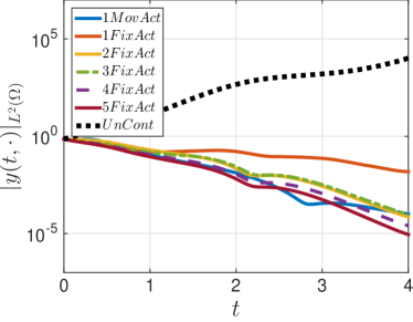
(a) $L^{2}(\Omega)$-norm for states

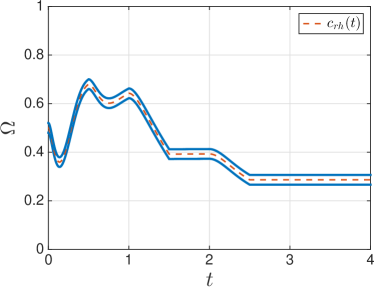
(b) Control domain movements

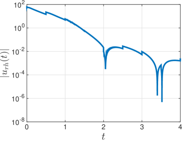
(c) Absolute value of magnitude

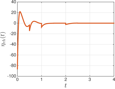
(d) Force

Figure 3. Example 5.1: Numerical results for $\beta=0.1$.

As can be seen from Figure 4(a), it is not clear for the case $\beta=0.5$ that one fixed actuator is asymptotically stabilizing. Moreover, for $M=4,5$ we have better stabilization results compared to the single moving control. Figures 3(b) and 4(b) illustrate the time evolution of the control domain $\omega(c_{rh}(t))$. From Figures 3(b), we can observe that, at some point ($t=2.5$), the actuator stops moving. This corresponds to Figure 3(d), which demonstrates the evolution of the force. In this case, the receding horizon framework moved the actuator until some degree of stabilization $(|y_{rh}(t,\raisebox{-1.07639pt}{\scalebox{1.25}{$\cdot$}})|_{L^{2}(\Omega)}\leq 10^{-3})$ was reached and, then, decided to steer the system with only a fixed actuator. In this case, the $|y_{rh}(t,\raisebox{-1.07639pt}{\scalebox{1.25}{$\cdot$}})|_{L^{2}(\Omega)}$-norm corresponding to $M=4$ and $M=5$ is smaller than the one corresponding to the single actuator which is free to move, once $t\geq 3$, see Figure 3(a). For the case $\beta=0.5$, we have a different scenario. In this case, the control remains moving throughout the whole simulation (see Figure 4(b)). This fact can also be seen from Figure  4(d) which shows that, here a stronger force was needed compared to the case $\beta=0.1$. Figures 3(c) and  4(c) show the evolution of the absolute value of the magnitude control $u_{rh}$.

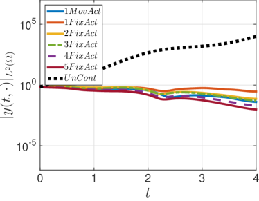
(a) $L^{2}(\Omega)$-norm for states

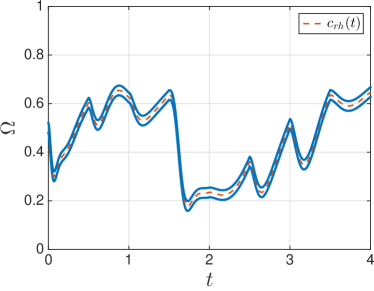
(b) Control domain movements

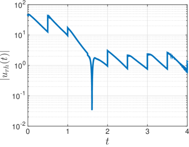
(c) Absolute value of magnitude

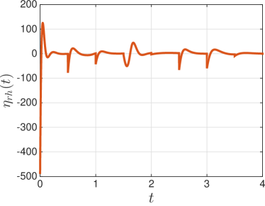
(d) Force

Figure 4. Example 5.1: Numerical results for $\beta=0.5$

Example 5.2.

Note that Proposition 1.2 implies says that if $y_{0}$ is an eigenfunction associated to a negative eigenvalue of ${\mathcal{A}}=-\nu\Delta-5{\mathbf{1}}$ and orthogonal to the fixed actuator, then the solution cannot be stabilized to zero. We present an example illustrating such a situation. A moving control steers, however, the system to zero. Here we used the same setting as in the previous example, except that we put

$$a(t,x) =-5,\quad b(t,x) =0,\quad y_{0}(x) =\sin(2\pi x).$$ (5.5a)

Finally, we take a fixed actuator $1_{\omega}$ centered at $0.5$,

$$\omega=(-\tfrac{r}{2},\tfrac{r}{2}).$$ (5.5b)

Clearly we have that $(y_{0},1_{\omega})_{L^{2}(\Omega)}=0$, and that $y_{0}$ is an eigenfunction of $-\nu\Delta-5{\mathbf{1}}$ with eigenvalue $4\pi^{2}\nu-5<0$. Thus we cannot stabilize the corresponding solution to zero. This is confirmed in Figure 5(a), where we can see that the single fixed actuator is not able to stabilize the system.

Furthermore, we can see that the curves corresponding to the uncontrolled state and one single fixed actuator are overlapping each other completely. This is not surprising, because $u^{*}=0$ is necessarily the unique minimum for all finite horizon open-loop problems with $y_{0}\in{\mathbb{R}}\sin(2\pi x)$. This is due to the fact that $(y_{0},1_{\omega})_{L^{2}(\Omega)}=0$.

On the other hand, we can see from Figures 5(b) and 5(a) that a single moving control is able to steer the system exponentially to zero by moving the actuator. Figures 5(c) and 5(d) depict the evolution of the absolute value of the magnitude $u_{rh}$ and the evolution of the force $\eta_{rh}$, respectively.

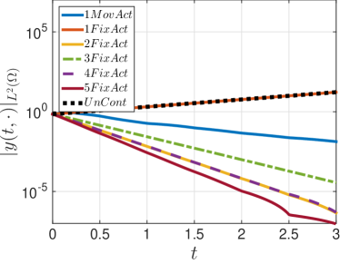
(a) $L^{2}(\Omega)$-norm for states

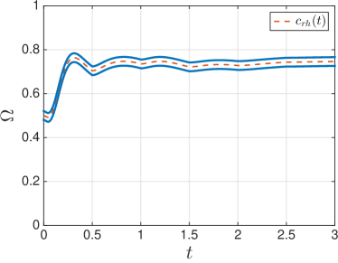
(b) Control domain movements

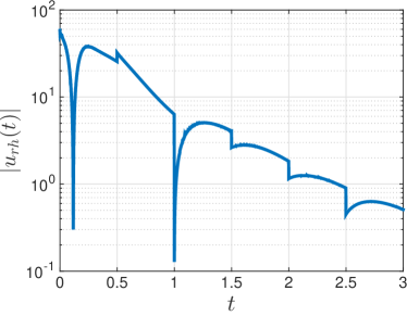
(c) Absolute value of magnitude

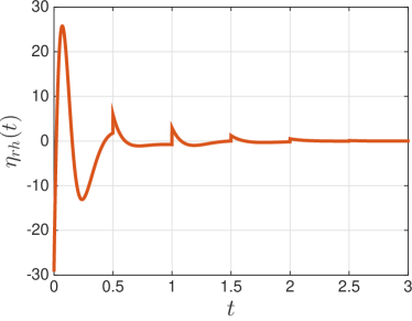
(d) Force

Figure 5. Example 5.2: Numerical results for $\beta=0.01$

Remark 5.3.

Note that, though the setting (5.5) serves to illustrate the orthogonality setting $(y_{0},1_{\omega})_{L^{2}(\Omega)}$ in Proposition 1.2, we can show that, in our 1D setting there are choices of $\omega$ which are able to stabilize the system. Indeed, all the eigenvalues are simple and for an actuator $1_{\omega}$ with $\omega=(a,b)\subseteq(0,1)$ we find that

$$(\sin(j\pi x),1_{\omega})_{L^{2}(\Omega)}=\tfrac{1}{j\pi}(\cos(j\pi a)-\cos(j\pi b)),\qquad j\in{\mathbb{N}}_{0}.$$

Hence, since

$$(\sin(j\pi x),1_{\omega})_{L^{2}(\Omega)}=0\Longleftrightarrow j\pi a\pm j\pi b\in\pm 2\pi{\mathbb{N}}\Longleftrightarrow j(a\pm b)\in\pm 2{\mathbb{N}},$$

we have that

$$(\sin(j\pi x),1_{\omega})_{L^{2}(\Omega)}\neq 0,\quad\mbox{for all}\quad j\in{\mathbb{N}}_{0},\quad\mbox{if}\quad\{a+b,a-b\}\subset{\mathbb{R}}\setminus{\mathbb{Q}},$$

where ${\mathbb{Q}}$ stands for the set of rational numbers. Therefore, by Proposition 1.3, we can stabilize the system if we replace $\omega$ in (5.5) by, for example, $\widetilde{\omega}=(-\frac{r}{2}-\varrho_{1},\frac{r}{2}+\varrho_{2})\subset(0,1)$ with $\{\varrho_{2}-\varrho_{1},r+\varrho_{2}+\varrho_{1}\}\subset{\mathbb{R}}\setminus{\mathbb{Q}}$. In particular taking small $\varrho_{1}\geq 0$ and small $\varrho_{2}\geq 0$ we see that with suitable arbitrary small perturbations $\widetilde{\omega}$ of $\omega$, the actuator $1_{\widetilde{\omega}}$ allows us stabilize the system.

Finally, notice that in 2D (which we do not consider here), for the unit square as spatial domain $\Omega$, the eigenvalues are not all simple and it will be always possible to find examples where a fixed actuator is not enough for stabilization (again, due to Proposition 1.2).

5.3. Remarks on the computation of the moving actuator

Summarizing, we can assert that the single moving actuator obtained by Algorithm 1 is able to stabilize the system to zero, confirming our theoretical findings.

For simplicity, and since the paper is already relatively long, we have restricted the numerical results to the 1D case.

The discretization of the optimal control problems in the 2D case is also more involved (due essentially to the adjoint equations). The 2D case will be addressed in a future work, where we plan to include also more details concerning the numerical realization. In particular, we plan to investigate the asymptotic stability of RHC and well-posedness of the associated finite-horizon open-loop subproblems.

It could also be of interest to investigate is the dependence on the stabilizability in the forcing bound parameter $K$. Here in our simulations we have chosen $K=500$ rather large, and the bound is never reached. It would be interesting to observe what happen when the bound is reached/active.

Appendix

A.4. Proofs of Propositions 1.2 and 1.3

Recall system (1.8),

$$\tfrac{\partial}{\partial t}y(t,x)-\nu\Delta y(t,x)+a(x)y(t,x)=u(t)\Psi,$$ (A.1a)

$$y(0,\raisebox{-1.07639pt}{\scalebox{1.25}{$\cdot$}})=y_{0},\qquad{\mathcal{G}}y\left.\kern-2.4pt\right|_{\Gamma}=0,$$ (A.1b)

and the system of eigenfunctions $\widetilde{e}_{i}$ and increasing sequence of eigenvalues $\widetilde{\alpha}_{i}$ of the operator ${\mathcal{A}}=-\nu\Delta+a(x){\mathbf{1}}$, ${\mathcal{A}}\widetilde{e}_{i}=\widetilde{\alpha}_{i}\widetilde{e}_{i}$.

We start with the following auxiliary result.

Lemma A.1.

If there exists a nonsimple eigenvalue $\widetilde{\alpha}_{j}$, then there exists one associated eigenfunction $\overline{e}_{j}$ such that $(\overline{e}_{j},\Psi)_{L^{2}(\Omega}=0$.

Proof.

If $\widetilde{\alpha}_{j}$ is a nonsimple eigenvalue, we can assume that $\widetilde{\alpha}_{j}=\widetilde{\alpha}_{j+1}$. Then, in case $(\widetilde{e}_{j},\Psi)_{L^{2}(\Omega)}=0$ or $(\widetilde{e}_{j+1},\Psi)_{L^{2}(\Omega)}=0$ the proof is finished. It remains to consider the case $(\widetilde{e}_{j},\Psi)_{L^{2}(\Omega}\eqqcolon\beta_{j}\neq 0\neq\beta_{j+1}\coloneqq(\widetilde{e}_{j+1},\Psi)_{L^{2}(\Omega}$. In this case we simply take the eigenfunction $\overline{e}_{j}\coloneqq\beta_{j+1}\widetilde{e}_{j}-\beta_{j}\widetilde{e}_{j+1}$ which satisfies $(\overline{e}_{j},\Psi)_{L^{2}(\Omega)}=\beta_{j+1}\beta_{j}-\beta_{j}\beta_{j+1}=0$. ∎

Proof of Proposition 1.2.

We take the eigenfunction given by Lemma A.1 as initial condition, $y_{0}\coloneqq\overline{e}_{j}$, $(\overline{e}_{j},\Psi)_{L^{2}(\Omega}=0$. By decomposing the solution into orthogonal components $y=q+Q$, with $q\in\mathop{\rm span}\nolimits\{\overline{e}_{j}\}$ and $Q\in\{\overline{e}_{j}\}^{\perp}$, we obtain

$$\tfrac{\partial}{\partial t}q(t,x)+{\mathcal{A}}q(t,x)=0, q(0)=\overline{e}_{j},$$ (A.2a)

$$\tfrac{\partial}{\partial t}Q(t,x)+{\mathcal{A}}Q(t,x)=u(t)\Psi, Q(0)=0,$$ (A.2b)

$${\mathcal{G}}q\left.\kern-2.4pt\right|_{\Gamma}=0={\mathcal{G}}Q\left.\kern-2.4pt\right|_{\Gamma}.$$ (A.2c)

Observe that the dynamics of the component $q$ is independent of $u$, and such component is then given by $q(t,\raisebox{-1.07639pt}{\scalebox{1.25}{$\cdot$}})={\mathrm{e}}^{-\widetilde{\alpha}_{j}t}\overline{e}_{j}$, $t>0$. Now, for the norm of the entire state we obtain

$$\left|y(t,\raisebox{-1.07639pt}{\scalebox{1.25}{$\cdot$}})\right|_{L^{2}(\Omega)}^{2}=\left|q(t,\raisebox{-1.07639pt}{\scalebox{1.25}{$\cdot$}})\right|_{L^{2}(\Omega)}^{2}+\left|Q(t,\raisebox{-1.07639pt}{\scalebox{1.25}{$\cdot$}})\right|_{L^{2}(\Omega)}^{2}\geq{\mathrm{e}}^{-2\widetilde{\alpha}_{j}t}\left|\overline{e}_{j}\right|_{L^{2}(\Omega)}^{2},\qquad t>0,$$

for every magnitude control $u$. ∎

Proof of Proposition 1.3.

Let $j_{0}\coloneqq\min\{j\in{\mathbb{N}}\mid\widetilde{\alpha}_{j}>0\}$. If $j_{0}=1$ then the free dynamics is exponentially stable. If $j_{0}>1$, then we consider the dynamics onto the linear span of the first $j_{0}-1$ eigenfunctions

$${\mathcal{E}}_{j_{0}-1}\coloneqq\mathop{\rm span}\nolimits\{\widetilde{e}_{j}\mid 1\leq j\leq j_{0}-1\},\qquad q(t)\coloneqq P_{{\mathcal{E}}_{j_{0}-1}}y(t)\in{\mathcal{E}}_{j_{0}-1}$$

where $P_{{\mathcal{E}}_{j_{0}-1}}\in{\mathcal{L}}(L^{2}(\Omega),{\mathcal{E}}_{j_{0}-1})$ denotes the orthogonal projection in $L^{2}(\Omega)$ onto the subspace ${\mathcal{E}}_{j_{0}-1}$. We decompose the system as

$$\tfrac{\partial}{\partial t}q(t,x)+{\mathcal{A}}q(t,x)=u(t)P_{{\mathcal{E}}_{j_{0}-1}}\Psi, q(0)=P_{{\mathcal{E}}_{j_{0}-1}}y_{0},$$ (A.3a)

$$\tfrac{\partial}{\partial t}Q(t,x)+{\mathcal{A}}Q(t,x)=u(t)P_{{\mathcal{E}}_{j_{0}-1}^{\perp}}\Psi, Q(0)=P_{{\mathcal{E}}_{j_{0}-1}^{\perp}}y_{0},$$ (A.3b)

$${\mathcal{G}}q\left.\kern-2.4pt\right|_{\Gamma}=0={\mathcal{G}}Q\left.\kern-2.4pt\right|_{\Gamma},$$ (A.3c)

with $Q=y-q=P_{{\mathcal{E}}_{j_{0}-1}^{\perp}}y$. Next we prove that the finite dimensional system (A.3a) is null controllable. Writing

$$q=\textstyle\sum\limits_{k=1}^{j_{0}-1}q_{k}\widetilde{e}_{k},\qquad\overline{q}=\begin{bmatrix}q_{1}\\ q_{2}\\ \vdots\\ q_{j_{0}-1}\end{bmatrix}$$

we obtain the system

$$\dot{\overline{q}}=A\overline{q}+Bu,$$ (A.4)

with $A\in{\mathbb{R}}^{(j_{0}-1)\times(j_{0}-1)}$ and $B\in{\mathbb{R}}^{(j_{0}-1)\times 1}$ as follows

$$A={\rm diag}\left(\widetilde{\alpha}_{1},\widetilde{\alpha}_{2},\dots,\widetilde{\alpha}_{j_{0}-1}\right)\quad\mbox{and}\quad B=\begin{bmatrix}(\widetilde{e}_{1},\Psi)\\ (\widetilde{e}_{2},\Psi)\\ \vdots\\ (\widetilde{e}_{j_{0}-1},\Psi)\end{bmatrix}.$$

The matrix $A$ is diagonal with entries $A_{(i,i)}=\widetilde{\alpha}_{i}$.

For any given $T>0$, we have that system (A.4) is controllable at time $T$. Indeed, this follows from Kalman rank condition (see, e.g., [32, Sect 1.3, Thm. 1.2]), because we have that

$$\det(\begin{bmatrix}A\mid B\end{bmatrix})=\left(\bigtimes_{k=1}^{j_{0}-1}(\widetilde{e}_{k},\Psi)\right)\det{\mathcal{V}}$$

where

$$\begin{bmatrix}A\mid B\end{bmatrix}\coloneqq\begin{bmatrix}B&AB&\dots&A^{j_{0}-2}B\end{bmatrix}$$

and ${\mathcal{V}}$ is the Vandermonde matrix whose entries are

$${\mathcal{V}}_{(i,j)}=\widetilde{\alpha}_{i}^{j-1}.$$

Hence

$$\det(\begin{bmatrix}A\mid B\end{bmatrix})=\left(\bigtimes_{k=1}^{j_{0}-1}(\widetilde{e}_{k},\Psi)\right)\left(\bigtimes_{1\leq i<j\leq j_{0}-1}(\widetilde{\alpha}_{j}-\widetilde{\alpha}_{i})\right)\neq 0.$$

Therefore, we can choose a control $u$ such that $\overline{q}(T,\raisebox{-1.07639pt}{\scalebox{1.25}{$\cdot$}})=0$, which implies $q(T,\raisebox{-1.07639pt}{\scalebox{1.25}{$\cdot$}})=0$. Then, we take the concatenated control defined as: $u^{c}(t)$ if $t\in[0,T]$, and $u^{c}(t)=0$ for $t>T$. For time $t\geq T$ we have that $q(t,\raisebox{-1.07639pt}{\scalebox{1.25}{$\cdot$}})=0$ and

$$\left|y(t,\raisebox{-1.07639pt}{\scalebox{1.25}{$\cdot$}})\right|_{L^{2}(\Omega)}^{2}=\left|Q(t,\raisebox{-1.07639pt}{\scalebox{1.25}{$\cdot$}})\right|_{L^{2}(\Omega)}^{2}={\mathrm{e}}^{-\widetilde{\alpha}_{j_{0}}(t-T)}\left|Q(T,\raisebox{-1.07639pt}{\scalebox{1.25}{$\cdot$}})\right|_{L^{2}(\Omega)},\qquad t\geq T.$$

Since, by definition of $j_{0}$, we have that $\widetilde{\alpha}_{j_{0}}>0$, it follows that $\left|y(t,\raisebox{-1.07639pt}{\scalebox{1.25}{$\cdot$}})\right|_{L^{2}(\Omega)}^{2}$ converges exponentially to zero, as $t\to+\infty$. That is, $u^{c}$ is a stabilizing (open-loop) control. ∎

The proofs of Propositions 1.2 and 1.3 above are quite intuitive for the considered concrete system. Shorter proofs would follow from applications of the Fattorini criterium for stability that we find for example in [6]. At this point we would like to refer the reader also to the work by Hautus in [15, Sect. 3] for further comments on controllability and stabilizability of more general finite-dimensional autonomous systems (including both continuous-time and discrete-time cases). See also [31, Sect. 6.5] for a version of the Hautus test for the observability of linear abstract infinite-dimensional systems (here recall also the duality between observability and controllability).

A.5. Proof of Proposition 3.4.

Let us fix an arbitrary $\delta>0$ and let $h\in{\mathfrak{S}}_{H}$ be in the unit ball of $H$. Since $X$ is dense in $H$, we can choose $\overline{h}\in X\setminus\{0\}$ such that $\left|\overline{h}-h\right|_{H}\leq\frac{\delta}{2}$. Now, for $\widetilde{h}\coloneqq\left|\overline{h}\right|_{H}^{-1}\overline{h}\in{\mathfrak{S}}_{H}$ we find

$$\left|\widetilde{h}-h\right|_{H} \leq\left|\left|\overline{h}\right|_{H}^{-1}\overline{h}-\overline{h}\right|_{H}+\left|\overline{h}-h\right|_{H}\leq\left|\left|\overline{h}\right|_{H}^{-1}-1\right|_{{\mathbb{R}}}\left|\overline{h}\right|_{H}+\tfrac{\delta}{2}$$

$$=\left|\overline{h}\right|_{H}^{-1}\left|1-\left|\overline{h}\right|_{H}\right|_{{\mathbb{R}}}\left|\overline{h}\right|_{H}+\tfrac{\delta}{2}=\left|\left|h\right|_{H}-\left|\overline{h}\right|_{H}\right|_{{\mathbb{R}}}+\tfrac{\delta}{2}\leq\left|h-\overline{h}\right|_{H}+\tfrac{\delta}{2}=\delta.$$

Hence we can conclude that $X\bigcap{\mathfrak{S}}_{H}$ is dense in ${\mathfrak{S}}_{H}$. ∎

A.6. Proof of Proposition 3.6

We start by defining

$$\overline{t}_{j}\coloneqq\max\{\tau_{j},\sigma_{j}\},\qquad\underline{t}_{j}\coloneqq\min\{\tau_{j},\sigma_{j}\},\qquad 0\leq j\leq K,$$

and by writing, with $g\coloneqq f_{\tau}-f_{\sigma}$,

$$\left|f_{\tau}-f_{\sigma}\right|_{L^{2}((a,b),X)}^{2}=\sum_{j=1}^{K}\int_{\overline{t}_{j-1}}^{\overline{t}_{j}}\left|f_{\tau}(t)-f_{\sigma}(t)\right|_{X}^{2}\,\mathrm{d}t=\sum_{j=1}^{K}\int_{\overline{t}_{j-1}}^{\overline{t}_{j}}\left|g(t)\right|_{X}^{2}\,\mathrm{d}t.$$ (A.5)

We proceed by Induction. Firstly, we find that

$$\int_{a}^{\overline{t}_{1}}\left|g(t)\right|_{X}^{2}\,\mathrm{d}t =\int_{\overline{t}_{0}}^{\overline{t}_{1}}\left|g(t)\right|_{X}^{2}\,\mathrm{d}t=\int_{\underline{t}_{1}}^{\overline{t}_{1}}\left|g(t)\right|_{X}^{2}\,\mathrm{d}t\leq{\mathcal{R}}{\mathcal{X}}^{2},$$ (A.6)

where in the last inequality we used the fact that $g(t)=f_{\tau}(t)-f_{\sigma}(t)=\phi_{1}-\phi_{1}=0$ for $t\in[\overline{t}_{0},\underline{t}_{1})$.

Next, we assume that for a given $i\in\{1,2,\dots,K-1\}$ we have

$$\int_{a}^{\overline{t}_{i}}\left|g(t)\right|_{X}^{2}\,\mathrm{d}t\leq i{\mathcal{R}}{\mathcal{X}}^{2}. {\mathfrak{H}}$$ ()

Then we obtain

$$\int_{a}^{\overline{t}_{i+1}}\left|g(t)\right|_{X}^{2}\,\mathrm{d}t \leq i{\mathcal{R}}{\mathcal{X}}^{2}+\int_{\overline{t}_{i}}^{\overline{t}_{i+1}}\left|g(t)\right|_{X}^{2}\,\mathrm{d}t,$$

which implies that

$$\int_{a}^{\overline{t}_{i+1}}\left|g(t)\right|_{X}^{2}\,\mathrm{d}t \leq i{\mathcal{R}}{\mathcal{X}}^{2}+\int_{\overline{t}_{i}}^{\underline{t}_{i+1}}\left|g(t)\right|_{X}^{2}\,\mathrm{d}t+\int_{\underline{t}_{i+1}}^{\overline{t}_{i+1}}\left|g(t)\right|_{X}^{2}\,\mathrm{d}t,\quad\mbox{if}\quad\overline{t}_{i}<\underline{t}_{i+1}\leq\overline{t}_{i+1},$$

and

$$\int_{a}^{\overline{t}_{i+1}}\left|g(t)\right|_{X}^{2}\,\mathrm{d}t \leq i{\mathcal{R}}{\mathcal{X}}^{2}+\int_{\underline{t}_{i+1}}^{\overline{t}_{i+1}}\left|g(t)\right|_{X}^{2}\,\mathrm{d}t,\quad\mbox{if}\quad\underline{t}_{i+1}\leq\overline{t}_{i}\leq\overline{t}_{i+1},$$

Observe that, if $\overline{t}_{i}<\underline{t}_{i+1}$, then $g(t)=f_{\tau}(t)-f_{\sigma}(t)=\phi_{i+1}-\phi_{i+1}=0$, for $t\in(\overline{t}_{i},\underline{t}_{i+1})\subseteq(\tau_{i},\tau_{i+1})\bigcap(\sigma_{i},\sigma_{i+1})$. Therefore, in either case we have

$$\int_{a}^{\overline{t}_{i+1}}\left|g(t)\right|_{X}^{2}\,\mathrm{d}t \leq i{\mathcal{R}}{\mathcal{X}}^{2}+\int_{\underline{t}_{i+1}}^{\overline{t}_{i+1}}\left|g(t)\right|_{X}^{2}\,\mathrm{d}t\leq i{\mathcal{R}}{\mathcal{X}}^{2}+{\mathcal{R}}{\mathcal{X}}^{2}=(i+1){\mathcal{R}}{\mathcal{X}}^{2}. {\mathfrak{T}}$$ ()

Hence, assumption (${\mathfrak{H}}$) implies (${\mathfrak{T}}$), which together with (A.6) imply, by Induction,

$$\int_{a}^{\overline{t}_{j}}\left|g(t)\right|_{X}^{2}\,\mathrm{d}t\leq j{\mathcal{R}}{\mathcal{X}}^{2},\quad\mbox{for all}\quad j\in\{1,2,\dots,K\}.$$ (A.7)

In particular, since $\overline{t}_{K}=b$, for $j=K$ we obtain $\left|f_{\tau}-f_{\sigma}\right|_{L^{2}((a,b),X)}\leq K^{\frac{1}{2}}{\mathcal{R}}^{\frac{1}{2}}{\mathcal{X}}$. ∎

Acknowledgments. K. Kunisch was supported in part by the ERC advanced grant 668998 (OCLOC) under the EU’s H2020 research program. S. Rodrigues gratefully acknowledges partial support from the Austrian Science Fund (FWF): P 33432-NBL.

References

- [1] A. A. Agrachev and A. V. Sarychev. Navier–Stokes equations: Controllability by means of low modes forcing. J. Math. Fluid Mech., 7(1):108–152, 2005. doi:10.1007/s00021-004-0110-1.
- [2] A. A. Agrachev and A. V. Sarychev. Controllability of 2D Euler and Navier–Stokes equations by degenerate forcing. Commun. Math. Phys., 265(3):673–697, 2006. doi:10.1007/s00220-006-0002-8.
- [3] B. Azmi and K. Kunisch. A hybrid finite-dimensional RHC for stabilization of time-varying parabolic equations. SIAM J. Control Optim., 57(5):3496–3526, 2019. doi:10.1137/19M1239787.
- [4] B. Azmi and K. Kunisch. Analysis of the Barzilai-Borwein step-sizes for problems in Hilbert spaces. J. Optim. Theory Appl., 185(3):819–844, 2020. doi:10.1007/s10957-020-01677-y.
- [5] M. Badra. Feedback stabilization of the 2-D and 3-D Navier–Stokes equations based on an extended system. ESAIM Control Optim. Calc. Var., 15(4):934–968, 2009. doi:10.1051/cocv:2008059.
- [6] M. Badra and T. Takahashi. On the Fattorini criterion for approximate controllability and stabilizability of parabolic systems. ESAIM Control Optim. Calc. Var., 20:924–956, 2014. doi:10.1051/cocv/2014002.
- [7] J. Barzilai and J. M. Borwein. Two-point step size gradient methods. IMA J. Numer. Anal., 8(1):141–148, 1988. doi:10.1093/imanum/8.1.141.
- [8] T. Breiten, K. Kunisch, and S. S. Rodrigues. Feedback stabilization to nonstationary solutions of a class of reaction diffusion equations of FitzHugh–Nagumo type. SIAM J. Control Optim., 55(4):2684–2713, 2017. doi:10.1137/15M1038165.
- [9] C. Castro, N. Cîndea, and A. Münch. Controllability of the linear one-dimensional wave equation with inner moving forces. SIAM J. Control Optim., 52(6):4027–4056, 2014. doi:10.1137/140956129.
- [10] C. Castro and E. Zuazua. Unique continuation and control for the heat equation from an oscillating lower dimensional manifold. SIAM J. Control Optim., 43(4):1400–1434, 2005. doi:10.1137/S0363012903430317.
- [11] F. W. Chaves-Silva, L. Rosier, and E. Zuazua. Null controllability of a system of viscoelasticity with a moving control. J. Math. Pures Appl., 101(2):198–222, 2014. doi:10.1016/j.matpur.2013.05.009.
- [12] Yu-H. Dai and R. Fletcher. New algorithms for singly linearly constrained quadratic programs subject to lower and upper bounds. Math. Program., 106(3, Ser. A):403–421, 2006. doi:10.1007/s10107-005-0595-2.
- [13] M. A. Demetriou. Guidance of mobile actuator-plus-sensor networks for improved control and estimation of distributed parameter systems. IEEE Trans. Automat. Control, 55(7):1570–1584, 2010. doi:10.1109/TAC.2010.2042229.
- [14] R. V. Gamkrelidze. Principles of Optimal Control Theory. Plenum Press, 1978. doi:10.1007/978-1-4684-7398-8.
- [15] M. L. J. Hautus. Stabilization controllability and observability of linear autonomous systems. Indag. Math. (Proceedings), 73:448–455, 1970. doi:10.1016/S1385-7258(70)80049-X.
- [16] Y. He. Two-level method based on finite element and Crank-Nicolson extrapolation for the time-dependent Navier-Stokes equations. SIAM J. Numer. Anal., 41(4):1263–1285, 2003. doi:10.1137/S0036142901385659.
- [17] M. Hintermüller and K. Kunisch. Path-following methods for a class of constrained minimization problems in function space. SIAM J. Optim., 17(1):159–187, 2006. doi:10.1137/040611598.
- [18] A. Khapalov. -exact observability of the heat equation with scanning pointwise sensor. SIAM J. Control Optim., 32(4):1037–1051, 1994. doi:10.1137/S036301299222737X.
- [19] A. Khapalov. Approximate controllability and its well-posedness for the semilinear reaction-diffusion equation with internal lumped controls. ESAIM Control, Optim. Calc. Var., 4:83–98, 1999. doi:10.1051/cocv:1999104.
- [20] A. Khapalov. Mobile point controls versus locally distributed ones for the controllability of the semilinear parabolic equation. SIAM J. Control Optim., 40(1):231–252, 2001. doi:10.1137/S0363012999358038.
- [21] K. Kunisch and S. S. Rodrigues. Explicit exponential stabilization of nonautonomous linear parabolic-like systems by a finite number of internal actuators. ESAIM Control Optim. Calc. Var., 2018. doi:10.1051/cocv/2018054.
- [22] K. Kunisch and D. A Souza. On the one-dimensional nonlinear monodomain equations with moving controls. J. Math. Pures Appl., 117:94–122, 2018. doi:10.1016/j.matpur.2018.05.003.
- [23] Ph. Martin, L. Rosier, and P. Rouchon. Null controllability of the structurally damped wave equation with moving control. SIAM J. Control Optim., 51(1):660–684, 2013. doi:10.1137/110856150.
- [24] D. Phan and S. S. Rodrigues. Stabilization to trajectories for parabolic equations. Math. Control Signals Syst., 30(2):11, 2018. doi:10.1007/s00498-018-0218-0.
- [25] S. S. Rodrigues. Navier–Stokes equation on the Rectangle: Controllability by means of low modes forcing. J. Dyn. Control Syst., 12(4):517–562, 2006. doi:10.1007/s10883-006-0004-z.
- [26] S. S. Rodrigues. Methods of Geometric Control Theory in Problems of Mathematical Physics. PhD Thesis. Universidade de Aveiro, Portugal, 2008. URL: http://hdl.handle.net/10773/2931.
- [27] S. S. Rodrigues. Feedback boundary stabilization to trajectories for 3D Navier–Stokes equations. Appl. Math. Optim., 2018. doi:10.1007/s00245-017-9474-5.
- [28] S. S. Rodrigues. Semiglobal exponential stabilization of nonautonomous semilinear parabolic-like systems. Evol. Equ. Control Theory, 9(3):635–672, 2020. doi:10.3934/eect.2020027.
- [29] S. S. Rodrigues and K. Sturm. On the explicit feedback stabilization of one-dimensional linear nonautonomous parabolic equations via oblique projections. IMA J. Math. Control Inform., 37(1):175–207, 2020. doi:10.1093/imamci/dny045.
- [30] A. Shirikyan. Exact controllability in projections for three-dimensional Navier–Stokes equations. Ann. Inst. H. Poincaré Anal. Non Linéaire, 24(4):521–537, 2007. doi:10.1016/j.anihpc.2006.04.002.
- [31] M. Tucsnak and G. Weiss. Observation and Control for Operator Semigroups. Birkhäuser Basel, Basel, 2009. doi:10.1007/978-3-7643-8994-9.
- [32] J. Zabczyk. Mathematical Control Theory: an Introduction. Systems Control Found. Appl. Birkhäuser, Boston, 1992. doi:10.1007/978-0-8176-4733-9.