Magellanic satellites in $\Lambda$CDM cosmological hydrodynamical simulations of the Local Group

Abstract

We use the APOSTLE $\Lambda$CDM cosmological hydrodynamical simulations of the Local Group to study the recent accretion of massive satellites into the halo of Milky Way (MW)-sized galaxies. These systems are selected to be close analogues to the Large Magellanic Cloud (LMC), the most massive satellite of the MW. The simulations allow us to address, in a cosmological context, the impact of the Clouds on the MW, including the contribution of Magellanic satellites to the MW satellite population, and the constraints placed on the Galactic potential by the motion of the LMC. We show that LMC-like satellites are twice more common around Local Group-like primaries than around isolated halos of similar mass; these satellites come from large turnaround radii and are on highly eccentric orbits whose velocities at first pericentre are comparable with the primary’s escape velocity. This implies $V_{\rm esc}^{\rm MW}(50$ kpc$)\sim 365$ km/s, a strong constraint on Galactic potential models. LMC analogues contribute about 2 satellites with $M_{*}>10^{5}\,M_{\odot}$, having thus only a mild impact on the luminous satellite population of their hosts. At first pericentre, LMC-associated satellites are close to the LMC in position and velocity, and are distributed along the LMC’s orbital plane. Their orbital angular momenta roughly align with the LMC’s, but, interestingly, they may appear to “counter-rotate” the MW in some cases. These criteria refine earlier estimates of the LMC association of MW satellites: only the SMC, Hydrus1, Car3, Hor1, Tuc4, Ret2 and Phoenix2 are compatible with all criteria. Carina, Grus2, Hor2 and Fornax are less probable associates given their large LMC relative velocity.

1 Introduction

It is now widely agreed that the Large Magellanic Cloud (LMC), the most luminous satellite of the Milky Way (MW), is at a particular stage of its orbit. Its large Galactocentric velocity ($\sim 328$ km/s) is dominated by the tangential component ($\sim 320$ km/s) and is much higher than all plausible estimates of the MW circular velocity at its present distance of $\sim 50$ kpc (see; e.g., Kallivayalil et al., 2013; Gaia Collaboration et al., 2018, and references therein). This implies that the LMC is close to the pericentre of a highly eccentric orbit with large apocentric distance and long orbital times. Together with the presence of a clearly asociated close companion (the Small Magellanic Cloud, SMC, see; e.g., Westerlund, 1990; D’Onghia & Fox, 2016), the evidence strongly suggests that the Clouds are just past their first closest approach to the Galaxy (Besla et al., 2007; Boylan-Kolchin et al., 2011; Patel et al., 2017a).

The particular kinematic stage of the LMC, together with the relatively high stellar mass of the Clouds ($M_{*}\sim 2.5\times 10^{9}\,M_{\odot}$; Kim et al., 1998), offer clues about the MW virial mass and insight into the hierarchical nature of galaxy clustering in the dwarf galaxy regime.

Clues about the MW mass fall into two classes. One concerns the relation between virial mass and satellite statistics; namely, the more massive the Milky Way halo the higher the likelihood of hosting a satellite as massive as the LMC. Empirically, observational estimates suggest that up to $\sim 40\%$ of $L^{*}$ galaxies may host a satellite as luminous as the LMC within $\sim 250$ kpc and up to a $10\%$ chance of having one within $\sim 50$ kpc (Tollerud et al., 2011). This result has been interpreted as setting a lower limit on the MW virial mass of roughly $\sim 10^{12}$ M_⊙ (Busha et al., 2011; Boylan-Kolchin et al., 2011; Patel et al., 2017a; Shao et al., 2018).

The other class relates to kinematics; if the LMC is near its first pericentric passage, its velocity, not yet affected substantially by dynamical friction, should reflect the total acceleration experienced during its infall. If, as seems likely, that infall originated far from the MW virial boundary, then the LMC velocity would provide a robust estimate of the MW escape velocity at its present location. This assumes, of course, that the LMC is bound to the MW, an argument strongly supported by its status as the most luminous and, hence, most massive satellite. Unbound satellites are indeed possible, but they tend to occur during the tidal disruption of groups of dwarfs, and to affect only the least massive members of a group (see; e.g., Sales et al., 2007).

A strong constraint on the MW escape velocity at $r\sim 50$ kpc, $V^{\rm MW}_{\rm esc}$, could help to discriminate between competing Galactic potential models by adding information at a distance where other tracers are scarce and where commonly-used Galactic potential models often disagree (see; e.g., Irrgang et al., 2013; Bovy, 2015; Garavito-Camargo et al., 2019; Errani & Peñarrubia, 2020). For example, $V^{\rm MW}_{\rm esc}$ at $50$ kpc vary between $\sim 450$ km/s and $\sim 330$ km/s for the four Galactic models proposed in these references.

The peculiar kinematic state of the LMC adds complexity to the problem, but also offers unique opportunities. On the one hand, the short-lived nature of a first pericentric passage implies that the MW satellite population is in a transient state and out of dynamical equilibrium. This compromises the use of simple equilibrium equations to interpret the dynamics of the MW satellites, and reduces the usefulness of the MW satellites as a template against which the satellite populations of external galaxies may be contrasted.

However, it also offers a unique opportunity to study the satellites of the LMC itself. If on first approach, most LMC-associated dwarfs should still lie close to the LMC itself, as the Galactic tidal field would not have had time yet to disperse them (Sales et al., 2011). If we can disentangle the LMC satellite population from that of the MW then we can directly study the satellite population of a dwarf galaxy, with important applications to our ideas of hierarchical galaxy formation (D’Onghia & Lake, 2008) and to the relation between galaxy stellar mass and halo mass at the faint-end of the galaxy luminosity function (Sales et al., 2013).

The issue of which MW satellites are “Magellanic” in origin has been the subject of several recent studies, mainly predicated on the idea that LMC satellites should today have positions and velocities consistent with what is expected for the tidal debris of the LMC halo (Sales et al., 2011; Yozin & Bekki, 2015; Jethwa et al., 2016). One application of these ideas is that LMC satellites should accompany the LMC orbital motion and, therefore, should have orbital angular momenta roughly parallel to that of the LMC.

Using such dynamical premises, current estimates based on accurate proper motions from Gaia-DR2 have suggested at least four ultrafaint dwarfs (Car 2, Car 3, Hor 1, and Hydrus 1) as highly probable members of the LMC satellite system (Kallivayalil et al., 2018; Fritz et al., 2018), an argument supported and extended further by semianalytic modeling of the ultrafaint population (Dooley et al., 2017; Nadler et al., 2019).

Taking into account the combined gravitational potential of the MW+LMC system might bring two extra candidates (Phx 2 and Ret 2) into plausible association with the LMC (Erkal & Belokurov, 2020; Patel et al., 2020). Revised kinematics for the classical dwarfs have also led to suggestions that the Carina and Fornax dSph could have been brought in together with the LMC (Jahn et al., 2019; Pardy et al., 2020). Further progress requires refining and extending membership criteria in order to establish the identity of the true Magellanic satellites beyond doubt.

Much of the progress reported above has been made possible by LMC models based on tailored simulations where the Milky Way and the LMC are considered in isolation, or on dark matter-only cosmological simulations where luminous satellites are not explicitly followed. This paper aims at making progress on these issues by studying the properties of satellite systems analogous to the LMC identified in cosmological hydrodynamical simulations of Local Group environments from the APOSTLE project.

The paper is organized as follows. We describe our numerical datasets in Sec. 2, and the identification of LMC analogues in APOSTLE in Sec. 3. The satellites of such analogues, and their effect on the primary satellite population, are explored in Sec. 4. Finally, Sec. 5 uses these results to help identify Magellanic satellites in the MW and Sec. 6 considers the constraints placed by the LMC on the MW escape velocity and Galactic potential. We conclude with a brief summary in Sec. 7.

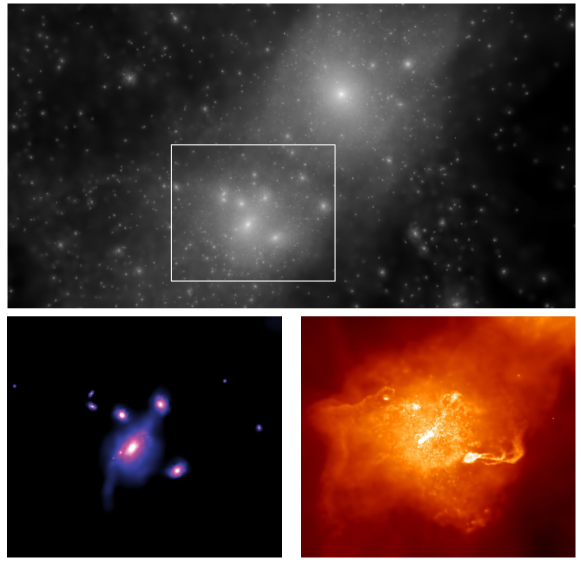
Figure 1: An image of an APOSTLE simulation volume that includes an LMC analogue as defined in this work (labelled 1-1-1 in subsequent figures and tables). The upper panel shows the dark matter distribution of the Local group-like environment, with the M31 analogue in the upper right part of the panel, and the MW analogue in the bottom left. The area enclosed in a rectangle, which includes the MW and LMC analogues, is shown in the bottom-left and bottom-right panels in stellar and gas density projections, respectively. The LMC analogue is the object located on the lower right in the bottom panels. Note the purely gaseous stream that emerges from it, with no stellar counterpart, reminiscent of a “Magellanic stream”.

2 Numerical Simulations

All simulations used in this paper adopt a flat $\Lambda$CDM model with parameters based on WMAP-7 (Komatsu et al., 2011): $\Omega_{\rm m}=0.272$, $\Omega_{\Lambda}=0.728$, $\Omega_{\rm bar}=0.0455$, $H_{0}=100\,h\,\,{\rm km\,s^{-1}}\,{\rm Mpc}^{-1}$, $\sigma=0.81$, with $h=0.704$.

2.1 The DOVE simulation

We use the DOVE cosmological N-body simulation to study the frequency of massive satellites around Milky Way-mass haloes and possible environmental effects in Local Group volumes. DOVE evolves a $100^{3}\,{\rm Mpc}^{3}$ cosmological box with periodic boundary conditions (Jenkins, 2013) with $1620^{3}$ collisionless particles with mass per particle $m_{\rm p}=8.8\times 10^{6}$ $\;\rm M_{\odot}$. The initial conditions for the box were made using panphasia (Jenkins, 2013) at $z=127$, and were evolved to $z=0$ using the Tree-PM code P-Gadget3, a modified version of the publicly available Gadget-2 (Springel, 2005).

2.2 The APOSTLE simulations

The APOSTLE project is a suite of “zoom-in” cosmological hydrodynamical simulations of twelve Local Group-like environments, selected from the DOVE box (Sawala et al., 2016). These Local Group volumes are defined by the presence of a pair of haloes whose masses, relative radial and tangential velocities, and surrounding Hubble flow match those of the Milky Way-Andromeda pair (see Fattahi et al., 2016, for details).

APOSTLE volumes have been run with the EAGLE (Evolution and Assembly of GaLaxies and their Environments) galaxy formation code (Schaye et al., 2015; Crain et al., 2015), which is a modified version of the Tree-PM SPH code P-Gadget3. The subgrid physics model includes radiative cooling, star formation in regions denser than a metallicity-dependent density threshold, stellar winds and supernovae feedback, homogeneous X-ray/UV background radiation, as well as supermassive black-hole growth and active galactic nuclei (AGN) feedback (the latter has substantive effects only on very massive galaxies and its effects are thus essentially negligible in APOSTLE volumes).

The model was calibrated to approximate the stellar mass function of galaxies at $z=0.1$ in the stellar mass range of $M_{\rm star}=10^{8}$-$10^{12}\,M_{\odot}$, and to yield realistic galaxy sizes. This calibration means that simulated galaxies follow fairly well the abundance-matching relation of Behroozi et al. (2013) or Moster et al. (2013) (see Schaye et al., 2015).

Although dwarf galaxy sizes were not used to adjust the model, they are nevertheless in fairly good agreement with observational data (Campbell et al., 2017). Isolated dwarf galaxies follow as well a tight $M_{\rm star}$-$V_{\rm max}$ relation (see Fig. 1 in Fattahi et al., 2018), consistent with extrapolations of abundance-matching models. The APOSTLE simulations have been run at three different levels of resolution, all using the "Reference" parameters of the EAGLE model. In this work we use the medium resolution runs (labelled “AP-L2”), with initial dark matter and gas particle masses of $m_{\rm dm}\sim 5.9\times 10^{6}\rm M_{\odot}$ and $m_{\rm gas}\sim 1.2\times 10^{5}\rm M_{\odot}$, respectively. As in DOVE, haloes and subhaloes in APOSTLE are identified using a friends-of-friends groupfinding algorithm (Davis et al., 1985) and subfind (Springel et al., 2001). These have been linked between snapshots by means of merger trees, which allow us to trace individual systems back in time (Qu et al., 2017).

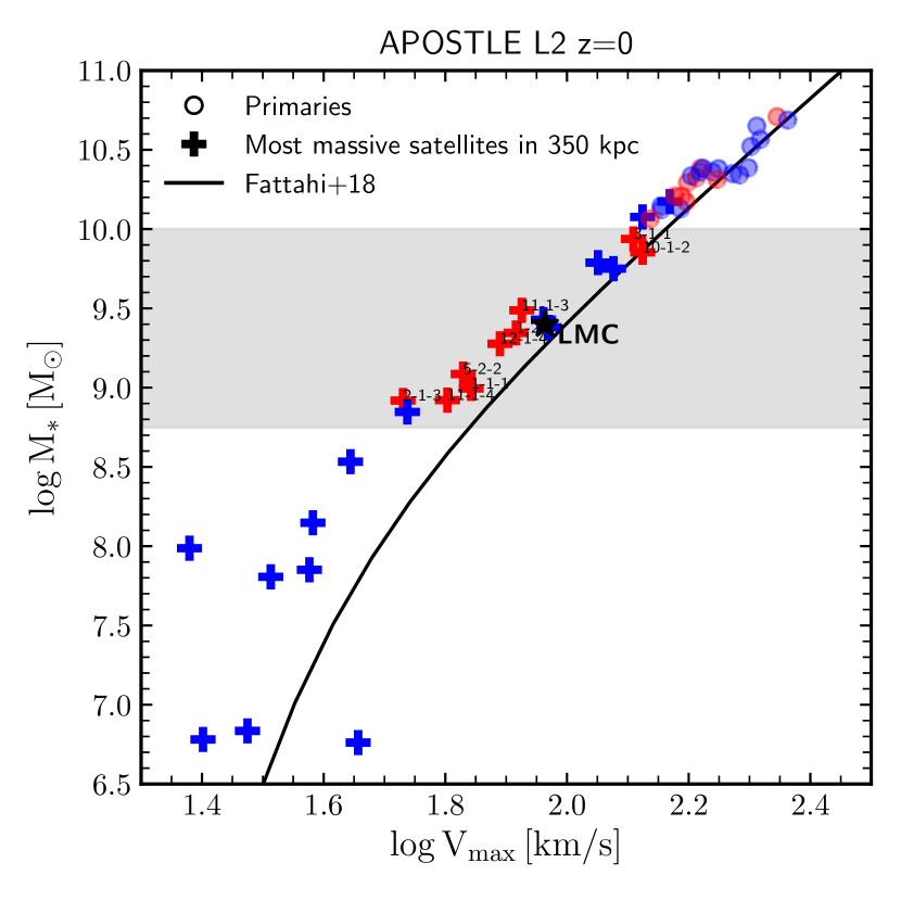
Figure 2: $V_{\rm max}$-$M_{*}$ relation for the most massive satellites (crosses) of the 24 primaries (circles; i.e., MW and M31 analogues) from the 12 APOSTLE-L2 volumes at $z=0$. The shaded area delimits the $M_{*}$ range around the LMC’s observed stellar mass value (star symbol) chosen to search for LMC-analogue candidates. The final LMC analogues that were selected for analysis in this work (see Sec. 3.2), and their corresponding primaries, are shown in red. A line shows the average $V_{\rm max}$-$M_{*}$ relation for APOSTLE centrals from Fattahi et al. (2018).

2.3 Galaxy identification

Particles in the simulations are grouped together using the friends-of-friends algorithm (FoF; Davis et al., 1985), with a linking length of $0.2$ times the mean inter-particle separation. Self-bound substructures within the FoF groups are identified using subfind (Springel et al., 2001). We refer to the most massive subhalo of a FoF group as “central” or “primary” and to the remainder as “satellites”.

APOSTLE galaxies and haloes are identified as bound structures, found by subfind within $3$ Mpc from the main pair barycentre. We hereafter refer to the MW and M31 galaxy analogues as “primaries”. Satellites are identified as galaxies located within the virial radius of each of the primaries. The objects of study in this paper have been assigned an identifier in the form Vol-FoF-Sub, where ’vol’ Vol refers to the corresponding APOSTLE volume (ranging from 1 to 12, see Table 2 in Fattahi et al., 2016), and FoF and Sub correspond to the FoF and subfind indices, respectively. These indices are computed for the snapshot corresponding to $z=0$ for LMC analogues (see Tab. 2) or for the snapshot corresponding to “identification time” ($t_{\rm id}$, see Sec. 4) for LMC-associated satellites. We identify the stellar mass, $M_{*}$, of a subhalo with that of all stellar particles associated with that system by subfind.

3 LMC analogues in APOSTLE

Fig. 1 illustrates the distribution of dark matter, gas, and stars in one of the APOSTLE volumes at $z\sim 0$. The upper panel illustrates the dark matter distribution, centered at the midpoint of the “MW-M31 pair”. The M31 analogue is located in the upper right part of the panel, whilst the MW analogue is in the bottom left. A rectangle shows the area surrounding the MW analogue shown in the bottom panels, which show the stellar component (left) and gas (right). The most massive satellite of the MW analogue is situated at the lower-right in the bottom panels. Note the purely gaseous trailing stream that accompanies this satellite, invisible in the stellar component panel. This is one of the “LMC analogues” studied in this paper. We focus here on the stellar mass and kinematics of LMC analogues and their satellites, and defer the study of the properties of the Magellanic stream-like gaseous features to a forthcoming paper.

We search for “LMC analogues” in APOSTLE by considering first the most massive satellites closer than 350 kpc to each of the two primary galaxies in the 12 APOSTLE volumes. We note that this distance is somewhat larger than the virial radius of the primaries at $z=0$ ($\sim 200$ kpc, see Fig. 5). This prevents us from missing cases of loosely-bound LMC analogs that may be past first pericentre at $z=0$ and just outside the nominal virial boundary of its primary. This yields a total of 24 candidates, which we narrow down further by introducing stellar mass and kinematic criteria, in an attempt to approximate the present-day configuration of the LMC.

The mass criterion is illustrated in Figure 2, where we show the stellar masses of all 24 APOSTLE primaries (circles) and their corresponding most massive satellites (crosses), as a function of their maximum circular velocity, $V_{\rm max}$ (see also figure 7 in Fattahi et al., 2016). For reference, the stellar mass and circular velocity of the LMC are marked with a star: $M_{*}^{\rm LMC}=2.5\times 10^{9}$ M_⊙ (Kim et al., 1998) and $V_{\rm max}^{\rm LMC}=92$ km/s (van der Marel & Kallivayalil, 2014). We consider as candidate LMC analogues of each primary the most massive satellite with $8.75<\log M_{\star}/M_{\odot}<10$; i.e., those in the grey shaded area in Figure 2. This yields a total of $14$ candidates with maximum circular velocities in the range $55<V_{\rm max}/$km s${}^{-1}<130$. For reference, this velocity range corresponds to a virial mass range of roughly $2.5\times 10^{10}<M_{200}/M_{\odot}<4.5\times 10^{11}$ for isolated halos. Of the 14 LMC candidates, we retain only 9 for our analysis (indicated in red in Figure 2) after applying an orbital constraint described in more detail below (Sec. 3.2).

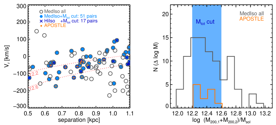
Figure 3: Left: Separation vs. relative radial velocity of halo pair members in DOVE. Open circles indicate MedIso sample galaxies (see text for details). Filled blue circles correspond to a subsample of MedIso pairs that further satisfies a total mass cut of $\log\,((M_{200,1}+M_{200,2})/\rm M_{\odot})=[12.2,12.6]$. Crosses mark HiIso sample galaxies with the aforementioned total mass cut. APOSTLE pairs, which are a subsample of the MedIso sample, are highlighted with small orange circles. Dotted lines indicate timing argument solutions for total masses of $\log(M/\rm M_{\odot})=12.2$ and $12.6$, as labelled. Right: Total mass, i.e. $M_{200,1}+M_{200,2}$, distribution of all the MedIso pairs shown in the left hand panel. The shaded blue region indicates the additional total mass constraint of $\log(M_{\rm tot}/\rm M_{\odot})=[12.2,12.6]$. An orange histogram shows the total mass distribution of APOSTLE pairs.

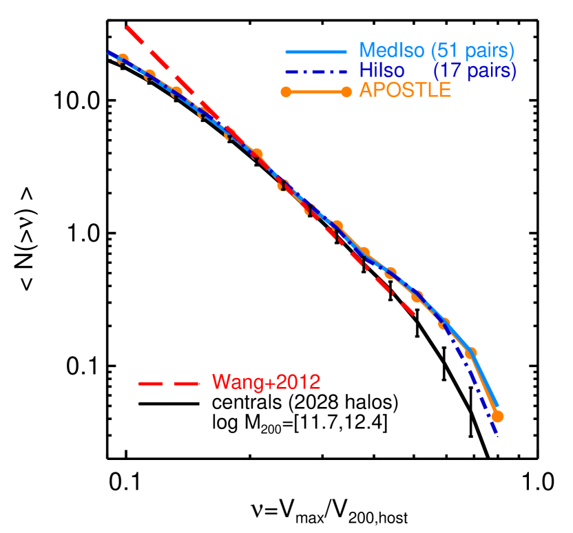
Figure 4: Subhalo $V_{\rm max}$ function, normalized by the host virial velocity $V_{200}$ (i.e. $\nu=V_{\rm max}/V_{200,\rm host}$), for subhaloes within $r_{200}$ of MW-mass haloes in DOVE. The black line corresponds to the average result for 2028 subhaloes around isolated haloes with mass $\log(M_{200}/\rm M_{\odot})=[11.7,12.4]$. The fit to the normalized $V_{\rm max}$ function from Wang et al. (2012) is shown with the red dashed line. The average relation for haloes in the MedIso and HiIso pair samples are presented with the light-blue solid line and dark blue dashed-dotted line, respectively. The average result for subhaloes around APOSTLE primaries is shown with the orange connected circles. Error bars on the black line indicate the $\pm 1\sigma$ dispersion around the mean, calculated from 1000 102-halo samples randomly drawn from the DOVE catalogue (same number as MedIso primaries).

3.1 Frequency of LMC-mass satellites

Fig. 2 shows that, out of 24 APOSTLE primaries, $14$ host nearby satellites massive enough to be comparable to the LMC. Of these, 11 are within the virial radius of their host at $z=0$. This is a relatively high frequency somewhat unexpected compared with earlier findings from large cosmological simulations. Indeed, in the Millenium-II (MS-II) DM-only simulation only $8$ to $27\%$ of MW-mass haloes with virial masses between $1$ and $2.5\times 10^{12}\,M_{\odot}$ are found to host a subhalo at least as massive as that of the LMC within their virial radii (Boylan-Kolchin et al., 2010).

This apparent tension motivates us to consider potential environmental effects that may affect the presence of massive satellites. The Local Group environment, after all, is characterized by a very particular configuration, with a close pair of halos of comparable mass approaching each other for the first time. Could this environment favor the presence and/or late accretion of massive satellites into the primaries, compared with isolated halos of similar mass?

We explore this using the DOVE simulation, where we identify pairs of haloes according to well-defined mass, separation, and isolation criteria in an attempt to approximate the properties of the Local Group environment. We start by selecting haloes with virial masses $M_{200}>5\times 10^{11}\rm M_{\odot}$ and select those that are within (0.5-1.1) Mpc of another halo in the same mass range. We impose then a mass ratio cut of $M_{200,2}/M_{200,1}>0.3$, in order to retain pairs with comparable mass members, and similar to the MW-M31 pair. (Here $M_{200,1}$ refers to the virial mass of the more massive halo of the pair; $M_{200,2}$ to the other.)

We apply next an isolation criterion such that there is no halo (or subhalo) more massive than $M_{200,2}$ within $r_{\rm iso}=2.5$ Mpc, measured from the midpoint of the pair. A stricter isolation criteria is defined by increasing the isolation radius to $r_{\rm iso}=5$ Mpc. Following Fattahi et al. (2016), we refer to the first isolation as “MedIso” and to the stricter one as “HiIso”.

We do not distinguish between centrals and non-centrals in our pair selection. In fact, in some cases, pair members share the same FoF group. These are always the two most massive subhaloes of their FoF group. Our isolation criterion discards pairs of haloes that are satellites of a more massive halo.

The relative radial velocity vs. separation of all MedIso pairs is presented in the left panel of Fig. 3 with open circles. The total mass, $M_{\rm tot}=M_{200,1}+M_{200,2}$, of these pairs span a wide range as shown by the grey histrogram in the right-hand panel of Fig. 3. We further select only pairs with total mass in the range $\log(M_{\rm tot}/\rm M_{\odot})=[12.2,12.6]$, as marked by the blue shaded region in the right panel. This range includes the total masses of all APOSTLE pairs (yellow histogram in the right panel). MedIso pairs that satisfy this total mass criterion are highlighted with blue filled circles in the left panel. This mass cut excludes pairs with the largest total masses and most extreme relative radial velocities, which are outliers from the timing-argument predictions for two point-masses on a radial orbit approaching each other for the first time (red dotted curves labelled by the value of $\log M_{\rm tot}/M_{\odot}$) .

We shall hereafter refer as “MedIso sample” to the final sample of DOVE pairs (with 51 pairs) that satisfy all the above “Local Group criteria”, summarized below:

• separation: $0.5$-$1.1\,{\rm Mpc}$

• minimum mass of individual haloes: $M_{200}>5\times 10^{11}\rm M_{\odot}$

• comparable mass pair members: $M_{200,2}/M_{200,1}>0.3$

• total mass of pairs: $\log(M_{200,1}+M_{200,2})/M_{\odot}=[12.2,12.6]$

• MedIso isolation: $r_{\rm iso}=2.5\,{\rm Mpc}$

The final “HiIso sample”, with 17 pairs, satisfies all the above conditions but has a stricter isolation criterion of $r_{\rm iso}=5\,{\rm Mpc}$. These are marked with crosses in Fig. 3.

APOSTLE pairs are a subsample of the MedIso group, but with extra constraints on the relative radial and tangential velocity between the primaries, as well as on the Hubble flow velocities of objects surrounding the primaries out to 4 Mpc (see Fattahi et al., 2016, for details). They are marked with small orange filled circles in the left panel of Fig. 3, and their total mass distribution is shown by the orange histogram in the right-hand panel of the same figure.

We compare in Fig. 4 the abundance of (massive) subhaloes around APOSTLE primaries with those of MedIso and HiIso pairs, as well as with all isolated MW-mass haloes in DOVE. The latter is a “control sample” that includes all central subhalos with $11.7<\log(M_{200}/M_{\odot})<12.4$ found in the DOVE cosmological box. This mass range covers the range of masses of individual pair members in APOSTLE and in the MedIso sample.

Fig. 4 shows the scaled subhalo $V_{\rm max}$ function, i.e. $N(>\nu)\equiv N(>V_{\rm max}/V_{\rm 200,host})$, averaged over host haloes in various samples. We include all subhaloes within $r_{200}$ of the hosts. The scaled subhalo $V_{\rm max}$ function of the control sample (solid black curve) is consistent with the fit from Wang et al. (2012), who used a number of large cosmological simulations and a wide halo mass range (red dashed curve). The turnover at $\nu<0.15$ is an artifact of numerical resolution, which limits our ability to resolve very low mass haloes.

Interestingly, Fig. 4 shows that, on average, our various paired samples (MedIso, HiIso, APOSTLE) have an overabundance of massive subhaloes relative to average isolated $\sim 10^{12}\,M_{\odot}$ haloes. Indeed, the chance of hosting a massive subhalo with $\nu>0.6$ almost doubles for halos in LG-like environments compared with isolated halos.

Error bars on the $\nu$ function of the control sample represent the $\pm 1\sigma$ dispersion around the average, computed by randomly drawing 102 halos (as the total number of halos in the MedIso paired sample) from the sample of 2028 DOVE centrals, 1000 times. We find that only 2/1000 realizations reach the $\langle N(\nu)\rangle$ measured for APOSTLE pairs at $\nu=0.6$, proving the robustness of the result.

We note that the overabundance of massive subhaloes in halo pairs persists when altering the isolation criterion (HiIso vs. MedIso) or when using a more restrictive selection criteria on the relative kinematics of the halos and the surrounding Hubble flow (APOSTLE vs. MedIso). We have additionally checked that imposing tighter constraints directly on the MedIso sample ($V_{r}=[-250,0]\,\,{\rm km\,s^{-1}}$, $d=[0.6,1]\,\,{\rm Mpc}$) does not alter these conclusions. Moreover, we have explicitly checked that the higher frequency of massive satellites found in the paired halo samples is not enhanced by the most massive primaries in the host mass range considered ($11.7<\log(M_{200}/M_{\odot})<12.4$). Therefore, the main environmental driver for the overabundance of massive subhalos in Local Group-like environments seems to be the presence of the halo pair itself.

This result is consistent with that of Garrison-Kimmel et al. (2014), who report a global overabundance of subhalos in Local Group-like pairs compared to isolated MW-like halos. However, we caution that some of the volumes analysed by these authors were specifically selected to contain LMC-like objects, so it is not straightforward to compare our results quantitatively with theirs. We conclude that haloes in pairs such as those in the Local Group have a genuine overabundance of massive satellites compared to isolated halos. LMC-like satellites are thus not a rare occurrence around Milky Way-like hosts.

3.2 The orbits of LMC analogues

LMC analogues should not only match approximately the LMC’s stellar mass (Fig. 2) but also its orbital properties and dynamical configuration. We therefore refine our identifying criteria by inspecting the orbits of the $14$ LMC-analogue candidates, shown in Fig. 5. We shall retain as LMC analogues only candidates that have been accreted relatively recently (i.e., those that undergo the first pericentric passage at times $t_{\rm fper}>10$ Gyr, or $z_{\rm fper}<0.37$) and that, in addition, have pericentric distances $r_{\rm peri}\lesssim 110$ kpc.

Fig. 5 shows that $9$ out of the $14$ original candidates satisfy these conditions (this final sample of LMC analogues is shown in red in Fig. 2). We highlight the orbits of the selected candidates in Fig. 5 using black curves, where the cyan and red circles indicate their pericentres and apocentres, respectively. The rest of the candidates that do not meet the orbital criteria are shown in grey. Of these, we find only one case with a very early first pericentre (at $t\sim 8.7$ Gyr) that is at present on its second approach. The others have either not yet reached pericentre by $z=0$ or have very large ($\sim 200$ kpc) pericentric distances. The APOSTLE LMC analogues are thus recently accreted satellites, in line with the conclusions of Boylan-Kolchin et al. (2011), who find that $50\%$ of massive satellites in the MS-II DMO simulation have infall times in the last 4 Gyrs.

We list the individual pericentric and apocentric distances of each of our 9 LMC analogues in Table 2. The median pericentre is $\sim 60$ kpc, in good agreement with the pericentre estimates for the LMC at $\sim 50$ kpc. The analogues show a wide range of apocentres, which extend from $\sim 260$ kpc all the way to $700$ kpc, with a median of $\sim 420$ kpc. The typical orbit of LMC analogues in our sample is therefore quite eccentric, with a median eccentricity $\epsilon\equiv r_{\rm peri}/r_{\rm apo}=0.12$.

One may use these typical values to draw inferences regarding the past orbital history of the LMC around the MW. For example, taking the LMC’s current Galactocentric radial distance as pericentre distance (i.e., $r_{\rm peri}^{\rm LMC}=49.9$ kpc; see Table 1) the median eccentricity, $\epsilon=0.12$, suggests an apocentre for the LMC of $r_{\rm apo}^{\rm LMC}\sim 408$ kpc before starting its infall towards our Galaxy.

The large apocentric distances discussed above allow the $9$ LMC analogues to acquire substantial angular momentum through tidal torqing by the nearby mass distribution. Table 2 lists the specific orbital angular momentum of each simulated LMC analogue at first pericentre normalized by the virial value ($r_{200}\times V_{200}$) of the corresponding primaries measured at the same time. The median of the sample is $|\vec{l}_{\rm orb}|/(r_{200}\times V_{200})=0.64$, in good agreement with the value ($\sim 0.54$) estimated assuming the latest LMC kinematics constraints from Table 1 (Kallivayalil et al., 2013) and a virial mass $M_{200}=1\times 10^{12}\;\rm M_{\odot}$ for the MW. Under the condition of recent infall, the large orbital spin of the LMC around the Galaxy is not difficult to reproduce within $\Lambda$CDM (see also Boylan-Kolchin et al., 2011).

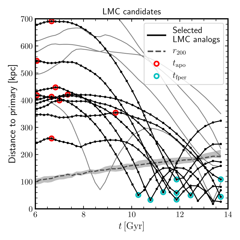
Figure 5: Radial distance to the primary versus time, for the $14$ LMC analogues identified in Fig. 2. The final $9$ LMC analogues analyzed in this work are shown in black, while the rest of candidates are shown in gray. A cyan circle highlights the time when the LMC analogue is at first pericentre. Red circles mark the time of “turnaround” (first apocentre). The average time evolution of the virial radius of the primaries is shown with a dashed line (median and 25-75 percentiles).

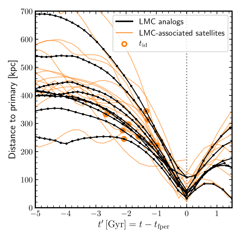
Figure 6: Radial distance to the primary versus time for LMC analogues (black) and LMC-associated satellites (orange). The time axis has been shifted so that all objects are at their first pericentre at $t^{\prime}=0$. The times at which LMC-associated satellites have been identified around their corresponding LMC analogues (’identification time’, $t_{\rm id}$), are highlighted with orange circles.

Table 1: Observational data assumed in this work for the LMC. Stellar mass, Galactocentric position and velocity, Galactocentric radial distance and magnitude of the specific orbital angular momentum vector. Galactocentric Cartesian position has been computed from the RA, dec and $(m-M)$ values quoted in the latest data being made available by the McConnachie (2012) compilation. Galactocentric velocities have been computed assuming a heliocentric line-of-sight velocity of $V_{\rm los}=262.3$ km/s (van der Marel et al., 2002) and proper motions $\mu_{W}=-1.899$ mas/yr, $\mu_{N}=0.416$ mas/yr (Kallivayalil et al., 2013). We assume a distance of the Sun from the Milky Way of $R_{\odot}=8.29$ kpc, a circular velocity of the local standard of rest (LSR) of $V_{0}=239$ km/s (McMillan, 2011), and a peculiar velocity of the Sun with respect to the LSR of $(U_{\odot},V_{\odot},W_{\odot})=(11.1,12.24,7.25)$ km/s (Schönrich et al., 2010).

$M_{*}$/M⊙	$X$/kpc	$Y$/kpc	$Z$/kpc	$V_{X}$/km s-1	$V_{Y}$/km s-1	$V_{Z}$/km s-1	Distance/kpc	$|\vec{l_{\rm orb}}|$/(kpc km s-1)
2.5$\times 10^{9}$	-0.58	-41.77	-27.47	-85.41	-227.49	225.29	49.99	16221.26

Table 2: Orbital characteristics of the $9$ LMC analogues presented in this work. Column 1 indicates the LMC analogue identifier. LMC analogues are identified with a label in the form Vol-FoF-Sub, that indicates the corresponding APOSTLE volume, as well as the FoF and subfind indices of the object in the $z=0$ snapshot. Column 2 indicates the redshift at which the LMC analogue’s corresponding satellites have been identified (‘identification time’ $t_{\rm id}$, see Sec. 4). Throughout this paper, LMC analogues and their respective satellites are shown in a same color consistently in all figures. LMC analogues in this table are ordered by this color, from red to dark blue. Subsequent columns indicate the LMC analogue’s pericentric distance, apocentric distance, orbital eccentricity ($\epsilon=r_{\rm peri}/r_{\rm apo}$), and magnitude of the specific orbital angular momentum vector $\vec{l}_{\rm orb}$ normalized by ($r_{200}\times V_{200}$) of its corresponding primary.

Label	$z_{\rm id}$	$r_{\rm peri}$/kpc	$r_{\rm apo}$/kpc	$\epsilon$	$|\vec{l_{\rm orb}}|$/($r_{200}\times V_{200}$)
5-2-2	0.503	51.00	412.94	0.12	0.72
2-1-3	0.399	32.83	447.37	0.07	0.51
1-1-1	0.366	61.29	544.97	0.11	0.64
12-1-4	0.399	34.14	259.27	0.13	0.33
11-1-4	0.333	58.32	399.28	0.15	0.66
11-1-3	0.302	49.59	418.20	0.12	0.51
10-1-2	0.241	44.25	420.76	0.11	0.28
1-2-2	0.183	108.52	354.17	0.31	0.64
3-1-1	0.302	108.12	690.90	0.16	0.77
Median		50.99	418.19	0.12	0.64

4 LMC-associated satellites in APOSTLE

Given the relatively high masses of the LMC analogues, we expect them to harbour their own population of satellite dwarfs. We identify them in the simulations as follows. We first trace their orbits back from pericentre until they are $\sim 100$ kpc away from the virial boundary of the primary. At that time in the orbit, referred to as “identification time", or $t_{\rm id}$, we flag as “LMC satellites” all luminous subhalos within $100$ kpc of each LMC analogue. We include all luminous subhalos; i.e., with at least 1 star particle, unless otherwise specified.

The procedure yields a combined total of $16$ satellites for the $9$ LMC analogues. Only one LMC analogue is “luminous satellite-free” at $t_{\rm id}$. We have traced the orbital evolution of the LMC satellites in time and have confirmed that all are bound to their LMC analogues, at least until first pericentre. One of the satellites merges with its LMC analogue before the latter reaches first pericentre. Our final sample therefore consists of $15$ LMC-associated satellites.

Using merger trees, we trace back and forth in time each of the LMC-associated satellites. We show their orbits in Fig. 6 with orange curves, together with those of their respective primaries. Times in this figure have been shifted so that $t^{\prime}=t-t_{\rm fper}=0$ corresponds to that of the snapshot corresponding to the closest approach of each LMC analogue. “Identification times" for each LMC analogue are highlighted with orange circles in Fig. 6.

This figure shows that, at first pericentre, LMC-associated satellites remain very close in radial distance to their corresponding LMC analogue, although they may evolve differently afterwards. This implies, as suggested in Sec. 1, that any MW satellite associated with the LMC should be found at a close distance from the LMC today. We shall return to this issue in Sec. 5.

Hereafter, all the results shown correspond to $t_{\rm fper}$, unless otherwise stated.

4.1 Projected position and orbital angular momentum

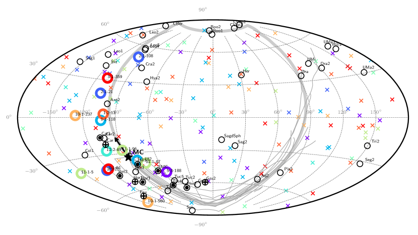
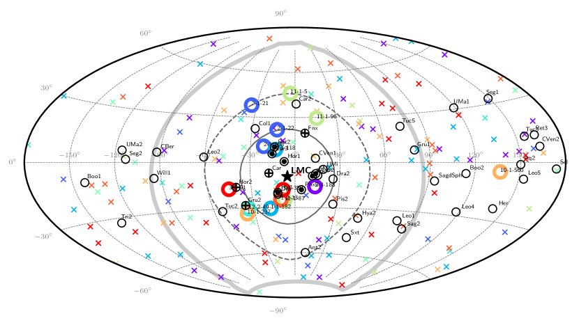
Figure 7: Position (top) and orbital angular momentum direction (bottom) of satellites of the primary haloes relative to the LMC (black star), in Galactocentric coordinates. LMC-associated satellites are shown as large open circles with labels. The rest of satellites of the primary are shown as crosses. Satellites belonging to the same primary are shown in the same color. Coordinates systems are rotated such that the positions and orbital poles of LMC analogues coincide with the corresponding observed values for the LMC, indicated with a large star. Observed MW satellites are shown as open black circles with labels. MW satellites highlighted with a filled circle or a cross are those deemed likely LMC associates according to the discussion in Sec. 5. Thin gray lines in the top panel show the individual orbital trajectories of each of the 9 LMC analogues. An arrow indicates the direction of motion of the LMC along the trajectory. In the bottom panels, for reference, we show circles centred on the LMC with aperture $32^{\circ}$ and $55^{\circ}$, respectively (see text for details).

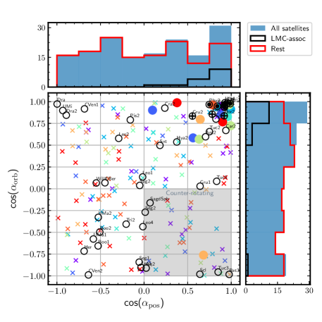
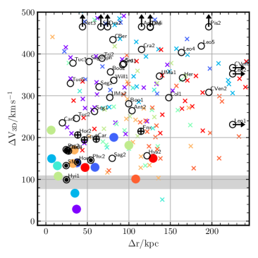
Figure 8: Left: Angular separation between the position vector of satellites and that of the LMC analogue, versus angular separation between the orbital angular momentum direction of satellites and that of the LMC analogue. LMC-associated satellites from APOSTLE are shown as colored filled circles, and the rest of satellites as crosses. Histograms show the distribution along the axes of the different samples of satellites (i.e., all satellites, LMC-associated satellites, and the rest of satellites of the primary). Right: Radial distance and 3D velocity of LMC-associated satellites relative to that of their LMC analogue, at first pericentre. A shaded band indicates the 25-75 percentile range of $V_{\rm max}$ values for LMC analogues, as a reference. Color-coding in both panels is the same as in Fig. 7. For comparison, MW satellites are shown as black open circles with labels. MW satellites highlighted with a filled circle or a cross are those deemed likely LMC associates according to the discussion in Sec. 5.

The top panel of Figure 7 shows an Aitoff projection of the sky position of all satellites associated with the primaries hosting LMC analogues at the time of first pericentre. Each of the coordinate systems of the 9 LMC analogues has been rotated so that the LMC analogue is at the same Galactocentric position in the sky as the observed LMC and the orbital angular momentum vector of the LMC analogue is parallel to that of the observed LMC (see Table 1 for the position and velocity data assumed for the LMC). The position of the LMC (analogue and observed) is marked with a star, while LMC-associated satellites are shown as large colored open circles with labels. The remainder of the satellites of each primary are shown as colored crosses. A different color is used for each of the 9 primaries containing LMC analogues.

For comparison, observed MW satellites are overplotted as small black open circles with identifying labels. In addition, a thick gray line marks the LMC’s orbital plane and an arrow indicates the direction of motion along this line. Individual thin gray lines show each of the LMC analogues’ orbital paths, starting at “turnaround” (apocentre) and ending at pericentre. One interesting result is that APOSTLE LMC analogues mostly follow the same orbital plane during their infall onto the primary. This is in good agreement with Patel et al. (2017b), who find LMC-mass satellites in the Illustris simulations with late accretion times generally conserve their orbital angular momentum up to $z=0$.

The spatial distribution in the sky of the LMC-associated satellites clearly delineates the orbital plane of the LMC, which appear to spread more or less evenly along the leading and trailing section of the orbital path, as expected if LMC satellites were to accompany the orbit of the LMC. The bottom panel of Figure 7 shows that this is indeed the case: the instantaneous direction of the orbital angular momentum vectors (or orbital ’poles’) of LMC-asociated satellites at $t_{\rm fper}$ seems to coincide rather well with that of the LMC itself. Again the coordinate system of each LMC analogue has been rotated such that the LMC analogue’s orbital pole aligns with that of the observed LMC, marked with a star.

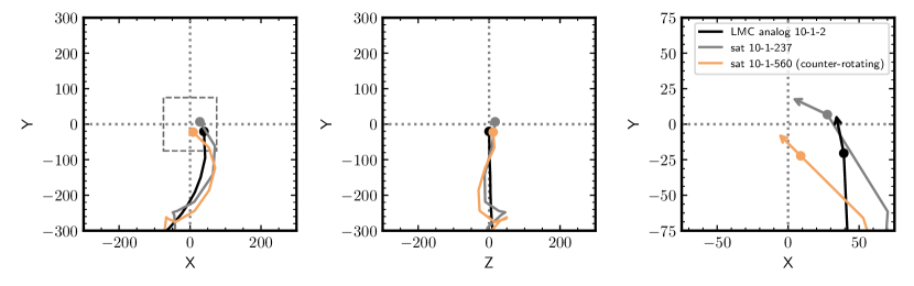
Figure 9: Orbital trajectory of the LMC-associated satellite (labelled 10-1-560, see Fig. 7) that appears to be counter-orbiting with respect to its LMC analogue at the time of first pericentre (in orange). The trajectory of the LMC analogue is shown in black. A second satellite of the same LMC analogue is shown in grey. The reference system is centred on the primary galaxy, and the orbital plane of the LMC analogue is chosen as the XY plane. The rightmost panel is a zoomed-in view of the region enclosed in a rectangle in the leftmost panel. Arrows in the right-most panel indicate the direction of the instantaneous velocity vectors of each satellite at the final time.

The clustering of the orbital poles of LMC-associated satellites is to be expected although it is perhaps less tight than assumed in earlier work (see Fig.5 of Kallivayalil et al., 2018). Indeed, some satellites are found to have orbital poles that differ from that of the LMC by as much as $\sim 55$ degrees (shown as a dashed-line circle for reference), with a median value of $\sim 32$ degrees (shown as a solid-line circle).

The spatial and pole distributions on the sky of LMC-associated satellites in APOSTLE are consistent with the location of the bulk of the debris from the cosmological dark matter-only LMC analogue studied first in Sales et al. (2011); Sales et al. (2017) and compared to Gaia data in Kallivayalil et al. (2018). However, we find also a surprising result here: there is the case of a simulated satellite whose orbital pole is nearly 180 degrees away from its LMC analogue’s. In other words, this satellite appears to be “counter-rotating” the Milky Way relative to the LMC (see orange open circle labelled 10-1-560 in Fig. 7). We shall explore this case in more detail in Sec. 4.2.

One conclusion from Fig. 7 is that the orbital pole condition leaves many MW satellites as potentially associated with the LMC. It is therefore important to look for corroborating evidence using additional information, such as positions and velocities. We explore this in Fig. 8, where the left panel shows the cosine of the angle between different directions that relate the LMC with its satellites. The x-axis corresponds to the angular distance ($\alpha_{\rm pos}$) between the position of the LMC analogue and other satellites; the y-axis indicates the angular distance ($\alpha_{\rm orb}$) between their corresponding orbital poles.

Satellites associated with LMC analogues are shown with colored circles in Fig. 8, and are compared with those of MW satellites with available data (open black circles). The former are clearly quite close to the LMC both on the sky in position (most have $\cos\alpha_{\rm pos}>0.5$), and also have closely aligned orbital poles (most have $\cos\alpha_{\rm orb}>0.5$).

What about the other satellites, which were not associated with the LMC analogues before infall? Are their positions and/or kinematics affected by the LMC analogue? Apparently not, as shown by the small colored crosses in Fig. 8 and by the histograms at the top and right of the left-hand panel of the same figure. Filled blue histograms show the distribution of each quantity (for simulated satellites) on each axis. These show a small enhancement towards small values of $\alpha_{\rm pos}$ and $\alpha_{\rm orb}$, but the enhancement is entirely due to the satellites associated with the LMC analogues (black histograms). Subtracting them from the total leaves the red histogram, which is consistent with a flat, uniform distribution. In other words, neither the angular positions nor the orbital angular momentum directions of non-associated satellites seems to be noticeably affected by a recently accreted LMC analogue.

Besides the projected distance and orbital pole separation shown on the left panel of Fig. 8, our results also indicate that satellites associated with the LMC analogues remain close in relative distance and velocity (something already hinted at when discussing Fig. 6). This is shown in the right-hand panel of Fig. 8, where we plot the relative velocity ($\Delta V_{\rm 3D}$) and distance ($\Delta r$) between all satellites of the primary and the LMC analogue. Satellites associated with the analogues (filled circles) clearly cluster towards small $\Delta r$ and small $\Delta V_{\rm 3D}$, with a median $\Delta r$ of just $\sim 37$ kpc and a median $\Delta V_{\rm 3D}$ of just $\sim 138$ km/s. We shall use these results to refine our criteria for identifying LMC-associated satellites in Sec. 5, after considering first the peculiar case of a counter-rotating satellite.

4.2 A counter-rotating LMC-associated satellite

We turn our attention now to the “counter-rotating” satellite highlighted in the Aitoff projection in Fig. 7 (orange open circle labelled 10-1-560), which appears at $\cos(\alpha_{\rm orb})\sim-0.75$ in the left panel of Fig. 8. This is clearly an outlier relative to all other satellites associated with LMC analogues. What mechanism could explain this odd orbital motion?

With hindsight the explanation is relatively simple, and may be traced to a case where the amplitude of the motion of a satellite around the LMC analogue is comparable to the pericentric distance of the latter around the primary host. This is shown in Fig. 9, which plots the orbital trajectory of satellite 10-1-560 in a reference frame centred on the primary and where the XY plane is defined to coincide with the orbital plane of the LMC analogue. The LMC analogue is shown in black, and its two satellites in grey and orange. In all panels, a line shows the trajectory of each object starting at early times and finalizing at first pericentre (marked with a circle), which, in this particular case, corresponds with the last snapshot of the simulation, at $z=0$. The left and middle panels show the XY and ZY projections of the trajectories in a box $600$ kpc on a side. The right-hand panel shows a zoomed-in XY view $150$ kpc on a side, where the arrows indicate the projections of the instantaneous velocity vectors at first pericentre.

The velocity vectors explain clearly why satellite 10-1-560 appears to counter-rotate: when the relative “size” of the LMC satellite system is comparable to the pericentric distance of the LMC orbit, the orbital motion may appear to carry an LMC satellite on an instantaneous orbit that shares the same orbital plane but that goes around the primary centre on the opposite side. We find this instance in only one out of the $15$ satellites we identified and tracked. This is thus a possible but relatively rare occurrence which should, however, be kept in mind when considering the likelihood of association of satellites that may pass all other criteria but are found to have orbital planes approximately counter-parallel to the LMC.

4.3 Contribution of LMC analogues to the primary satellite population

We consider now the contribution of satellites of LMC analogues to the satellite population of the primary galaxy. The cyan curve in Fig. 10 shows the average satellite mass function of all $24$ APOSTLE primaries at $z=0$, and compares it to that of the $9$ primaries with LMC analogues (at the time of their first pericentric passage; orange curve). Specifically, we consider all satellites within the virial radius of the primary ($\sim 200$ kpc on average). The grey curve shows the MW satellite population for reference (see Table 3). All MW satellites in our study are found within $\sim 250$ kpc of the MW centre, a distance that compares well with the virial radii of APOSTLE primaries.

The overall good agreement of APOSTLE with the MW satellite population is reassuring, as it suggests that the simulated populations are realistic and that their mass functions may be used to shed light on the impact of the LMC on the overall MW satellite population. Comparing the orange and cyan curves indicates that LMC analogues have, as expected, a substantial impact on the massive end of the satellite population, but, aside from that, the effect on the whole population of satellites with $M_{*}>10^{5}\,M_{\odot}$ is relatively modest. Indeed, the $9$ primaries with LMC analogues have $17.8^{+8.0}_{-1.2}$ (median and 25-75 percentiles) such satellites, compared with the average $16.1^{+6.3}_{-3.8}$ for all $24$ primaries and with $16.3^{+4.6}_{-3.2}$ for the $15$ APOSTLE primaries without LMC analogues. In other words, aside from the presence of the LMC itself, the impact of the LMC satellites on the overall satellite population is relatively minor.

This is also shown by the green curve in Fig. 10, which indicates the (average) satellite mass function of the LMC analogues at identification time, $t_{\rm id}$ (i.e., before infall). The $9$ LMC analogues contribute a total of $16$ dwarfs with $M_{*}>10^{5}\,M_{\odot}$ at infall, or roughly $\sim 10\%$ of the satellite population of each primary. In terms of numbers, the average $\langle\rm N_{\rm sat}(M_{*}>10^{5}M_{\odot})\rangle$ is $16/9=1.8\pm 0.9$, where the error range specifies the $\pm 1\sigma$ spread of the distribution. The green circles at the bottom of Fig. 10 show the individual stellar masses of each satellite in our $9$ LMC analogues. None of our LMC analogues has a companion as massive as the SMC, which has a stellar mass of order $M_{*}\sim 3\times 10^{8}\,M_{\odot}$. Most satellites contributed by LMC analogues have stellar masses $M_{*}<10^{6}\,M_{\odot}$.

We note that the relatively modest impact of the LMC on the MW massive satellite population suggested by our results is consistent with the early semi-analytical models of Dooley et al. (2017), as well as with other studies of isolated LMC-mass systems using the FIRE simulations (Jahn et al., 2019) and simulations from the Auriga project (Pardy et al., 2020).

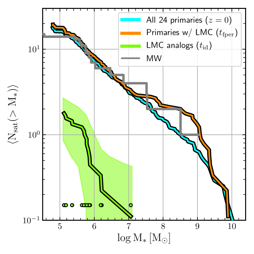
Figure 10: Average satellite mass function for all the 24 primaries in AP-L2 runs at $z=0$ (cyan). This agrees fairly well with the observed satellite mass function in the MW (gray line). The satellite mass function of the $9$ primaries that contain a LMC analogue is shown in orange for comparison, and suggests an excess on the high-mass end due largely to the LMC analogue itself. On average, LMC analogues contribute roughly 10% of all satellites with $M_{*}>10^{5}\;\rm M_{\odot}$ to their primaries (green curve). The shaded area shows the $\pm 1\sigma$ dispersion range. Green symbols show the individual masses of satellites identified in our $9$ LMC analogues.

4.4 LMC and the radial distribution of satellites

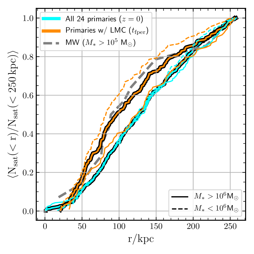
Figure 11: Average cumulative radial distribution of satellites within 250 kpc, for (i) all the 24 primaries in APOSTLE-L2, at $z=0$ (cyan); (ii) the primaries of the 9 LMC analogues, at first pericentre (orange); and (iii) the Milky Way satellites. We include in all of these samples only satellites with $M_{*}>10^{5}\,M_{\odot}$. Thinner lines show the distributions for simulated satellites filtered by stellar mass as quoted in the legend. Note that the MW satellite distribution appears more concentrated than the average APOSTLE primary; this is well matched by systems with an LMC analogue, a transient configuration that results from the particular orbital configuration of the LMC and its satellites (at pericentre).

The radial distribution of satellites contains important clues to the accretion history of a galaxy (see; e.g., Samuel et al., 2020; Carlsten et al., 2020, and references therein). Recent results from the SAGA survey have suggested that "the radial distribution of MW satellites is much more concentrated than the average distribution of SAGA satellites, mostly due to the presence of the LMC and SMC" (Mao et al., 2020). We explore below whether our simulations confirm that this effect is likely due to the LMC and its satellites.

The cyan curve in Fig. 11 shows the average cumulative radial distribution of all $M_{*}>10^{5}\,M_{\odot}$ satellites within $250$ kpc of the $24$ APOSTLE primaries. The corresponding MW satellite population is significantly more concentrated, as shown by the grey dashed curve in the same figure. Interestingly, the $9$ APOSTLE primaries with LMC analogues, shown by the orange curve, also have more concentrated satellite distributions, in good agreement with the MW satellite population.

This is mainly a transient result of the particular orbital phase of the LMC analogues, which are chosen to be near first pericentric passage. Indeed, at $z=0$ the same $9$ primaries have less centrally concentrated distributions, consistent with the average result for all $24$ primaries (cyan curve). Support for our interpretation of the transient concentration as due to the LMC analogues and their associated satellite systems is provided by the thin orange lines in Fig. 11. The dashed and solid (thin) orange lines indicate results for systems with stellar mass exceeding or smaller than $10^{6}\,M_{\odot}$. The higher concentration is only apparent in the latter case: this is consistent with our earlier finding that LMC analogues contribute mainly systems with $M_{*}<10^{6}\,M_{\odot}$ (see Fig. 10).

We conclude that the concentrated radial distribution of satellites in the Galaxy is probably a transient caused by the presence of the LMC and its satellites near first pericentre. This transient effect illustrates the importance of taking into account the particular kinematic stage of the LMC when comparing the properties of the Galactic satellite population with that of other external galaxies.

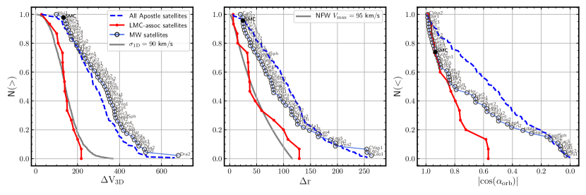
Figure 12: Cumulative distributions of the three diagnostics used to rank MW satellites in terms of likely association with the LMC. These diagnostics are the 3D velocity relative to the LMC ($\Delta V_{\rm 3D}$, left), the radial distance relative to the LMC ($\Delta r$, centre) and the alignment with the LMC’s orbital pole direction ($|\rm cos(\alpha_{\rm orb})|$, right). A red line shows the cumulative distribution for LMC-associated satellites in APOSTLE; a dashed blue line shows that for all APOSTLE satellites, and a black line shows the distribution for all MW satellites, as labelled. For reference, the grey curve in the $\Delta V_{\rm 3D}$ panel (left) shows a Gaussian distribution with $\sigma_{\rm 1D}=90$ km/s. In the $\Delta r$ panel (centre) the grey curve shows the cumulative mass profile of an NFW dark matter halo with $V_{\rm max}=95$ km/s, roughly the average $V_{\rm max}$ of the APOSTLE LMC analogues.

5 LMC-associated satellites in the Milky Way

We have seen in the above subsections that satellites associated with LMC-analogues contribute modestly to the primary satellite population, and distinguish themselves from the rest of a primary’s satellites by their proximity in phase space to their parent LMC analogue. Satellites closely aligned in orbital pole direction, and at small relative distances and velocities from the LMC, should be strongly favoured in any attempt to identify which MW satellites have been contributed by the LMC.

We may compile a ranked list of potential associations by assigning to all MW satellites numerical scores on each of the above diagnostics. This score consists of a numerical value equal to the fraction of associated satellites in the simulations that are farther from their own LMC analogue in each particular dignostic (i.e., a score of $1$ means that a particular satellite is closer to the LMC than all simulated satellites, in that diagnostic.). We illustrate this scoring procedure in Fig. 12.

The left panel shows the cumulative distribution of $\Delta V_{\rm 3D}$, the relative velocity between the LMC and other satellites. The red curve corresponds to all simulated satellites associated to LMC analogues, the dashed blue curve to all satellites of APOSTLE primaries. The grey curve shows the cumulative distribution expected if associated satellites had a Gaussian isotropic velocity distribution around the analogue with a velocity dispersion of $\sigma_{\rm 1D}=90$ km/s. For example, the SMC (highlighted in Fig. 12 with a filled circle) has $\Delta V_{\rm 3D}=133$ km/s, which gives it a relatively high score of $\sim 0.59$ in this diagnostic. According to this diagnostic, any MW satellite whose LMC relative velocity exceeds $\sim 220$ km/s has a score of zero, and its association with the LMC is in doubt.

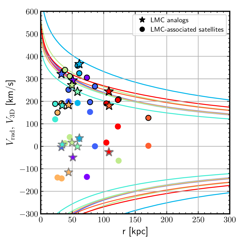
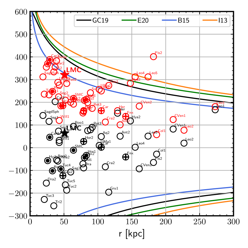
Figure 13: Radial velocity $V_{\rm rad}$ and 3D velocity $V_{\rm 3D}$ versus radial distance, at pericentre. Left: APOSTLE LMC analogues (stars) and LMC-associated satellites (circles). Radial (3D) velocities are shown with symbols with grey (black) edges. Lines illustrate the escape velocity profiles of the corresponding primaries. Color-coding is the same as in previous figures. Right: observed MW satellites at $z=0$. Radial velocities are shown in black, and 3D velocities in red. The LMC is marked with a star. Observed $V_{\rm rad}$ and $V_{\rm 3D}$ are from Fritz et al. (2018) when available, or computed from measured kinematic data as explained in Tab. 3. Lines show the escape velocity profiles derived from the following MW models proposed in the literature: Garavito-Camargo et al. (2019); Errani & Peñarrubia (2020); Bovy (2015); Irrgang et al. (2013).

The middle and right panels of Fig. 12 show the other two diagnostics we have chosen to rank possible LMC-associated satellites. The middle panel indicates the relative distance between satellites and the LMC. The red curve again corresponds to simulated satellites associated with LMC analogues. Its distribution is very well approximated by the radial mass profile of an NFW halo with $V_{\rm max}=90$ km/s and concentration $c=10.2$ (grey curve). For reference, the median $V_{\rm max}$ and 10-90 percentiles for LMC analogues is $78^{+52}_{-16}$ km/s (see Fig. 2). Together with the evidence from the left panel, this confirms that satellites associated with LMC analogues are, at first pericentre, distributed around the analogues more or less as they were before infall. Tides, again, have not yet had time to disrupt the close physical association of the Magellanic group in phase space. The SMC, for example, scores $\sim 0.76$ in this diagnostic.

Finally, the right-hand panel of Fig. 12 shows the orbital pole alignment, where we have chosen to use the absolute value of $\cos(\alpha_{\rm orb})$ in order to account for the possibility of “counter-rotating” satellites. The SMC, again, scores high in this diagnostic; with a score of $\sim 0.72$ for $|\cos(\alpha_{\rm orb})|=0.93$. In this case, any MW satellites with $|\cos(\alpha_{\rm orb})|<0.57$ would have a score of zero.

We may add up the three scores to rank all MW satellites according to the likelihood of their association of the LMC. The data and scores are listed in Table 3, and show that, out of $46$ MW satellites, $11$ have non-zero scores in all three categories. Of these $11$, the $7$ whose association appears firm are: Hydrus 1, SMC, Car 3, Hor 1, Tuc 4, Ret 2, and Phx 2. These $7$ satellites are highlighted with a solid central circle in the figures throughout the paper. A second group with more tenuous association, mainly because of their large relative velocity difference, contains Carina, Hor 2, and Grus 2. The final member is Fornax, whose scores in relative velocity and position are non-zero but quite marginal. These $4$ satellites are highlighted with a cross in the figures.

Three satellites in this list have $M_{*}>10^{5}\,M_{\odot}$ (SMC, Carina, Fornax). This is actually in excellent agreement with the discussion in Sec. 4.3, where we showed that LMC analogues bring $\sim 2$ such satellites into their primaries. The same arguments suggest that $\sim 10\%$ of all MW satellites might have been associated with the LMC. This small fraction is in tension with the $11$ out of $46$ satellites (i.e., $24\%$) in our list. We note, however, that our current list of MW satellites is likely very incomplete (see; e.g., Newton et al., 2018; Nadler et al., 2020), and highly biased to include more than its fair share of LMC satellites. Indeed, many of the new satellite detections have been made possible by DES, a survey of the southern sky in the vicinity of the Magellanic Clouds (Bechtol et al., 2015; Koposov et al., 2015; Drlica-Wagner et al., 2015).

Our list adds some candidates compared to the lists compiled by earlier work, but also contain some differences. Sales et al. (2011) and Sales et al. (2017) identified only three satellites as clearly associated with the LMC: the SMC, Hor 1 and Tuc 2. The latter is, however, deemed unlikely given our analysis, especially because of its large LMC relative velocity, $\Delta V_{\rm 3D}=246$ km/s. Kallivayalil et al. (2018)’s list of possible LMC-associated satellites includes Car 2, Draco 2, and Hydra 2. According to our analysis, the first two are ruled out by their large relative velocity. The last one is, on the other hand, ruled out by its large orbital pole deviation.

Erkal & Belokurov (2020) claim SMC, Hydrus 1, Car 3, Hor 1, Car 2, Phx 2 and Ret 2 as associated with the LMC. Using a similar methodology, Patel et al. (2020) also identifies the first 5 as LMC “long term companions”. Of these, our analysis disfavours Car 2, again on account of its large relative velocity, $\Delta V_{\rm 3D}=235$ km/s. Finally, Pardy et al. (2020) argues for Carina and Fornax as candidates for LMC association. Our analysis does not rule out either (both have non-zero scores in all three categories), although the evidence for association is not particularly strong, especially for Fornax. Our results agree with Erkal & Belokurov (2020) in this regard, who argues the need for an uncommonly massive LMC to accomodate Fornax as one of its satellites.

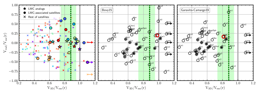
Figure 14: Radial velocity versus total 3D velocity, both normalized by the escape velocity at the pericentric radius. Left: APOSTLE LMC analogues, LMC-associated satellites, and rest of satellites of the corresponding primary at first pericentre. Color-coding is the same as in previous figures. Centre: Observed MW satellites assuming the Bovy (2015) MW potential. Right: Observed MW satellites assuming the Garavito-Camargo et al. (2019) MW potential. A green vertical line with shade shows the median $V_{\rm 3D}/V_{\rm esc}(r)$ and 25-75% percentiles for LMC analogues, and is marked in all panels. In the centre and right panels the observed LMC’s position, as defined by the assumed MW escape velocity, is highlighted with a red open circle. Objects with $V_{\rm 3D}/V_{\rm esc}(r)>1$ are gravitationally unbound to the primary given that choice of potential.

6 The LMC and the escape velocity of the Milky Way

We have argued in the preceding sections that, because the LMC is just past its first pericentric passage, then its associated satellites must still be close in position and velocity. Other corollaries are that both the LMC and its satellites must have Galactocentric radial velocities much smaller than their tangential velocities, and that their total velocities must approach the escape velocity of the Milky Way at their location.

We explore this in the left panel of Fig. 13, which shows the radial ($V_{\rm rad}$) and total 3D velocities ($V_{\rm 3D}$) of LMC analogues (stars) and LMC-associated satellites (circles) at the LMC analogue’s first pericentre, as a function of their radial distance to the primary. Radial velocities are shown as symbols without edges, and 3D velocities as symbols with dark edges. A different color is used for each of the 9 LMC-analogue systems.

All LMC-analogues and most of their associated satellites are close to pericentre and have therefore radial velocities much smaller than their total velocities: half of the LMC analogues have $|V_{\rm rad}|/V_{\rm 3D}<0.10$, and half of the $15$ associated satellites have $|V_{\rm rad}|/V_{\rm 3D}<0.43$. (For reference, the LMC itself has $|V_{\rm rad}|/V_{\rm 3D}\approx 0.2$.)

It is also clear from the left panel of Fig. 13 that the large majority of LMC analogues have total velocities that trace closely the escape velocity of each of their primaries at their location. This is interesting because many commonly used models for the MW potential are calibrated to match observations in and around the solar circle, but differ in the outer regions of the Galaxy, near the location of the LMC.

This is illustrated in the right-hand panel of Fig. 13, where the 4 different curves show the escape velocity curves corresponding to models recently proposed for the Milky Way; i.e., those of Irrgang et al. (2013, I13), Bovy (2015, B15), Garavito-Camargo et al. (2019, GC19), and Errani & Peñarrubia (2020, E20). These models differ in their predicted escape velocities at the location of the LMC ($r\sim 50$ kpc) from a low value of $\sim 330$ km/s (B15) to a high value of $\sim 445$ km/s (I13). The LMC could therefore provide useful additional information about the total virial mass of the MW, which dominates any estimate of the escape velocity.

We explore this in more detail in the left panel of Fig. 14, where we show the radial and total velocity of LMC analogues and their satellites, expressed in units of the escape velocity at their current location. The median $V_{\rm 3D}/V_{\rm esc}$ and 25-75% percentiles for LMC analogues is $0.88^{+0.07}_{-0.15}$, a value that we indicate with a shaded green line. For LMC-associated satellites the corresponding value is similar; $0.82^{+0.11}_{-0.15}$, again highlighting the close dynamical correspondence between LMC analogues and their satellites. The high velocity of LMC-associated systems differs systematically from that of regular satellites (i.e., those not associated with LMC analogues, shown with colored crosses in Fig. 14). These systems have $V_{\rm 3D}/V_{\rm esc}=0.59^{+0.18}_{-0.14}$.

The well-defined value of $V_{\rm 3D}/V_{\rm esc}$ for LMC analogues allows us to estimate the MW escape velocity at $50$ kpc from the total Galactocentric velocity of the LMC, estimated at $V_{\rm 3D}\approx 320$ km/s by Kallivayalil et al. (2013). This implies $V_{\rm esc}^{\rm MW}$(50 kpc)$\approx 365$ km/s, favouring models with modest virial masses for the MW. The four models shown in the right-hand panel of Fig. 13 have $V_{\rm esc}(50\,\rm kpc)=$ 397 (GC19); 413 (E20); 330 (B15); 445 (I13) km/s. Of these, the closest to our estimate is that of GC19, which has a virial mass of $M_{200}=1.2\times 10^{12}\,M_{\odot}$. Interestingly, this is also the mass favored by the recent analysis of stellar halo kinematics by Deason et al. (2020).

Further constraints may be inferred by considering simulated satellites with velocities higher than the local escape speed. These are actually quite rare in our APOSTLE simulations: only $2$ LMC-associated satellites and $3$ regular satellites (out of a total of $163$) appear “unbound”. We compare this with observed MW satellites in Fig. 14, where the middle panel corresponds to the B15 model potential and the right-hand panel to that of GC19. (MW satellite Galactocentric radial and 3D velocities are taken from Fritz et al. (2018) if available, or otherwise computed from measured kinematic data as explained in the caption to Tab. 3.) Although the LMC $V_{\rm 3D}/V_{\rm esc}$ seems acceptable in both cases, assuming the B15 potential would yield $8$ escaping satellites out of $46$, a much higher fraction than expected from the simulations. Even after removing Hya 2, Leo 4, Leo 5 and Pis 2, which are distant satellites with large velocity uncertainties (in all these cases exceeding $\sim 250$ km/s), the fraction of escapers would still be $\sim 10\%$, much larger than predicted by APOSTLE.

The GC19 potential fares better, with three fewer escapers than B15: Gru 1, Car 3 and Boo 2 are all comfortably bound in this potential. Hya 2, Leo 4, Leo 5 and Pis 2 are still unbound, however. Indeed, Leo 5 and Pis 2 would be unbound even in the I13 potential, the most massive of the four, with a virial mass $M_{200}=1.9\times 10^{12}\,M_{\odot}$. Should the velocities/distances of those satellites hold, it is very difficult to see how to reconcile their kinematics with our simulations, unless those velocities are substantially overestimated. Tighter, more accurate estimates of their kinematics should yield powerful constraints on the Galactic potential.

7 Summary and Conclusions

We have used the APOSTLE suite of cosmological hydrodynamical simulations to study the accretion of LMC-mass satellites into the halo of MW-sized galaxies. APOSTLE consists of simulations of $12$ cosmological volumes selected to resemble the Local Group. Each volume includes a pair of halos with halo masses, separation, and relative radial and tangential velocities comparable to the MW and M31. We identify “LMC analogues” as massive satellites of any of the 24 APOSTLE primary galaxies. These satellites are chosen to be representative of the recent accretion of the LMC into the Galactic halo, taking into account the LMC stellar mass and its particular kinematic state near the first pericentric passage of its orbit.

Our results allow us to address the role of the LMC (the most massive Galactic satellite) on the properties of the MW satellite population, including (i) the frequency of LMC-mass satellites around MW-sized galaxies and the effects of the Local Group environment; (ii) observational diagnostics of possible association between MW satellites and the LMC before infall, (iii) the contribution of the LMC to the population of “classical” satellites of the MW; and (iv) the constraints on the MW gravitational potential provided by the LMC motion. To our knowledge, this is the first study of “LMC analogues” and their satellite companions carried out in realistic Local Group cosmological hydrodynamical simulations.

Our main results may be summarized as follows.

• We find that $14$ out of $24$ primaries in APOSTLE have a satellite of comparable mass to the LMC ($8.75\leq\log M_{*}/M_{\odot}\leq 10$) within 350 kpc at $z=0$. This is a higher fraction than estimated in previous work. We use the DOVE simulation to study the frequency of massive satellites around MW-mass haloes that are isolated and in pairs. The high frequency of LMC analogues in APOSTLE seems to have an environmental origin, as LMC-like companions are roughly twice more frequent around primaries in Local Group-like environments than around isolated halos of similar mass.

• Out of the $14$ LMC analogues, we select a subsample of $9$ which have reached their first pericentric passage in the past $4$ Gyr. These satellites inhabit $M_{200}\sim 10^{11}$ M_⊙ halos before infall, and have rather eccentric orbits, with median pericentric and apocentric distances of $\sim 60$ kpc and $\sim 420$ kpc, respectively.

• LMC analogues host their own satellites and contribute them to the primary satellite population upon infall. We find a total of $16$ LMC-associated satellites before infall with $M_{*}>10^{5}\;\rm M_{\odot}$ for the $9$ LMC analogues, or slightly fewer than $2$ “classical” satellites per LMC. One satellite merges with the LMC analogue before first pericentre. The LMC satellites contribute, on average, about $\sim 10\%$ of the total population of primary satellites.

• In agreement with previous work, we find that at the time of first pericentre, LMC-associated satellites are all distributed close to, and along, the orbital plane of the LMC, extending over $\sim 45^{\circ}$ along the leading and trailing part of the orbit. Their orbital angular momentum vectors are aligned with that of the LMC, with a median relative angle of $32^{\circ}$.

• We report one case of an LMC-associated satellite that is apparently counter-rotating the primary compared with the LMC. The apparent counter-rotation may result when the orbital motion of the satellite around the LMC is comparable or larger than the pericentric distance of the LMC. Under some circumstances, this leads the satellite to approach the centre of the primary “on the other side” relative to the LMC. This is relatively rare, and only one of the $15$ LMC-associated satellites appears to “counter-rotate”.

• We find that LMC-associated satellites are located very close to their LMC analogue in position and velocity, with a median relative radial distance of $\sim 37$ kpc and a median relative 3D velocitys of $\sim 138$ km/s. This is because there has not been enough time for tidal interactions from the MW to disperse the original orbits of LMC-companion satellites.

• We may use the proximity of associated satellites to the LMC in phase space to rank MW satellites according to the likelihood of their LMC association. We find that $11$ out of $46$ MW satellites could in principle be LMC associates. For $7$ of those the association appears firm: Hydrus 1, SMC, Car 3, Hor 1, Tuc 4, Ret 2, and Phx 2. Others, such as Carina, Hor 2, Grus 2 and Fornax are potential associates as well, but their large LMC relative velocities weakens their case.

• The radial distribution of the satellite populations of primaries with LMC analogues is more concentrated than those of average APOSTLE primaries. This effect is largely driven by the particular kinematic stage of the LMC, near its first pericentric passage, and largely disappears after the LMC (and its associated satellites) move away from pericentre. This offers a natural explanation for the more concentrated radial distribution of satellites in the MW compared to observed MW-analogues in the field, as recently reported by the SAGA survey (Mao et al., 2020).

• The 3D velocity of LMC analogues near first pericentre is very close to the escape velocity of their primaries, with a median $V_{\rm 3D}/V_{\rm esc}\approx 0.9$. We may use this result to derive an estimate for the MW’s escape velocity at the location of the LMC ($r\sim 50$ kpc) of $\sim 365$ km/s. We also find that very few simulated satellites (fewer than roughly $1$ in $30$) are unbound from their primaries. This information may be used to discriminate between different models of the MW potential. We find the model proposed by Garavito-Camargo et al. (2019) to be in reasonable agreement with our constraints, suggesting a MW virial mass of roughly $1\times 10^{12}\,M_{\odot}$.

Our analysis shows that $\Lambda$CDM simulations of the Local Group can easily account for the properties of the Magellanic accretion into the halo of the Milky Way, and offer simple diagnostics to guide the interpretation of extant kinematic data when attempting to disentangle Magellanic satellites from the satellite population of the Milky Way. The accretion of the LMC and its associated satellites into the Milky Way seems fully consistent with the hierarchical buildup of the Galaxy expected in the $\Lambda$CDM paradigm of structure formation.

Table 3: Values and ’scores’ of MW satellites according to the different diagnostics used in this paper to assess association with the LMC: the 3D velocity relative to the LMC ($\Delta V_{\rm 3D}$), the radial distance relative to the LMC ($\Delta r$), and the alignment with the LMC’s orbital pole direction ($|\rm cos(\alpha_{\rm orb})|$). MW satellites are ordered according to their total score in these 3 categories (last column). The 11 MW satellites which we consider in this paper may be possibly associated to the LMC according to APOSTLE predictions (i.e., those with non-zero scores in all 3 categories) are highlighted in red. Column 3 indicates if the satellite is co-rotating (+) or counter-rotating (-) the primary with respect to the LMC. Column 4 shows the stellar mass of MW satellites, computed applying a mass-to-light ratio to the $V$-band luminosities in McConnachie (2012)’s database. We assume $M_{*}/L_{V}=1.6$ for all satellites (appropriate for dSph-type galaxies) except for the SMC, where $M_{*}/L_{V}=0.7$ has been used (see Woo et al., 2008). We consider all MW satellites for which kinematic data is available. For all satellites we adopt the positions and distance moduli data (RA, dec, $(m-M)$) in McConnachie (2012)’s database. Line-of-sight velocities and proper motions have been taken from Fritz et al. (2018) (their Table 2) when available, and otherwise from McConnachie & Venn (2020) (Tables 1 and  4). SMC kinematic data is from Kallivayalil et al. (2013). Galactocentric positions and velocities have been computed assuming a distance of the Sun from the Milky Way of $R_{\odot}=8.29$ kpc, a circular velocity of the local standard of rest (LSR) of $V_{0}=239$ km/s (McMillan, 2011), and a peculiar velocity of the Sun with respect to the LSR of $(U_{\odot},V_{\odot},W_{\odot})=(11.1,12.24,7.25)$ km/s (Schönrich et al., 2010).

MW satellite		Sign	$M_{*}$/($10^{5}$M⊙)	$\Delta V_{\rm 3D}$/km s-1	$\Delta r$/kpc	$\rm|cos(\alpha_{\rm orb})|$	Score $\Delta V_{\rm 3D}$	Score $\Delta r$	Score $|\rm cos(\alpha_{\rm orb})|$	Total Score
Hydrus1	Hyi1	+	0.10	99.01	24.87	0.98	0.87	0.76	0.97	2.60
SMC	SMC	+	3229.22	132.97	24.47	0.93	0.59	0.76	0.72	2.07
Horologium1	Hor1	+	0.04	141.33	38.19	0.99	0.45	0.46	1.00	1.91
Carina3	Car3	+	0.01	168.75	25.81	0.96	0.27	0.76	0.86	1.89
Tucana4	Tuc4	+	0.03	167.70	27.29	0.95	0.28	0.75	0.82	1.84
Reticulum2	Ret2	+	0.05	171.09	24.43	0.94	0.26	0.76	0.73	1.76
Phoenix2	Phx2	+	0.03	145.83	54.18	0.97	0.42	0.36	0.95	1.73
Tucana3	Tuc3	-	0.01	378.12	32.64	0.96	0.00	0.73	0.84	1.57
Carina	Car	+	8.09	196.22	60.69	0.98	0.15	0.33	0.99	1.47
Reticulum3	Ret3	-	0.03	487.03	44.15	0.98	0.00	0.42	0.99	1.41
Sculptor	Scl	-	29.12	525.06	66.25	0.98	0.00	0.31	0.98	1.30
Horologium2	Hor2	+	0.01	206.19	38.43	0.84	0.11	0.46	0.50	1.07
Grus2	Gru2	+	0.05	194.33	46.43	0.83	0.15	0.41	0.49	1.05
Draco	Dra	+	4.17	463.86	125.79	0.97	0.00	0.08	0.96	1.04
CanesVenatici2	CVen2	-	0.16	308.17	196.32	0.99	0.00	0.00	1.00	1.00
Carina2	Car2	+	0.09	235.30	19.87	0.67	0.00	0.78	0.17	0.96
Segue1	Seg1	-	0.00	262.35	58.59	0.84	0.00	0.34	0.51	0.85
Draco2	Dra2	+	0.02	679.81	74.32	0.84	0.00	0.29	0.52	0.81
Crater2	Cra2	+	2.61	410.77	115.22	0.93	0.00	0.11	0.70	0.81
Aquarius2	Aq2	-	0.08	518.58	115.28	0.91	0.00	0.11	0.66	0.77
Tucana5	Tuc5	+	0.01	329.49	29.56	0.09	0.00	0.74	0.00	0.74
Fornax	Fnx	+	331.22	215.01	114.53	0.86	0.08	0.11	0.54	0.73
Tucana2	Tuc2	+	0.05	245.89	36.80	0.66	0.00	0.54	0.17	0.71
CanesVenatici1	CVen1	+	3.73	367.17	254.35	0.92	0.00	0.00	0.68	0.68
UrsaMinor	UMi	+	5.60	470.43	125.73	0.90	0.00	0.08	0.60	0.67
Leo5	Leo5	-	0.08	419.04	187.19	0.90	0.00	0.00	0.61	0.61
Sagittarius2	Sag2	+	0.17	150.34	79.92	0.04	0.33	0.27	0.00	0.61
Columba1	Col1	+	0.09	295.47	148.11	0.80	0.00	0.00	0.41	0.41
Hydra2	Hya2	+	0.09	156.49	121.81	0.54	0.31	0.09	0.00	0.40
Pisces2	Pis2	+	0.07	492.15	196.14	0.79	0.00	0.00	0.39	0.39
SagittariusdSph	SagdSph	-	343.65	381.88	52.08	0.16	0.00	0.37	0.00	0.37
Bootes1	Boo1	-	0.35	280.81	99.81	0.66	0.00	0.20	0.17	0.37
Segue2	Seg2	-	0.01	321.30	64.08	0.27	0.00	0.32	0.00	0.32
Antlia2	Ant2	+	5.60	264.32	103.77	0.60	0.00	0.17	0.14	0.31
Triangulum2	Tri2	-	0.01	389.81	67.73	0.41	0.00	0.31	0.00	0.31
UrsaMajor2	UMa2	-	0.07	296.04	76.99	0.33	0.00	0.28	0.00	0.28
Bootes2	Boo2	-	0.02	357.00	77.87	0.50	0.00	0.28	0.00	0.28
ComaBerenices	CBer	+	0.08	434.12	80.77	0.07	0.00	0.27	0.00	0.27
Willman1	Will1	+	0.01	336.92	81.77	0.07	0.00	0.27	0.00	0.27
Grus1	Gru1	+	0.03	374.43	92.55	0.03	0.00	0.23	0.00	0.23
Sextans	Sxt	+	6.98	376.57	93.79	0.50	0.00	0.22	0.00	0.22
Hercules	Her	-	0.29	342.98	164.59	0.72	0.00	0.00	0.20	0.20
Leo2	Leo2	+	10.77	352.40	255.00	0.58	0.00	0.00	0.11	0.11
UrsaMajor1	UMa1	-	0.15	347.02	136.85	0.58	0.00	0.00	0.10	0.10
Leo1	Leo1	+	70.49	231.14	262.99	0.14	0.00	0.00	0.00	0.00
Leo4	Leo4	-	0.14	403.60	163.35	0.43	0.00	0.00	0.00	0.00

Data availability

The simulation data underlying this article can be shared on reasonable request to the corresponding author. The observational data for Milky Way satellites used in this article comes from the following references: Kallivayalil et al. (2013, see http://www.astro.uvic.ca/~alan/Nearby_Dwarf_Database_files/NearbyGalaxies.dat, and references therein); Fritz et al. (2018, see http://www.astro.uvic.ca/~alan/Nearby_Dwarf_Database_files/NearbyGalaxies.dat, and references therein); McConnachie & Venn (2020, see http://www.astro.uvic.ca/~alan/Nearby_Dwarf_Database_files/NearbyGalaxies.dat, and references therein); McConnachie (2012, see http://www.astro.uvic.ca/~alan/Nearby_Dwarf_Database_files/NearbyGalaxies.dat, and references therein).

References

- Bechtol et al. (2015) Bechtol K., et al., 2015, ApJ, 807, 50
- Behroozi et al. (2013) Behroozi P. S., Wechsler R. H., Conroy C., 2013, ApJ, 770, 57
- Besla et al. (2007) Besla G., Kallivayalil N., Hernquist L., Robertson B., Cox T. J., van der Marel R. P., Alcock C., 2007, ApJ, 668, 949
- Bovy (2015) Bovy J., 2015, ApJS, 216, 29
- Boylan-Kolchin et al. (2010) Boylan-Kolchin M., Springel V., White S. D. M., Jenkins A., 2010, MNRAS, 406, 896
- Boylan-Kolchin et al. (2011) Boylan-Kolchin M., Besla G., Hernquist L., 2011, MNRAS, 414, 1560
- Busha et al. (2011) Busha M. T., Marshall P. J., Wechsler R. H., Klypin A., Primack J., 2011, ApJ, 743, 40
- Campbell et al. (2017) Campbell D. J. R., et al., 2017, MNRAS, 469, 2335
- Carlsten et al. (2020) Carlsten S. G., Greene J. E., Peter A. H. G., Greco J. P., Beaton R. L., 2020, ApJ, 902, 124
- Crain et al. (2015) Crain R. A., et al., 2015, MNRAS, 450, 1937
- D’Onghia & Fox (2016) D’Onghia E., Fox A. J., 2016, ARA&A, 54, 363
- D’Onghia & Lake (2008) D’Onghia E., Lake G., 2008, ApJ, 686, L61
- Davis et al. (1985) Davis M., Efstathiou G., Frenk C. S., White S. D. M., 1985, ApJ, 292, 371
- Deason et al. (2020) Deason A. J., et al., 2020, arXiv e-prints, p. arXiv:2010.13801
- Dooley et al. (2017) Dooley G. A., Peter A. H. G., Carlin J. L., Frebel A., Bechtol K., Willman B., 2017, MNRAS, 472, 1060
- Drlica-Wagner et al. (2015) Drlica-Wagner A., et al., 2015, ApJ, 813, 109
- Erkal & Belokurov (2020) Erkal D., Belokurov V. A., 2020, MNRAS, 495, 2554
- Errani & Peñarrubia (2020) Errani R., Peñarrubia J., 2020, MNRAS, 491, 4591
- Fattahi et al. (2016) Fattahi A., et al., 2016, MNRAS, 457, 844
- Fattahi et al. (2018) Fattahi A., Navarro J. F., Frenk C. S., Oman K. A., Sawala T., Schaller M., 2018, MNRAS, 476, 3816
- Fritz et al. (2018) Fritz T. K., Battaglia G., Pawlowski M. S., Kallivayalil N., van der Marel R., Sohn S. T., Brook C., Besla G., 2018, A&A, 619, A103
- Gaia Collaboration et al. (2018) Gaia Collaboration et al., 2018, A&A, 616, A12
- Garavito-Camargo et al. (2019) Garavito-Camargo N., Besla G., Laporte C. F. P., Johnston K. V., Gómez F. A., Watkins L. L., 2019, ApJ, 884, 51
- Garrison-Kimmel et al. (2014) Garrison-Kimmel S., Boylan-Kolchin M., Bullock J. S., Lee K., 2014, MNRAS, 438, 2578
- Irrgang et al. (2013) Irrgang A., Wilcox B., Tucker E., Schiefelbein L., 2013, A&A, 549, A137
- Jahn et al. (2019) Jahn E. D., Sales L. V., Wetzel A., Boylan-Kolchin M., Chan T. K., El-Badry K., Lazar A., Bullock J. S., 2019, MNRAS, 489, 5348
- Jenkins (2013) Jenkins A., 2013, MNRAS, 434, 2094
- Jethwa et al. (2016) Jethwa P., Erkal D., Belokurov V., 2016, MNRAS, 461, 2212
- Kallivayalil et al. (2013) Kallivayalil N., van der Marel R. P., Besla G., Anderson J., Alcock C., 2013, ApJ, 764, 161
- Kallivayalil et al. (2018) Kallivayalil N., et al., 2018, ApJ, 867, 19
- Kim et al. (1998) Kim S., Staveley-Smith L., Dopita M. A., Freeman K. C., Sault R. J., Kesteven M. J., McConnell D., 1998, ApJ, 503, 674
- Komatsu et al. (2011) Komatsu E., et al., 2011, ApJS, 192, 18
- Koposov et al. (2015) Koposov S. E., Belokurov V., Torrealba G., Evans N. W., 2015, ApJ, 805, 130
- Mao et al. (2020) Mao Y.-Y., Geha M., Wechsler R. H., Weiner B., Tollerud E. J., Nadler E. O., Kallivayalil N., 2020, arXiv e-prints, p. arXiv:2008.12783
- McConnachie (2012) McConnachie A. W., 2012, AJ, 144, 4
- McConnachie & Venn (2020) McConnachie A. W., Venn K. A., 2020, AJ, 160, 124
- McMillan (2011) McMillan P. J., 2011, MNRAS, 414, 2446
- Moster et al. (2013) Moster B. P., Naab T., White S. D. M., 2013, MNRAS, 428, 3121
- Nadler et al. (2019) Nadler E. O., Mao Y.-Y., Green G. M., Wechsler R. H., 2019, ApJ, 873, 34
- Nadler et al. (2020) Nadler E. O., et al., 2020, ApJ, 893, 48
- Newton et al. (2018) Newton O., Cautun M., Jenkins A., Frenk C. S., Helly J. C., 2018, MNRAS, 479, 2853
- Pardy et al. (2020) Pardy S. A., et al., 2020, MNRAS, 492, 1543
- Patel et al. (2017a) Patel E., Besla G., Sohn S. T., 2017a, MNRAS, 464, 3825
- Patel et al. (2017b) Patel E., Besla G., Mandel K., 2017b, MNRAS, 468, 3428
- Patel et al. (2020) Patel E., et al., 2020, ApJ, 893, 121
- Qu et al. (2017) Qu Y., et al., 2017, MNRAS, 464, 1659
- Sales et al. (2007) Sales L. V., Navarro J. F., Abadi M. G., Steinmetz M., 2007, MNRAS, 379, 1475
- Sales et al. (2011) Sales L. V., Navarro J. F., Cooper A. P., White S. D. M., Frenk C. S., Helmi A., 2011, MNRAS, 418, 648
- Sales et al. (2013) Sales L. V., Wang W., White S. D. M., Navarro J. F., 2013, MNRAS, 428, 573
- Sales et al. (2017) Sales L. V., et al., 2017, MNRAS, 464, 2419
- Samuel et al. (2020) Samuel J., et al., 2020, MNRAS, 491, 1471
- Sawala et al. (2016) Sawala T., et al., 2016, MNRAS, 457, 1931
- Schaye et al. (2015) Schaye J., et al., 2015, MNRAS, 446, 521
- Schönrich et al. (2010) Schönrich R., Binney J., Dehnen W., 2010, MNRAS, 403, 1829
- Shao et al. (2018) Shao S., Cautun M., Deason A. J., Frenk C. S., Theuns T., 2018, MNRAS, 479, 284
- Springel (2005) Springel V., 2005, MNRAS, 364, 1105
- Springel et al. (2001) Springel V., Yoshida N., White S. D. M., 2001, New A, 6, 79
- Tollerud et al. (2011) Tollerud E. J., Boylan-Kolchin M., Barton E. J., Bullock J. S., Trinh C. Q., 2011, ApJ, 738, 102
- Wang et al. (2012) Wang J., Frenk C. S., Navarro J. F., Gao L., Sawala T., 2012, MNRAS, 424, 2715
- Westerlund (1990) Westerlund B. E., 1990, A&A Rev., 2, 29
- Woo et al. (2008) Woo J., Courteau S., Dekel A., 2008, MNRAS, 390, 1453
- Yozin & Bekki (2015) Yozin C., Bekki K., 2015, MNRAS, 453, 2302
- van der Marel & Kallivayalil (2014) van der Marel R. P., Kallivayalil N., 2014, ApJ, 781, 121
- van der Marel et al. (2002) van der Marel R. P., Alves D. R., Hardy E., Suntzeff N. B., 2002, AJ, 124, 2639