Detecting Sparse Heterogeneous Mixtures in a Two-Sample Problem

Abstract

We consider the problem of detecting sparse heterogeneous mixtures in a two-sample setting from a nonparametric perspective, where the effect manifests itself as a positive shift. We suggest a two-sample higher criticism test, and show that it is first-order comparable to the likelihood ratio test for the generalized Gaussian mixture models in all sparsity regimes.

1 Introduction

The detection of sparse mixtures has been studied for decades [9, 7]. Most work has focused on detecting deviation of data from the known distribution. However, in practice, it’s more common that we do not have access to the null distribution and have to estimate it from a control group. For example, in a clinical trial, patients were assigned to two groups randomly, given either the placebo or the treatment. For some reasons, the treatment could only affect a small proportion of the patients treated, while the remaining patients reacted the same as patients in the control group. Similar settings were investigated in Conover and Salsburg [6] and they modeled the shift in the distribution as a Lehmann alternative and focused on the locally most powerful tests.

We study this situation in parallel with the work of Ingster [9] and Donoho and Jin [7]. Let $F$ and $G$ be two continuous (unknown) distribution functions on the real line. We consider the following hypothesis testing problem: based on a random sample $X_{1},\cdots,X_{m}$ drawn iid from $F$ and another independent random sample $Y_{1},\cdots,Y_{n}$ drawn iid from $G$, decide

$$\mathcal{H}_{0}:G=F\quad\text{versus}\quad\mathcal{H}_{1}:G=(1-\varepsilon)F+\varepsilon F(\cdot-\mu),\quad\varepsilon>0,\quad\mu>0.$$ (1)

where $\varepsilon\in(0,1/2)$ is the fraction of non-null effect and $\mu$ is the size of the location shift. Hence, under the alternative, $G$ is stochastic larger than $F$. We assume that

$$\lim_{m,n\to\infty}\frac{n}{m+n}=\eta\in(0,1/2]$$ (2)

at a sufficient fast rate.

The optimum of rank tests was mainly investigated as locally most powerful [12]. Following the line of our work in the one-sample setting, we still focus on the asymptotically optimum here. As usual, a testing procedure is asymptotically powerful (resp. powerless) if the sum of its probabilities of Type I and Type II errors (its risk) has limit 0 (resp. inferior at least 1) in the large sample asymptote.

1.1 A benchmark: generalized Gaussian mixture model

The normal mixture model has been studied in Ingster [9] considering the one-sample setting, that is, $F$ is known to be standard normal and only the $Y$-sample is collected. The problem is investigated in various asymptotic regimes defined by how fast $\varepsilon$ goes to zero. The detection boundary of the likelihood ratio test (LRT) (then any other tests) is derived. Donoho and Jin [7] further derived the detection boundary when $F$ is generalized Gaussian:

$$f(x)\propto\exp\Big{(}-\frac{|x|^{\gamma}}{\gamma}\Big{)},$$ (3)

where $\gamma>0$. Note that $\gamma=2$ corresponds to the normal distribution and $\gamma=1$ corresponds to the double-exponential distribution. They parameterized $\varepsilon=\varepsilon_{n}$ as

$$\varepsilon_{n}=n^{-\beta},\quad 0<\beta<1\text{ fixed}.$$ (4)

In the sparse setting where $1/2<\beta<1$, let

$$\mu_{n}=(\gamma r\log n)^{1/\gamma},\quad 0<r<1\text{ fixed},$$ (5)

then the detection boundary when $\gamma>1$ is

$$\rho^{*}_{\gamma}(\beta)=\begin{cases}(2^{1/(\gamma-1)}-1)^{\gamma-1}(\beta-\frac{1}{2}),&\frac{1}{2}<\beta<1-2^{-\gamma/(\gamma-1)};\\ (1-(1-\beta)^{1/\gamma})^{\gamma},&1-2^{-\gamma/(\gamma-1)}<\beta<1.\end{cases}$$ (6)

and for the case $\gamma\leq 1$

$$\rho^{*}_{\gamma}(\beta)=2\beta-1.$$ (7)

That means, if $r>\rho^{*}(\beta)$, $\mathcal{H}_{0}$ and $\mathcal{H}_{1}$ separate asymptotically, while if $r<\rho^{*}(\beta)$, $\mathcal{H}_{0}$ and $\mathcal{H}_{1}$ merge asymptotically.

The detection boundary in the dense regime where $0<\beta<1/2$ is given in [2]. Let

$$\mu_{n}=n^{s-1/2},\quad 0<s<1/2\text{ fixed},$$ (8)

then the hypotheses merge asymptotically when $s<\beta$ if $\gamma\geq 1/2$ and $s<\frac{1}{2}-\frac{1-2\beta}{1+2\gamma}$ if $\gamma<1/2$.

1.2 The two-sample higher criticism test

The one-sample higher criticism test was suggested in Donoho and Jin [7] and proved to be first-order asymptotically comparable to the LRT in the normal mixture model. In the two-sample setting, an analogous higher criticism statistic was proposed as [5, 8]:

$${\rm HC}=\sup_{t\in\mathbb{R}}\sqrt{\frac{mn}{m+n}}\frac{[F_{m}(t)-G_{n}(t)]}{\sqrt{H_{m+n}(t)(1-H_{m+n}(t))}},$$ (9)

where $F_{m}$ and $G_{n}$ are empirical distributions of the $X$-sample and the $Y$-sample, respectively, and $H_{m+n}(t)=\frac{1}{m+n}(mF_{m}(t)+nG_{n}(t))$ is the empirical distribution of the combined sample. The test rejects for large values of (9). This is to the two-sample Kolmogorov - Smirnov test [15] what the Anderson-Darling test (aka the higher criticism test) is to the Kolmogorov-Smirnov test.

Pettitt [14] proposed the integral version of the two-sample Anderson-Darling statistic and gave an approximation of the distribution. Finner and Gontscharuk [8] studied the supremum version (9) in terms of local levels and focused on the Type I error. It is also connected to the work of Zhao et al [17], which normalizes the Hoeffding test for independence in an analogous way. Note that all these tests are based on ranks only, so they are nonparametric tests. Distribution-free tests for sparse heterogeneous mixtures in the one-sample setting was investigated in [2] where they assumed that $F$ is symmetric about zero and the true effects have positive median. In our work, we do not pose any assumptions on $F$ except it is continuous, and we use the $X$-sample to estimate $F$. In addition, the two-sample higher criticism is parallel to the CUSUM sign test in [2] as the Wilcoxon test to the Wilcoxon signed-rank test [16].

2 Lower bound

The formulation (1) indicates that both the null and the alternative hypotheses are composite. If we assume model parameters $(F,\varepsilon,\mu)$ are known, then the likelihood ratio test (LRT) is the most powerful test by Neyman-Pearson lemma. In particular, if $F$ is given, we don’t need the $X$-sample, then the question is reduced to the one-sample situation [9, 7, 4]. The general detection boundary was given in [3, Lemma A.1] as follows in our context: let $f$ denote the density of $F$, then the hypotheses (1) merge asymptotically when there is a sequence $(x_{n})$ such that

$$n\bar{F}(x_{n})\to 0,\quad n\varepsilon_{n}\bar{F}(x_{n}-\mu_{n})\to 0,$$ (10)

and

$$n\varepsilon^{2}_{n}\Big{[}\int_{-\infty}^{x_{n}}\frac{f(x-\mu_{n})^{2}}{f(x)}dx-1\Big{]}_{+}\to 0.$$ (11)

3 The two-sample higher criticism test

For a distribution $F$, $\bar{F}(x)=1-F(x)$ will denote its survival function.

Theorem 1.

For the testing problem (1) and under (2), the two-sample higher criticism test is asymptotically powerful if either there is a sequence $(t_{n})$ such that $t_{n}\to\infty$,

$$n(\bar{F}(t_{n})\vee\varepsilon\bar{F}(t_{n}-\mu))\gg\log^{2}n,$$ (12)

and

$$\frac{\sqrt{n}\varepsilon[\bar{F}(t_{n}-\mu)-\bar{F}(t_{n})]}{\sqrt{\bar{F}(t_{n})+\varepsilon\eta\bar{F}(t_{n}-\mu)}}\gg\log n;$$ (13)

or $t$ is the median of $F$ and

$$\sqrt{n}\varepsilon[\bar{F}(t-\mu)-\frac{1}{2}]\gg\log n.$$ (14)

Proof.

Finner and Gontscharuk [8] showed that the two-sample HC statistic (9) is almost surely equal to

$${\rm HC}^{*}=\sup_{s\in I_{m,n}}\sqrt{\frac{m+n}{m+n-1}}\frac{[V_{m,s}-\operatorname{\mathbb{E}}_{0}[V_{m,s}]]}{\sqrt{\operatorname{Var}_{0}[V_{m,s}]}},$$ (15)

where $V_{m,s}$ denotes the number of ranks related to the $X$-sample being not larger than $s$ and $I_{m,n}:=\{1,\cdots,m+n-1\}$. They also showed that ${\rm HC}^{*}$ coincides asymptotically in distribution with the one-sample HC statistic with sample size $n$ under the null as we assume that $n\leq m$, which was derived in [10]. Thus, we have

$$\operatorname{\mathbb{P}}_{0}\big{(}{\rm HC}\geq\sqrt{3\log\log n}\big{)}\to 0.$$ (16)

For simplicity, we consider the test with rejection region $\{{\rm HC}\geq\log n\}$. Hence, the test is asymptotically powerful if, under the alternative, there is $t_{n}$ (or $t$) $\in\mathbb{R}$ such that

$$\operatorname{\mathbb{P}}_{1}\Big{(}\sqrt{\frac{mn}{m+n}}\frac{[F_{m}(t_{n})-G_{n}(t_{n})]}{\sqrt{H_{m+n}(t_{n})(1-H_{m+n}(t_{n}))}}\geq\log n\Big{)}\to 1.$$ (17)

Indeed, $mF_{m}(t)$ is binomial with parameters $m$ and $F(t)$, $nG_{n}(t)$ is binomial with parameters $n$ and $G(t)=(1-\varepsilon)F(t)+\varepsilon F(t-\mu)$, and

$$H_{m+n}(t)=\frac{m}{m+n}F_{m}(t)+\frac{n}{m+n}G_{n}(t).$$ (18)

We also define $H(\cdot)$ as

$$H(t)=(1-\eta)F(t)+\eta G(t)=(1-\varepsilon\eta)F(t)+\varepsilon\eta F(t-\mu).$$ (19)

Hence, by Chebyshev’s inequality, we have

$$\frac{\sqrt{m}|F_{m}(t_{n})-F(t_{n})|}{\sqrt{F(t_{n})(1-F(t_{n}))}}\leq\log m$$ (20)

with probability tending to 1, and

$$\frac{\sqrt{n}|G_{n}(t_{n})-G(t_{n})|}{\sqrt{G(t_{n})(1-G(t_{n}))}}\leq\log n$$ (21)

with probability tending to 1. By triangular inequality, we have

$$|F(t_{n})-G(t_{n})| =|F(t_{n})-F_{m}(t_{n})+F_{m}(t_{n})-G_{n}(t_{n})+G_{n}(t_{n})-G(t_{n})|$$ (22)

$$\leq|F(t_{n})-F_{m}(t_{n})|+|F_{m}(t_{n})-G_{n}(t_{n})|+|G_{n}(t_{n})-G(t_{n})|$$ (23)

$$\leq|F_{m}(t_{n})-G_{n}(t_{n})|+\log m\sqrt{\frac{F(t_{n})(1-F(t_{n}))}{m}}+\log n\sqrt{\frac{G(t_{n})(1-G(t_{n}))}{n}}$$ (24)

Hence, we have

$$\sqrt{\frac{mn}{m+n}}\frac{[F_{m}(t_{n})-G_{n}(t_{n})]}{\sqrt{H_{m+n}(t_{n})(1-H_{m+n}(t_{n}))}}\geq a_{n}-b_{n},$$ (25)

where

$$a_{n} :=\sqrt{\frac{mn}{m+n}}\frac{\varepsilon[\bar{F}(t_{n}-\mu)-\bar{F}(t_{n})]}{\sqrt{H_{m+n}(t_{n})(1-H_{m+n}(t_{n}))}},$$ (26)

$$b_{n} :=\sqrt{\frac{n}{m+n}}\log m\sqrt{\frac{F(t_{n})(1-F(t_{n}))}{H_{m+n}(t_{n})(1-H_{m+n}(t_{n}))}}+\sqrt{\frac{m}{m+n}}\log n\sqrt{\frac{G(t_{n})(1-G(t_{n}))}{H_{m+n}(t_{n})(1-H_{m+n}(t_{n}))}},$$ (27)

as we know that $F>G$ under the alternative, and it suffices to show that

$$a_{n}\geq b_{n}+\log n$$ (28)

with probability tending to 1.

$$|\bar{H}_{m+n}(t_{n})-\bar{H}(t_{n})| =\big{|}\frac{m}{m+n}\bar{F}_{m}(t_{n})+\frac{n}{m+n}\bar{G}_{n}(t_{n})-(1-\eta)\bar{F}(t_{n})-\eta\bar{G}(t_{n})\big{|}$$ (29)

$$=\big{|}\frac{m}{m+n}(\bar{F}_{m}(t_{n})-\bar{F}(t_{n}))+(\frac{m}{m+n}-(1-\eta))\bar{F}(t_{n})$$

$$\quad+\frac{n}{m+n}(\bar{G}_{n}(t_{n})-\bar{G}(t_{n}))+(\frac{n}{m+n}-\eta)\bar{G}(t_{n})\big{|}$$ (30)

$$\leq\big{|}\frac{m}{m+n}(\bar{F}_{m}(t_{n})-\bar{F}(t_{n}))|+|\frac{n}{m+n}(\bar{G}_{n}(t_{n})-\bar{G}(t_{n}))\big{|}$$

$$\quad+O\Big{(}\frac{\log n}{\sqrt{n}}\Big{)}(\bar{F}(t_{n})+\bar{G}(t_{n}))$$ (31)

$$\leq\frac{m}{m+n}\log m\sqrt{\frac{\bar{F}(t_{n})(1-\bar{F}(t_{n}))}{m}}+\frac{n}{m+n}\log n\sqrt{\frac{\bar{G}(t_{n})(1-\bar{G}(t_{n}))}{n}}$$

$$\quad+O\Big{(}\frac{\log n}{\sqrt{n}}\Big{)}(\bar{F}(t_{n})+\bar{G}(t_{n}))$$ (32)

$$\asymp O\Big{(}\frac{\log m}{\sqrt{m}}\sqrt{\bar{F}(t_{n})}\Big{)}+O\Big{(}\frac{\log n}{\sqrt{n}}\sqrt{\bar{G}(t_{n})}\Big{)}+O\Big{(}\frac{\log n}{\sqrt{n}}(\bar{F}(t_{n})+\bar{G}(t_{n}))\Big{)}$$ (33)

$$\asymp O\Big{(}\frac{\log n}{\sqrt{n}}\sqrt{(1-\varepsilon)\bar{F}(t_{n})+\varepsilon\bar{F}(t_{n}-\mu)}\Big{)},$$ (34)

as we assume that

$$|\frac{n}{m+n}-\eta|=O(\log n/\sqrt{n}).$$ (35)

Thus, under (12) or (14), we have

$$|\bar{H}_{m+n}(t_{n})-\bar{H}(t_{n})|\ll\bar{H}(t_{n}).$$ (36)

Then if $t_{n}\to\infty$, we have $H(t_{n})\to 1$, and

$$a_{n} =\sqrt{\frac{mn}{m+n}}\frac{\varepsilon[\bar{F}(t_{n}-\mu)-\bar{F}(t_{n})]}{\sqrt{H_{m+n}(t_{n})(1-H_{m+n}(t_{n}))}}$$ (37)

$$\asymp\frac{\sqrt{n(1-\eta)}\varepsilon[\bar{F}(t_{n}-\mu)-\bar{F}(t_{n})]}{\sqrt{(1-\varepsilon\eta)\bar{F}(t_{n})+\varepsilon\eta\bar{F}(t_{n}-\mu)}}\cdot\sqrt{\frac{\bar{H}(t_{n})}{\bar{H}_{m+n}(t_{n})}}$$ (38)

$$\asymp\frac{\sqrt{n}\varepsilon[\bar{F}(t_{n}-\mu)-\bar{F}(t_{n})]}{\sqrt{\bar{F}(t_{n})+\varepsilon\eta\bar{F}(t_{n}-\mu)}}\gg\log n,$$ (39)

under (13).

If $t$ is the median of $F$ such that $F(t)=1/2$, then $H(t)$ is bounded away from 0 and 1, and under condition (14),

$$a_{n} =\sqrt{\frac{mn}{m+n}}\frac{\varepsilon[\bar{F}(t-\mu)-\bar{F}(t)]}{\sqrt{H_{m+n}(t)(1-H_{m+n}(t))}}$$ (40)

$$=\sqrt{n}\varepsilon[\bar{F}(t-\mu)-\frac{1}{2}]\gg\log n.$$ (41)

In addition, we have

$$b_{n}\asymp\log n.$$ (42)

Therefore, (28) is fulfilled eventually. ∎

In the generalized Gaussian mixture model, with parameterization (4) and (5), we choose $t_{n}=(\gamma q\log n)^{1/\gamma}$, $r<q\leq 1$ fixed. By the tail behavior of $F$, we have

$$\bar{F}(t_{n})=L_{n}n^{-q},\quad\bar{F}(t_{n}-\mu_{n})=L_{n}n^{-(q^{1/\gamma}-r^{1/\gamma})^{\gamma}},$$ (43)

where $L_{n}$ denotes any factor logarithmic in $n$.

If $\gamma>1$, we define $r_{\gamma}=(1-2^{-1/(\gamma-1)})^{\gamma}$. If $r<r_{\gamma}$, we set $q=r/r_{\gamma}$. Then the LHS in (12) is

$$n(L_{n}n^{-r/r_{\gamma}}\vee\varepsilon L_{n}n^{-r(r_{\gamma}^{-1/\gamma}-1)^{\gamma}})\asymp L_{n}(n^{1-r/r_{\gamma}}\vee n^{1-\beta-r(r_{\gamma}^{-1/\gamma}-1)^{\gamma}})\gg\log^{2}n.$$ (44)

The LHS in (13) is

$$L_{n}\frac{n^{\frac{1}{2}-\beta}(n^{-r(r_{\gamma}^{-1/\gamma}-1)^{\gamma}}-n^{-r/r_{\gamma}})}{\sqrt{n^{-r/r_{\gamma}}+\varepsilon\eta n^{-r(r_{\gamma}^{-1/\gamma}-1)^{\gamma}}}}\asymp L_{n}(n^{\frac{1+r/r_{\gamma}}{2}-\beta-r(r_{\gamma}^{-1/\gamma}-1)^{\gamma}}\wedge n^{\frac{1}{2}(1-\beta-r(r_{\gamma}^{-1/\gamma}-1)^{\gamma})}),$$ (45)

where both exponents are positive when $r>(2^{1/(\gamma-1)}-1)^{\gamma-1}(\beta-\frac{1}{2})$.

If $r\geq r_{\gamma}$, we set $q=1$. Then the LHS in (12) is

$$n(L_{n}n^{-1}\vee\varepsilon L_{n}n^{-(1-r^{1/\gamma})^{\gamma}})\asymp L_{n}(1\vee n^{1-\beta-(1-r^{1/\gamma})^{\gamma}})\gg\log^{2}n,$$ (46)

if $1-\beta-(1-r^{1/\gamma})^{\gamma}>0$. And the LHS in (13) is

$$L_{n}\frac{n^{\frac{1}{2}-\beta}(n^{-(1-r^{1/\gamma})^{\gamma}}-n^{-1})}{\sqrt{n^{-1}+\varepsilon\eta n^{-(1-r^{1/\gamma})^{\gamma}}}}\asymp L_{n}(n^{1-\beta-(1-r^{1/\gamma})^{\gamma}}\wedge n^{\frac{1}{2}(1-\beta-(1-r^{1/\gamma})^{\gamma})}),$$ (47)

where both exponents are positive when if $1-\beta-(1-r^{1/\gamma})^{\gamma}>0$.

If $\gamma\leq 1$, we set $q=r$, so that $t_{n}=\mu_{n}$. Then the LHS in (12) is

$$n(L_{n}n^{-r}\vee L_{n})\gg\log^{2}n,$$ (48)

and the LHS in (13) is

$$L_{n}\frac{n^{\frac{1}{2}-\beta}(1-n^{-r})}{\sqrt{n^{-r}+n^{-\beta}}}\asymp L_{n}n^{\frac{1}{2}-\beta+\frac{r}{2}},$$ (49)

where the exponent is positive when $r>2\beta-1$. Comparing with the detection boundary, we see that the two-sample higher criticism test achieves the detection boundary in the generalized Gaussian model in the sparse regimes for any $\gamma>0$.

In the dense regime, with parameterization (4) and (8), $t=F^{-1}(1/2)=0$, hence,

$$\sqrt{n}\varepsilon[\bar{F}(-\mu)-\frac{1}{2}]\asymp\sqrt{n}\varepsilon\mu=n^{s-\beta},$$ (50)

and the exponent is positive when $s<\beta$. So that the two-sample HC test achieves the detection boundary when $\gamma\geq 1/2$.

4 Other tests

It is well-known that in the more classical setting, the two-sample situation is closely related to the one-sample tests for symmetry. Essentially, the main two-sample tests have the same relatively efficiency between them as the corresponding one-sample tests. We analyzed some classical tests in this section.

4.1 The Wilcoxon test

The Wilcoxon test is the classical nonparametric test for location shift between two samples [16, 13]. In particular, in this case, it rejects for large values of the Wilcoxon statistic $U$ which counts the number of pairs $X_{i}$, $Y_{j}$ with $X_{i}<Y_{j}$.

Proposition 1.

For the testing problem (1) and under (2), the Wilcoxon test is asymptotically powerful (resp. powerless) when

$$\sqrt{n}\varepsilon\big{[}\frac{1}{2}-\int F(\cdot-\mu)dF\big{]}\gg\log n\quad(\textit{reps.}\to 0).$$ (51)

Proof.

Mann and Whitney [13] proved that under the null $F=G$, for large samples,

$$\frac{\frac{U}{mn}-\operatorname{\mathbb{E}}_{0}(\frac{U}{mn})}{\sigma_{0}(\frac{U}{mn})}$$ (52)

is approximately normally distributed. In particular, the first two moments of $U$ are [13, 12]

$$\operatorname{\mathbb{E}}\Big{(}\frac{U}{mn}\Big{)}=\int FdG,$$ (53)

$$mn\operatorname{Var}\Big{(}\frac{U}{mn}\Big{)}=\Big{[}\frac{m+n+1}{12}+(m-1)(\lambda-\varepsilon_{1})+(n-1)(\lambda-\varepsilon_{2})-\lambda^{2}(m+n-1)\Big{]},$$ (54)

where

$$\lambda=\frac{1}{2}-\int FdG,\quad\varepsilon_{1}=\frac{1}{3}-\int F^{2}dG,\quad\varepsilon_{2}=\frac{1}{3}-\int(1-G)^{2}dF.$$ (55)

Hence, we have

$$\operatorname{\mathbb{E}}_{0}\Big{(}\frac{U}{mn}\Big{)}=\int FdF=\frac{1}{2},$$ (56)

$$\operatorname{Var}_{0}\Big{(}\frac{U}{mn}\Big{)}=\frac{m+n+1}{12mn}.$$ (57)

By Chebyshev’s inequality, we have

$$\operatorname{\mathbb{P}}_{0}\Big{(}|U-\frac{mn}{2}|\geq a_{n}\sqrt{\frac{(m+n+1)mn}{12}}\Big{)}\to 0,$$ (58)

for any sequence $a_{n}$ diverging to infinity. Under $\mathcal{H}_{1}$, $G=(1-\varepsilon)F+\varepsilon F(\cdot-\mu)$, we have

$$\operatorname{\mathbb{E}}_{1}\Big{(}\frac{U}{mn}\Big{)}=\int FdG=\frac{1}{2}+\frac{\varepsilon}{2}-\varepsilon\int F(\cdot-\mu)dF,$$ (59)

and

$$\operatorname{Var}_{1}\Big{(}\frac{U}{mn}\Big{)}=O\Big{(}\frac{m+n+1}{12mn}\Big{)},$$ (60)

as $0\leq\int F^{k}dG\leq 1$, $k=1,2$ and $0\leq\int(1-G)^{2}dF\leq 1$. Then by Chebyshev’s inequality, we have

$$\operatorname{\mathbb{P}}_{1}\Big{(}|U-mn(\frac{1}{2}+\frac{\varepsilon}{2}-\varepsilon\int F(\cdot-\mu)dF)|\geq a_{n}\sqrt{\frac{(m+n+1)mn}{12}}\Big{)}\to 0,$$ (61)

for any sequence $a_{n}$ diverging to infinity. We choose $a_{n}=\log n$ and consider the test with rejection region $\{U-\frac{mn}{2}\geq\log n\sqrt{\frac{(m+n+1)mn}{12}}\}$. The test is asymptotically powerful when, eventually,

$$\varepsilon\big{[}\frac{1}{2}-\int F(\cdot-\mu)dF\big{]}\geq\log n\sqrt{\frac{m+n+1}{12mn}},$$ (62)

which is satisfied under (2) and (51).

Next we show that the Wilcoxon test is asymptotically powerless when (51) converges to zero. Lehmann [11] showed that asymptotic normality still holds for $U$ under the alternative and (2), that is

$$\frac{\frac{U}{mn}-\operatorname{\mathbb{E}}_{1}(\frac{U}{mn})}{\sigma_{1}(\frac{U}{mn})}\to\mathcal{N}(0,1).$$ (63)

Hence, under $\mathcal{H}_{1}$, we have

$$\frac{U-\operatorname{\mathbb{E}}_{0}(U)}{\sigma_{0}(U)}=\Big{(}\frac{U-\operatorname{\mathbb{E}}_{1}(U)}{\sigma_{1}(U)}+\frac{\operatorname{\mathbb{E}}_{1}(U)-\operatorname{\mathbb{E}}_{0}(U)}{\sigma_{1}(U)}\Big{)}\cdot\frac{\sigma_{1}(U)}{\sigma_{0}(U)},$$ (64)

where $\frac{\operatorname{\mathbb{E}}_{1}(U)-\operatorname{\mathbb{E}}_{0}(U)}{\sigma_{1}(U)}\asymp\sqrt{n}\varepsilon[\frac{1}{2}-\int F(\cdot-\mu)dF]\to 0$ and $\sigma_{1}(U)/\sigma_{0}(U)\asymp 1$. Therefore, by Slutsky’s theorem, $(U-\operatorname{\mathbb{E}}_{0}(U))/\sigma_{0}(U)$ also converges to $\mathcal{N}(0,1)$ as under the null. No test based on $U$ would have any power. ∎

Note that the Wilcoxon test is asymptotically powerless when $\sqrt{n}\varepsilon_{n}\to 0$. In the generalized Gaussian mixture model, in the dense regime with parameterization (4) and (8), we have

$$\sqrt{n}\varepsilon_{n}[\frac{1}{2}-\int F(\cdot-\mu_{n})dF]\approx\sqrt{n}\varepsilon_{n}[\frac{1}{2}-\int(F-\mu_{n}f)dF]=\sqrt{n}\varepsilon_{n}\mu_{n}\int fdF\asymp n^{s-\beta},$$ (65)

where $f$ is the density function. Hence, the Wilcoxon test is asymptotically powerful when $s>\beta$, and it achieves the detection boundary when $\gamma>1/2$.

4.2 The two-sample Kolmogorov-Smirnov test

The two-sample Kolmogorov-Smirnov test [15] rejects for larges values of

$$D_{m,n}=\sup_{t\in\mathbb{R}}[F_{m}(t)-G_{n}(t)].$$ (66)

Proposition 2.

For the testing problem (1) and under (2), the two-sample Kolmogorov-Smirnov test is asymptotically powerful (resp. powerless) when

$$\sqrt{n}\varepsilon\sup_{t\in\mathbb{R}}[\bar{F}(t-\mu)-\bar{F}(t)]\to\infty\quad(\textit{resp.}\to 0).$$ (67)

Proof.

We already know the limiting distribution of $\sqrt{mn/(m+n)}D_{m,n}$ under the null hypothesis [15]. Under $\mathcal{H}_{1}$, by triangle inequality,

$$\sqrt{n}\sup_{t\in\mathbb{R}}[F_{m}(t)-G_{n}(t)] \geq\sqrt{n}\sup_{t\in\mathbb{R}}[F(t)-G(t)]-\sqrt{n}\sup_{t\in\mathbb{R}}|F_{m}(t)-F(t)|-\sqrt{n}\sup_{t\in\mathbb{R}}|G_{n}(t)-G(t)|$$ (68)

$$=\sqrt{n}\varepsilon\sup_{t\in\mathbb{R}}[F(t)-F(t-\mu)]-O_{p}(1)\to\infty,$$ (69)

when the limit in (67) is infinity.

When the limit in (67) is 0, let $I_{0}$ and $I_{1}$ index the observations in the $Y$- sample coming from the null and contaminated components, respectively. Let $G_{n}^{j}(t)=\frac{1}{|I_{j}|}\sum_{i\in I_{j}}\mathbb{I}\{y_{i}\leq t\}$, $j=0,1$. We have

$$G_{n}(t)=\frac{|I_{0}|}{n}G_{n}^{0}(t)+\frac{|I_{1}|}{n}G_{n}^{1}(t).$$ (70)

By triangle inequality,

$$|\sqrt{n}\sup_{t\in\mathbb{R}}[F_{m}(t)-G_{n}(t)]-\sqrt{|I_{0}|}\sup_{t\in\mathbb{R}}[F_{m}(t)-G_{n}^{0}(t)]|$$ (71)

$$\leq\big{|}\sqrt{\frac{|I_{0}|}{n}}-1\big{|}\big{|}\sqrt{|I_{0}|}\sup_{t\in\mathbb{R}}[F_{m}(t)-G_{n}^{0}(t)]\big{|}+\sqrt{\frac{|I_{1}|}{n}}\big{|}\sqrt{|I_{1}|}\sup_{t\in\mathbb{R}}[F_{m}(t)-G_{n}^{1}(t)]\big{|}$$ (72)

$$\leq\big{|}\sqrt{\frac{|I_{0}|}{n}}-1\big{|}O_{p}(1)+\sqrt{\frac{|I_{1}|}{n}}\big{|}\sqrt{|I_{1}|}\sup_{t\in\mathbb{R}}[F(t)-F(t-\mu)]+O_{p}(1)\big{|}=o_{p}(1),$$ (73)

by the fact that $|I_{0}|\sim_{p}n$, $|I_{1}|\sim_{p}n\varepsilon$ and (67) converges to 0. Hence, $\sqrt{n}D_{m,n}\sim\sqrt{|I_{0}|}D_{m,|I_{0}|}$ under $\mathcal{H}_{1}$, which has the same limiting distribution as under $\mathcal{H}_{0}$. ∎

Note that the two-sample Kolmogorov-Smirnov test has no power in the sparse regime. In the generalized Gaussian mixture model, in the dense regime with parameterization (4) and (8), we have

$$\sqrt{n}\varepsilon\sup_{t\in\mathbb{R}}[\bar{F}(t-\mu)-\bar{F}(t)]\geq\sqrt{n}\varepsilon[\bar{F}(-\mu)-\bar{F}(0)]\asymp n^{s-\beta}\to\infty,$$ (74)

when $s>\beta$. Same as the Wilcoxon test, it only achieves the detection boundary with $\gamma>1/2$.

4.3 The tail-run test

We now consider the tail-run test. Let $\zeta_{(j)}=0$ or 1, according to whether the $j$th largest observation is from the $X$-sample or the $Y$-sample, $j=1,\cdots,m+n$. Then the tail-run test rejects for large values of

$$L^{*}=\max\{l\geq 0:\zeta_{(1)}=\cdots=\zeta_{(l)}=1\}.$$ (75)

The one-sample tail-run test for sparse mixtures is investigated in [2]. It is also analogous to the extreme tests in the normal mixture model.

Proposition 3.

For the testing problem (1) and under (2), and let $(l_{n})$ be a divergent sequence of positive integers. The tail-run test is asymptotically powerful when there exits a sequence $(t_{n})$ such that

$$m\bar{F}(t_{n})\to 0,\quad n\varepsilon\bar{F}(t_{n}-\mu)\geq 2l_{n}.$$ (76)

Proof.

We consider the tail-run test with rejection region $\{L^{*}\geq l_{n}\}$. Note that $L^{*}$ is the number of the $Y$ - samples until the first $X$-sample is encountered. Under $\mathcal{H}_{0}$, $L^{*}$ is following negative hypergeometric distribution with the population size $m+n$, and we have

$$\operatorname{\mathbb{E}}_{0}(L^{*})=\frac{n}{m+1},\quad\operatorname{Var}_{0}(L^{*})=\frac{(m+n+1)n}{(m+1)(m+2)}[1-\frac{1}{m+1}].$$ (77)

Hence, $L^{*}=O_{p}(1)$ and $l_{n}\to\infty$, we have $\operatorname{\mathbb{P}}_{0}(L^{*}\geq l_{n})\to 0$ as $n\to\infty$.

Under $\mathcal{H}_{1}$, note that

$$\operatorname{\mathbb{P}}_{X}(\max_{i}X_{i}\leq t_{n})=(1-\bar{F}(t_{n}))^{m}\to 1,$$ (78)

under the condition $m\bar{F}(x_{n})\to 0$. Therefore, $L^{*}\geq N:=\#\{j,Y_{j}>t_{n}\}$ with high probability. And $N\sim\text{Bin}(n,p_{y})$ where $p_{y}=(1-\varepsilon)\bar{F}(t_{n})+\varepsilon\bar{F}(t_{n}-\mu)$. Eventually, under (76) , we have $N=(1+o_{p}(1))np_{y}\geq l_{n}$. ∎

In the generalized Gaussian mixture model, with parameterization (4) and (5), we choose $t_{n}=(\gamma(1+q)\log n)^{1/\gamma}$, $q>0$ fixed. By the tail behavior of $F$, we have

$$m\bar{F}(t_{n})=L_{n}n^{-q},\quad n\varepsilon\bar{F}(t_{n}-\mu_{n})=L_{n}n^{1-\beta-((1+q)^{1/\gamma}-r^{1/\gamma})^{\gamma}},$$ (79)

where $L_{n}$ denotes any factor logarithmic in $n$. When $r>(1-(1-\beta)^{1/\gamma})^{\gamma}$ is fixed, we can choose $q>0$ small enough that $1-\beta-((1+q)^{1/\gamma}-r^{1/\gamma})^{\gamma}>0$. Hence, the tail-run test is suboptimal in the moderately sparse regime and is optimal in the very sparse regime.

5 Numerical experiments

We performed some numerical experiments to investigate the finite sample performance of the likelihood ratio test (LRT), the two-sample higher criticism (HC) test, the Wilcoxon test, the two-sample Kolmogorov-Smirnov (KS) test and the tail-run test. We set sample sizes $m=n=10^{5}$ in order to capture the large-sample behavior of these tests. The p-values for each test are calibrated as follows:

1. For the likelihood ratio test and the two-sample higher criticism test, we simulated the null distribution based on $4,000$ Monte Carlo replicates.

2. For the Wilcoxon test and the two-sample Kolmogorov-Smirnov test, the p-values are from the limiting distributions.

3. For the tail-run test, we used the exact null distribution, that is the negative hypergeometric distribution.

For each scenario, we repeated the whole process 200 times and recorded the fraction of p-values smaller than 0.05, representing the empirical power at the 0.05 level.

Normal mixture model

In this model, $F$ is standard normal. The results are reported in Figure 1 and are largely congruent with the theory developed earlier.

Dense regime. We set $\beta=0.2$ and $\mu_{n}=n^{s-1/2}$ with $s$ ranging from 0.05 to 0.5 with increments of 0.05. The two-sample HC test, the Wilcoxon test and the two-sample KS test perform comparable to the LRT, while the tail-run test is obviously suboptimal.

Moderately sparse regime. We set $\beta=0.6$ and $\mu_{n}=\sqrt{2r\log n}$ with $r$ ranging from 0.05 to 0.5 with increments of 0.05. The two-sample HC performs slightly worse than the LRT but better than the tail-run test, while the Wilcoxon test and the KS test are powerless.

Very sparse regime. We set $\beta=0.8$ and $\mu_{n}=\sqrt{2r\log n}$ with $r$ ranging from 0.1 to 0.9 with increments of 0.1. Though our theory show that both the two-sample HC test and the tail-run test achieve the detection boundary, they both perform significantly below the LRT. The tail-run test is more powerful than the two-sample HC test, which is consistent with the observation in the one-sample setting [1].

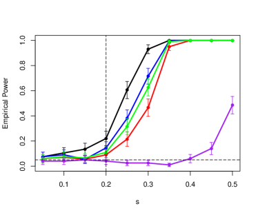
(a) $\beta=0.2$

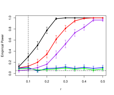
(b) $\beta=0.6$

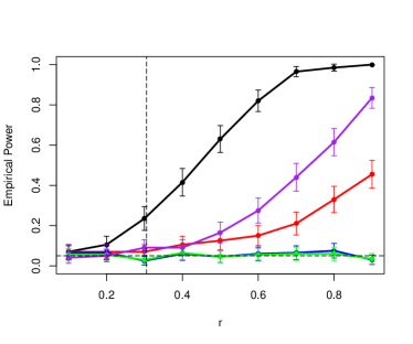
(c) $\beta=0.8$

Figure 1: Empirical power comparison with 95% error bars for the likelihood ratio test (black), the two-sample higher criticism test (red), the Wilcoxon test (blue), the two-sample Kolmogorov-Smirnov test (green) and the tail-run test (purple). 1(a) Dense regime where $\beta=0.2$. 1(b) Moderately sparse regime where $\beta=0.6$. 1(c) Very sparse regime where $\beta=0.8$. The horizontal line marks the level (set at 0.05) and the vertical line marks the asymptotic detection boundary derived earlier. The sample size is $m=n=10^{5}$ and the power curves and error bars are based on 200 replications.

Double-exponential mixture model

In this model, $F$ is double-exponential with variance 1. The simulation results are reported in Figure 2. The results are largely congruent with our theory.

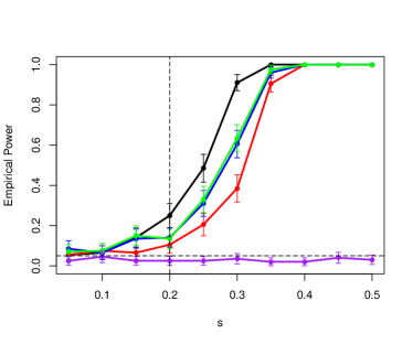
(a) $\beta=0.2$

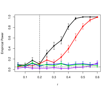
(b) $\beta=0.6$

Figure 2: Empirical power comparison with 95% error bars for the likelihood ratio test (black), the two-sample higher criticism test (red), the Wilcoxon test (blue), the two-sample Kolmogorov-Smirnov test (green) and the tail-run test (purple). 1(a) Dense regime where $\beta=0.2$. 1(b) Moderately sparse regime where $\beta=0.6$. 1(c) Very sparse regime where $\beta=0.8$. The horizontal line marks the level (set at 0.05) and the vertical line marks the asymptotic detection boundary derived earlier. The sample size is $m=n=10^{5}$ and the power curves and error bars are based on 200 replications.

References

• Arias-Castro and Huang [2020] E. Arias-Castro and R. Huang. The sparse variance contamination model. Statistics, 54(5):1081–1093, 2020. doi: 10.1080/02331888.2020.1823394.
• Arias-Castro and Wang [2016] E. Arias-Castro and M. Wang. Distribution-free tests for sparse heterogeneous mixtures. TEST, 26(1):71–94, 2016.
• Arias-Castro and Wang [2018] E. Arias-Castro and M. Wang. Distribution-free tests for sparse heterogeneous mixtures. arXiv preprint arXiv:1308.0346, 2018.
• Cai and Wu [2014] T. T. Cai and Y. Wu. Optimal detection of sparse mixtures against a given null distribution. IEEE Transactions on Information Theory, 60(4):2217–2232, 2014.
• Canner [1975] P. L. Canner. A simulation study of one-and two-sample kolmogorov-smirnov statistics with a particular weight function. Journal of the American Statistical Association, 70(349):209–211, 1975.
• Conover and Salsburg [1988] W. J. Conover and D. S. Salsburg. Locally most powerful tests for detecting treatment effects when only a subset of patients can be expected to “respond” to treatment. Biometrics, 44:189–196, 1988.
• Donoho and Jin [2004] D. Donoho and J. Jin. Higher criticism for detecting sparse heterogeneous mixtures. The Annals of Statistics, 32(3):962–994, 2004.