Full-Space Approach to Aerodynamic Shape Optimization

Abstract

Aerodynamic shape optimization (ASO) involves finding an optimal surface while constraining a set of nonlinear partial differential equations (PDE). The conventional approaches use quasi-Newton methods operating in the reduced-space, where the PDE constraints are eliminated at each design step by decoupling the flow solver from the optimizer. Conversely, the full-space Lagrange-Newton-Krylov-Schur (LNKS) approach couples the design and flow iteration by simultaneously minimizing the objective function and improving feasibility of the PDE constraints, which requires less iterations of the forward problem. Additionally, the use of second-order information leads to a number of design iterations independent of the number of control variables. We discuss the necessary ingredients to build an efficient LNKS ASO framework as well as the intricacies of their implementation. The LNKS approach is then compared to reduced-space approaches on a benchmark two-dimensional test case using a high-order discontinuous Galerkin method to discretize the PDE constraint.

1 Introduction

The field of aerodynamic shape optimization (ASO) is at a stage where complete aircraft [1, 2, 3, 4] and engine [5, 6] configurations can be designed through numerical optimization. As a result, increasingly complex geometries lead to ever increasing computational grids. While the number of control variables for shape optimization is currently in the order of tens or hundreds, the need for higher fidelity simulations is requiring the convergence of larger than ever discretized systems of partial differential equations (PDE). It is therefore advantageous to require a valid flow solution as infrequently as possible throughout the design process.

There are two ways to reduce the number of linear systems to be solved: decrease the number of design cycles or lower the number of linear systems to be solved within each design cycle. While current reduced-space quasi-Newton optimization frameworks can evaluate first-order sensitivities independently of the problem size through the adjoint method [7], the number of design cycles required to converge still increases proportionally to the number of control variables as more quasi-Newton updates are needed to correctly approximate the Hessian. Additionally, the reduced-space approach typically performs multiple iterations of the flow solver until full convergence of the PDE constraint, although tolerances on the flow residuals have been derived to maintain the same Q-convergence rate of the optimization problem [8].

Using Newton iterations within the reduced-space allows the optimizer to converge independently of the control variables size at the detriment of a higher cost within each cycle. While second-order adjoints [9, 10, 11] allow the Hessian to be computed at a cost proportional to the number of control variables, we have basically shifted the work dependence on the control dimensions from the outer iteration to the inner iteration. Hessian approximations [12, 13, 14] have been formulated to reduce its prohibitive cost and have demonstrated significant convergence improvement. Another possible solution is to solve the reduced system using Krylov subspace methods, which only require Hessian-vector products, at the cost of two linear solves per Krylov iteration [15, 16, 17]. However, the number of Krylov iterations required would scale with the size of the reduced system.

The full-space Lagrange-Newton-Krylov-Schur (LNKS) from Biros and Ghattas [18, 19] framework hopes to achieve convergence independent of problem size if the user can provide optimal preconditioners of the forward problem, dual problem, and reduced-Hessian. However, its implementation on complex problems have been challenging since the optimization framework must be able to store and manipulate parallelized discretizations rather than letting a blackbox solver handle the parallelization. For example, popular packages in the ASO community, such as SNOPT [20], NLPQLP [21], or IPOpt [22] cannot be used to implement LNKS. Apart from a quasi-one dimensional implementation [23, 17], the use of a Newton-based full-space approach has yet to be achieved in ASO on a larger scale.

In the present work, we define the different existing frameworks, and the cost associated with their sensitivities requirements. A description of the ingredients necessary to implement LNKS within an ASO framework is then provided. The resulting preconditioned systems in A and re-derived in C amend the original work [18]. Despite the differences, the eigenvalue spectra of the preconditioned systems shown in B coincide with the original preconditioner proposed in [18], and therefore do not affect the conclusions in [18].

We perform a dimensional analysis for an increasing number of control variables, and an increasing number of state variables to showcase the scalability of the various algorithms. Finally, we compare the full-space approach against reduced BFGS and reduced full-space methods similarly to [23] on an inverse design problem.

2 Optimization formulation

2.1 Problem statement

The ASO problem formulation can be stated as

$$\min_{\mathbf{u},{\boldsymbol{\alpha}}}\mathcal{F}(\mathbf{u},{\boldsymbol{\alpha}})\quad\text{subject to}\quad\boldsymbol{\mathcal{R}}(\mathbf{u},{\boldsymbol{\alpha}})=\mathbf{0},$$ (1)

where ${\boldsymbol{\alpha}}\in^{n}$ are the control variables , $\mathbf{u}\in^{m}$ are flow state variables , $\mathcal{F}:^{m}\times^{n}\to$ is the objective function, and $\boldsymbol{\mathcal{R}}:^{m}\times^{n}\to^{m}$ are the PDE constraints relating the geometry and flow solution.

The reduced and full-space approaches are implemented using the Trilinos’ Rapid Optimization Library (ROL) [24] which provides a modular large-scale parallel optimization framework.

2.2 Full-space

The full-space approach directly tackles the original problem in Eq. (1). To recover the optimality conditions, we form the Lagrangian function $\mathcal{L}$ as

$$\mathcal{L}(\mathbf{u},{\boldsymbol{\alpha}})\coloneqq\mathcal{F}(\mathbf{u},{\boldsymbol{\alpha}})+\boldsymbol{\lambda}^{T}\boldsymbol{\mathcal{R}}(\mathbf{u},{\boldsymbol{\alpha}}),$$ (2)

where $\boldsymbol{\lambda}\in^{m}$ are the adjoint variables. The first-order necessary optimality conditions, also known as the Karush-Kuhn-Tucker (KKT) conditions, are given by

$${\mathcal{L}_{\mathbf{u}}(\mathbf{u},{\boldsymbol{\alpha}})} ={\mathcal{F}_{\mathbf{u}}(\mathbf{u},{\boldsymbol{\alpha}})}+\boldsymbol{\lambda}^{T}{\boldsymbol{\mathcal{R}}_{\mathbf{u}}(\mathbf{u},{\boldsymbol{\alpha}})}=\mathbf{0},$$ (3a)

$${\mathcal{L}_{\boldsymbol{\alpha}}(\mathbf{u},{\boldsymbol{\alpha}})} ={\mathcal{F}_{\boldsymbol{\alpha}}(\mathbf{u},{\boldsymbol{\alpha}})}+\boldsymbol{\lambda}^{T}{\boldsymbol{\mathcal{R}}_{\boldsymbol{\alpha}}(\mathbf{u},{\boldsymbol{\alpha}})}=\mathbf{0},$$ (3b)

$${\mathcal{L}_{\boldsymbol{\lambda}}(\mathbf{u},{\boldsymbol{\alpha}})} =\boldsymbol{\mathcal{R}}(\mathbf{u},{\boldsymbol{\alpha}})=\mathbf{0}.$$ (3c)

The Newton iteration represented by the KKT system

$$\boldsymbol{\mathcal{K}}\mathbf{p}=\begin{bmatrix}\mathcal{L}_{\mathbf{u}\mathbf{u}}&\mathcal{L}_{\mathbf{u}{\boldsymbol{\alpha}}}&\boldsymbol{\mathcal{R}}_{\mathbf{u}}^{T}\\ \mathcal{L}_{{\boldsymbol{\alpha}}\mathbf{u}}&\mathcal{L}_{{\boldsymbol{\alpha}}{\boldsymbol{\alpha}}}&\boldsymbol{\mathcal{R}}_{{\boldsymbol{\alpha}}}^{T}\\ \boldsymbol{\mathcal{R}}_{\mathbf{u}}&\boldsymbol{\mathcal{R}}_{{\boldsymbol{\alpha}}}&\mathbf{0}\end{bmatrix}\begin{bmatrix}\mathbf{p}_{\mathbf{u}}\\ \mathbf{p}_{{\boldsymbol{\alpha}}}\\ \mathbf{p}_{\boldsymbol{\lambda}}\end{bmatrix}=-\begin{bmatrix}\mathcal{F}_{\mathbf{u}}+\boldsymbol{\lambda}^{T}\boldsymbol{\mathcal{R}}_{\mathbf{u}}\\ \mathcal{F}_{\boldsymbol{\alpha}}+\boldsymbol{\lambda}^{T}\boldsymbol{\mathcal{R}}_{\boldsymbol{\alpha}}\\ \boldsymbol{\mathcal{R}}\end{bmatrix},$$ (4)

where $\boldsymbol{\mathcal{K}}$ represents the KKT matrix and $\mathbf{p}$ is composed of the search directions $\mathbf{p}_{\mathbf{u}}=\mathbf{u}^{i+1}-\mathbf{u}^{i}$, $\mathbf{p}_{{\boldsymbol{\alpha}}}={\boldsymbol{\alpha}}^{i+1}-{\boldsymbol{\alpha}}^{i}$, and $\mathbf{p}_{\boldsymbol{\lambda}}=\boldsymbol{\lambda}^{i+1}-\boldsymbol{\lambda}^{i}$. Its assembly requires second-order sensitivities of the objective function and residuals to form the Hessian of the Lagrangian.

The dimensions of the KKT matrix ($2m+n$) on the left-hand side of Eq. (4) precludes direct factorization methods and is therefore solved using Krylov subspace methods such as GMRES [25]. Since it is a Newton-based method, the number of times this system needs to be solved is independent of the problem size. Furthermore, its solution only necessitates matrix-vector products, which involves no inversion of the forward or backward problem.

2.2.1 Full-space implementation

The search direction $\mathbf{p}$ is obtained by solving the KKT system Eq. (4) with FGMRES. A relative tolerance of 1.0e-6 is used to determine convergence of the linear system. The various preconditioners proposed by [18] are discussed in Sec. 3. A backtracking line-search also complements the algorithm for globalization purposes, where the augmented Lagrangian is used as the merit function as discussed in [19]

$$\mathcal{L}^{+}\coloneqq\mathcal{F}+\boldsymbol{\lambda}^{T}\boldsymbol{\mathcal{R}}+\frac{\mu}{2}\boldsymbol{\mathcal{R}}^{T}\boldsymbol{\mathcal{R}}=\mathcal{L}+\frac{\mu}{2}\boldsymbol{\mathcal{R}}^{T}\boldsymbol{\mathcal{R}},$$ (5)

with the penalty parameter $\mu$.

Our full-space implementation starts with a converged flow solution such that the flow residual is zero. While the full-space method does not postulate a feasible initial solution, it is performing Newton steps from the perspective of the steady-state flow solver. Therefore, starting from a free-stream solution resulted in inappropriate search directions, while a converged flow starts in the Newton ball of convergence.

However, the penalty parameter defined by Biros and Ghattas [19],

$$\mu_{\text{BG}}=\frac{\mathbf{p}_{\mathbf{u}}^{T}\mathcal{L}_{\mathbf{u}}+\mathbf{p}_{{\boldsymbol{\alpha}}}^{T}\mathcal{L}_{{\boldsymbol{\alpha}}}+\mathbf{p}_{\boldsymbol{\lambda}}^{T}\mathcal{L}_{\boldsymbol{\lambda}}+\delta}{\boldsymbol{\mathcal{R}}^{T}\left(\boldsymbol{\mathcal{R}}_{\mathbf{u}}\mathbf{p}_{\mathbf{u}}+\boldsymbol{\mathcal{R}}_{{\boldsymbol{\alpha}}}\mathbf{p}_{{\boldsymbol{\alpha}}}\right)}$$ (6)

is inversely proportional to the residual, $\boldsymbol{\mathcal{R}}$. Therefore, the initial converged flow solution, heavily penalized constraint violations, resulting in small step-lengths. Instead, we defined the penalty parameter to be inversely proportional to the norm of the Lagrangian gradient with respect to the control variables

$$\mu=\frac{c_{1}}{\|\mathcal{L}_{{\boldsymbol{\alpha}}}\|_{2}},$$ (7)

such that constraints are enforced to a greater extent as the optimization converges. A factor $c_{1}=0.01$ is used to scale the penalty parameter.

Previous one-shot methods leverage PDE solver technologies by using well-established explicit time-stepping schemes into their algorithm [26]. Since the current full-space approach is solved implicitly, pseudo-transient continuation [27] is used to increase the robustness of the algorithm. For steady-state flows, it is typical to cast the problem of solving

$$\boldsymbol{\mathcal{R}}(\mathbf{u},{\boldsymbol{\alpha}})=\mathbf{0}$$ (8)

into

$$\boldsymbol{\mathcal{M}}\dfrac{\partial\mathbf{u}}{\partial\tau}+\boldsymbol{\mathcal{R}}(\mathbf{u},{\boldsymbol{\alpha}})=\mathbf{0},$$ (9)

where $\boldsymbol{\mathcal{M}}$ represents the mass matrix and $\tau$ the pseudo-time. A backward Euler temporal discretization leads to

$$\left(\frac{\boldsymbol{\mathcal{M}}}{\Delta\tau}+\boldsymbol{\mathcal{R}}_{\mathbf{u}}\right)\left(\mathbf{u}^{i+1}-\mathbf{u}^{i}\right)=-\boldsymbol{\mathcal{R}},$$ (10)

which is analogous to solving the third row of Eq. (4) if $\Delta\tau\to\infty$ and $\mathbf{p}_{{\boldsymbol{\alpha}}}\to\mathbf{0}$

$$\boldsymbol{\mathcal{R}}_{\mathbf{u}}\mathbf{p}_{\mathbf{u}}=-\boldsymbol{\mathcal{R}}-\boldsymbol{\mathcal{R}}_{{\boldsymbol{\alpha}}}\mathbf{p}_{{\boldsymbol{\alpha}}}.$$ (11)

The Jacobian $\boldsymbol{\mathcal{R}}_{\mathbf{u}}$ is replaced by

$$\boldsymbol{\mathcal{R}}_{\mathbf{u}}^{+}=\boldsymbol{\mathcal{R}}_{\mathbf{u}}+\frac{\boldsymbol{\mathcal{M}}}{\Delta\tau},$$ (12)

where the pseudo-time step inversely scales with the square of the Lagrangian gradient norm

$$\Delta\tau=\frac{1}{\|\boldsymbol{\mathcal{R}}\|^{2}_{2}}.$$ (13)

While it is initially equivalent to solving a different set of constraints

$$\boldsymbol{\mathcal{R}}^{+}=\frac{\boldsymbol{\mathcal{M}}}{\Delta\tau}\mathbf{u}+\boldsymbol{\mathcal{R}},$$ (14)

the quadratically increasing time-step ensures that the continuation term disappears.

2.3 Reduced-space

Reduced-space approaches eliminate the constraints from the optimization problem by letting the flow solver satisfy the constraints at all times. Assuming that the flow Jacobian $\boldsymbol{\mathcal{R}}_{\mathbf{u}}\in^{m\times m}$ is invertible, the implicit function theorem states that there exists a function $\mathbf{w}:^{n}\to^{m}$ such that

$$\mathbf{w}({\boldsymbol{\alpha}})\equiv\mathbf{u}\quad\text{and}\quad\boldsymbol{\mathcal{R}}({\boldsymbol{\alpha}},\mathbf{w}({\boldsymbol{\alpha}}))=\mathbf{0}.$$ (15)

The residual’s total derivatives are then given by

$$\dfrac{\mathrm{d}\boldsymbol{\mathcal{R}}}{\mathrm{d}{\boldsymbol{\alpha}}}=\boldsymbol{\mathcal{R}}_{\mathbf{u}}\mathbf{w}_{\boldsymbol{\alpha}}+\boldsymbol{\mathcal{R}}_{\boldsymbol{\alpha}}=\mathbf{0},$$ (16)

where the sensitivity

$$\mathbf{w}_{\boldsymbol{\alpha}}=-\boldsymbol{\mathcal{R}}_{\mathbf{u}}^{-1}\boldsymbol{\mathcal{R}}_{\boldsymbol{\alpha}},$$ (17)

requires $n$ linear system solves.

In the reduced approach, a flow solver becomes responsible to ensure that the residual constraints are satisfied at every design cycle. For a nonlinear PDE, this involves multiple fixed-point iterations of the forward problem, which involves solving the flow Jacobian linear system multiple times until convergence.

The optimization problem can then be recast as the reduced formulation

$$\min_{{\boldsymbol{\alpha}}}\mathcal{F}({\boldsymbol{\alpha}},\mathbf{w}({\boldsymbol{\alpha}})).$$ (18)

2.3.1 Reduced gradient

The reduced gradient $\mathbf{g}_{z}$ of the objective function with respect to the control variables is given by

$$\mathbf{g}_{z}=\dfrac{\mathrm{d}\mathcal{F}}{\mathrm{d}{\boldsymbol{\alpha}}}=\mathcal{F}_{\boldsymbol{\alpha}}+\mathcal{F}_{\mathbf{u}}\mathbf{w}_{\boldsymbol{\alpha}}=\mathcal{F}_{\boldsymbol{\alpha}}-\mathcal{F}_{\mathbf{u}}\boldsymbol{\mathcal{R}}_{\mathbf{u}}^{-1}\boldsymbol{\mathcal{R}}_{\boldsymbol{\alpha}}=\mathcal{F}_{\boldsymbol{\alpha}}+\boldsymbol{\lambda}^{T}\boldsymbol{\mathcal{R}}_{\boldsymbol{\alpha}},$$ (19)

where the adjoint equation

$$\boldsymbol{\mathcal{R}}_{\mathbf{u}}^{T}\boldsymbol{\lambda}=-\mathcal{F}_{\mathbf{u}}^{T},$$ (20)

requires a single linear system solve to yield the dual state $\boldsymbol{\lambda}\in^{m}$ .

2.3.2 Reduced Hessian

Using a similar approach as Eqs. (16) and (17), we can derive the second-order residual and flow sensitivities

$$\dfrac{\mathrm{d}^{2}\boldsymbol{\mathcal{R}}}{\mathrm{d}{\boldsymbol{\alpha}}^{2}}=\mathbf{w}_{\boldsymbol{\alpha}}^{T}\boldsymbol{\mathcal{R}}_{\mathbf{u}\mathbf{u}}\mathbf{w}_{\boldsymbol{\alpha}}+\boldsymbol{\mathcal{R}}_{{\boldsymbol{\alpha}}\mathbf{u}}\mathbf{w}_{\boldsymbol{\alpha}}+\mathbf{w}_{\boldsymbol{\alpha}}^{T}\boldsymbol{\mathcal{R}}_{\mathbf{u}{\boldsymbol{\alpha}}}+\boldsymbol{\mathcal{R}}_{\mathbf{u}}\mathbf{w}_{{\boldsymbol{\alpha}}{\boldsymbol{\alpha}}}+\boldsymbol{\mathcal{R}}_{{\boldsymbol{\alpha}}{\boldsymbol{\alpha}}}=\mathbf{0},$$ (21)

such that

$$\mathbf{w}_{{\boldsymbol{\alpha}}{\boldsymbol{\alpha}}}=-\boldsymbol{\mathcal{R}}_{\mathbf{u}}^{-1}\left(\mathbf{w}_{\boldsymbol{\alpha}}^{T}\boldsymbol{\mathcal{R}}_{\mathbf{u}\mathbf{u}}\mathbf{w}_{\boldsymbol{\alpha}}+\boldsymbol{\mathcal{R}}_{{\boldsymbol{\alpha}}\mathbf{u}}\mathbf{w}_{\boldsymbol{\alpha}}+\mathbf{w}_{\boldsymbol{\alpha}}^{T}\boldsymbol{\mathcal{R}}_{\mathbf{u}{\boldsymbol{\alpha}}}+\boldsymbol{\mathcal{R}}_{{\boldsymbol{\alpha}}{\boldsymbol{\alpha}}}\right).$$ (22)

The second-order total derivatives of the objective function is then given by

$$\begin{split}\dfrac{\mathrm{d}^{2}\mathcal{F}}{\mathrm{d}{\boldsymbol{\alpha}}^{2}}&=\mathcal{F}_{{\boldsymbol{\alpha}}{\boldsymbol{\alpha}}}+\mathcal{F}_{{\boldsymbol{\alpha}}\mathbf{u}}\mathbf{w}_{\boldsymbol{\alpha}}+\mathbf{w}_{\boldsymbol{\alpha}}^{T}\mathcal{F}_{\mathbf{u}{\boldsymbol{\alpha}}}+\mathbf{w}_{\boldsymbol{\alpha}}^{T}\mathcal{F}_{\mathbf{u}\mathbf{u}}\mathbf{w}_{\boldsymbol{\alpha}}+\mathcal{F}_{\mathbf{u}}\mathbf{w}_{{\boldsymbol{\alpha}}{\boldsymbol{\alpha}}}\\ &=\mathcal{F}_{{\boldsymbol{\alpha}}{\boldsymbol{\alpha}}}+\mathcal{F}_{{\boldsymbol{\alpha}}\mathbf{u}}\mathbf{w}_{\boldsymbol{\alpha}}+\mathbf{w}_{\boldsymbol{\alpha}}^{T}\mathcal{F}_{\mathbf{u}{\boldsymbol{\alpha}}}+\mathbf{w}_{\boldsymbol{\alpha}}^{T}\mathcal{F}_{\mathbf{u}\mathbf{u}}\mathbf{w}_{\boldsymbol{\alpha}}\\ &\quad-\mathcal{F}_{\mathbf{u}}\boldsymbol{\mathcal{R}}_{\mathbf{u}}^{-1}\left(\mathbf{w}_{\boldsymbol{\alpha}}^{T}\boldsymbol{\mathcal{R}}_{\mathbf{u}\mathbf{u}}\mathbf{w}_{\boldsymbol{\alpha}}+\boldsymbol{\mathcal{R}}_{{\boldsymbol{\alpha}}\mathbf{u}}\mathbf{w}_{\boldsymbol{\alpha}}+\mathbf{w}_{\boldsymbol{\alpha}}^{T}\boldsymbol{\mathcal{R}}_{\mathbf{u}{\boldsymbol{\alpha}}}+\boldsymbol{\mathcal{R}}_{{\boldsymbol{\alpha}}{\boldsymbol{\alpha}}}\right)\\ &=\mathcal{F}_{{\boldsymbol{\alpha}}{\boldsymbol{\alpha}}}+\mathcal{F}_{{\boldsymbol{\alpha}}\mathbf{u}}\mathbf{w}_{\boldsymbol{\alpha}}+\mathbf{w}_{\boldsymbol{\alpha}}^{T}\mathcal{F}_{\mathbf{u}{\boldsymbol{\alpha}}}+\mathbf{w}_{\boldsymbol{\alpha}}^{T}\mathcal{F}_{\mathbf{u}\mathbf{u}}\mathbf{w}_{\boldsymbol{\alpha}}\\ &\quad+\boldsymbol{\lambda}^{T}\left(\mathbf{w}_{\boldsymbol{\alpha}}^{T}\boldsymbol{\mathcal{R}}_{\mathbf{u}\mathbf{u}}\mathbf{w}_{\boldsymbol{\alpha}}+\boldsymbol{\mathcal{R}}_{{\boldsymbol{\alpha}}\mathbf{u}}\mathbf{w}_{\boldsymbol{\alpha}}+\mathbf{w}_{\boldsymbol{\alpha}}^{T}\boldsymbol{\mathcal{R}}_{\mathbf{u}{\boldsymbol{\alpha}}}+\boldsymbol{\mathcal{R}}_{{\boldsymbol{\alpha}}{\boldsymbol{\alpha}}}\right)\\ &=\left(\mathcal{F}_{{\boldsymbol{\alpha}}{\boldsymbol{\alpha}}}+\boldsymbol{\lambda}^{T}\boldsymbol{\mathcal{R}}_{{\boldsymbol{\alpha}}{\boldsymbol{\alpha}}}\right)+\left(\mathcal{F}_{{\boldsymbol{\alpha}}\mathbf{u}}+\boldsymbol{\lambda}^{T}\boldsymbol{\mathcal{R}}_{{\boldsymbol{\alpha}}\mathbf{u}}\right)\mathbf{w}_{\boldsymbol{\alpha}}\\ &\quad+\mathbf{w}_{\boldsymbol{\alpha}}^{T}\left(\mathcal{F}_{\mathbf{u}{\boldsymbol{\alpha}}}+\boldsymbol{\lambda}^{T}\boldsymbol{\mathcal{R}}_{\mathbf{u}{\boldsymbol{\alpha}}}\right)+\mathbf{w}_{\boldsymbol{\alpha}}^{T}\left(\mathcal{F}_{\mathbf{u}\mathbf{u}}+\boldsymbol{\lambda}^{T}\boldsymbol{\mathcal{R}}_{\mathbf{u}\mathbf{u}}\right)\mathbf{w}_{\boldsymbol{\alpha}}\\ &=\mathcal{L}_{{\boldsymbol{\alpha}}{\boldsymbol{\alpha}}}+\mathcal{L}_{{\boldsymbol{\alpha}}\mathbf{u}}\mathbf{w}_{\boldsymbol{\alpha}}+\mathbf{w}_{\boldsymbol{\alpha}}^{T}\mathcal{L}_{\mathbf{u}{\boldsymbol{\alpha}}}+\mathbf{w}_{\boldsymbol{\alpha}}^{T}\mathcal{L}_{\mathbf{u}\mathbf{u}}\mathbf{w}_{\boldsymbol{\alpha}},\end{split}$$ (23)

which requires $n$ additional linear solves to obtain $\mathbf{w}_{\boldsymbol{\alpha}}$, assuming that $\boldsymbol{\lambda}$ has been pre-computed for the gradient. For ASO, the resulting matrix is usually small enough to directly be factorized. However, the $n$ additional linear solves quickly become prohibitive and some approximations can reduce its cost [12].

The reduced Hessian matrix will be abbreviated as

$$\mathcal{L}_{zz}\equiv\dfrac{\mathrm{d}^{2}\mathcal{F}}{\mathrm{d}{\boldsymbol{\alpha}}^{2}}.$$ (24)

In the case of inexact Newton-Krylov methods, where only the Hessian-vector products

$$\begin{split}\mathcal{L}_{zz}&=\mathcal{L}_{{\boldsymbol{\alpha}}{\boldsymbol{\alpha}}}\mathbf{v}+\mathcal{L}_{{\boldsymbol{\alpha}}\mathbf{u}}\mathbf{w}_{\boldsymbol{\alpha}}\mathbf{v}+\mathbf{w}_{\boldsymbol{\alpha}}^{T}\mathcal{L}_{\mathbf{u}{\boldsymbol{\alpha}}}\mathbf{v}+\mathbf{w}_{\boldsymbol{\alpha}}^{T}\mathcal{L}_{\mathbf{u}\mathbf{u}}\mathbf{w}_{\boldsymbol{\alpha}}\mathbf{v}\end{split}$$ (25)

are required, we can apply the Hessian at the cost of two linear system solves. The first solve forms

$$\mathbf{r}\coloneqq\mathbf{w}_{\boldsymbol{\alpha}}\mathbf{v}=\boldsymbol{\mathcal{R}}_{\mathbf{u}}^{-1}\left(\boldsymbol{\mathcal{R}}_{\boldsymbol{\alpha}}\mathbf{v}\right),$$ (26)

followed by

$$\begin{split}\mathbf{s}&\coloneqq\mathbf{w}_{\boldsymbol{\alpha}}^{T}\mathcal{L}_{\mathbf{u}{\boldsymbol{\alpha}}}\mathbf{v}+\mathbf{w}_{\boldsymbol{\alpha}}^{T}\mathcal{L}_{\mathbf{u}\mathbf{u}}\mathbf{w}_{\boldsymbol{\alpha}}\mathbf{v}\\ &=\boldsymbol{\mathcal{R}}_{\mathbf{u}}^{-T}\left(\boldsymbol{\mathcal{R}}_{{\boldsymbol{\alpha}}}^{T}\mathcal{L}_{\mathbf{u}{\boldsymbol{\alpha}}}\mathbf{v}+\boldsymbol{\mathcal{R}}_{{\boldsymbol{\alpha}}}^{T}\mathcal{L}_{\mathbf{u}\mathbf{u}}\mathbf{r}\right),\end{split}$$ (27)

to assemble into

$$\begin{split}\mathcal{L}_{zz}\mathbf{v}&=\mathcal{L}_{{\boldsymbol{\alpha}}{\boldsymbol{\alpha}}}\mathbf{v}+\mathcal{L}_{{\boldsymbol{\alpha}}\mathbf{u}}\mathbf{r}+\mathbf{s}.\end{split}$$ (28)

Hicken [17] provides tolerance bounds on those two solves such that superlinear convergence is observed for the optimization problem.

2.3.3 Reduced space implementation

The state variables $\mathbf{u}$ are obtained through backward Euler fixed-point iterations described in Eq. (10), followed by the adjoint linear solution to Eq. (20) before every control search direction computation.

The Newton search direction $\mathbf{p}_{{\boldsymbol{\alpha}}}$ is obtained through

$$\mathcal{L}_{zz}\mathbf{p}_{{\boldsymbol{\alpha}}}=-\mathbf{g}_{z}.$$ (29)

GMRES is used to solve the system by forming the matrix-vector products described in Eqs. (26-28) with an identity-initialized BFGS preconditioner. A relative tolerance of 1.0e-6 is used to determine convergence of the linear system. In the case of the quasi-Newton implementation, the reduced-Hessian is completely replaced with the BFGS approximation. A backtracking line-search also complements the algorithm for globalization purposes.

3 Full-space preconditioning

The convergence of Krylov solvers are directly related to the conditioning of the system whose convergence highly depends on the quality of the preconditioner. Biros and Ghattas [18] proposed preconditioners based on the reduced-space factorization. Their $\mathbf{P}_{4}$ and $\mathbf{P}_{2}$ preconditioners are defined as

$$\mathbf{P}_{4}=\begin{bmatrix}\mathcal{L}_{\mathbf{u}\mathbf{u}}\boldsymbol{\mathcal{R}}_{\mathbf{u}}^{-1}&\mathbf{0}&\mathbf{I}_{m}\\ \mathcal{L}_{{\boldsymbol{\alpha}}\mathbf{u}}\boldsymbol{\mathcal{R}}_{\mathbf{u}}^{-1}&\mathbf{I}_{n}&\boldsymbol{\mathcal{R}}_{{\boldsymbol{\alpha}}}^{T}\boldsymbol{\mathcal{R}}_{\mathbf{u}}^{-T}\\ \mathbf{I}_{m}&\mathbf{0}&\mathbf{0}\end{bmatrix}\begin{bmatrix}\boldsymbol{\mathcal{R}}_{\mathbf{u}}&\boldsymbol{\mathcal{R}}_{{\boldsymbol{\alpha}}}&\mathbf{0}\\ \mathbf{0}&\mathbf{B}_{z}&\mathbf{0}\\ \mathbf{0}&\mathbf{0}&\boldsymbol{\mathcal{R}}_{\mathbf{u}}^{T}\end{bmatrix}$$ (30)

$$\mathbf{P}_{2}=\begin{bmatrix}\mathbf{0}&\mathbf{0}&\mathbf{I}_{m}\\ \mathbf{0}&\mathbf{I}_{n}&\boldsymbol{\mathcal{R}}_{{\boldsymbol{\alpha}}}^{T}\boldsymbol{\mathcal{R}}_{\mathbf{u}}^{-T}\\ \mathbf{I}_{m}&\mathbf{0}&\mathbf{0}\end{bmatrix}\begin{bmatrix}\boldsymbol{\mathcal{R}}_{\mathbf{u}}&\boldsymbol{\mathcal{R}}_{{\boldsymbol{\alpha}}}&\mathbf{0}\\ \mathbf{0}&\mathbf{B}_{z}&\mathbf{0}\\ \mathbf{0}&\mathbf{0}&\boldsymbol{\mathcal{R}}_{\mathbf{u}}^{T}\end{bmatrix}=\begin{bmatrix}\mathbf{0}&\mathbf{0}&\boldsymbol{\mathcal{R}}_{\mathbf{u}}^{T}\\ \mathbf{0}&\mathbf{B}_{z}&\boldsymbol{\mathcal{R}}_{\boldsymbol{\alpha}}^{T}\\ \boldsymbol{\mathcal{R}}_{\mathbf{u}}&\boldsymbol{\mathcal{R}}_{\boldsymbol{\alpha}}&\mathbf{0}\end{bmatrix}$$ (31)

where $\mathbf{B}_{z}$ refers to an approximation of the reduced Hessian. The original Broyden-Fletcher-Goldfarb-Shanno (BFGS) quasi-Newton method [28, 29, 30, 31] will be used to update the preconditioner in this work. Note that the original version is used and not limited-memory BFGS [32] since it offers better convergence properties and the storage relative to the number of control variables is tractable in ASO.

The eigenvalue spectrum of $\mathbf{P}_{4}^{-1}$ and $\mathbf{P}_{2}^{-1}$ applied onto the KKT matrix $\boldsymbol{\mathcal{K}}$ from Eq. (4) will be the set of eigenvalues

$$\mathcal{E}(\mathbf{P}_{4}\boldsymbol{\mathcal{K}})=\mathcal{E}(\mathbf{P}_{2}\boldsymbol{\mathcal{K}})=\left\{\left\{\mathcal{E}(\mathbf{B}_{z}^{-1}\mathcal{L}_{zz})\right\},\left\{\mathbf{\mathbf{I}_{s}}\right\},\left\{\mathbf{\mathbf{I}_{s}}\right\}\right\}.$$ (32)

The application of $\mathbf{P}_{4}^{-1}$ requires 4 linear solves (two applications of $\boldsymbol{\mathcal{R}}_{\mathbf{u}}^{-1}$ and two applications of $\boldsymbol{\mathcal{R}}_{\mathbf{u}}^{-T}$) , while the application of $\mathbf{P}_{2}^{-1}$ only requires 2 linear solves while keeping the same system conditioning. By replacing the application of $\boldsymbol{\mathcal{R}}_{\mathbf{u}}^{-1}$ and $\boldsymbol{\mathcal{R}}_{\mathbf{u}}^{-T}$ by their respective preconditioners $\tilde{\boldsymbol{\mathcal{R}}}_{\mathbf{u}}^{-1}$ and $\tilde{\boldsymbol{\mathcal{R}}}_{\mathbf{u}}^{-T}$, we obtain the $\tilde{\mathbf{P}}_{4}^{-1}$ and $\tilde{\mathbf{P}}_{2}^{-1}$ preconditioners.

The Trilinos preconditioner library Ifpack [33] is used to form the flow Jacobian and adjoint flow Jacobian preconditioners. The preconditioner is an additive Schwarz domain decomposition method with 1 overlap between each subdomain and a threshold-based incomplete lower-upper factorization is used for each subdomain matrix with a fill ratio of 2, an absolute threshold of $1.0\text{\sc{e}-}4$, a relative threshold of 1.0, and a drop tolerance of $1.0\text{\sc{e}-}10$.

4 Flow constraints

The two-dimensional steady-state compressible Euler equations are used to model the flow and its PDEs in Cartesian coordinates $x_{1}$ and $x_{2}$ are described, using Einstein notation, by

$$\boldsymbol{\mathcal{R}}(\mathbf{u},\mathbf{x}({\boldsymbol{\alpha}}))=\dfrac{\partial\mathbf{f}_{i}(\mathbf{u},\mathbf{x}({\boldsymbol{\alpha}}))}{\partial x_{i}}=\mathbf{0},$$ (33)

where the conservative state vector $\mathbf{u}$, inviscid flux vector $\mathbf{f}_{i}$, are defined as,

$$\mathbf{u}=\begin{bmatrix}\rho&\rho v_{1}&\rho v_{2}&\rho E\end{bmatrix}^{T}$$ (34)

and

$$\mathbf{f}_{i}=\begin{bmatrix}\rho v_{i}&\rho v_{i}v_{1}+p\delta_{i1}&\rho v_{i}v_{2}+p\delta_{i2}&\rho Ev_{i}+pv_{i}\end{bmatrix}^{T}.$$ (35)

The density, velocities, Kronecker delta function, and total energy are respectively denoted as $\rho$, $v_{i}$, $\delta_{ij}$, and $E$. The total energy is given by $E=e+\frac{1}{2}(\|\mathbf{v}\|^{2})$. The pressure $p$ is determined by the equation of state

$$p=(\gamma-1)\rho\left(E-\|\mathbf{v}\|^{2}/2\right),$$ (36)

where $\gamma$ is the ratio of specific heats.

The equations are discretized using the weak form of the discontinuous Galerkin method [34] with a Roe flux [35]. The discretized equations are solved numerically using the Parallel High-Order Library for PDEs (PHiLiP) code which uses deal.II [36] as its backbone. Trilinos’ Sacado package [37] is used to automatically differentiate the discretized residual to obtain the first and second partial derivatives $\boldsymbol{\mathcal{R}}_{\mathbf{u}},\boldsymbol{\mathcal{R}}_{\mathbf{x}},\boldsymbol{\lambda}^{T}\boldsymbol{\mathcal{R}}_{\mathbf{u}\mathbf{u}},\boldsymbol{\lambda}^{T}\boldsymbol{\mathcal{R}}_{\mathbf{u}\mathbf{x}},$ and $\boldsymbol{\lambda}^{T}\boldsymbol{\mathcal{R}}_{{\boldsymbol{\alpha}}\mathbf{x}}$.

5 Design parametrization

While early works used the surface mesh points as control variables [7, 38], increasingly complex geometric constraints arose and more intuitive controls were needed. A popular method to parametrize the surface is to use free-form deformation (FFD) [39]. The displacements of the FFD control points are basically interpolated to locations within the FFD control box using Bézier curves. The surface of interest is surrounded by a FFD box defined by an origin $\mathbf{Q}$, and three vectors defining the parallepiped $\mathbf{S}$, $\mathbf{T}$, and $\mathbf{U}$. Any initial grid coordinate $\mathbf{x}_{\text{init}}=(x_{1},x_{2},x_{3})$ within the box has a corresponding local $(s,t,u)$ coordinate such that

$$\mathbf{x}_{\text{init}}=\mathbf{Q}+s\mathbf{S}+t\mathbf{T}+u\mathbf{U}.$$ (37)

The local coordinates can be obtained using some linear algebra

$$s=\frac{\mathbf{T}\times\mathbf{U}(\mathbf{x}_{\text{init}}-\mathbf{Q})}{\mathbf{T}\times\mathbf{U}\cdot\mathbf{S}},\quad t=\frac{\mathbf{S}\times\mathbf{U}(\mathbf{x}_{\text{init}}-\mathbf{Q})}{\mathbf{S}\times\mathbf{U}\cdot\mathbf{T}}\quad\text{and}\quad s=\frac{\mathbf{S}\times\mathbf{T}(\mathbf{x}_{\text{init}}-\mathbf{Q})}{\mathbf{S}\times\mathbf{T}\cdot\mathbf{U}}.$$ (38)

In two dimensions, it simplifies to

$$\mathbf{x}_{\text{init}}=\mathbf{Q}+s\mathbf{S}+t\mathbf{T},\quad s=\frac{(\mathbf{x}_{\text{init}}-\mathbf{Q})\cdot\mathbf{T}^{\perp}}{\mathbf{S}\cdot\mathbf{T}^{\perp}}\quad\text{and}\quad t=\frac{(\mathbf{x}_{\text{init}}-\mathbf{Q})\cdot\mathbf{S}^{\perp}}{\mathbf{T}\cdot\mathbf{S}^{\perp}}.$$ (39)

where the vector $\mathbf{v}=[v_{1},v_{2}]$ has its corresponding perpendicular vector $\mathbf{v}^{\perp}=[v_{2},-v_{1}]$. Control points $\mathbf{P}_{ijk}$ of the FFD parametrization are evenly spaced on the local $(s,t,u)$ coordinate such that for $(n_{s},n_{t},n_{u})$ control points in their respective directions

$$\mathbf{P}_{ijk}=\mathbf{Q}+\frac{i}{n_{s}}\boldsymbol{S}+\frac{j}{n_{t}}\boldsymbol{S}+\frac{k}{n_{u}}\boldsymbol{S}.$$ (40)

Finally, we can move the control points $\mathbf{P}_{ijk}$ and recover the new location of a point $(x,y,z)$ with corresponding local coordinates $(s,t,u)$ through the deformation function defined by the tensor product Bernstein polynomial

$$\mathbf{x}_{surf}=\sum_{i=0}^{n_{s}}\binom{n_{s}}{i}(1-s)^{n_{s}-i}s^{i}\left[\sum_{j=0}^{n_{t}}\binom{n_{t}}{j}(1-t)^{n_{t}-j}t^{j}\left[\sum_{k=0}^{n_{u}}\binom{n_{u}}{k}(1-u)^{n_{u}-k}u^{k}\mathbf{P}_{ijk}\right]\right].$$ (41)

A subset of the control points $\mathbf{P}_{ijk}$ will be chosen as the control variables ${\boldsymbol{\alpha}}$. Moreover, the necessary derivatives of the surface mesh points with respect to the control points are simply given by

$$\left(\dfrac{\partial\mathbf{x}_{surf}}{\partial\mathbf{P}_{ijk}}\right)_{ab}=\binom{n_{s}}{i}(1-s)^{n_{s}-i}s^{i}\binom{n_{t}}{j}(1-t)^{n_{t}-j}t^{j}\binom{n_{u}}{k}(1-u)^{n_{u}-k}u^{k}.$$ (42)

6 Volume mesh movement

Once the surface displacements have been recovered through the FFD, the volume mesh nodes need to be displaced to ensure a valid mesh. The high-order mesh is deformed using a linear elasticity mesh movement [40, 41, 42, 43] that propagates prescribed surface deformations into the domain.

The elastic equations with Dirichlet boundary conditions are described by

$$-\dfrac{\partial}{\partial x_{i}}\lambda\left(\dfrac{\partial(\Delta\mathbf{x_{vol}})_{j}}{\partial x_{j}}\right)-\dfrac{\partial}{\partial x_{j}}\left(\mu\dfrac{\partial(\Delta\mathbf{x_{vol}})_{j}}{\partial x_{i}}\right)-\dfrac{\partial}{\partial x_{j}}\left(\mu\dfrac{\partial(\Delta\mathbf{x_{vol}})_{i}}{\partial x_{j}}\right)=b_{i},\quad\mathbf{x}\in\boldsymbol{\Omega},$$ (43a)

$$\left(\Delta\mathbf{x_{vol}}\right)_{i}=\mathbf{M}_{ij}\left(\Delta\mathbf{x_{surf}}^{\text{BC}}\right)_{j},\quad\mathbf{x}\in{\partial\boldsymbol{\Omega}},$$ (43b)

where $(\Delta\mathbf{x_{vol}})$ represents the volume displacements, $(\Delta\mathbf{x_{surf}})$ represent the surface displacements, and $\mathbf{M}_{ij}$ maps the surface indices to their respective volume degree of freedom indices. Additionally, $\lambda$ and $\mu$ are the first and second Lamé parameters, and $\mathbf{b}$ are the external forces. The equation is discretized using the continuous Galerkin method since the node locations must be continuous across the elements. Since we only have boundary displacements, there are no external forces, such that $\mathbf{b}=\mathbf{0}$.

The Dirichlet boundary conditions are imposed by zero-ing the corresponding row of the stiffness matrix, setting the diagonal to 1, and the right-hand side to the Dirichlet value. We emphasize the importance of the described Dirichlet boundary conditions implementation since the resulting system to be solved becomes

$$\mathbf{S}\left(\Delta\mathbf{x_{vol}}\right)=\mathbf{M}\left(\Delta\mathbf{x_{surf}}^{\text{BC}}\right),$$ (44)

where $\mathbf{S}$ represents the stiffness matrix resulting from the discretization. Therefore, the mesh sensitivities are simply given by

$$\dfrac{\partial\mathbf{x_{vol}}}{\partial\mathbf{x_{surf}}}=\mathbf{S}^{-1}\mathbf{M}.$$ (45)

Since the mesh sensitivities require a linear solve every time either $\mathcal{F}_{{\boldsymbol{\alpha}}}$, $\mathcal{F}_{{\boldsymbol{\alpha}}\mathbf{u}}$, $\mathcal{F}_{\mathbf{u}{\boldsymbol{\alpha}}}$, $\mathcal{F}_{{\boldsymbol{\alpha}}{\boldsymbol{\alpha}}}$, $\boldsymbol{\mathcal{R}}_{{\boldsymbol{\alpha}}}$, $\boldsymbol{\mathcal{R}}_{{\boldsymbol{\alpha}}\mathbf{u}}$, $\boldsymbol{\mathcal{R}}_{\mathbf{u}{\boldsymbol{\alpha}}}$, or $\boldsymbol{\mathcal{R}}_{{\boldsymbol{\alpha}}{\boldsymbol{\alpha}}}$ is applied onto a vector, storing the chain-ruled derivative at the cost of $n$ linear solves

$$\dfrac{\partial\mathbf{x_{vol}}}{\partial{\boldsymbol{\alpha}}}=\dfrac{\partial\mathbf{x_{vol}}}{\partial\mathbf{x_{surf}}}\dfrac{\partial\mathbf{x_{surf}}}{\partial{\boldsymbol{\alpha}}}=\mathbf{S}^{-1}\mathbf{M}\dfrac{\partial\mathbf{x_{surf}}}{\partial{\boldsymbol{\alpha}}}$$ (46)

will result in higher performance since the total number of the mesh sensitivity applications will likely exceed the number of control variables. Furthermore, since the control variables and mesh movement always stem from an original mesh, the chain-ruled sensitivities only have to be pre-processed once. However, the memory requirement will be equivalent to storing $n$ meshes.

7 Cost analysis

7.1 Residual cost

The analysis is done in $d$-dimensions for the weak form of DG discretizing the $s=d+2$ Euler equations. We use an arbitrary tensor-product basis of order $p$ for the solution, and a Gauss-Lobatto tensor-product basis of order $p$ for the grid. A total of $n_{p}=(p+1)^{d}$ basis are used to discretize the solution and mesh. The integral computations use $n_{p}$ cubature nodes and $n_{f}=(p+1)^{d-1}$ quadrature nodes. Although the solution and the grid are discretized through tensor-product bases, the current implementation does not use the more cost effective sum-factorization method [44].

The number of flops required to evaluate the domain contribution is around $(32n_{p}^{2}+45n_{p})$ in 2D and $(58n_{p}^{2}+121n_{p})$, in 3D as per D.1, whereas the surface contribution is around $(32n_{p}n_{f}+227n_{f})$ in 2D and $(48n_{p}n_{f}+299n_{f})$ in 3D as detailed in D.2. For a structured 1/2/3D mesh, there will be 1/2/3 times as many faces as there are elements. Therefore, we obtain a total residual cost of

$$W\left(\boldsymbol{\mathcal{R}}\right)=32n_{p}^{2}+45n_{p}+2(32n_{p}n_{f}+227n_{f})$$ (47)

or

$$W\left(\boldsymbol{\mathcal{R}}\right)=32(p+1)^{4}+64(p+1)^{3}+45(p+1)^{2}+454(p+1)$$ (48)

in 2D and

$$W\left(\boldsymbol{\mathcal{R}}\right)=58n_{p}^{2}+121n_{p}+3(48n_{p}n_{f}+299n_{f})$$ (49)

or

$$W\left(\boldsymbol{\mathcal{R}}\right)=58(p+1)^{6}+144(p+1)^{5}+121(p+1)^{3}+897(p+1)^{2}$$ (50)

flops in 3D, where $W\left(\,\right)$ denotes the total number of flops. The absolute flops count is tabulated in Table 1. Additionally, $W_{\boldsymbol{\mathcal{R}}}\left(\,\right)$ will be used to denote other type of operations relative to $\boldsymbol{\mathcal{R}}$ such that $W_{\boldsymbol{\mathcal{R}}}\left(\texttt{ops}\right)=W\left(\texttt{ops}\right)/W\left(\boldsymbol{\mathcal{R}}\right)$ and $W_{\boldsymbol{\mathcal{R}}}\left(\boldsymbol{\mathcal{R}}\right)=1$.

	d
p	2			3
1	$692$  $/$	$710$  $/$	$2112$	$4680$  $/$	$2732$  $/$	$12\,876$
2	$2997$  $/$	$1545$  $/$	$6087$	$45\,549$  $/$	$14\,355$  $/$	$88\,614$
3	$8912$  $/$	$2956$  $/$	$14\,824$	$245\,312$  $/$	$53\,936$  $/$	$407\,120$
4	$21\,125$  $/$	$5135$  $/$	$31\,395$	$921\,375$  $/$	$157\,475$  $/$	$1\,393\,800$

Table 1: Flops required to assemble the volume/face/total residual of a single cell.

7.2 Matrix-vector products

The flops necessary to evaluate the matrix-vector products of the Jacobian or the Hessians are directly proportional to the sparsity of those operators. However, the time required to effectuate those flops differ from the flops of the residual assembly. Through numerical tests, we determined that the flops associated with the matrix-vector products are approximately three times faster than the ones from the residual assembly. The incongruity between the number of flops and timings can have multiple causes such as memory accesses, cache locality, and SIMD optimizations, which will vary with the implementation of the residual assembly. Therefore, the absolute work $W\left(\right)$ and relative work $W_{\boldsymbol{\mathcal{R}}}\left(\right)$ in Table 3, 3, and 4 will be divided by 3 in the remainder of the paper to more accurately reflect the timings. The experimental timings used a single core of a Ryzen 2700X processor with DDR4-2933 MHz memory to compare the residual assembly with the sparse matrix-vector products within PHiLiP.

7.2.1 Jacobian-vector product

A matrix-vector product of an already formed matrix will only involve the non-zeros of the matrix. The number of nonzeros per row of $\boldsymbol{\mathcal{R}}_{\mathbf{u}}$ is equal to the cell stencil size times the number of degrees of freedom per cell

$$N_{nz}^{\boldsymbol{\mathcal{R}}_{\mathbf{u}}}(p,d)=(1+2d)(d+2)(p+1)^{d}.$$ (51)

Therefore, the residuals corresponding to one cell has $n_{p}s$ rows and $N^{\boldsymbol{\mathcal{R}}_{\mathbf{u}}}_{nz}(p,d)$ non-zero columns. The total flops required to form the block-row-vector product is given by

$$\begin{split}W\left(\texttt{vmult}\left(\boldsymbol{\mathcal{R}}_{\mathbf{u}}\mathbf{v}\right)\right)&=2n_{p}sN^{\boldsymbol{\mathcal{R}}_{\mathbf{u}}}_{nz}(p,d)\\ &=2n_{p}s(1+2d)(d+2)(p+1)^{d}\\ &=(4d^{3}+18d^{2}+24d+8)(p+1)^{2d}.\end{split}$$ (52)

	d
p	2		3
1	$2560$  $/$	$1.2$	$22\,400$  $/$	$1.7$
2	$12\,960$  $/$	$2.1$	$255\,150$  $/$	$2.9$
3	$40\,960$  $/$	$2.8$	$1\,433\,600$  $/$	$3.5$
4	$100\,000$  $/$	$3.2$	$5\,468\,750$  $/$	$3.9$

Table 2: Flops/Relative work required to assemble matrix-vector product $\texttt{vmult}\left(\boldsymbol{\mathcal{R}}_{\mathbf{u}}\mathbf{v}\right)$ when $\boldsymbol{\mathcal{R}}_{\mathbf{u}}$ has been assembled already. $W\left(\texttt{vmult}\left(\boldsymbol{\mathcal{R}}_{\mathbf{u}}\mathbf{v}\right)\right)/W_{\boldsymbol{\mathcal{R}}}\left(\texttt{vmult}\left(\boldsymbol{\mathcal{R}}_{\mathbf{u}}\mathbf{v}\right)\right)$

	d
p	2		3
1	$256$  $/$	$0.12$	$1920$  $/$	$0.15$
2	$1296$  $/$	$0.21$	$21\,870$  $/$	$0.25$
3	$4096$  $/$	$0.28$	$122\,880$  $/$	$0.30$
4	$10\,000$  $/$	$0.32$	$468\,750$  $/$	$0.34$

Table 3: Flops/Relative work required to assemble matrix-vector product $\texttt{vmult}\left(\boldsymbol{\mathcal{R}}_{\mathbf{x_{vol}}}\mathbf{v}\right)$ when $\boldsymbol{\mathcal{R}}_{\mathbf{x_{vol}}}$ has been assembled already. $W\left(\texttt{vmult}\left(\boldsymbol{\mathcal{R}}_{\mathbf{x_{vol}}}\mathbf{v}\right)\right)/W_{\boldsymbol{\mathcal{R}}}\left(\texttt{vmult}\left(\boldsymbol{\mathcal{R}}_{\mathbf{x_{vol}}}\mathbf{v}\right)\right)$

A similar analysis can be used to obtain $W\left(\texttt{vmult}\left(\boldsymbol{\mathcal{R}}_{\mathbf{x_{vol}}}\mathbf{v}\right)\right)$. This time, the cell’s corresponding residuals only depends on its own nodes. The resulting work is therefore

$$\begin{split}W\left(\texttt{vmult}\left(\boldsymbol{\mathcal{R}}_{\mathbf{x_{vol}}}\mathbf{v}\right)\right)&=2n_{p}sd(p+1)^{d}=(2d^{2}+4d)(p+1)^{2d}.\end{split}$$ (53)

The total and relative work $W\left(\right)$ and $W_{\boldsymbol{\mathcal{R}}}\left(\right)$ are tabulated in Table 3 and 3, which will be divided by 3 as previously explained. Furthermore, the flow and adjoint Jacobian preconditioner use an ILUT fill ratio of 2 (not to be confused with ILU(2)), it has twice as many nonzeros, and its application is therefore twice as expensive.

7.2.2 Hessian-vector product

The dual-weighted residual Hessian block $\boldsymbol{\lambda}^{T}\boldsymbol{\mathcal{R}}_{\mathbf{u}\mathbf{u}}$ has the same sparsity pattern as $\boldsymbol{\mathcal{R}}_{\mathbf{u}}$ and therefore has the same matrix-vector product cost as described in Table 3. Similarly, the blocks $\boldsymbol{\lambda}^{T}\boldsymbol{\mathcal{R}}_{\mathbf{u}\mathbf{x_{vol}}}$ and $\boldsymbol{\lambda}^{T}\boldsymbol{\mathcal{R}}_{\mathbf{x_{vol}}\mathbf{u}}$ have the same sparsity pattern as $\boldsymbol{\mathcal{R}}_{\mathbf{x_{vol}}}$ and the same matrix-vector product cost described in Table 3. Finally, the matrix-vector product cost of $\boldsymbol{\lambda}^{T}\boldsymbol{\mathcal{R}}_{\mathbf{x_{vol}}\mathbf{x_{vol}}}$ listed in Table 4 is $d/(d+2)$ times the matrix-vector product cost of $\boldsymbol{\lambda}^{T}\boldsymbol{\mathcal{R}}_{\mathbf{u}\mathbf{x_{vol}}}$ since it contains less rows.

	d
p	2		3
1	$128$  $/$	$0.06$	$1152$  $/$	$0.09$
2	$648$  $/$	$0.11$	$13\,122$  $/$	$0.15$
3	$2048$  $/$	$0.14$	$73\,728$  $/$	$0.18$
4	$5000$  $/$	$0.16$	$281\,250$  $/$	$0.20$

Table 4: Flops/Relative work required to assemble matrix-vector product $\texttt{vmult}\left(\boldsymbol{\mathcal{R}}_{\mathbf{x_{vol}}\mathbf{x_{vol}}}\mathbf{v}\right)$ when $\boldsymbol{\mathcal{R}}_{\mathbf{x_{vol}}\mathbf{x_{vol}}}$ has been assembled already. $W\left(\texttt{vmult}\left(\boldsymbol{\mathcal{R}}_{\mathbf{x_{vol}}\mathbf{x_{vol}}}\mathbf{v}\right)\right)/W_{\boldsymbol{\mathcal{R}}}\left(\texttt{vmult}\left(\boldsymbol{\mathcal{R}}_{\mathbf{x_{vol}}\mathbf{x_{vol}}}\mathbf{v}\right)\right)$

7.3 Automatic differentiation

7.3.1 Forward and reverse work

Given the work required to assemble the residual $W\left(\boldsymbol{\mathcal{R}}\right)$ and a seed matrix $\mathbf{S}\in^{q\times k}$, where $q$ represents the number of independent variables and $k$ represents the number of columns on which to apply the residual derivative, a time complexity analysis of automatic differentiation [45] shows that the relative work $W_{\boldsymbol{\mathcal{R}}}\left(\boldsymbol{\mathcal{R}}_{\mathbf{u}}\mathbf{S}\right)$ of the vector forward mode is given by

$$1+k\leq W_{\boldsymbol{\mathcal{R}}}\left(\boldsymbol{\mathcal{R}}_{\mathbf{u}}\mathbf{S}\right)\leq 1.5+k,$$ (54)

where the range depends on the cost of memory access. The lower relative complexity occurs when the residual assembly is memory-bound, whereas the upper bound occurs when the residual assembly is compute-bound. For the remainder of this paper, we use an average $W_{\boldsymbol{\mathcal{R}}}\left(\boldsymbol{\mathcal{R}}_{\mathbf{u}}\mathbf{S}\right)\approx 1.25+k$. The vector reverse mode’s relative work $W_{\boldsymbol{\mathcal{R}}}\left(\mathbf{S}^{T}\boldsymbol{\mathcal{R}}_{\mathbf{u}}\right)$ is given by

$$1+2k\leq W_{\boldsymbol{\mathcal{R}}}\left(\mathbf{S}^{T}\boldsymbol{\mathcal{R}}_{\mathbf{u}}\right)\leq 1.5+2.5k$$ (55)

as derived in [45]. For the remainder of this paper, we use an average $W_{\boldsymbol{\mathcal{R}}}\left(\mathbf{S}^{T}\boldsymbol{\mathcal{R}}_{\mathbf{u}}\right)\approx 1.25+2.25k$.

7.3.2 Matrix-free product

If only a Jacobian-vector product is needed, then $k=1$ and

$$W_{\boldsymbol{\mathcal{R}}}\left(\boldsymbol{\mathcal{R}}_{\mathbf{u}}\mathbf{S}\right)=2.25.$$ (56)

The same applies to the mesh Jacobian since the AD relative cost only depends on the number of columns the derivative is applied onto such that

$$W_{\boldsymbol{\mathcal{R}}}\left(\boldsymbol{\mathcal{R}}_{\mathbf{x_{vol}}}\mathbf{S}\right)=2.25.$$ (57)

Similarly, the transposed versions with $k=1$ in the reverse mode results in

$$W_{\boldsymbol{\mathcal{R}}}\left(\mathbf{S}^{T}\boldsymbol{\mathcal{R}}_{\mathbf{u}}\right)=W_{\boldsymbol{\mathcal{R}}}\left(\mathbf{S}^{T}\boldsymbol{\mathcal{R}}_{\mathbf{x_{vol}}}\right)=3.5.$$ (58)

In the case of the dual-weighted residual Hessian, we simply use the reverse mode to first evaluate the dual-weighted Jacobian

$$W_{\boldsymbol{\mathcal{R}}}\left(\boldsymbol{\lambda}^{T}\boldsymbol{\mathcal{R}}_{\mathbf{u}}\right)=W_{\boldsymbol{\mathcal{R}}}\left(\boldsymbol{\lambda}^{T}\boldsymbol{\mathcal{R}}_{\mathbf{x_{vol}}}\right)=3.5.$$ (59)

The forward mode is then applied onto the seed vector with $k=1$ to multiply the above cost by 2.25.

$$\begin{split}W_{\boldsymbol{\mathcal{R}}}\left(\boldsymbol{\lambda}^{T}\boldsymbol{\mathcal{R}}_{\mathbf{u}\mathbf{u}}\mathbf{S}\right)&=W_{\boldsymbol{\mathcal{R}}}\left(\boldsymbol{\lambda}^{T}\boldsymbol{\mathcal{R}}_{\mathbf{u}\mathbf{x_{vol}}}\mathbf{S}\right)\\ &=W_{\boldsymbol{\mathcal{R}}}\left(\boldsymbol{\lambda}^{T}\boldsymbol{\mathcal{R}}_{\mathbf{x_{vol}}\mathbf{u}}\mathbf{S}\right)\\ &=W_{\boldsymbol{\mathcal{R}}}\left(\boldsymbol{\lambda}^{T}\boldsymbol{\mathcal{R}}_{\mathbf{x_{vol}}\mathbf{x_{vol}}}\mathbf{S}\right)\\ &=7.875.\end{split}$$ (60)

7.4 Forming the derivatives

While matrix-free preconditioners for DG are in development [46, 47], more standard algorithms, such as ILU, require the explicit matrix to be available. To build those derivatives, we simply have to apply the forward mode onto a seed matrix $\mathbf{S}$ with columns formed by the standard bases corresponding to independent variables.

In the case of the volume work, the number of independent variables are the number of degrees of freedom within the cell $k=(d+2)(p+1)^{d}$. For the face computations, the two neighbouring cells’ degrees of freedom are the independent variables, totalling $k=2(d+2)(p+1)^{d}$ columns of $\mathbf{S}$. The relative work $W_{\boldsymbol{\mathcal{R}}}\left(\boldsymbol{\mathcal{R}}_{\mathbf{u}}\right)$ therefore changes with the dimension and polynomial degree and is given by Table 6. A similar analysis can be performed on $W_{\boldsymbol{\mathcal{R}}}\left(\boldsymbol{\mathcal{R}}_{\mathbf{x_{vol}}}\right)$ by only using its own nodes to count the number of independent variables to obtain Table 6.

	d
p	2	3
1	$28.0$	$66.7$
2	$55.5$	$201.9$
3	$90.8$	$448.4$
4	$134.0$	$838.1$

Table 5: Relative work to assemble the flow Jacobian explicitly $W_{\boldsymbol{\mathcal{R}}}\left(\boldsymbol{\mathcal{R}}_{\mathbf{u}}\right)$ using AD.

	d
p	2	3
1	$9.2$	$25.2$
2	$19.2$	$82.2$
3	$33.2$	$193.2$
4	$51.2$	$376.2$

Table 6: Relative work to assemble the mesh Jacobian explicitly $W_{\boldsymbol{\mathcal{R}}}\left(\boldsymbol{\mathcal{R}}_{\mathbf{x_{vol}}}\right)$ using AD.

When it comes to finding the cost to form the dual-weighted residual Hessian blocks, we can start with the cost from Eq. (59). The seed matrix in Eq. (60) is then the same as the ones described to form $\boldsymbol{\mathcal{R}}_{\mathbf{u}}$ and $\boldsymbol{\mathcal{R}}_{\mathbf{x_{vol}}}$. As a result, the costs of assembling the dual-weighted residual Hessian blocks are

$$W_{\boldsymbol{\mathcal{R}}}\left(\boldsymbol{\lambda}^{T}\boldsymbol{\mathcal{R}}_{\mathbf{u}\mathbf{u}}\right)=W_{\boldsymbol{\mathcal{R}}}\left(\boldsymbol{\lambda}^{T}\boldsymbol{\mathcal{R}}_{\mathbf{u}}\right)\times W_{\boldsymbol{\mathcal{R}}}\left(\boldsymbol{\mathcal{R}}_{\mathbf{u}}\right)=3.5W_{\boldsymbol{\mathcal{R}}}\left(\boldsymbol{\mathcal{R}}_{\mathbf{u}}\right),$$ (61)

$$\begin{split}W_{\boldsymbol{\mathcal{R}}}\left(\boldsymbol{\lambda}^{T}\boldsymbol{\mathcal{R}}_{\mathbf{u}\mathbf{x_{vol}}}\right)&=W_{\boldsymbol{\mathcal{R}}}\left(\boldsymbol{\lambda}^{T}\boldsymbol{\mathcal{R}}_{\mathbf{x_{vol}}\mathbf{x_{vol}}}\right)\\ &=W_{\boldsymbol{\mathcal{R}}}\left(\boldsymbol{\lambda}^{T}\boldsymbol{\mathcal{R}}_{\mathbf{x_{vol}}}\right)\times W_{\boldsymbol{\mathcal{R}}}\left(\boldsymbol{\mathcal{R}}_{\mathbf{x_{vol}}}\right)\\ &=3.5W_{\boldsymbol{\mathcal{R}}}\left(\boldsymbol{\mathcal{R}}_{\mathbf{x_{vol}}}\right).\end{split}$$ (62)

Note that $W_{\boldsymbol{\mathcal{R}}}\left(\boldsymbol{\lambda}^{T}\boldsymbol{\mathcal{R}}_{\mathbf{u}\mathbf{x_{vol}}}\right)$ can be assembled more cheaply than $W_{\boldsymbol{\mathcal{R}}}\left(\boldsymbol{\lambda}^{T}\boldsymbol{\mathcal{R}}_{\mathbf{x_{vol}}\mathbf{u}}\right)$ and they are simply a transpose of each other.

	d
p	2	3
1	$98.0$	$233.5$
2	$194.3$	$706.5$
3	$317.7$	$1569.5$
4	$468.9$	$2933.3$

Table 7: Relative work to assemble the dual-weighted residual Hessian explicitly with second order state variables derivatives $W_{\boldsymbol{\mathcal{R}}}\left(\boldsymbol{\lambda}^{T}\boldsymbol{\mathcal{R}}_{\mathbf{u}\mathbf{u}}\right)$ using AD.

	d
p	2	3
1	$32.4$	$88.4$
2	$67.4$	$287.9$
3	$116.4$	$676.4$
4	$179.4$	$1316.9$

Table 8: Relative work to assemble the dual-weighted residual Hessian explicitly with a mesh derivative $W_{\boldsymbol{\mathcal{R}}}\left(\boldsymbol{\lambda}^{T}\boldsymbol{\mathcal{R}}_{\mathbf{u}\mathbf{x_{vol}}}\right)$ and $W_{\boldsymbol{\mathcal{R}}}\left(\boldsymbol{\lambda}^{T}\boldsymbol{\mathcal{R}}_{\mathbf{x_{vol}}\mathbf{x_{vol}}}\right)$ using AD.

7.5 Matrix-free versus forming the matrices

The matrix-free approaches to evaluate Jacobian-vector and transpose-Jacobian-vector products has a constant relative cost of 2.25 and 3.5 residual evaluations. The matrix-free dual-weighted residual Hessian-vector products also have a relative constant complexity of 7.875. Those matrix-free products are more expensive than performing the matrix-vector product when the matrix has been pre-assembled. It is not obvious whether it is worth investing a large amount of time once to save flops by performing the matrix-vector products with a pre-assembled matrix, rather than forming the matrix-vector products on-the-fly through AD. In the case of the flow Jacobian $\boldsymbol{\mathcal{R}}_{\mathbf{u}}$, the explicit matrix is required to form the preconditioner of the forward and adjoint problem.

However, for $\boldsymbol{\mathcal{R}}_{\mathbf{x_{vol}}}$, $\boldsymbol{\lambda}^{T}\boldsymbol{\mathcal{R}}_{\mathbf{u}\mathbf{u}}$, $\boldsymbol{\lambda}^{T}\boldsymbol{\mathcal{R}}_{\mathbf{u}\mathbf{x_{vol}}}$, $\boldsymbol{\lambda}^{T}\boldsymbol{\mathcal{R}}_{\mathbf{x_{vol}}\mathbf{u}}$, and $\boldsymbol{\lambda}^{T}\boldsymbol{\mathcal{R}}_{\mathbf{x_{vol}}\mathbf{x_{vol}}}$, we determine how many times the matrices have to be used by dividing the initial cost by the cost savings

$$C\left(\boldsymbol{\mathcal{R}}_{\mathbf{x_{vol}}}\right)=\frac{W_{\boldsymbol{\mathcal{R}}}\left(\boldsymbol{\mathcal{R}}_{\mathbf{x_{vol}}}\right)}{\left(W_{\boldsymbol{\mathcal{R}}}\left(\texttt{vmult}\left(\boldsymbol{\mathcal{R}}_{\mathbf{x_{vol}}}\mathbf{v}\right)\right)-W_{\boldsymbol{\mathcal{R}}}\left(\boldsymbol{\mathcal{R}}_{\mathbf{x_{vol}}}\mathbf{v}\right)\right)}.$$ (63)

The number of times the matrix-products have to be formed to recover the initial cost are listed in Tables 10–12. The optimization results in the following section are in 2D up to $p=3$. Since the matrix assembly cost is recouped after very few matrix-vector products and the total number of matrix-vector products required is not known a priori, the derivative operators are always fully formed rather than assembling the matrix-vector product on-the-fly.

	d
p	2	3
1	$2$	$6$
2	$4$	$19$
3	$8$	$45$
4	$12$	$88$

Table 9: Number of times we need the matrix-vector product $\boldsymbol{\mathcal{R}}_{\mathbf{x_{vol}}}\mathbf{v}$ to warrant forming the matrix explicitly instead of assembling the matrix-product on-the-fly with AD. Its assembly cost has been divided by 2 since once assembled, it can be used for the required transpose matrix-vector product.

	d
p	2	3
1	$13$	$32$
2	$27$	$102$
3	$46$	$234$
4	$69$	$447$

Table 10: Number of times we need the matrix-vector product $\boldsymbol{\mathcal{R}}_{\mathbf{u}\mathbf{u}}\mathbf{v}$ to warrant forming the matrix explicitly instead of assembling the matrix-product on-the-fly with AD.

	d
p	2	3
1	$2$	$6$
2	$4$	$18$
3	$7$	$44$
4	$12$	$85$

Table 11: Number of times we need the matrix-vector product $\boldsymbol{\mathcal{R}}_{\mathbf{u}\mathbf{x_{vol}}}\mathbf{v}$ to warrant forming the matrix explicitly instead of assembling the matrix-product on-the-fly with AD. Its assembly cost has been divided by 2 since once assembled, it can be used for the required transpose matrix-vector product.

	d
p	2	3
1	$4$	$11$
2	$9$	$37$
3	$15$	$87$
4	$23$	$169$

Table 12: Number of times we need the matrix-vector product $\boldsymbol{\mathcal{R}}_{\mathbf{x_{vol}}\mathbf{x_{vol}}}\mathbf{v}$ to warrant forming the matrix explicitly instead of assembling the matrix-product on-the-fly with AD.

8 Results

8.1 Test case description

(a)

(b)

Figure 1: Gaussian bump pressure distribution and FFD control points

The benchmark problem is the inverse target optimization of an inviscid channel flow from the High Order CFD workshop [48]. The channel is defined on $(x,y)=([-1.5,1.5],[0,0.8])$ and the lower surface follows a Gaussian bump

$$y(x)=h\exp(-25x^{2}),$$ (64)

where $h=0.0625$ for the initial grid and $h=0.03125$ for the target grid as seen in Fig. 1. A FFD box is defined around the lower surface using $\mathbf{Q}=(-1.4,-0.1)$, $\boldsymbol{S}=(2.8,0)$, and $\boldsymbol{T}=(0,0.6)$. The control variables are the $y$-component of the FFD control points, excluding the left-most, right-most, and bottom points to ensure a valid grid.

We impose total pressure and total temperature at the inlet, as well as an inflow Mach number of 0.3, while a static pressure ratio is prescribed at the subsonic outlet. Characteristic boundary conditions as described in [49] are imposed implicitly. The objective function is defined as

$$\mathcal{F}(\mathbf{u},{\boldsymbol{\alpha}})=\int_{{\partial\boldsymbol{\Omega}}}\sum_{i}\left(u_{i}-u_{i}^{t}\right)^{2}\mathop{}\!\mathrm{d}{\partial\boldsymbol{\Omega}},$$ (65)

8.2 Verification

Since the test case is subsonic and the geometry is smooth the flow is isentropic. The $L_{2}$-norm of the entropy error is used to measure the solution accuracy.

$$E_{\text{entropy}}=\sqrt{\int_{\boldsymbol{\Omega}}\left(\frac{p}{p_{\infty}}\left(\frac{\rho_{\infty}}{\rho}\right)^{\gamma}-1\right)^{2}\mathop{}\!\mathrm{d}\boldsymbol{\Omega}}.$$ (66)

The entropy error should converge at a rate of $p+1$ for a DG discretization of order $p$ as seen in Table 13.

Degree $p$	Cells	Number of DoFs	$L_{2}$ entropy error	Rate
1	$64$	$1024$	5.73e-03	-
1	$256$	$4096$	1.30e-03	2.14
1	$1024$	$16\,384$	2.26e-04	2.53
1	$4096$	$65\,536$	4.30e-05	2.39
1	$16\,384$	$262\,144$	9.07e-06	2.25
2	$64$	$2304$	9.86e-04	-
2	$256$	$9216$	7.68e-05	3.68
2	$1024$	$36\,864$	7.19e-06	3.42
2	$4096$	$147\,456$	7.91e-07	3.18
2	$16\,384$	$589\,824$	9.34e-08	3.08
3	$64$	$4096$	1.57e-04	-
3	$256$	$16\,384$	1.03e-05	3.94
3	$1024$	$65\,536$	6.80e-07	3.91
3	$4096$	$262\,144$	5.07e-08	3.75
3	$16\,384$	$1\,048\,576$	3.23e-09	3.97

Table 13: Orders of accuracy table demonstrating $L_{2}$ norm of the entropy error diminishing at a rate of of $p+1$ for a discretization of order $p$.

8.3 Optimization results

The inverse design problem is solved using the full-space with various preconditioners, the reduced-space Newton, and the reduced-space quasi-Newton for various polynomial degrees ($p=1,2,3$, corresponding to $m=4000,9000,16000$ discretization degrees of freedom) and for various numbers of control variables ($n=20,40,60,80,100$). The entire set of results is concatenated in Table 14.

$n$	Cycles			Total Subits.			Avg. Subits./Cycle			Total Work			Avg. Work/Cycle
Full-space $\mathbf{P}_{4}$
20	$5$  $/$	$5$  $/$	$5$	$111$  $/$	$113$  $/$	$110$	$22.2$  $/$	$22.6$  $/$	$22.0$	$60\,453$  $/$	$129\,849$  $/$	$188\,277$	$12\,091$  $/$	$25\,970$  $/$	$37\,655$
40	$5$  $/$	$5$  $/$	$5$	$162$  $/$	$157$  $/$	$159$	$32.4$  $/$	$31.4$  $/$	$31.8$	$85\,696$  $/$	$178\,114$  $/$	$268\,069$	$17\,139$  $/$	$35\,623$  $/$	$53\,614$
60	$4$  $/$	$5$  $/$	$5$	$158$  $/$	$192$  $/$	$199$	$39.5$  $/$	$38.4$  $/$	$39.8$	$82\,837$  $/$	$217\,048$  $/$	$329\,648$	$20\,709$  $/$	$43\,410$  $/$	$65\,930$
80	$4$  $/$	$5$  $/$	$5$	$181$  $/$	$227$  $/$	$226$	$45.2$  $/$	$45.4$  $/$	$45.2$	$94\,181$  $/$	$253\,188$  $/$	$375\,115$	$23\,545$  $/$	$50\,638$  $/$	$75\,023$
100	$4$  $/$	$5$  $/$	$5$	$196$  $/$	$248$  $/$	$246$	$49.0$  $/$	$49.6$  $/$	$49.2$	$102\,381$  $/$	$277\,537$  $/$	$408\,023$	$25\,595$  $/$	$55\,507$  $/$	$81\,605$
Full-space $\mathbf{P}_{2}$
20	$5$  $/$	$5$  $/$	$5$	$129$  $/$	$132$  $/$	$130$	$25.8$  $/$	$26.4$  $/$	$26.0$	$33\,828$  $/$	$73\,457$  $/$	$107\,643$	$6766$  $/$	$14\,691$  $/$	$21\,529$
40	$5$  $/$	$5$  $/$	$5$	$188$  $/$	$181$  $/$	$188$	$37.6$  $/$	$36.2$  $/$	$37.6$	$48\,347$  $/$	$99\,804$  $/$	$153\,567$	$9669$  $/$	$19\,961$  $/$	$30\,713$
60	$4$  $/$	$5$  $/$	$5$	$179$  $/$	$220$  $/$	$227$	$44.8$  $/$	$44.0$  $/$	$45.4$	$46\,129$  $/$	$120\,854$  $/$	$184\,120$	$11\,532$  $/$	$24\,171$  $/$	$36\,824$
80	$4$  $/$	$5$  $/$	$5$	$204$  $/$	$258$  $/$	$263$	$51.0$  $/$	$51.6$  $/$	$52.6$	$52\,391$  $/$	$141\,722$  $/$	$212\,156$	$13\,098$  $/$	$28\,344$  $/$	$42\,431$
100	$4$  $/$	$5$  $/$	$5$	$225$  $/$	$281$  $/$	$282$	$56.2$  $/$	$56.2$  $/$	$56.4$	$57\,491$  $/$	$153\,734$  $/$	$227\,260$	$14\,373$  $/$	$30\,747$  $/$	$45\,452$
Full-space $\tilde{\mathbf{P}}_{4}$
20	$5$  $/$	$5$  $/$	$5$	$1158$  $/$	$1227$  $/$	$1325$	$231.6$  $/$	$245.4$  $/$	$265.0$	$7223$  $/$	$13\,634$  $/$	$19\,695$	$1445$  $/$	$2727$  $/$	$3939$
40	$5$  $/$	$5$  $/$	$5$	$1430$  $/$	$1563$  $/$	$1715$	$286.0$  $/$	$312.6$  $/$	$343.0$	$8640$  $/$	$16\,710$  $/$	$24\,329$	$1728$  $/$	$3342$  $/$	$4866$
60	$4$  $/$	$5$  $/$	$5$	$1308$  $/$	$1759$  $/$	$1887$	$327.0$  $/$	$351.8$  $/$	$377.4$	$7800$  $/$	$18\,505$  $/$	$26\,372$	$1950$  $/$	$3701$  $/$	$5274$
80	$4$  $/$	$5$  $/$	$5$	$1407$  $/$	$1955$  $/$	$2077$	$351.8$  $/$	$391.0$  $/$	$415.4$	$8316$  $/$	$20\,299$  $/$	$28\,627$	$2079$  $/$	$4060$  $/$	$5725$
100	$4$  $/$	$5$  $/$	$5$	$1493$  $/$	$2071$  $/$	$2252$	$373.2$  $/$	$414.2$  $/$	$450.4$	$8764$  $/$	$21\,361$  $/$	$30\,709$	$2191$  $/$	$4272$  $/$	$6142$
Full-space $\tilde{\mathbf{P}}_{2}$
20	$5$  $/$	$5$  $/$	$5$	$1199$  $/$	$1270$  $/$	$1370$	$239.8$  $/$	$254.0$  $/$	$274.0$	$4893$  $/$	$9296$  $/$	$13\,605$	$979$  $/$	$1859$  $/$	$2721$
40	$5$  $/$	$5$  $/$	$5$	$1496$  $/$	$1630$  $/$	$1776$	$299.2$  $/$	$326.0$  $/$	$355.2$	$5811$  $/$	$11\,250$  $/$	$16\,466$	$1162$  $/$	$2250$  $/$	$3293$
60	$4$  $/$	$5$  $/$	$5$	$1352$  $/$	$1830$  $/$	$1952$	$338.0$  $/$	$366.0$  $/$	$390.4$	$5161$  $/$	$12\,336$  $/$	$17\,706$	$1290$  $/$	$2467$  $/$	$3541$
80	$4$  $/$	$5$  $/$	$5$	$1453$  $/$	$2026$  $/$	$2147$	$363.2$  $/$	$405.2$  $/$	$429.4$	$5473$  $/$	$13\,400$  $/$	$19\,077$	$1368$  $/$	$2680$  $/$	$3815$
100	$4$  $/$	$5$  $/$	$5$	$1552$  $/$	$2161$  $/$	$2313$	$388.0$  $/$	$432.2$  $/$	$462.6$	$5779$  $/$	$14\,133$  $/$	$20\,249$	$1445$  $/$	$2827$  $/$	$4050$
160	$4$  $/$	$5$  $/$	$5$	$1721$  $/$	$2409$  $/$	$2628$	$430.2$  $/$	$481.8$  $/$	$525.6$	$6302$  $/$	$15\,480$  $/$	$22\,469$	$1575$  $/$	$3096$  $/$	$4494$
320	$4$  $/$	$5$  $/$	$5$	$2104$  $/$	$2668$  $/$	$2948$	$526.0$  $/$	$533.6$  $/$	$589.6$	$7486$  $/$	$16\,886$  $/$	$24\,723$	$1871$  $/$	$3377$  $/$	$4945$
640	$5$  $/$	$5$  $/$	$5$	$2920$  $/$	$3435$  $/$	$3477$	$584.0$  $/$	$687.0$  $/$	$695.4$	$10\,212$  $/$	$21\,050$  $/$	$28\,451$	$2042$  $/$	$4210$  $/$	$5690$
Reduced-space Newton
20	$4$  $/$	$4$  $/$	$4$	$68$  $/$	$67$  $/$	$65$	$17.0$  $/$	$16.8$  $/$	$16.2$	$21\,397$  $/$	$44\,526$  $/$	$64\,156$	$5349$  $/$	$11\,131$  $/$	$16\,039$
40	$4$  $/$	$4$  $/$	$4$	$100$  $/$	$101$  $/$	$103$	$25.0$  $/$	$25.2$  $/$	$25.8$	$29\,248$  $/$	$62\,060$  $/$	$93\,477$	$7312$  $/$	$15\,515$  $/$	$23\,369$
60	$4$  $/$	$4$  $/$	$4$	$128$  $/$	$126$  $/$	$126$	$32.0$  $/$	$31.5$  $/$	$31.5$	$35\,809$  $/$	$75\,482$  $/$	$111\,420$	$8952$  $/$	$18\,871$  $/$	$27\,855$
80	$4$  $/$	$4$  $/$	$4$	$142$  $/$	$147$  $/$	$149$	$35.5$  $/$	$36.8$  $/$	$37.2$	$39\,397$  $/$	$86\,220$  $/$	$129\,417$	$9849$  $/$	$21\,555$  $/$	$32\,354$
100	$4$  $/$	$4$  $/$	$4$	$162$  $/$	$163$  $/$	$161$	$40.5$  $/$	$40.8$  $/$	$40.2$	$44\,256$  $/$	$95\,040$  $/$	$139\,496$	$11\,064$  $/$	$23\,760$  $/$	$34\,874$
160	$4$  $/$	$4$  $/$	$4$	$193$  $/$	$202$  $/$	$206$	$48.2$  $/$	$50.5$  $/$	$51.5$	$52\,244$  $/$	$116\,218$  $/$	$174\,302$	$13\,061$  $/$	$29\,055$  $/$	$43\,575$
320	$4$  $/$	$4$  $/$	$4$	$246$  $/$	$253$  $/$	$264$	$61.5$  $/$	$63.2$  $/$	$66.0$	$65\,920$  $/$	$143\,962$  $/$	$221\,465$	$16\,480$  $/$	$35\,991$  $/$	$55\,366$
640	$4$  $/$	$4$  $/$	$4$	$336$  $/$	$359$  $/$	$346$	$84.0$  $/$	$89.8$  $/$	$86.5$	$87\,027$  $/$	$199\,590$  $/$	$285\,098$	$21\,757$  $/$	$49\,898$  $/$	$71\,274$
Reduced-space BFGS
20	$61$  $/$	$62$  $/$	$64$	$0$  $/$	$0$  $/$	$0$	$0.0$  $/$	$0.0$  $/$	$0.0$	$38\,967$  $/$	$82\,569$  $/$	$123\,860$	$639$  $/$	$1332$  $/$	$1935$
40	$78$  $/$	$74$  $/$	$72$	$0$  $/$	$0$  $/$	$0$	$0.0$  $/$	$0.0$  $/$	$0.0$	$51\,288$  $/$	$98\,358$  $/$	$128\,359$	$658$  $/$	$1329$  $/$	$1783$
60	$85$  $/$	$93$  $/$	$81$	$0$  $/$	$0$  $/$	$0$	$0.0$  $/$	$0.0$  $/$	$0.0$	$54\,183$  $/$	$119\,824$  $/$	$135\,045$	$637$  $/$	$1288$  $/$	$1667$
80	$76$  $/$	$81$  $/$	$76$	$0$  $/$	$0$  $/$	$0$	$0.0$  $/$	$0.0$  $/$	$0.0$	$51\,022$  $/$	$102\,596$  $/$	$126\,967$	$671$  $/$	$1267$  $/$	$1671$
100	$91$  $/$	$78$  $/$	$80$	$0$  $/$	$0$  $/$	$0$	$0.0$  $/$	$0.0$  $/$	$0.0$	$59\,764$  $/$	$92\,270$  $/$	$133\,987$	$657$  $/$	$1183$  $/$	$1675$

Table 14: Convergence summary of the various methods discussed. $\left(\cdot\right)/\left(\cdot\right)/\left(\cdot\right)$ are the data points given for $m=4000,9000,16000$.

The full-space framework is Newton-based and therefore converges independently of the control space size as seen in Fig. 2. Since the same KKT system is solved to the same tolerance for various preconditioners, the search directions should be relatively similar. Slight differences may occur since the preconditioner type will affect the accuracy of the various search direction components. For example, it is expected that the $\mathbf{P}_{4}$ preconditioner more accurately resolves the state and adjoint search directions, thus allowing a higher residual error in the control search direction. Conversely, the $\tilde{\mathbf{P}}_{2}$ would distribute the allowable error amongst all three directions.

The effectiveness of each preconditioner is observed in Fig. 4 & 5. As expected, the $\mathbf{P}_{4}$ and $\mathbf{P}_{2}$ preconditioners greatly reduces the number of Krylov iterations since the eigenvalue spectrum is composed of at most $(n+1)$ different values. In fact, Table 14 shows that increasing the number of state variables does not affect the average number of subiterations, which confirms that the eigenvalue spectra of those preconditioned systems only depends on the control variables. On the other hand, $\tilde{\mathbf{P}}_{4}$ and $\tilde{\mathbf{P}}_{2}$ requires many more subiterations, but still allows FGMRES to converge, whereas the unpreconditioned system solve simply stalls.

However, each application of $\mathbf{P}_{4}^{-1}$ and $\mathbf{P}_{2}^{-1}$ is much costlier than $\tilde{\mathbf{P}}_{4}^{-1}$ and $\tilde{\mathbf{P}}_{2}^{-1}$. The total amount of work required to converge is shown in Fig. 6. As the control space or the state space increases in size, the cost of the $\mathbf{P}_{4}$ preconditioned full-space, that excelled in subiterations, shows a significant increase in cost. Table 14 shows that when $\tilde{\mathbf{P}}_{2}$ is used, the work slowly increases as $m$ or $n$ increases although it required the most subiterations.

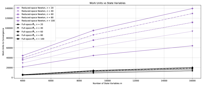
Figure 2: Full-space method convergence is independent of control variables size.

Figure 3: Reduced-space BFGS design cycles requires to converge. Note that the reduced-space Newton method requires a constant 4 design cycles regardless of $n$ or $m$.

Figure 4: Effectiveness of preconditioners on the number of FGMRES iterations required to solve the KKT system.

Figure 5: Full-space method total number of subiterations required to converge.

Figure 6: Full-space method work required to converge.

The quasi-Newton is compared against the Newton method in Fig. 7. The Newton method converges independently of the control space size just as the full-space method, whereas the BFGS method requires an increasing number of design cycles as seen Fig. 3. However, Table 14 shows that the number of subiterations within the Newton’s method linear solve increases as the eigenvalue spectrum widens. Looking at the total work to convergence in Fig. 8 gives a clearer picture. The reduced-space Newton method outperforms the quasi-Newton approach for lower numbers of control variables, but its cost becomes comparable around 100 control variables.

Figure 7: Reduced-space gradient convergence with design cycles.

Finally, we compare the reduced-space approach with the best performing full-space approach in Fig. 9. Additional data points at $n=160,320,640$ have been evaluated to observe the scaling of both algorithms. Unfortunately, the reduced-space BFGS algorithm fails to find a suitable direction during a linesearch for larger number of control variables. The $\tilde{\mathbf{P}}_{2}$ preconditioned full-space method outperforms the reduced-space Newton method for every design set. Furthermore, by inspecting the average work per cycle of Table 14, we also see that the full-space method scales better than the reduced-space Newton when the number of state variables $n$ increases.

However, the increase in the full-space average subiterations per cycle shows that a simple BFGS preconditioner is not sufficient to achieve control-independent convergence. Since the full-space only updates its reduced-Hessian approximation 4-5 times, it is expected that the identity-initialized BFGS preconditioner becomes unsuitable for a large set of control variables. On the other hand, the reduced-space quasi-Newton is able to benefit from more BFGS updates by performing a larger number of less expensive design cycles.

Figure 8: Work comparison between reduced-space approaches.

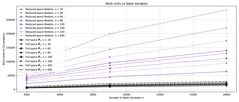
Figure 9: Scaling of work required to converge with control variables between reduced and full-space approaches.

Figure 10: Scaling of work required to converge with state variables between reduced and full-space approaches.

9 Conclusions

The necessary ingredients to implement the full-space LNKS approach within an ASO framework have been laid out, and a cost analysis of the various derivative operators is presented. A re-derivation of the $\mathbf{P}_{2}$ and $\mathbf{P}_{4}$ preconditioners of [18] yielded new preconditioners that differ from the original. However, it is analytically and numerically shown that the eigenvalue spectra are the same for the corrected preconditioned systems.

The full-and reduced-space approaches have been applied and compared on a benchmark aerodynamic problem. A dimensional analysis shows that the full-space approach with $\tilde{\mathbf{P}}_{2}$ preconditioning is the most effective method. However, its scaling will largely depend on the development of reduced-Hessian preconditioners and flow Jacobian preconditioners. Future work should aim to achieve control-independent convergence through the development of reduced-Hessian preconditioners, such as approximating the initial BFGS Hessian [12].

While the cost analysis in the present work reflects our implementation, further savings through sum factorization, collocation, and other code optimizations will affect the work ratios and is subject to further investigation. Additional work reduction within each design cycle can be achieved through inexact solves as proposed by [19] for the full-space approach, [17] for the reduced-space Newton approach, and [8] for the reduced-space quasi-Newton approach.

Appendix A Preconditioned system corrections

The purpose of this appendix is to correct the derivation from Biros and Ghattas’ preconditioned system [18]. Notation from Sec. 2 and 3 is used in the following appendix. Additionally, we will be using the following notation to simplify and shorten the derivation

$$\mathcal{L}_{yy} =\mathcal{L}_{\mathbf{u}{\boldsymbol{\alpha}}}-\mathcal{L}_{\mathbf{u}\mathbf{u}}{\boldsymbol{\mathcal{R}}}_{\mathbf{u}}^{-1}{\boldsymbol{\mathcal{R}}}_{{\boldsymbol{\alpha}}},$$ (67)

$$\mathcal{L}_{yy}^{T} =\mathcal{L}_{{\boldsymbol{\alpha}}\mathbf{u}}-{\boldsymbol{\mathcal{R}}}_{{\boldsymbol{\alpha}}}^{T}{\boldsymbol{\mathcal{R}}}_{\mathbf{u}}^{-T}\mathcal{L}_{\mathbf{u}\mathbf{u}}.$$ (68)

$$\mathcal{L}_{zz} ={\boldsymbol{\mathcal{R}}}_{{\boldsymbol{\alpha}}}^{T}{\boldsymbol{\mathcal{R}}}_{\mathbf{u}}^{-T}\mathcal{L}_{\mathbf{u}\mathbf{u}}{\boldsymbol{\mathcal{R}}}_{\mathbf{u}}^{-1}{\boldsymbol{\mathcal{R}}}_{{\boldsymbol{\alpha}}}-{\boldsymbol{\mathcal{R}}}_{{\boldsymbol{\alpha}}}^{T}{\boldsymbol{\mathcal{R}}}_{\mathbf{u}}^{-T}\mathcal{L}_{\mathbf{u}{\boldsymbol{\alpha}}}-\mathcal{L}_{{\boldsymbol{\alpha}}\mathbf{u}}{\boldsymbol{\mathcal{R}}}_{\mathbf{u}}^{-1}{\boldsymbol{\mathcal{R}}}_{{\boldsymbol{\alpha}}}+\mathcal{L}_{{\boldsymbol{\alpha}}{\boldsymbol{\alpha}}}$$ (69)

$$=-{\boldsymbol{\mathcal{R}}}_{{\boldsymbol{\alpha}}}^{T}{\boldsymbol{\mathcal{R}}}_{\mathbf{u}}^{-T}\mathcal{L}_{yy}-\mathcal{L}_{{\boldsymbol{\alpha}}\mathbf{u}}{\boldsymbol{\mathcal{R}}}_{\mathbf{u}}^{-1}{\boldsymbol{\mathcal{R}}}_{{\boldsymbol{\alpha}}}+\mathcal{L}_{{\boldsymbol{\alpha}}{\boldsymbol{\alpha}}}$$ (70)

$$=-\mathcal{L}_{yy}^{T}{\boldsymbol{\mathcal{R}}}_{\mathbf{u}}^{-1}{\boldsymbol{\mathcal{R}}}_{{\boldsymbol{\alpha}}}-{\boldsymbol{\mathcal{R}}}_{{\boldsymbol{\alpha}}}^{T}{\boldsymbol{\mathcal{R}}}_{\mathbf{u}}^{-T}\mathcal{L}_{\mathbf{u}{\boldsymbol{\alpha}}}+\mathcal{L}_{{\boldsymbol{\alpha}}{\boldsymbol{\alpha}}}.$$ (71)

When $\mathbf{P}_{4}^{-1}$ is applied to the KKT matrix $\boldsymbol{\mathcal{K}}$, we obtain

$$\begin{split}\mathbf{P}_{4}^{-1}\boldsymbol{\mathcal{K}}=\begin{bmatrix}\mathbf{I}_{\mathbf{u}}&{\boldsymbol{\mathcal{R}}}_{\mathbf{u}}^{-1}{\boldsymbol{\mathcal{R}}}_{{\boldsymbol{\alpha}}}\left(\mathbf{I}_{{\boldsymbol{\alpha}}}-\mathbf{B}_{z}^{-1}\mathcal{L}_{zz}\right)&\mathbf{0}\\ \mathbf{0}&\mathbf{B}_{z}^{-1}\mathcal{L}_{zz}&\mathbf{0}\\ \mathbf{0}&{\boldsymbol{\mathcal{R}}}_{\mathbf{u}}^{-T}\mathcal{L}_{yy}\left(\mathbf{I}_{{\boldsymbol{\alpha}}}-\mathbf{B}_{z}^{-1}\mathcal{L}_{zz}\right)&\mathbf{I}_{\mathbf{u}}\end{bmatrix}\end{split},$$ (72)

which differs from the original derivation in [18] that states

$$\begin{split}\left(\mathbf{P}_{4}^{-1}\boldsymbol{\mathcal{K}}\right)_{\text{BG}}=\begin{bmatrix}\mathbf{I}_{\mathbf{u}}&\mathbf{0}&\mathbf{0}\\ \mathbf{0}&\mathbf{B}_{z}^{-1}\mathcal{L}_{zz}&\mathbf{0}\\ \mathbf{0}&\mathbf{0}&\mathbf{I}_{\mathbf{u}}\end{bmatrix}\end{split}.$$ (73)

Furthermore, when $\mathbf{P}_{2}^{-1}$ applied to the KKT matrix $\boldsymbol{\mathcal{K}}$, we obtain

$$\begin{split}\mathbf{P}_{2}^{-1}\boldsymbol{\mathcal{K}}=\begin{bmatrix}\mathbf{I}_{\mathbf{u}}-{\boldsymbol{\mathcal{R}}}_{\mathbf{u}}^{-1}{\boldsymbol{\mathcal{R}}}_{{\boldsymbol{\alpha}}}\mathbf{B}_{z}^{-1}\mathcal{L}_{yy}^{T}&{\boldsymbol{\mathcal{R}}}_{\mathbf{u}}^{-1}{\boldsymbol{\mathcal{R}}}_{{\boldsymbol{\alpha}}}-{\boldsymbol{\mathcal{R}}}_{\mathbf{u}}^{-1}{\boldsymbol{\mathcal{R}}}_{{\boldsymbol{\alpha}}}\mathbf{B}_{z}^{-1}\left(\mathcal{L}_{zz}-\mathcal{L}_{yy}^{T}{\boldsymbol{\mathcal{R}}}_{\mathbf{u}}^{-1}{\boldsymbol{\mathcal{R}}}_{{\boldsymbol{\alpha}}}\right)&\mathbf{0}\\ \mathbf{B}_{z}^{-1}\mathcal{L}_{yy}^{T}&\mathbf{B}_{z}^{-1}\left(\mathcal{L}_{zz}+\mathcal{L}_{yy}^{T}{\boldsymbol{\mathcal{R}}}_{\mathbf{u}}^{-1}{\boldsymbol{\mathcal{R}}}_{{\boldsymbol{\alpha}}}\right)&\mathbf{0}\\ {\boldsymbol{\mathcal{R}}}_{\mathbf{u}}^{-T}\mathcal{L}_{\mathbf{u}\mathbf{u}}&{\boldsymbol{\mathcal{R}}}_{\mathbf{u}}^{-T}\mathcal{L}_{\mathbf{u}{\boldsymbol{\alpha}}}&\mathbf{I}_{\mathbf{u}}\end{bmatrix}\end{split},$$ (74)

which differs from the previously [18] derived

$$\left(\mathbf{P}_{2}^{-1}\boldsymbol{\mathcal{K}}\right)_{\text{BG}}=\begin{bmatrix}\mathbf{I}_{\mathbf{u}}&\mathbf{0}&\mathbf{0}\\ \mathcal{L}_{yy}^{T}{\boldsymbol{\mathcal{R}}}_{\mathbf{u}}^{-1}&\mathcal{L}_{zz}\mathbf{B}_{z}^{-1}&\mathbf{0}\\ \mathcal{L}_{\mathbf{u}\mathbf{u}}{\boldsymbol{\mathcal{R}}}_{\mathbf{u}}^{-1}&\mathcal{L}_{yy}\mathbf{B}_{z}^{-1}&\mathbf{I}_{\mathbf{u}}\end{bmatrix}.$$ (75)

Both of those results have been verified numerically and algebraically in C.

Furthermore, the eigenvalue spectrum of the amended preconditioned system are the same as the previously defined ones

$$\mathcal{E}\left(\mathbf{P}^{-1}_{4}\boldsymbol{\mathcal{K}}\right)=\mathcal{E}\left(\left(\mathbf{P}_{4}^{-1}\boldsymbol{\mathcal{K}}\right)_{\text{BG}}\right)=\left\{\left\{\mathcal{E}(\mathbf{B}_{z}^{-1}\mathcal{L}_{zz})\right\},\left\{\mathbf{\mathbf{I}_{s}}\right\},\left\{\mathbf{\mathbf{I}_{s}}\right\}\right\}.$$ (76)

$$\mathcal{E}\left(\mathbf{P}^{-1}_{2}\boldsymbol{\mathcal{K}}\right)=\mathcal{E}\left(\left(\mathbf{P}_{2}^{-1}\boldsymbol{\mathcal{K}}\right)_{\text{BG}}\right)=\left\{\left\{\mathcal{E}(\mathbf{B}_{z}^{-1}\mathcal{L}_{zz})\right\},\left\{\mathbf{\mathbf{I}_{s}}\right\},\left\{\mathbf{\mathbf{I}_{s}}\right\}\right\}.$$ (77)

The eigenvalues have been verified numerically and algebraically in B, which means the results from [18] still hold true.

Appendix B Preconditioned system eigenvalues

To obtain the eigenvalues of the preconditioned system $\mathbf{P}^{-1}_{4}\boldsymbol{\mathcal{K}}$, we need to find the roots of $\det\left(\mathbf{P}^{-1}_{4}\boldsymbol{\mathcal{K}}-\lambda\mathbf{I}\right)=0$

$$\begin{split}\det\left(\mathbf{P}^{-1}_{4}\boldsymbol{\mathcal{K}}-\lambda\mathbf{I}\right)&=\det\left(\begin{bmatrix}\mathbf{I}_{\mathbf{u}}-\lambda\mathbf{I}_{\mathbf{u}}&{\boldsymbol{\mathcal{R}}}_{\mathbf{u}}^{-1}{\boldsymbol{\mathcal{R}}}_{{\boldsymbol{\alpha}}}\left(\mathbf{I}_{{\boldsymbol{\alpha}}}-\mathbf{B}_{z}^{-1}\mathcal{L}_{zz}\right)&\mathbf{0}\\ \mathbf{0}&\mathbf{B}_{z}^{-1}\mathcal{L}_{zz}-\lambda\mathbf{I}_{{\boldsymbol{\alpha}}}&\mathbf{0}\\ \mathbf{0}&{\boldsymbol{\mathcal{R}}}_{\mathbf{u}}^{-T}\mathcal{L}_{yy}\left(\mathbf{I}_{{\boldsymbol{\alpha}}}-\mathbf{B}_{z}^{-1}\mathcal{L}_{zz}\right)&\mathbf{I}_{\mathbf{u}}-\lambda\mathbf{I}_{\mathbf{u}}\end{bmatrix}\right)\\ &=\det\left(\begin{bmatrix}\mathbf{M}&\mathbf{0}\\ \mathbf{N}&\mathbf{I}_{\mathbf{u}}-\lambda\mathbf{I}_{\mathbf{u}}\end{bmatrix}\right),\end{split}$$ (78)

where

$$\mathbf{M}=\begin{bmatrix}\mathbf{I}_{\mathbf{u}}-\lambda\mathbf{I}_{\mathbf{u}}&{\boldsymbol{\mathcal{R}}}_{\mathbf{u}}^{-1}{\boldsymbol{\mathcal{R}}}_{{\boldsymbol{\alpha}}}\left(\mathbf{I}_{{\boldsymbol{\alpha}}}-\mathbf{B}_{z}^{-1}\mathcal{L}_{zz}\right)\\ \mathbf{0}&\mathbf{B}_{z}^{-1}\mathcal{L}_{zz}-\lambda\mathbf{I}_{{\boldsymbol{\alpha}}}\\ \end{bmatrix}\quad\text{ and }\quad\mathbf{N}=\begin{bmatrix}\mathbf{0}&{\boldsymbol{\mathcal{R}}}_{\mathbf{u}}^{-T}\mathcal{L}_{yy}\left(\mathbf{I}_{{\boldsymbol{\alpha}}}-\mathbf{B}_{z}^{-1}\mathcal{L}_{zz}\right)\end{bmatrix}.$$ (79)

Therefore, the eigenvalues of $\mathbf{P}^{-1}_{4}\boldsymbol{\mathcal{K}}$ satisfy the roots of

$$\begin{split}\det\left(\mathbf{P}^{-1}_{4}\boldsymbol{\mathcal{K}}-\lambda\mathbf{I}\right)&=\det\left(\mathbf{M}\right)\det\left(\mathbf{I}_{\mathbf{u}}-\lambda\mathbf{I}_{\mathbf{u}}\right)\\ &=\det\left(\mathbf{I}_{\mathbf{u}}-\lambda\mathbf{I}_{\mathbf{u}}\right)\det\left(\mathbf{B}_{z}^{-1}\mathcal{L}_{zz}-\lambda\mathbf{I}_{{\boldsymbol{\alpha}}}\right)\det\left(\mathbf{I}_{\mathbf{u}}-\lambda\mathbf{I}_{\mathbf{u}}\right)=0.\end{split}$$ (80)

The preconditioned system $\mathbf{P}^{-1}_{4}\boldsymbol{\mathcal{K}}$ therefore has the root 1 with a multiplicity of $2m$, and the other roots corresponding to the eigenvalues of $\mathbf{B}_{z}^{-1}\mathcal{L}_{zz}$.

We repeat the process for the eigenvalues of $\mathbf{P}_{2}^{-1}\boldsymbol{\mathcal{K}}$

$$\begin{split}&\det\left(\mathbf{P}_{2}^{-1}\boldsymbol{\mathcal{K}}-\lambda\mathbf{I}\right)\\ &\quad=\det\left(\begin{bmatrix}\left(\begin{aligned} &\mathbf{I}_{\mathbf{u}}-\lambda\mathbf{I}_{\mathbf{u}}\\ &\quad-{\boldsymbol{\mathcal{R}}}_{\mathbf{u}}^{-1}{\boldsymbol{\mathcal{R}}}_{{\boldsymbol{\alpha}}}\mathbf{B}_{z}^{-1}\mathcal{L}_{yy}^{T}\end{aligned}\right)&\left(\begin{aligned} &{\boldsymbol{\mathcal{R}}}_{\mathbf{u}}^{-1}{\boldsymbol{\mathcal{R}}}_{{\boldsymbol{\alpha}}}\\ &\quad-{\boldsymbol{\mathcal{R}}}_{\mathbf{u}}^{-1}{\boldsymbol{\mathcal{R}}}_{{\boldsymbol{\alpha}}}\mathbf{B}_{z}^{-1}\left(\mathcal{L}_{zz}-\mathcal{L}_{yy}^{T}{\boldsymbol{\mathcal{R}}}_{\mathbf{u}}^{-1}{\boldsymbol{\mathcal{R}}}_{{\boldsymbol{\alpha}}}\right)\end{aligned}\right)&\mathbf{0}\\ \mathbf{B}_{z}^{-1}\mathcal{L}_{yy}^{T}&\mathbf{B}_{z}^{-1}\left(\mathcal{L}_{zz}+\mathcal{L}_{yy}^{T}{\boldsymbol{\mathcal{R}}}_{\mathbf{u}}^{-1}{\boldsymbol{\mathcal{R}}}_{{\boldsymbol{\alpha}}}\right)-\lambda\mathbf{I}_{{\boldsymbol{\alpha}}}&\mathbf{0}\\ {\boldsymbol{\mathcal{R}}}_{\mathbf{u}}^{-T}\mathcal{L}_{\mathbf{u}\mathbf{u}}&{\boldsymbol{\mathcal{R}}}_{\mathbf{u}}^{-T}\mathcal{L}_{\mathbf{u}{\boldsymbol{\alpha}}}&\mathbf{I}_{\mathbf{u}}-\lambda\mathbf{I}_{\mathbf{u}}\end{bmatrix}\right)\\ &\quad=\det\left(\begin{bmatrix}\mathbf{I}_{\mathbf{u}}&-{\boldsymbol{\mathcal{R}}}_{\mathbf{u}}^{-1}{\boldsymbol{\mathcal{R}}}_{{\boldsymbol{\alpha}}}&\mathbf{0}\\ \mathbf{0}&\mathbf{I}_{{\boldsymbol{\alpha}}}&\mathbf{0}\\ \mathbf{0}&\mathbf{0}&\mathbf{I}_{\mathbf{u}}\end{bmatrix}\begin{bmatrix}\mathbf{I}_{\mathbf{u}}-\lambda\mathbf{I}_{\mathbf{u}}&{\boldsymbol{\mathcal{R}}}_{\mathbf{u}}^{-1}{\boldsymbol{\mathcal{R}}}_{{\boldsymbol{\alpha}}}\left(\mathbf{I}_{{\boldsymbol{\alpha}}}-\lambda\mathbf{I}_{{\boldsymbol{\alpha}}}\right)&\mathbf{0}\\ \mathbf{B}_{z}^{-1}\mathcal{L}_{yy}^{T}&\mathbf{B}_{z}^{-1}\left(\mathcal{L}_{zz}+\mathcal{L}_{yy}^{T}{\boldsymbol{\mathcal{R}}}_{\mathbf{u}}^{-1}{\boldsymbol{\mathcal{R}}}_{{\boldsymbol{\alpha}}}\right)-\lambda\mathbf{I}_{{\boldsymbol{\alpha}}}&\mathbf{0}\\ {\boldsymbol{\mathcal{R}}}_{\mathbf{u}}^{-T}\mathcal{L}_{\mathbf{u}\mathbf{u}}&{\boldsymbol{\mathcal{R}}}_{\mathbf{u}}^{-T}\mathcal{L}_{\mathbf{u}{\boldsymbol{\alpha}}}&\mathbf{I}_{\mathbf{u}}-\lambda\mathbf{I}_{\mathbf{u}}\end{bmatrix}\right)\\ &\quad=\det\left(\begin{bmatrix}\mathbf{I}_{\mathbf{u}}&-{\boldsymbol{\mathcal{R}}}_{\mathbf{u}}^{-1}{\boldsymbol{\mathcal{R}}}_{{\boldsymbol{\alpha}}}&\mathbf{0}\\ \mathbf{0}&\mathbf{I}_{{\boldsymbol{\alpha}}}&\mathbf{0}\\ \mathbf{0}&\mathbf{0}&\mathbf{I}_{\mathbf{u}}\end{bmatrix}\right)\det\left(\begin{bmatrix}\mathbf{R}&\mathbf{0}\\ \mathbf{S}&\mathbf{I}_{\mathbf{u}}-\lambda\mathbf{I}_{\mathbf{u}}\end{bmatrix}\right).\end{split}$$ (81)

Let,

$$\mathbf{R}=\begin{bmatrix}\mathbf{I}_{\mathbf{u}}-\lambda\mathbf{I}_{\mathbf{u}}&{\boldsymbol{\mathcal{R}}}_{\mathbf{u}}^{-1}{\boldsymbol{\mathcal{R}}}_{{\boldsymbol{\alpha}}}\left(\mathbf{I}_{{\boldsymbol{\alpha}}}-\lambda\mathbf{I}_{{\boldsymbol{\alpha}}}\right)\\ \mathbf{B}_{z}^{-1}\mathcal{L}_{yy}^{T}&\mathbf{B}_{z}^{-1}\left(\mathcal{L}_{zz}+\mathcal{L}_{yy}^{T}{\boldsymbol{\mathcal{R}}}_{\mathbf{u}}^{-1}{\boldsymbol{\mathcal{R}}}_{{\boldsymbol{\alpha}}}\right)-\lambda\mathbf{I}_{{\boldsymbol{\alpha}}}\end{bmatrix}\quad\text{ and }\quad\mathbf{S}=\begin{bmatrix}{\boldsymbol{\mathcal{R}}}_{\mathbf{u}}^{-T}\mathcal{L}_{\mathbf{u}\mathbf{u}}&{\boldsymbol{\mathcal{R}}}_{\mathbf{u}}^{-T}\mathcal{L}_{\mathbf{u}{\boldsymbol{\alpha}}}\end{bmatrix}.$$ (82)

The eigenvalues of $\mathbf{P}_{2}^{-1}\boldsymbol{\mathcal{K}}$ are the roots of

$$\begin{split}\det\left(\mathbf{P}_{2}^{-1}\boldsymbol{\mathcal{K}}-\lambda\mathbf{I}\right)&=\det\left(\mathbf{I}_{\mathbf{u}}\right)\det\left(\mathbf{I}_{{\boldsymbol{\alpha}}}\right)\det\left(\mathbf{I}_{\mathbf{u}}\right)\det\left(\mathbf{R}\right)\det\left(\mathbf{I}_{\mathbf{u}}-\lambda\mathbf{I}_{\mathbf{u}}\right)=0\end{split}.$$ (83)

For a matrix

$$M=\begin{bmatrix}A&B\\ C&D\end{bmatrix},$$ (84)

where $A$ is invertible, the determinant of $M$ is given by

$$\det\left(M\right)=\det\left(A\right)\det\left(D-CA^{-1}B\right)$$ (85)

Note that if $\lambda=1$, $\left(\mathbf{I}_{\mathbf{u}}-\lambda\mathbf{I}_{\mathbf{u}}\right)$ is not invertible, but $\det\left(\mathbf{R}\right)=0$ nonetheless. If $\lambda\neq 1$, we can use Eq. (85) to obtain

$$\begin{split}\det\left(\mathbf{R}\right)&=\det\left(\mathbf{I}_{\mathbf{u}}-\lambda\mathbf{I}_{\mathbf{u}}\right)\det\left(\mathbf{B}_{z}^{-1}\left(\mathcal{L}_{zz}+\mathcal{L}_{yy}^{T}{\boldsymbol{\mathcal{R}}}_{\mathbf{u}}^{-1}{\boldsymbol{\mathcal{R}}}_{{\boldsymbol{\alpha}}}\right)\right.\\ &\quad\quad\quad\left.-\lambda\mathbf{I}_{{\boldsymbol{\alpha}}}-\left(\mathbf{B}_{z}^{-1}\mathcal{L}_{yy}^{T}\right)\left(\mathbf{I}_{\mathbf{u}}-\lambda\mathbf{I}_{\mathbf{u}}\right)^{-1}\left({\boldsymbol{\mathcal{R}}}_{\mathbf{u}}^{-1}{\boldsymbol{\mathcal{R}}}_{{\boldsymbol{\alpha}}}\left(\mathbf{I}_{{\boldsymbol{\alpha}}}-\lambda\mathbf{I}_{{\boldsymbol{\alpha}}}\right)\right)\right)\\ &=\det\left(\mathbf{I}_{\mathbf{u}}-\lambda\mathbf{I}_{\mathbf{u}}\right)\det\left(\mathbf{B}_{z}^{-1}\mathcal{L}_{zz}+\mathbf{B}_{z}^{-1}\mathcal{L}_{yy}^{T}{\boldsymbol{\mathcal{R}}}_{\mathbf{u}}^{-1}{\boldsymbol{\mathcal{R}}}_{{\boldsymbol{\alpha}}}\right.\\ &\quad\quad\quad\left.-\lambda\mathbf{I}_{{\boldsymbol{\alpha}}}-\left(\mathbf{B}_{z}^{-1}\mathcal{L}_{yy}^{T}\right)\left({\boldsymbol{\mathcal{R}}}_{\mathbf{u}}^{-1}{\boldsymbol{\mathcal{R}}}_{{\boldsymbol{\alpha}}}\right)\right)\\ &=\det\left(\mathbf{I}_{\mathbf{u}}-\lambda\mathbf{I}_{\mathbf{u}}\right)\det\left(\mathbf{B}_{z}^{-1}\mathcal{L}_{zz}-\lambda\mathbf{I}_{{\boldsymbol{\alpha}}}\right).\end{split}$$ (86)

Therefore,

$$\begin{split}\det\left(\mathbf{P}_{2}^{-1}\boldsymbol{\mathcal{K}}-\lambda\mathbf{I}\right)&=\det\left(\mathbf{R}\right)\det\left(\mathbf{I}_{\mathbf{u}}-\lambda\mathbf{I}_{\mathbf{u}}\right)\\ &=\det\left(\mathbf{I}_{\mathbf{u}}-\lambda\mathbf{I}_{\mathbf{u}}\right)\det\left(\mathbf{B}_{z}^{-1}\mathcal{L}_{zz}-\lambda\mathbf{I}_{{\boldsymbol{\alpha}}}\right)\det\left(\mathbf{I}_{\mathbf{u}}-\lambda\mathbf{I}_{\mathbf{u}}\right)=0\end{split}$$ (87)

results in the same roots as the previous preconditioned system.

Appendix C Preconditioned system derivation

To derive the inverses, we start by checking what the $\mathbf{P}_{4}$ operator can be represented as

$$\mathbf{P}_{4} =\boldsymbol{\mathcal{K}}_{1}\boldsymbol{\mathcal{K}}_{2} =\begin{bmatrix}\mathcal{L}_{\mathbf{u}\mathbf{u}}{\boldsymbol{\mathcal{R}}}_{\mathbf{u}}^{-1}&\mathbf{0}&\mathbf{I}\\ \mathcal{L}_{{\boldsymbol{\alpha}}\mathbf{u}}{\boldsymbol{\mathcal{R}}}_{\mathbf{u}}^{-1}&\mathbf{I}&{\boldsymbol{\mathcal{R}}}_{{\boldsymbol{\alpha}}}^{T}{\boldsymbol{\mathcal{R}}}_{\mathbf{u}}^{-T}\\ \mathbf{I}&\mathbf{0}&\mathbf{0}\end{bmatrix}\begin{bmatrix}{\boldsymbol{\mathcal{R}}}_{\mathbf{u}}&{\boldsymbol{\mathcal{R}}}_{{\boldsymbol{\alpha}}}&\mathbf{0}\\ \mathbf{0}&\mathbf{B}_{z}&\mathbf{0}\\ \mathbf{0}&\left(\mathcal{L}_{\mathbf{u}{\boldsymbol{\alpha}}}-\mathcal{L}_{\mathbf{u}\mathbf{u}}{\boldsymbol{\mathcal{R}}}_{\mathbf{u}}^{-1}{\boldsymbol{\mathcal{R}}}_{{\boldsymbol{\alpha}}}\right)&{\boldsymbol{\mathcal{R}}}_{\mathbf{u}}^{T}\end{bmatrix}$$ (88)

$$=\begin{bmatrix}\mathcal{L}_{\mathbf{u}\mathbf{u}}&\mathcal{L}_{\mathbf{u}{\boldsymbol{\alpha}}}&{\boldsymbol{\mathcal{R}}}_{\mathbf{u}}^{T}\\ \mathcal{L}_{{\boldsymbol{\alpha}}\mathbf{u}}&\mathcal{L}_{{\boldsymbol{\alpha}}\mathbf{u}}{\boldsymbol{\mathcal{R}}}_{\mathbf{u}}^{-1}{\boldsymbol{\mathcal{R}}}_{{\boldsymbol{\alpha}}}+\mathbf{B}_{z}+{\boldsymbol{\mathcal{R}}}_{{\boldsymbol{\alpha}}}^{T}{\boldsymbol{\mathcal{R}}}_{\mathbf{u}}^{-T}\left(\mathcal{L}_{\mathbf{u}{\boldsymbol{\alpha}}}-\mathcal{L}_{\mathbf{u}\mathbf{u}}{\boldsymbol{\mathcal{R}}}_{\mathbf{u}}^{-1}{\boldsymbol{\mathcal{R}}}_{{\boldsymbol{\alpha}}}\right)&{\boldsymbol{\mathcal{R}}}_{{\boldsymbol{\alpha}}}^{T}\\ {\boldsymbol{\mathcal{R}}}_{\mathbf{u}}&{\boldsymbol{\mathcal{R}}}_{{\boldsymbol{\alpha}}}&\mathbf{0}\end{bmatrix}$$

$$=\begin{bmatrix}\mathcal{L}_{\mathbf{u}\mathbf{u}}&\mathcal{L}_{\mathbf{u}{\boldsymbol{\alpha}}}&{\boldsymbol{\mathcal{R}}}_{\mathbf{u}}^{T}\\ \mathcal{L}_{{\boldsymbol{\alpha}}\mathbf{u}}&\mathbf{B}_{z}-\mathcal{L}_{zz}+\mathcal{L}_{{\boldsymbol{\alpha}}{\boldsymbol{\alpha}}}&{\boldsymbol{\mathcal{R}}}_{{\boldsymbol{\alpha}}}^{T}\\ {\boldsymbol{\mathcal{R}}}_{\mathbf{u}}&{\boldsymbol{\mathcal{R}}}_{{\boldsymbol{\alpha}}}&\mathbf{0}\end{bmatrix}.$$

Therefore, if $\mathbf{B}_{z}=\mathcal{L}_{zz}$, we recover the KKT matrix as expected.

Let’s find $\boldsymbol{\mathcal{K}}_{1}^{-1}$

$$\begin{bmatrix}\mathcal{L}_{\mathbf{u}\mathbf{u}}{\boldsymbol{\mathcal{R}}}_{\mathbf{u}}^{-1}&\mathbf{0}&\mathbf{I}\\ \mathcal{L}_{{\boldsymbol{\alpha}}\mathbf{u}}{\boldsymbol{\mathcal{R}}}_{\mathbf{u}}^{-1}&\mathbf{I}&{\boldsymbol{\mathcal{R}}}_{{\boldsymbol{\alpha}}}^{T}{\boldsymbol{\mathcal{R}}}_{\mathbf{u}}^{-T}\\ \mathbf{I}&\mathbf{0}&\mathbf{0}\end{bmatrix}\begin{bmatrix}\left(\boldsymbol{\mathcal{K}}_{1}^{-1}\right)_{11}&\left(\boldsymbol{\mathcal{K}}_{1}^{-1}\right)_{12}&\left(\boldsymbol{\mathcal{K}}_{1}^{-1}\right)_{13}\\ \left(\boldsymbol{\mathcal{K}}_{1}^{-1}\right)_{21}&\left(\boldsymbol{\mathcal{K}}_{1}^{-1}\right)_{22}&\left(\boldsymbol{\mathcal{K}}_{1}^{-1}\right)_{23}\\ \left(\boldsymbol{\mathcal{K}}_{1}^{-1}\right)_{31}&\left(\boldsymbol{\mathcal{K}}_{1}^{-1}\right)_{32}&\left(\boldsymbol{\mathcal{K}}_{1}^{-1}\right)_{33}\end{bmatrix}=\begin{bmatrix}\mathbf{I}_{\mathbf{u}}&\mathbf{0}&\mathbf{0}\\ \mathbf{0}&\mathbf{I}_{{\boldsymbol{\alpha}}}&\mathbf{0}\\ \mathbf{0}&\mathbf{0}&\mathbf{I}_{\mathbf{u}}\end{bmatrix}.$$ (89)

The first column forms

$${\mathcal{L}_{\mathbf{u}\mathbf{u}}{\boldsymbol{\mathcal{R}}}_{\mathbf{u}}^{-1}\left(\boldsymbol{\mathcal{K}}_{1}^{-1}\right)_{11}} +{\mathbf{I}_{\mathbf{u}}\left(\boldsymbol{\mathcal{K}}_{1}^{-1}\right)_{31}} = \mathbf{I}_{\mathbf{u}},$$ (90)

$${\mathcal{L}_{{\boldsymbol{\alpha}}\mathbf{u}}{\boldsymbol{\mathcal{R}}}_{\mathbf{u}}^{-1}\left(\boldsymbol{\mathcal{K}}_{1}^{-1}\right)_{11}} +{\mathbf{I}_{{\boldsymbol{\alpha}}}\left(\boldsymbol{\mathcal{K}}_{1}^{-1}\right)_{21}} +{{\boldsymbol{\mathcal{R}}}_{{\boldsymbol{\alpha}}}^{T}{\boldsymbol{\mathcal{R}}}_{\mathbf{u}}^{-T}\left(\boldsymbol{\mathcal{K}}_{1}^{-1}\right)_{31}} = \mathbf{0},$$

$${\mathbf{I}_{\mathbf{u}}\left(\boldsymbol{\mathcal{K}}_{1}^{-1}\right)_{11}} = \mathbf{0},$$

which gives

$$\left(\boldsymbol{\mathcal{K}}_{1}^{-1}\right)_{11} =\mathbf{0},$$ (91)

$$\left(\boldsymbol{\mathcal{K}}_{1}^{-1}\right)_{31} =\left(\mathbf{I}_{\mathbf{u}}-\mathcal{L}_{\mathbf{u}\mathbf{u}}{\boldsymbol{\mathcal{R}}}_{\mathbf{u}}^{-1}\mathbf{T}_{11}\right) =\mathbf{I}_{\mathbf{u}},$$

$$\left(\boldsymbol{\mathcal{K}}_{1}^{-1}\right)_{21} =-\mathcal{L}_{{\boldsymbol{\alpha}}\mathbf{u}}{\boldsymbol{\mathcal{R}}}_{\mathbf{u}}^{-1}\left(\boldsymbol{\mathcal{K}}_{1}^{-1}\right)_{11}-{\boldsymbol{\mathcal{R}}}_{{\boldsymbol{\alpha}}}^{T}{\boldsymbol{\mathcal{R}}}_{\mathbf{u}}^{-T}\left(\boldsymbol{\mathcal{K}}_{1}^{-1}\right)_{31} =-{\boldsymbol{\mathcal{R}}}_{{\boldsymbol{\alpha}}}^{T}{\boldsymbol{\mathcal{R}}}_{\mathbf{u}}^{-T}.$$

The second column forms

$${\mathcal{L}_{\mathbf{u}\mathbf{u}}{\boldsymbol{\mathcal{R}}}_{\mathbf{u}}^{-1}\left(\boldsymbol{\mathcal{K}}_{1}^{-1}\right)_{12}} +{\mathbf{I}_{\mathbf{u}}\left(\boldsymbol{\mathcal{K}}_{1}^{-1}\right)_{32}} = \mathbf{0},$$ (92)

$${\mathcal{L}_{{\boldsymbol{\alpha}}\mathbf{u}}{\boldsymbol{\mathcal{R}}}_{\mathbf{u}}^{-1}\left(\boldsymbol{\mathcal{K}}_{1}^{-1}\right)_{12}} +{\mathbf{I}_{{\boldsymbol{\alpha}}}\left(\boldsymbol{\mathcal{K}}_{1}^{-1}\right)_{22}} +{{\boldsymbol{\mathcal{R}}}_{{\boldsymbol{\alpha}}}^{T}{\boldsymbol{\mathcal{R}}}_{\mathbf{u}}^{-T}\left(\boldsymbol{\mathcal{K}}_{1}^{-1}\right)_{32}} = \mathbf{I}_{{\boldsymbol{\alpha}}},$$

$${\mathbf{I}_{\mathbf{u}}\left(\boldsymbol{\mathcal{K}}_{1}^{-1}\right)_{12}} = \mathbf{0},$$

which gives

$$\left(\boldsymbol{\mathcal{K}}_{1}^{-1}\right)_{12} =\mathbf{0},$$ (93)

$$\left(\boldsymbol{\mathcal{K}}_{1}^{-1}\right)_{32} =-\mathcal{L}_{\mathbf{u}\mathbf{u}}{\boldsymbol{\mathcal{R}}}_{\mathbf{u}}^{-1}\left(\boldsymbol{\mathcal{K}}_{1}^{-1}\right)_{12} =\mathbf{0},$$

$$\left(\boldsymbol{\mathcal{K}}_{1}^{-1}\right)_{22} =\mathbf{I}_{{\boldsymbol{\alpha}}}-\mathcal{L}_{{\boldsymbol{\alpha}}\mathbf{u}}{\boldsymbol{\mathcal{R}}}_{\mathbf{u}}^{-1}\left(\boldsymbol{\mathcal{K}}_{1}^{-1}\right)_{12}-{\boldsymbol{\mathcal{R}}}_{{\boldsymbol{\alpha}}}^{T}{\boldsymbol{\mathcal{R}}}_{\mathbf{u}}^{-T}\left(\boldsymbol{\mathcal{K}}_{1}^{-1}\right)_{32} =\mathbf{I}_{{\boldsymbol{\alpha}}}.$$

The third column forms

$${\mathcal{L}_{\mathbf{u}\mathbf{u}}{\boldsymbol{\mathcal{R}}}_{\mathbf{u}}^{-1}\left(\boldsymbol{\mathcal{K}}_{1}^{-1}\right)_{13}} +{\mathbf{I}_{\mathbf{u}}\left(\boldsymbol{\mathcal{K}}_{1}^{-1}\right)_{33}} = \mathbf{0},$$ (94)

$${\mathcal{L}_{{\boldsymbol{\alpha}}\mathbf{u}}{\boldsymbol{\mathcal{R}}}_{\mathbf{u}}^{-1}\left(\boldsymbol{\mathcal{K}}_{1}^{-1}\right)_{13}} +{\mathbf{I}_{{\boldsymbol{\alpha}}}\left(\boldsymbol{\mathcal{K}}_{1}^{-1}\right)_{23}} +{{\boldsymbol{\mathcal{R}}}_{{\boldsymbol{\alpha}}}^{T}{\boldsymbol{\mathcal{R}}}_{\mathbf{u}}^{-T}\left(\boldsymbol{\mathcal{K}}_{1}^{-1}\right)_{33}} = \mathbf{0},$$

$${\mathbf{I}_{\mathbf{u}}\left(\boldsymbol{\mathcal{K}}_{1}^{-1}\right)_{13}} = \mathbf{I}_{\mathbf{u}},$$

which gives

$$\left(\boldsymbol{\mathcal{K}}_{1}^{-1}\right)_{13} =\mathbf{I}_{\mathbf{u}},$$ (95)

$$\left(\boldsymbol{\mathcal{K}}_{1}^{-1}\right)_{33} =-\mathcal{L}_{\mathbf{u}\mathbf{u}}{\boldsymbol{\mathcal{R}}}_{\mathbf{u}}^{-1}\left(\boldsymbol{\mathcal{K}}_{1}^{-1}\right)_{13} =-\mathcal{L}_{\mathbf{u}\mathbf{u}}{\boldsymbol{\mathcal{R}}}_{\mathbf{u}}^{-1},$$

$$\left(\boldsymbol{\mathcal{K}}_{1}^{-1}\right)_{23} =-\mathcal{L}_{{\boldsymbol{\alpha}}\mathbf{u}}{\boldsymbol{\mathcal{R}}}_{\mathbf{u}}^{-1}\left(\boldsymbol{\mathcal{K}}_{1}^{-1}\right)_{13}-{\boldsymbol{\mathcal{R}}}_{{\boldsymbol{\alpha}}}^{T}{\boldsymbol{\mathcal{R}}}_{\mathbf{u}}^{-T}\left(\boldsymbol{\mathcal{K}}_{1}^{-1}\right)_{33}$$

$$=-\mathcal{L}_{{\boldsymbol{\alpha}}\mathbf{u}}{\boldsymbol{\mathcal{R}}}_{\mathbf{u}}^{-1}+{\boldsymbol{\mathcal{R}}}_{{\boldsymbol{\alpha}}}^{T}{\boldsymbol{\mathcal{R}}}_{\mathbf{u}}^{-T}\mathcal{L}_{\mathbf{u}\mathbf{u}}{\boldsymbol{\mathcal{R}}}_{\mathbf{u}}^{-1}=-\mathcal{L}_{yy}^{T}{\boldsymbol{\mathcal{R}}}_{\mathbf{u}}^{-1}.$$

Repeat the whole process for $\boldsymbol{\mathcal{K}}_{2}$. The first column gives

$$\left(\boldsymbol{\mathcal{K}}_{2}^{-1}\right)_{21} =\mathbf{0},$$ (96)

$$\left(\boldsymbol{\mathcal{K}}_{2}^{-1}\right)_{11} ={\boldsymbol{\mathcal{R}}}_{\mathbf{u}}^{-1}\left(\mathbf{I}_{\mathbf{u}}-{\boldsymbol{\mathcal{R}}}_{{\boldsymbol{\alpha}}}\left(\boldsymbol{\mathcal{K}}_{2}^{-1}\right)_{21}\right) ={\boldsymbol{\mathcal{R}}}_{\mathbf{u}}^{-1},$$

$$\left(\boldsymbol{\mathcal{K}}_{2}^{-1}\right)_{31} =-{\boldsymbol{\mathcal{R}}}_{\mathbf{u}}^{-T}\mathcal{L}_{yy}\left(\boldsymbol{\mathcal{K}}_{2}^{-1}\right)_{21} =\mathbf{0}.$$

The second column results in

$$\left(\boldsymbol{\mathcal{K}}_{2}^{-1}\right)_{22} =\mathbf{B}_{z}^{-1}\mathbf{I}_{{\boldsymbol{\alpha}}} =\mathbf{B}_{z}^{-1},$$ (97)

$$\left(\boldsymbol{\mathcal{K}}_{2}^{-1}\right)_{12} =-{\boldsymbol{\mathcal{R}}}_{\mathbf{u}}^{-1}{\boldsymbol{\mathcal{R}}}_{{\boldsymbol{\alpha}}}\left(\boldsymbol{\mathcal{K}}_{2}^{-1}\right)_{22} =-{\boldsymbol{\mathcal{R}}}_{\mathbf{u}}^{-1}{\boldsymbol{\mathcal{R}}}_{{\boldsymbol{\alpha}}}\mathbf{B}_{z}^{-1},$$

$$\left(\boldsymbol{\mathcal{K}}_{2}^{-1}\right)_{32} =-{\boldsymbol{\mathcal{R}}}_{\mathbf{u}}^{-T}\mathcal{L}_{yy}\left(\boldsymbol{\mathcal{K}}_{2}^{-1}\right)_{22} =-{\boldsymbol{\mathcal{R}}}_{\mathbf{u}}^{-T}\mathcal{L}_{yy}\mathbf{B}_{z}^{-1}.$$

The third column results in

$$\left(\boldsymbol{\mathcal{K}}_{2}^{-1}\right)_{23} =\mathbf{0},$$ (98)

$$\left(\boldsymbol{\mathcal{K}}_{2}^{-1}\right)_{13} =-{\boldsymbol{\mathcal{R}}}_{\mathbf{u}}^{-1}{\boldsymbol{\mathcal{R}}}_{{\boldsymbol{\alpha}}}\left(\boldsymbol{\mathcal{K}}_{2}^{-1}\right)_{23} =\mathbf{0},$$

$$\left(\boldsymbol{\mathcal{K}}_{2}^{-1}\right)_{33} ={\boldsymbol{\mathcal{R}}}_{\mathbf{u}}^{-T}\left(\mathbf{I}_{\mathbf{u}}-\mathcal{L}_{yy}\left(\boldsymbol{\mathcal{K}}_{2}^{-1}\right)_{23}\right) ={\boldsymbol{\mathcal{R}}}_{\mathbf{u}}^{-T}.$$

Finally, the inverse of $\boldsymbol{\mathcal{K}}_{1}$ is given by

$$\boldsymbol{\mathcal{K}}_{1}^{-1}=\begin{bmatrix}\mathbf{0}&\mathbf{0}&\mathbf{I}_{\mathbf{u}}\\ -{\boldsymbol{\mathcal{R}}}_{{\boldsymbol{\alpha}}}^{T}{\boldsymbol{\mathcal{R}}}_{\mathbf{u}}^{-T}&\mathbf{I}_{{\boldsymbol{\alpha}}}&-\mathcal{L}_{yy}^{T}{\boldsymbol{\mathcal{R}}}_{\mathbf{u}}^{-1}\\ \mathbf{I}_{\mathbf{u}}&\mathbf{0}&-\mathcal{L}_{\mathbf{u}\mathbf{u}}{\boldsymbol{\mathcal{R}}}_{\mathbf{u}}^{-1}\end{bmatrix},$$ (99)

and the inverse of $\boldsymbol{\mathcal{K}}_{2}$ is given by

$$\boldsymbol{\mathcal{K}}_{2}^{-1}=\begin{bmatrix}{\boldsymbol{\mathcal{R}}}_{\mathbf{u}}^{-1}&-{\boldsymbol{\mathcal{R}}}_{\mathbf{u}}^{-1}{\boldsymbol{\mathcal{R}}}_{{\boldsymbol{\alpha}}}\mathbf{B}_{z}^{-1}&\mathbf{0}\\ \mathbf{0}&\mathbf{B}_{z}^{-1}&\mathbf{0}\\ \mathbf{0}&-{\boldsymbol{\mathcal{R}}}_{\mathbf{u}}^{-T}\mathcal{L}_{yy}\mathbf{B}_{z}^{-1}&{\boldsymbol{\mathcal{R}}}_{\mathbf{u}}^{-T}\end{bmatrix}.$$ (100)

Finally, the inverse of the $\mathbf{P}_{4}$ preconditioner is given by

$$\mathbf{P}_{4}^{-1}=\left(\boldsymbol{\mathcal{K}}_{1}\boldsymbol{\mathcal{K}}_{2}\right)^{-1}=\boldsymbol{\mathcal{K}}_{2}^{-1}\boldsymbol{\mathcal{K}}_{1}^{-1}.$$ (101)

$$\begin{split}\left(\mathbf{P}_{4}^{-1}\right)_{11}&={\boldsymbol{\mathcal{R}}}_{\mathbf{u}}^{-1}{\boldsymbol{\mathcal{R}}}_{{\boldsymbol{\alpha}}}\mathbf{B}_{z}^{-1}{\boldsymbol{\mathcal{R}}}_{{\boldsymbol{\alpha}}}^{T}{\boldsymbol{\mathcal{R}}}_{\mathbf{u}}^{-T},\\ \left(\mathbf{P}_{4}^{-1}\right)_{12}&=-{\boldsymbol{\mathcal{R}}}_{\mathbf{u}}^{-1}{\boldsymbol{\mathcal{R}}}_{{\boldsymbol{\alpha}}}\mathbf{B}_{z}^{-1},\\ \left(\mathbf{P}_{4}^{-1}\right)_{13}&={\boldsymbol{\mathcal{R}}}_{\mathbf{u}}^{-1}+{\boldsymbol{\mathcal{R}}}_{\mathbf{u}}^{-1}{\boldsymbol{\mathcal{R}}}_{{\boldsymbol{\alpha}}}\mathbf{B}_{z}^{-1}\mathcal{L}_{yy}^{T}{\boldsymbol{\mathcal{R}}}_{\mathbf{u}}^{-1},\\ \left(\mathbf{P}_{4}^{-1}\right)_{21}&=-\mathbf{B}_{z}^{-1}{\boldsymbol{\mathcal{R}}}_{{\boldsymbol{\alpha}}}^{T}{\boldsymbol{\mathcal{R}}}_{\mathbf{u}}^{-T},\\ \left(\mathbf{P}_{4}^{-1}\right)_{22}&=\mathbf{B}_{z}^{-1},\\ \left(\mathbf{P}_{4}^{-1}\right)_{23}&=-\mathbf{B}_{z}^{-1}\mathcal{L}_{yy}^{T}{\boldsymbol{\mathcal{R}}}_{\mathbf{u}}^{-1},\\ \left(\mathbf{P}_{4}^{-1}\right)_{31}&={\boldsymbol{\mathcal{R}}}_{\mathbf{u}}^{-T}\mathcal{L}_{yy}\mathbf{B}_{z}^{-1}{\boldsymbol{\mathcal{R}}}_{{\boldsymbol{\alpha}}}^{T}{\boldsymbol{\mathcal{R}}}_{\mathbf{u}}^{-T}-{\boldsymbol{\mathcal{R}}}_{\mathbf{u}}^{-T},\\ \left(\mathbf{P}_{4}^{-1}\right)_{32}&=-{\boldsymbol{\mathcal{R}}}_{\mathbf{u}}^{-T}\mathcal{L}_{yy}\mathbf{B}_{z}^{-1},\\ \left(\mathbf{P}_{4}^{-1}\right)_{33}&={\boldsymbol{\mathcal{R}}}_{\mathbf{u}}^{-T}\mathcal{L}_{yy}\mathbf{B}_{z}^{-1}\mathcal{L}_{yy}^{T}{\boldsymbol{\mathcal{R}}}_{\mathbf{u}}^{-1}-{\boldsymbol{\mathcal{R}}}_{\mathbf{u}}^{-T}\mathcal{L}_{\mathbf{u}\mathbf{u}}{\boldsymbol{\mathcal{R}}}_{\mathbf{u}}^{-1}.\end{split}$$ (102)

Multiplying the inverse of the preconditioner $\mathbf{P}_{4}^{-1}$ with the KKT matrix $\boldsymbol{\mathcal{K}}$ gives the following preconditioned system

$$\mathbf{P}_{4}^{-1}\boldsymbol{\mathcal{K}}=\mathbf{C}$$ (103)

$$\mathbf{C}_{11} ={\boldsymbol{\mathcal{R}}}_{\mathbf{u}}^{-1}{\boldsymbol{\mathcal{R}}}_{{\boldsymbol{\alpha}}}\mathbf{B}_{z}^{-1}{\boldsymbol{\mathcal{R}}}_{{\boldsymbol{\alpha}}}^{T}{\boldsymbol{\mathcal{R}}}_{\mathbf{u}}^{-T}\mathcal{L}_{\mathbf{u}\mathbf{u}}-{\boldsymbol{\mathcal{R}}}_{\mathbf{u}}^{-1}{\boldsymbol{\mathcal{R}}}_{{\boldsymbol{\alpha}}}\mathbf{B}_{z}^{-1}\mathcal{L}_{{\boldsymbol{\alpha}}\mathbf{u}}$$ (104)

$$\quad\quad+\left({\boldsymbol{\mathcal{R}}}_{\mathbf{u}}^{-1}+{\boldsymbol{\mathcal{R}}}_{\mathbf{u}}^{-1}{\boldsymbol{\mathcal{R}}}_{{\boldsymbol{\alpha}}}\mathbf{B}_{z}^{-1}\mathcal{L}_{yy}^{T}{\boldsymbol{\mathcal{R}}}_{\mathbf{u}}^{-1}\right){\boldsymbol{\mathcal{R}}}_{\mathbf{u}}$$

$$={\boldsymbol{\mathcal{R}}}_{\mathbf{u}}^{-1}{\boldsymbol{\mathcal{R}}}_{{\boldsymbol{\alpha}}}\mathbf{B}_{z}^{-1}{\boldsymbol{\mathcal{R}}}_{{\boldsymbol{\alpha}}}^{T}{\boldsymbol{\mathcal{R}}}_{\mathbf{u}}^{-T}\mathcal{L}_{\mathbf{u}\mathbf{u}}-{\boldsymbol{\mathcal{R}}}_{\mathbf{u}}^{-1}{\boldsymbol{\mathcal{R}}}_{{\boldsymbol{\alpha}}}\mathbf{B}_{z}^{-1}\mathcal{L}_{{\boldsymbol{\alpha}}\mathbf{u}}+\mathbf{I}_{\mathbf{u}}+{\boldsymbol{\mathcal{R}}}_{\mathbf{u}}^{-1}{\boldsymbol{\mathcal{R}}}_{{\boldsymbol{\alpha}}}\mathbf{B}_{z}^{-1}\mathcal{L}_{yy}^{T}$$

$$={\boldsymbol{\mathcal{R}}}_{\mathbf{u}}^{-1}{\boldsymbol{\mathcal{R}}}_{{\boldsymbol{\alpha}}}\mathbf{B}_{z}^{-1}\left({\boldsymbol{\mathcal{R}}}_{{\boldsymbol{\alpha}}}^{T}{\boldsymbol{\mathcal{R}}}_{\mathbf{u}}^{-T}\mathcal{L}_{\mathbf{u}\mathbf{u}}-\mathcal{L}_{{\boldsymbol{\alpha}}\mathbf{u}}\right)+\mathbf{I}_{\mathbf{u}}+{\boldsymbol{\mathcal{R}}}_{\mathbf{u}}^{-1}{\boldsymbol{\mathcal{R}}}_{{\boldsymbol{\alpha}}}\mathbf{B}_{z}^{-1}\mathcal{L}_{yy}^{T}$$

$$=-{\boldsymbol{\mathcal{R}}}_{\mathbf{u}}^{-1}{\boldsymbol{\mathcal{R}}}_{{\boldsymbol{\alpha}}}\mathbf{B}_{z}^{-1}\mathcal{L}_{yy}^{T}+\mathbf{I}_{\mathbf{u}}+{\boldsymbol{\mathcal{R}}}_{\mathbf{u}}^{-1}{\boldsymbol{\mathcal{R}}}_{{\boldsymbol{\alpha}}}\mathbf{B}_{z}^{-1}\mathcal{L}_{yy}^{T}$$

$$=\mathbf{I}_{\mathbf{u}}$$

$$\mathbf{C}_{12} ={\boldsymbol{\mathcal{R}}}_{\mathbf{u}}^{-1}{\boldsymbol{\mathcal{R}}}_{{\boldsymbol{\alpha}}}\mathbf{B}_{z}^{-1}{\boldsymbol{\mathcal{R}}}_{{\boldsymbol{\alpha}}}^{T}{\boldsymbol{\mathcal{R}}}_{\mathbf{u}}^{-T}\mathcal{L}_{\mathbf{u}{\boldsymbol{\alpha}}}-{\boldsymbol{\mathcal{R}}}_{\mathbf{u}}^{-1}{\boldsymbol{\mathcal{R}}}_{{\boldsymbol{\alpha}}}\mathbf{B}_{z}^{-1}\mathcal{L}_{{\boldsymbol{\alpha}}{\boldsymbol{\alpha}}}$$

$$\quad\quad+\left({\boldsymbol{\mathcal{R}}}_{\mathbf{u}}^{-1}+{\boldsymbol{\mathcal{R}}}_{\mathbf{u}}^{-1}{\boldsymbol{\mathcal{R}}}_{{\boldsymbol{\alpha}}}\mathbf{B}_{z}^{-1}\mathcal{L}_{yy}^{T}{\boldsymbol{\mathcal{R}}}_{\mathbf{u}}^{-1}\right){\boldsymbol{\mathcal{R}}}_{{\boldsymbol{\alpha}}}$$

$$={\boldsymbol{\mathcal{R}}}_{\mathbf{u}}^{-1}{\boldsymbol{\mathcal{R}}}_{{\boldsymbol{\alpha}}}\mathbf{B}_{z}^{-1}{\boldsymbol{\mathcal{R}}}_{{\boldsymbol{\alpha}}}^{T}{\boldsymbol{\mathcal{R}}}_{\mathbf{u}}^{-T}\mathcal{L}_{\mathbf{u}{\boldsymbol{\alpha}}}-{\boldsymbol{\mathcal{R}}}_{\mathbf{u}}^{-1}{\boldsymbol{\mathcal{R}}}_{{\boldsymbol{\alpha}}}\mathbf{B}_{z}^{-1}\mathcal{L}_{{\boldsymbol{\alpha}}{\boldsymbol{\alpha}}}$$

$$\quad\quad+{\boldsymbol{\mathcal{R}}}_{\mathbf{u}}^{-1}{\boldsymbol{\mathcal{R}}}_{{\boldsymbol{\alpha}}}+{\boldsymbol{\mathcal{R}}}_{\mathbf{u}}^{-1}{\boldsymbol{\mathcal{R}}}_{{\boldsymbol{\alpha}}}\mathbf{B}_{z}^{-1}\mathcal{L}_{yy}^{T}{\boldsymbol{\mathcal{R}}}_{\mathbf{u}}^{-1}{\boldsymbol{\mathcal{R}}}_{{\boldsymbol{\alpha}}}$$

$$={\boldsymbol{\mathcal{R}}}_{\mathbf{u}}^{-1}{\boldsymbol{\mathcal{R}}}_{{\boldsymbol{\alpha}}}\mathbf{B}_{z}^{-1}\left({\boldsymbol{\mathcal{R}}}_{{\boldsymbol{\alpha}}}^{T}{\boldsymbol{\mathcal{R}}}_{\mathbf{u}}^{-T}\mathcal{L}_{\mathbf{u}{\boldsymbol{\alpha}}}-\mathcal{L}_{{\boldsymbol{\alpha}}{\boldsymbol{\alpha}}}+\mathcal{L}_{yy}^{T}{\boldsymbol{\mathcal{R}}}_{\mathbf{u}}^{-1}{\boldsymbol{\mathcal{R}}}_{{\boldsymbol{\alpha}}}\right)+{\boldsymbol{\mathcal{R}}}_{\mathbf{u}}^{-1}{\boldsymbol{\mathcal{R}}}_{{\boldsymbol{\alpha}}}$$

$$={\boldsymbol{\mathcal{R}}}_{\mathbf{u}}^{-1}{\boldsymbol{\mathcal{R}}}_{{\boldsymbol{\alpha}}}\mathbf{B}_{z}^{-1}\left(-\mathcal{L}_{zz}\right)+{\boldsymbol{\mathcal{R}}}_{\mathbf{u}}^{-1}{\boldsymbol{\mathcal{R}}}_{{\boldsymbol{\alpha}}}$$

$$={\boldsymbol{\mathcal{R}}}_{\mathbf{u}}^{-1}{\boldsymbol{\mathcal{R}}}_{{\boldsymbol{\alpha}}}\left(\mathbf{I}_{{\boldsymbol{\alpha}}}-\mathbf{B}_{z}^{-1}\mathcal{L}_{zz}\right)$$

$$\mathbf{C}_{13} ={\boldsymbol{\mathcal{R}}}_{\mathbf{u}}^{-1}{\boldsymbol{\mathcal{R}}}_{{\boldsymbol{\alpha}}}\mathbf{B}_{z}^{-1}{\boldsymbol{\mathcal{R}}}_{{\boldsymbol{\alpha}}}^{T}{\boldsymbol{\mathcal{R}}}_{\mathbf{u}}^{-T}{\boldsymbol{\mathcal{R}}}_{\mathbf{u}}^{T}-{\boldsymbol{\mathcal{R}}}_{\mathbf{u}}^{-1}{\boldsymbol{\mathcal{R}}}_{{\boldsymbol{\alpha}}}\mathbf{B}_{z}^{-1}{\boldsymbol{\mathcal{R}}}_{{\boldsymbol{\alpha}}}^{T}$$

$$={\boldsymbol{\mathcal{R}}}_{\mathbf{u}}^{-1}{\boldsymbol{\mathcal{R}}}_{{\boldsymbol{\alpha}}}\mathbf{B}_{z}^{-1}{\boldsymbol{\mathcal{R}}}_{{\boldsymbol{\alpha}}}^{T}-{\boldsymbol{\mathcal{R}}}_{\mathbf{u}}^{-1}{\boldsymbol{\mathcal{R}}}_{{\boldsymbol{\alpha}}}\mathbf{B}_{z}^{-1}{\boldsymbol{\mathcal{R}}}_{{\boldsymbol{\alpha}}}^{T}$$

$$=\mathbf{0}$$

$$\mathbf{C}_{21} =-\mathbf{B}_{z}^{-1}{\boldsymbol{\mathcal{R}}}_{{\boldsymbol{\alpha}}}^{T}{\boldsymbol{\mathcal{R}}}_{\mathbf{u}}^{-T}\mathcal{L}_{\mathbf{u}\mathbf{u}}+\mathbf{B}_{z}^{-1}\mathcal{L}_{{\boldsymbol{\alpha}}\mathbf{u}}-\mathbf{B}_{z}^{-1}\mathcal{L}_{yy}^{T}{\boldsymbol{\mathcal{R}}}_{\mathbf{u}}^{-1}{\boldsymbol{\mathcal{R}}}_{\mathbf{u}}$$ (105)

$$=\mathbf{B}_{z}^{-1}\mathcal{L}_{yy}^{T}-\mathbf{B}_{z}^{-1}\mathcal{L}_{yy}^{T}$$

$$=\mathbf{0}$$

$$\mathbf{C}_{22} =-\mathbf{B}_{z}^{-1}{\boldsymbol{\mathcal{R}}}_{{\boldsymbol{\alpha}}}^{T}{\boldsymbol{\mathcal{R}}}_{\mathbf{u}}^{-T}\mathcal{L}_{\mathbf{u}{\boldsymbol{\alpha}}}+\mathbf{B}_{z}^{-1}\mathcal{L}_{{\boldsymbol{\alpha}}{\boldsymbol{\alpha}}}-\mathbf{B}_{z}^{-1}\mathcal{L}_{yy}^{T}{\boldsymbol{\mathcal{R}}}_{\mathbf{u}}^{-1}{\boldsymbol{\mathcal{R}}}_{{\boldsymbol{\alpha}}}$$

$$=\mathbf{B}_{z}^{-1}\left(-{\boldsymbol{\mathcal{R}}}_{{\boldsymbol{\alpha}}}^{T}{\boldsymbol{\mathcal{R}}}_{\mathbf{u}}^{-T}\mathcal{L}_{\mathbf{u}{\boldsymbol{\alpha}}}+\mathcal{L}_{{\boldsymbol{\alpha}}{\boldsymbol{\alpha}}}-\mathcal{L}_{yy}^{T}{\boldsymbol{\mathcal{R}}}_{\mathbf{u}}^{-1}{\boldsymbol{\mathcal{R}}}_{{\boldsymbol{\alpha}}}\right)$$

$$=\mathbf{B}_{z}^{-1}\mathcal{L}_{z}$$

$$\mathbf{C}_{23} =-\mathbf{B}_{z}^{-1}{\boldsymbol{\mathcal{R}}}_{{\boldsymbol{\alpha}}}^{T}{\boldsymbol{\mathcal{R}}}_{\mathbf{u}}^{-T}{\boldsymbol{\mathcal{R}}}_{\mathbf{u}}^{T}+\mathbf{B}_{z}^{-1}{\boldsymbol{\mathcal{R}}}_{{\boldsymbol{\alpha}}}^{T}$$

$$=\mathbf{0}$$

$$\mathbf{C}_{31} =\left({\boldsymbol{\mathcal{R}}}_{\mathbf{u}}^{-T}\mathcal{L}_{yy}\mathbf{B}_{z}^{-1}{\boldsymbol{\mathcal{R}}}_{{\boldsymbol{\alpha}}}^{T}{\boldsymbol{\mathcal{R}}}_{\mathbf{u}}^{-T}+{\boldsymbol{\mathcal{R}}}_{\mathbf{u}}^{-T}\right)\mathcal{L}_{\mathbf{u}\mathbf{u}}-{\boldsymbol{\mathcal{R}}}_{\mathbf{u}}^{-T}\mathcal{L}_{yy}\mathbf{B}_{z}^{-1}\mathcal{L}_{{\boldsymbol{\alpha}}\mathbf{u}}$$ (106)

$$\quad\quad+\left({\boldsymbol{\mathcal{R}}}_{\mathbf{u}}^{-T}\mathcal{L}_{yy}\mathbf{B}_{z}^{-1}\mathcal{L}_{yy}^{T}{\boldsymbol{\mathcal{R}}}_{\mathbf{u}}^{-1}-{\boldsymbol{\mathcal{R}}}_{\mathbf{u}}^{-T}\mathcal{L}_{\mathbf{u}\mathbf{u}}{\boldsymbol{\mathcal{R}}}_{\mathbf{u}}^{-1}\right){\boldsymbol{\mathcal{R}}}_{\mathbf{u}}$$

$$=\left({\boldsymbol{\mathcal{R}}}_{\mathbf{u}}^{-T}\mathcal{L}_{yy}\mathbf{B}_{z}^{-1}{\boldsymbol{\mathcal{R}}}_{{\boldsymbol{\alpha}}}^{T}+\mathbf{I}_{\mathbf{u}}\right){\boldsymbol{\mathcal{R}}}_{\mathbf{u}}^{-T}\mathcal{L}_{\mathbf{u}\mathbf{u}}-{\boldsymbol{\mathcal{R}}}_{\mathbf{u}}^{-T}\mathcal{L}_{yy}\mathbf{B}_{z}^{-1}\mathcal{L}_{{\boldsymbol{\alpha}}\mathbf{u}}$$

$$\quad\quad+{\boldsymbol{\mathcal{R}}}_{\mathbf{u}}^{-T}\mathcal{L}_{yy}\mathbf{B}_{z}^{-1}\mathcal{L}_{yy}^{T}-{\boldsymbol{\mathcal{R}}}_{\mathbf{u}}^{-T}\mathcal{L}_{\mathbf{u}\mathbf{u}}$$

$$={\boldsymbol{\mathcal{R}}}_{\mathbf{u}}^{-T}\mathcal{L}_{yy}\mathbf{B}_{z}^{-1}{\boldsymbol{\mathcal{R}}}_{{\boldsymbol{\alpha}}}^{T}{\boldsymbol{\mathcal{R}}}_{\mathbf{u}}^{-T}\mathcal{L}_{\mathbf{u}\mathbf{u}}-{\boldsymbol{\mathcal{R}}}_{\mathbf{u}}^{-T}\mathcal{L}_{yy}\mathbf{B}_{z}^{-1}\mathcal{L}_{{\boldsymbol{\alpha}}\mathbf{u}}+{\boldsymbol{\mathcal{R}}}_{\mathbf{u}}^{-T}\mathcal{L}_{yy}\mathbf{B}_{z}^{-1}\mathcal{L}_{yy}^{T}$$

$$={\boldsymbol{\mathcal{R}}}_{\mathbf{u}}^{-T}\mathcal{L}_{yy}\mathbf{B}_{z}^{-1}\left({\boldsymbol{\mathcal{R}}}_{{\boldsymbol{\alpha}}}^{T}{\boldsymbol{\mathcal{R}}}_{\mathbf{u}}^{-T}\mathcal{L}_{\mathbf{u}\mathbf{u}}-\mathcal{L}_{{\boldsymbol{\alpha}}\mathbf{u}}\right)+{\boldsymbol{\mathcal{R}}}_{\mathbf{u}}^{-T}\mathcal{L}_{yy}\mathbf{B}_{z}^{-1}\mathcal{L}_{yy}^{T}$$

$$=-{\boldsymbol{\mathcal{R}}}_{\mathbf{u}}^{-T}\mathcal{L}_{yy}\mathbf{B}_{z}^{-1}\mathcal{L}_{yy}^{T}+{\boldsymbol{\mathcal{R}}}_{\mathbf{u}}^{-T}\mathcal{L}_{yy}\mathbf{B}_{z}^{-1}\mathcal{L}_{yy}^{T}$$

$$=\mathbf{0}$$

$$\mathbf{C}_{32} =\left({\boldsymbol{\mathcal{R}}}_{\mathbf{u}}^{-T}\mathcal{L}_{yy}\mathbf{B}_{z}^{-1}{\boldsymbol{\mathcal{R}}}_{{\boldsymbol{\alpha}}}^{T}{\boldsymbol{\mathcal{R}}}_{\mathbf{u}}^{-T}+{\boldsymbol{\mathcal{R}}}_{\mathbf{u}}^{-T}\right)\mathcal{L}_{\mathbf{u}{\boldsymbol{\alpha}}}-{\boldsymbol{\mathcal{R}}}_{\mathbf{u}}^{-T}\mathcal{L}_{yy}\mathbf{B}_{z}^{-1}\mathcal{L}_{{\boldsymbol{\alpha}}{\boldsymbol{\alpha}}}$$

$$\quad\quad+\left({\boldsymbol{\mathcal{R}}}_{\mathbf{u}}^{-T}\mathcal{L}_{yy}\mathbf{B}_{z}^{-1}\mathcal{L}_{yy}^{T}{\boldsymbol{\mathcal{R}}}_{\mathbf{u}}^{-1}-{\boldsymbol{\mathcal{R}}}_{\mathbf{u}}^{-T}\mathcal{L}_{\mathbf{u}\mathbf{u}}{\boldsymbol{\mathcal{R}}}_{\mathbf{u}}^{-1}\right){\boldsymbol{\mathcal{R}}}_{{\boldsymbol{\alpha}}}$$

$$={\boldsymbol{\mathcal{R}}}_{\mathbf{u}}^{-T}\mathcal{L}_{yy}\mathbf{B}_{z}^{-1}{\boldsymbol{\mathcal{R}}}_{{\boldsymbol{\alpha}}}^{T}{\boldsymbol{\mathcal{R}}}_{\mathbf{u}}^{-T}\mathcal{L}_{\mathbf{u}{\boldsymbol{\alpha}}}+{\boldsymbol{\mathcal{R}}}_{\mathbf{u}}^{-T}\mathcal{L}_{\mathbf{u}{\boldsymbol{\alpha}}}-{\boldsymbol{\mathcal{R}}}_{\mathbf{u}}^{-T}\mathcal{L}_{yy}\mathbf{B}_{z}^{-1}\mathcal{L}_{{\boldsymbol{\alpha}}{\boldsymbol{\alpha}}}$$

$$\quad\quad+{\boldsymbol{\mathcal{R}}}_{\mathbf{u}}^{-T}\mathcal{L}_{yy}\mathbf{B}_{z}^{-1}\mathcal{L}_{yy}^{T}{\boldsymbol{\mathcal{R}}}_{\mathbf{u}}^{-1}{\boldsymbol{\mathcal{R}}}_{{\boldsymbol{\alpha}}}-{\boldsymbol{\mathcal{R}}}_{\mathbf{u}}^{-T}\mathcal{L}_{\mathbf{u}\mathbf{u}}{\boldsymbol{\mathcal{R}}}_{\mathbf{u}}^{-1}{\boldsymbol{\mathcal{R}}}_{{\boldsymbol{\alpha}}}$$

$$={\boldsymbol{\mathcal{R}}}_{\mathbf{u}}^{-T}\mathcal{L}_{yy}\mathbf{B}_{z}^{-1}\left({\boldsymbol{\mathcal{R}}}_{{\boldsymbol{\alpha}}}^{T}{\boldsymbol{\mathcal{R}}}_{\mathbf{u}}^{-T}\mathcal{L}_{\mathbf{u}{\boldsymbol{\alpha}}}-\mathcal{L}_{{\boldsymbol{\alpha}}{\boldsymbol{\alpha}}}+\mathcal{L}_{yy}^{T}{\boldsymbol{\mathcal{R}}}_{\mathbf{u}}^{-1}{\boldsymbol{\mathcal{R}}}_{{\boldsymbol{\alpha}}}\right)$$

$$\quad\quad+{\boldsymbol{\mathcal{R}}}_{\mathbf{u}}^{-T}\mathcal{L}_{\mathbf{u}{\boldsymbol{\alpha}}}-{\boldsymbol{\mathcal{R}}}_{\mathbf{u}}^{-T}\mathcal{L}_{\mathbf{u}\mathbf{u}}{\boldsymbol{\mathcal{R}}}_{\mathbf{u}}^{-1}{\boldsymbol{\mathcal{R}}}_{{\boldsymbol{\alpha}}}$$

$$={\boldsymbol{\mathcal{R}}}_{\mathbf{u}}^{-T}\mathcal{L}_{yy}\mathbf{B}_{z}^{-1}\left({\boldsymbol{\mathcal{R}}}_{{\boldsymbol{\alpha}}}^{T}{\boldsymbol{\mathcal{R}}}_{\mathbf{u}}^{-T}\mathcal{L}_{\mathbf{u}{\boldsymbol{\alpha}}}-\mathcal{L}_{{\boldsymbol{\alpha}}{\boldsymbol{\alpha}}}+\mathcal{L}_{yy}^{T}{\boldsymbol{\mathcal{R}}}_{\mathbf{u}}^{-1}{\boldsymbol{\mathcal{R}}}_{{\boldsymbol{\alpha}}}\right)+{\boldsymbol{\mathcal{R}}}_{\mathbf{u}}^{-T}\mathcal{L}_{yy}$$

$$={\boldsymbol{\mathcal{R}}}_{\mathbf{u}}^{-T}\mathcal{L}_{yy}\mathbf{B}_{z}^{-1}\left(-\mathcal{L}_{zz}\right)+{\boldsymbol{\mathcal{R}}}_{\mathbf{u}}^{-T}\mathcal{L}_{yy}$$

$$=-{\boldsymbol{\mathcal{R}}}_{\mathbf{u}}^{-T}\mathcal{L}_{yy}\mathbf{B}_{z}^{-1}\mathcal{L}_{zz}+{\boldsymbol{\mathcal{R}}}_{\mathbf{u}}^{-T}\mathcal{L}_{yy}$$

$$={\boldsymbol{\mathcal{R}}}_{\mathbf{u}}^{-T}\mathcal{L}_{yy}\left(\mathbf{I}_{{\boldsymbol{\alpha}}}-\mathbf{B}_{z}^{-1}\mathcal{L}_{zz}\right)$$

$$\mathbf{C}_{33} =\left({\boldsymbol{\mathcal{R}}}_{\mathbf{u}}^{-T}\mathcal{L}_{yy}\mathbf{B}_{z}^{-1}{\boldsymbol{\mathcal{R}}}_{{\boldsymbol{\alpha}}}^{T}{\boldsymbol{\mathcal{R}}}_{\mathbf{u}}^{-T}+{\boldsymbol{\mathcal{R}}}_{\mathbf{u}}^{-T}\right){\boldsymbol{\mathcal{R}}}_{\mathbf{u}}^{T}-{\boldsymbol{\mathcal{R}}}_{\mathbf{u}}^{-T}\mathcal{L}_{yy}\mathbf{B}_{z}^{-1}{\boldsymbol{\mathcal{R}}}_{{\boldsymbol{\alpha}}}^{T}$$

$$={\boldsymbol{\mathcal{R}}}_{\mathbf{u}}^{-T}\mathcal{L}_{yy}\mathbf{B}_{z}^{-1}{\boldsymbol{\mathcal{R}}}_{{\boldsymbol{\alpha}}}^{T}+\mathbf{I}_{\mathbf{u}}-{\boldsymbol{\mathcal{R}}}_{\mathbf{u}}^{-T}\mathcal{L}_{yy}\mathbf{B}_{z}^{-1}{\boldsymbol{\mathcal{R}}}_{{\boldsymbol{\alpha}}}^{T}$$

$$=\mathbf{I}_{\mathbf{u}}$$

In order to derive $\mathbf{P}_{2}^{-1}$, it is easier to form $\mathbf{P}_{2}$

$$\mathbf{P}_{2}=\begin{bmatrix}\mathbf{0}&\mathbf{0}&{\boldsymbol{\mathcal{R}}}_{\mathbf{u}}^{T}\\ \mathbf{0}&\mathbf{B}_{z}&{\boldsymbol{\mathcal{R}}}_{{\boldsymbol{\alpha}}}^{T}\\ {\boldsymbol{\mathcal{R}}}_{\mathbf{u}}&{\boldsymbol{\mathcal{R}}}_{{\boldsymbol{\alpha}}}&\mathbf{0}\end{bmatrix},$$ (107)

and repeat the above process to form its inverse

$$\mathbf{P}_{2}^{-1}=\begin{bmatrix}{\boldsymbol{\mathcal{R}}}_{\mathbf{u}}^{-1}{\boldsymbol{\mathcal{R}}}_{{\boldsymbol{\alpha}}}\mathcal{L}_{zz}^{-1}{\boldsymbol{\mathcal{R}}}_{{\boldsymbol{\alpha}}}^{T}{\boldsymbol{\mathcal{R}}}_{\mathbf{u}}^{-T}&-{\boldsymbol{\mathcal{R}}}_{\mathbf{u}}^{-1}{\boldsymbol{\mathcal{R}}}_{{\boldsymbol{\alpha}}}\mathcal{L}_{zz}^{-1}&{\boldsymbol{\mathcal{R}}}_{\mathbf{u}}^{-1}\\ -\mathcal{L}_{zz}^{-1}{\boldsymbol{\mathcal{R}}}_{{\boldsymbol{\alpha}}}^{T}{\boldsymbol{\mathcal{R}}}_{\mathbf{u}}^{-T}&\mathcal{L}_{zz}^{-1}&\mathbf{0}\\ {\boldsymbol{\mathcal{R}}}_{\mathbf{u}}^{-T}&\mathbf{0}&\mathbf{0}\end{bmatrix}.$$ (108)

Finally, apply it onto the KKT matrix to obtain (74) repeated below

$$\mathbf{P}_{2}^{-1}\boldsymbol{\mathcal{K}}=\begin{bmatrix}\mathbf{I}_{\mathbf{u}}-{\boldsymbol{\mathcal{R}}}_{\mathbf{u}}^{-1}{\boldsymbol{\mathcal{R}}}_{{\boldsymbol{\alpha}}}\mathbf{B}_{z}^{-1}\mathcal{L}_{yy}^{T}&{\boldsymbol{\mathcal{R}}}_{\mathbf{u}}^{-1}{\boldsymbol{\mathcal{R}}}_{{\boldsymbol{\alpha}}}-{\boldsymbol{\mathcal{R}}}_{\mathbf{u}}^{-1}{\boldsymbol{\mathcal{R}}}_{{\boldsymbol{\alpha}}}\mathbf{B}_{z}^{-1}\left(\mathcal{L}_{zz}-\mathcal{L}_{yy}^{T}{\boldsymbol{\mathcal{R}}}_{\mathbf{u}}^{-1}{\boldsymbol{\mathcal{R}}}_{{\boldsymbol{\alpha}}}\right)&\mathbf{0}\\ \mathbf{B}_{z}^{-1}\mathcal{L}_{yy}^{T}&\mathbf{B}_{z}^{-1}\left(\mathcal{L}_{zz}+\mathcal{L}_{yy}^{T}{\boldsymbol{\mathcal{R}}}_{\mathbf{u}}^{-1}{\boldsymbol{\mathcal{R}}}_{{\boldsymbol{\alpha}}}\right)&\mathbf{0}\\ {\boldsymbol{\mathcal{R}}}_{\mathbf{u}}^{-T}\mathcal{L}_{\mathbf{u}\mathbf{u}}&{\boldsymbol{\mathcal{R}}}_{\mathbf{u}}^{-T}\mathcal{L}_{\mathbf{u}{\boldsymbol{\alpha}}}&\mathbf{I}_{\mathbf{u}}\end{bmatrix}.$$ (109)

Appendix D Residual flops

D.1 Domain contribution

The number of flops is first counted for a single quadrature point, and then multiplied by the total number of quadrature points within an element.

• Interpolating the solution requires $(2sn_{p}-s)$ flops.

• Interpolating the metric gradient to form the metric Jacobian requires $(2d^{2}n_{p}-d^{2})$ flops.

• Forming the cofactor matrix of the Jacobian is approximately $(d^{d})$ for $d=1,2,3$ flops.

• Evaluating the analytical convective flux requires around $(8d+7)$ flops,

• and converting them into the refence domain requires $(2d^{2}s-ds)$ flops.

• Adding its contribution to the $(n_{p}s)$ residuals by dotting the appropriate basis gradient with the flux requires $(2dsn_{p})$.

• Finally, multiplying by the quadrature weight requires 1 flop.

The above totals $(4dd+6d+4)n_{p}+d^{d}+2ddd+2dd+5d+6$ flops. In 2D and 3D, we get $32n_{p}+44$ and $58n_{p}+120$ flops per quadrature point. Multiplying by $n_{p}$ for its repetitions and adding $n_{p}$ for the sum. We total $32n_{p}^{2}+45n_{p}$ and $58n_{p}^{2}+121n_{p}$, when we add up the $n_{p}$ quadrature loop for 2D and 3D respectively.

D.2 Surface contribution

The number of flops is first counted for a single quadrature point, and then multiplied by the total number of face quadrature points.

• Interpolating the solution requires $(2sn_{p}-s)$ flops.

• Interpolating the metric gradient to form the metric Jacobian requires $(2d^{2}n_{p}-d^{2})$ flops.

• Forming the cofactor matrix of the Jacobian approximately requires $(d^{d})$ for $d=1,2,3$ flops.

• Contracting the cofactor matrix with unit normal costs $(2d^{2}-d)$ flops.

• Evaluating contravariant numerical Roe flux with entropy fix requires $(46d+130)$ flops.

• Adding its contribution to the $2sn_{p}$ residuals by multiplying the basis values with flux costs $2(2sn_{p})$ flops.

• Multiplying by quadrature weight for both residual integrals costs 2 flops.

The above totals $(2dd+6d+12)n_{p}+d^{d}+dd+44d+130$. In 2D and 3D, we get $32n_{p}+226$ and $48n_{p}+298$ flops per quadrature point. Multiplying by $n_{f}$ quadrature points and adding $n_{f}$ for the sum, we total $32n_{p}n_{f}+227n_{f}$ and $48n_{p}n_{f}+299n_{f}$.

D.3 Total residual flops

A 1/2/3D structured tensor-product mesh will have 1/2/3 times as many faces as there are cells. Therefore, if we consider the cost of assembling the residual for 1 cell, we need to add up the cost of the volume integral plus 1/2/3 times the cost of the face. Another way to see it, is that we compute the face contributions it for all 2/4/6 faces, but divide the work by 2 since only one of the neighbouring cell is responsible for the face computation.

The total flops for a cell’s computation in 2D is therefore $32n_{p}^{2}+45n_{p}+2(32n_{p}n_{f}+227n_{f})$ flops or $32(p+1)^{4}+64(p+1)^{3}+45(p+1)^{2}+454(p+1)$ . In 3D, the total flops is $58n_{p}^{2}+121n_{p}+3(48n_{p}n_{f}+299n_{f})$ or $58(p+1)^{6}+144(p+1)^{5}+121(p+1)^{3}+897(p+1)^{2}$

References

- [1] J. Reuther, A. Jameson, J. Farmer, L. Martinelli, D. Saunders, Aerodynamic shape optimization of complex aircraft configurations via an adjoint formulation, in: 34th Aerospace Sciences Meeting and Exhibit, American Institute of Aeronautics and Astronautics, 1996. doi:10.2514/6.1996-94.
- [2] F. Palacios, T. D. Economon, J. J. Alonso, Large-scale aircraft design using SU2, in: 53rd AIAA Aerospace Sciences Meeting, American Institute of Aeronautics and Astronautics, 2015. doi:10.2514/6.2015-1946.
- [3] H. Gagnon, D. W. Zingg, Euler-equation-based drag minimization of unconventional aircraft configurations, Journal of Aircraft 53 (5) (2016) 1361–1371. doi:10.2514/1.c033591.
- [4] S. Chen, Z. Lyu, G. K. W. Kenway, J. R. R. A. Martins, Aerodynamic shape optimization of common research model wing–body–tail configuration, Journal of Aircraft 53 (1) (2016) 276–293. doi:10.2514/1.c033328.
- [5] J. Luo, J. Xiong, F. Liu, I. McBean, Three-dimensional aerodynamic design optimization of a turbine blade by using an adjoint method, Journal of Turbomachinery 133 (1). doi:10.1115/1.4001166.
- [6] B. Walther, S. Nadarajah, Optimum shape design for multirow turbomachinery configurations using a discrete adjoint approach and an efficient radial basis function deformation scheme for complex multiblock grids, ASME Journal of Turbomachinery 137 (8) (2015) 081006. doi:10.1115/1.4029550.
- [7] A. Jameson, Aerodynamic design via control theory, Journal of Scientific Computing 3 (3) (1988) 233–260. doi:10.1007/BF01061285.
- [8] D. A. Brown, S. Nadarajah, Inexactly constrained discrete adjoint approach for steepest descent-based optimization algorithms, Numerical Algorithms 76 (2) (2017) 1–18. doi:10.1007/s11075-017-0409-7.
-
[9]
L. L. Sherman, I. I. I. Arthur C. Taylor, L. L. Green, P. A. Newman, G. W. Hou,
V. M. Korivi,
First-
and second-order aerodynamic sensitivity derivatives via automatic
differentiation with incremental iterative methods, Journal of Computational
Physics 129 (2) (1996) 307–331.
doi:10.1006/jcph.1996.0252.
URL http://www.sciencedirect.com/science/article/pii/S0021999196902521 - [10] D. Ghate, M. Giles, Efficient Hessian calculation using automatic differentiation, in: 25th AIAA Applied Aerodynamics Conference, 2007, paper No. AIAA 2007-4059. doi:10.2514/6.2007-4059.
- [11] D. I. Papadimitriou, K. C. Giannakoglou, Direct, adjoint and mixed approaches for the computation of Hessian in airfoil design problems, International Journal for Numerical Methods in Fluids 56 (10) (2008) 1929–1943. doi:10.1002/fld.1584.
- [12] D. Shi-Dong, S. Nadarajah, Approximate Hessian for accelerated convergence of aerodynamic shape optimization problems in an adjoint-based framework, Computers & Fluidsdoi:10.1016/j.compfluid.2018.04.019.
-
[13]
E. Arian, S. Ta’asan,
Analysis
of the Hessian for aerodynamic optimization: inviscid flow, Computers &
Fluids 28 (7) (1999) 853–877.
doi:10.1016/s0045-7930(98)00060-7.
URL http://www.sciencedirect.com/science/article/pii/S0045793098000607 -
[14]
S. Schmidt,
Efficient
large scale aerodynamic design based on shape calculus, Ph.D. thesis,
University of Trier, Germany (Apr. 2010).
URL http://ubt.opus.hbz-nrw.de/frontdoor.php?source_opus=569&la=en - [15] M. Heinkenschloss, L. N. Vicente, An interface optimization and application for the numerical solution of optimal control problems, ACM Transactions on Mathematical Software 25 (2) (1999) 157–190. doi:10.1145/317275.317278.
- [16] V. Akcelik, G. Biros, O. Ghattas, Parallel multiscale gauss-newton-krylov methods for inverse wave propagation, in: ACM/IEEE SC 2002 Conference (SC’02), IEEE, 2002. doi:10.1109/sc.2002.10002.
- [17] J. E. Hicken, Inexact Hessian-vector products in reduced-space differential-equation constrained optimization, Optimization and Engineering 15 (3) (2014) 575–608. doi:10.1007/s11081-014-9258-6.
- [18] G. Biros, O. Ghattas, Parallel Lagrange-Newton-Krylov-Schur methods for PDE-constrained optimization. part I: The Krylov-Schur solver, SIAM Journal on Scientific Computing 27 (2) (2005) 687–713. doi:10.1137/s106482750241565x.
- [19] G. Biros, O. Ghattas, Parallel Lagrange-Newton-Krylov-Schur methods for PDE-constrained optimization. part II: The Lagrange-Newton solver and its application to optimal control of steady viscous flows, SIAM Journal on Scientific Computing 27 (2) (2005) 714–739. doi:10.1137/s1064827502415661.
- [20] P. E. Gill, W. Murray, M. A. Saunders, SNOPT: an SQP algorithm for large-scale constrained optimization, SIAM Review 47 (1) (2005) 99–131. doi:10.1137/S0036144504446096.
-
[21]
K. Schittkowski,
NLPQLP:
a Fortran implementation of a sequential quadratic programming algorithm
with distributed and non-monotone line search - user’s guide, version 3.0,
Report, Department of Mathematics, University of Bayreuth (2009).
URL https://www.researchgate.net/publication/238690491_NLPQLP_A_Fortran_Implementation_of_a_Sequential_Quadratic_Programming_Algorithm_with_Distributed_and_Non-Monotone_Line_Search_-_User’s_Guide_Version_30 - [22] A. Wächter, L. T. Biegler, On the implementation of an interior-point filter line-search algorithm for large-scale nonlinear programming, Mathematical Programming 106 (1) (2005) 25–57. doi:10.1007/s10107-004-0559-y.
- [23] J. Hicken, J. Alonso, Comparison of reduced- and full-space algorithms for PDE-constrained optimization, in: 51st AIAA Aerospace Sciences Meeting including the New Horizons Forum and Aerospace Exposition, American Institute of Aeronautics and Astronautics, 2013. doi:10.2514/6.2013-1043.
-
[24]
D. Kouri, D. Ridzal, G. von Winckel,
Rapid Optimization Library
(2020 (acccessed May 22, 2020)).
URL https://trilinos.github.io/rol.html - [25] Y. Saad, M. H. Schultz, GMRES: a generalized minimal residual algorithm for solving nonsymmetric linear systems, SIAM Journal on Scientific and Statistical Computing 7 (3) (1986) 856–869. doi:10.1137/0907058.
- [26] N. R. Gauger, A. Griewank, J. Riehme, Extension of fixed point PDE solvers for optimal design by one-shot method, European Journal of Computational Mechanics 17 (1-2) (2008) 87–102. doi:10.3166/remn.17.87-102.
- [27] C. T. Kelley, D. E. Keyes, Convergence analysis of pseudo-transient continuation, SIAM Journal on Numerical Analysis 35 (2) (1998) 508–523. doi:10.1137/s0036142996304796.
- [28] C. G. Broyden, A new double-rank minimization algorithm, Notices American Mathematical Society 16 (1969) 670.
- [29] R. Fletcher, A new approach to variable metric methods, The Computer Journal 13 (3) (1970) 317–322.
- [30] D. Goldfarb, A family of variable-metric methods derived by variational means, Mathematics of Computation 24 (109) (1970) 23–26. doi:10.2307/2004873.
- [31] D. F. Shanno, Conditioning of quasi-newton methods for function minimization, Mathematics of Computation 24 (111) (1970) 647–657. doi:10.2307/2004840.
- [32] J. Nocedal, Updating quasi-newton matrices with limited storage, Mathematics of Computation 35 (151) (1980) 773–773. doi:10.1090/s0025-5718-1980-0572855-7.
-
[33]
M. Sala, M. Heroux, Ifpack
(2020 (acccessed May 22, 2020)).
URL https://trilinos.github.io/sacado.html -
[34]
W. H. Reed, T. R. Hill,
Triangular mesh
methods for the neutron transport equation, Tech. rep., Los Alamos National
Laboratory, Los Alamos, New Mexico, USA, lA-UR-73-479 (1973).
URL http://www.osti.gov/scitech/servlets/purl/4491151 - [35] P. L. Roe, Approximate Riemann solvers, parameter vectors, and difference schemes, Journal of Computational Physics 43 (2) (1981) 357–372. doi:10.1016/0021-9991(81)90128-5.
- [36] W. Bangerth, R. Hartmann, G. Kanschat, deal.II—a general-purpose object-oriented finite element library, ACM Transactions on Mathematical Software 33 (4). doi:10.1145/1268776.1268779.
-
[37]
D. M. Gay, E. T. Phipps,
Sacado (2020 (acccessed May
22, 2020)).
URL https://trilinos.github.io/sacado.html - [38] A. Jameson, Optimum aerodynamic design using CFD and control theory, in: 12th Computational Fluid Dynamics Conference, American Institute of Aeronautics and Astronautics, 1995. doi:10.2514/6.1995-1729.
- [39] T. W. Sederberg, S. R. Parry, Free-form deformation of solid geometric models, SIGGRAPH Computer Graphics 20 (4) (1986) 151–160. doi:10.1145/15886.15903.
- [40] T. Tezduyar, M. Behr, S. Mittal, A. Johnson, Computation of Unsteady Incompressible Flows with the Stabilized Finite Element Methods: Space-Time Formulations, Iterative Strategies and Massively Parallel Implementations, Vol. 246, 1992, pp. 7–24.
- [41] A. H. Truong, C. A. Oldfield, D. W. Zingg, Mesh movement for a discrete-adjoint newton-krylov algorithm for aerodynamic optimization, AIAA Journal 46 (7) (2008) 1695–1704. doi:10.2514/1.33836.
- [42] P.-O. Persson, J. Peraire, Curved mesh generation and mesh refinement using Lagrangian solid mechanics, in: 47th AIAA Aerospace Sciences Meeting including The New Horizons Forum and Aerospace Exposition, American Institute of Aeronautics and Astronautics, 2009. doi:10.2514/6.2009-949.
- [43] D. A. Brown, S. Nadarajah, H. Yang, P. Castonguay, H. Raiesi, K. Sermeus, P. Germain, Quality-preserving linear elasticity mesh movement algorithm for multi-element unstructured meshes, AIAA Journal (2018) 1–11doi:10.2514/1.j057463.
- [44] S. A. Orszag, Spectral methods for problems in complex geometries, Journal of Computational Physics 37 (1) (1980) 70–92. doi:10.1016/0021-9991(80)90005-4.
-
[45]
A. W. Andreas Griewank,