Debug-Localize-Repair: A Symbiotic Construction for Heap Manipulations

Abstract

We present Wolverine2, an integrated Debug-Localize-Repair environment for heap manipulating programs. Wolverine2 provides an interactive debugging environment: while concretely executing a program via on an interactive shell supporting common debugging facilities, Wolverine2 displays the abstract program states (as box-and-arrow diagrams) as a visual aid to the programmer, packages a novel, proof-directed repair algorithm to quickly synthesize the repair patches and a new bug localization algorithm to reduce the search space of repairs. Wolverine2 supports “hot-patching” of the generated patches to provide a seamless debugging environment, and also facilitates new debug-localize-repair possibilities: specification refinement and checkpoint-based hopping.

We evaluate Wolverine2 on 6400 buggy programs (generated using automated fault injection) on a variety of data-structures like singly, doubly, and circular linked lists, AVL trees, Red-Black trees, Splay Trees and Binary Search Trees; Wolverine2 could repair all the buggy instances within realistic programmer wait-time (less than 5 sec in most cases). Wolverine2 could also repair more than 80% of the 247 (buggy) student submissions where a reasonable attempt was made.

1 Introduction

Hunting for bugs in a heap manipulating program is a hard proposition. We present Wolverine2, an integrated debugging-localize-repair tool for heap-manipulating programs. Wolverine2 uses gdb gdb to control the concrete execution of the buggy program to provide a live visualization of the program (abstract) states as box-and-arrow diagrams. Programmers routinely use such box-and-arrow diagrams to plan heap manipulations and in online education Guo:2013 .

Similar to popular debugging tools, Wolverine2 packages common debugging facilities like stepping through an execution, setting breakpoints, fast-forwarding to a breakpoint (see Table 1). At the same time, Wolverine2 provides additional commands for driving in situ repair: whenever the programmer detects an unexpected program state or control-flow (indicating a buggy execution), she can repair the box-and-arrow diagram to the expected state or force the expected control-flow (like forcing another execution of a while loop though the loop-exit condition is satisfied) during the debugging session. These expectations from the programmer are captured by Wolverine2 as constraints to build a (partial) specification.

Table 1: Wolverine2 cheatsheet

Command	Action
start	Starts execution
enter, leave	Enter/exit loop
next	Executes next statement
step	Step into a function
change $e_{s}$ $v_{s}$	Set entity $e_{s}$ to value $v_{s}$
spec	Add program state to specification
repair	Return repaired code
rewrite	Rewrite the patched file as a C program

When the programmer feels that she has communicated enough constraints to the tool, she can issue a repair command, requesting Wolverine2 to attempt an automated repair. Wolverine2 is capable of simulating hot-patching of the repair patch (generated by its repair module), allowing the debugging session to continue from the same point without requiring the user to abort the debug session, recompile the program with the new repair patch and start debugging. As the repair patch is guaranteed to have met all the user expectations till this point, the programmer can seamlessly continue the debugging session from the same program point, with the repair-patch applied, without requiring an abort-compile-debug cycle. This debug-repair scheme requires the user to point out the faults in the program states, while Wolverine2 takes care of correcting (repairing) the fault in the underlying program.

Wolverine2 enables a seamless integration of debugging, fault-localization and repair (debug-localize-repair), thereby facilitates novel debug strategies wherein a skilled developer can drive faster repairs by communicating her domain knowledge to Wolverine2: if the programmer has confidence that a set of statements cannot have a bug, she can use specification refinement to eliminate these statements from the repair search space. Hence, rather than eliminating human expertise, Wolverine2 allows a synergistic human-machine interaction. Additionally, Wolverine2 allows for a new repair-space exploration strategy, that we refer to as checkpoint-based hopping, wherein the developer can explore multiple strategies of fixing the program simultaneously, examine the repairs along each direction, and switch between the different candidate fixes seamlessly—to converge to the final fix.

Wolverine2 bundles a novel proof-directed repair strategy: it generates a repair constraint that underapproximates the potential repair search space (via additional underapproximation constraints). If the repair constraint is satisfiable, a repair patch is generated. If proof of unsatisfiability is found (indicating a failed repair attempt) that does not depend on an underapproximation constraint, it indicates a buggy specification or a structural limitation in the tool’s settings; else, the respective underapproximation constraint that appears in the proof indicates the widening direction.

To further improve the scalability of repair, we also design an inexpensive bug localization technique that identifies suspicious statements by tracking the difference in the states in the forward execution (proceeding from the precondition to the postcondition) and an (abstract) backward execution (commencing from the postcondition to the precondition). The algorithm leverages on an insightful result that buggy statements always appear at program locations that exhibit a non-zero gradient on the state differences between the forward and backward execution. We prove that our algorithm is sound, i.e., it overapproximates the set of faulty statements, thereby shrinking the repair space appreciably without missing out on the ground truth bug. Our experiments show that this algorithm can shrink the suspicious statements to less than 12% of the program size in 90% of our benchmarks and works better than popular statistical bug localization techniques.

We evaluate Wolverine2 on a set of 6400 buggy files: 40 randomly generated faulty versions over four faulty configurations of 40 benchmark programs collected from online sources GeeksForGeeks spanning multiple data-structures like singly, doubly and circular linked lists, Binary Search Trees, AVL trees, Red-Black trees, and Splay trees. We classify the 40 programs into two categories:smaller (20 programs) and larger (20 programs) based on the program size. Wolverine2 successfully repairs all faults in the benchmarks within a reasonable time (less than 5 seconds for most programs). To evaluate the effectiveness of our bug localization algorithm, we switch off bug localization before repair: Wolverine2 slows down by more than 225$\times$ without bug localization on our larger benchmarks and fails to repair 1262 programs (out of 6400) within a timeout of 300s.

We also evaluate Wolverine2 on 247 student submissions from an introductory programming course Prutor16 , consisting of problems for five heap manipulating problems; Wolverine2 could repair more than 80% of the programs where the student had made a reasonable attempt.

We make the following contributions in this paper:

• We propose that an integrated debug-localize-repair environment can yield significant benefits; we demonstrate it by building a tool, Wolverine2, to facilitate debug-localize-repair on heap manipulations;

• We propose a new proof-directed repair strategy that uses the proof of unsatisfiability to guide the repair along the most promising direction;

• We propose advanced debugging techniques, specification refinement and checkpoint-based hopping, that are facilitated by this integration of debugging and repair.

• We design a new fault localization algorithm for heap manipulating programs based on the gradient between the states in a forward and backward execution.

Wolverine2 extends our previous work on Wolverine Verma:2017 : Wolverine2 augments the abilities of Wolverine with a new module for bug localization (§5), which has significantly improved (33-779$\times$) its runtime performance, allowing it to solve many instances that were beyond Wolverine. We evaluate Wolverine2 on a larger benchmark set to demonstrate the advanced capabilities of the tool (§7). We have also added new debugging capabilities (§6.2) (some of which were suggested by the reviewers of the conference version).

2 Overview

2.1 A Wolverine2 Debug-Localize-Repair Session

⬇

1struct node *head;

2void reverse(){

3 struct node *current, *temp1 = NULL, *temp2 = NULL;

4 current = head;

5 while (temp1 != NULL){ // FIX1: current != NULL

6 temp1 = current->prev;

7 temp2 = current->prev; // FIX2: current->next

8 current->prev = temp2;

9 current->next = temp1;

10 current = current->prev;

11 }

12 // head = temp1->prev; // FIX3: insert stmt.

13}

14…

15int main(){

16 push(2); push(4); push(8); push(10);

17 reverse();

18}

Figure 1: Our motivating example

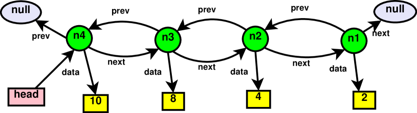
(a) Nodes added (before entering reverse)

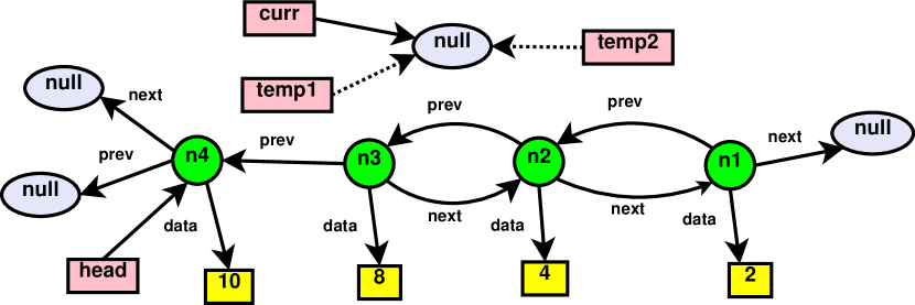
(b) At the end of first loop iteration (without user changes)

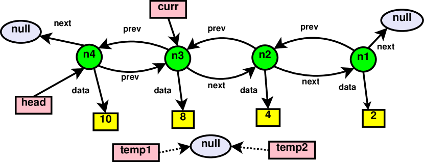
(c) Changes brought about by the user after first loop iteration

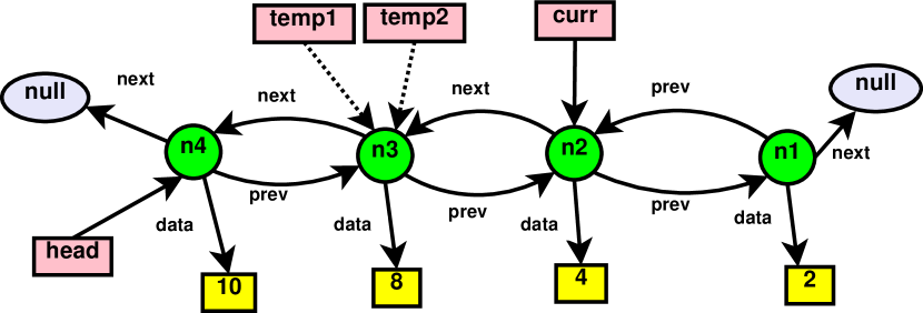
(d) At the end of second loop iteration (after user changes)

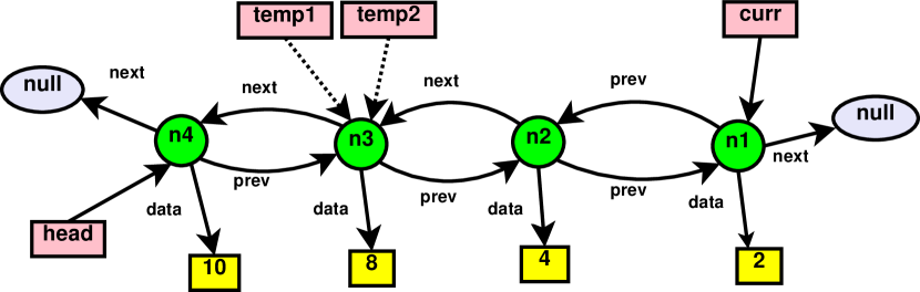
(e) At the end of third loop iteration (no changes required)

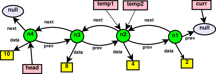
(f) At the end of fourth loop iteration

Figure 2: Visualization of the program execution provided by Wolverine2.

We demonstrate a typical debug-localize-repair session on Wolverine2: the program in Figure 1 creates a doubly linked-list (stack) of four nodes using the push() functions, and then, calls the reverse() function to reverse this list. The reverse() function contains three faults:

1. The loop condition is buggy which causes the loop to be iterated for one less time than expected;

2. The programmer (possibly due to a cut-and-paste error from the previous line) sets temp2 to the prev instead of next field;

3. The head pointer has not been set to the new head of the reversed list.

The programmer uses the start command to launch Wolverine2, followed by four next commands to concretely execute the statements in push() functions, creating the doubly-linked list. Figure 2(a) shows the current (symbolic) state of the program heap, that is displayed to the programmer.

(Wolverine2) start
Starting program...
push(2)
(Wolverine2) next; next; next; next;

push(4);
…

The programmer, then, uses the step command to step into the reverse() function.

reverse();
(Wolverine2) step
current = head;
(Wolverine2) next

The programmer deems the currently displayed state as desirable as this program point and decides to assert it via the spec command. The asserted states are registered as part of the specification, and the repair module ensures that any synthesized program repair does exhibit this program state at this program location.

while(temp1 != NULL)
(Wolverine2) spec
Program states added

Bug1 prevents the execution from entering the while-loop body, the programmer therefore employs enter command to force the execution inside the loop.

while(temp1 != NULL)
(Wolverine2) enter

The programmer issues multiple next commands to reach the end of this loop iteration.

temp1 = current->prev; (Wolverine2) next; next; next; next; next; … while(temp1 != NULL)

The program state at this point (Figure 2(b)) seems undesirable as current and prev field of node n4 point to null (instead of pointing to n3). The programmer corrects the program state by bringing about these changes via the change command.

(Wolverine2) change current n3
(Wolverine2) change n4 -> prev n3

Figure 2(c) shows the updated program state, and the programmer commits them to specification.

(Wolverine2) spec Program states added

The execution is now forced in the loop for the second time, again using the enter command.

(Wolverine2) enter while(temp1 != NULL) …

The state at the end of the second iteration is not correct; the programmer performs the necessary changes and commits it to the specification.

while(temp1 != NULL) (Wolverine2) change current n2 (Wolverine2) change n3 -> prev n2 (Wolverine2) spec Program states added

She then uses the repair command to request a repair patch.

(Wolverine2) repair Repair synthesized...

To repair the program, Wolverine2 first launches its bug localization module that searches for potentially faulty statements; in this case, it identifies the second, third, and fifth statements (lines 7, 6, and 10) in the ‘‘while’’ loop (which is the statement with Bug2) as suspicious candidates.

The repair module, then, searches for possible mutations of the potentially faulty statements (identified by the bug localizer) to synthesize a repair patch that is guaranteed to satisfy the given specifications committed thus far.

In the present case, the repair synthesized by Wolverine2 correctly fixes Bug2; however, the other bugs remain as the trace has not encountered these faults yet. Wolverine2, further, simulates hot-patching of this repair, allowing the user to continue this debugging session rather than having to abort this debug session, recompile, and restart debugging.

To check the generality of the repair, the programmer steps through the third loop iteration to confirm that it does not require a state change, alluding to the fact that the repair patch is possibly correct.

while(temp1 != NULL) (Wolverine2) enter …

The fourth iteration also updates the program heap as per the programmer’s expectations, reinforcing her confidence in the repair patch.

Due to Bug1, the loop termination condition does not hold even after the complete list has reversed; the programmer, thus, forces a change in the control flow via the leave command to force the loop exit.
while(temp1 != NULL) (Wolverine2) leave
Exiting function...

At this point, the programmer notices that the state is faulty as the head pointer continues to point to the node n4 rather than n1, the new head of the reversed list (Figure 2(f)).

The programmer adds this change to the specification and requests another repair patch.

(Wolverine2) change head n1
(Wolverine2) spec Program states added
(Wolverine2) repair Repair synthesized...

This repair requires the insertion of a new statement; Wolverine2 is capable of synthesizing a bounded number of additional statements to the subject program. On our machine, the first repair call takes 0.5 s (fixing Bug2) while the second repair call returns in 0.3 s (fixing Bug1 and Bug3).

To summarize, the debug session builds a correctness specification via corrections to the program state, that Wolverine2 uses to drive automated repair, aided by fault localization to prune the repair space.

2.2 The Claws of Wolverine2

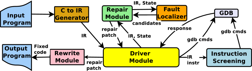
Figure 3: The claws of Wolverine2

The high-level architecture of Wolverine2 is shown in Figure 3. The Driver module is the heart of the tool, providing the user shell and coordinating between other modules.

After receiving a C program, Wolverine2 employs the C-to-IR generator to compile it into its intermediate representation (IR) as a sequence of guarded statements ($\Gamma$) and a location map ($\Lambda$) to map each line of the C-source code to an IR instruction (see §3). Each C-source code instruction can potentially be mapped to multiple IR instructions. For the sake of simplicity, we assume that each C-source code line appears in a new line. Note that each C-code instruction can get compiled down to multiple IR instructions.

The Driver module initiates the debug session by loading the binary on gdb: many of the commands issued by the programmer are handled by dispatching a sequence of commands to gdb to accomplish the task. However, any progress of the program’s execution (for example, the next command from the programmer) is routed via the instruction screening module that manages specification refinement and simulates hot-patching (see §3 and Algorithm LABEL:alg:execute-statement).

On the repair command, the driver invokes the repair module to request an automated repair based on the specification collected thus far. The repair module, in turn, invokes the fault localization engine, to identify a set of suspicious locations. The fault localization algorithm is sound but not complete---though it may return multiple suspicious statements (including ones that are not faulty), the set of these suspicious locations is guaranteed to contain the buggy location. The repair module restricts its mutations within the set of suspicious statements to synthesize a repair patch. This patch is propagated to the instruction screening module to enable hot-patching, enabling the user to continue as if she was executing this transformed program all along. If satisfied, she invokes the rewrite module to translate the intermediate representation of the repaired program to a C language program.

3 Heap Debugging

The state of a program ($\mathcal{S}$) contains a set of variables $\sigma_{V}$ and a set of heap nodes $\sigma_{H}$ with fields $\sigma_{F}$ as $\mathcal{V}\times\mathcal{H}$; the state of the program variables, $\mathcal{V}$, is a map $\sigma_{V}\rightarrow\mathcal{D}$ and the program heap ($\mathcal{H}$) is a map $\sigma_{H}\times\sigma_{F}\rightarrow\mathcal{D}$. The domain of possible values, $\mathcal{D}$, is $\mathcal{I}\cup\sigma_{H}$ where $\mathcal{I}$ is the set of integers. For simplicity, we constrain the discussions in this paper to only two data-types: integers and pointers. We use the function $\Upsilon(e)$ to fetch the type of a program entity; a program entity $e\in\mathcal{E}$ is either a variable $v\in\sigma_{V}$ or a field of a heap node $h\in\sigma_{H}\times\sigma_{F}$. Also, pointers can only point to heap nodes as we do not allow taking reference to variables.

Memory state witnessed by concrete execution via gdb is referred to as the concrete state, from which we extract the symbolic state as a memory graph Zimmermann:2001 , where machine addresses are assigned symbolic names. For our symbolic state, pointers are maintained in symbolic form, whereas scalar values (like integers) are maintained in concrete form. In the concrete state, all entities are maintained in their concrete states.

3.1 Symbolic Encoding of an Execution

⬇

1if (head != NULL) {

2 temp = head->next;

3}

4if (head != NULL

5 || temp != NULL) {

6 return;

7}

8last = head;

9temp = last->next; \end{lstlisting}

10 % \end{minipage}

11 \caption{An example program in C}

12 % \label{fig:IR_motivating_1}

13 \end{subfigure}%

14 ~

15 \begin{subfigure}[t]{0.58\textwidth}

16 \centering

17 % \begin{minipage}{0.80\textwidth}

18 \begin{lstlisting}[language = C]

191 (true) : b0 = (not (head == null))

202 (b0) : temp = head.next

213 (true) : b1 = (head == null)

224 (true) : b2 = (temp == null)

235 (true) : b1 = b1 bor b2

246 (b1) : halt

257 (true) : last = head

268 (true) : temp = last.next \end{lstlisting}

27% \end{minipage}

28 \caption{Intermediate representation of the program}

29 % \caption{Trandformed IR code after bug localization in ~\fig{fig:IR_motivating_1}}

30 % \label{fig:IR_motivating_2}

31 \end{subfigure}

32\caption{Our Intermediate Representation}

33\label{fig:example_IR}

34\end{figure*}

35

36

37We use Hoare triples~\cite{Hoare:1969} to show the semantics of our intermediate representation (\fig{fig:fwd_semantics}). In the intemediate representation, the program is maintained as a sequence of guarded statement, i.e. a statement is executed only if its guard evaluates to {\tt true} at that program point (rules {\tt grd1} and {\tt grd2} in \fig{fig:fwd_semantics}). The scope of our repairs includes modification/insertion of both statements and guards.

38

39% \fig{fig:fwd_semantics} shows the axiomatic semantics of our intermediate representation using Hoare triples~\cite{Hoare:1969}. Our intermediate representation maintains a program as a sequence of {\it guarded statements}: a statement is executed only if the corresponding guard evaluates to {\tt true} (rules {\tt grd1} and {\tt grd2}). The scope of our repairs include the modification/insertion of both the statements and the guards.

40

41Assignment~\mbox{($x:=y$)}, getfield~\mbox{($x:=y.f$)} and putfield~\mbox{($x.f=y$)} are the primary statements in our intermediate representation. For a map $\mathcal{M}$, we use the notation $\mathcal{M}_{1}=\mathcal{M}_{2}[a_{1}\mapsto a_{2}]$ to denote that $\mathcal{M}_{2}$ inherits all mappings from $\mathcal{M}_{1}$ except that the mappings $a_{1}\mapsto a_{2}$ is added/updated. For brevity, we skip discussions of other statements like \var{print}.

42

43\begin{figure*}[t]

44 \scalebox{0.8}{

45 \begin{minipage}{\textwidth}

46 % \begin{align*}

47 \hspace{3em}\infer[asgn]

48 {\opsemf{\langle \mathcal{V}_1, \mathcal{H}_1\rangle}{x\asgn y}{\langle \mathcal{V}_2, \mathcal{H}_1\rangle}}

49 {\Upsilon(x)=\Upsilon(y) & \mathcal{V}_2=\mathcal{V}_1[x\mapsto \mathcal{V}_1(y)]}

50 % \end{align*}

51

52 \begin{align*}

53 \infer[getfld]

54 {\opsemf{\langle \mathcal{V}_1, \mathcal{H}_1\rangle}{x\asgn y.f}{\langle \mathcal{V}_2, \mathcal{H}_1\rangle}}

55 {\Upsilon(x)=\Upsilon(y.f) \quad \Upsilon(y)=\text{ptr} \quad \mathcal{V}_1(y)\neq\text{null} \\ \hfill \mathcal{V}_2=\mathcal{V}_1[x\mapsto \mathcal{H}_1\langle\mathcal{V}_1(y),f\rangle]\hfill} \hspace{1.5em}

56 \infer[putfld]

57 {\opsemf{\langle \mathcal{V}_1, \mathcal{H}_1\rangle}{x.f\asgn y}{\langle \mathcal{V}_1, \mathcal{H}_2\rangle}}

58 {\Upsilon(x)=\Upsilon(y.f) \quad \Upsilon(x)=\text{ptr} \quad \mathcal{V}_1(x)\neq \text{null}\\ \hfill \mathcal{H}_2=\mathcal{H}_1[\langle\mathcal{V}_1(x),f\rangle \mapsto \mathcal{V}_1(y)]\hfill \ }

59 \end{align*}%

60

61 \begin{align*}

62 \infer[cncr]

63 {\opsemf{\langle \mathcal{V}_1, \mathcal{H}_1\rangle}{concrete(\zeta)}{\langle \mathcal{V}_2, \mathcal{H}_1\rangle}}

64 {\hfill \hoarerule{\langle \overline{\mathcal{V}}_1, \overline{\mathcal{H}}_1\rangle}{\zeta}{\langle \overline{\mathcal{V}}_2, \overline{\mathcal{H}}_2 \rangle} \hfill\\ \quad \mathcal{V}_2, \mathcal{H}_2 = Sym(\overline{\mathcal{V}}_2, \overline{\mathcal{H}}_2) \quad \overline{\mathcal{V}}_1, \overline{\mathcal{H}}_1 = Concr(\mathcal{V}_1, \mathcal{H}_1)} \hspace{1.5em} %\hspace{20pt}

65 \infer[skip]

66 {\opsemf{\langle \mathcal{V}_1, \mathcal{H}_1\rangle}{skip}{\langle \mathcal{V}_1, \mathcal{H}_1\rangle}}

67 {}

68 \end{align*}%

69

70 \begin{align*}

71 \infer[grd1]

72 {\opsemf{\langle \mathcal{V}_1, \mathcal{H}_1\rangle}{grd\text{ ? }stmt}{\langle \mathcal{V}_2, \mathcal{H}_2\rangle}}

73 {[\![ grd ]\!]=\text{true} & \hoarerule{\langle \mathcal{V}_1, \mathcal{H}_1\rangle}{\text{stmt}}{\langle \mathcal{V}_2, \mathcal{H}_2\rangle}} \hspace{1.5em}%\hspace{20pt}

74 \infer[grd2]

75 {\opsemf{\langle \mathcal{V}_1, \mathcal{H}_1\rangle}{grd\text{ ? }stmt}{\langle \mathcal{V}_1, \mathcal{H}_1\rangle}}

76 {[\![ grd ]\!]=\text{false}}

77 \end{align*}%

78

79 \begin{align*}

80 \infer[nondet]

81 {\opsemf{\langle \mathcal{V}_1, \mathcal{H}_1 \rangle}{x\asgn nondet}{\langle \mathcal{V}_2, \mathcal{H}_1 \rangle}}

82 {\mathcal{V}_2=\{y\mapsto h\ | \ (h \overset{*}{\gets} \mathcal{H}_1, y=x) \land ((y\mapsto h) \in \mathcal{V}_1, y\neq x)\}} \hspace{1.5em}%\hspace{20pt}

83 \infer[band]

84 {\opsemf{\langle \mathcal{V}_1, \mathcal{H}_1\rangle}{z \asgn x \hspace{3pt} band \hspace{3pt} y}{\langle \mathcal{V}_2, \mathcal{H}_2\rangle}}

85 {{\Upsilon(x)=\Upsilon(y)} & \\ \mathcal{V}_2=\mathcal{V}_1[z\mapsto \mathcal{V}_1(x) \wedge \mathcal{V}_1(y)]}

86 \end{align*}%

87

88 \begin{align*}

89 \infer[bor]

90 {\opsemf{\langle \mathcal{V}_1, \mathcal{H}_1\rangle}{z \asgn x \hspace{3pt} bor \hspace{3pt} y}{\langle \mathcal{V}_2, \mathcal{H}_2\rangle}}

91 {\Upsilon(x)=\Upsilon(y) & \mathcal{V}_2=\mathcal{V}_1[z\mapsto \mathcal{V}_1(x) \vee \mathcal{V}_1(y)]} \hspace{1.5em}% \hspace{20pt}

92 \infer[bassign]

93 {\opsemf{\langle \mathcal{V}_1, \mathcal{H}_1\rangle}{z = x \hspace{3pt} \star \hspace{3pt} y}{\langle \mathcal{V}_2, \mathcal{H}_2\rangle}}

94 {\Upsilon(x)=\Upsilon(y) & \mathcal{V}_2=\mathcal{V}_1[z\mapsto [\mathcal{V}_1(x) \star \mathcal{V}_1(y)]]\\ &\star \in \{=, \neq, <, >, \leq, \geq\}}

95 \end{align*}%

96

97 \end{minipage}

98 }

99 \caption{\textbf{Forward Semantics} of our intermediate representation}

100 \label{fig:fwd_semantics}

101\end{figure*}

102

103Each statement comes with its set of preconditions that must be satisfied for the update to ensue, for example, the assignment statement requires that the type of the variables match, and a getfield statement requires type matching along with the need for the dereferenced variable to be a pointer and non-\var{null}.

104

105% The assignment statement requires a precondition that the types of the variables match; if the precondition holds, it updates the variable map $\mathcal{V}_{1}$ by adding a new mapping from the assigned variable \var{x} to the current value contained in \var{y}. The getfield statement requires type consistency and also that the dereferenced variable should be of pointer type and non-\var{null}. If the preconditions are met, the respective update ensues. {sec:spec_refine}

106

107We use \var{concrete} statement to allow an interesting debugging strategy (referred to as \textit{specification refinement}, see \sect{sec:spec_refine}). For such statements, $\zeta$, we extract a concrete precondition, execute $\zeta$ \textit{concretely} and fetch a concrete postcondition for \var{concrete} statement.

108

109% The \var{concrete} statement is used to enable an interesting debugging strategy (we refer to it as \textit{specification refinement}): we invoke \var{concrete} with statement(s) $\zeta$ that we do not wish to model symbolically. We, in this case, extract a concrete precondition, execute $\zeta$ {\textit{concretely}} on the precondition, fetching a concrete postcondition. The symbolic state corresponding to the concrete postcondition is assumed to be the postcondition of the \var{concrete} statement.

110

111The guards are predicates that can involve comparisons from \{$\leq,<,\geq,>,=,\neq$\} for integers and only \{$=,\neq$\} for pointers (we omit their formal semantics).

112

113The boolean predicates for the guards can be constructed using the boolean assignment statement ($z=x\star y$, where $\star\in\{=,\neq,<,>,\leq,\geq\}$); compound conditions over these predicates are constructed via the boolean-or operator ($z:=x\ \textrm{bor}\ y$) or the boolean-and operator ($z:=x\ \textrm{band}\ y$). The program also allows for \textit{non-deterministic} assignments ($x:=nondet$).

114\fig{fig:example_IR} shows a program with compound conditions and its intermediate representation. % new

115

116When the \underline{{\tt repair}} command is invoked at a particular program point $p$, by the conjunction of the semantic encoding of the instructions in the trace, the \textit{repair module} constructs a symbolic model, $\Phi_{sem}$, of the execution trace upto~$p$ (we assume that the trace has a length of \textit{n}).

117

118% When the \underline{{\tt repair}} command is invoked (say after executing~{\tt n} IR instructions via {\tt gdb}), the \textit{repair module} constructs the semantic model of the execution trace, $\Phi_{sem}$, by the conjunction of the semantic encoding of the instructions in the trace:

119

120{\centering

121 $\displaystyle\begin{aligned} \Phi_{sem}\equiv\prod^{n}_{i=1}\mathcal{T}_{i}(\mathcal{S}_{i},\mathcal{S}_{i+1})\end{aligned}\par$

122\par}

123%Necessary for centering to work

124

125\noindent $\mathcal{T}_{i}$ encodes the semantics of the $i^{th}$ instruction (\fig{fig:fwd_semantics}) and $\mathcal{S}_{i}$ (and $\mathcal{S}_{i+1}$) denote the input (and output) state of this instruction (respectively).

126

127

128%\toolname can synthesize both statements as well as conditionals for if-then-blocks.

129

130

131\subsection{The Heap Debugger}

132

133%\RestyleAlgo{boxruled}

134%\AlgoDisplayB\xikMarkers\AlgoDisplayGroupMarkers\SetAlgoB\xikMarkers{ \{}{ \}\ }%

135%\SetAlgoNoEnd\SetAlgoNoLine

136

137\RestyleAlgo{boxruled}

138%\AlgoDisplayB\xikMarkers\AlgoDisplayGroupMarkers\SetAlgoB\xikMarkers{ \{}{ \}\ }%

139%\SetAlgoNoEnd\SetAlgoNoLine

140\begin{algorithm}[t]

141\caption{\label{alg:heap-debugger}The Heap Debugger}

142$\Theta=\{e|e\in\mathcal{H}\}$\\

143\While{true}{

144 $cmd\mathrel{:}=Prompt()$\\

145 \Switch{cmd}{

146 \uCase{\texttt{start}}{loc = gdb\_start()}

147 \uCase{\texttt{next}}{loc = ExecuteStatement(\texttt{loc})\\ $\mathcal{S}_{c}$ = fetch\_concrete\_state() \\ $\mathcal{S}_{s},\gamma$ = create\_symbolic\_state($\mathcal{S}_{c},\gamma$) \\ display\_map($\mathcal{S}_{s}$)}

148 \uCase{\texttt{break <loc>}}{gdb\_send(\texttt{break <loc>)}}

149 % \uCase{\texttt{track <[addlst]> <[remlst]>}}{$\Theta\mathrel{:}=\Theta\cup addlst\setminus remlst$}

150 \uCase{\texttt{change <$e_{s}$> <$v_{s}$>}}{$\mathcal{S}_{c}$ = fetch\_concrete\_state() \\ $\mathcal{S}_{s},\gamma$ = create\_symbolic\_state($\mathcal{S}_{c},\gamma$) \\ $\mathcal{S}_{s}[e_{s}]\mathrel{:}=v_{s}$ \\ $gdb\_set\_address(\gamma[e_{s}],v_{s})$}

151 \uCase{\texttt{spec}}{$\mathcal{S}_{c}$ = fetch\_concrete\_state() \\ $\mathcal{S}_{s},\gamma$ = create\_symbolic\_state($\mathcal{S}_{c},\gamma$) \\ $assert\_spec(\Lambda[loc].IR\_id,\mathcal{S}_{s}\cap\Theta)$}

152 \uCase{\texttt{repair}}{$\texttt{patch}\mathrel{:}=repair\_run()$\\ hot\_patch(\var{patch})}

153 }

154}

155\end{algorithm}

156

157\RestyleAlgo{boxruled}

158%\AlgoDisplayB\xikMarkers\AlgoDisplayGroupMarkers\SetAlgoB\xikMarkers{ \{}{ \}\ }%

159%\SetAlgoNoEnd\SetAlgoNoLine

160\begin{algorithm}[t]

161% \Fn{LL1Parse}{

162 \KwIn {$\Gamma::[\langle stmt.action,stmt.grd,stmt.loc]$, \\ \hspace{30pt}$\Lambda::N\rightarrow\langle L,\{changed,inserted,preserved\}\rangle$}

163 \caption{\label{alg:execute-statement}ExecuteStatement}

164 \uIf{stmt == "concrete"}{

165 loc = gdb\_send("next")\\

166 $\mathcal{S}_{c}$ = fetch\_concrete\_state() \\ $\mathcal{S}_{s},\gamma$ = create\_symbolic\_state($\mathcal{S}_{c},\gamma$) \\

167 repair\_add\_spec($\Gamma[pp].IR\_id,\mathcal{S}_{s}\cap\Theta$)

168 } \uElseIf{$\Lambda[loc].status==changed$} {

169 gdb\_send("skip")\\

170 irstm = IR2gdbStm($\Lambda[loc].IR\_id$)\\

171 gdb\_exec\_stm(irstm)

172 } \uElseIf{$\Lambda[loc].status==inserted$} {

173 irstm = IR2gdbStm($\Lambda[loc].IR\_id$)\\

174 gdb\_exec\_stm(irstm)

175 } \lElse {

176 loc = gdb\_send("next")

177 }

178 \Return loc

179\end{algorithm}

180

181\alg{alg:heap-debugger} provides a high-level sketch of the operation of \toolname. Our algorithm accepts a program as a sequence of guarded statements $\langle\pi,\omega\rangle$ where $\pi$ is a {\it guard} predicate of the form $\langle op,arg1,arg2\rangle$, and $\omega$ can be one of assignment, getfield, putfield, boolean-or, boolean-and, booelan-assign, non-deterministic or concrete statement. %is either an assignment ($v_{1}=v_{2}$), a getfield operation ($v_{1}=v_{2}.\textit{field}$), a putfield operation ($v_{1}.\textit{field}=v_{2}$), a $concrete$ statement.

182

183Before the algorithm enters the command loop, $\Theta$ is initialized to the set of entities in the program; these entities are recorded whenever \underline{\var{spec}} is invoked.

184

185% \toolname starts off with a string of initializations, where $\Theta$ is the set of ‘tracked" entities: the state of only these entities is recorded while creating the specifications. The algorithm, then, enters the command loop. When next command is invoked, Wolverine2 dispatches the next program statement to be executed (at source line loc) to the statement screening module (Algorithm LABEL:alg:execute-statement), which returns the next C-code source line to be executed. After execution, Wolverine2 uses the function fetch_concrete_state() to query gdb for the updated program state, and then generates the memory map Zimmermann:2001 (using the create_symbolic_state() function). This function returns the symbolic map $\mathcal{\widehat{S}}$ and a map $\gamma$; the map $\gamma$ records the mapping of the concrete entities to their symbolic forms. The symbolic memory map is displayed to the programmer as a visual aid for debugging (see §1). The functionality of break command is similar to the default instruction in gdb: for inserting a breakpoint. The change command allows the programmer to convey expectations of the desired program state at a point. The program state can be changed by providing a new value $v_{s}$ to a symbolic state $e_{s}$. Wolverine2 fetches the relevant concrete state and issues multiple commands (summarized by the function gdb_set_address()) to modify the concrete program state. The spec command asserts the symbolic state at the current program point. Finally, the repair command invokes the repair module, which attempts to synthesize a repair patch that satisfies the concatenated assertions added thus far. The repair module internally calls the fault localizer and, hence, fault localization is not available as an explicit command. If the repair succeeds, the repair patch is passed to the instruction screening module, which simulates hot-patching for a seamless debugging session. In addition to the above, Wolverine2 also supports altering of the control flow (like entry/exit of loops via the enter and leave commands respectively), flip branch directions etc. We demonstrated these features in §1 but we omit the details. The ExecuteStatement() function, provided by the instruction screening module, is described in Algorithm LABEL:alg:execute-statement; this function accepts a list of guarded statements $\Gamma$ and a map $\Lambda$ from the source line numbers (in $N$) to a tuple containing the corresponding IR instruction(s) (in $L$). Status bits ($F\in\{changed,inserted,preserved\}$) are used to indicate if: (a) the IR instruction has been modified ($changed$) by a repair patch, (b) appears as a new instruction ($inserted$) due to a repair patch, or (c) is unmodified ($preserved$); this information is required to simulate hot-patching. Deletion of a statement is also marked ($changed$); the corresponding patch simply sets the guard of the instruction to false. The instruction screening module handles two primary tasks: • Handling concrete statements. Upon encountering a concrete statement, Wolverine2 executes it via gdb by issuing the next command. The effect of this concrete execution is then asserted by taking a snapshot of the updated concrete state (again via gdb) and adding the corresponding symbolic state to the specification. We refer to this debugging strategy as specification refinement (see §6.1). • Simulate hot-patching. If a repair patch has modified the statement, Wolverine2 requests gdb to skip the execution of this statement, and translates the ‘‘effect" of the modification into a string of gdb commands ($irstm$) via the IR2gdbStm() function and consigns the command-list to gdb using the gdb_exec_stm() function. Otherwise, the next statement is concretely executed via gdb by issuing the next command.

4 Proof-Guided Repair

1 $\Phi_{grd}=\Phi_{stm}=\Phi_{ins}=\emptyset$ 2 $n\mathrel{:}=|\mathcal{P}|+num\_insert\_slots$ /* Assert the input (buggy) program */ 3 for $i\in\{1\dots|\mathcal{P}|\}$ do 4       if $i\in\mathcal{L}$ then 5             $\Phi_{grd}\mathrel{+}=\langle\widehat{\mathcal{P}}.grd[\xi(i)]==\mathcal{P}.grd[i]\rangle$ 6             $\Phi_{stm}\mathrel{+}=\langle\widehat{\mathcal{P}}.stm[\xi(i)]==\mathcal{P}.stm[i]\rangle$ 7             8      else 9             $\Phi_{grd}\mathrel{+}=\langle\lnot r_{\xi(i)}\implies(\widehat{\mathcal{P}}.grd[\xi(i)]==\mathcal{P}.grd[i])\rangle$ 10             $\Phi_{stm}\mathrel{+}=\langle\lnot s_{\xi(i)}\implies(\widehat{\mathcal{P}}.stm[\xi(i)]==\mathcal{P}.stm[i])\rangle$ 11             12       end if 13       14 end for /* Initialize the insertion slots */ 15 for $i\in\{|\mathcal{P}|\dots n\}$ do 16       $\Phi_{ins}\mathrel{+}=\langle\lnot t_{\xi(i)}\implies(\phi_{\xi(i)}==\texttt{false})\rangle$ 17       18 end for /* Define the placing function $\xi$ */ 19 $\Phi_{bk}\mathrel{:}=\forall_{i\in\{1\dots n\}}(1\leq\xi(i)\leq n)\land\texttt{distinct}({\xi(i)})$ 20 $\Phi_{bk}\mathrel{+}=\forall_{\langle i,.,.\rangle,\langle k,.,.\rangle\in\mathcal{P}}(i<k\implies\xi(i)<\xi(k))$ 21 $v\mathrel{:}=\textsc{UNSAT}$ /* Relax till specification is satisfied */ 22 $\tau_{grd}\mathrel{:}=\tau_{stm}\mathrel{:}=\tau_{ins}\mathrel{:}=0$ 23 while $v=\textsc{UNSAT}$ or tries exceeded do 24       $\langle res,\widehat{\mathcal{P}},uc\rangle\mathrel{:}=\textsc{Solve}(\Phi_{spec}\land\Phi_{sem}\land\Phi_{bk},$ 25                          $\Phi_{grd}\land\Sigma_{k\in\{1\dots|\mathcal{P}|\}}r_{k}<\tau_{grd},$ 26                          $\Phi_{stm}\land\Sigma_{k\in\{1\dots|\mathcal{P}|\}}s_{k}<\tau_{stm}$ 27                          $\Phi_{ins}\land\Sigma_{k\in\{|\mathcal{P}|+1\dots n\}}t_{k}<\tau_{ins})$        /* Use the UNSAT core to drive relaxation */ 28       if $res=\textsc{UNSAT}$ then 29             if $\Phi_{grd}\cap uc\neq\emptyset$ then  $\tau_{grd}\mathrel{+}=1$ ; 30             else if $\Phi_{stm}\cap uc\neq\emptyset$ then  $\tau_{stm}\mathrel{+}=1$ ; 31             else if $\Phi_{ins}\cap uc\neq\emptyset$ then  $\tau_{ins}\mathrel{+}=1$ ; 32             else  return null ; 33             34       35 end while 36if tries exceeded then  return null ; return $\widehat{\mathcal{P}}$ Algorithm 1 Unsat Core Guided Repair Algorithm Algorithm 1 shows our repair algorithm: it takes a (buggy) program $\mathcal{P}$ as a sequence of guarded statements, a set of locked locations $\mathcal{L}$, and a bound on the number of new statements that a repair is allowed to insert (num_insert_slots). The repair algorithm attempts to search for a repair candidate $\widehat{\mathcal{P}}$ (of size $n=|\mathcal{P}|+\texttt{num\_insert\_slots}$) that is ‘‘close" to the existing program and satisfies the programmers expectations (specification). Our algorithm is allowed to mutate and delete existing statements and insert at most $n$ new statements; however, mutations are not allowed for the locations contained in $\mathcal{L}$. The insertion slots contain a guard \var{false} to begin with~(Line 8); the repair algorithm is allowed to change it to ‘activate" the statement. Deletion of a statement changes the guard of the statement to false. Wolverine2 allows for new nodes and temporary variables by providing a bounded number of additional (hidden) nodes/temporaries, made available on demand. The programmer configures the number of insertion slots, but these slots are activated by the repair algorithm only if needed. For loops, we add additional constraints so that all loop iterations encounter the same instructions.

4.1 Primary Constraints

We use a set of selector variables $\{r_{1},\dots,r_{n},s_{1},\dots,s_{n}\}$ to enable a repair. Setting a selector variable to true relaxes the respective statement, allowing Wolverine2 to synthesize a new guard/statement at that program point to satisfy the specification. We define a metric, $closeness(\mathcal{P}_{1},\mathcal{P}_{2})$, to quantify the distance between two programs by summing up the set of guards and statements that match at the respective lines. As the insertion slots should be allowed to be inserted at any point in the program, the closeness metric would have to be ‘adjusted to incorporate this aberration due to insertions. For this purpose, our repair algorithm also infers a relation $\xi$ that maps the instruction labels in the repair candidate $\widehat{\mathcal{P}}$ to the instruction labels in the original program $\mathcal{P}$; the instruction slots are assigned labels from the set $\{|\mathcal{P}|+1,\dots,n\}$. We define our closeness metric as:

186

187\vspace{2pt}

188

189\begin{align*}

190%{ \centering

191% $\displaystyle\texttt{closeness}(\mathcal{P},\widehat{\mathcal{P}})=&\sum_{i=1}^{|\mathcal{P}|}(\mathcal{P}.grd[i]=\widehat{\mathcal{P}}.grd[\xi(i)])\\ +\sum_{i=1}^{|\mathcal{P}|}(\mathcal{P}.stm[i]=\widehat{\mathcal{P}}.stm[\xi(i)])\\ +\sum_{i=|\mathcal{P}|+1}^{n}(\widehat{\mathcal{P}}.grd[\xi(i)]\neq\texttt{false})$

192%\par}%Necessary for centering to work

193\end{align*}

194\vspace{2pt}

195

196The above metric weights a repair candidate by the changes in the statements/guards and new statements added (insertion slots {\it activated}).

197

198\alg{alg:repair} starts by asserting the input program $\mathcal{P}$, via the selector variables if it is not a locked location, as part of the constraints $\Phi_{grd}$ and $\Phi_{stm}$ (lines~3--11), and initializes the insertion slots to their deactivated state (lines~12--14) with selector variables $t_{i}$. The constraint $\Phi_{bk}$ ensures that the function $\xi$ is well-formed: for each $i$, $\xi(i)$ is a distinct value in the range $\{1\dots n\}$ and is a monotonically increasing function (this ensures that the statements preserve the same order in $\widehat{\mathcal{P}}$ as the order in $\mathcal{P}$).

199

200Finally, it uses issues a \textsc{Solve()} query to an SMT solver to solve the repair constraint; the sub-constraint $\Phi_{sem}$ contains the semantic encoding of our intermediate statements (\fig{fig:fwd_semantics}) and $\Phi_{spec}$ contains the specification collected during the debugging session as a result of the \underline{\var{spec}} commands.

201

202

203\subsection{Proof-Guided Search Space Widening}

204

205To ensure that the repaired candidate program $\widehat{\mathcal{P}}$ is \textit{close} to the original program, we progressively relax the closeness bounds. The variables $\tau_{grd},\tau_{stm},$ and $\tau_{ins}$ constrain the distance (in terms of changed guards, statements and activated insertion slots) of a repair candidate from the original program.

206

207We use a {\it Proof-Guided Repair Strategy}: the unsat core ($uc$) produced from the proof of unsatisfiability directs us to the bound that needs to be relaxed. The unsat core represents the central {\it reason} as to why the program cannot be made to satisfy the specification; if a constraint $\langle s_{i}\implies\dots\rangle$ is found in the unsat core, it implies that the reason for unsatisfiability {\it may} be attributed to the fact that $s_{i}$ is false! Hence, one possible way to remove this unsatisfiability is to increase the bound on $\tau_{stm}$ that allows $s_{i}$ to turn \var{false}.

208

209At the same time, we would also like to enforce a priority on the relaxations; for instance, deletion of a statement or mutation of a guard can be considered ‘smaller" changes than changing a statement, or worse, inserting a new statement. The chain of conditions (lines 25--27) ensures that, if the unsat core directs us to a possibility of smaller change, we relax the respective bound before others. Finally, on a successful repair, we return the repaired program $\widehat{\mathcal{P}}$. Guiding repair via the unsat proof has multiple advantages: • The unsatisfiability core (uc) guides us to a feasible repair; for example, if $uc$ does not contain the constraints pertaining to activation of the insertion slots, then it is unlikely that inserting a new statement will fix the bug; • It allows us to prioritize the repair actions; one would prefer mutation of a statement than the insertion of a new statement; • The strategy is fast as the solver operates on a constrained search space that is incrementally widened (in a direction dictated by the proofs) as the search progresses. In case the program to be repaired is close to the original program, the solver will be provided only ‘‘easy" instances that are allowed to mutate/insert a small number of statements; • It allows a fail-fast (line 28) if the specification is buggy or the repair is not possible due to structural constraints (like the number of insertion slots provided); if $uc$ does not contain any constraint from {$\Phi_{grd},\Phi_{stm},\Phi_{ins}$}, then the program cannot be repaired via any repair action without violating the hard constraints (like the program semantics). The unsat core not only identifies the possible culprits (a sort of bug localization) but also allows us to define a priority among our repair preferences. To the best of our knowledge, ours is the first repair algorithm that uses unsat proofs to direct repair; however, this idea has threads of similarity with a model-checking algorithm, referred to as underapproximation wideningGrumberg:2005 (see §8). We evaluated a variant (AlgVar) of our proof directed repair scheme: instead of increasing the respective repair bound, we randomly relax one of the constraints from the unsat core. However, we found that the unsat cores are poor---quite far from the minimum unsat core. Hence, this variant of our algorithm performs poorly, both in terms of success rate and the time taken for repair (see §7).

5 Bug localization

The objective of our bug localization module is to identify a (small) set of statements that are likely to contain the fault(s). Our algorithm is targeted at localizing faults for use by the repair phase of Wolverine2: our localization algorithm localizes faults on concrete program traces using the assertions as precondition/postcondition pairs. The bug localization phase exposes two primitives to the repair phase: • Statement locks: Adding a ‘‘locked" attribute to a statement asserts the statement in its position; • Non-deterministic assignment: A non-deterministic assignment allows us to assign an angelic value.

Definition 1

(Upward exposed statement) A statement whose left-hand side expression (variable or field definition) or its alias has not been assigned by any preceding program statement.

Definition 2

(Downward exposed statement) A statement whose left-hand side expression (variable or field definition) or its alias has not been assigned by any following program statement.

Definition 3

(Sandwiched statement) A statement that is neither upward exposed nor downward exposed.

5.1 Intuition

In this section, we provide the intuition behind our localization algorithm with a few examples.

5.1.1 Program with a single bug and semantically independent statements

implies that the value is indeterminate.}

210% % \scalebox{0.7}{

211% \begin{tabularx}{\textwidth}{| X | c | X || X | c |}

212% \toprule

213% Forward & Program & Backward & Execution of & Difference\\

214% Execution & & Execution & correct program & \\ \midrule

215% PreCondition: [a:n1, b:n2, c:n3, d:n5] & & [a:n1, b:n2, c:n3] & & 0\\ \hline

216% & a = a.next & & & \\ \hline

217% [a:n2, b:n2, c:n3] & & [a:n2, b:n2, c:n3] & [a:n2, b:n2, c:n3] & 0 \\ \hline

218% & b = b.next \textcolor{blue}{(fix: b = d)} & & & \\ \hline

219% [a:n2, b:n3, c:n3] & & [a:n2, b:n5, c:n3] & [a:n2, b:n5, c:n3] & \textcolor{red}{1}\\ \hline

220% & c = c.next & & & \\ \hline

221% [a:n2, b:n3, c:n4] & &PostCondition: [a:n2, b:n5, c:n4, d:n5] & [a:n2, b:n5, c:n4] & 1\\

222% \bottomrule

223% \end{tabularx}

224% % }

225% \label{tab:single_bug_inde_ue}

226% \end{table*}

227% \vspace{-1em}

228

229\begin{table}[t]

230 \centering

231 \caption{Single bug in a program with semantically independent statements.

232 We show states as a tuple with the values of variables $\langle a,b,c,d\rangle$.} % ? implies that the value is indeterminate.}

233 % \begin{tabular}{| c | c || c | c |}

234 \begin{tabularx}{0.95\textwidth}{ C | C || c | c || C }

235 \toprule

236 \rowcolor{lightgray}

237 Forward & Backward & Diff. & Grad. & Correct Execution \\

238 \midrule

239 \midrule

240 \makecell{\textcolor{blue}{(precondition)}\\ $\langle n_{1},n_{2},n_{3},n_{5}\rangle$} & $\langle n_{1},n_{2},n_{3},n_{5}\rangle$ & 0 & & \\ \hline

241 \rowcolor{arylideyellow}

242 \multicolumn{3}{c}{a = a.next} & 0 & \\ \hline

243 $\langle n_{2},n_{2},n_{3},n_{5}\rangle$ & $\langle n_{2},n_{2},n_{3},n_{5}\rangle$ & 0 & & $\langle n_{2},n_{2},n_{3},n_{5}\rangle$ \\ \hline

244 \rowcolor{arylideyellow}

245 \multicolumn{3}{c}{b = b.next \textcolor{blue}{(fix: b = d)}} & 1 & \\ \hline

246 $\langle n_{2},n_{3},n_{3},n_{5}\rangle$ & $\langle n_{2},n_{5},n_{3},n_{5}\rangle$ & \textcolor{red}{1} & & $\langle n_{2},n_{5},n_{3},n_{5}\rangle$ \\ \hline

247 \rowcolor{arylideyellow}

248 \multicolumn{3}{c}{c = c.next} & 0 & \\ \hline

249 $\langle n_{2},n_{3},n_{4},n_{5}\rangle$ & \makecell{\textcolor{blue}{(postcondition)}\\ $\langle n_{2},n_{5},n_{4},n_{5}\rangle$} & \textcolor{red}{1} & & $\langle n_{2},n_{5},n_{4},n_{5}\rangle$ \\

250 \bottomrule

251 \end{tabularx}

252 \label{tab:single_bug_inde_ue}

253\end{table}

254

255% \noindent

256% [Fwd: a:n2, b:n2, c:n3] a = a.next [Back: a:n2, b:n2, c:n3] [Correct State: a:n2, b:n2, c:n3]\\ \

257% 2. b = b.next (correction: b = d) \\ \

258% [Fwd: a:n2, b:n3, c:n3] [Back: a:n2, b:n5, c:n3] [CorrectFwd: a:n2, b:n5, c:n3]\\ \

259% 3. c = c.next \\ \

260% [Fwd: a:n2, b:n3, c:n4] [Back: a:n2, b:n5, c:n4] [CorrectFwd: a:n2, b:n5, c:n4] \\ \

261% PostCondition: [a:n2, b:n5, c:n4] \\ \

262Consider the program shown in the second column of \tab{tab:single_bug_inde_ue}: in this case, all the statements are semantically independent, i.e., there does not exist any true dependencies among the statements. To understand the situation, let us also consider the states in the correct execution.

263The reader should be able to understand the state updates for the forward execution intuitively (first column); the details are discussed in \S\ref{fwd_execution}.

264

265The backward execution (third column) is an attempt at matching the correct execution---we commence from the postcondition, and ‘copy" states from the precondition whenever the assigned variable is upward exposed. Let us illustrate how the backward execution is performed: the backward execution commences from the postcondition and moves towards the precondition (it is essentially the weakest precondition computation, but under the assumption that some of the states could be buggy). For arriving at the backward execution state at the third statement, it checks if c is upward exposed, i.e., if it has a preceding assignment statement that assigns to the variable c. As there is no such statement, it simply reads the state for c from the precondition. The same happens for the other statements. In this case, the backward execution exactly matches the states from the execution of the correct program (fourth column). Now, one can see that the forward execution states agree with backward execution states at statements before the buggy statement, upon whose execution the difference between forward and backward execution builds up. The statement where this difference starts to build up is precisely the buggy location. implies that the value is indeterminate.}

266% % \scalebox{0.8}{

267% % \begin{tabular}{| c | c | c || c | c |}

268% \begin{tabularx}{\textwidth}{| X | c | X || X | c |}

269% \toprule

270% Forward & Statement & Backward & Execution of & Difference\\

271% Execution & & Execution & correct program & \\

272% \midrule

273% PreCondition: [a:n1, b:n2, c:n3, d:n1] & & [a:n1, b:n2, c:n3] & & 0\\ \hline

274% & b = a.next & & & \\ \hline

275% [b:n2, c:n3] & & [(b:n1, c:n3), (b:n2, c:n3), (b:n3, c:n3)] & [b:n2, c:n3] & 0 \\ \hline

276% & b = b.next \textcolor{blue}{(fix: b = d)} & & & \\ \hline

277% [b:n3, c:n3] & & [b:n2, c:n3] & [b:n1, c:n3] & \textcolor{red}{1}\\ \hline

278% & c = c.next & & & \\ \hline

279% [b:n3, c:n4] & & PostCondition :[b:n1, c:n4] & [b:n1, c:n4] & 1\\

280% \bottomrule

281% \end{tabularx}

282% % }

283% \label{tab:single_bug_notUE}

284% \end{table*}

285

286\begin{table}[t]

287 \centering

288 \caption{Single bug program with semantically independent but not upward exposed statements.

289 We show states as a tuple with the values of variables $\langle a,b,c,d\rangle$.} % ? implies that the value is indeterminate.}

290 % \scalebox{0.8}{

291 % \begin{tabular}{| c | c || c | c |}

292 \begin{tabularx}{0.95\textwidth}{ C | C || c | c || C }

293 \toprule

294 \rowcolor{lightgray}

295 Forward & Backward & Diff. & Grad. & Correct Execution \\

296 \midrule

297 \midrule

298 \makecell{\textcolor{blue}{(precondition)}\\ $\langle n_{1},n_{2},n_{3},n_{5}\rangle$} & $\langle n_{1},n_{2},n_{3},n_{5}\rangle$ & 0 & & \\ \hline

299 \rowcolor{arylideyellow}

300 \multicolumn{3}{c}{b = a.next} & 0 & \\ \hline

301 $\langle n_{1},n_{2},n_{3},n_{5}\rangle$ & $\langle n_{1},n_{1},n_{3},n_{5}\rangle$, $\langle n_{1},n_{2},n_{3},n_{5}\rangle$, $\langle n_{1},n_{3},n_{3},n_{5}\rangle$, $\langle n_{1},n_{5},n_{3},n_{5}\rangle$ & 0 & & $\langle n_{1},n_{2},n_{3},n_{5}\rangle$ \\ \hline

302 \rowcolor{arylideyellow}

303 \multicolumn{3}{c}{b = b.next \textcolor{blue}{(fix: b = d)}} & 1 & \\ \hline

304 $\langle n_{1},n_{3},n_{3},n_{5}\rangle$ & $\langle n_{1},n_{5},n_{3},n_{5}\rangle$ & \textcolor{red}{1} & & $\langle n_{1},n_{5},n_{3},n_{5}\rangle$ \\ \hline

305 \rowcolor{arylideyellow}

306 \multicolumn{3}{c}{c = c.next} & 0 & \\ \hline

307 $\langle n_{1},n_{3},n_{4},n_{5}\rangle$ & \makecell{\textcolor{blue}{(postcondition)}\\ $\langle n_{1},n_{5},n_{4},n_{5}\rangle$} & \textcolor{red}{1} & & $\langle n_{1},n_{5},n_{4},n_{5}\rangle$ \\

308 \bottomrule

309 \end{tabularx}

310 \label{tab:single_bug_notUE}

311\end{table}

312

313The procedure differs when a statement is not upward exposed: for the program shown in second column of \tab{tab:single_bug_notUE}, the statements are not \textit{upward exposed} (first and second statement assign to the same variable \var{b}).

314Due to the previous update, it cannot be determined what would be the state when such a statement is run through a backtrackward traversal (as discussed above).

315In such a situation, we split the states, assigning all possible nodes in the data-structure to the concerned variable (here \var{b}), in the hope that at least one of them would be a state agreeing with the execution of the correct program.

316

317 We can compute the difference between two states by the number of variables whose values \textit{disagree} amongst these states. We can define a gradient of the difference along between two traces $t_{1}$ and $t_{2}$ (of same length) by:

318

319 \begin{itemize}

320 \item Computing a differential trace $\delta t$ by computing the difference between the corresponding states in $t_{1}$ and $t_{2}$;

321 \item Finding a gradient of the differential trace, $\partial(\delta t)$, by computing $(\partial(\delta t))_{i}=||(\delta t)_{i}-(\delta t)_{i+1}]||$, i.e. computing the distance between two corresponding trace elements. For a trace (sequence) $t$, we use $t_{i}$ to refer to its $i^{th}$ element.

322 \end{itemize}

323

324

325

326 For our example, there are points where there is a \textit{non-zero gradient of difference} between states in forward and backward execution at one location--exactly the buggy statement (in the given example).

327

328\subsubsection{Program with a single bug and semantically dependent statements}

329

330% PreCondition: [a:n1, b:n2, c:n3] \\ \

331% 1. a = a.next \\ \

332% [Fwd: a:n2, b:n2, c:n3] [Back: a:n2, b:n2, c:n3] [CorrectFwd: a:n2, b:n2, c:n3]\\ \

333% 2. b = b.next (correction: b = d) \\ \

334% [Fwd: a:n2, b:n3, c:n3] [Back: a:n2, b:n5, c:n3] [CorrectFwd: a:n2, b:n5, c:n3]\\ \

335% 3. c = b.next \\ \

336% [Fwd: a:n2, b:n2, c:n4] [Back: a:n2, b:n5, c:n6] [CorrectFwd: a:n2, b:n5, c:n6]\\ \

337% PostCondition: [a:n2, b:n5, c:n6]

338

339

340\begin{table}[t]

341 \centering

342 \caption{Single bug program with semantically dependent and not upward exposed statements. We show states as a tuple with the values of variables $\langle a,b,c,d\rangle$.} % ? implies that the value is indeterminate.}

343 % \scalebox{0.8}{

344 % \begin{tabular}{| c | c || c | c |}

345 \begin{tabularx}{0.95\textwidth}{ C | C || c | c || C }

346 \toprule

347 \rowcolor{lightgray}

348 Forward & Backward & Diff. & Grad. & Correct Execution \\

349 \midrule

350 \midrule

351 \makecell{\textcolor{blue}{(precondition)}\\ $\langle n_{1},n_{2},n_{3},n_{5}\rangle$} & $\langle n_{1},n_{2},n_{3},n_{5}\rangle$ & 0 & & \\ \hline

352 \rowcolor{arylideyellow}

353 \multicolumn{3}{c}{a = a.next} & 0 & \\ \hline

354 $\langle n_{2},n_{2},n_{3},n_{5}\rangle$ & $\langle n_{2},n_{2},n_{3},n_{5}\rangle$ & 0 & & $\langle n_{2},n_{2},n_{3},n_{5}\rangle$ \\ \hline

355 \rowcolor{arylideyellow}

356 \multicolumn{3}{c}{b = b.next \textcolor{blue}{(fix: b = d)}} & 1 & \\ \hline

357 $\langle n_{2},n_{3},n_{3},n_{5}\rangle$ & $\langle n_{2},n_{5},n_{3},n_{5}\rangle$ & \textcolor{red}{1} & & $\langle n_{2},n_{5},n_{3},n_{5}\rangle$ \\ \hline

358 \rowcolor{arylideyellow}

359 \multicolumn{3}{c}{c = b.next} & 1 & \\ \hline

360 $\langle n_{2},n_{3},n_{4},n_{5}\rangle$ & \makecell{\textcolor{blue}{(postcondition)}\\ $\langle n_{2},n_{5},n_{6},n_{5}\rangle$} & \textcolor{red}{2} & & $\langle n_{2},n_{5},n_{6},n_{5}\rangle$ \\

361 \bottomrule

362 \end{tabularx}

363 \label{tab:single_bug_depen}

364\end{table}

365

366In the program shown in \tab{tab:single_bug_depen}, the third statement is not buggy, but is semantically dependent on the second statement, which is buggy, leads to a non-zero gradient of state difference even at the third statement, as the forward execution’s states further diverge from the backward (and correct) execution owing to dependence.

367Hence, both the buggy statement and its dependent statement is added to the set of suspicious statements. %However, the gradient of the error difference between the forward and backward state remains non-zero only at the buggy location.

368

369\subsubsection{Program with multiple bugs and containing semantically dependent statements}

370If the bugs occur in the dependent statements, then as discussed above, all of the statements are added to the set of suspicious statements.

371If the bugs are in independent statements, they will create a non-zero gradient independently, and, hence, the faulty statements will be added to the suspicious set.

372

373\subsection{Program transformation applied while invoking \toolname}

374

375% \begin{figure*}[h]

376% \centering

377% \begin{subfigure}[t]{0.55\textwidth}

378% \begin{minipage}{0.90\textwidth}

379% \begin{lstlisting}[language = C]

380% (true) : fast_ptr = temp.next

381% (fast_ptr != NULL): temp = fast_ptr

382% (true) : prev = slow_ptr

383% (true) : slow_ptr = slow_ptr.next \end{lstlisting}

384% \end{minipage}

385% \caption{IR code (loop region)}

386% \label{fig:IR_motivating_1}

387% \end{subfigure}%

388% ~

389% \begin{subfigure}[t]{0.5\textwidth}

390% \centering

391% \begin{minipage}{0.80\textwidth}

392% \begin{lstlisting}[language = C]

393% 1 [(true) : fast_ptr = $\bigstar$]

394% 2 (fast_ptr != NULL): temp = fast_ptr

395% 3 [(true) : prev = $\bigstar$]

396% 4 [(true) : slow_ptr = $\bigstar$]\end{lstlisting}

397% \end{minipage}

398% \caption{Trandformed IR code after bug localization in ~\fig{fig:IR_motivating_1}}

399% \label{fig:IR_motivating_2}

400% \end{subfigure}

401% \caption{Illustration of program transformation without insert slots}

402% \end{figure*}

403

404\begin{figure*}[t]

405 \centering

406 \begin{subfigure}[t]{0.55\textwidth}

407 % \begin{minipage}{0.90\textwidth}

408 \begin{lstlisting}[language = C]

409(true) : fast_ptr = temp.next

410(fast_ptr != NULL): temp = fast_ptr

411(true) : prev = slow_ptr

412(true) : slow_ptr = slow_ptr.next \end{lstlisting}

413 % \end{minipage}

414 \caption{IR code (loop region)}

415 \label{fig:IR_motivating_1}

416 \end{subfigure}%

417 ~

418 \begin{subfigure}[t]{0.45\textwidth}

419 \centering

420 % \begin{minipage}{0.80\textwidth}

421 \begin{lstlisting}[language = C]

422[(true) : fast_ptr = $\bigstar$]

423(fast_ptr != NULL): temp = fast_ptr

424[(true) : prev = $\bigstar$]

425[(true) : slow_ptr = $\bigstar$] \end{lstlisting}

426% \end{minipage}

427 \caption{Trandformed IR code after bug localization in~\fig{fig:IR_motivating_1}}

428 \label{fig:IR_motivating_2}

429 \end{subfigure}

430 \caption{Illustration of program transformation without insert slots}

431\end{figure*}

432

433

434% \begin{figure}[h]

435% \begin{minipage}{0.80\textwidth}

436% \begin{lstlisting}[language = C]

437% (true) : fast_ptr = temp.next 1 [(true) : fast_ptr = $\bigstar$]

438% (fast_ptr != NULL): temp = fast_ptr 2 (fast_ptr != NULL): temp = fast_ptr

439% (true) : prev = slow_ptr 3 [(true) : prev = $\bigstar$]

440% (true) : slow_ptr = slow_ptr.next 4 [(true) : slow_ptr = $\bigstar$]

441% \end{lstlisting}

442% \end{minipage}

443% \caption{IR code (loop region) and the corresponding trandformed IR code}

444% \label{fig:IR_motivating}

445% \end{figure}

446

447\noindent \fig{fig:IR_motivating_2} shows the transformation when localization is performed by \toolname on the intermediate representation (IR), expressed as a sequence of guarded statements. The input program is shown in \fig{fig:IR_motivating_1}.

448

449The statement identified as suspicious (shown in \colorbox{arylideyellow}{yellow} color) are free to undergo mutations while the remaining statements are \textit{locked} (denoted by enclosing them in square brackets).

450Since these statements do not depend on any buggy statement, they can also be made non-deterministic (shown by $\bigstar$ on the right-hand side of these locked statements).

451

452However, when the program allows the insertion of statements (the programmer had allowed non-zero insert slots), locked statements cannot be made non-deterministic.

453\fig{fig:locked_deterministic_example_2} shows the transformed IR for a program with insert slots (~\fig{fig:locked_deterministic_example_1}) and therefore the locked statements are frozen.

454

455%If the loop region in ~\fig{fig:motivating_code} has insert slots, locked statements cannot be made non-deterministic. \fig{fig:locked_deterministic_example} shows the IR for such a case.

456% \begin{figure*}[h]

457% \centering

458% \begin{subfigure}[t]{0.5\textwidth}

459% \begin{minipage}{0.90\textwidth}

460% \begin{lstlisting}[language = C]

461% (true) : fast_ptr = temp.next

462% (fast_ptr != NULL): temp = fast_ptr.next

463% (true) : prev = slow_ptr.next

464% (true) : insert_slot \end{lstlisting}

465% \end{minipage}

466% \caption{IR code (loop region) with insert slot}

467% \label{fig:locked_deterministic_example_1}

468% \end{subfigure}%

469% ~

470% \begin{subfigure}[t]{0.5\textwidth}

471% \centering

472% \begin{minipage}{0.95\textwidth}

473% \begin{lstlisting}[language = C]

474% 1 [(true) : fast_ptr = temp.next]

475% 2 [(fast_ptr != NULL): temp = fast_pt.next]

476% 3 [(true) : slow_ptr = slow_ptr.n

477% 4 (true) : insert_slot

478% \end{lstlisting}

479% \end{minipage}

480% \caption{Trandformed IR code after bug localization in ~\fig{fig:locked_deterministic_example_1}}

481% \label{fig:locked_deterministic_example_2}

482% \end{subfigure}

483% \caption{Illustration of program transformation with insert slots}

484% \end{figure*}

485

486\begin{figure*}[t]

487 \centering

488 \begin{subfigure}[t]{0.7\textwidth}

489% \begin{minipage}{0.90\textwidth}

490 \begin{lstlisting}[language = C]

491(true) : fast_ptr = temp.next

492(fast_ptr != NULL): temp = fast_ptr.next

493(true) : prev = slow_ptr.next

494(true) : insert_slot \end{lstlisting}

495% \end{minipage}

496 \caption{IR code (loop region) with insert slot}

497 \label{fig:locked_deterministic_example_1}

498 \end{subfigure}%

499

500 \begin{subfigure}[t]{0.7\textwidth}

501 \centering

502% \begin{minipage}{0.95\textwidth}

503 \begin{lstlisting}[language = C]

504[(true) : fast_ptr = temp.next]

505[(fast_ptr != NULL): temp = fast_pt.next]

506[(true) : slow_ptr = slow_ptr.next

507(true)   : insert_slot \end{lstlisting}

508% \end{minipage}

509 \caption{Trandformed IR code after bug localization in ~\fig{fig:locked_deterministic_example_1}}

510 \label{fig:locked_deterministic_example_2}

511 \end{subfigure}

512 \caption{Illustration of program transformation with insert slots}

513\end{figure*}

514

515

516% \begin{figure}[h]

517% \begin{minipage}{0.93\textwidth}

518% \begin{lstlisting}[language = C]

519% (true) : fast_ptr = temp.next 1 [(true) : fast_ptr = temp.next]

520% (fast_ptr != NULL): temp = fast_ptr.next 2 [(fast_ptr != NULL): temp = fast_pt.next]

521% (true) : slow_ptr = slow_ptr.next 3 [(true) : slow_ptr = slow_ptr.next]

522% (true) : insert_slot 4 (true) : insert_slot

523% \end{lstlisting}

524% \end{minipage}

525% \caption{IR code (loop region) and the corresponding trandformed IR code with insert slot}

526% \label{fig:locked_deterministic_example}

527% \end{figure}

528

529\subsection{Running Example}

530

531\begin{figure}[t]

532\begin{minipage}{\columnwidth}

533\begin{lstlisting}[language = C]

534struct node *head,*slow_ptr,*fast_ptr;

535void deleteMid(){

536 struct Node *temp,*prev = NULL;

537 slow_ptr = head;

538 fast_ptr = head;

539 temp = fast_ptr->next;

540 while (fast_ptr != NULL && temp != NULL){

541 fast_ptr = temp->next;

542 if (fast_ptr != NULL){

543 temp = fast_ptr; //FIX: fast_ptr->next

544 }

545 prev = slow_ptr;

546 slow_ptr = slow_ptr->next;

547 }

548 temp = slow_ptr->next;

549 prev->next = temp;

550 delete slow_ptr;

551}

552...

553int main(){

554 push(2); push(4); push(8);

555 deleteMid();

556}’

Figure 4: Example code for illustrating bug localization

This section ties all the steps to show how Wolverine2 operates: we illustrate our localization algorithma in a typical repair session. The program in Figure 4 deletes the middle of a singly-linked list; the list is created using a sequence of push() functions in the main() function.

The deleteMid() function has a bug in the while loop. The user starts the execution of the program and steps into the deleteMid() function with the created linked list. It has two pointers, slow_ptr and fast_ptr, which are both initiated to head of the list. In the loop, fast_ptr moves at a pace double that of slow_ptr until it points to the last or last but one node. The node that slow_ptr points at this time is deleted from the list.

After the statements before the while loop are executed, the state displayed to the user is labelled as F0 in Figure 5. The state at this point meets the user’s expectation; the user decides to commit it and then enters the loop. The user next executes all the loop statements. The state at the end of the first iteration is labelled as F4 of Figure 5. Due to the bug in the loop, the obtained state, F4, was not as expected, and hence the user makes a change to the state before the second commit. The updated state after the change is labelled as B4 in Figure 5, and user asks Wolverine2 for a repair.

The tool now employs a backward traversal (via the backward semantics) from the correct state, B4, provided by the user, to localize the bug. Figure LABEL:fig:IR_motivating_1 shows the intermediate representation (IR) on which bug localization module operates. The first column in Figure 5 shows the states in forward execution, and the second column shows the states in backward execution at each statement between the committed states. The third column computes the difference in the states at respective forward and backward execution (the distance in the map representing the states), while the fourth column shows the gradient of the difference of the states corresponding to each program statement. In this example, only one statement has a non-zero gradient: the second statement of the loop (shown in the red circle in the last column), which is indeed the buggy statement.

Now, Wolverine2 produces a transformed abstract program (shown in  Figure LABEL:fig:IR_motivating_2) with a smaller repair space, providing it to the repair algorithm, which synthesizes a repair in a mere 0.2s while the original program required 26s for the repair without localization (speedup of 130$\times$).

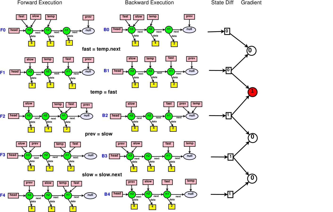
Figure 5: The forward and backward execution states of the program shown in Figure 4

5.2 Algorithm

We repeat the notations used for the reader’s convenience: $\mathcal{S}$ represents a state of a program with a set of variables $\sigma_{V}$ and a set of heap nodes $\sigma_{H}$ with fields $\sigma_{F}$ as $\mathcal{V}\times\mathcal{H}$; the state of the program variables, $\mathcal{V}$, is a map $\sigma_{V}\rightarrow\mathcal{D}$ and the program heap is represented by $\mathcal{H}$ as a map $\sigma_{H}\times\sigma_{F}\rightarrow\mathcal{D}$. The domain of possible values, $\mathcal{D}$, is $\mathcal{I}\cup\sigma_{H}$ where $\mathcal{I}$ is the set of integers. For simplicity, we constrain the discussions in this paper to only two data-types: integers and pointers. We use the function $\Upsilon(e)$ to fetch the type of a program entity; a program entity $e\in\mathcal{E}$ is either a variable $v\in\sigma_{V}$ or a field of a heap node $h\in\sigma_{H}\times\sigma_{F}$. Also, pointers can only point to heap nodes as we do not allow taking reference to variables.

5.2.1 Forward Execution

Let $\Delta$ denote the operational semantics in the forward execution.

$\Delta:State\times statement\to State$

The (repaired) program must satisfy the correctness criterion: $\Delta(\omega_{pre},stmt)$ = $\omega_{post}$

where $stmt$ is a program statement and $\omega_{pre}$, $\omega_{post}$ are the precondition (state before executing statement ‘‘stmt") and postcondition (state after executing statement ‘‘stmt").

Given a program trace of $n$ statements $[s_{0},s_{1},\dots,s_{n}]$, we define $\Delta_{i}$ as the transition function for the $i^{th}$ statement ($s_{i}$) in the trace. Subsequently, we denote $\Delta_{i,j}$ to denote the forward transition function for statements from statements $s_{i}$ to $s_{j}$.

$\Delta_{i,j}$ = $\Delta_{i}\circ\Delta_{i+1}\circ\Delta_{i+2}\circ\dots\circ\Delta_{j}$

In particular, a transition function for a complete trace of n statements can be written as:

$\Delta_{1,n}$ = $\Delta_{1}\circ\Delta_{2}\circ\Delta_{3}\circ\dots\circ\Delta_{n}$

Forward execution follows the forward semantics (Figure LABEL:fig:fwd_semantics). We illustrate forward execution via Figure 5: we use the getfld rule to execute $fast=temp.next$; the node pointed by fast is updated to n1 (state F1). We, then, use the asgn rule to execute $temp=fast$, which changes the node pointed by temp from n2 to n1(state F2). Then, we again use the asgn rule to update the value of prev to n3, followed by getfld rule, to revise value of slow to the node n2 (F3 and F4 respectively).

5.2.2 Backward Execution

We use $\nabla$ to denote the operational semantics for the backward execution.

$\nabla:State\times statement\to 2^{State}$

In this case, we may get a set of states instead of a single state (as the same state could be reached by multiple input states).

$\nabla(\omega_{post},stmt)$ = $\{\omega_{pre_{1}},\omega_{pre_{2}},\omega_{pre_{3}},\dots\}$

$\nabla_{n,0}(\omega_{post})$ = $\nabla_{n,n-1}\circ\nabla_{n-1,n-2}\circ\nabla_{n-2,n-3}\circ\dots\circ\nabla_{1,0}$ = $\{\Omega_{in1},\Omega_{in2},\dots\}$

⬇

1a = a->next;

2a = curr;

3if (curr != NULL){

4 b = b->next;

5 b = curr;

6 curr = curr->next;

7} \end{lstlisting}

8 \end{minipage}

9 \caption{Input program}

10 \label{fig:reverse_1}

11\end{subfigure}%

12 ~

13\begin{subfigure}[t]{0.55\textwidth}

14 \centering

15 \begin{minipage}{0.90\textwidth}

16 \begin{lstlisting}[language = C]

17(true) : a = a.next

18(true) : a = curr

19(true) : b0 = (curr != NULL)

20(b0) : b = b.next

21(b0) : b = curr

22(b0) : curr = curr.next

(a) IR of the program shown in Figure LABEL:fig:reverse_1

Figure 6: IR for a program with multiple statements in conditional block.

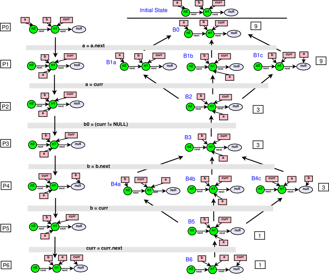
Figure 7: Forward and Backward execution of IR code shown in Figure 6(a)

We define the backward execution in Figure 7. Let us illustrate it using the program shown in Figure LABEL:fig:reverse_1 (and its IR in Figure 6(a)). This program has no bug, and we only use it for elucidation. Backward execution uses the rules described in Figure 8. P0 represents the program state before the start of the execution, and P6 shows the program state after all statements have been executed. We have copied the state P0 to Initial State and state P6 to B6 on the right-hand side for convenience. $N$ is the set of all nodes (including null) in the program at a particular program point. Starting from state B6, it uses getfld₁ rule, (because the LHS of statement $curr=curr\rightarrow next$ does not appear in any previous program statement) and this updates the value of curr to its value in the Initial State (node n1), as shown in state B5. We define two program statements as matching if their LHS writes to the same program variable or to a field of the same program variable. Now, since the LHS of statement $b=curr$ is same as LHS of previous statement $b=b\rightarrow next$, therefore we cannot read the value of b from the initial state. In this case, b is the variable to which both of these statements are writing. The value of b has changed (from that in initial state P0) due to the presence of a matching statement. Since we cannot be sure of the actual value of b at this program point, to perform backward execution, we assign all possible node values (including null) to b. We call this process ‘‘splitting of states". This is the use of asgn₂ rule and the set of possible states is B4(a), B4(b) and B4(c).

For backward executing $b=b.next$, Wolverine2 uses getfld₁ rule to update the value of b. This rule was used because, now, no previous program statement has the same LHS (b). Therefore, we update all the states (B4(a), B4(b) and B4(c)) with the value of b in the initial state (node n1) to give state B3. Although we maintain all the split states, we only show unique states in the figure. Next, the bassign rule is used, which performs no updates to the state (shown in state B2). Now, we will again have to split states as the LHS of statement $a=curr$ and $a=a\rightarrow next$ are the same. Wolverine2 uses the asgn₂ rule to assign all possible node values to a, and the obtained set of states are shown in B1(a), B1(b) and B1(c). Finally, the getfld₁ rule is used to revise the value of a, and this time, it can be read from the initial state (node n2); this state is labelled as B0. Note that, in this case, state B0 converges to the Initial State, showing that the program does not have a bug.

$$(\langle\mathcal{V}_{1},\mathcal{H}_{1}\rangle,x\mathrel{:}=y)\overset{\nabla}{\implies}\langle\mathcal{V}_{2},\mathcal{H}_{1}\rangle\lx@proof@logical@and\Upsilon(x)=\Upsilon(y)\mathcal{V}_{2}=\mathcal{V}_{1}[x\mapsto\mathcal{V}_{pre}(x)]{\\ }\textrm{x:=y is upward exposed}$$

$$(\langle\mathcal{V}_{1},\mathcal{H}_{1}\rangle,x\mathrel{:}=y)\overset{\nabla}{\implies}\langle\mathcal{V}_{2},\mathcal{H}_{1}\rangle\lx@proof@logical@and\Upsilon(x)=\Upsilon(y)\mathcal{V}_{2}=\mathcal{V}_{1}[x\mapsto n\ |\ n\ \overset{*}{\leftarrow}\ N]{\\ }\textrm{x:=y is not upward exposed}$$

$$(\langle\mathcal{V}_{1},\mathcal{H}_{1}\rangle,grd\text{ ? }stmt)\overset{\nabla}{\implies}\langle\mathcal{V}_{2},\mathcal{H}_{2}\rangle(\langle\mathcal{V}_{1},\mathcal{H}_{1}\rangle,\text{stmt})\overset{\nabla}{\implies}\langle\mathcal{V}_{2},\mathcal{H}_{2}\rangle$$

$$(\langle\mathcal{V}_{1},\mathcal{H}_{1}\rangle,command)\overset{\nabla}{\implies}\langle\mathcal{V}_{1},\mathcal{H}_{1}\rangle command\in\{band,bor,bassign,skip\}$$

Figure 8: Backward Semantics of our intermediate representation

5.2.3 Bug Localization Algorithm

We start our discussion about the algorithm by stating the following lemmas. Let $\Omega$ denote a set of states, while $\omega$ represents a single state.

Lemma 1

If $i^{th}$ statement is upward exposed then, $\Delta_{0,i-1}(\omega_{pre},P)[LHS(s_{i})]\ =\ \omega_{pre}[LHS(s_{i})]$.

Proof

Since $i^{th}$ statement is upward exposed, no other preceding statement or aliased variable can change the value of $LHS(s_{i})$, hence its value remains the same as in precondition ($\omega_{pre}$).

Lemma 2

If $i^{th}$ statement is downward exposed then, $\nabla_{n,i+1}(\omega_{post},P)[LHS(s_{i})]\ =\ \omega_{post}[LHS(s_{i})]$.

Proof

Since $i^{th}$ statement is downward exposed, no other succeeding statement or alias variable changes the value of $LHS(s_{i})$, hence its value remains the same as in postcondition ($\omega_{post}$) during backward execution. There has not been any splitting of states for $LHS(s_{i})$ before $i^{th}$ statement is backward traversed.

We provide our complete bug localization algorithm (Algorithm 2) for detecting suspicious program statements. Line 2 in Algorithm 2 is the forward trace, that is, the sequence of states obtained from the forward execution of the program. Line 3 is the backward trace, or the sequence of states obtained from backward execution; as we have seen, spitting can happen in the backward execution leading to several states at a program point (so $\Omega_{i}$ is a set of states). Since the splitting is uniform, we can count the number of children of a particular state in the backward trace by dividing the final number of states at the end of backward execution (denoted by M) and the number of states at that program point. This process gives a multiplying factor at each program point. Line 4 calculates the distance between the state in forward execution and the state(s) in backward execution, multiplied by the multiplying factor pertaining to that point. This operation is denoted by $\otimes$ in the algorithm. Each $\Gamma_{i}$ stores the result of this operation. Starting from the last program statement, if the pairwise difference of the $\Gamma_{i}$’s is non-zero (this is the gradient), the $i^{th}$ statement is added to the set of suspicious statements (Line 5-7), which is returned at the end (Line 9).

Let the number of states in ${\nabla(P,\Omega_{post},i)}$ be p and the number of states at the end of backward execution ${\nabla_{n,0}(P,\Omega_{post})}$ be M.

Let $\nabla_{n,i}=\Omega^{b}_{i}$ and $\Delta_{1,i}=\omega^{f}_{i}$. Then,

$$\Gamma_{i}=\omega^{f}_{i}\otimes\Omega^{b}_{i}=\frac{M}{|\Omega^{b}_{i}|}*(|\Omega^{b}_{i}[n]-\omega^{f}_{i}|+|\omega^{f}_{i}[n]-\Omega^{b}_{i}|)$$

In Figure 7, upon complete backward execution, we get a total of 9 states. The number of states at every program point is shown on the right-hand side (in the aligned box) Figure 7. The multiplying factor for a state can be determined by dividing 9 by its number of states.

$\Gamma_{1}$ at P1 is the sum of the difference between the nine states in backward execution (right side), out of which only three are shown (as others are duplicated). With the state in forward execution (left side) at P1, the sum of differences is 6.

We provide the theoretical analysis of this algorithm in the Appendix.

Input: $\phi::[\langle P,n,\Omega_{pre},\Omega_{post}\rangle]$

1 $SuspiciousSet=\{\}$

2 $[\omega^{f}_{0},\omega^{f}_{1},\omega^{f}_{2},\dots,\omega^{f}_{n}]\leftarrow[\mathcal{I},\Delta_{1,1},\Delta_{1,2},\dots\Delta_{1,n}](\omega_{pre}$, P)

3 $[\Omega^{b}_{0},\Omega^{b}_{1},\Omega^{b}_{2},\dots,\Omega^{b}_{n}]\leftarrow[\nabla_{n,1},\nabla_{n,2},\dots\nabla_{n,n},\mathcal{I}](\omega_{post}$, P)

4 $[\Gamma_{0},\Gamma_{1},\Gamma_{2},\dots,\Gamma_{n}]\leftarrow[\omega^{f}_{0},\omega^{f}_{1},\omega^{f}_{2},\dots,\omega^{f}_{n}]\otimes[\Omega^{b}_{0},\Omega^{b}_{1},\Omega^{b}_{2},\dots,\Omega^{b}_{n}]$

5 for $i\in\{1\dots n\}$ do

6       if $\Gamma_{i-1}\neq\Gamma_{i}$ then

7            $SuspiciousSet=SuspiciousSet\cup\{i\}$

8      

9 end for

10return SuspiciousSet

Algorithm 2 Pick suspicious statements

6 Advanced Debugging/Repair

In this section, we show how skilled engineer can employ the features in Wolverine2 for effective debug-repair sessions.

6.1 Specification Refinement

Wolverine2 is designed to model heap manipulations; however, Wolverine2 can use the concrete($\zeta$) statement in its intermediate representation as an abstraction of any statement $\zeta$ that it does not model. On hitting a concrete($\zeta$) statement, Wolverine2 uses gdb to concretely execute the statement and updates its symbolic state from the concrete states provided by gdb. Figure 10 shows an instance where we wrap the i=i+1 statement in an concrete execution; Wolverine2 translates this statement to a string of gdb commands, and the symbolic state is updated with the value of $i$ from the concrete state that gdb returns after executing the statement. Hence, although Wolverine2 is specifically targeted at heap manipulations, it can also be used to debug/repair programs containing other constructs as long as the bug is in heap manipulation statements. We refer to this technique of reconstructing the symbolic specification by running the statement concretely as specification refinement.

Specification refinement can be used in creative ways by skilled engineers. In Figure 10, the programmer decided to wrap a complete function call (foo()) within the concrete() construct, allowing Wolverine2 to reconstruct the effect of the function call via concrete execution without having to model it. This strategy can fetch significant speedups for repair: let us assume that, in Figure 1, the programmer uses her domain knowledge to localize the fault to Lines 6--8; she can pass this information to Wolverine2 by wrapping the other statements in the loop (lines 5,9) in concrete statements; this hint brings down the repair time on the full program on the complete execution from 6.0s to 1.5s, i.e., achieving a 4$\times$ speedup (on our machine). For this experiment, we turned off the fault localizer in Wolverine2. This is understandable as each instruction that is modeled can increase the search space exponentially.

6.2 Checkpoint-based Hopping

⬇

1void bar(){

2 struct node *current=NULL; int i;

3 current = head;

4 while (current != NULL){

5 concrete[i = foo();] //concrete stmt

6 current->data = i;

7 current = current->next;

8 }

9}

Figure 9: Refinement with concrete function calls

⬇

1struct node *head;

2void reverse(){

3 struct node *current, *temp1=NULL, *temp2=NULL;

4 current = head;

5 while (current != NULL){ // CheckPt 0

6 temp1 = current->prev;

7 temp2 = current->next;

8 current->prev = temp1; // FIX1: LHS = temp2;

9 current->next = temp2; // FIX2: LHS = temp1;

10 current = current->prev;

11 } // CheckPt 1; CheckPt 2; CheckPt 3

12 head = temp1->prev;

13}

14...

15int main(){

16 push(2); push(4); push(8); push(10);

17 reverse();

18}

Figure 10: Example for checkpoint-based hopping

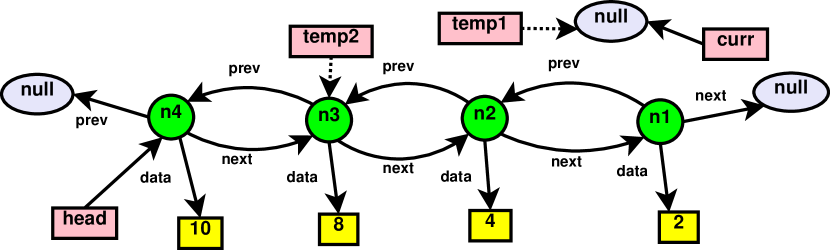
(a) At the end of first loop iteration
(before user changes)

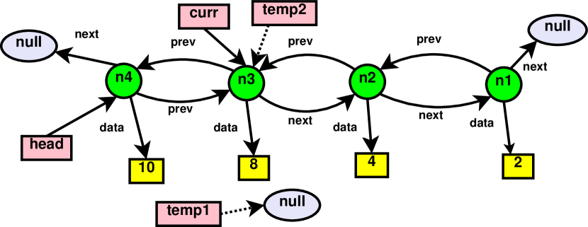
(b) At the end of first loop iteration
(after user changes)

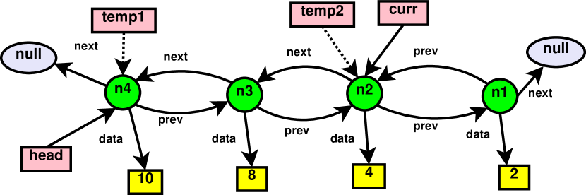
(c) At the end of second loop iteration
(after user changes)

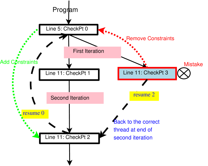
(d) Graph showing initial and final checkpoints for resume0 and resume2, and handling of the constraints for resume2.

Figure 11: Figures for checkpoint-based hopping example

This feature comes in handy when the programmer herself is not sure about the correctness of the expected specification she is asserting. For example, Figure 10 shows the code for reversal of a doubly-linked list, with bugs in two statements in the while loop (these bugs are different from the ones in Figure 1).

The programmer steps into the reverse() function after creating the doubly linked-list.

(Wolverine2) start Starting program... push(2) (Wolverine2) next; next; next; next;

push(4); …

reverse(); (Wolverine2) step

current = head; (Wolverine2) next

She executes the first statement in reverse() and then asserts the program state. Whenever the user asserts a state, Wolverine2 creates a checkpoint of this state at that program point; checkpointing memorizes important events during a debug run, allowing the user to resume a new direction of debugging from this location, if required (illustrated later). A Checkpoint ID, which keeps a count of the checkpoints (0 in this case), is returned. This ID can be used to resume debugging from this corresponding checkpoint/

while(current != NULL) (Wolverine2) spec Program states added -- Checkpoint 0 (Wolverine2) enter

She employs the next command to execute till the end of the loop.

temp1 = current->prev; (Wolverine2) next; next; next; next; next; … while(current != NULL)

The program state displayed to her is shown in Figure 11(a): due to the fact that the effect of Bug#1 and Bug#2 cancel out, she observes that the data-structure has not changed except the current pointer. Since she expected the reversal of the first node by the end of this loop iteration, she issues the desired changes and asserts the state (Checkpoint 1); the updated heap is shown in Figure 11(b).

(Wolverine2) change n4 -> prev n3 (Wolverine2) change current -> n3
while(current != NULL) (Wolverine2) spec Program states added -- Checkpoint 1

She now enters the loop for the second time.
(Wolverine2) enter while(current != NULL) …

At the end of this iteration, the user again finds an unexpected state and issues necessary changes to reverse the next node.

(Wolverine2) change current n2 (Wolverine2) change n3 -> prev n2 (Wolverine2) change n3 -> next n4

Satisfied with the updated state (shown in Figure 11(c)), she asserts it (Checkpoint 2).

while(current != NULL) (Wolverine2) spec Program states added -- Checkpoint 2

She, now, feels less convinced about her hypothesis regarding the correct run of the program and, thus, about the asserted program states and, therefore, decides to try out another direction of investigation. This would have required her to abandon the current session and spawn a new session; not only will it require her to resume debugging from the beginning, but she would also lose the current debugging session, preventing her from resuming in case she changes her mind again. Wolverine2 packages feature for such a scenario where a programmer may be interested in exploring multiples directions, allowing them to save and restore among these sessions at will. In this case, instead of exploring from the initial state, the programmer adds a checkpoint for the current state (Checkpoint 2) and returns to Checkpoint 0 by issuing resume 0.

while(current != NULL) (Wolverine2) resume 0 Program resumed at checkpoint 0

She executes through the first loop iteration in a similar manner (thus, the obtained state is the same as shown in Figure 11(a)). She issues the following changes to match her expectations and asserts the updated program state (Checkpoint 3).

(Wolverine2) change current n3 (Wolverine2) change n3 -> prev n4 (Wolverine2) change n3 -> next null
while(current != NULL) (Wolverine2) spec Program states added -- Checkpoint 3

To her surprise, the state shown to her remains unchanged after these modifications (barring the current pointer). She is now more confident that the states she had asserted in the previous session were correct and now wants to return to it. She issues resume 2.

Wolverine2 essentially maintains the constraints corresponding to the checkpointed states along with the different debugging states in a directed-acyclic graph; when the programmer resumes from checkpoint 2, Wolverine2 pops off all the constraints that were asserted till the first common ancestor (Checkpoint 0) of the current (Checkpoint 3) and the requested checkpointed state (Checkpoint 2) from the solver, and then, pushes the constraints till the resumed checkpoint (Checkpoint 2). They have been shown as red and green dotted lines, respectively, in Figure 11(d).

7 Experiments

Table 2: Our two sets of benchmarksGeeksForGeeks

Small benchmarks
B1	Reverse singly linked-list	B2	Reverse doubly linked-list
B3	Deletion from singly linked-list	B4	Creation of circular linked-list
B5	Sorted Insertion singly linked list	B6	Insertion in single linked list
B7	Swapping nodes singly linked list	B8	Splaytree Left Rotation
B9	Minimum in Binary Search Tree	B10	Find Length of singly linked list
B11	Print all nodes singly linked list	B12	Splitting of circular linked list
B13	AVL tree right rotation	B14	AVL tree left-right rotation
B15	AVL tree left rotation	B16	AVL tree right-left rotation
B17	Red-Black tree left rotate	B18	Red-Black tree right rotate
B19	Enqueue using linked-list	B20	Splaytree Right Rotated
Large benchmarks
L1	Delete middle of singly linked-list	L2	Remove dupilcate in singly linked-list
L3	Last node to first singly linked-list	L4	Intersection of two singly linked-list
L5	Split singly linked-list into two lists	L6	Value-based partition of singly linked-list
L7	Delete specific node in singly linked-list	L8	Splitting of circular linked-list
L9	Middle node as head singly linked-list	L10	Merge alternate nodes in singly linked-list
L11	Delete node of specific value in singly linked-list	L12	Splitting of doubly linked-list
L13	Pairwise swap of nodes in singly linked-list	L14	Rearranging singly linked-list
L15	Absolute sort of nodes in singly linked-list	L16	Quicksort of singly linked-list
L17	Delete specific node in doubly linked-list	L18	Sorted insertion in singly linked-list
L19	Remove duplicate nodes in doubly linked-list	L20	Constrained deletion in singly linked-list

We built Wolverine2 using the gdb Python bindingsgdbapi , the C-to-AST compiler uses pycparserpycparser , the visualization module uses igraphigraph to construct the box and arrow diagrams and the repair module uses the Z3z3 theorem prover to solve the SMT constraints. We conduct our experiments on an Intel(R) Xeon(R) CPU @ 2.00GHz machine with 32 GB RAM. To evaluate our implementation, we attempt to answer the following research questions:

RQ1.

Is our repair algorithm able to fix different types and combinations of bugs in a variety of data-structures?

RQ2.

Can our repair algorithm fix these bugs in a reasonable time?

RQ3.

How does our repair algorithm scale as the number of bugs is increased?

RQ4.

What is the accuracy of our localization algorithm with respect to other localization algorithms?

RQ5.

What is the impact of our algorithm (localization + repair) on the repair time of Wolverine2?

RQ6.

Is Wolverine2 capable of debugging/fixing real bugs?

We conduct our study on 40 heap manipulating programs (Table 2) from online sources GeeksForGeeks for a variety of data-structures like singly, doubly, and circular linked lists, AVL trees, Red-Black trees, Splay Trees, and Binary Search Trees.

Though there has been a large body of work on automated debugging and repair anagelicDebugging:2011 ; Angelix:2016 ; prophet:2016 ; genProg:2012 ; semfix:2013 ; Modi:2013 ; nguyen:2009 ; weimer:2009 ; weimer:2006 ; Loncaric:2018 ; Abhik:2016 ; Nguyen:2019 ; Ulysis ; Kolahal ; Gambit ; Pandey:2019 ; Bavishi2016b , these techniques cannot tackle repair over deep properties like functional correctness of heap data-structures. Our work is more in line with the following papers involving synthesis and repair of heap manipulating programs Singh:2011 ; similarbenchmark1 ; similarbenchmark2 ; Roy:2013 ; Garg:2015 ; similarbenchmark3 ; similarbenchmark12 or that involve functional correctness of student programs similarbenchmark4 ; similarbenchmark5 ; similarbenchmark6 ; similarbenchmark7 ; similarbenchmark8 ; similarbenchmark9 ; similarbenchmark10 ; similarbenchmark11 ; similarbenchmark13 . Hence, our collection of benchmarks are similar to the above contributions.

We divide our benchmarks into Small and Large benchmarks: the Large benchmarks involve more complex control-flow (nested conditions and complex boolean guards) and are about 3$\times$ larger than the Small programs (in terms of the number of IR instructions).

7.1 Experiments with Fault-Injection

We create buggy versions via an in-house fault injection engine that automatically injects bugs (at random), thereby eliminating possibilities of human bias. For each program, we control our fault-injection engine to introduce a given number of bugs. We characterize a buggy version by $\langle x,y\rangle$, implying that the program requires mutation of $x$ (randomly selected) program expressions and the insertion of $y$ newly synthesized program statements. The value of $x$ is determined by the number of mutations in the correct program. A mutation consists of replacing a program variable or the field of a variable with another variable or another field (randomly chosen from the program space) in a program statement or a guard. The value of $y$ is determined by the number of program statements the engine deletes from the correct program. Wolverine2 is unaware of the modifications and deletions when fed the modified program.

For the experiments, Wolverine2 makes ten attempts at repairing a program, each attempt followed by proof-directed search space widening; each attempt is run with a timeout of 30s. The experiment was conducted in the following manner:

1. We evaluate each benchmark (in Table 2) for four bug classes: Class1 ($\langle 1,0\rangle$), Class2($\langle 1,1\rangle$), Class3($\langle 2,0\rangle$) and Class4($\langle 2,1\rangle$);

2. For each benchmark $B_{i}$, at each bug configuration $\langle x,y\rangle$, we run our fault injection engine to create 40 buggy versions with x errors that require modification of an IR instruction and y errors that require insertion of a new statement;

3. Each of the above buggy programs is run twice to amortize the run time variability.

For RQ1 and RQ2, we use the 20 Small programs as these experiments involve only the repair tool (sans the localizer). Figure 12 shows the average time taken to repair a buggy configuration over the 20 buggy variants, which were themselves run twice (the reported time shows the average time taken for the successful repairs only). We report the time taken for our main algorithm (in Algorithm 1) and its variant AlgVar (discussed in the last paragraph in §4). Our primary algorithm performs quite well, fixing most of the repair instances in less than 5 seconds; understandably, the bug classes that require insertion of new instructions (Classes 2 and 4) take longer. There were about 1--4 widenings for bugs in class 1,2,3; the bugs in class 4 were more challenging, needing 2--6 widenings.

In terms of the success rate, our primary algorithm was able to repair all the buggy instances. However, Figure 12(c) shows the success rate for each bug configuration for AlgVar; the success rate is computed as the fraction of buggy instances (of the given buggy configuration) that could be repaired by Wolverine2 (in any of the two attempts).

The inferior performance of the variant of our main algorithm shows that the quality of the unsat cores is generally poor, while the performance of our primary algorithm demonstrates that even these unsat cores can be used creatively to design an excellent algorithm.

Figure 12(d) answers RQ3 by demonstrating the scalability of Wolverine2 with respect to the number of bugs on (randomly selected) five of our smaller benchmarks. We see that in most of the benchmarks, the time taken for repair grows somewhat linearly with the number of bugs, though (in theory), the search space grows exponentially. Also, one can see that more complex manipulations like left-rotation in a red-black tree (B17) are affected more as a larger number of bugs are introduced compared to simpler manipulations like inserting a node in a sorted linked list (B5).

The variance in the runtimes for the different buggy versions, even for those corresponding to the same buggy configuration, was found to be high. This is understandable as SMT solvers often find some instances much easier to solve than others, even when the size of the respective constraint systems is similar.

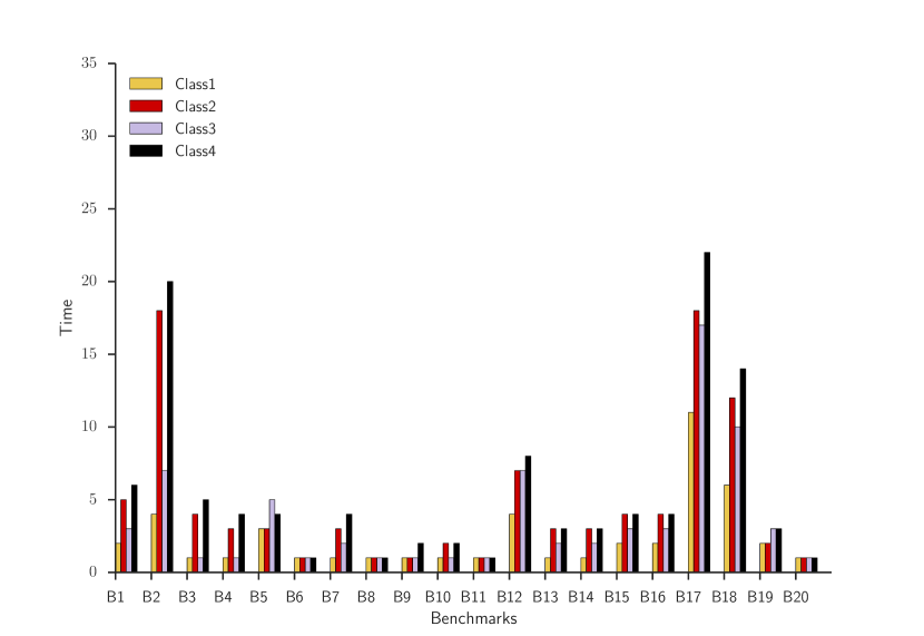
(a) Repair time for our primary algorithm

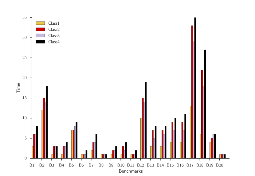
(b) Repair time for the variant (AlgVar)
of our primary algorithm

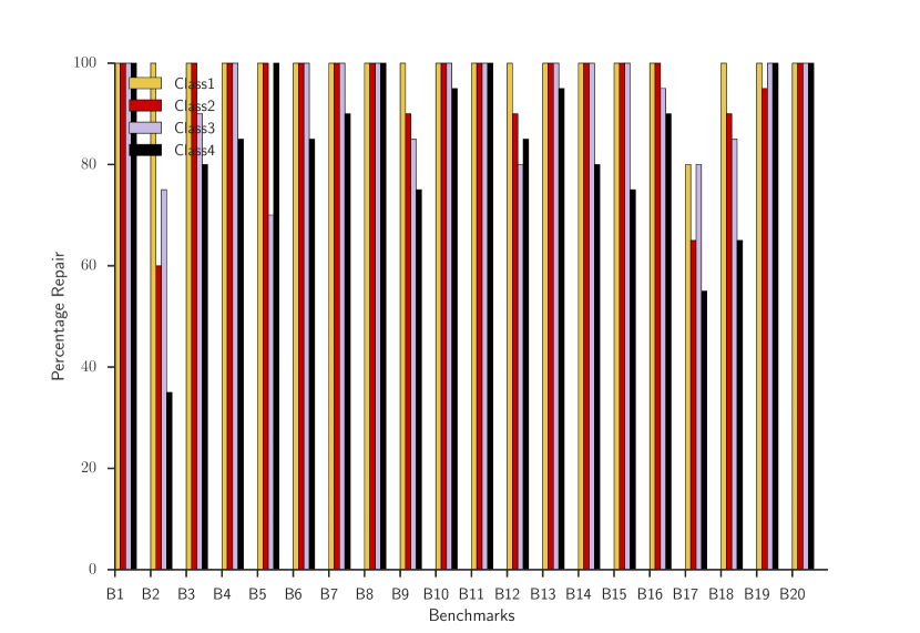
(c) Success rates for AlgVar; our primary
algorithm has 100% success rate in all cases.

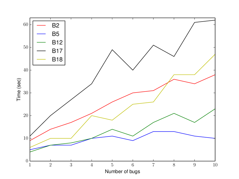
(d) Experiment showing the increase in repair time with increasing number of bugs

Figure 12: Performance of our repair algorithms

For RQ4, we compared our algorithm with the state-of-the-art bug localization algorithms we found in literature Sober:2005 ; liblit:2005 ; Tarantula:2005 ; Oichai:2009 . All these algorithms require the creation of test cases that differentiate between the correct and incorrect behavior of the program; our algorithm, on the other hand, does not require a test suite and localizes the bug using a single trace. To compare our algorithm against the existing algorithms, we developed a test generation engine for heap manipulating programs. We randomly selected 10 heap manipulating programs from our larger benchmarks (in Table 2). Bugs were injected using our fault injection engine. We created 20 versions of the program, each having a single bug for all the selected benchmarks (creating a total of 200 buggy programs). For each benchmark, Table 3 shows the average number of test cases generated, and the average statement and branch coverage produced by these test cases averaged over the 20 buggy versions.

To compare across benchmarks of differing sizes, we normalize the average rank of the buggy statement produced by these algorithms with the program size; hence, we report the developer effort, i.e., the percentage of the lines of code to be examined before the faulty line is encountered.

Figure 13 shows the line plot of the number of programs (out of 200) in which the average rank of the buggy statement produced by different algorithms was within a given effort threshold (% of program length on the x-axis). The plot shows that our algorithm is able to rank the ground truth repair in 150 of the 200 programs to within 10% of the program size, and all the 200 programs to 25% of the program size. On the other hand, the best performing metric among the other algorithms (Tarantula) is only able to rank 33 of the 200 programs to 25% of the program size.

Benchmark	# Tests	Line Coverage	Branch Coverage
B1	17.0	100.0	100.0
B2	61.0	89.0	89.0
B3	17.0	99.0	100.0
B4	335.0	100.0	100.0
B5	17.0	100.0	98.0
B6	121.0	100.0	100.0
B7	61.0	93.0	89.0
B8	17.0	98.0	99.0
B9	13.0	97.0	87.0
B10	17.0	93.0	96.0

Table 3: Coverage statistics of the tests generated for comparison with other bug localization techniques in  Figure 13

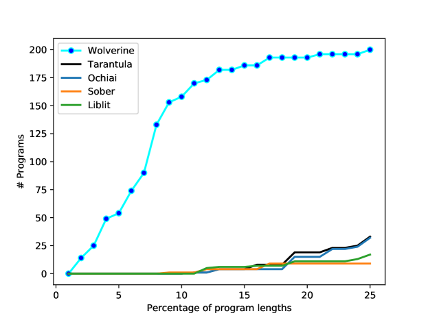
Figure 13: Comparison of ranking produced by Wolverine2 and other statistical bug localization algorithms

For RQ5, we choose all the 40 heap manipulating programs (in Table 2): for each benchmark, $B_{i}$, at each of the four configurations, we create 40 buggy versions. We compare our tool with two configurations of the repair tool (sans localization):

1. section-wise repair: when the user has some prior information about the bug and confines the repair tool’s search to only a section of the program (like the loop head, a loop body, etc.); a section can contain multiple nested control-flow statements but does not cross loop boundaries;

2. unconfined repair: the repair tool is unleashed on the whole program.

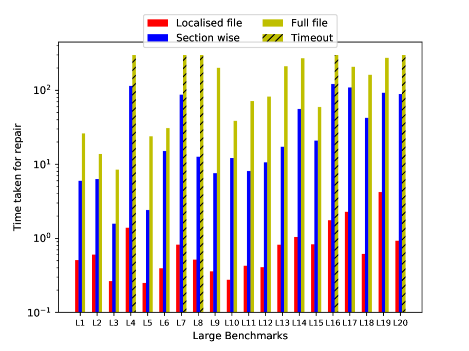
(a) Log scaled timing across localized, sectional-wise and unconfined repair (Class1)

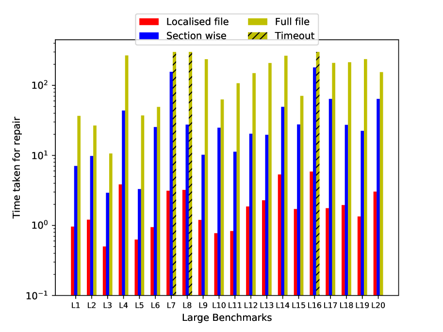
(b) Log scaled timing across localized, sectional-wise and unconfined repair (Class2)

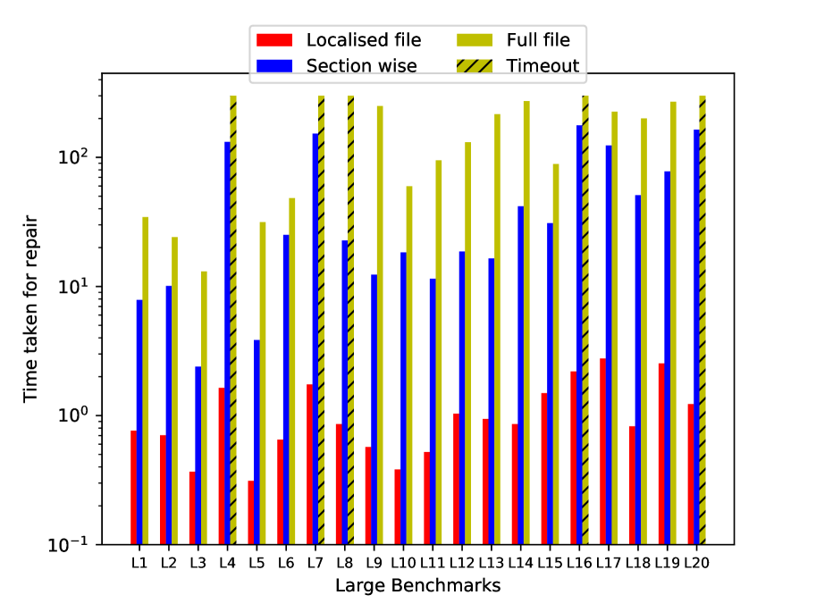
(c) Log scaled timing across localized, sectional-wise and unconfined repair (Class3)

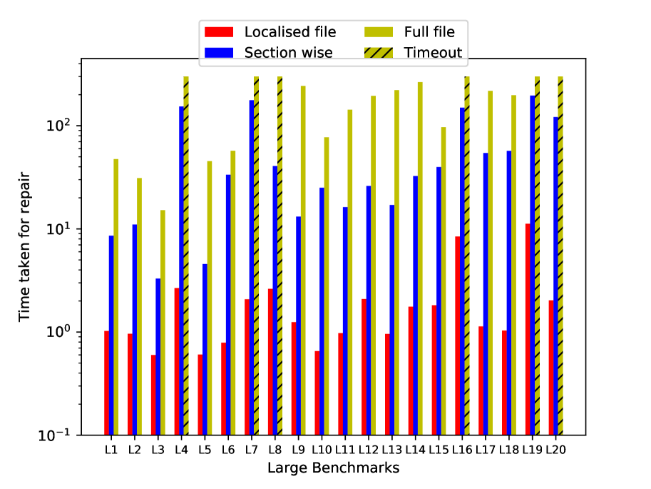
(d) Log scaled timing across localized, sectional-wise and unconfined repair (Class4)

Figure 14: Time comparison with and without localization (section-wise and unconfined) repair cases (second set of benchmarks)

Figure 14(a) compares the repair time (averaged over the 40 buggy versions for single bug configuration) required for Wolverine2 compared in three cases: (1) when localization is used, (2) when the bug is naively localized to a section of the code, and (3) when the bug localization is not used at all. The plot is in log scale. It clearly shows that using our bug localization algorithm reduces repair time by several orders of magnitude. On average over all benchmarks we were $50\times$ faster compared to the section-wise repair and $190\times$ (upto $779\times$ on some benchmarks) faster than in the unconfined repair setting.

Figure 14(b) shows the average repair time compared for the three cases for double bugs (two bugs in the program). Figure 14(c) shows the average repair time compared for the three cases for single bug and one insert slot configuration. Figure 14(d) shows the average repair time compared for the three cases for double bug and one insert slot configuration.

We show a summary of the average speedup results in  Table 4, both for the Small and Large instances (we do not provide plots for the smaller instances); understandably, localization benefits the Large benchmarks more than the Small benchmarks, illustrating the effectiveness of our localization algorithm in the repair of larger, more complex instances. For the programs that timed-out, we consider their runtimes as the timeout period (300s).

Table 4: Average speedups gained when compared to case of section-wise repair and case of unconfined repair. The numbers in the parenthesis show the maximum speedup obtained in respective classes for the case of unconfined repair.

Speed-ups for first set of benchmarks
Bug Configuration	Class1	Class2	Class3	Class4
Section-wise repair	14	4	10	8
Unconfined repair	39 (151)	12 (33)	31 (134)	22 (64)
Speed-ups for second set of benchmarks
Bug Configuration	Class1	Class2	Class3	Class4
Section-wise repair	50	20	54	28
Unconfined repair	190 (779)	80 (215)	170 (530)	86 (257)

7.2 Experiments with Student Submissions

In order to answer RQ6, we collected 247 buggy submissions from students corresponding to 5 programming problems on heap manipulations from an introductory programming course Prutor16 .

Table 5: Tool evaluation on student submissions

Id	Total	Fixed	Impl. Limit	Out of Scope	Vacuous
P1	47	30	2	8	7
P2	48	29	3	8	8
P3	48	36	0	5	7
P4	61	46	0	6	9
P5	43	25	0	4	14

We attempted repairing these submissions and categorized a submission into one of the following categories (shown in Table 5):

• Fixed: These are the cases where Wolverine2 could automatically fix the errors.

• Implementation Limitations: These are cases where, though our algorithm supports these repairs, the current state of our implementation could not support automatic repair.

• Out of scope: The bug in the submission did not occur in a heap-manipulating statement.

• Vacuous: In these submissions, the student, had hardly attempted the problem (i.e., the solution is almost empty).

Overall, we could automatically repair more than 80% of the submissions where the student has made some attempt at the problem (i.e., barring the vacuous cases).

8 Related Work

Our proof guided repair algorithm is inspired by a model-checking technique for concurrent programs---referred to as underapproximation widening Grumberg:2005 , that builds an underapproximate model of the program being verified by only allowing a specific set of thread interleavings by adding an underapproximation constraint that inhibit all others. If the verification instance finds a counterexample, a bug is found. If a proof is found which does not rely on the underapproximation constraint, the program is verified; else, it is an indication to relax the underapproximation constraint by allowing some more interleavings. Hence, the algorithm can find a proof from underapproximate models without needing to create abstractions. To the best of our knowledge, ours is the first attempt at adapting this idea for repair. In the case of repairs, performing a proof-guided search allows us to work on smaller underapproximated search spaces that are widened on demand, guided by the proof; at the same time, it allows us to prioritize among multiple repair strategies like insertion, deletion, and mutation. There have also been some attempts at using proof artifacts, like unsat cores, for distributing large verification problems Hydra . In the space of repairs, DirectFix DirectFix:2015 also builds a semantic model of a program but instead uses a MAXSAT solver to search for a repair. Invoking a MAXSAT solver is not only expensive, but a MAXSAT solver also does not allow prioritization among repair strategies. In DirectFix, it is not a problem as the tool only allows mutation of a statement for repair and does not insert new statements. Alternatively, one can use a weighted MAXSAT solver to prioritize repair actions, but it is prohibitively expensive; we are not aware of any repair algorithm that uses a weighted MAXSAT solver for repair.

Inspired by the success of Wolverine, there have been proposals at using proof-guided techniques for synthesis and repair: Gambit Gambit uses a proof-guided strategy for debugging concurrent programs under relaxed memory models. It also provides an interactive debugging environment, similar to Wolverine2, but focusses its debugging/repair attempts at concurrent programs, operating under varying memory models. Manthan Manthan1 ; Manthan2 uses a proof-guided approach to synthesis; instead of starting from a buggy program, its learns an initial version of the program from input-output examples. It, then, uses a similar repair engine as Wolverine and Wolverine2 to repair the candidate.

Zimmermann and Zeller Zimmermann:2001 introduce memory graphs to visualize the state of a running program, and Zeller used memory graphs in his popular Delta Debugging algorithms Zeller:2002b ; Zeller:2002 to localize faults. Our algorithm is also based on extracting these memory graphs from a concrete execution on gdb and employing its symbolic form for repair. The notion of concrete statement in Wolverine2 bears resemblance to the concolic testing tools Godefroid:2005 ; Sen:2005 .

Symbolic techniques groce:2006 ; ball:2003 ; liu:2010 ; jose:2011 ; BugAssist:2011 ; Bavishi:2016 ; Khurana:2017 ; Pandey:2019 ; Gambit build a symbolic model of a program and use a model-checker or a symbolic execution engine to ‘‘execute" the program; they classify a statement buggy based on the ‘‘distances" of faulty executions from the successful ones. Angelic Debugging anagelicDebugging:2011 , instead, uses a symbolic execution engine for fault localization by exploring alternate executions on a set of suspicious locations, while Angelix semfix:2013 ; Angelix:2016 fuses angelic debugging-style fault localization with a component-based synthesis Jha:2010 framework to automatically synthesize fixes. There have also been regression aware strategies to localize/repair bugs Bavishi:2016 . There have also been proposals to use statistical techniques Modi:2013 ; Sober:2005 ; liblit:2005 , evolutionary search genProg:2012 ; nguyen:2009 ; weimer:2009 ; weimer:2006 and probabilistic models prophet:2016 for program debugging. However, though quite effective for arithmetic programs, the above algorithms were not designed for debugging/repairing heap manipulations. There have been proposals that repair the state of a data-structure on-the-fly whenever any consistency check (from a set of checks provided by a user) is found to fail Demsky:2003 ; Juzi:2008 . However, our work is directed towards fixing the bug in the source code rather than in the state of the program, which makes this direction of solutions completely unrelated to our problem. In the space of functional programs, there has been a proposal Kneuss:2015 ; Feser:2015 to repair functional programs with unbounded data-types; however, such techniques are not applicable for debugging imperative programs. Finally, Wolverine2 uses a much lightweight technique for fault localization than expensive MAXSAT calls.

There has been some work in the space of synthesizing heap manipulations. The storyboard programming tool Singh:2011 uses abstract specifications provided by the user in three-valued logic to synthesize heap manipulations. As many users are averse to writing a formal specification, SYNBAD Roy:2013 allows the synthesis of programs from concrete examples; to amplify the user’s confidence in the program, it also includes a test-generation strategy on the synthesized program to guide refinement. SYNBAD inspires the intermediate representation of Wolverine2; Wolverine2 can also be extended with a test-generation strategy to validate the repair on a few more tests before exposing it to the programmer. SYNLIP Garg:2015 proposes a linear programming based synthesis strategy for heap manipulations. Feser et al. Feser:2015 propose techniques for synthesizing functional programs over recursive data structures. Wolverine2, on the other hand, attempts repairs; the primary difference between synthesis and repair is that, for a ‘‘good" repair, the tool must ensure that the suggested repair only makes ‘‘small" changes to the input program rather than providing a completely alternate solution. Other than synthesis of heap manipulations, program synthesis has seen success in many applications, from bit-manipulating programs Jha:2010 , bug synthesis BugSynthsis , parser synthesis Leung:2015 ; Singal:2018 and even differentially private mechanisms Kolahal . Fault localization techniques have seen both statistical and formal algorithms. Statistical debugging techniques Sober:2005 ; liblit:2005 ; Tarantula:2005 ; Oichai:2009 ; Ulysis ; Modi:2013 have been highly popular for large code-bases. These techniques essentially attempt to discover correlations between executions of parts of the program and its failure. However, though these techniques work quite well for large codebases, they are not suitable for somewhat smaller, but tricky programs, like heap manipulations. Our experiments (RQ4) demonstrate this and thus motivate different fault localization techniques for such applications. Moreover, these techniques essentially provide a ranking of the suspicious locations and hence are somewhat difficult to adopt with repair techniques. On the other hand, our localization algorithm provides a sound reduction in the repair space, thereby fitting quite naturally with the repair.

9 Discussion and Conclusion

We believe that tighter integration of dynamic analysis (enabled by a debugger) and static analysis (via symbolic techniques) can open new avenues for debugging tools. This work demonstrates that a concrete execution on a debugger to collect the potentially buggy execution and the user-intuitions on the desired fixes, fed to a bug localizer that contracts the repair space, and a proof-directed repair algorithm on the reduced search space, is capable of synthesizing repairs on non-trivial programs in a complex domain of heap-manipulations. We are interested in investigating more in this direction.

There exist threats to validity to our experimental results, in particular from the choice of the buggy programs and how the bugs were injected. We were careful to select a variety of data-structures and injected bugs via an automated fault injection engine to eliminate human bias; nevertheless, more extensive experiments can be conducted.

Appendix

Appendix A Theoretical Analysis of the Bug Localization Algorithm

Let $\mathcal{I}$ be the identity function that copies the $\omega_{pre}\text{ or }\omega_{post}$. Then,

$[\omega^{f}_{0},\omega^{f}_{1},\omega^{f}_{2},\dots,\omega^{f}_{n}]\leftarrow[\mathcal{I},\Delta_{1,1},\Delta_{1,2},\dots\Delta_{1,n}](\omega_{pre}$, P)
$[\Omega^{b}_{0},\Omega^{b}_{1},\Omega^{b}_{2},\dots,\Omega^{b}_{n}]\leftarrow[\nabla_{n,1},\nabla_{n,2},\dots\nabla_{n,n},\mathcal{I}](\omega_{post}$, P)
$[\Gamma_{0},\Gamma_{1},\Gamma_{2},\dots,\Gamma_{n}]\leftarrow[\omega^{f}_{0},\omega^{f}_{1},\omega^{f}_{2},\dots,\omega^{f}_{n}]\otimes[\Omega^{b}_{0},\Omega^{b}_{1},\Omega^{b}_{2},\dots,\Omega^{b}_{n}]$; $\Omega$ is a set of states while $\omega$ is a single state.

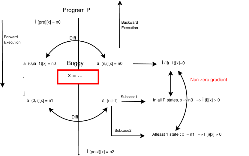
(a) Illustrations for case 1

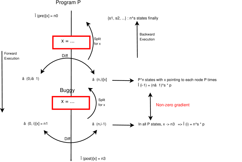
(b) Illustrations for case 3

Figure 15: Illustrations for the proof of theorem A.1

Theorem A.1

If a real bug is at location $i$, it implies that $i$ is in the suspicious set

Proof

Let $\hat{P}$ and $P$ denote the correct and buggy programs, respectively.

Assumption: Assume that in the trace $P_{n}$ (sequence of statements of length n), the $i^{th}$ statement has a real bug and $LHS(s_{i})$ be $x$. Let us define the correct execution as the forward execution states of $\hat{P}$ at each program point. Let $\Delta_{0,i}(\omega_{pre},\hat{P})[x]=\texttt{n1}$, $\Delta_{0,i}(\omega_{pre},P)[x]=\texttt{n2}$, $\omega_{post}[x]=\texttt{n3}$ and $\omega_{pre}[x]=\texttt{n0}$. Therefore, the number of nodes and points-to pairs in the datastructure, $\texttt{n}\geq 2$. [Assump1]

Case 1

The $i^{th}$ statement is upward exposed: this is illustrated in Figure 15(a).

1. $\Delta_{0,i-1}(\omega_{pre},P)$ = $\Delta_{0,i-1}(\omega_{pre},\hat{P})$ [Since the bug is in $i^{th}$ stmt]

2. $\nabla_{n,i}(\omega_{post},P)[x]=\omega_{pre}[x]$ [$asgn_{1}$ rule in Figure 8]

3. $\Delta_{0,i-1}(\omega_{pre},P)[x]=\omega_{pre}[x]$ [Lemma  1]

4. $\nabla_{n,i}(\omega_{post},P)[x]=\Delta_{0,i-1}(\omega_{pre},P)[x]$ [From 2 and 3]

5. $\Gamma_{i-1}[x]=0$ [Since $\Gamma_{i-1}=(\nabla_{n,i}-\Delta_{0,i-1})*(multiplyingfactor)$ and $\nabla_{n,i}-\Delta_{0,i-1}=0$]

6. Also since $i^{th}$ statement is upward exposed there is no previous splitting of states when this statement is backtracked. [Backward Semantics in Figure 8]

7. Without loss of generality, lets say there are already p backtracked states before $i^{th}$ statement is backtracked.

8. Subcase 1: There has not been any splitting for $x$ in the backward execution. Therefore for all the p states (in $\nabla_{n,i+1}$), $x$ points-to n3 [Stmt is both upward and downward exposed]

9. $\Gamma_{i}[x]=p*multiplyingfactor>0$ [From 8 and since $\Gamma_{i}=(\nabla_{n,i+1}-\Delta_{0,i})*(multiplyingfactor)$]

10. Subcase 2: There has been a previous splitting for $x$ in the backward execution. Therefore in atleast one of the p states, the value of $x\neq\texttt{n1}$. This is because splitting happens uniformly across all nodes and there are atleast 2 nodes in the data-structure. [Rules in Figure 8]

11. $\Gamma_{i}[x]>0$ [From 10]

12. Hence for loop at step 5 in Algorithm 2, since $\Gamma_{i-1}\neq\Gamma_{i},i^{th}$ statement will be added to suspicious set.

Case 2

The $i^{th}$ statement is sandwiched. We add all sandwiched statements to the suspicious set since the program loses all information regarding the correctness of such a statement.

Case 3

The $i^{th}$ statement is downward exposed and not upward exposed: this is illustrated in Figure 15(b).

1. There will be splitting of states when $i^{th}$ statement is backtracked. [$asgn_{2}$ rule in Figure 8]

2. Without loss of generality, lets say there are p backtracked states before $i^{th}$ statement is backward executed.

3. In all these p states, the value of variable $x=\texttt{n3}$. [Lemma  2]

4. Let there be s splits for $x$ until the full backtrack of the program.

5. The final number of states after backtracking is $n^{s}=M$, where $n$ is the number of nodes and points-to pairs [Rules in Figure 8]

6. Each of the p states contribute a difference of 1 in $\Gamma_{i}=p*\frac{n^{s}}{p}=n^{s}$ [$\Gamma_{i}=(\nabla_{n,i+1}-\Delta_{0,i})*(multiplyingfactor)$]

7. $\Gamma_{i-1}=\frac{n^{s}}{p*n}*(n-1)*p=n^{s}-n^{s-1}$ [Out of n nodes, 1 will match with a node in $\Delta_{0,i}(\omega_{pre},{P})$; uniform splitting]

8. $\Gamma_{i-1}-\Gamma_{i}=n^{s}-n^{s-1}-n^{s}\neq 0$, for $n>1$ [Since number of nodes and points-to pairs ¿ 1]

9. Hence, for the loop at step 5 in Algorithm 2, since $\Gamma_{i-1}\neq\Gamma_{i},i^{th}$ statement will be added to suspicious set.

In all cases, Algorithm 2 successfully catches the buggy statement.

Theorem A.2

If $C$ is the set of suspicious locations captured by Algorithm 2, then replacing all statements $s\notin C$ by $lhs=*$ maintains the ground truth repair in the proof-guided repair algorithm.

Proof

Any statement which depends on a buggy statement is also put in the suspicious set by our algorithm. This is natural because upon execution of the buggy statement, an incorrect state is achieved, and any statements which further depend on this state would be buggy with respect to the ground truth state. Hence, we can slice away the statement from repair by making them non-deterministic.

References

- [1] igraph -- the network analysis package. http://igraph.org/python/. Online; accessed 24 January 2017.
- [2] Rui Abreu, Peter Zoeteweij, Rob Golsteijn, and Arjan J. C. van Gemund. A practical evaluation of spectrum-based fault localization. J. Syst. Softw., 82(11), November 2009.
- [3] Thomas Ball, Mayur Naik, and Sriram K. Rajamani. From Symptom to Cause: Localizing Errors in Counterexample Traces. In Proceedings of the 30th ACM SIGPLAN-SIGACT Symposium on Principles of Programming Languages, POPL ’03, New York, NY, USA, 2003. ACM.
- [4] Rohan Bavishi, Awanish Pandey, and Subhajit Roy. Regression aware debugging for mobile applications. In Mobile! 2016: Proceedings of the 1st International Workshop on Mobile Development (Invited Paper), Mobile! 2016, page 21–22, New York, NY, USA, 2016. Association for Computing Machinery.
- [5] Rohan Bavishi, Awanish Pandey, and Subhajit Roy. To be precise: Regression aware debugging. In Proceedings of the 2016 ACM SIGPLAN International Conference on Object-Oriented Programming, Systems, Languages, and Applications, OOPSLA 2016, New York, NY, USA, 2016. ACM.
- [6] Eli Bendersky. Pycparser: C parser in Python. https://pypi.python.org/pypi/pycparser. Online; accessed 24 January 2017.
- [7] Sahil Bhatia, Pushmeet Kohli, and Rishabh Singh. Neuro-symbolic program corrector for introductory programming assignments. In Proceedings of the 40th International Conference on Software Engineering, ICSE ’18, New York, NY, USA, 2018. Association for Computing Machinery.
- [8] Satish Chandra, Emina Torlak, Shaon Barman, and Rastislav Bodik. Angelic Debugging. In Proceedings of the 33rd International Conference on Software Engineering, ICSE ’11, New York, NY, USA, 2011. ACM.
- [9] Prantik Chatterjee, Abhijit Chatterjee, Jose Campos, Rui Abreu, and Subhajit Roy. Diagnosing software faults using multiverse analysis. In Christian Bessiere, editor, Proceedings of the Twenty-Ninth International Joint Conference on Artificial Intelligence, IJCAI-20, pages 1629--1635. International Joint Conferences on Artificial Intelligence Organization, 7 2020. Main track.
- [10] Prantik Chatterjee, Subhajit Roy, Bui Phi Diep, and Akash Lal. Distributed bounded model checking. In FMCAD, July 2020.
- [11] Rajdeep Das, Umair Z. Ahmed, Amey Karkare, and Sumit Gulwani. Prutor: A system for tutoring CS1 and collecting student programs for analysis. CoRR, abs/1608.03828, 2016.
- [12] Leonardo De Moura and Nikolaj Bjørner. Z3: An efficient smt solver. In Proceedings of the Theory and Practice of Software, 14th International Conference on Tools and Algorithms for the Construction and Analysis of Systems, page 337–340, Berlin, Heidelberg, 2008. Springer-Verlag.
- [13] Brian Demsky and Martin Rinard. Automatic detection and repair of errors in data structures. In Proceedings of the 18th Annual ACM SIGPLAN Conference on Object-oriented Programing, Systems, Languages, and Applications, OOPSLA ’03, New York, NY, USA, 2003. ACM.
- [14] Bassem Elkarablieh and Sarfraz Khurshid. Juzi: A tool for repairing complex data structures. In Proceedings of the 30th International Conference on Software Engineering, ICSE ’08, New York, NY, USA, 2008. ACM.
- [15] John K. Feser, Swarat Chaudhuri, and Isil Dillig. Synthesizing data structure transformations from input-output examples. In Proceedings of the 36th ACM SIGPLAN Conference on Programming Language Design and Implementation, PLDI ’15, New York, NY, USA, 2015. ACM.
- [16] Geeks for Geeks. Data structures. http://www.geeksforgeeks.org/data-structures/. Online; accessed 24 January 2017.
- [17] Free Software Foundation. GDB Python API. https://sourceware.org/gdb/onlinedocs/gdb/Python-API.html. Online; accessed 25 January 2017.
- [18] Free Software Foundation. GDB: The GNU Project Debugger. https://sourceware.org/gdb/. Online; accessed 24 January 2017.
- [19] Anshul Garg and Subhajit Roy. Synthesizing heap manipulations via integer linear programming. In Sandrine Blazy and Thomas Jensen, editors, Static Analysis, SAS 2015. Proceedings. Springer Berlin Heidelberg, Berlin, Heidelberg, 2015.
- [20] Patrice Godefroid, Nils Klarlund, and Koushik Sen. Dart: Directed automated random testing. In Proceedings of the 2005 ACM SIGPLAN Conference on Programming Language Design and Implementation, PLDI ’05, New York, NY, USA, 2005. ACM.
- [21] Priyanka Golia, Subhajit Roy, and Kuldeep S. Meel. Manthan: A data-driven approach for boolean function synthesis. In Shuvendu K. Lahiri and Chao Wang, editors, Computer Aided Verification (CAV), pages 611--633, Cham, 2020. Springer International Publishing.
- [22] Priyanka Golia, Subhajit Roy, Friedrich Slivovsky, and Kuldeep S. Meel. Engineering an efficient boolean functional synthesis engine. In ICCAD, 2021.
- [23] Alex Groce, Sagar Chaki, Daniel Kroening, and Ofer Strichman. Error Explanation with Distance Metrics. Int. J. Softw. Tools Technol. Transf., June 2006.
- [24] Orna Grumberg, Flavio Lerda, Ofer Strichman, and Michael Theobald. Proof-guided underapproximation-widening for multi-process systems. In Proceedings of the 32Nd ACM SIGPLAN-SIGACT Symposium on Principles of Programming Languages, POPL ’05, New York, NY, USA, 2005. ACM.
- [25] Sumit Gulwani, Ivan Radiček, and Florian Zuleger. Automated clustering and program repair for introductory programming assignments. In Proceedings of the 39th ACM SIGPLAN Conference on Programming Language Design and Implementation, PLDI 2018, page 465–480, New York, NY, USA, 2018. Association for Computing Machinery.
- [26] Philip J. Guo. Online python tutor: Embeddable web-based program visualization for cs education. In Proceeding of the 44th ACM Technical Symposium on Computer Science Education, SIGCSE ’13, New York, NY, USA, 2013. ACM.
- [27] Rahul Gupta, Soham Pal, Aditya Kanade, and Shirish Shevade. Deepfix: Fixing common c language errors by deep learning. In Proceedings of the Thirty-First AAAI Conference on Artificial Intelligence, AAAI’17, page 1345–1351. AAAI Press, 2017.
- [28] C. A. R. Hoare. An axiomatic basis for computer programming. Commun. ACM, 12(10), October 1969.
- [29] Qinheping Hu, Roopsha Samanta, Rishabh Singh, and Loris D’Antoni. Direct Manipulation for Imperative Programs, pages 347--367. Springer International Publishing, 10 2019.
- [30] Yang Hu, Umair Z. Ahmed, Sergey Mechtaev, Ben Leong, and Abhik Roychoudhury. Re-Factoring Based Program Repair Applied to Programming Assignments, page 388–398. ASE ’19. IEEE Press, 2019.
- [31] Susmit Jha, Sumit Gulwani, Sanjit A. Seshia, and Ashish Tiwari. Oracle-guided component-based program synthesis. In Proceedings of the 32Nd ACM/IEEE International Conference on Software Engineering - Volume 1, ICSE ’10, New York, NY, USA, 2010. ACM.
- [32] James A. Jones and Mary Jean Harrold. Empirical evaluation of the tarantula automatic fault-localization technique. In Proceedings of the 20th IEEE/ACM International Conference on Automated Software Engineering, ASE ’05, New York, NY, USA, 2005. ACM.
- [33] Manu Jose and Rupak Majumdar. Bug-Assist: Assisting Fault Localization in ANSI-C Programs. In Proceedings of the 23rd International Conference on Computer Aided Verification, CAV’11, Berlin, Heidelberg, 2011. Springer-Verlag.
- [34] Manu Jose and Rupak Majumdar. Cause Clue Clauses: Error Localization Using Maximum Satisfiability. In Proceedings of the 32nd ACM SIGPLAN Conference on Programming Language Design and Implementation, PLDI ’11, New York, NY, USA, 2011. ACM.
- [35] Etienne Kneuss, Manos Koukoutos, and Viktor Kuncak. Deductive program repair. In CAV, 2015.
- [36] Claire Le Goues, ThanhVu Nguyen, Stephanie Forrest, and Westley Weimer. GenProg: A Generic Method for Automatic Software Repair. IEEE Trans. Softw. Eng., 38, January 2012.
- [37] Alan Leung, John Sarracino, and Sorin Lerner. Interactive parser synthesis by example. SIGPLAN Not., 50(6):565–574, June 2015.
- [38] Ben Liblit, Mayur Naik, Alice X. Zheng, Alex Aiken, and Michael I. Jordan. Scalable Statistical Bug Isolation. In Proceedings of the 2005 ACM SIGPLAN Conference on Programming Language Design and Implementation, PLDI ’05, New York, NY, USA, 2005. ACM.
- [39] Chao Liu, Xifeng Yan, Long Fei, Jiawei Han, and Samuel P. Midkiff. Sober: Statistical model-based bug localization. In ESEC/FSE-13, New York, NY, USA, 2005. ACM.
- [40] Yongmei Liu and Bing Li. Automated Program Debugging via Multiple Predicate Switching. In Proceedings of the Twenty-Fourth AAAI Conference on Artificial Intelligence, AAAI’10. AAAI Press, 2010.
- [41] Calvin Loncaric, Michael D. Ernst, and Emina Torlak. Generalized data structure synthesis. In Proceedings of the 40th International Conference on Software Engineering, ICSE ’18, page 958–968, New York, NY, USA, 2018. Association for Computing Machinery.
- [42] Fan Long and Martin Rinard. Automatic patch generation by learning correct code. In Proceedings of the 43rd Annual ACM SIGPLAN-SIGACT Symposium on Principles of Programming Languages, POPL ’16, New York, NY, USA, 2016. ACM.
- [43] M. Z. Malik, J. H. Siddiqui, and S. Khurshid. Constraint-based program debugging using data structure repair. In 2011 Fourth IEEE International Conference on Software Testing, Verification and Validation, March 2011.
- [44] Muhammad Zubair Malik, Khalid Ghori, Bassem Elkarablieh, and Sarfraz Khurshid. A case for automated debugging using data structure repair. In Proceedings of the 2009 IEEE/ACM International Conference on Automated Software Engineering, ASE ’09, USA, 2009. IEEE Computer Society.
- [45] Sergey Mechtaev, Jooyong Yi, and Abhik Roychoudhury. DirectFix: Looking for Simple Program Repairs. In Proceedings of the 37th International Conference on Software Engineering - Volume 1, ICSE ’15, pages 448--458, Piscataway, NJ, USA, 2015.
- [46] Sergey Mechtaev, Jooyong Yi, and Abhik Roychoudhury. Angelix: Scalable multiline program patch synthesis via symbolic analysis. In Proceedings of the 38th International Conference on Software Engineering, ICSE ’16, New York, NY, USA, 2016. ACM.
- [47] Varun Modi, Subhajit Roy, and Sanjeev K. Aggarwal. Exploring Program Phases for Statistical Bug Localization. In Proceedings of the 11th ACM SIGPLAN-SIGSOFT Workshop on Program Analysis for Software Tools and Engineering, PASTE ’13, New York, NY, USA, 2013. ACM.
- [48] Hoang Duong Thien Nguyen, Dawei Qi, Abhik Roychoudhury, and Satish Chandra. SemFix: Program Repair via Semantic Analysis. In Proceedings of the 2013 International Conference on Software Engineering, ICSE ’13, Piscataway, NJ, USA, 2013. IEEE Press.
- [49] Thanh-Toan Nguyen, Quang-Trung Ta, and Wei-Ngan Chin. Automatic program repair using formal verification and expression templates. In VMCAI, 2019.
- [50] ThanhVu Nguyen, Westley Weimer, Claire Le Goues, and Stephanie Forrest. Using execution paths to evolve software patches. In Software Testing, Verification and Validation Workshops, 2009. ICSTW’09. International Conference on, pages 152--153. IEEE, 2009.
- [51] Awanish Pandey, Phani Raj Goutham Kotcharlakota, and Subhajit Roy. Deferred concretization in symbolic execution via fuzzing. In Proceedings of the 28th ACM SIGSOFT International Symposium on Software Testing and Analysis, ISSTA 2019, page 228–238, New York, NY, USA, 2019. Association for Computing Machinery.
- [52] Van-Thuan Pham, Sakaar Khurana, Subhajit Roy, and Abhik Roychoudhury. Bucketing failing tests via symbolic analysis. In Marieke Huisman and Julia Rubin, editors, Fundamental Approaches to Software Engineering, pages 43--59, Berlin, Heidelberg, 2017. Springer Berlin Heidelberg.
- [53] Nadia Polikarpova and Ilya Sergey. Structuring the synthesis of heap-manipulating programs. Proc. ACM Program. Lang., January 2019.
- [54] Yewen Pu, Karthik Narasimhan, Armando Solar-Lezama, and Regina Barzilay. Sk_p: A neural program corrector for moocs. In Companion Proceedings of the 2016 ACM SIGPLAN International Conference on Systems, Programming, Languages and Applications: Software for Humanity, SPLASH Companion 2016, page 39–40, New York, NY, USA, 2016. Association for Computing Machinery.
- [55] Reudismam Rolim, Gustavo Soares, Loris D’Antoni, Oleksandr Polozov, Sumit Gulwani, Rohit Gheyi, Ryo Suzuki, and Björn Hartmann. Learning syntactic program transformations from examples. In Proceedings of the 39th International Conference on Software Engineering, ICSE ’17. IEEE Press, 2017.
- [56] S. Roy, J. Hsu, and A. Albarghouthi. Learning differentially private mechanisms. In 2021 2021 IEEE Symposium on Security and Privacy (SP), pages 852--865, Los Alamitos, CA, USA, May 2021. IEEE Computer Society.
- [57] Subhajit Roy. From concrete examples to heap manipulating programs. In Francesco Logozzo and Manuel Fähndrich, editors, Static Analysis: 20th International Symposium, SAS 2013, Seattle, WA, USA, June 20-22, 2013. Proceedings. Springer Berlin Heidelberg, Berlin, Heidelberg, 2013.
- [58] Subhajit Roy, Awanish Pandey, Brendan Dolan-Gavitt, and Yu Hu. Bug synthesis: Challenging bug-finding tools with deep faults. In Proceedings of the 2018 26th ACM Joint Meeting on European Software Engineering Conference and Symposium on the Foundations of Software Engineering, ESEC/FSE 2018, page 224–234, New York, NY, USA, 2018. Association for Computing Machinery.
- [59] Koushik Sen, Darko Marinov, and Gul Agha. CUTE: A Concolic Unit Testing Engine for C. In ESEC/FSE-13, New York, NY, USA, 2005. ACM.
- [60] Dhruv Singal, Palak Agarwal, Saket Jhunjhunwala, and Subhajit Roy. Parse condition: Symbolic encoding of ll(1) parsing. In Gilles Barthe, Geoff Sutcliffe, and Margus Veanes, editors, LPAR-22. 22nd International Conference on Logic for Programming, Artificial Intelligence and Reasoning, volume 57 of EPiC Series in Computing, pages 637--655. EasyChair, 2018.
- [61] Rishabh Singh, Sumit Gulwani, and Armando Solar-Lezama. Automated feedback generation for introductory programming assignments. In Proceedings of the 34th ACM SIGPLAN Conference on Programming Language Design and Implementation, PLDI ’13, New York, NY, USA, 2013. Association for Computing Machinery.
- [62] Rishabh Singh and Armando Solar-Lezama. Synthesizing data structure manipulations from storyboards. In Proceedings of the 19th ACM SIGSOFT Symposium and the 13th European Conference on Foundations of Software Engineering, ESEC/FSE ’11, New York, NY, USA, 2011. ACM.
- [63] Shin Hwei Tan, Hiroaki Yoshida, Mukul R. Prasad, and Abhik Roychoudhury. Anti-patterns in search-based program repair. In Proceedings of the 2016 24th ACM SIGSOFT International Symposium on Foundations of Software Engineering, FSE 2016, page 727–738, New York, NY, USA, 2016. Association for Computing Machinery.
- [64] Aakanksha Verma, Pankaj Kumar Kalita, Awanish Pandey, and Subhajit Roy. Interactive debugging of concurrent programs under relaxed memory models. In Proceedings of the 18th ACM/IEEE International Symposium on Code Generation and Optimization, CGO 2020, page 68–80, New York, NY, USA, 2020. Association for Computing Machinery.
- [65] Sahil Verma and Subhajit Roy. Synergistic debug-repair of heap manipulations. In Proceedings of the 2017 11th Joint Meeting on Foundations of Software Engineering, ESEC/FSE 2017, New York, NY, USA, 2017. ACM.
- [66] Ke Wang, Rishabh Singh, and Zhendong Su. Dynamic neural program embedding for program repair. ArXiv, abs/1711.07163, 2017.
- [67] Ke Wang, Rishabh Singh, and Zhendong Su. Search, align, and repair: Data-driven feedback generation for introductory programming exercises. In Proceedings of the 39th ACM SIGPLAN Conference on Programming Language Design and Implementation, PLDI 2018, page 481–495, New York, NY, USA, 2018. Association for Computing Machinery.
- [68] Westley Weimer. Patches As Better Bug Reports. In Proceedings of the 5th International Conference on Generative Programming and Component Engineering, GPCE ’06, New York, NY, USA, 2006. ACM.
- [69] Westley Weimer, ThanhVu Nguyen, Claire Le Goues, and Stephanie Forrest. Automatically Finding Patches Using Genetic Programming. In Proceedings of the 31st International Conference on Software Engineering, ICSE ’09, Washington, DC, USA, 2009. IEEE Computer Society.
- [70] Andreas Zeller. Isolating cause-effect chains from computer programs. In Proceedings of the 10th ACM SIGSOFT Symposium on Foundations of Software Engineering, SIGSOFT ’02/FSE-10, New York, NY, USA, 2002. ACM.
- [71] Andreas Zeller and Ralf Hildebrandt. Simplifying and isolating failure-inducing input. IEEE Trans. Softw. Eng., 28(2), 2002.
- [72] Thomas Zimmermann and Andreas Zeller. Visualizing memory graphs. In Revised Lectures on Software Visualization, International Seminar, London, UK, UK, 2002. Springer-Verlag.