Positive definiteness of real quadratic forms resulting from the variable-step approximation of convolution operators

Abstract

The positive definiteness of real quadratic forms with convolution structures plays an important role in stability analysis for time-stepping schemes for nonlocal operators. In this work, we present a novel analysis tool to handle discrete convolution kernels resulting from variable-step approximations for convolution operators. More precisely, for a class of discrete convolution kernels relevant to variable-step time discretizations, we show that the associated quadratic form is positive definite under some easy-to-check algebraic conditions. Our proof is based on an elementary constructing strategy using the properties of discrete orthogonal convolution kernels and complementary convolution kernels. To the best of our knowledge, this is the first general result on simple algebraic conditions for the positive definiteness of variable-step discrete convolution kernels. Using the unified theory, the stability for some simple non-uniform time-stepping schemes can be obtained in a straightforward way.

Keywords: discrete convolution kernels, positive definiteness, variable time-stepping, orthogonal convolution kernels, complementary convolution kernels

1 Introduction

In stability and convergence analysis of time-stepping schemes for integro-differential equations or time-fractional partial differential equations (see e.g.[1, 3, 12, 7, 16, 20]), we usually resort to the positive (semi-)definite property of the real quadratic form with convolution structure

$$\sum_{k=1}^{n}w_{k}\sum_{j=1}^{k}a_{k-j}w_{j}\quad\text{for any sequence $\{w_{1},w_{2},\cdots,w_{n}\}$,}$$ (1.1)

where the real sequence $\{a_{0},a_{1},\cdots,a_{n},\cdots\}$ is generated by a time approximation with the uniform time-step of certain convolution integrals such as the Riemann-Liouville fractional integrals and the Caputo fractional derivatives.

For uniform time-stepping approximations, the semi-positive definiteness of the above real quadratic form can be verified by applying a classical result due to Toeplitz and Carathéodory [4, p.18]. More precisely, if $\{a_{0},a_{1},\cdots,a_{n},\cdots\}$ is a sequence of real numbers such that

$$\hat{a}(z)=\sum_{k=0}^{\infty}a_{n}z^{k}\;\;\text{is analytic in the open unit disk $\mathcal{D}_{z}:=\{z\in\mathbb{C}:\left|z\right|<1\}$,}$$ (1.2)

then the corresponding real quadratic form is positive semi-definite if and only if

$$\mathrm{Re}\left[\hat{a}(z)\right]\geq 0\qquad\text{for any $z\in\mathcal{D}_{z}$.}$$ (1.3)

This result was widely used in numerical analysis of integro-differential equations, see e.g. [7, 14, 15, 16, 20].

In analyzing finite difference schemes for nonlinear integro-differential equations, López-Marcos [13, Proposition 5.2] presented a corollary of the above result with the following sufficient conditions for the real sequence $\{a_{0},a_{1},\cdots,a_{n},\cdots\}:$

$$a_{j}\geq 0,\quad a_{j-1}\geq a_{j},\quad a_{j-1}-a_{j}\geq a_{j}-a_{j+1}.$$ (1.4)

Notice that the above criterions are rather simple and easy-to-check. Actually, it has been shown to be powerful in stability and convergence analysis of uniform time-stepping approximations for integro-differential and time-fractional differential problems, see e.g., [2, 5, 22, 23].

However, in most practical applications, one may need to use nonuniform/variable time-stepping schemes. This is the case when one wants to capture the multi-scale behaviors in time, and/or one needs to handle solution singularities in time. In these situations, it is natural to investigate (semi-)positive definiteness of the following real quadratic form with convolution structure:

$$\sum_{k=1}^{n}w_{k}\sum_{j=1}^{k}a^{(k)}_{k-j}w_{j}\quad\text{for any sequence $\{w_{1},w_{2},\cdots,w_{n}\}$,}$$ (1.5)

where the associated (variable) discrete convolution kernels $\big{\{}a^{(n)}_{n-k}\big{\}}_{k=1}^{n}$ may be resulted from variable time-stepping approximations of the Caputo fractional derivative and Riemann–Liouville (convolution) integrals, see e.g., [6, 5, 8, 9, 10, 18, 19, 17]. Here the superscript $(n)$ represents the discrete time-level $t_{n}$ and the value of $a^{(n)}_{j}$ may vary at different time levels $t_{n}.$

It is noted that the extension of (1.2)-(1.3) or (1.4) to nonuniform time-stepping schemes is by no means trivial. In other words, one can not apply the criterions in [4, 13] to examine the positive definiteness of the quadratic form (1.5). We also remark that one may consider the so-called positive-semidefinite-preserving approach [6, 17, 18, 19] to deal with the positive definiteness of (1.5) as the associated discrete convolution kernels are discrete analogy of the positive definite continuous kernels. However, these specially designed discrete kernels are of very special form and the corresponding theory lacks application generality.

The aim of this work is to present some sufficient and easy-to-check criterions on a wide class of discrete convolution kernels $\big{\{}a^{(n)}_{n-k}\big{\}}_{k=1}^{n}$ to ensure the semi-positive definiteness of (1.5). For notation simplicity, we shall simply use $\mathcal{B}^{(n)}_{n-k}$ to represent a set of discrete convolution kernels $\big{\{}\mathcal{B}^{(n)}_{n-k}\big{\}}_{k=1}^{n}$ or $\big{\{}\mathcal{B}^{(n)}_{0},\mathcal{B}^{(n)}_{1},\cdots,\mathcal{B}^{(n)}_{n-1}\big{\}}.$ We say that the discrete convolution kernels $\mathcal{B}^{(n)}_{n-k}$ are positive (semi-)definite if the associated real quadratic form is positive (semi-)definite.

We now state our main theorem as follows.

Theorem 1.1.

For fixed $n\geq 2$, the discrete convolution kernels $a^{(n)}_{n-k}$ are positive definite if the following conditions are satisfied

$${\bf C1.}\qquad a^{(n)}_{j}>0 \mbox{for}\;\;0\leq j\leq n-1;$$

$${\bf C2.}\qquad a^{(n-1)}_{j-1}>a^{(n)}_{j} \mbox{for}\;\;1\leq j\leq n-1;$$

$${\bf C3.}\qquad a^{(n-1)}_{j-1}a^{(n)}_{j+1}\geq a^{(n-1)}_{j}a^{(n)}_{j}\quad \mbox{for}\;\;1\leq j\leq n-2;$$

$${\bf C4.}\qquad a^{(n)}_{j-1}\geq a^{(n)}_{j} \mbox{for}\;\;1\leq j\leq n-1.$$

To the best of our knowledge, Theorem 1.1 is the first result with simple algebraic conditions for the positive definiteness of variable convolution coefficients. Moreover, the conditions stated in Theorem 1.1 do not have explicit connection with the associated continuous kernel.

The proof of Theorem 1.1 will be presented in Section 3. Our proof is based on two novel discrete tools. The first one is the so-called discrete orthogonal convolution (DOC) kernels $\theta_{n-k}^{(n)}$, which satisfy the following discrete orthogonal identity

$$\sum_{j=k}^{n}\theta_{n-j}^{(n)}a^{(j)}_{j-k}\equiv\delta_{nk}\quad\text{for any $\;1\leq k\leq n$,}$$ (1.6)

where $\delta_{nk}$ is the Kronecker delta symbol. We will demonstrate in Lemma 2.1 that positive (semi-)definiteness of the DOC kernels $\theta_{n-k}^{(n)}$ implies the positive (semi-)definiteness of $a_{n-k}^{(n)}.$ Then it remains to show the positive definiteness of the DOC kernels $\theta_{n-k}^{(n)}$ under conditions C1-C4. The proof will rely on our second discrete tool, i.e., the so-called discrete complementary convolution (DCC) kernels $p_{n-k}^{(n)}$ which satisfy the following discrete complementary identity:

$$\sum_{j=k}^{n}p_{n-j}^{(n)}a^{(j)}_{j-k}\equiv 1\quad\text{for any $\;1\leq k\leq n$.}$$ (1.7)

The rest of the paper is organized in the following way. In Section 2, we present some useful theory for DOC and DCC. Then we will provide the rigorous proof for Theorem 1.1 in Section 3. In Section 4, we present some applications of Theorem 1.1 to variable time-stepping approximations for the Caputo fractional derivative and general convolution integrals. Finally, we provide some concluding remarks in Section 5. In particular, we will discuss possible ways to use the DOC and DCC kernels for handling more general discrete convolution kernels.

2 On discrete orthogonal and discrete complementary convolution kernels

For generality, we will not restrict our discussions to the specific discrete kernels satisfying C1-C4 as stated in Theorem 1.1. Without loss of generality, we shall assume that the discrete convolution kernels satisfy $a_{j}^{(n)}\neq 0$ for $0\leq j\leq n-1.$

$$a_{j}^{(n)}=0\;\;\text{for $j\geq n_{0}$,}\;\;\text{when $a_{n_{0}}^{(n)}=0$ appears for some fixed index $2\leq n_{0}\leq n-1$.}$$ (2.1)

Notice that this assumption is reasonable in approximating nonlocal operators.

2.1 Discrete orthogonal convolution kernels

The discrete orthogonal convolution (DOC) kernels $\theta_{n-j}^{(n)}$ induced by $a_{n-j}^{(n)}$ are defined via a recursive procedure

$$\theta_{0}^{(n)}:=\frac{1}{a^{(n)}_{0}}\quad\text{and}\quad\theta_{n-k}^{(n)}:=-\frac{1}{a^{(k)}_{0}}\sum_{j=k+1}^{n}\theta_{n-j}^{(n)}a^{(j)}_{j-k}\quad\text{for $k=n-1,n-2,\cdots,1$.}$$ (2.2)

It can be verified that the following discrete orthogonal identity holds

$$\sum_{j=k}^{n}\theta_{n-j}^{(n)}a^{(j)}_{j-k}=\delta_{nk}\quad\text{for $1\leq k\leq n$},$$ (2.3)

where $\delta_{nk}$ is the Kronecker delta symbol.

Note that, under the assumption (2.1), the DOC kernels $\theta_{n-j}^{(n)}$ are uniquely determined by the original discrete convolution kernels $a^{(n)}_{n-k}$. This type of DOC kernels was originally proposed in [11] for analyzing the $L^{2}$-stability of variable-step BDF2 schemes.

Below we will present a general theory for the DOC kernels (2.2), which establishes the positive definiteness equivalence between $\theta_{n-j}^{(n)}$ and its associated kernel $a^{(n)}_{n-k}$.

Lemma 2.1.

The DOC kernel $\theta_{n-j}^{(n)}$ defined by (2.2) and its associated kernel $a^{(n)}_{n-k}$ are mutually orthogonal, i.e.,

$$\sum_{j=k}^{n}a^{(n)}_{n-j}\theta_{j-k}^{(j)}=\delta_{nk},\qquad\sum_{j=k}^{n}\theta_{n-j}^{(n)}a^{(j)}_{j-k}=\delta_{nk},\quad\text{for any $1\leq k\leq n$.}$$ (2.4)

Consequently, $\theta_{n-j}^{(n)}$ is positive (semi-)definite if and only if $a^{(n)}_{n-k}$ is positive (semi-)definite.

Proof.

For any fixed index $n\geq 1$ and any sequence $\{w_{k}\}_{k=1}^{n}$, a sequence $\{V_{k}\}_{k=1}^{n}$ is defined by

$$V_{j}:=\sum_{k=1}^{j}a_{j-k}^{(j)}w_{k},\quad 1\leq j\leq n.$$ (2.5)

Consider the matrix $\mathrm{A}=\big{(}\mathrm{a}_{ij}\big{)}_{n\times n}$ whose elements are given by

$$\mathrm{a}_{ij}:=a_{i-j}^{(i)}\,\,\,\textmd{for}\,\,\,i\leq j\quad\textmd{and}\quad\mathrm{a}_{ij}:=0\,\,\,\mbox{for}\,\,\,i>j.$$ (2.6)

Then, under the general setting (2.1), the non-singularity of $\mathrm{A}$ implies that $\{V_{j}\}_{j=1}^{n}$ is non-zero if and only if $\{w_{j}\}_{j=1}^{n}$ is non-zero.

Now multiplying both sides of (2.5) by $\theta_{n-j}^{(n)}$ and summing $j$ up from $j=1$ to $j=n$ lead to

$$\sum_{j=1}^{n}\theta_{n-j}^{(n)}V_{j} = \sum_{j=1}^{n}\theta_{n-j}^{(n)}\sum_{k=1}^{j}a_{j-k}^{(j)}w_{k}=\sum_{k=1}^{n}w_{k}\sum_{j=k}^{n}\theta_{n-j}^{(n)}a_{j-k}^{(j)}$$

$$= \sum_{k=1}^{n}w_{k}\delta_{nk}=w_{n},$$

where the discrete orthogonal identity (2.3) is used in the above derivation. Thus we obtain a formula for $w_{j}$ via $V_{k}$:

$$w_{j}=\sum_{k=1}^{j}\theta_{j-k}^{(j)}V_{k},\qquad 1\leq j\leq n,$$ (2.7)

which can be regarded as an inverse for (2.5). Using the definition (2.5), and multiplying both sides of (2.7) by $a^{(n)}_{n-j}$ and summing $j$ up from $j=1$ to $j=n$, give

$$V_{n}=\sum_{j=1}^{n}a^{(n)}_{n-j}w_{j}=\sum_{j=1}^{n}a^{(n)}_{n-j}\sum_{k=1}^{j}\theta_{j-k}^{(j)}V_{k}=\sum_{k=1}^{n}V_{k}\sum_{j=k}^{n}a^{(n)}_{n-j}\theta_{j-k}^{(j)},\qquad n\geq 1.$$

Using the arbitrariness of $\{w_{k}\}$ (which in turn yields arbitrariness of $\{V_{k}\}$ due to their equivalence) yields

$$\sum_{j=k}^{n}a^{(n)}_{n-j}\theta_{j-k}^{(j)}=\delta_{nk},\quad 1\leq k\leq n.$$

This yields the desired result (2.4). Furthermore, the positive (semi-)definiteness of the DOC kernels $\theta_{n-k}^{(n)}$ (or the original kernels $a^{(n)}_{n-j}$) directly follows from the following identity

$$\sum_{k=1}^{n}w_{k}\sum_{j=1}^{k}a^{(k)}_{k-j}w_{j}=\sum_{k=1}^{n}V_{k}\sum_{j=1}^{k}\theta^{(k)}_{k-j}V_{j},$$ (2.8)

which can be obtained by using (2.5) and (2.7). ∎

Lemma 2.1 implies that the positive definiteness for the discrete convolution kernel $a_{n-k}^{(n)}$ is equivalent to that for its DOC kernel $\theta_{n-j}^{(n)}$.

Notice that by Definition 2.2, one can apply the conditions C1 and C3 to show that

$$\theta_{0}^{(n)}=1/{a^{(n)}_{0}}>0,$$

$$\theta_{1}^{(n)}=\,-\frac{a^{(n)}_{1}}{a^{(n-1)}_{0}}\theta_{0}^{(n)}<0,$$

$$\theta_{2}^{(n)}=\,-\frac{1}{a^{(n-2)}_{0}}\left(\theta_{0}^{(n)}a^{(n)}_{2}+\theta_{1}^{(n)}a^{(n-1)}_{1}\right)=-\frac{a^{(n-1)}_{1}}{a^{(n-2)}_{0}}\theta_{0}^{(n)}\Big{(}\frac{a^{(n)}_{2}}{a^{(n-1)}_{1}}-\frac{a^{(n)}_{1}}{a^{(n-1)}_{0}}\Big{)}<0.$$

Below we will introduce two auxiliary sequences $\psi_{j}^{(m)}$ and $\chi_{\ell}^{(k)}$. The purpose of doing that is to derive an explicit formula for $\theta_{n-j}^{(n)}$, i.e., not via the recurrence generation. .

Definition 2.1.

For any fixed $m\geq 2$, we define the auxiliary sequence $\psi_{j}^{(m)}$ by

$$\psi^{(m)}_{0}:=1/{a^{(n)}_{0}}\quad\text{and}\quad\psi_{j}^{(m)}:={a_{j}^{(m)}}/{a_{j-1}^{(m-1)}},\;\quad\;1\leq j\leq m-1,$$ (2.9)

where as conventional understanding we set $\psi_{j}^{(m)}=0$ if the denominator $a_{j-1}^{(m-1)}=0$ for $1\leq j\leq m-1$.

Definition 2.2.

For $n\geq 3$, we define the auxiliary sequence $\{\chi_{\ell}^{(k)}\,|\,2\leq\ell\leq n-k-1\}$ for $0\leq k\leq n-3$ using $\psi_{j}^{(m)}$ given by (2.9):

• For $k=0$, we set $\chi_{\ell}^{(0)}:=1$   for   $2\leq\ell\leq n-1$;

• For $k=1$, we set

  $$\chi_{\ell}^{(1)}:=\frac{\psi_{\ell+1}^{(n)}-\psi_{1}^{(n)}}{\psi_{2}^{(n)}-\psi_{1}^{(n)}}=\frac{\chi_{\ell+1}^{(0)}\psi_{\ell+1}^{(n)}-\psi_{1}^{(n)}}{\chi_{2}^{(0)}\psi_{2}^{(n)}-\psi_{1}^{(n)}},\qquad 2\leq\ell\leq n-2;$$

• For $2\leq k\leq n-3,$ we set

  $$\chi_{\ell}^{(k)}:=\frac{\chi_{\ell+1}^{(k-1)}\psi_{\ell+1}^{(n-k+1)}-\psi_{1}^{(n-k+1)}}{\chi_{2}^{(k-1)}\psi_{2}^{(n-k+1)}-\psi_{1}^{(n-k+1)}},\qquad 2\leq\ell\leq n-k-1.$$ (2.10)

As usual, we set $\chi_{\ell}^{(k)}:=1$ whenever the denominator in (2.10) is 0.

We point out that although $\chi_{\ell}^{(k)}$ is defined recursively via the auxiliary sequence $\psi_{j}^{(m)}$ it can be verified that it is uniquely determined by the original discrete kernels $a_{n-k}^{(n)}$,

Now let us deduce the first few entries of DOC kernels by using the auxiliary sequence $\psi_{j}^{(m)}$ and $\chi_{\ell}^{(k)}$. It can be verified tat

$$\theta_{1}^{(n)} = -\psi_{0}^{(n)}\psi_{1}^{(n)},\qquad n\geq 2,$$ (2.11)

$$\theta_{2}^{(n)} = -\psi_{0}^{(n)}\psi_{1}^{(n-1)}\left(\psi_{2}^{(n)}-\psi_{1}^{(n)}\right),\qquad n\geq 3,$$ (2.12)

$$\theta_{3}^{(n)} = -\frac{1}{a^{(n-3)}_{0}}\left(\theta_{0}^{(n)}a^{(n)}_{3}+\theta_{1}^{(n)}a^{(n-1)}_{2}+\theta_{2}^{(n)}a^{(n-2)}_{1}\right)$$ (2.13)

$$= -\psi_{1}^{(n-2)}\left(\theta_{0}^{(n)}\psi_{3}^{(n)}\psi_{2}^{(n-1)}+\theta_{1}^{(n)}\psi_{2}^{(n-1)}+\theta_{2}^{(n)}\right)$$

$$= -\psi_{0}^{(n)}\psi_{1}^{(n-2)}\left(\chi_{2}^{(1)}\psi_{2}^{(n-1)}-\psi_{1}^{(n-1)}\right)\left(\chi_{2}^{(0)}\psi_{2}^{(n)}-\psi_{1}^{(n)}\right),\quad n\geq 4.$$

It is obvious that above gives an explicit formulas for the DOC kernels $\theta_{j}^{(n)}$. We now extend the above observations to the following lemma.

Lemma 2.2.

For fixed $n\geq 2$, the DOC kernels $\theta_{n-j}^{(n)}$ defined in (2.2) satisfy

$$\theta_{j}^{(n)}=-\psi_{0}^{(n)}\psi^{(n-j+1)}_{1}\prod_{\ell=n-j+2}^{n}\big{(}\chi^{(n-\ell)}_{2}\psi_{2}^{(\ell)}-\psi_{1}^{(\ell)}\big{)},\quad\;1\leq j\leq n-1,$$ (2.14)

where $\psi_{j}^{(m)}$ and $\chi_{\ell}^{(k)}$ are defined by Definitions 2.1 and 2.2.

Proof.

It follows from (2.11)-(2.13) that (2.14) holds for $j=1,2,3$. For notation simplicity, in what follows we set

$$\Psi^{(m)}=\chi^{(n-m)}_{2}\psi_{2}^{(m)}-\psi_{1}^{(m)}.$$

For $n\geq 4$, it follows from Definition 2.2 that

$$\chi_{\ell+1}^{(n-m)}\psi_{\ell+1}^{(m)}-\psi_{1}^{(m)}=\chi_{\ell}^{(n-m+1)}\Psi^{(m)}\quad\text{for $\ell=2,\cdots,n-2$.}$$ (2.15)

We will perform the proof by induction. To begin, we assume that the formula (2.14) is true for $1\leq j\leq k-1$, i.e.,

$$\theta_{j}^{(n)}=\psi_{0}^{(n)}\psi^{(n-j+1)}_{1}\prod_{\ell=n-j+2}^{n}\Psi^{(\ell)},\quad\quad\text{for $1\leq j\leq k-1$,}$$ (2.16)

and we will prove (2.14) is satisfied for $j=k$. It follows from the definition (2.9) that

$$a_{j-k}^{(j)}=\psi_{j-k}^{(j)}\psi_{j-k-1}^{(j-1)}\cdots\psi_{1}^{(k+1)}a_{0}^{(k)}=a_{0}^{(k)}\prod_{\ell=k+1}^{j}\psi_{\ell-k}^{(\ell)},\qquad\text{for $1\leq k\leq j$.}$$

Replacing the index $k$ by $n-k$ gives

$$a_{j-n+k}^{(j)}=\psi_{j-n+k}^{(j)}\psi_{j-n+k-1}^{(j-1)}\cdots\psi_{1}^{(n-k+1)}a_{0}^{(n-k)}=a_{0}^{(n-k)}\prod_{\ell=n-k+1}^{j}\psi_{\ell-n+k}^{(\ell)}\,.$$

It follows from Definition (2.2) and the induction hypothesis (2.16) that

$$\theta_{k}^{(n)} = -\frac{1}{a^{(n-k)}_{0}}\psi_{0}^{(n)}a^{(n)}_{k}-\frac{1}{a^{(n-k)}_{0}}\sum_{j=n-k+1}^{n-1}\theta_{n-j}^{(n)}a^{(j)}_{j-n+k}$$

$$= -\psi_{0}^{(n)}\prod_{\ell=n-k+1}^{n}\psi_{\ell-n+k}^{(\ell)}-\sum_{j=n-k+1}^{n-1}\theta_{n-j}^{(n)}\prod_{\ell=n-k+1}^{j}\psi_{\ell-n+k}^{(\ell)}$$

$$= -\psi_{0}^{(n)}\prod_{\ell=n-k+1}^{n}\psi_{\ell-n+k}^{(\ell)}+\theta_{0}^{(n)}\psi^{(n)}_{1}\prod_{\ell=n-k+1}^{n-1}\psi_{\ell-n+k}^{(\ell)}-\sum_{j=n-k+1}^{n-2}\theta_{n-j}^{(n)}\prod_{\ell=n-k+1}^{j}\psi_{\ell-n+k}^{(\ell)}$$

$$= -\psi_{0}^{(n)}\big{(}\psi_{k}^{(n)}-\psi^{(n)}_{1}\big{)}\prod_{\ell=n-k+1}^{n-1}\psi_{\ell-n+k}^{(\ell)}-\sum_{j=n-k+1}^{n-2}\theta_{n-j}^{(n)}\prod_{\ell=n-k+1}^{j}\psi_{\ell-n+k}^{(\ell)}$$

$$= -\psi_{0}^{(n)}\chi_{k-1}^{(1)}\Psi^{(n)}\prod_{\ell=n-k+1}^{n-1}\psi_{\ell-n+k}^{(\ell)}-\sum_{j=n-k+1}^{n-2}\theta_{n-j}^{(n)}\prod_{\ell=n-k+1}^{j}\psi_{\ell-n+k}^{(\ell)}\,,$$

where in the past step the equality (2.15) is used with $m=n$ and $\ell=k-1$. Furthermore, with the help of the hypothesis (2.16), we have

$$\theta_{k}^{(n)} = -\left(\psi_{0}^{(n)}\psi_{k-1}^{(n-1)}\chi_{k-1}^{(1)}\Psi^{(n)}+\theta_{2}^{(n)}\right)\prod_{\ell=n-k+1}^{n-2}\psi_{\ell-n+k}^{(\ell)}-\sum_{j=n-k+1}^{n-3}\theta_{n-j}^{(n)}\prod_{\ell=n-k+1}^{j}\psi_{\ell-n+k}^{(\ell)}$$

$$= -\psi_{0}^{(n)}\left(\chi_{k-1}^{(1)}\psi_{k-1}^{(n-1)}-\psi^{(n-1)}_{1}\right)\Psi^{(n)}\prod_{\ell=n-k+1}^{n-2}\psi_{\ell-n+k}^{(\ell)}-\sum_{j=n-k+1}^{n-3}\theta_{n-j}^{(n)}\prod_{\ell=n-k+1}^{j}\psi_{\ell-n+k}^{(\ell)}$$

$$= -\psi_{0}^{(n)}\chi_{k-2}^{(2)}\Psi^{(n-1)}\Psi^{(n)}\prod_{\ell=n-k+1}^{n-2}\psi_{\ell-n+k}^{(\ell)}-\sum_{j=n-k+1}^{n-3}\theta_{n-j}^{(n)}\prod_{\ell=n-k+1}^{j}\psi_{\ell-n+k}^{(\ell)}\,,$$

where in the last step (2.15) is used with $m=n-1$ and $\ell=k-2$. Repeating the above process gives

$$\theta_{k}^{(n)} = -\psi_{0}^{(n)}\chi_{k-2}^{(2)}\prod_{\ell=n-1}^{n}\Psi^{(\ell)}\prod_{\ell=n-k+1}^{n-3}\psi_{\ell-n+k}^{(\ell)}-\sum_{j=n-k+1}^{n-4}\theta_{n-j}^{(n)}\prod_{\ell=n-k+1}^{j}\psi_{\ell-n+k}^{(\ell)}$$

$$= -\psi_{0}^{(n)}\chi_{k-3}^{(3)}\prod_{\ell=n-2}^{n}\Psi^{(\ell)}\prod_{\ell=n-k+1}^{n-4}\psi_{\ell-n+k}^{(\ell)}-\sum_{j=n-k+1}^{n-5}\theta_{n-j}^{(n)}\prod_{\ell=n-k+1}^{j}\psi_{\ell-n+k}^{(\ell)}$$

$$= \,\cdots\cdots$$

$$= -\psi_{0}^{(n)}\chi_{2}^{(k-2)}\prod_{\ell=n-k+3}^{n}\Psi^{(\ell)}\prod_{\ell=n-k+1}^{n-k+2}\psi_{\ell-n+k}^{(\ell)}-\theta_{k-1}^{(n)}\psi_{1}^{(n-k+1)}$$

$$= -\psi_{0}^{(n)}\psi_{1}^{(n-k+1)}\big{(}\chi_{2}^{(k-2)}\psi^{(n-k+2)}_{2}-\psi^{(n-k+2)}_{1}\big{)}\prod_{\ell=n-k+3}^{n}\Psi^{(\ell)}$$

$$= -\psi_{0}^{(n)}\psi_{1}^{(n-k+1)}\prod_{\ell=n-k+2}^{n}\Psi^{(\ell)}\,.$$

This proves (2.14) for $j=k$. The mathematical induction completes the proof for (2.14). ∎

The next lemma will examine the signs of the DOC kernels $\theta_{n-k}^{(n)}.$

Lemma 2.3.

Assume that the discrete convolution kernels $a_{n-k}^{(n)}$ satisfy the conditions C1-C3. Then for any $n\geq 2$, the DOC kernels $\theta_{n-k}^{(n)}$ in (2.2) satisfy

• the sign property:

  $$\theta_{0}^{(n)}>0,\quad\theta_{1}^{(n)}<0\quad\text{and}\quad\theta_{j}^{(n)}\leq 0\;\quad\text{for $2\leq j\leq n-1$,}$$ (2.17)

  $$\sum_{j=1}^{n}\theta_{n-j}^{(n)}>0;$$ (2.18)

• and the convolution quadratic inequality, i.e., for any sequence $\{V_{j}\}_{j=1}^{n}$,

  $$2\sum_{k=1}^{n}V_{k}\sum_{j=1}^{k}\theta_{k-j}^{(k)}V_{j}\geq\sum_{k=1}^{n}\bigg{(}\sum_{j=1}^{k}\theta_{k-j}^{(k)}+\sum_{j=k}^{n}\theta_{j-k}^{(j)}\bigg{)}V_{k}^{2}.$$ (2.19)

Proof.

Using the condition C1 gives $\theta_{0}^{(n)}=1/a_{0}^{(n)}>0$. It follows the conditions C1 and C3 that

$$\frac{a^{(m)}_{j+1}}{a^{(m-1)}_{j}}\geq\frac{a^{(m)}_{j}}{a^{(m-1)}_{j-1}}\,,\qquad\text{for $1\leq j\leq m-2$}.$$

Consequently, using Definition 2.1 gives

$$\psi_{m-1}^{(m)}\geq\cdots\geq\psi_{2}^{(m)}\geq\psi_{1}^{(m)}>0\quad\text{for $2\leq m\leq n$.}$$

It follows from Definition 2.2 that $\chi_{\ell}^{(0)}=1$ for any $\ell\geq 2$, and

$$\chi_{\ell+1}^{(1)}=\frac{\psi_{\ell+2}^{(n)}-\psi_{1}^{(n)}}{\psi_{2}^{(n)}-\psi_{1}^{(n)}}\geq\frac{\psi_{\ell+1}^{(n)}-\psi_{1}^{(n)}}{\psi_{2}^{(n)}-\psi_{1}^{(n)}}=\chi_{\ell}^{(1)}\geq 1\quad\text{for $\ell\geq 2$.}$$

By a simple induction for $k=n-1,n-2,\cdots,4$, it is not difficult to check that

$$\chi_{2}^{(n-k)}\psi_{2}^{(k)}-\psi_{1}^{(k)}\geq\psi_{2}^{(k)}-\psi_{1}^{(k)}\geq 0.$$

Consequently,

$$\chi_{\ell+1}^{(n-k+1)}=\frac{\chi_{\ell+2}^{(n-k)}\psi_{\ell+2}^{(k)}-\psi_{1}^{(k)}}{\chi_{2}^{(n-k)}\psi_{2}^{(k)}-\psi_{1}^{(k)}}\geq\frac{\chi_{\ell+1}^{(n-k)}\psi_{\ell+1}^{(k)}-\psi_{1}^{(k)}}{\chi_{2}^{(n-k)}\psi_{2}^{(k)}-\psi_{1}^{(k)}}=\chi_{\ell}^{(n-k+1)}\geq 1$$

for $\ell=2,\cdots,k-3$. Thus using Lemma 2.2 yields that $\theta_{1}^{(n)}<0$ and

$$\theta_{n-j}^{(n)}\leq-\theta_{0}^{(n)}\psi^{(j+1)}_{1}\prod_{\ell=j+2}^{n}\big{(}\psi_{2}^{(\ell)}-\psi_{1}^{(\ell)}\big{)}\leq 0\quad\text{for $1\leq j\leq n-2$.}$$

This proves (2.17). To prove (2.18), we first let

$$\sigma_{j}:=\sum_{k=1}^{j}\theta_{j-k}^{(j)}.$$

The orthogonal identity in (2.4) implies that

$$\sum_{j=1}^{m}a_{m-j}^{(m)}\sigma_{j}=\sum_{j=1}^{m}a_{m-j}^{(m)}\sum_{k=1}^{j}\theta_{j-k}^{(j)}=\sum_{k=1}^{m}\sum_{j=k}^{m}a_{m-j}^{(m)}\theta_{j-k}^{(j)}\equiv 1\quad\text{for any $m\geq 1$}.$$ (2.20)

Taking $m=1$ yields $\sigma_{1}=1/a_{0}^{(1)}>0$. For $m\geq 2$, taking $m=\ell$ and $\ell-1$ in (2.20) gives

$$\sigma_{\ell}\equiv\frac{1}{a_{0}^{(\ell)}}\sum_{j=1}^{\ell-1}\big{(}a_{\ell-j-1}^{(\ell-1)}-a_{\ell-j}^{(\ell)}\big{)}\sigma_{j}\quad\text{for any $\ell\geq 2$}.$$ (2.21)

The condition C2 ensures the positivity of the coefficient on the right-hand side of (2.21). Thus a simple induction shows that $\sigma_{\ell}>0\quad\text{for $\ell\geq 2$}$ by taking $\ell=2,\cdots,n$ in (2.21) successively. This confirms (2.18).

Now applying (2.17)-(2.18) together with the conditions C1-C3 yield

$$2V_{k}\sum_{j=1}^{k}\theta_{k-j}^{(k)}V_{j}= \,2\theta_{0}^{(k)}V_{k}^{2}+2\sum_{j=1}^{k-1}\theta_{k-j}^{(k)}V_{k}V_{j}$$

$$\geq \,2\theta_{0}^{(k)}V_{k}^{2}+\sum_{j=1}^{k-1}\theta_{k-j}^{(k)}\left(V_{k}^{2}+V_{j}^{2}\right)$$

$$= \,V_{k}^{2}\sum_{j=1}^{k}\theta_{k-j}^{(k)}+\sum_{j=1}^{k}\theta_{k-j}^{(k)}V_{j}^{2}\quad\text{for $k\geq 1$.}$$

By summing up $k$ from $k=1$ to $n$ and exchanging the order of summation, one gets

$$2\sum_{k=1}^{n}V_{k}\sum_{j=1}^{k}\theta_{k-j}^{(k)}V_{j}\geq \,\sum_{k=1}^{n}V_{k}^{2}\sum_{j=1}^{k}\theta_{k-j}^{(k)}+\sum_{k=1}^{n}\sum_{j=1}^{k}\theta_{k-j}^{(k)}V_{j}^{2}$$

$$= \,\sum_{k=1}^{n}V_{k}^{2}\sum_{j=1}^{k}\theta_{k-j}^{(k)}+\sum_{k=1}^{n}V_{k}^{2}\sum_{j=k}^{n}\theta_{j-k}^{(j)}\quad\text{for $n\geq 1$,}$$

which yields the desired result (2.19). ∎

2.2 The discrete complementary convolution kernels

The lower bound in (2.19) motivates us to define a new class of discrete kernels $p_{n-j}^{(n)}$ by using the DOC kernels $\theta_{n-j}^{(n)}$:

$$p_{n-k}^{(n)}:=\sum_{j=k}^{n}\theta_{j-k}^{(j)}\quad\text{for $1\leq k\leq n$.}$$ (2.22)

Obviously, the uniqueness of $\theta_{n-j}^{(n)}$ guarantees the uniqueness of $p_{n-j}^{(n)}$. Notice that

$$\theta_{0}^{(n)}=p_{0}^{(n)}\quad\text{and}\quad\theta_{n-k}^{(n)}=p_{n-k}^{(n)}-p_{n-k-1}^{(n-1)}\quad\text{for $1\leq k\leq n-1$.}$$ (2.23)

Inserting the above equations into the discrete orthogonal identity (2.3) gives

$$\sum_{j=k}^{n}p_{n-j}^{(n)}a^{(j)}_{j-k}\equiv\sum_{j=k}^{n-1}p_{n-1-j}^{(n-1)}a^{(j)}_{j-k}+\delta_{nk}\quad\text{for $\;\;1\leq k\leq n$.}$$ (2.24)

By setting $\Xi_{k}^{(n)}:=\sum_{j=k}^{n}p_{n-j}^{(n)}a^{(j)}_{j-k}$, one obtains

$$\Xi_{k}^{(k)}=1\quad\text{and}\quad\Xi_{k}^{(n)}=\Xi_{k}^{(n-1)}\quad\text{for $\;\;1\leq k\leq n-1$.}$$

Thus a simple induction yields the following discrete complementary identity

$$\sum_{j=k}^{n}p_{n-j}^{(n)}a^{(j)}_{j-k}\equiv 1\quad\text{for $\;\;1\leq k\leq n$.}$$ (2.25)

This implies that the discrete kernels $p_{n-j}^{(n)}$ in (2.22) are complementary to the original kernels $a_{n-j}^{(n)}$, which also explains why $p_{n-j}^{(n)}$ is called the discrete complementary convolution kernels.

We present in the next lemma an explicit formulation of the DCC kernels $p_{n-k}^{(n)}$, which only relies on the original discrete convolution kernels $a_{n-k}^{(n)}$.

Lemma 2.4.

For fixed $n\geq 2$, the DCC kernels $p_{n-k}^{(n)}$ defined in (2.22) satisfy

$$p_{n-k}^{(n)}=\frac{1}{a_{0}^{(k)}}-\psi^{(k+1)}_{1}\sum_{j=k+1}^{n}\frac{1}{a_{0}^{(j)}}\prod_{\ell=k+2}^{j}\big{(}\chi^{(j-\ell)}_{2}\psi_{2}^{(\ell)}-\psi_{1}^{(\ell)}\big{)}\quad\text{for $1\leq k\leq n$,}$$

where $\psi^{(m)}_{j}$ and $\chi_{\ell}^{(k)}$ are defined by Definitions 2.1 and Definitions 2.2, respectively.

Proof.

Using together Lemma 2.2 and (2.2), we have

$$\theta_{j-k}^{(j)}=-\frac{1}{a_{0}^{(j)}}\psi^{(k+1)}_{1}\prod_{\ell=k+2}^{j}\big{(}\chi^{(j-\ell)}_{2}\psi_{2}^{(\ell)}-\psi_{1}^{(\ell)}\big{)}\quad\text{for $j\geq k+1$.}$$

Thus the definition (2.22) yields the desired formula of DCC kernels $p_{n-k}^{(n)}$, namely,

$$p_{n-k}^{(n)} = \theta_{0}^{(k)}+\sum_{j=k+1}^{n}\theta_{j-k}^{(j)}$$

$$= \frac{1}{a_{0}^{(k)}}-\psi^{(k+1)}_{1}\sum_{j=k+1}^{n}\frac{1}{a_{0}^{(j)}}\prod_{\ell=k+2}^{j}\big{(}\chi^{(j-\ell)}_{2}\psi_{2}^{(\ell)}-\psi_{1}^{(\ell)}\big{)}\quad\text{for $1\leq k\leq n$.}$$

The proof is completed. ∎

Lemma 2.5.

For any $n\geq 2$,

• if the discrete convolution kernels $a_{n-k}^{(n)}$ satisfy C1-C3, then the DCC kernels $p_{n-k}^{(n)}$ in (2.22) satisfy

  $$p_{0}^{(n)}>0,\quad p_{0}^{(n-1)}>p_{1}^{(n)}\quad\text{and}\quad p_{j-1}^{(n-1)}\geq p_{j}^{(n)}\quad\text{for \;\; $2\leq j\leq n-1$};$$ (2.26)

• if the discrete convolution kernels $a_{n-k}^{(n)}$ satisfy the condition C4, then the DCC kernels $p_{n-k}^{(n)}$ in (2.22) are non-negative, i.e.,

  $$p_{n-k}^{(n)}=\sum_{j=k}^{n}\theta_{j-k}^{(j)}\geq 0,\quad\text{for \;\; $1\leq k\leq n$.}$$ (2.27)

Proof.

Using Lemma 2.3 under the conditions C1-C3, the results in (2.26) follow from the relationship (2.23):

$$p_{1}^{(n)}=p_{0}^{(n-1)}+\theta_{1}^{(n)}\leq p_{0}^{(n-1)}\quad\text{and}\quad p_{j}^{(n)}=p_{j-1}^{(n-1)}+\theta_{j}^{(n)}\leq p_{j-1}^{(n-1)}\quad\text{for $2\leq j\leq n-1.$}$$

To prove (2.27), we first take $k=\ell$ and $k=\ell+1$ in the complementary identity (2.25) and find the following recursive procedure

$$p_{0}^{(n)}=\frac{1}{a^{(n)}_{0}},$$

$$p_{n-\ell}^{(n)}=\frac{1}{a^{(\ell)}_{0}}\sum_{j=\ell+1}^{n}\big{(}a^{(j)}_{j-\ell-1}-a^{(j)}_{j-\ell}\big{)}p_{n-j}^{(n)}\quad\text{for $1\leq\ell\leq n-1$.}$$ (2.28)

Moreover, the condition C4 implies $a^{(j)}_{j-\ell-1}-a^{(j)}_{j-\ell}\geq 0\quad\text{for $j\geq\ell+1$}.$ Thus a simple induction for (2.2) yields the desired result (2.27) . ∎

We close this section by pointing out that the idea of using the DCC kernels $p_{n-j}^{(n)}$ was first proposed in [8, 9] for studying the fractional discrete Grönwall inequalities. On the other hand, the present work seems the first effort in establishing the connection between the DCC and DOC kernels for a general class of discrete convolution kernels. The interplay results for the DOC and DCC kernels can be illustrated by Figure 1.

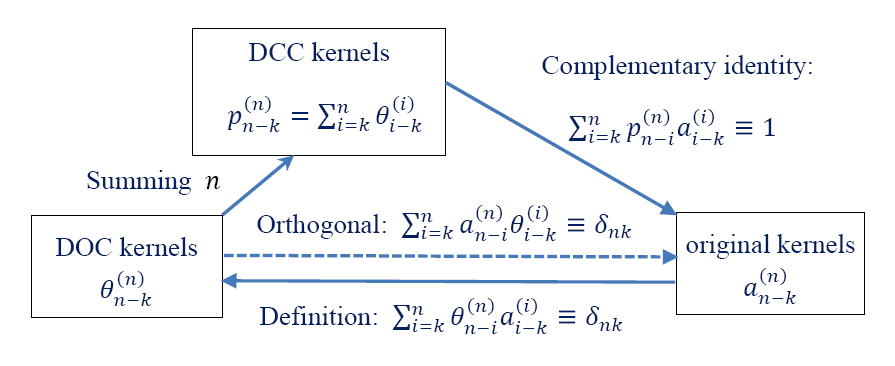
Figure 1: The relationship diagram of DOC and DCC kernels.

3 Proof of Theorem 1.1

With the preparations of Section 2, we are now ready to prove Theorem 1.1.

Proof of Theorem 1.1.

It follows from (2.19) and the definition (2.22) that

$$2\sum_{k=1}^{n}V_{k}\sum_{j=1}^{k}\theta_{k-j}^{(k)}V_{j}\geq\sum_{k=1}^{n}\Big{(}\sum_{j=1}^{k}\theta_{k-j}^{(k)}+p_{n-k}^{(n)}\Big{)}V_{k}^{2}\quad\text{for $n\geq 1$.}$$ (3.29)

Using (2.17) and (2.27) yields the following positivity result:

$$\sum_{j=1}^{k}\theta_{k-j}^{(k)}+p_{n-k}^{(n)}>0.$$

The above result, together with (3.29), confirms that the DOC kernels $\theta_{n-k}^{(n)}$ are positive definite. Then the desired result of Theorem 1.1 follows by using (2.8). ∎

Following the proof of Theorem 1.1, one can easily verify the following result.

Corollary 3.1.

For fixed $n\geq 2$, if the discrete convolution kernels $\big{\{}a^{(n)}_{n-k}\big{\}}_{k=1}^{n}$ satisfy

$$a^{(n)}_{j}\geq 0,\quad a^{(n-1)}_{j-1}\geq a^{(n)}_{j},\quad a^{(n-1)}_{j-1}a^{(n)}_{j+1}\geq a^{(n-1)}_{j}a^{(n)}_{j},\quad a^{(n)}_{j-1}\geq a^{(n)}_{j},$$

then the convolution kernels $a^{(n)}_{n-k}$ are positive semi-definite in the sense that

$$\sum_{k=1}^{n}w_{k}\sum_{j=1}^{k}a^{(k)}_{k-j}w_{j}\geq 0\qquad\text{for any sequence $\{w_{k}\}_{k=1}^{n}$.}$$

Proof.

We have $a^{(n)}_{0}>0$ unless the trial case with $a^{(n)}_{j}=0$ for $0\leq j\leq n-1$. If the discrete convolution kernels $a^{(n)}_{j}=0$ for $j\geq 1$, then the DOC kernels $\theta_{n-k}^{(n)}$ are positive semi-definite because $\psi^{(m)}_{\ell}=0$ for any $\ell\geq 1$ such that $\theta^{(n)}_{0}>0$ and $\theta^{(n)}_{j}=0$ for $j\geq 1$. Then using (2.8) confirms the claimed result. It remains to consider the case of $a^{(n)}_{0}\geq a^{(n)}_{1}>0$. In this case, similar to the proof of the proof for (2.17)-(2.18) gives

$$\theta_{0}^{(n)}>0,\quad\theta_{j}^{(n)}\leq 0\;\quad\text{for $1\leq j\leq n-1$,}$$

$$\sum_{j=1}^{n}\theta_{n-j}^{(n)}\geq 0.$$

Moreover, similar to the proof of (2.27) gives

$$p_{n-k}^{(n)}=\sum_{j=k}^{n}\theta_{j-k}^{(j)}\geq 0,\quad\text{for \;\; $1\leq k\leq n$.}$$

Hence, using (2.19) yields the positive semi-definiteness of the DOC kernels $\theta_{n-k}^{(n)}$, and then the desired result follows by using Lemma 2.1 by using (2.8). ∎

Corollary 3.1 presents another class of sufficient conditions for the positive semi-definiteness of discrete kernels $a^{(n)}_{n-k}$. Notice that if the discrete kernels are independent of the (time-level) index $n$, that is, $a^{(n)}_{j}=a_{j}$, then the conditions reduce to

$$a_{j}\geq 0,\quad a_{j-1}\geq a_{j},\quad a_{j-1}a_{j+1}\geq a_{j}^{2},$$

which are slightly stronger than (1.4) proposed in [13] since we have

$$2a_{j}\leq 2\sqrt{a_{j-1}a_{j+1}}\leq a_{j-1}+a_{j+1}.$$

4 Some applications of Theorem 1.1

In this section, we will apply Theorem 1.1 to study stability of some variable time-stepping schemes. Recall the definition of the Riemann–Liouville integral operator with order $\gamma>0$, (see, e.g., [21]):

$$(\mathcal{I}^{\gamma}v)(t):=\int_{0}^{t}\omega_{\gamma}(t-s)v(s)\,\mathrm{d}{s}\quad\text{for $t>0$,}\quad\text{where $\omega_{\gamma}(t):=\frac{t^{\gamma-1}}{\Gamma(\gamma)}.$}$$ (4.1)

On the other hand, the Caputo fractional derivative of order $\alpha$ is defined by

$$(\partial^{\alpha}_{t}v)(t):=(\mathcal{I}^{1-\alpha}v^{\prime})(t)=\int_{0}^{t}\omega_{1-\alpha}(t-s)v^{\prime}(s)\,\mathrm{d}{s}\quad\text{for $0<\alpha<1$.}$$ (4.2)

For a given $T>0$ and the time interval $[0,T]$, we consider a nonuniform time gird

$$0=t_{0}<t_{1}<\cdots<t_{k-1}<t_{k}<\cdots<t_{N}=T$$

with variable step-size $\tau_{k}:=t_{k}-t_{k-1}$ for $1\leq{k}\leq{N}$. The maximum time-step size is defined by $\tau:=\max_{1\leq{k}\leq{N}}\tau_{k}$. Also, we define the local time-step ratio as $r_{k}:=\tau_{k}/\tau_{k-1}$ for $k\geq 2$. For a mesh function $v^{k}=v(t_{k})$, we set $v^{k-\theta}:=(1-\theta)v^{k}+\theta v^{k-1}$, where $\theta\in[0,1)$ is a weighted parameter. Also, we define the following difference operators

$$\triangledown_{\!\tau}v^{k}:=v^{k}-v^{k-1}\quad\text{and}\quad\partial_{\tau}v^{k-\frac{1}{2}}:=\triangledown_{\!\tau}v^{k}/\tau_{k}.$$

4.1 L1 scheme for Caputo fractional derivative

Our first application is the variable-step L1 scheme for the Caputo fractional derivative (4.2). The L1 formula (see, e.g. [8]) uses $v^{\prime}(s)\approx\triangledown_{\!\tau}v^{k}/\tau_{k}$ in the subinterval $(t_{k-1},t_{k})$ to obtain

$$(\partial^{\alpha}_{\tau}v)^{n}:=\sum_{k=1}^{n}c^{(n,\alpha)}_{n-k}\triangledown_{\!\tau}v^{k}\quad\text{for $n\geq 1$,}$$

where the associated discrete L1 kernels read

$$c_{n-k}^{(n,\alpha)}:=\frac{1}{\tau_{k}}\int_{t_{k-1}}^{t_{k}}\omega_{1-\alpha}(t_{n}-s)\,\mathrm{d}{s}\quad\text{for $1\leq k\leq n$,}$$ (4.3)

By using the integral and differential mean value theorems, we have the following result.

Proposition 4.1.

The discrete L1 kernels $c_{n-k}^{(n,\alpha)}$ in (4.3) satisfy

$$c^{(n,\alpha)}_{j}>0,\quad c^{(n,\alpha)}_{j-1}>c^{(n,\alpha)}_{j},\quad c^{(n-1,\alpha)}_{j-1}>c^{(n,\alpha)}_{j},\quad c^{(n-1,\alpha)}_{j-1}c^{(n,\alpha)}_{j+1}>c^{(n-1,\alpha)}_{j}c^{(n,\alpha)}_{j}.$$

Then the discrete L1 kernels $c^{(n,\alpha)}_{n-k}$ are positive definite according to Theorem 1.1.

Proof.

For any fixed time-level index $n\geq 2$, the positivity and the decreasing property of $c^{(n,\alpha)}_{j}$ follow from the following fact which is due to the integral mean value theorem:

$$c^{(n,\alpha)}_{n-k}=\omega_{1-\alpha}(t_{n}-s_{nk})\quad\text{ for some $s_{nk}\in[t_{k-1},t_{k}]$}.$$

Consider an auxiliary sequence

$$\psi_{n-k}^{(n,\alpha)}:=\frac{c_{n-k}^{(n,\alpha)}}{c_{n-1-k}^{(n-1,\alpha)}}=\frac{c_{n,k}(1)}{c_{n-1,k}(1)}\quad\text{for $1\leq k\leq n-1$,}$$

where

$$c_{n,k}(\mu):=\frac{1}{\tau_{k}}\int_{t_{k-1}}^{t_{k-1}+\mu\tau_{k}}\omega_{1-\alpha}(t_{n}-s)\,\mathrm{d}{s}\quad\text{for $1\leq k\leq n$.}$$

Differentiating it with $\mu$ gives $c^{\prime}_{n,k}=\omega_{1-\alpha}(t_{n}-t_{k-1}-\mu\tau_{k})$. It follows from the Cauchy mean-value theorem that there exists some $\xi_{1k}\in(0,1)$ such that

$$\psi_{n-k}^{(n,\alpha)} = \frac{c_{n,k}(1)-c_{n,k}(0)}{c_{n-1,k}(1)-c_{n-1,k}(0)}=\frac{c_{n,k}^{\prime}(\xi_{1k})}{c_{n-1,k}^{\prime}(\xi_{1k})}$$ (4.4)

$$= \frac{\omega_{1-\alpha}(t_{n}-t_{k-1}-\xi_{1k}\tau_{k})}{\omega_{1-\alpha}(t_{n-1}-t_{k-1}-\xi_{1k}\tau_{k})}$$

$$= \Big{(}\frac{t_{n-1}-t_{k-1}-\xi_{1k}\tau_{k}}{t_{n}-t_{k-1}-\xi_{1k}\tau_{k}}\Big{)}^{\alpha}\qquad\text{for $1\leq k\leq n-1$}.$$

Note that the function $y=(A-x)/(B-x)$ is decreasing with respect to $x>0$ for $A<B$. Consequently,

$$\Big{(}\frac{t_{n-1}-t_{k}}{t_{n}-t_{k}}\Big{)}^{\alpha}<\psi_{n-k}^{(n,\alpha)}<\Big{(}\frac{t_{n-1}-t_{k-1}}{t_{n}-t_{k-1}}\Big{)}^{\alpha}\quad\text{for $1\leq k\leq n-1$,}$$

which yields

$$0<\psi_{1}^{(n,\alpha)}<\psi_{2}^{(n,\alpha)}<\cdots<\psi_{n-1}^{(n,\alpha)}<(t_{n-1}/t_{n})^{\alpha}<1\quad\text{for any fixed $n\geq 2$.}$$

This leads to the last two inequalities, and the proof is completed. ∎

Remark 4.1.

Recently, a second order L1⁺ formula was proposed in [6] for the Caputo derivatives:

$$(\partial_{\tau}^{\alpha}v)^{n-\frac{1}{2}}:=\frac{1}{\tau_{n}}\int_{t_{n-1}}^{t_{n}}\int_{0}^{t}\omega_{1-\alpha}(t-s)(\Pi_{1}v)^{\prime}(s)\,\mathrm{d}{s}\,\mathrm{d}{t}=\sum_{k=1}^{n}\bar{c}_{n-k}^{(n)}\triangledown_{\tau}v^{k}\quad\text{for $n\geq 1$,}$$

where the discrete L1⁺ kernels $\bar{c}_{n-k}^{(n)}$ are defined by

$$\bar{c}_{n-k}^{(n)}:=\frac{1}{\tau_{n}\tau_{k}}\int_{t_{n-1}}^{t_{n}}\int_{t_{k-1}}^{\min\{t,t_{k}\}}\omega_{1-\alpha}(t-s)\,\mathrm{d}{s}\,\mathrm{d}{t}\quad\text{for $1\leq{k}\leq{n}$.}$$ (4.5)

Note that the positive semi-definiteness of the continuous kernel $\omega_{1-\alpha}(t-s)$ directly leads to the positive semi-definite property of the discrete L1⁺ kernels $\bar{c}_{n-k}^{(n)}$ [6, Lemma 3.1]. However, it can be verified that the condition $\bar{c}_{0}^{(n)}\geq\bar{c}_{1}^{(n)}$ is may fail for some index $n$. In other words, Theorem 1.1 only provides some easy-to-check sufficient conditions. There is room for improvement, and it will be ideal to find sufficient and necessary conditions.

4.2 Energy stability for the time fractional Allen-Cahn equation

According to Proposition 4.1, on general nonuniform time meshes, Theorem 1.1 implies

$$\sum_{k=1}^{n}\triangledown_{\!\tau}v^{k}(\partial^{\alpha}_{\tau}v)^{k}=\sum_{k=1}^{n}\triangledown_{\!\tau}v^{k}\sum_{j=1}^{k}c^{(k,\alpha)}_{k-j}\triangledown_{\!\tau}v^{j}>0\quad\text{if $\triangledown_{\!\tau}v^{k}\not\equiv 0$.}$$ (4.6)

This result can be applied to study the energy stability of variable time stepping schemes for the time-fractional Allen-Cahn equation [25]:

$$\partial_{t}^{\alpha}u=\varepsilon^{2}\Delta{u}-F^{\prime}(u)\quad\text{for $x\in\Omega$ and $0<t\leq T$,}$$

where $\Omega$ is a bounded spatial domain, $\Delta$ is the Laplacian operator and $F(u)=\frac{1}{4}(1-u^{2})^{2}$ is the well known double well potential. It is known that for the time-fractional Allen-Cahn equation, there holds the following energy stability (see, e.g. [24, 25]):

$$E[u(t)]\leq E[u(0)]\quad\text{with}\quad E[u]:=\int_{\Omega}\Bigl{(}\varepsilon^{2}|\nabla u|^{2}+F(u)\Bigr{)}\,\mathrm{d}{x}.$$

It is thus desired to require that this stability holds at the discrete level. The following first-order explicit-implicit variable stabilization scheme was proposed in [5]:

$$\big{(}\partial_{\tau}^{\alpha}u\big{)}^{n} =\varepsilon^{2}D_{h}u^{n}-F^{\prime}(u^{n-1})-S(u^{n}-u^{n-1})\quad\text{for $n\geq{1}$,}$$ (4.7)

where $D_{h}$ denotes the discrete matrix of central difference approximation for Laplace operator $\Delta$ with periodic boundary conditions, and $S(u^{n}-u^{n-1})$ is a stabilization term with $S>0$ being a constant.

It is shown in [5, Theorem 2.2] that scheme (4.7) preserves the discrete maximum principle, but the the discrete energy stability proof is not provided. This is partially due to the complexity introduced by the non-uniform time steps. Using the positive definite property (4.6), one can now easily follow the proof of [5, Lemma 2.6] to obtain the following discrete energy stability result.

Proposition 4.2.

If the stabilized parameter $S\geq 2$, then the scheme (4.7) preserves the discrete maximum principle, together with the following discrete energy stability

$$E_{h}^{n}\leq E_{h}^{0}\quad\text{for $n\geq 1$},$$

where $E_{h}^{n}$ is the discrete energy, i.e.,

$$E_{h}^{n}=-\frac{\varepsilon^{2}}{2}(u^{n})^{T}D_{h}u^{n}+\sum_{{x}_{h}\in\Omega_{h}}F(u_{h}^{n}).$$

We remark that similar stability results on uniform time meshes has been presented in [5] and [25], while the above stability result on non-uniform grids seems to be new.

4.3 Numerical Riemann–Liouville integrals

As an example, we consider the following fractional wave equation [18, 21] that involves the fractional Riemann–Liouville integral:

$$\partial_{t}u=\mathcal{I}^{\gamma}\Delta u+f(x,t),\quad x\in\Omega,\quad 0<t\leq T.$$ (4.8)

It is known that the exact solution admits a weak singularity as $\partial_{tt}u\sim\mathcal{O}(t^{\gamma-1})$ near $t=0$. One of the effective ways to handle the initial singularity is to use nonuniform time grids, such as the graded meshes [18, 19, 8], to concentrate the time grids near $t=0.$

Similar to [7], let us consider the backward Euler time-stepping scheme for (4.8)

$$\partial_{\tau}u^{n-\frac{1}{2}}=\big{(}\mathcal{I}_{\tau}^{\gamma}\Delta u\big{)}^{n}+f(x,t_{n}),\quad n\geq 1,$$ (4.9)

where $\big{(}\mathcal{I}_{\tau}^{\gamma}v\big{)}^{n}$ represents the mid-point rule of fractional integral $\mathcal{I}^{\gamma}$

$$\big{(}\mathcal{I}_{\tau}^{\gamma}v\big{)}^{n}:=\sum_{k=1}^{n}c^{(n,1-\gamma)}_{n-k}\tau_{k}v^{k-\frac{1}{2}},\quad n\geq 1.$$ (4.10)

By Proposition 4.1, we see that

$$\sum_{k=1}^{n}\tau_{k}v^{k-\frac{1}{2}}(\mathcal{I}_{\tau}^{\gamma}v)^{k}=\sum_{k=1}^{n}\tau_{k}v^{k-\frac{1}{2}}\sum_{j=1}^{k}c^{(k,1-\gamma)}_{k-j}\tau_{j}v^{j-\frac{1}{2}}>0\quad\text{if $v^{k}\not\equiv 0$.}$$ (4.11)

By applying property (4.11) to (4.9), one easily gets the following stability estimate

$$\big{\|}u^{n}\big{\|}_{L^{2}}\leq\big{\|}u^{0}\big{\|}_{L^{2}}+\sum_{k=1}^{n}\tau_{k}\big{\|}f(t_{k})\big{\|}_{L^{2}}.$$

Note that such an $L^{2}$-norm estimate holds for a general class of nonuniform grids in time. By comparing with the previous stability analysis [18, 19, 20], which employed an discrete analogue to the positive semi-definiteness of the continuous kernel, the above analysis provides a more straightforward tool, i.e., by using only the properties of the discrete convolution kernels.

4.4 Numerical methods for weakly singular Volterra equations

We next present an application to Volterra integral equations of the form

$$\partial_{t}u=\mathcal{K}_{t}^{(\beta)}\Delta u+f(x,t),\quad x\in\Omega,\quad 0<t\leq T.$$ (4.12)

In (4.12), the convolution integral $\mathcal{K}_{t}^{(\beta)}v$ is defined by

$$\big{(}\mathcal{K}_{t}^{(\beta)}v\big{)}(t):=\int_{0}^{t}\kappa_{\beta}(t-s)v(s)\,\mathrm{d}{s},\quad t>0,$$ (4.13)

where $\kappa_{\beta}(t-s)>0$ is a general positive kernel. We assume that $\kappa_{\beta}^{\prime}<0$ and $\kappa_{\beta}^{\prime\prime}\geq 0$ which implies that the kernel $\kappa_{\beta}(t-s)$ is positive definite [17].

On a general non-uniform grid in time, applying the midpoint rule [3, 17, 20] for the convolution integral (4.13) gives

$$\big{(}\mathcal{K}_{\tau}^{(\beta)}v\big{)}^{k}:=\sum_{k=1}^{n}\kappa_{n-k}^{(n,\beta)}\tau_{k}v^{k-\frac{1}{2}},\quad n\geq 1,$$

where the discrete kernel is of the form

$$\kappa_{n-k}^{(n,\beta)}:=\frac{1}{\tau_{k}}\int_{t_{k-1}}^{t_{k}}\kappa_{\beta}(t_{n}-s)\,\mathrm{d}{s},\quad 1\leq k\leq n.$$ (4.14)

Note that $y=\kappa_{\beta}(t_{n}-x)/\kappa_{\beta}(t_{n-1}-x)$ is decreasing with respect to $t_{n-1}<x<t_{n}$ . Then one can follow similar argument as in Proposition 4.1 to verify the following result.

Proposition 4.3.

If $\kappa_{\beta}>0$, $\kappa_{\beta}^{\prime}<0$ and $\kappa_{\beta}^{\prime\prime}\geq 0$ , then the discrete convolution kernels $\kappa_{n-k}^{(n,\beta)}$ in (4.14) satisfy

$$\kappa_{j}^{(n,\beta)}>0,\quad\kappa_{j-1}^{(n,\beta)}>\kappa_{j}^{(n,\beta)},\quad\kappa_{j-1}^{(n-1,\beta)}>\kappa_{j}^{(n,\beta)},\quad\kappa_{j-1}^{(n-1,\beta)}\kappa_{j+1}^{(n,\beta)}\geq\kappa_{j}^{(n-1,\beta)}\kappa_{j}^{(n,\beta)}.$$

Consequently, the discrete kernels $\kappa_{n-k}^{(n,\beta)}$ are positive definite according to Theorem 1.1.

Now, consider the backward Euler time-stepping scheme for solving (4.12):

$$\partial_{\tau}u^{n-\frac{1}{2}}=\big{(}\mathcal{K}_{\tau}^{(\beta)}\Delta u\big{)}^{n}+f(x,t_{n}),\quad n\geq 1.$$ (4.15)

By Proposition 4.3, we see that

$$\sum_{k=1}^{n}\tau_{k}v^{k-\frac{1}{2}}(\mathcal{K}_{\tau}^{(\beta)}v)^{k}=\sum_{k=1}^{n}\tau_{k}v^{k-\frac{1}{2}}\sum_{j=1}^{k}\kappa^{(k,\beta)}_{k-j}\tau_{j}v^{j-\frac{1}{2}}>0\quad\text{if $v^{k}\not\equiv 0$.}$$ (4.16)

By applying (4.16) to the backward Euler scheme (4.15), it is easy to obtain the following $L^{2}$-norm estimate:

$$\big{\|}u^{n}\big{\|}_{L^{2}}\leq\big{\|}u^{0}\big{\|}_{L^{2}}+\sum_{k=1}^{n}\tau_{k}\big{\|}f(t_{k})\big{\|}_{L^{2}},\quad n\geq 1.$$

We emphasize again that this estimate is valid for a general class of non-uniform grid in time, including the well-studied graded meshes.

Remark 4.2.

For general convolution integrals (4.13) with smooth or weakly singular kernels, a second-order Crank-Nicolson formula was proposed by McLean et al. [17, 18]:

$$(\mathcal{K}_{\tau}^{(\beta)}v)^{n-\frac{1}{2}}:=\frac{1}{\tau_{n}}\int_{t_{n-1}}^{t_{n}}\int_{0}^{t}\kappa_{\beta}(t-s)v^{k-\frac{1}{2}}\,\mathrm{d}{s}\,\mathrm{d}{t}=\sum_{k=1}^{n}\bar{\kappa}_{n-k}^{(n)}\tau_{k}v^{k-\frac{1}{2}}\quad\text{for $n\geq 1$,}$$ (4.17)

where the associated discrete convolution kernels $\bar{\kappa}_{n-k}^{(n)}$ are defined by

$$\bar{\kappa}_{n-k}^{(n)}:=\frac{1}{\tau_{n}\tau_{k}}\int_{t_{n-1}}^{t_{n}}\int_{t_{k-1}}^{\min\{t,t_{k}\}}\kappa_{\beta}(t-s)\,\mathrm{d}{s}\,\mathrm{d}{t}\quad\text{for $1\leq{k}\leq{n}$.}$$ (4.18)

Again, the positive semi-definiteness of the continuous kernel directly implies the positive semi-definite property of the discrete kernels $\bar{\kappa}_{n-k}^{(n)}.$ Similar as in Remark 4.1, the condition C4 is not always fulfilled here because of the violation of $\bar{\kappa}_{0}^{(n)}\geq\bar{\kappa}_{1}^{(n)}$. Nevertheless, it is expected that our technique in proving Theorem 1.1 is still useful for handling this situation, and this will be investigated in a future work.

5 Concluding remarks

The positive definiteness of real quadratic forms with convolution structure plays an important role in analyzing variable time-stepping schemes for time-fractional differential equations and Volterra-type integral equations. In contrast to the classical treatments which use a discrete analogue to the positive semi-definiteness of continuous kernels, we present in this work a unified criteria obtained by using the DOC and DCC tools. More precisely, for convolution kernels $a^{(n)}_{n-k}$ we show for the first time some sufficient algebraic conditions that implies the positive definiteness of the associated real quadratic form. We emphasize the simplicity of the imposed conditions which are relevant to positivity (C1), monotonicity (C2 and C4), and convexity (C3). The usefulness and easy-to-check style are demonstrated in Section 4 where several first-order schemes are examined.

As noticed in Remarks 4.1-4.2, the condition C4 is not sharp for treating second-order discretization schemes. Nevertheless, similar situations occur even for the case of uniform grids. For example, the condition (1.4) of [13] works well for first-order schemes but failed for second-order approximations, see, e.g., [23]. On the other hand, it is expected that the condition C4 may be weakened so that our conditions are useful for high order time discretizations. A careful examination of the proof of Theorem 1.1 reveals that conditions C1-C3 together with the following inequality

$$p_{n-k}^{(n)}>-\sum_{j=1}^{k}\theta_{k-j}^{(k)}\quad\text{for $1\leq k\leq n$}$$ (5.1)

are sufficient for the positive definiteness claim. Note that the condition C4 ensures a stronger estimate $p_{n-k}^{(n)}\geq 0$, see (2.27). However, the weaker constraint (5.1) is quite complicated and not as elegant as desired. Some further efforts may be made in this direction.

References

• [1] H.-B. Chen, D. Xu, J. Cao and J. Zhou, A backward Euler alternating direction implicit difference scheme for the three-dimensional fractional evolution equation, Numer Methods Partial Differential Eq., 34 (2018), pp. 938–958.
• [2] E. Cuesta and C. Palencia, A fractional trapezoidal rule for integro-differential equations of fractional order in Banach spaces, App. Numer. Math., 45 (2003), pp. 139–159.
• [3] G. Fairweather, Spline collocation methods for a class of hyperbolic partial integro-differential equations, SIAM J. Numer. Anal., 31(2) (1993), pp. 444–460.
• [4] U. Grenander and G. Szegö, Toeplitz Forms and their Applications, Second (textually unaltered) edition, Chelsea Publishing Company, New York, 1984 (First edition publicated by University of California Press, Berkeley, CA, 1958).
• [5] B. Ji, H.-L. Liao and L. Zhang, Simple maximum-principle preserving time-stepping methods for time-fractional Allen-Cahn equation, Adv. Comput. Math., 46(2) (2020), doi: 10.1007/s10444-020-09782-2.
• [6] B. Ji, H.-L. Liao, Y. Gong and L. Zhang, Adaptive second-order Crank-Nicolson time-stepping schemes for time fractional molecular beam epitaxial growth models, SIAM J. Sci. Comput., 2020, 42(3) : B738-B760.
• [7] L. Li and D. Xu, Alternating direction implicit-Euler method for the two-dimensional fractional evolution equation, J. Comput. Phys., 236 (2013), pp. 157–168.
• [8] H.-L. Liao, D. Li and J. Zhang, Sharp error estimate of nonuniform L1 formula for linear reaction-subdiffusion equations, SIAM J. Numer. Anal., 56(2) (2018), pp. 1112-1133.
• [9] H.-L. Liao, W. McLean and J. Zhang, A discrete Grönwall inequality with application to numerical schemes for subdiffusion problems, SIAM J. Numer. Anal., 57(1) (2019), pp. 218-237.
• [10] H.-L. Liao, T. Tang and T. Zhou, A second-order and nonuniform time-stepping maximum-principle preserving scheme for time-fractional Allen-Cahn equations, J. Comput. Phys., (414) 2020, 109473.
• [11] H.-L. Liao and Z. Zhang, Analysis of adaptive BDF2 scheme for diffusion equations, Math. Comput., 2020, DOI: 10.1090/mcom/3585.
• [12] Y. Lin and C. Xu, Finite difference/spectral approximations for the time-fractional diffusion equation, J. Comput. Phys., 225(2) (2007), pp. 1533-1552.
• [13] J.C. López-Marcos, A difference scheme for a nonlinear partial integr-odifferential equation, SIAM J. Numer. Anal., 27 (1990), pp. 20–31.
• [14] C. Lubich, Convolution quadrature and discretized operational calculus I. Numer. Math. 52(1988), 129-145.
• [15] C. Lubich, Convolution quadrature and discretized operational calculus II. Numer. Math. 52(1988), 413-425.
• [16] C. Lubich, I.H. Sloan, and V. Thomée, Nonsmooth data error estimates for approximations of an evolution equation with a positive-type memory term, Math. Comp., 65 (1996), pp. 1–17.
• [17] W. McLean, V. Thomée, L. B. Wahlbin, Discretization with variable time steps of an evolution equation with a positive-type memory term, J. Comput. Appl. Math., 69 (1996), pp. 49-69.
• [18] W. McLean and K. Mustapha, A second-order accurate numerical method for a fractional wave equation, Numer. Math., 105 (2007), pp. 481–510.
• [19] K. Mustapha, An implicit finite difference time-stepping method for a subdiffusion equation with spatial discretization by finite elements, IMA J. Numer. Anal., 31 (2011), pp. 719-739.
• [20] A. K. Pani and G. Fairweather, An $H^{1}$-Galerkin mixed finite element method for an evolution equation with a positive-type memory term, SIAM J. Numer. Anal., 40(4) (2002), pp. 1475–1490.
• [21] I. Podlubny, Fractional differential equations, Academic Press, New York, 1999.
• [22] Z. Sun and X. Wu, A fully discrete difference scheme for a diffusion-wave system, App. Numer. Math., 56 (2006), pp. 193–209.
• [23] T. Tang, A finite difference scheme for partial integro-differential equations with a weakly singular kernel, App. Numer. Math., 11 (4) (1993), pp. 309–319.
• [24] T. Tang, Revisit of semi-implicit schemes for phase-field equations, To appear in Analysis in Theory and Applications, 2020.
• [25] T. Tang, H. Yu, and T. Zhou. On energy dissipation theory and numerical stability for time-fractional phase field equations, SIAM J. Sci. Comput., 41 (2019), pp. A3757–A3778.