Compressible potential flows around round bodies: Janzen-Rayleigh expansion inferences

Abstract

The subsonic, compressible, potential flow around a hypersphere can be derived using the Janzen-Rayleigh expansion (JRE) of the flow potential in even powers of the incident Mach number ${\mathcal{M}}_{\infty}$. JREs were carried out with terms polynomial in the inverse radius $r^{-1}$ to high orders in two dimensions (2D), but were limited to order ${\mathcal{M}}_{\infty}^{4}$ in three dimensions (3D). We derive general JRE formulae to arbitrary order, adiabatic index, and dimension. We find that powers of $\ln(r)$ can creep into the expansion, and are essential in 3D beyond order ${\mathcal{M}}_{\infty}^{4}$. Such terms are apparently absent in the 2D disk, as we confirm up to order ${\mathcal{M}}_{\infty}^{100}$, although they do show in other dimensions (e.g. at order ${\mathcal{M}}_{\infty}^{2}$ in 4D) and in non-circular 2D bodies. This suggests that the disk, which was extensively used to study basic flow properties, has additional symmetry. Our results are used to improve the hodograph-based approximation for the flow in front of a sphere. The symmetry-axis velocity profiles of axisymmetric flows around different prolate spheroids are approximately related to each other by a simple, Mach-independent scaling.

1 Introduction

While ideal flows (inviscid, with no heat conduction or additional energy dissipation effects; Landau & Lifshitz, 1959) are an extreme limit, they play an important role in research, for example (i) as a basis for more realistic flows, with additional effects such as viscosity; (ii) for modeling the bulk of weakly-interacting Bose-Einstein condensate (BEC) superfluids, which can be approximated as an inviscid, compressible fluid with a polytropic index $\gamma=2$; (iii) for modeling flow regimes which are not sensitive to the level of weak viscosity, such as in front of a round object; and (iv) for code validation and pedagogical reasons.

Janzen-Rayleigh expansions (JREs) can be broadly identified as an expansion of the flow variables in terms of the Mach number. JREs were used by Janzen (1913) and Rayleigh (1916) as a method to study D’Alembert paradox with the addition of compressibility effects. They considered an inviscid, compressible, subsonic flow of a fluid with a polytropic equation of state (EoS), with no external forces or initial vorticity. Specifically, a steady flow was assumed around a disk in two dimensions (2D) or around a sphere in three dimensions (3D), with an incident uniform flow far from the body. Introducing the flow potential, a scalar non-linear partial differential equation (PDE) was obtained, and expanded in the incident Mach number squared, ${\mathcal{M}}_{\infty}^{2}$.

Using the same setup, the JRE was used to solve the flow around various blunt objects (Goldstein & Lighthillm, 1944; Hasimoto, 1951; Hida, 1953; Longhorn, 1954; Imai, 1957; Kaplan, 1957; Van Dyke, 1958). The JRE has been generalized to several areas of research, such as vortex flows ( Moore & Pullin, 1991, 1998; Meiron, Moore & Pullin, 2000; Leppington, 2006; Crowdy & Krishnamurthy, 2018), porous channel flows (Majdalani, 2007; Maicke & Majdalani, 2008; Maicke, Saad & Majdalani, 2010; Cecil, Majdalani & Batterson, 2015), and acoustics (Slimon, Soteriou & Davis, 2000; Moon, 2013), and could be used in a wide range of other applications, as we demonstrate below.

The 2D flow around a disk has been researched extensively (Janzen, 1913; Rayleigh, 1916; Van Dyke & Guttmann, 1983; Guttmann & Thompson, 1993), for example in search for a solution to the transonic controversy, namely, “the existence, or non-existence, of a continuous transonic flow, that is, without a shock wave, around a symmetrical wing profile, with zero incidence with respect to the undisturbed velocity” (Ferrari, 1966). These and other problems that require a high-order expansion could not be explored as thoroughly in the 3D case, because previous JREs for the sphere were limited to second, i.e. ${\mathcal{M}}^{4}_{\infty}$, order (Kaplan, 1940; Tamada, 1940). Indeed, a power series in $r^{-1}$ yields a non-physical behaviour at the third, i.e. ${\mathcal{M}}^{6}_{\infty}$, expansion order. A higher order expansion in 3D is also needed, for example, to derive the flow in front of a sphere, in order to model axisymmetric bodies in various fields of physics ( Keshet & Naor, 2016, and references therein). Flows in higher dimensions, $d>3$, are also important, mainly for theoretical and pedagogical purposes.

We study the steady, inviscid, compressible flow around a hypersphere in $d$ spatial dimensions, and provide explicit results for the $d={2}$ (disk) and $d=3$ (sphere) cases. We derive the JRE in 3D beyond the presently available second-order, to an arbitrary order. As an example of the usage of such an expansion, we compare the axisymmetric flow in front of a sphere to that in front of a spheroid, and show that a simple scaling approximates the flow well for the prolate case. Furthermore, three orders in the JRE are sufficient to adequately describe these flows, for Mach numbers ranging from the incompressible to the sonic regimes.

The paper is organized as follows. In §2, we derive the JRE equations from the hydrodynamical ones. In §3, we show that each term in the JRE of the flow potential around a hypersphere is a finite sum of a product of powers of the radial coordinate, powers of its logarithm, and a set of orthogonal functions (Jacobi polynomials) of the polar coordinate. In §4, we outline the semi-analytic algorithm to compute the JRE and a numerical pseudospectral method we use to solve the non-linear compressible flow. We present results from our numerical solver and from the semi-analytical JRE, and highlight the compressibility to compute the JRE, in §5. The JRE is used to improve a hodographic approximation for the flow in front of the sphere in §6. In §7, we show that the axisymmetric flow in front of prolate spheroids is well approximated by that of the scaled flow in front of a sphere. We summarize and discuss our results in §8. In appendix §A, we provide explicit values of the coefficients of the series representation of the JRE for low orders of the flows around a disk and a sphere. Appendix §B discusses the hodographic approximation and general results. In appendix §C we detail the numerical solver.

2 Janzen-Rayleigh Expansion

Consider an isentropic flow in $d$-dimensions with no external forces of a perfect fluid with a polytopic, ideal gas EoS of adiabatic index $\gamma$,

$$p\propto{\rho^{\gamma}}\,.$$ (1)

The equations governing the flow are the continuity equation,

$$\frac{{\partial\rho}}{{\partial t}}+\bnabla\bm{\cdot}\left({\rho\bm{u}}\right)=0\,,$$ (2)

and the Euler equation,

$$\frac{{\partial{\bm{u}}}}{{\partial t}}+({\bm{u}}\bm{\cdot}\bnabla){\bm{u}}=-\frac{{\bnabla p}}{\rho}=-\frac{\bnabla c^{2}}{\gamma-1}\,.$$ (3)

Here, $\rho$, ${\bm{u}}$, and $p$ are respectively the mass density, velocity, and pressure, $c\equiv(dp/d\rho)^{1/2}=(\gamma p/\rho)^{1/2}$ is the sound velocity, and $\bnabla$ is the del operator in $d$-dimensions.

We henceforth assume a steady flow. Combining (1) and (2) to eliminate $\rho$ in favor of $c$ then yields

$$\frac{1}{\gamma-1}{\bm{u}}\bm{\cdot}\bnabla{c^{2}}=-{c^{2}}\bnabla\bm{\cdot}{\bm{u}}\,.$$ (4)

For our inviscid, steady flow, (3) yields the Bernoulli principle, namely, the quantity $w{\bm{u}}^{2}+c^{2}$ is constant along streamlines, where we define $w\equiv(\gamma-1)/2$.

We consider the flow along a body for a uniform flow incident from infinity,

$$c\left({r\to\infty}\right)={c_{\infty}}\quad\mbox{and}\quad{\bm{u}}\left({r\to\infty}\right)=u_{\infty}\bm{\hat{z}}\,,$$ (5)

where $r$ is the radial coordinate, $z$ is the coordinates along the flow, and the subscript $\infty$ indicates the far region, tending to spatial infinity. Using the boundary conditions (5) and the assumption that every streamline starts at infinity, the Bernoulli equation may be written as

$$w{{\bm{u}}^{2}}+c^{2}=w{{\bm{u}}_{\infty}^{2}}+c_{\infty}^{2}\,.$$ (6)

Considering the subsonic regime, we henceforth restrict the discussion to a potential flow, writing the velocity as the gradient of the flow potential,

$$\bm{u}\equiv\bnabla\phi\,.$$ (7)

Isolating $c^{2}$ from (6), substituting it into (4), and using the potential (7), we obtain a single PDE for the potential $\phi$ (Rayleigh, 1916),

$$\frac{1}{2}(\bnabla\phi)\bm{\cdot}\bnabla{\left({\bnabla\phi}\right)^{2}}=\left[w{u_{\infty}^{2}}+c_{\infty}^{2}-w{{{\left({\bnabla\phi}\right)}^{2}}}\right]{\nabla^{2}}\phi\,.$$ (8)

We normalize the variables to obtain them in a dimensionless form, by taking $\phi\to(u_{\infty}R)\phi$, and ${\bm{r}}\to R{\bm{r}}$ (which also normalize the velocity ${\bm{u}}\to u_{\infty}{\bm{u}}$), where $R$ is a characteristic length scale, for example the radius of a hypersphere. Defining ${\mathcal{M}}_{\infty}\equiv u_{\infty}/c_{\infty}$ as the Mach number at infinity, we then arrive at the dimensionless

$$\frac{1}{2}(\bnabla\phi)\bm{\cdot}\bnabla{\left({\bnabla\phi}\right)^{2}}=\left[{w+{{\mathcal{M}}_{\infty}^{-2}}-w{\left({\bnabla\phi}\right)}^{2}}\right]{\nabla^{2}}\phi\,.$$ (9)

We supplement this equation for the potential with two boundary conditions (BCs): the uniform incident flow from infinity, and the slip, no-penetration condition on the surface of the body (${\bm{\hat{n}}}\bm{\cdot}{\bm{u}}=0$), namely

$$\phi\left({r\to\infty}\right)=z=r\cos\theta\quad\mbox{and}\quad\bm{\hat{n}}\bm{\cdot}\bnabla\phi=0\,.$$ (10)

Here, $\bm{\hat{n}}$ is the normal to the body, and we use hyperspherical coordinates: a radial coordinate $0\leq r\leq\infty$, a polar angle $0\leq\theta\leq\pi$ measured with respect to the uniform flow at infinity, and $(d-2)$ additional angles. For axisymmetric flows such as in the case of a hypersphere, the flow is by symmetry independent of these additional angles.

To arrive at the JRE, we substitute the expansion

$$\phi{(\bm{r})}\equiv\sum\limits_{m=0}^{\infty}{{\phi_{m}(\bm{r})}{{\mathcal{M}}_{\infty}^{2m}}}$$ (11)

into (9), and isolate the different powers of ${\mathcal{M}}_{\infty}$. This leads to a recursive PDE for $\phi_{m}$ (for $m\geq 1$),

$${\nabla^{2}}{\phi_{m}} = -w{\nabla^{2}}{\phi_{m-1}}$$

$$+w\sum\limits_{\{{m_{1}},{m_{2}},{m_{3}}\}=0}^{m}{\delta_{{m_{1}}+{m_{2}}+{m_{3}},m-1}\left({\bnabla{\phi_{{m_{1}}}}\bm{\cdot}\bnabla{\phi_{{m_{2}}}}}\right){\nabla^{2}}{\phi_{{m_{3}}}}}$$

$$+\frac{1}{2}\sum\limits_{\{{m_{1}},{m_{2}},{m_{3}}\}=0}^{m}{\delta_{{m_{1}}+{m_{2}}+{m_{3}},m-1}\bnabla\left({\bnabla{\phi_{{m_{1}}}}\bm{\cdot}\bnabla{\phi_{{m_{2}}}}}\right)\bm{\cdot}\bnabla{\phi_{{m_{3}}}}}\,,$$

with an initial equation

$${\nabla^{2}}{\phi_{0}}=0\,,$$ (13)

along with BCs

$${\phi_{m}}\left({r\to\infty}\right)={\delta_{m,0}}r\cos\theta$$ (14)

at spatial infinity, and

$${\bm{\hat{n}}}\bm{\cdot}\bnabla{\phi_{m}}=0$$ (15)

on the body. Here, $\delta_{i,j}$ is the Kronecker delta symbol.

The zeroth-order equation (13) is the Laplace equation for $\phi_{0}$, corresponding to the incompressible limit ${\mathcal{M}}_{\infty}\to 0$. For higher orders, equation (2) can be regarded as a set of Poisson equations for $\phi_{m}$ at each order $m$, with a source term being a function of the lower-order solutions, $\{\phi_{i}\}^{m-1}_{i=0}$, and their derivatives. In general, the solution to (2) at any order $m\geq 1$ under the BCs (14) and (15) is a sum of an inhomogeneous solution and a homogeneous solution,

$$\phi_{m}=\phi_{m}^{\rm{(in)}}+\phi_{m}^{\rm{(ho)}},$$ (16)

where $\phi_{m}^{\rm{(ho)}}$ solves the Laplace equation.

The JRE (11) is constructed by iteratively determining the functions $\phi_{m}$. One starts by deriving $\phi_{0}$, obtained as the solution to the zeroth-order Laplace equation (13) under the BCs. Increasingly higher-order functions $\phi_{m}$ are then incrementally derived, by solving the corresponding Poisson equations (2) under the same BCs. At each order $m\geq 1$, the inhomogeneous solution $\phi_{m}^{\rm{(in)}}$ is fixed by the source term in the corresponding (2), which is explicitly written once all lower order functions $\phi_{m}$ are determined. This solution is then combined with an expansion $\phi_{m}^{\rm{(ho)}}$ of homogenous solutions, the coefficients of which are determined by applying the BCs to the resulting (16).

3 JRE for a hypersphere

Simple solutions exist for the flow around a $d$-dimensional hypersphere, for which the Laplace equation has known analytic solutions, and the Poisson equation is easily solved. Choosing the characteristic length $R$ as the hypersphere radius, the normalized slip BC (15) here simplifies to

$$\partial_{r}\phi\left(r=1,\theta\right)=0\,.$$ (17)

Considering the hyperspherical and axial symmetries, it is useful to write the general solution to the Laplace equation (13) as the infinite sum of positive and negative radial powers (Feng et al., 2011)

$$\sum\limits_{n=1}^{\infty}{\left(A_{n}r^{n}+B_{n}r^{-n-d+2}\right){\mathcal{J}}_{n}^{(d)}\left(\mu\right)},$$ (18)

where we define $\mu\equiv\cos\theta$, the normalized Jacobi polynomials

$${\mathcal{J}}_{n}^{(d)}\left({\mu}\right)\equiv\frac{{J_{n}^{\left({\frac{{d-3}}{2},\frac{{d-3}}{2}}\right)}\left({\mu}\right)}}{{J_{n}^{\left({\frac{{d-3}}{2},\frac{{d-3}}{2}}\right)}\left(1\right)}}=\frac{C_{n}^{\left(\frac{d}{2}-1\right)}(\mu)}{{{n+d-3}\choose{n}}}\,,$$ (19)

and numerical coefficients $A_{n}$ and $B_{n}$. Here, $J_{n}^{(\alpha,\beta)}(\mu)$ and $C_{n}^{(\alpha)}(\mu)$ are respectively the standard Jacobi and Gegenbauer polynomials.

The source term in (2) is a sum of multiple terms, each composed of even derivatives in $\theta$ and odd multiples of functions $\phi$. Therefore, the polar dependence will always exhibit the same symmetry as the zero-order solution $\phi_{0}$. As the hypersphere is isotropic, the incompressible flow also shows a backward-forward symmetry. We conclude that the functions ${\mathcal{J}}_{n}^{(d)}$ appearing in $\phi_{m}$ on all orders $m$ have only odd $n$. Next, we construct the hypersphere JRE by considering increasingly larger orders $m$.

3.1 Zeroth order: $m=0$

For the $m=0$ order, the infinity BC (14) allows only the radially linear and decaying terms in the solution (18). The slip BC (17) restricts the solution further, allowing for only the decaying term proportional to ${\mathcal{J}}_{1}^{(d)}(\mu)=\mu$. The solution to the Laplace equation (13) around a $d$-dimensional hypersphere thus becomes

$$\phi_{0}^{(d)}(r,\theta)=\left[{r+\frac{1}{{\left({d-1}\right){r^{d-1}}}}}\right]\cos\theta\,.$$ (20)

Henceforth, we omit the dimension superscript $(d)$ unless necessary.

3.2 First order: $m=1$

The first-order potential, $\phi_{1}$, is determined by

$${\nabla^{2}}{\phi_{1}} = -w{\nabla^{2}}{\phi_{0}}+\frac{1}{2}\left(\bnabla{\phi_{{0}}}\right)\bm{\cdot}\bnabla\left(\bnabla{\phi_{{0}}}\right)^{2}+w\left(\bnabla{\phi_{{0}}}\right)^{2}{\nabla^{2}}{\phi_{0}}\,,$$ (21)

which, by the zeroth-order (13), simplifies to

$${\nabla^{2}}{\phi_{1}} = \frac{1}{2}\left(\bnabla{\phi_{{0}}}\right)\bm{\cdot}\bnabla\left(\bnabla{\phi_{{0}}}\right)^{2}.$$ (22)

Plugging the $m=0$ solution (20) into (22) gives the Laplace equation with the explicit source term,

$${\nabla^{2}}{\phi_{1}} = \left[-3\mu+\left(2+d\right)\mu^{3}\right]r^{-d-1}\frac{d}{d-1}+\left[\left(-3+d\right)\mu+\left(2+d-d^{2}\right)\mu^{3}\right]r^{-2d-1}\frac{2d}{\left(d-1\right)^{2}}$$ (23)

$$+\left[\left(-3+2d\right)\mu+\left(2+d-3d^{2}+d^{3}\right)\mu^{3}\right]r^{-3d-1}\frac{d}{\left(d-1\right)^{3}}\,.$$

The orthogonal decomposition of Jacobi polynomials (Chaggara & Koepf, 2010) then yields

$${\nabla^{2}}{\phi_{1}} = {\mathcal{J}}_{3}\left({\mu}\right)r^{-d-1}d$$

$$+ \left[-2d{\mathcal{J}}_{1}\left({\mu}\right)-\left(1+d\right)\left(d-2\right){\mathcal{J}}_{3}\left({\mu}\right)\right]r^{-2d-1}\frac{2d}{\left(d-1\right)\left(d+2\right)}$$

$$+ \left[d\left(-4+3d\right){\mathcal{J}}_{1}\left({\mu}\right)-\left(1+d-d^{2}\right)\left(d-2\right){\mathcal{J}}_{3}\left({\mu}\right)\right]r^{-3d-1}\frac{d}{\left(d-1\right)^{2}\left(d+2\right)}\,.$$

This result may be compactly written in the form

$${\nabla^{2}}\phi_{1}=\sum\limits_{k,n}{s^{(\rm{in})}_{1,k,n}{r^{k}}{\mathcal{J}}_{n}\left({\mu}\right)}\,,$$ (25)

where $s^{(\rm{in})}_{m,k,n}$ are the expansion coefficients of the order-$m$ Poisson source term, for radial order $k$ and angular order $n$.

As the Poisson equation is linear, suffice to solve, for arbitrary $k$ and $n$, the equation

$${\nabla^{2}}\phi_{k,n}={r^{k}}{\mathcal{J}}_{n}\left({\mu}\right)\,.$$ (26)

This equation has the particular, inhomogeneous solution

$$\phi_{k,n}^{(\rm{in})}=\frac{{{r^{k+2}}{\mathcal{J}}_{n}\left({\mu}\right)}}{{(k+2)\left({k+d}\right)-n\left({n+d-2}\right)}}\,,$$ (27)

provided that $k\notin\{-d-n,n-2\}$. These two exceptional values of $k$ do not occur at order $m=1$, as seen from (3.2), but they may appear at higher orders, as discussed below in §3.3. We may now expand the inhomogeneous solution as

$$\phi^{\rm{(in)}}_{1}=\sum\limits_{k,n}{s^{(\rm{in})}_{1,k,n}\phi^{\rm{(in)}}_{k,n}}\,,$$ (28)

where the numerical coefficients $s^{(\rm{in})}_{1,k,n}$ are determined by equating (3.2) and (25).

From (3.2) and (27) we see that the largest (i.e. least negative) power of $r$ for $m=1$ is $k_{max}=-d+1<0$, implying that $\phi^{\rm{(in)}}_{1}$ includes only radially declining terms. For higher orders, (2) combines the derivatives of multiple $\phi_{m}$ functions, but the highest radial power $k_{max}$ in the source term remains no larger than $-d-1$. Consequently, the inhomogeneous solution for all $m\geq 1$ orders includes only radially declining terms. This conclusion, combined with the BCs, indicate that the homogeneous solution may be expanded with only negative powers of $r$ for any $m>0$,

$$\phi^{\rm{(ho)}}_{m>0}=\sum\limits_{n=1}^{\infty}{s^{(\rm{ho})}_{m,n}{r^{-n-d+2}}{\mathcal{J}}_{n}\left(\mu\right)}\,,$$ (29)

where $s^{(\rm{ho})}_{m,n}$ are numerical coefficients, to be determined below.

The full solution for $m=1$ now becomes

$$\phi_{1}=\phi_{1}^{\rm{(in)}}+\phi_{1}^{\rm{(ho)}}=\sum\limits_{k,n}{s_{1,k,n}r^{k}{\mathcal{J}}_{n}\left(\mu\right)},$$ (30)

where we introduced the numerical coefficients

$$s_{1,k,n}=\frac{s^{(\rm{in})}_{1,k-2,n}}{k(k+d-2)-n(n+d-2)}+s^{(\rm{ho})}_{1,n}\delta_{k,-n-d+2}\,.$$ (31)

These coefficients may now be determined from the slip BC (17),

$$\frac{\partial\phi_{1}}{\partial r}(r=1)=\sum\limits_{k,n}{ks_{1,k,n}{\mathcal{J}}_{n}\left(\mu\right)}=0\,,$$ (32)

implying that

$$s^{(\rm{ho})}_{1,n}=\frac{1}{n+d-2}\sum\limits_{k,n}{\frac{ks^{(\rm{in})}_{1,k-2,n}}{k(k+d-2)-n(n+d-2)}}\,.$$ (33)

As the coefficients $s^{(\rm{in})}_{1,k,n}$ are known from (3.2) and (25), the solution (30) is completely specified by (31) and (33).

3.3 Higher orders: $m\geq 2$

Substituting $\phi_{0}$ and $\phi_{1}$ in the Poisson equation (2) for the next, $m=2$ order, results again in an equation of the form (25), but now for $\phi_{2}$ and with different coefficients. Equations of the same form persist for increasingly higher orders $m$, as long as the source term in (2) is free of non-zero terms $s_{m,k,n}$ which satisfy one of the aforementioned special conditions, $k=-d-n$ or $k=n-2$. Indeed, the source term consists of differential operators of the form $\nabla^{2}f(r,\mu)$ and $\bnabla f(r,\mu)\cdot\bnabla g(r,\mu)$, where $f$ and $g$ are constructed from lower order $\phi$ terms. As long as $f$ and $g$ are sums of terms, each of which is a product of powers of $r$ and Jacobi polynomials in $\mu$, the source term would remain of the form (25).

For the special cases $k\in\{-d-n,n-2\}$, the solution to (26) is no longer given by (27), which formally diverges. It is sufficient to consider the former case, $k=-d-n$, as the latter, $k=n-2$, is then obtained by the transformation $n\to-n-d+2$, under which ${\mathcal{J}}_{n}^{(d)}$ remains invariant. Here, the inhomogeneous solution to (26) becomes

$$\phi_{k=-d-n,n}=-\frac{{\Gamma\left[{2,\left({2n+d-2}\right)\ln\left(r\right)}\right]}}{{{{\left({2n+d-2}\right)}^{2}}}}{r^{n}}{\mathcal{J}}_{n}\left({\mu}\right)\,,$$ (34)

where $\Gamma(x,y)$ is the incomplete Gamma function, defined by

$$\Gamma\left({x,y}\right)=\int\limits_{y}^{\infty}{{t^{x-1}}{e^{-t}}dt}\,.$$ (35)

Once a $\ln(r)$ term of (34) appears in the inhomogeneous solution for $\phi_{m}$, as a result of a special $k$ term in the source-term expansion (25), a power-series in $r$ as in (30) is no longer sufficient. Indeed, when $x=\ell+1$ and $y=p\ln\left(r\right)$ for integers $\ell$ and $p$,

$$\Gamma\left[{\ell+1,p\ln\left(r\right)}\right]=\frac{{\ell!}}{{{r^{p}}}}\sum\limits_{j=0}^{\ell}{\frac{{{{\left[p\ln\left(r\right)\right]}^{j}}}}{{j!}}}$$ (36)

contains logarithmic, and not only polynomial, radial terms. Since $\ln(r)$ cannot be expanded as a power series of $r^{-1}$ valid over the full $1\leq r<\infty$ range, one must then take into account logarithmic terms in the expansion of $\phi_{m}$ and in the resulting source terms of higher order functions.

Generalizing the prototypical source term in (25) to include a logarithm of $r$ to some power $l$, we must therefore also consider the generalized equation

$${\nabla^{2}}\phi_{k,n,\ell}=r^{k}{\mathcal{J}}_{n}\left({\mu}\right)\ln^{\ell}\left(r\right)\,.$$ (37)

As long as $k$, $d$, and $n$ do not satisfy one of the special cases

$$k\in\{-d-n,n-2\}\,,$$ (38)

the inhomogeneous solution to this equation is

$$\phi_{k,n,\ell} = \frac{{{\mathcal{J}}_{n}\left({\mu}\right)}}{{2n+d-2}}\left({r^{-n-d+2}}\frac{{\Gamma\left[{\ell+1,\left({-d-k-n}\right)\ln\left(r\right)}\right]}}{{{{\left({-d-k-n}\right)}^{\ell+1}}}}\right.$$ (39)

$$\left.-{r^{n}}\frac{{\Gamma\left[{\ell+1,\left({n-k-2}\right)\ln\left(r\right)}\right]}}{{{{\left({n-k-2}\right)}^{\ell+1}}}}\right)\,,$$

whereas for $k=-d-n$ we find

$$\phi_{k=-d-n,n,\ell}=-{r^{n}}{\mathcal{J}}_{n}\left({\mu}\right)\frac{{\Gamma\left[{\ell+2,\left({2n+d-2}\right)\ln\left(r\right)}\right]}}{{{{\left(\ell+1\right)\left({2n+d-2}\right)}^{\ell+2}}}}\,.$$ (40)

The case $k=n-2$ is again obtained using the transformation $n\to-n-d+2$.

$$\phi_{k=-n-d+2,n,\ell}=-{r^{-n-d+2}}{\mathcal{J}}_{n}\left({\mu}\right)\frac{{\Gamma\left[{\ell+2,\left({-2n-d+2}\right)\ln\left(r\right)}\right]}}{{{{\left(\ell+1\right)\left({-2n-d+2}\right)}^{\ell+2}}}}\,.$$ (41)

The overall solution for $\phi_{m}$ may now be expanded as the finite sum

$$\phi_{m}=\sum\limits_{k,n,\ell}{s_{m,k,n,\ell}r^{k}{\mathcal{J}}_{n}^{(d)}\left({\mu}\right)\ln^{\ell}\left(r\right)}\,,$$ (42)

where the numerical coefficients $s_{m,k,n,\ell}$ are determined using the BCs in analogy with the above $m=2$ discussion. The expansion (42) is complete, as the inhomogeneous solution yields only powers of $r$ and $\ln\left(r\right)$, and the homogeneous solution yields only powers of $r$, so the resulting higher-order source terms are again of the form (37).

One can prove, by induction, the following rules for the $m\geq 1$ indices in (42),

$$1-d-2md\leq k\leq 1-d$$ (43)

and

$$1\leq n\leq 1+2m\,;$$ (44)

the summation limits for the logarithmic term are discussed in §5.

4 Semi-analytical and numerical solvers for disk and sphere flows

We explicitly solve equation (2) for the hypersphere in the $d=2$ and $d=3$ cases, namely, we derive the flows around a 2D disk and around a 3D sphere. The normalized Jacobi functions reduce to the Chebyshev polynomials ${T_{n}}$ in 2D,

$${\mathcal{J}}_{n}^{(2)}\left({\cos\theta}\right)={T_{n}}\left({\cos\theta}\right)=\cos\left({n\theta}\right)\,,$$ (45)

and to the Legendre polynomials ${P_{n}}$ in 3D,

$${\mathcal{J}}_{n}^{(3)}\left({\cos\theta}\right)={P_{n}}\left({\cos\theta}\right)\,.$$ (46)

As discussed in §3, we consider the generalized expansion (11) and (42) of the flow potential in each case,

$$\phi^{\rm{disk}}=\left(r+\frac{1}{r}\right)\cos\theta+\sum\limits_{m=1}^{\infty}{\sum\limits_{\ell=0}^{\infty}{\sum\limits_{n=1}^{2m+1}{\sum\limits_{k=-1-4m}^{-1}{a_{m,k,n,v}{{\mathcal{M}}_{\infty}^{2m}}{r^{k}}\cos\left({n\theta}\right){{\ln}^{\ell}}\left(r\right)}}}}$$ (47)

and

$$\phi^{\rm{sphere}}=\left(r+\frac{1}{2r^{2}}\right)\mu+\sum\limits_{m=1}^{\infty}{\sum\limits_{\ell=0}^{\infty}{\sum\limits_{n=1}^{2m+1}{\sum\limits_{k=-2-6m}^{-2}{{b_{m,k,n,\ell}}{{\mathcal{M}}_{\infty}^{2m}}{r^{k}}{P_{n}}\left(\mu\right){{\ln}^{\ell}}\left(r\right)}}}}\,,$$ (48)

where $a$ and $b$ are the expansion coefficients in 2D and 3D, respectively and the summation index $n$ takes only odd values.

We compute these JREs analytically, following the steps outlined in §3. The $m=0$ term is obtained from (20). For each order $m>0$, we compute the source terms on the RHS of (2), and decompose them into a sum of terms proportional to $r^{k}{\mathcal{J}}_{n}({\mu})\ln^{\ell}(r)$ as in (37). The inhomogeneous solution $\phi^{\rm{(in)}}_{m}$ is then obtained as the corresponding sum of solutions of the form (39)–(41), and added to the homogeneous solution $\phi^{\rm{(ho)}}_{m}$ of (29). The coefficients ${s^{(\rm{ho})}_{m,n}}$ in the latter sum are determined from the slip BC, as demonstrated for $m=1$ in (33). This process is repeated until the necessary accuracy of the JRE is reached.

The JRE results are compared to the flow obtained from a numerical solution to the non-linear equation (9). We follow Pham et al. (2005) and use the pseudospectral collocation method (Boyd, 2001) for a fast convergence. In the pseudospectral method, the solution to a PDE is expanded in terms of base functions, each being a product of individual (and typically orthogonal) functions for each coordinate. In collocation methods, the PDE is then evaluated and solved at a set of points, usually taken as the roots of the basis functions. This leads to a set of linear equations for the basis function coefficients, which are solved to give an approximate PDE solution. In general for pseudospectral methods, if the solution is smooth (all derivatives of all orders are continuous) then the convergence is exponential in the number $N$ of collocation points (Boyd, 2001), $O\left(e^{-N}\right)$.

Pham et al. (2005) use the Chebyshev-Fourier set of basis functions, invoking $\cos(n\theta)$ and $\sin(n\theta)$ with integer $n$ as angular basis functions. As discussed in §3, the analytical solution for $\phi$ is a sum of $\cos(n\theta)$ with odd positive $n$, so we expand the flow potential in odd cosine functions. To achieve the same accuracy as Pham et al. (2005), we need only a fourth of the angular basis functions.

For the radial part, we apply an inversion map $\varrho\equiv r^{-1}$ and expand in Chebyshev Polynomials $T_{k}(\varrho)$, to resolve both small and large $r$ behavior. The pseudospectral expansion thus becomes

$${\phi_{\rm{ps}}}=\phi_{0}+\sum\limits_{k=0}^{k_{\max}}\sum\limits_{n=0}^{n_{\max}}{{c_{k,n}}{T_{k}}\left(\varrho\right)\cos\left[{\left({2n+1}\right)\theta}\right]}\,.$$ (49)

Here, $k_{max}$ and $n_{max}$ are the radial and angular resolution, i.e. the number of collocation points, and $c_{k,n}$ are real coefficients. The BCs are guarantees if they are satisfied by the potential $\phi_{0}$, chosen as the incompressible solution (20). Since the effective computational domain and symmetry are the same in our 2D and 3D frameworks, we expand both flows, around a disk and around a sphere, in the same basis functions (49). Appendix §C provides more details on the the calculations of $c_{k,n}$ and demonstrates the numerical convergence.

5 Results

We calculate the JRE (47) and (48) up to order $m=30$ for the disk and $m=18$ for the sphere. Appendix §A provides explicit expressions for the coefficients $a$ and $b$ up to order $m=3$ (i.e. ${\mathcal{M}}_{\infty}^{6}$) for a general $\gamma$. For the pseudospectral code we use a resolution up to 32 Chebyshev and 64 odd cosine functions, but as shown below, much lower orders and resolutions are sufficient to capture the behaviour of the flow (see figure 2 and 6). The results are presented in the following figures mainly for $\gamma=7/5$. Different choices of $\gamma$ give qualitatively similar results, as demonstrated for $\gamma=5/3$ in figure 3b.

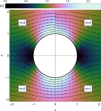
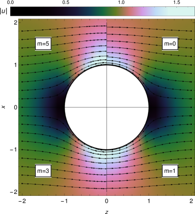
Figure 1: JRE solution to the critical flow around a unit-hypersphere (white disk) for $\gamma=7/5$ in 2D (a unit disk; left panel; incident near-critical Mach number ${\mathcal{M}}_{\infty}={\mathcal{M}}^{\rm{disk}}_{c}\simeq 0.3982$) and 3D (a unit sphere; right panel; ${\mathcal{M}}^{\rm{sphere}}_{c}\simeq 0.5619$). In such a critical flow, the Mach number at the equator of the body locally reaches ${\mathcal{M}}_{\rm{eq}}=1$. Streamlines (arrows) represent the trajectory of the flow (passing through equidistant points at $z=\pm 2$ (black dots). The normalized (dimensionless) speed $|u|$ is computed up to different JRE orders $m$ (of ${\mathcal{M}}_{\infty}^{2}$ in (11); see labels) in each quadrant. The effect of compressibility is particularly noticeable by comparing the $m=0$ and $m=5$ approximations along the $x>0$ axis.

Figure 1 shows the flow around a disk (left panel) and a sphere (right panel) for incident Mach numbers at infinity approaching the respective critical/sonic Mach numbers. The latter are tuned to yield a sonic flow at the equator of the hypersphere, ${\mathcal{M}}(r=1,\theta=\pi/2)=1$, leading to ${\mathcal{M}}^{\rm{disk}}_{c}\simeq 0.3982$ in 2D and ${\mathcal{M}}^{\rm{sphere}}_{c}\simeq 0.5619$ in 3D. The color intensity (cubehelix; Green, 2011) in the figure represents the normalized speed $|u|$. The flow is symmetric under both $x$ and $z$ reflections, i.e. $\theta\to-\theta$ and $\theta\to\pi-\theta$, so it is sufficient to plot only one quadrant of the $x-z$ plane. We thus utilize all four quadrants to show the differences between the JRE obtained up to different, $m=0$ to $m=5$, orders (see labels). To show the JRE corrections to the flow, we plot the streamlines (arrows) that pass through a set of equidistant points at $x=\pm 2$, so the differences between quadrant arrows are meaningful. Comparing the different quadrants shows that the compressible effects captured by higher orders $m$ raise the velocity and lower the density in the equatorial plane; most but not all of the change already transpires as $m=0$ is raised to $m=1$.

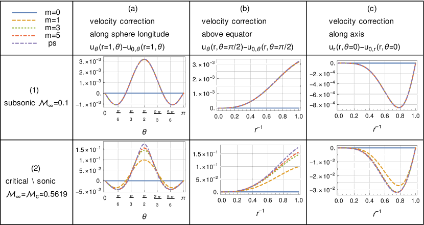
Figure 2: Compressible corrections to the flow around a 3D sphere for $\gamma=7/5$ according to different JRE orders and to the pseudospectral (ps) solver (see legend). Profiles are shown for the flow along the longitude of the sphere (column a), at different radii above the equator (column b), and along the symmetry axis (column c), for both a subsonic flow with ${\mathcal{M}}_{\infty}=0.1$ (row 1) and for the critical flow (row 2).

Figure 2 shows the compressible contribution to the flow around a sphere; qualitatively similar results are obtained for the disk. The contribution is computed based on JREs of different orders, as well as on the numerical solution, and shown for the polar velocity on the sphere (column a), the polar velocity at the equatorial plane (column b), and the radial velocity along the symmetry axis (column c). We plot these profiles for two different flows, with incident Mach numbers ${\mathcal{M}}_{\infty}=0.1$ to demonstrate a subsonic case (row 1), and ${\mathcal{M}}_{\infty}={\mathcal{M}}_{c}\simeq 0.5619$ for the critical case (row 2). As seen from row 1, at low Mach numbers, the JRE converges rapidly; the $m=1$ JRE is sufficient for accurately (within $\sim 0.005\%$ in $\bm{u}$ for ${\mathcal{M}}_{\infty}=0.1$) capturing the compressible effects. Convergence is slower for larger ${\mathcal{M}}_{\infty}$, but manageable (compressible effects captured within $\sim 5\%$ in $\bm{u}$ for $m=1$) even in the critical limit.

For the flow around a disk in 2D, we find no logarithmic terms in the flow potential, for any $\gamma$. Namely, all computed JRE (47) coefficients $a$ with $\ell\neq 0$ vanish, as illustrated in table 2 up to $m=3$ order. We confirm this behavior for arbitrary $\gamma$ up to order $m=30$. Using a prescribed $\gamma$ speeds up the JRE computations, allowing us to reach higher orders. We thus compute the JRE up to order $m=50$ for the specific cases $\gamma\in\{1,7/5,5/3,2\}$, corresponding respectively to isothermal, ideal diatomic, ideal monatomic, and weakly-interacting bose, gasses. In all of these cases, we find no logarithmic terms in the flow potential.

In contrast, logarithmic terms are unavoidable in the flow around a sphere in 3D, for any $\gamma$. Indeed, the JRE (48) shows the first logarithmic term at order $m=3$, for $k=-8$, $n=7$ and $\ell=1$, as indicated in table 4. This coefficient is proportional to $5+7\gamma+2\gamma^{2}$, which vanishes only for negative, non-physical $\gamma$ values. In addition to such $\ell=1$ terms for order $m\geq 3$, we find $\ell=2$ terms for order $m\geq 6$, $\ell=3$ terms for order $m\geq 9$, and so on, with the highest logarithmic term order increasing by one every three orders in $m$. Furthermore, the term with the highest logarithm power is also proportional to $\propto{r^{-2m-2}P_{2m+1}(\mu)}$. This behavior is verified up to order $m=18$ for arbitrary $\gamma>-1$, and up to order $m=30$ for the specific values of $\gamma$ chosen above.

While proving that these effects persist as $m$ increases to infinity is beyond the scope of the present work, we hypothesize that they do:

Conjecture 1

Logarithmic JRE terms never appear in the flow of a polytropic $\gamma\geq 1$ fluid around a disk.

Conjecture 2

For the flow around a sphere, the highest $\ell$ of JRE terms $\propto{{\mathcal{M}}_{\infty}^{2m}}{{\ln}^{\ell}(r)}$ is $\ell_{max}=\lfloor m/3\rfloor$.

6 Example: axial hodographic approximation

(a)

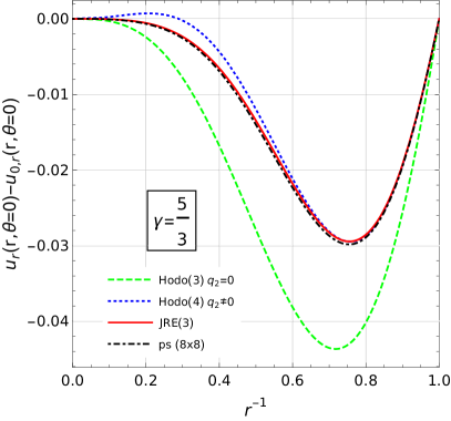
(b)

Figure 3: Compressibility contribution to the velocity along the symmetry axis of a sphere near the critical Mach number, for $\gamma=7/5$ (left panel, ${\mathcal{M}}_{\infty}={\mathcal{M}}_{c}\simeq 0.5619$) and $\gamma=5/3$ (right panel, ${\mathcal{M}}_{\infty}={\mathcal{M}}_{c}\simeq 0.5462$). Results shown for a converged pseudospectral calculation (ps, dotted-dashes black curve), a third order JRE (JRE(3), solid red) and hodographic approximations with (Hodo(4), dotted blue) and without (Hodo(3), dashed green) the $q_{2}$ coefficient.

	$m=0$	$m=1$	$m=2$	$m=3$	$m=4$
$q_{0}$	$1.5$	$1.3809$	$1.3783$	$1.3766$	$1.3762$
$q_{1}$	$-0.5$	$-0.5$	$-0.5$	$-0.5$	$-0.5$
$q_{2}$	$0$	$0.0254$	$0.0259$	$0.0263$	$0.0265$
$q_{3}$	$0$	$0.0585$	$0.0662$	$0.0689$	$0.0688$

Table 1: Coefficients of the first four terms in the Taylor expansion of $q\left(u\right)$, for different JRE orders $m$, at the critical Mach number ${\mathcal{M}}_{\infty}={\mathcal{M}}_{\infty}\simeq 0.5619$ for the flow of a $\gamma=7/5$ fluid around a sphere. See §B for analytic expressions for $q$ with arbitrary ${\mathcal{M}}_{\infty}$ and $\gamma$.

The flow in front of a blunt body has important implications in diverse applications, and is well approximated in both subsonic and supersonic regimes by expanding the perpendicular gradients $q\equiv\partial_{\theta}u_{\theta}|_{\theta=0}$ in terms of the parallel (normalized) velocity $u=|u_{r}|$ (Keshet & Naor, 2016) In the subsonic regime of this hodographic approximation, $q=q(u)$ is defined in the $0<u<1$ region between stagnation and spatial infinity, and is expanded around stagnation in the form $q\left(u\right)\approx q_{0}+q_{1}u+q_{2}u^{2}+q_{3}u^{3}$, which we designate as a 3rd order hodographic approximation, Hodo(3). It can be shown that $q_{0}$ does not vary much with respect to the incompressible case, $q_{1}=-1/2$, and $q_{2}$ is small with respect to $q_{3}$ (Keshet & Naor, 2016).

Using the JRE for the sphere, here we calculate the coefficients $q_{i}$ analytically, for given order $m$. The resulting expressions for the coefficients are provided for $1\leq m\leq 4$, as a function ${\mathcal{M}}_{\infty}$ and $\gamma$, in appendix §B. For illustration, table 1 provides the numerical values of these coefficients for the critical Mach number with $\gamma=7/5$. The coefficients converge rapidly, reaching three-digit accuracy for $m=4$. The effect of compressibility can be seen to be small, as $q_{2}$ and $q_{3}$ are smaller than $q_{0}$ and $q_{1}$ by two orders of magnitude. We confirm the small deviation of $q_{0}$ from its incompressible value $3/2$, the precise result $q_{1}=-1/2$ for all orders, and that $q_{2}\approx q_{3}/3$ is small albeit non-negligible.

Figure 3 shows the compressible contribution to the radial velocity along the symmetry axis of a sphere, with and without the JRE corrections, for a flow at the critical Mach number. Results are shown both for $\gamma=7/5$ (left panel) and $\gamma=5/3$ (right panel), based on the pseudospectral code at resolution of $(8,8)$ (dotted-dashed curve), the full JRE of order $m=3$ (solid), on the hodographic approximation of Keshet & Naor (2016, dashed), and on our improved hodographic approximation (dotted). The corrected hodographic approximation provides a much better fit to the JRE and to the actual flow. The two panels slightly differ because they pertain to different ${\mathcal{M}}_{\infty}$ values; for the same ${\mathcal{M}}_{\infty}$, the axial flow for different $1<\gamma<2$ values are nearly indistinguishable.

7 Example: flow in front of spheroids

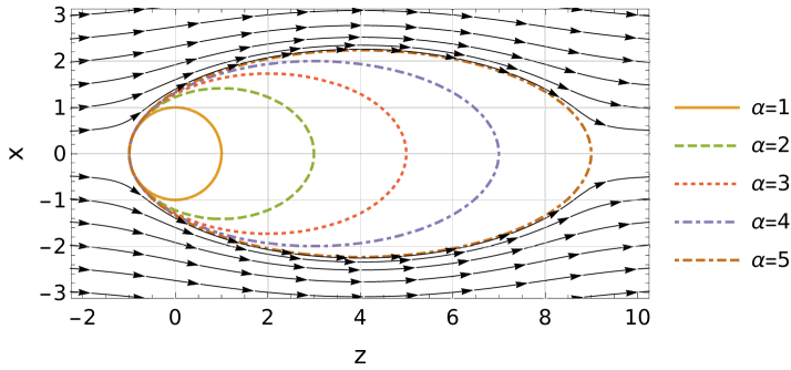
Figure 4: Different spheroids of the form $\left(x^{2}+y^{2}\right)/\alpha+\left(z-1+\alpha\right)^{2}/\alpha^{2}=1$ in the $y=0$ plane, along with streamlines (black arrows) of an incompressible flow around the most prolate body. The bodies are shifted such that their nose overlaps with the unit sphere.

It has been suggested (Keshet & Naor, 2016) that the flow in front of an axisymmetric body is well approximated by the flow in front of a sphere, rescaled to give the same nose curvature. Consider general prolate or oblate spheroids of the form $\left(x^{2}+y^{2}\right)/\alpha+z^{2}/\alpha^{2}=1$, chosen to be axisymmetric along the $\hat{z}$, flow axis, and with unit curvature at the nose. We shift the $z$ coordinate such that the resulting spheroid overlaps with the unit sphere at the nose $z\to z+1-\alpha^{2}$. The pseudospectral code (details in §C) is modified to solve the flow around such spheroids.

Figure 4 demonstrates the shapes of a sphere ($\alpha=1$) and of four shifted prolate spheroids ($\alpha\in\{2,3,4,5\}$), along with the incompressible flow along the latter, most prolate case. Figure 5 shows both the incompressible (left panels) and the critical (right panels) flows in front of these bodies. The normalized velocity $u$ (upper panels) varies with $\alpha$, ${\mathcal{M}}_{\infty}$ (and slightly with $\gamma$, see figure 5d and 3). However, a nearly universal result is obtained for the scaled velocity

$$u_{r}^{\rm{universal}}(r)\equiv u_{r}^{(\alpha)}\left(r,\theta=0\right)/\left(r^{-1}+1\right)^{\alpha^{-1/4}}\,,$$ (50)

approximately insensitive to the Mach number, prolate body profile, and value of $\gamma$. For oblate spheroids ($\alpha<1$), the velocity does not scale to the universal curve.

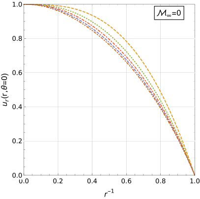
(a)

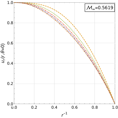
(b)

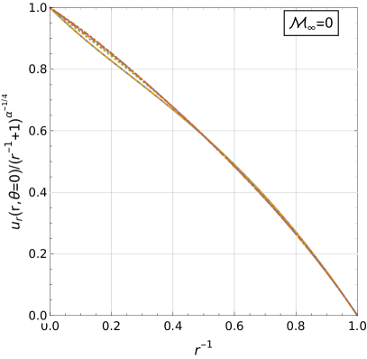
(c)

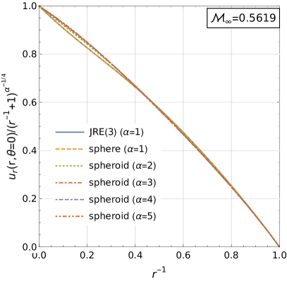
(d)

Figure 5: Incompressible (left panels) and critical (for the sphere: ${\mathcal{M}}_{\infty}=0.5619$; right panels) flows in front of the different spheroids of figure 4 (legend), showing the normalized velocity $u$ (upper panels) and the scaled velocity $u_{r}/\left(r^{-1}+1\right)^{\alpha^{-1/4}}$ (bottom panels). Results are based on the pseudospectral code with a converged, $\left(k_{\max},n_{\max}\right)=\left(8,8\right)$ resolution, for $\gamma=7/5$. In the bottom row we plot the third-order JRE around a sphere for comparison (JRE(3), solid blue).

8 Summary and discussion

We generalize the Janzen-Rayleigh expansion (JRE) of a hypersphere to arbitrary dimension, providing an exhaustive solution that supplements previous approaches with additional, usually necessary, logarithmic radial terms. Such a generalization is found to be essential in 3D, required for obtaining the correct solution for the sphere even at third ($m=3$, i.e. ${\mathcal{M}}_{\infty}^{6}$) order, although it is apparently not needed for the special case of a disk in 2D. The resulting, arbitrary-order JRE is a useful tool for studying various problems, as we demonstrate by generalizing and extending previous solutions for the axial flow of a sphere, and by presenting a simple approximate scaling that generalizes the axial flow for prolate spheroids.

The JRE of a potential, compressible flow is derived in general (in §2) and around a hypersphere of arbitrary dimension $d$ (in §3). The expansion is based on combining the continuity equation (4) and the Bernoulli equation (6) into a single equation (9) for the flow potential, $\phi$, which depends on the incident Mach number ${\mathcal{M}}_{\infty}$ far away from the hypersphere. An expansion of $\phi$ in powers of the ${\mathcal{M}}_{\infty}$ results in a set of recursive equations (2), with the zero order being the incompressible solution (20). The equations for higher orders, $\phi_{m}$, are derived as a sum of particular Poisson equations (37), with an exhaustive solution that is a finite sum (42) of terms combining powers of $r$, Jacobi polynomials ${\mathcal{J}}^{(d)}_{n}(\cos\theta)$, and, in addition, powers of $\ln{(r)}$ that emerge when the Poisson source terms satisfy one of the special conditions (38).

Previous JRE calculations were typically carried out with only part of the general solution, each order being considered as a sum of powers of $r$ and Jacobi polynomials alone. This approach works well in 2D, where one does not encounter any divergence when thus avoiding logarithmic terms, at least up to order $m=50$. However, this approach severely limits the JRE in 3D, as without logarithmic terms, the $m=3$ order diverges. The inclusion of logarithmic terms allows us to calculate terms much higher than available for any previous work in 3D (Kaplan, 1940; Tamada, 1940; Lighthill, 1960; Fuhs & Fuhs, 1976), and with higher accuracy (Frolov, 2003). Furthermore, we are able to compute the JRE to arbitrary order in any dimension, providing interesting insights on the flow. For instance, the JRE of the 4D hypersphere shows logarithmic terms at order $m=2$, indicating that the 3D sphere is not unique in requiring such terms.

After deriving the general solutions to all possible Poisson equations that can emerge in the problem (39, 40, and 41), we calculate the JRE analytically for general $\gamma$ to order $m=30$ in 2D and $m=18$ in 3D. For select values of $\gamma$, we proceed to compute $50$ JRE orders in 2D and $30$ orders in 3D.

The $m=3$ order JRE includes a $\gamma$-dependent logarithmic term proportional to $5+7\gamma+2\gamma^{2}$ (table 4), which does not vanish for $\gamma=1$ (i.e. $w=0$). This shows that both non-linear terms on the RHS of (2) contribute to the logarithm. We find that the highest order of any logarithmic term in the expansion increases by one every three orders in $m$, and when this occurs, only one logarithmic term appears, multiplied by a single power of $r$ and a single Legendre polynomial $\propto{r^{-2m-2}P_{2m+1}(\mu)}$ (see table 4 for $m=3$). We speculate that these findings are true for higher orders in the JRE and all physical values of $\gamma$ (conjecture 2).

We expect the absence of logarithmic terms in the 2D disk JRE to persist for all orders $m$ and for all $\gamma$ (conjecture 1). The absence of logarithmic terms is the disk JRE is not, however, a property of 2D flows in general. For instance, consider the incompressible flow of potential $\phi_{0}=(r+1/r)\cos\theta+B_{3}r^{-3}\cos(3\theta)$ around an algebraic body, which is defined by the no-slip BCs and this potential, unique in leading to a finite polynomial equation (Wallerstein & Keshet, in preparation). Here, $B_{3}$ is a coefficient in the general solution of the Laplace equation (18). The non-circular shape of the body leads to an infinite number of homogeneous terms in the first-order JRE potential $\phi_{1}$, and thus to an infinite number of both inhomogeneous and homogeneous terms in $\phi_{2}$. It is nevertheless possible to isolate the finite number of terms that contribute to the nonzero term $\propto{r^{-5}\cos(5\theta)\ln(r)}$ in $\phi_{2}$.

The absence of logarithmic terms in the disk JRE thus appears to indicate an additional symmetry unique to this 2D body. To illustrate this symmetry, consider how logarithmic terms could have putatively emerged in this JRE. The $m=0$ potential $\phi_{0}=(r+r^{-1})\cos\theta$ induces the $m=1$ Poisson source $2(r^{-7}-2r^{-5})\cos\theta+2r^{-3}\cos 3\theta$ in (2), none of which components satisfies (38), so $\phi_{1}$ has no logarithms. This source curiously lacks terms such as $r^{-5}\cos 3\theta$, which would have produced a logarithm in $\phi_{1}$. Such a ($k=-5$, $n=3$) term is conspicuously absent from the ($m=2$, $n=3$) Poisson source $[3r^{-11}-2(2+3\gamma)r^{-9}+18\gamma r^{-7}+19r^{-3}]\cos(3\theta)/6$. Inspecting (2), one sees several combinations $(m_{i},k_{i},n_{i})$ of terms among $\phi_{{m_{1}}}$, $\phi_{{m_{2}}}$, and $\phi_{{m_{3}}}$, each of which produces, in the $\phi_{2}$ source, a term

$${\scriptsize f\begin{pmatrix}m_{1}&k_{1}&n_{1}\\ m_{2}&k_{2}&n_{2}\\ m_{3}&k_{3}&n_{3}\end{pmatrix}}r^{-5}\cos 3\theta\,,$$ (51)

where $f$ are numerical coefficients. However, the sum of these coefficients vanishes,

$${\scriptsize f\begin{pmatrix}1&-3&1\\ 0&1&1\\ 0&1&1\end{pmatrix}}+{\scriptsize f\begin{pmatrix}0&-1&1\\ 0&1&1\\ 1&-1&1\end{pmatrix}}+{\scriptsize f\begin{pmatrix}0&-1&1\\ 1&-3&3\\ 0&1&1\end{pmatrix}}+{\scriptsize f\begin{pmatrix}0&1&1\\ 0&1&1\\ 1&-3&1\end{pmatrix}}$$ (52)

$$\quad\quad\quad+{\scriptsize f\begin{pmatrix}0&1&1\\ 1&-1&3\\ 0&1&1\end{pmatrix}}+{\scriptsize f\begin{pmatrix}0&-1&1\\ 0&-1&1\\ 1&-1&3\end{pmatrix}}=\frac{3}{2}-\frac{3}{4}+\frac{3}{2}-\frac{3}{4}-\frac{3}{4}-\frac{3}{4}=0\,,$$

leading to the absence of logarithms in $\phi_{2}$. Such a cancellation of terms persists at higher orders $m$.

Regardless of logarithmic terms, the angular part the solution includes Jacobi polynomials of odd $n$ for all JRE orders, so the flow is symmetric fore and aft of the hypersphere. Hence, as long as the JRE converges and no additional effects are included, there is no net force on the hypersphere, and the flow is drag-free for all dimensions. The d’Alembert paradox thus persists in all dimensions.

Even though we calculate the JRE to high orders, many physical features can be adequately captured with only a few low orders (figure 2), even for a sonic flows. For example, we find an accuracy better than $\sim 1\%$ in $\bm{u}$ for $m=5$. The low JRE orders ($m\leq 5$) show that compressibility effects are more prominent in the vicinity of the hypersphere, and in particular at the equatorial plane (figures 1 and 2).

With the ability to calculate the JRE to any desired accuracy, we compare it to other approximation methods, such as the hodographic approximation for the flow on the symmetry axis in front of a sphere, which has important physical implications even in the inviscid regime ( Keshet & Naor, 2016). The hodographic approximation of Keshet & Naor (2016) performs better than the JRE of order $m=0$, but worse than the JRE of order $m=1$ for any $\gamma$ (figure 3a and 3b). We use the JRE to improve the hodographic approximation (appendix §B), such that it performs better than JRE of order $m=2$, but worse than the JRE of order $m=3$ again for any $\gamma$, but can be continued to the supersonic regime (Keshet & Naor, 2016).

It has been speculated that the flow in front of the sphere can be applied to axisymmetric bodies with a similarly scaled nose curvature (Keshet & Naor, 2016, and references therein), such as prolate spheroids (figure 4). While the flows in front of different spheroids are not identical (figure 5a and 5b), they can be approximately mapped onto each other with a universal scaling, independent of $\gamma$ and ${\mathcal{M}}_{\infty}$, for flows ranging from the incompressible (figure 5c) to the sonic (5d) regimes. The velocity $u_{r}^{(\alpha)}$ in front of prolate spheroids with semi-axes $\alpha>0$ and $\alpha^{1/2}$ can be well approximated by a scaled JRE for a sphere

$$u_{r}^{(\alpha)}\left(r,\theta=0\right) \approx \left(r^{-1}+1\right)^{\alpha^{-1/4}-1}u_{r}^{(1)}\left(r,\theta=0\right)$$

$$\approx \left(r^{-1}+1\right)^{\alpha^{-1/4}-1}\sum\limits_{m=0}^{m_{max}}{\mathcal{M}}_{\infty}^{2m}\partial_{r}\phi_{m}\left(r,\theta=0\right).$$

It is natural to ask if such scalings can be identified using the generalized JRE in front of other bodies and in other dimensions, but this is beyond the scope of the present work.

We thank Y. Lyubarsky, D. Kogan and E. Grosfeld for helpful discussions. This research has received funding from the GIF (Grant No. I-1362-303.7 / 2016), and was supported by the Ministry of Science, Technology & Space, Israel, by the IAEC-UPBC joint research foundation (Grants No. 257/14 and 300/18), and by the Israel Science Foundation (Grant No. 1769/15).

Appendix A Explicit JRE coefficients for low orders

$a_{m,k,n}$	$m=0$	$m=1$		$m=2$			$m=3$
	$n=1$	$n=1$	$n=3$	$n=1$	$n=3$	$n=5$	$n=1$	$n=3$	$n=5$	$n=7$
$k=+1$	$1$
$k=-1$	$1$	$\frac{13}{12}$	$-\frac{1}{4}$	$\frac{17\gamma}{60}+\frac{343}{240}$	$-\frac{19}{48}$	$\frac{1}{16}$	$\frac{59\gamma^{2}}{420}+\frac{41\gamma}{42}+\frac{2273}{1120}$	$-\frac{17\gamma}{240}-\frac{137}{240}$	$\frac{25}{192}$	$-\frac{1}{64}$
$k=-3$		$-\frac{1}{2}$	$\frac{1}{12}$	$-\frac{\gamma}{8}-\frac{29}{24}$	$\frac{3}{20}-\frac{61\gamma}{240}$	$\frac{\gamma}{16}$	$-\frac{163\gamma}{240}-\frac{1759}{720}$	$-\frac{29\gamma^{2}}{210}-\frac{2117\gamma}{2100}+\frac{583}{14400}$	$\frac{97\gamma}{240}+\frac{157}{960}$	$-\frac{\gamma}{16}-\frac{1}{32}$
$k=-5$		$\frac{1}{12}$		$\frac{\gamma}{12}+\frac{35}{48}$	$\frac{3\gamma}{16}$	$-\frac{3\gamma}{80}-\frac{1}{80}$	$\frac{\gamma^{2}}{48}+\frac{47\gamma}{64}+\frac{3719}{1440}$	$\frac{\gamma^{2}}{16}+\frac{387\gamma}{320}+\frac{209}{960}$	$\frac{169\gamma^{2}}{1680}-\frac{11131\gamma}{33600}-\frac{60911}{302400}$	$-\frac{\gamma^{2}}{48}+\frac{7\gamma}{192}+\frac{5}{192}$
$k=-7$				$-\frac{\gamma}{16}-\frac{1}{4}$	$-\frac{\gamma}{40}-\frac{1}{60}$		$-\frac{\gamma^{2}}{16}-\frac{749\gamma}{960}-\frac{5443}{2880}$	$-\frac{\gamma^{2}}{40}-\frac{1493\gamma}{2400}-\frac{349}{1800}$	$-\frac{\gamma^{2}}{12}+\frac{\gamma}{16}+\frac{7}{96}$	$\frac{5\gamma^{2}}{336}+\frac{\gamma}{1344}-\frac{1}{336}$
$k=-9$				$\frac{\gamma}{80}+\frac{1}{30}$	$\frac{1}{144}$		$\frac{3\gamma^{2}}{80}+\frac{149\gamma}{320}+\frac{2449}{2880}$	$\frac{\gamma^{2}}{24}+\frac{281\gamma}{1440}+\frac{143}{1080}$	$\frac{\gamma^{2}}{112}+\frac{13\gamma}{2240}-\frac{13}{840}$
$k=-11$							$-\frac{\gamma^{2}}{60}-\frac{17\gamma}{120}-\frac{61}{288}$	$-\frac{\gamma^{2}}{112}-\frac{83\gamma}{2240}-\frac{5}{96}$	$\frac{1}{1440}-\frac{\gamma}{240}$
$k=-13$							$\frac{\gamma^{2}}{336}+\frac{113\gamma}{6720}+\frac{227}{10080}$	$\frac{\gamma}{240}+\frac{11}{1440}$	$\frac{1}{1728}$

Table 2: Coefficients table for the JRE up to third-order (${\mathcal{M}}_{\infty}^{6}$) in 2D (disk)

$b_{m,k,n,0}$	$m=0$	$m=1$		$m=2$			$m=3$
	$n=1$	$n=1$	$n=3$	$n=1$	$n=3$	$n=5$	$n=1$
$k=+1$	$1$
$k=-2$	$\frac{1}{2}$	$\frac{1}{3}$	$-\frac{3}{10}$	$\frac{599\gamma}{16800}+\frac{78733}{271040}$	$-\frac{53}{150}$	$\frac{5}{42}$	$\frac{131\gamma^{2}}{23520}+\frac{7507037\gamma}{100793000}+\frac{1160213239}{4192988800}$
$k=-4$			$\frac{27}{55}$		$\frac{83133\gamma}{3665200}+\frac{13691721}{19059040}$	$-\frac{6}{11}$
$k=-5$		$-\frac{1}{5}$	$-\frac{3}{10}$	$-\frac{3\gamma}{70}-\frac{149}{525}$	$-\frac{\gamma}{10}-\frac{23}{75}$	$\frac{\gamma}{7}+\frac{11}{21}$
$k=-5$							$-\frac{2519\gamma}{21000}-\frac{6013321}{15246000}$
$k=-6$						$\frac{4805247}{12172160}-\frac{50517\gamma}{276640}$
$k=-7$				$-\frac{243}{1925}$	$-\frac{156}{275}$	$-\frac{60}{77}$	$-\frac{4346757\gamma}{128282000}-\frac{457071093}{3335332000}$
$k=-8$		$\frac{1}{24}$	$\frac{3}{176}$	$\frac{\gamma}{24}+\frac{1381}{4620}$	$\frac{15\gamma}{176}+\frac{373}{880}$	$\frac{3\gamma}{52}+\frac{211}{728}$	$\frac{\gamma^{2}}{105}+\frac{50143\gamma}{246400}+\frac{26742953}{48787200}$
$k=-9$						$-\frac{3888}{21175}$
$k=-10$				$\frac{5589}{84700}$	$\frac{1137}{7150}$	$\frac{87}{1540}$	$\frac{573186051\gamma}{5644408000}+\frac{87731975043}{146754608000}$
$k=-11$				$-\frac{13\gamma}{560}-\frac{131}{924}$	$-\frac{57\gamma}{1960}-\frac{1075}{6468}$	$-\frac{9\gamma}{1120}-\frac{1697}{36960}$	$-\frac{17\gamma^{2}}{840}-\frac{179359\gamma}{646800}-\frac{1289}{1764}$
$k=-12$							$\frac{16281}{125125}$
$k=-13$							$-\frac{81\gamma}{1078}-\frac{355023}{770770}$
$k=-14$				$\frac{13\gamma}{2800}+\frac{6073}{369600}$	$\frac{23\gamma}{6800}+\frac{2957}{224400}$	$\frac{5\gamma}{8512}+\frac{1285}{561792}$	$\frac{43\gamma^{2}}{2800}+\frac{29644609\gamma}{153938400}+\frac{46207961}{92363040}$
$k=-16$							$\frac{33183\gamma}{1832600}+\frac{7173927}{104824720}$
$k=-17$							$-\frac{\gamma^{2}}{175}-\frac{7908301\gamma}{128282000}-\frac{3261710029}{25399836000}$
$k=-20$							$\frac{41\gamma^{2}}{47040}+\frac{2943929\gamma}{439824000}+\frac{2032133}{188496000}$

Table 3: Coefficients table for the third-order JRE (${\mathcal{M}}_{\infty}^{6}$) in 3D (sphere) (For the third-order only $n=1$ terms are present, see table 4 for the remaining terms)

$b_{m,k,n,0}$	$m=3$
	$n=3$	$n=5$	$n=7$
$k=-2$	$-\frac{599\gamma}{28000}-\frac{22815547}{60984000}$	$\frac{164}{819}$	$-\frac{35}{858}$
$k=-4$	$-\frac{418827051\gamma^{2}}{29673459200}+\frac{6207054461763\gamma}{73293444224000}+\frac{9236174319103493}{10480962524032000}$	$-\frac{9237\gamma}{366520}-\frac{157349}{146608}$	$\frac{567}{1573}$
$k=-5$	$-\frac{104327\gamma}{462000}-\frac{9833963}{30492000}$	$\frac{661\gamma}{1365}+\frac{4471}{4095}$	$-\frac{30\gamma}{143}-\frac{70}{143}$
$k=-6$		$-\frac{445149\gamma^{2}}{95190095}-\frac{587573895081\gamma}{1424043821200}+\frac{104968047599}{125190665600}$	$\frac{151551\gamma}{513760}-\frac{14415741}{22605440}$
$k=-7$	$-\frac{8118171\gamma}{50396500}-\frac{114716983}{100793000}$	$-\frac{1179657\gamma}{3335332}-\frac{55771}{46648}$	$\frac{756\gamma}{1573}+\frac{2916}{1573}$
$k=-8$	$\frac{61\gamma^{2}}{2420}+\frac{27461211\gamma}{70470400}+\frac{3347992607}{4651046400}$	$\frac{34\gamma^{2}}{1183}+\frac{2901\gamma}{47320}-\frac{4841}{141960}$	$\frac{427\gamma^{2}}{41184}-\frac{167888961127633\gamma}{166256455622400}-\frac{5482054296482347}{7315284047385600}$
$k=-9$	$\frac{16839\gamma}{304304}-\frac{1085826767}{3682078400}$	$\frac{33678\gamma}{112385}-\frac{4676251}{5439434}$	$\frac{1060857\gamma}{2825680}-\frac{1647800217}{1367629120}$
$k=-10$	$\frac{1149664413\gamma}{5241236000}+\frac{207885400509}{136272136000}$	$\frac{466297149\gamma}{1334132800}+\frac{4846089009}{2668265600}$	$\frac{12555\gamma}{53482}+\frac{131139}{106964}$
$k=-11$	$-\frac{361\gamma^{2}}{10780}-\frac{3681043\gamma}{8408400}-\frac{19239877}{18498480}$	$-\frac{19\gamma^{2}}{560}-\frac{18280747\gamma}{54654600}-\frac{24731363}{36436400}$	$-\frac{\gamma^{2}}{66}-\frac{16589\gamma}{111540}-\frac{125003}{408980}$
$k=-12$	$\frac{30359621107}{147283136000}-\frac{488331\gamma}{12172160}$	$\frac{36101964719}{118362083840}-\frac{18202959\gamma}{244549760}$	$\frac{44618931927}{415759252480}-\frac{20762487\gamma}{859006720}$
$k=-13$	$-\frac{147\gamma}{968}-\frac{646183}{692120}$	$-\frac{9861\gamma}{70070}-\frac{635053}{770770}$	$-\frac{2997\gamma}{78650}-\frac{192537}{865150}$
$k=-14$	$\frac{1803\gamma^{2}}{74800}+\frac{1337811833\gamma}{4596160800}+\frac{3982665971}{5515392960}$	$\frac{111\gamma^{2}}{6916}+\frac{1078190297\gamma}{5815249440}+\frac{3055176545}{6978299328}$	$\frac{57\gamma^{2}}{16016}+\frac{1873881\gamma}{45805760}+\frac{8865797}{91611520}$
$k=-16$	$\frac{31497\gamma}{919600}+\frac{6545551}{52601120}$	$\frac{26589\gamma}{1401400}+\frac{207773}{2802800}$	$\frac{3699\gamma}{1157728}+\frac{317763}{25470016}$
$k=-17$	$-\frac{17\gamma^{2}}{2200}-\frac{31358782537\gamma}{398333936000}-\frac{195575670263}{1195001808000}$	$-\frac{305\gamma^{2}}{88088}-\frac{21471961559\gamma}{613434261440}-\frac{136186343437}{1840302784320}$	$-\frac{7\gamma^{2}}{13728}-\frac{295271\gamma}{57383040}-\frac{623911}{57383040}$
$k=-20$	$\frac{553\gamma^{2}}{647680}+\frac{2385587089\gamma}{345181056000}+\frac{130642399631}{11390974848000}$	$\frac{281\gamma^{2}}{1019200}+\frac{501680027\gamma}{217273056000}+\frac{8141798513}{2048574528000}$	$\frac{5\gamma^{2}}{164736}+\frac{35015\gamma}{137719296}+\frac{1325845}{3029824512}$
$b_{m,k,n,1}$
$k=-8$			$-\frac{6\gamma^{2}}{143}-\frac{21\gamma}{143}-\frac{15}{143}$

Table 4: Coefficients table for the third-order JRE (${\mathcal{M}}_{\infty}^{6}$) in 3D (sphere) (only $n\in\{3,5,7\}$ terms). The last row indicates the single logarithmic term.

Expressions for the coefficients of the JRE up to order ${\mathcal{M}}_{\infty}^{6}$, valid for any $\gamma$, are provided in table 2 for a disk, and in tables 3 and 4 for a sphere. Each table is broken to parts, each corresponding to a different $m$ index of ${\mathcal{M}}_{\infty}^{2m}$. Columns correspond to the $n$ appearing in $\cos\left(n\theta\right)$ or $P_{n}\left(\cos\theta\right)$ basis functions, and the rows correspond to $k$ of the $r^{k}$ terms. All coefficients in these tables pertain to non-logarithmic terms, i.e. to $\propto\ln^{\ell}\left(r\right)$ terms with $\ell=0$, except for the very last term in table 4, which has $\ell=1$.

Appendix B Hodographic approximation of the solution of a radial flow

In §6 we discuss the hodographic approximation for the flow in front of a sphere, and use the JRE to obtain a more accurate expansion. To relate between the radial velocity and the radius we use Eq. (7) from Keshet & Naor (2016),

$$2\ln\left(r\right)={\int}_{0}^{-u_{r}(r)}\frac{1-{{\mathcal{M}}}_{0}{(u^{\prime})}^{2}/{W}^{2}}{1-{{\mathcal{M}}}_{0}{(u^{\prime})}^{2}/{S}^{2}}\frac{{du}^{\prime}}{q(u^{\prime})-u^{\prime}},$$ (54)

with $W^{2}=2/\left(\gamma+1\right),S^{2}=2/\left(\gamma-1\right)$ (notice that $S^{2}=w^{-1}$) and

$${\mathcal{M}}_{0}\left(u\right)=u/\overline{c}=u/\left(S^{-2}+{\mathcal{M}}_{\infty}^{-2}\right)^{1/2},$$

which is the Mach number with respect to the stagnation point. To complete the integral we calculate the coefficients $q_{i}$ for $i\in\{0,1,2,3\}$ using the JRE.

We provide explicit expressions for general $\gamma$ in table 5 which are valid for $0\leq{\mathcal{M}}_{\infty}\leq{\mathcal{M}}_{c}$ (with $q_{1}\equiv 1/2$ identically (Keshet & Naor, 2016)). These values give a good approximation for the radial velocity near the stagnation point, but deviates far from the sphere. To ensure the correct BC far from the body we add a fifth term to $q\left(u\right)$ such that the denominator in the integral in (54) vanishes at $r\to\infty$ i.e. $q_{4}=1-q_{0}-q_{1}-q_{2}-q_{3}$.

	$m=0$	$m=1$	$m=2$
$q_{0}$	$\frac{3}{2}$	$\frac{3}{2}-\frac{83{\mathcal{M}}_{\infty}^{2}}{220}$	$\frac{3}{2}-\frac{83{\mathcal{M}}_{\infty}^{2}}{220}-\frac{(378591917\gamma-678984653){\mathcal{M}}_{\infty}^{4}}{5690484800}$
$q_{2}$	$0$	$\frac{-1408394988000{\mathcal{M}}_{\infty}^{2}\left[{\mathcal{M}}_{\infty}^{2}(102855\gamma-333287)-3527160\right]}{\left[(378591917\gamma-678984653){\mathcal{M}}_{\infty}^{4}-2146864720{\mathcal{M}}_{\infty}^{2}+8535727200\right]^{2}}$	$\frac{-1408394988000{\mathcal{M}}_{\infty}^{2}\left[{\mathcal{M}}_{\infty}^{2}(102855\gamma-333287)-3527160\right]}{\left[(378591917\gamma-678984653){\mathcal{M}}_{\infty}^{4}-2146864720{\mathcal{M}}_{\infty}^{2}+8535727200\right]^{2}}$
$q_{3}$	$0$	$-\frac{7623000{\mathcal{M}}_{\infty}^{2}}{\left(83{\mathcal{M}}_{\infty}^{2}-330\right)^{3}}$	$\frac{-8014450271610182400000{\mathcal{M}}_{\infty}^{2}\left[{\mathcal{M}}_{\infty}^{2}(6569315\gamma+2958729)-16460080\right]}{\left[(378591917\gamma-678984653){\mathcal{M}}_{\infty}^{4}-2146864720{\mathcal{M}}_{\infty}^{2}+8535727200\right]^{3}}$

	$m=3$
$q_{0}$	$\frac{3}{2}-\frac{83{\mathcal{M}}_{\infty}^{2}}{220}+\frac{(378591917\gamma-678984653){\mathcal{M}}_{\infty}^{4}}{5690484800}-\frac{\left(1058753493922135\gamma^{2}-1417255351884097\gamma+1844488552375516\right){\mathcal{M}}_{\infty}^{6}}{37338428991864000}$
$q_{2}$	$\frac{2940401283109290000{\mathcal{M}}_{\infty}^{2}\left[\left(3584503350615\gamma^{2}+3753496299366\gamma-1602354228496\right){\mathcal{M}}_{\infty}^{4}-20622030(102855\gamma-333287){\mathcal{M}}_{\infty}^{2}+72737199334800\right]}{\left[\left(1058753493922135\gamma^{2}-1417255351884097\gamma+1844488552375516\right){\mathcal{M}}_{\infty}^{6}-6561555(378591917\gamma-678984653){\mathcal{M}}_{\infty}^{4}+14086770937839600{\mathcal{M}}_{\infty}^{2}-56007643487796000\right]^{2}}$
$q_{3}$	$\frac{-54894982258481009533016408280000000{\mathcal{M}}_{\infty}^{2}\left[\left(140520538815030\gamma^{2}+13019275653153\gamma-97154441684485\right){\mathcal{M}}_{\infty}^{4}-41244060(6569315\gamma+2958729){\mathcal{M}}_{\infty}^{2}+678880527124800\right]}{\left[\left(1058753493922135\gamma^{2}-1417255351884097\gamma+1844488552375516\right){\mathcal{M}}_{\infty}^{6}-6561555(378591917\gamma-678984653){\mathcal{M}}_{\infty}^{4}+14086770937839600{\mathcal{M}}_{\infty}^{2}-56007643487796000\right]^{3}}$

	$m=4$
$q_{0}$	$\begin{array}[]{ll}\frac{3}{2}-\frac{83{\mathcal{M}}_{\infty}^{2}}{220}+\frac{(378591917\gamma-678984653){\mathcal{M}}_{\infty}^{4}}{5690484800}-\frac{\left(1058753493922135\gamma^{2}-1417255351884097\gamma+1844488552375516\right){\mathcal{M}}_{\infty}^{6}}{37338428991864000}\\ +\frac{\left(14976238371862724157681480000\gamma^{3}-54767356061541106493910208468\gamma^{2}+21478489284009300130011513435\gamma-44582394863079130273355228987\right){\mathcal{M}}_{\infty}^{8}}{\left(1677449450721507819395719680000\right)}\end{array}$
$q_{2}$	$\begin{array}[]{l}-528396576977274963109651699200000{\mathcal{M}}_{\infty}^{2}\left[\left(113812743442673525009760\gamma^{3}-31571183798299137750086120\gamma^{2}-55929937306277740962895557\gamma\right.\right.\\ \left.\left.+20271206182723906597304662\right){\mathcal{M}}_{\infty}^{6}-11231387447280\left(3584503350615\gamma^{2}+3753496299366\gamma-1602354228496\right){\mathcal{M}}_{\infty}^{4}+231614008879431578400(102855\gamma\right.\\ \left.-333287){\mathcal{M}}_{\infty}^{2}-816939667559175886069344000\right]/\left[\left(14976238371862724157681480000\gamma^{3}-54767356061541106493910208468\gamma^{2}\right.\right.\\ \left.\left.+21478489284009300130011513435\gamma-44582394863079130273355228987\right){\mathcal{M}}_{\infty}^{8}-44925549789120\left(1058753493922135\gamma^{2}-1417255351884097\gamma\right.\right.\\ \left.\left.+1844488552375516\right){\mathcal{M}}_{\infty}^{6}+294781465846549281600(378591917\gamma-678984653){\mathcal{M}}_{\infty}^{4}-632855929135841586408385152000{\mathcal{M}}_{\infty}^{2}\right.\\ \left.+2516174176082261729093579520000\right]^{2}\end{array}$
$q_{3}$	$\begin{array}[]{l}-295452849271218270466030576021899437004399740039626752000000000{\mathcal{M}}_{\infty}^{2}\left[\left(1123633481124194863920377280\gamma^{3}-661946767058409457239821580\gamma^{2}\right.\right.\\ \left.\left.-1086310516712608715079428631\gamma+804276831488604048889927246\right){\mathcal{M}}_{\infty}^{6}-16847081170920\left(140520538815030\gamma^{2}+13019275653153\gamma-97154441684485\right){\mathcal{M}}_{\infty}^{4}\right.\\ \left.+694842026638294735200(6569315\gamma+2958729){\mathcal{M}}_{\infty}^{2}-11437155345828462404970816000\right]/\left[\left(14976238371862724157681480000\gamma^{3}\right.\right.\\ \left.\left.-54767356061541106493910208468\gamma^{2}+21478489284009300130011513435\gamma-44582394863079130273355228987\right){\mathcal{M}}_{\infty}^{8}-44925549789120\left(1058753493922135\gamma^{2}\right.\right.\\ \left.\left.-1417255351884097\gamma+1844488552375516\right){\mathcal{M}}_{\infty}^{6}+294781465846549281600(378591917\gamma-678984653){\mathcal{M}}_{\infty}^{4}-632855929135841586408385152000{\mathcal{M}}_{\infty}^{2}\right.\\ \left.+2516174176082261729093579520000\right]^{3}\end{array}$

Table 5: Coefficients of the first four terms in the Taylor expansion of $q\left(u\right)$, for different JRE orders $m$, at general Mach number and $\gamma$.

Appendix C Details and convergence of the pseudospectral solver

In order to capture the behaviour of the flow far and near the sphere (we review the implementation for the 3D case. The 2D case is similar with a difference only in the differential operators) we map the radial domain from $r\in[1,\infty]$ to $\varrho=r^{-1}\in[0,1]$. The differential operators with respect to $\varrho$ are

$$\bnabla_{\varrho}=\left(-\varrho^{2}\partial_{\varrho},\varrho\partial_{\theta}\right)\quad\mbox{and}\quad\nabla^{2}_{\varrho}=\varrho^{4}\partial_{\varrho\varrho}+\varrho^{2}\cot{\left(\theta\right)}\partial_{\theta}+\varrho^{2}\partial_{\theta\theta}.$$ (55)

The pseudospectral method requires the expansion of the solution as a series of functions (Boyd, 2001) (not required to be orthogonal) and evaluating the equation at collocation points. To ensure the polar BCs (no polar velocity on the poles i.e. Neumann BC for 3D and periodic boundary in 2D) we expand in cosine functions only, furthermore, the back and front reflection symmetry of the sphere limits the cosine functions to only odd cosines (as analytically shown for the JRE in §3), $\cos\left[\left(2n+1\right)\theta\right]$. In the radial direction we use the Chebyshev polynomials of the first kind (49). We take the collocation points to be

$$\varrho_{i}=\cos\left(\frac{\pi i}{2k_{max}}\right),\;1\leq i\leq k_{max}-1;\quad\theta_{j}=\frac{\pi j}{2\left(n_{max}+2\right)},\;1\leq j\leq n_{max}+1.$$ (56)

We do not consider the collocation points $\theta\in\{0,1\}$ because the expansion in odd cosines fulfills the BCs identically. On the points $\varrho\in\{0,1\}$ we solve the BCs at infinity and at the sphere respectively and not the non-linear equation (9). To solve the non-linear equation we use a simple Newton-Raphson algorithm where at each step we solve a linear set of equations. In all computation we take the error to be the maximal deviation of the equation at the collocation points and take a tolerance of $10^{-11}$. Most of the computations converge rapidly and do not require more than seven Newton-Raphson steps.

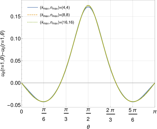
Figure 6: Compressibility contribution to the polar velocity on the sphere for different resolutions of the pseudospectral code at ${\mathcal{M}}_{\infty}=0.5619$ and $\gamma=7/5$.

Figure 6 shows the compressible contribution to the polar velocity on the sphere for various resolutions of the pseudospectral code. The code is quite converged, for most angles, except close to the equator and poles. A resolution of four by four shows the largest relative error (with respect to resolution of 16 by 32), which is smaller than $2\%$ at the equator. To test the robustness of the computation, we expand the solution with different functions, e.g. odd and even cosines as well as in sine functions, this resulted in the vanishing coefficient of the even cosine and sine functions. For the radial functions we expand in a linear combination of Chebyshev polynomials which fulfills the BC identically and in Legendre polynomials. All combinations gave the same results with respect to the tolerance.

We modify the code for the calculation of a compressible flow around spheroids of the form $\left(x^{2}+y^{2}\right)/\alpha+z^{2}/\alpha^{2}=1$. We use the prolate spheroidal coordinates, $\mu,\nu$ defined by

$$x=\sqrt{\alpha^{2}-\alpha}\cosh{(\mu)}\cos{(\nu)}\quad\mbox{and}\quad z=\sqrt{\alpha^{2}-\alpha}\sinh{(\mu)}\sin{(\nu)}\,.$$ (57)

(we omit the azimutal coordinate $\varphi$ from symmetry considerations). In this set of coordinates the body is described by the equation $\cosh(\mu_{b})=\sqrt{\alpha/(\alpha-1)}$. We normalize this coordinate and inverse it such that the computational domain is $[0,1]\times[0,\pi/2]$ just as in the case of the sphere. This changes the differential operators to (after variable change $\mu=\mu_{b}\varrho^{-1}$):

$$\bnabla_{\varrho}^{(\alpha)} = \frac{1}{\sqrt{\left(\alpha^{2}-\alpha\right)\left[\sinh^{2}\left(\mu_{b}\varrho^{-1}\right)+\sin^{2}\left(\nu\right)\right]}}\left(-\varrho^{2}\mu_{b}^{-1}\partial_{\varrho},\partial_{\nu}\right)\quad\mbox{and}\quad$$

$$\nabla^{2,(\alpha)}_{\varrho} = \frac{1}{\left(\alpha^{2}-\alpha\right)\left[\sinh^{2}\left(\mu_{b}\varrho^{-1}\right)+\sin^{2}\left(\nu\right)\right]}\left[\mu_{b}^{-2}\left(\varrho^{4}\partial_{\varrho\varrho}+2\varrho^{3}\partial_{\varrho}\right)-\varrho^{2}\mu_{b}^{-1}\coth\left(\mu_{b}\varrho^{-1}\right)\partial_{\varrho}\right.$$ (58)

$$\left.+\partial_{\nu\nu}+\cot\left(\nu\right)\partial_{\nu}\right].$$

We take $\phi_{0}$ to be a function that fulfills both BCs

$$\phi_{0}^{(\alpha)}=\left(\sqrt{\alpha^{2}-\alpha}\cosh\left(\mu_{b}\varrho^{-1}\right)+\sqrt{\alpha}\varrho\mu_{b}\right)\cos\left(\nu\right).$$ (59)

References

• Boyd (2001) Boyd, John P 2001 Chebyshev and Fourier spectral methods. Courier Corporation.
• Cecil et al. (2015) Cecil, Orie M., Majdalani, Joseph & Batterson, Joshua W. 2015 On steady trkalian high speed flows: Swirling compressible motions in rockets with headwall injection. 51st AIAA/SAE/ASEE Joint Propulsion Conference pp. AIAA 2015–3788.
• Chaggara & Koepf (2010) Chaggara, Hamza & Koepf, Wolfram 2010 On linearization coefficients of jacobi polynomials. Applied Mathematics Letters 23 (5), 609 – 614.
• Crowdy & Krishnamurthy (2018) Crowdy, Darren G. & Krishnamurthy, Vikas S. 2018 The effect of core size on the speed of compressible hollow vortex streets. Journal of Fluid Mechanics 836, 797–827.
• Feng et al. (2011) Feng, Jing-Jing, Huang, Ling & Yang, Shi-Jie 2011 Solutions of laplace equation in n-dimensional spaces. Communications in Theoretical Physics 56 (4), 623–625.
• Ferrari (1966) Ferrari, Carlo 1966 On the transonic controversy. Meccanica 1 (1-2), 37–44.
• Frolov (2003) Frolov, Vladimir 2003 High-speed compressible flows about axisymmetric bodies. In Fifth International Symposium on Cavitation (Cav2003).
• Fuhs & Fuhs (1976) Fuhs, Allen, E. & Fuhs, Susan, E. 1976 Phase distortion due to airflow over a hemispherical laser turret.
• Goldstein & Lighthillm (1944) Goldstein & Lighthillm 1944 Lxiii. two-dimensional compressible flow past a solid body in unlimited fluid or symmetrically placed in a channel. The London, Edinburgh, and Dublin Philosophical Magazine and Journal of Science 35 (247), 549–568.
• Green (2011) Green, D. A. 2011 A colour scheme for the display of astronomical intensity images. Bulletin of the Astronomical Society of India 39, 289–295, arXiv: 1108.5083.
• Guttmann & Thompson (1993) Guttmann, A. J. & Thompson, C. J. 1993 Subsonic potential flow and the transonic controversy. SIAM Journal on Applied Mathematics 53 (1), 48–59.
• Hasimoto (1951) Hasimoto, Hidenori 1951 On the subsonic flow of a compressible fluid past a rankine ovoid. Journal of the Physical Society of Japan 6 (3), 175–178, arXiv: https://doi.org/10.1143/JPSJ.6.175.
• Hida (1953) Hida, Kinzō 1953 On the subsonic flow of a compressible fluid past a prolate spheroid. Journal of the Physical Society of Japan 8 (2), 257–264, arXiv: https://doi.org/10.1143/JPSJ.8.257.
• Imai (1957) Imai, Isao 1957 Application of the m2-expansion method to compressible flow past isolated and lattice aerofoils. Journal of the Physical Society of Japan 12 (1), 58–67.
• Janzen (1913) Janzen, O. 1913 Beitrag zu einer theorie der stationären strömung kompressibler flüssigkeiten. Phys. Zeits 14 (1), 639–643.
• Kaplan (1940) Kaplan, Carl 1940 The flow of a compressible fluid past a sphere. Tech. Rep.. DTIC Document.
• Kaplan (1957) Kaplan, Carl 1957 On subsonic flow past a paraboloid of revolution. Tech. Rep.. University of North Texas Libraries, UNT Digital Library, Government Documents Department.
• Keshet & Naor (2016) Keshet, Uri & Naor, Yossi 2016 Compressible flow in front of an axisymmetric blunt object: analytic approximation and astrophysical implications. The Astrophysical Journal 830 (2), 147.
• Landau & Lifshitz (1959) Landau, L. D. & Lifshitz, E. M. 1959 Fluid mechanics. Butterworth-Heinemann.
• Leppington (2006) Leppington, F. G. 2006 The field due to a pair of line vortices in a compressible fluid. Journal of Fluid Mechanics 559, 45–55.
• Lighthill (1960) Lighthill, M. J. 1960 Higher Approximations in Aerodynamic Theory. Princeton University Press.
• Longhorn (1954) Longhorn, A. L. 1954 Subsonic compressible flow past bluff bodies. Aeronautical Quarterly 5 (3), 144–162.
• Maicke & Majdalani (2008) Maicke, Brian A. & Majdalani, Joseph 2008 On the rotational compressible taylor flow in injection-driven porous chambers. Journal of Fluid Mechanics 603, 391–411.
• Maicke et al. (2010) Maicke, B. A., Saad, T. & Majdalani, J. 2010 On the compressible hart-mcclure mean flow motion in simulated rocket motors. 46th AIAA/SAE/ASEE Joint Propulsion Conference pp. AIAA 2010–7077.
• Majdalani (2007) Majdalani, Joseph 2007 On steady rotational high speed flows: the compressible taylor–culick profile. Proceedings of the Royal Society A: Mathematical, Physical and Engineering Sciences 463 (2077), 131–162.
• Meiron et al. (2000) Meiron, D. I., Moore, D. W. & Pullin, D. I. 2000 On steady compressible flows with compact vorticity; the compressible stuart vortex. Journal of Fluid Mechanics 409, 29–49.
• Moon (2013) Moon, Young J. 2013 Sound of fluids at low mach numbers. European Journal of Mechanics - B/Fluids 40, 50 – 63, fascinating Fluid Mechanics: 100-Year Anniversary of the Institute of Aerodynamics, RWTH Aachen University.
• Moore & Pullin (1991) Moore, D. W. & Pullin, D. I. 1991 The effect of heat addition on slightly compressible flow: The example of vortex pair motion. Physics of Fluids A: Fluid Dynamics 3 (8), 1907–1914.
• Moore & Pullin (1998) Moore, D. W. & Pullin, D. I. 1998 On steady compressible flows with compact vorticity; the compressible hill’s spherical vortex. Journal of Fluid Mechanics 374, 285–303.
• Pham et al. (2005) Pham, Chi-Tuong, Nore, Caroline & Étienne Brachet, Marc 2005 Boundary layers and emitted excitations in nonlinear schrödinger superflow past a disk. Physica D: Nonlinear Phenomena 210 (3), 203 – 226.
• Rayleigh (1916) Rayleigh, Lord 1916 I. on the flow of compressible fluid past an obstacle. Philosophical Magazine Series 6 32 (187), 1–6.
• Slimon et al. (2000) Slimon, Scot A., Soteriou, Marios C. & Davis, Donald W. 2000 Development of computational aeroacoustics equations for subsonic flows using a mach number expansion approach. Journal of Computational Physics 159 (2), 377 – 406.
• Tamada (1940) Tamada, KO 1940 Further studies on the flow of a compressible fluid past a sphere. Proceedings of the Physico-Mathematical Society of Japan. 3rd Series 22 (7), 519–525.
• Van Dyke & Guttmann (1983) Van Dyke, MD & Guttmann, AJ 1983 Subsonic potential flow past a circle and the transonic controversy. The Journal of the Australian Mathematical Society. Series B. Applied Mathematics 24 (03), 243–261.
• Van Dyke (1958) Van Dyke, M. D. 1958 The paraboloid of revolution in subsonic flow. Journal of Mathematics and Physics 37 (1-4), 38–51.