Invisible Perturbations: Physical Adversarial Examples
Exploiting the Rolling Shutter Effect

Abstract

Physical adversarial examples for camera-based computer vision have so far been achieved through visible artifacts — a sticker on a Stop sign, colorful borders around eyeglasses or a 3D printed object with a colorful texture. An implicit assumption here is that the perturbations must be visible so that a camera can sense them. By contrast, we contribute a procedure to generate, for the first time, physical adversarial examples that are invisible to human eyes. Rather than modifying the victim object with visible artifacts, we modify light that illuminates the object. We demonstrate how an attacker can craft a modulated light signal that adversarially illuminates a scene and causes targeted misclassifications on a state-of-the-art ImageNet deep learning model. Concretely, we exploit the radiometric rolling shutter effect in commodity cameras to create precise striping patterns that appear on images. To human eyes, it appears like the object is illuminated, but the camera creates an image with stripes that will cause ML models to output the attacker-desired classification. We conduct a range of simulation and physical experiments with LEDs, demonstrating targeted attack rates up to $84\%$.

1 Introduction

Recent work has established that deep learning models are susceptible to adversarial examples — manipulations to model inputs that are inconspicuous to humans but induce the models to produce attacker-desired outputs [36, 17, 11]. Early work in this space investigated digital adversarial examples where the attacker can manipulate the input vector, such as modifying pixel values directly in an image classification task. As deep learning has found increasing application in real-world systems like self-driving cars [26, 15, 31], UAVs [8, 30], and robots [38], the computer vision community has made great progress in understanding physical adversarial examples [14, 5, 34, 24, 10] because this attack modality is the most realistic in physical systems.

Existing physical attacks include adding stickers on Stop signs that make models output Speed limit instead [14], colorful patterns on eyeglass frames to trick face recognition [34], and 3D-printed objects with specific textures [6]. However, all existing works add artifacts to the object (such as sticker or color patterns) that are visible to a human. In this work, we generate adversarial perturbations on real-world objects that are invisible to human eyes, yet produce misclassifications. Our approach exploits the differences between human and machine vision to hide adversarial patterns.

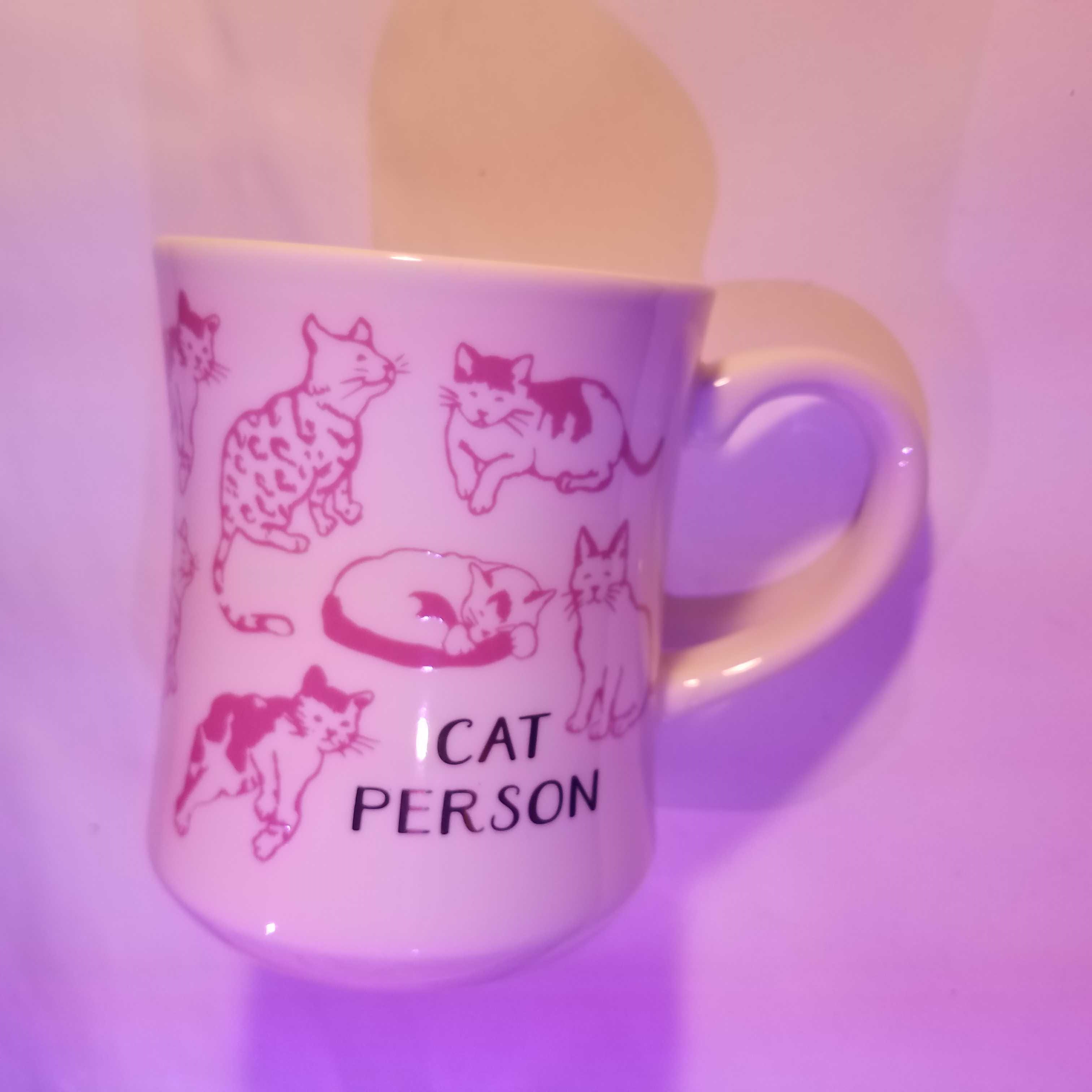
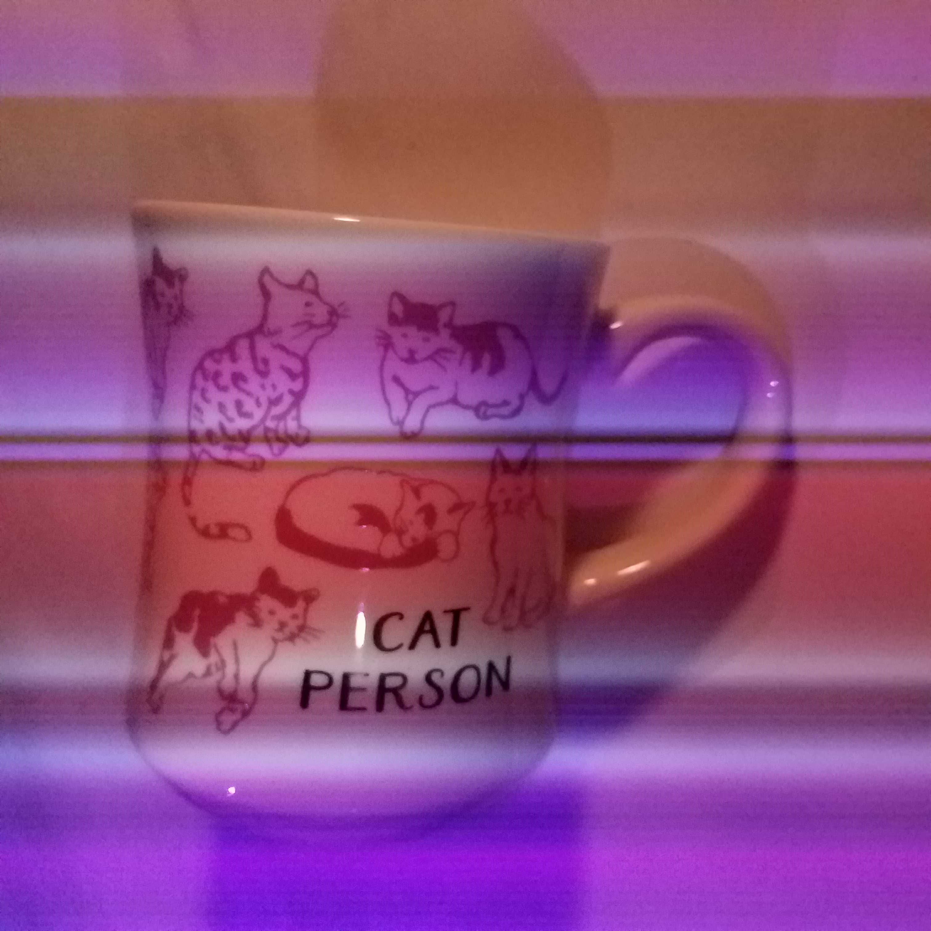
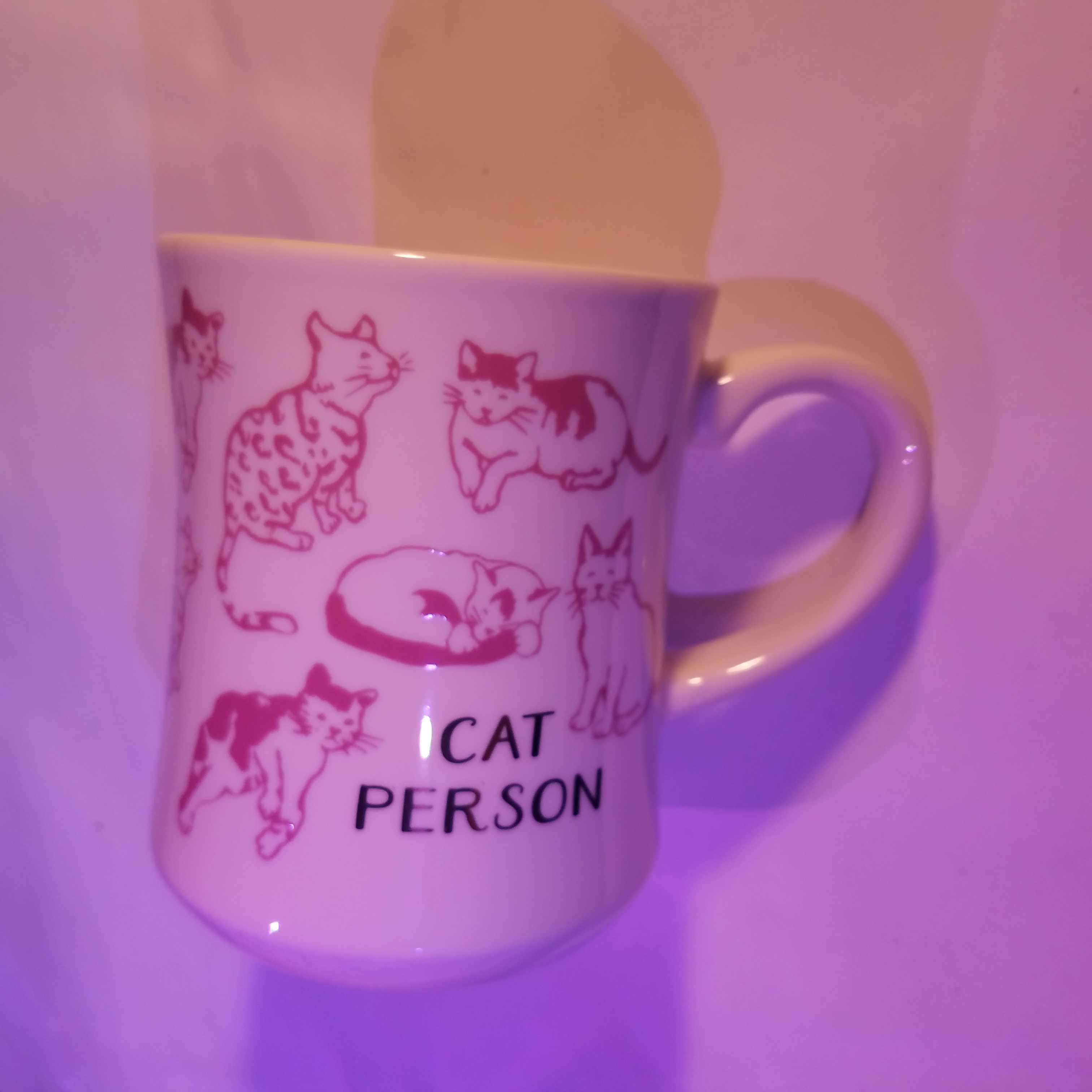
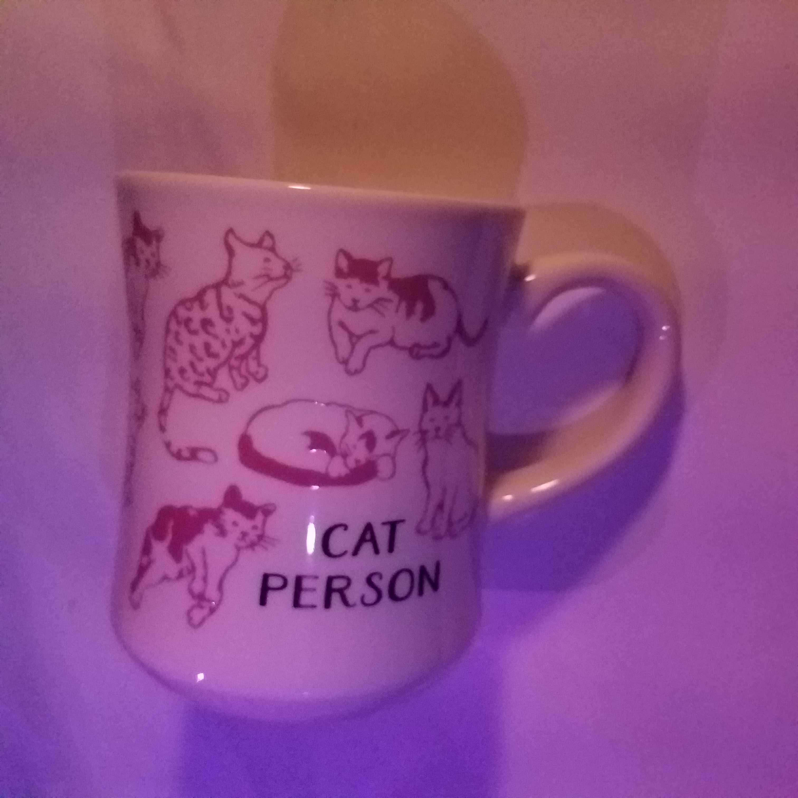
       With Attack Signal                       Without Attack Signal

Figure 1: Images as seen by human (without border) and as captured by camera (in black border) with the attack signal (left two images) and without (right two images). The image without the attack signal is classified as coffee mug (confidence $55\%$), while the image with the attack signal is classified as perfume (confidence $70\%$). The attack is robust to camera orientation, distance, and ambient lighting.

We show an invisible physical adversarial example in fig:teaser, generated by manipulating the light that shines on the object. The light creates adversarial patterns in the image that only a camera perceives. In particular, we show how an attacker can exploit the radiometric rolling shutter (RS) effect, a phenomenon that exists in rolling shutter cameras that perceive a scene whose illumination changes at a high frequency. Digital cameras use the rolling shutter technique to obtain high resolution images at higher rate and at a cheaper price [3, 27]. Rolling shutter technology is used in a majority of consumer-grade cameras, such as cellphones [19], AR glasses [32] and machine vision [1, 2].

Due to the rolling shutter effect, the adversarially-illuminated object results in an image that contains multi-colored stripes. We contribute an algorithm for creating a time-varying high-frequency light pattern that can create such stripes. To the best of our knowledge, this is the first demonstration of physical adversarial examples that exploit the radiometric rolling shutter effect, and thus, contributes to our evolving understanding of physical attacks on deep learning camera-based computer vision.

Similar to prior work on physical attacks, the main challenge is obtaining robustness to dynamic environmental conditions such as viewpoint and lighting. However, in our setting, there are additional environmental conditions that pose challenges in creating these attacks. Specifically: (1) Camera exposure settings influence how much of the rolling shutter effect is present, which affects the attacker’s ability to craft adversarial examples. — long exposures lead to less pronounced rolling shutter, providing less control. (2) The attacker’s light signal can be de-synchronized with respect to the camera shutter, thus causing the camera to capture the adversarial signal at different offsets causing the striping pattern to appear at different locations on the image, that can destroy its adversarial property. (3) The space of possible perturbations is limited compared to existing attacks. Unlike sticker attacks or 3D objects that can change the victim object’s texture, our attack only permits striped patterns that contain a limited set of translucent colors. (4) Difference in the light produced by RGB LEDs and the color perceived by camera sensor makes it harder to realize a physical signal.

To tackle the above challenges, we create a simulation framework that captures these environmental and camera imaging conditions. The simulation is based on a differentiable analytical model of image formation and light signal transmission and reception when the radiometric rolling shutter effect is present. Using the analytical model, we then formulate an optimization objective that we can solve using standard gradient-based methods to compute an adversarial light signal that is robust to these unique environmental and camera imaging conditions. We fabricate this light signal using programmable LEDs.

Although light-based adversarial examples are limited in the types of perturbation patterns compared to sticker-based ones, they have several advantages: (1) The attack is stealthier than sticker-based ones, as the attacker can simply turn the light source to a constant value to turn OFF the attack. (2) Unlike prior work using sticker or 3D printed object, the perturbation is not visible to human eyes. (3) The attack is dynamic and can change on-the-fly — in a sticker-based attack, once the sticker has been placed, the attack effect cannot be changed unless the sticker is physically replaced. In our setting, the attacker can simply change the light signal and thus, change the adversarial effect.

We characterize this new style of invisible physical adversarial example using a state-of-the-art ResNet-101 classifier trained using ImageNet [13]. We conduct physical testing of our attack algorithm under various viewpoints, ambient lighting conditions, and camera exposure settings. For example, for the coffee mug shown in fig:teaser we obtain a targeted fooling rate of $84\%$under a variety of conditions. We find that the attack success rate is dependent on the camera exposure setting: exposure rates shorter than $1/750s$ produce the most successful and robust attacks.

The main contributions of our work are the following:

• We develop techniques to modulate visible light that can illuminate an object to cause misclassification on deep learning camera-based vision classifiers, while being completely invisible to humans. Our work contributes to a new class of physical adversarial examples that exploit the differences between human and machine vision.

• We develop a differentiable analytical model of image formation under the radiometric rolling shutter effect and formulate an adversarial objective function that can be solved using standard gradient descent methods.

• We instantiate the attack in a physical setting and characterize this new class of attack by studying the effects of camera optics and environmental conditions, such as camera orientation, lighting condition, and exposure. Code is available at https://github.com/EarlMadSec/invis-perturbations.

2 Related Work

Digital Adversarial Examples.

This type of attack has been relatively well-studied [36, 17, 11, 29, 33, 7, 22] with several attack techniques proposed. They all involve creating pixel-level changes to the image containing a target object. However, this level of access is not realistic when launching attacks on cyber-physical systems — an attacker who has the ability to manipulate pixels at a digital level already has privileged access to the system and can directly launch simpler attacks that are more effective. For example, the computer security community has shown how an attacker could directly (de)activate brakes in a car [21].

Physical Adversarial Examples.

Physical perturbations are the most realistic way to attack physical systems. Recent work has introduced attacks that require highly visible patterns affixed to the victim object, such as stickers/patches on traffic signs, patterned eyeglass frames or 3D printed objects [14, 6, 10, 37, 34]. We introduce a new kind of physical adversarial example that cameras can see but humans cannot. Li et al. [24] recently proposed adversarial camera stickers. These do not require visible stickers on the target object, but they require the attacker to place a sticker on the camera lens. By contrast, we target a more common and widely used threat model where the attacker can only modify the appearance of a victim object.

Rolling Shutter Distortions.

Broadly, rolling shutter can manifest in two kinds of image distortions: (1) motion-based, where the camera or object move during capture, and (2) radiometric, where the lighting varies rapidly during camera exposure. The more common among the two is motion-based, and thus, most prior work has examined techniques to correct motion distortions [3, 16, 12, 9]. Early works derived geometric models of rolling-shutter cameras and removed image distortions due to global, constant in-plane translation [16, 12], which was later extended to non-rigid motion via dense optical flow [9]. Our work focuses on exploiting radiometric distortions caused by high-frequency lights.

Rolling Shutter for Communication.

A line of work has explored visible light communication using the radiometric rolling shutter effect [18, 23]. Similar to our work, the goal is to transmit information from a light source to a camera by modulating a high-frequency time-varying light signal such as an LED. We take inspiration from this work and explore how an adversary can manipulate the light source to transmit an adversarial example. However, the key difference is that there is no “receiver” in our setting. Rather, the attacker must be able to transmit all information necessary for the attack in a single image without any co-operation from the camera. By contrast, the communication setting can involve taking multiple images over time because the light source and camera co-operate to achieve information transfer. In our case, the light signal must robustly encode information so that the attack effect is achieved in the span of a single image — a challenge that we address.

Rolling Shutter for Visual Privacy.

Zhu et al. [39] proposed using radiometric rolling shutter distortions to reduce the signal-to-noise ratio in an image until it becomes unintelligible to humans. This helps to prevent photography in sensitive spaces. Our goal is orthogonal — we wish to manipulate the rolling shutter effect to cause targeted misclassifications in deep learning models.

3 Image Formation under Rolling Shutter

Rolling Shutter Background.

Broadly, cameras are of two types depending on how they capture an image: (1) rolling shutter (RS) and (2) global shutter. A camera consists of an array of light sensors (each sensor corresponds to an image pixel). While an image is being formed, these sensors are exposed to light energy for a period of $t_{e}$, known as exposure time, and then the data is digitized and read out to memory. In a global shutter, the entire sensor array is exposed at the same time and then the sensors are turned off for the readout operation. By contrast, an RS camera exposes each row of pixels at slightly different periods of time. Thus, while rows are being exposed to light, the data for previously exposed rows are read out. This leads to a higher frame-rate than for high resolution cameras.

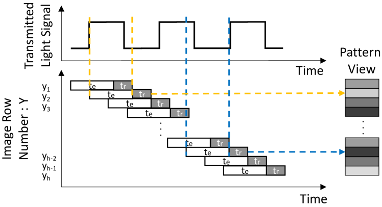
Figure 2: Modulated light induces the radiometric rolling shutter effect. Here $t_{r}$ denotes the time it takes to read a row of sensors, and $t_{e}$ denotes the exposure of the camera.

We visualize the rolling shutter effect in the presence of lighting changes in fig:rs. For an RS camera, the time it takes to read a row is called readout time ($t_{r}$). Each row is exposed and read out at a slightly later time than the previous row. Let $t_{0}$ be the time when the first row is exposed, then the $y^{\textit{th}}$ row is exposed at time $t_{0}+(y-1)t_{r}$, and read at $t_{0}+(y-1)t_{r}+t_{e}$.

As different rows are exposed at different points in time, any lighting or spatial changes in the scene that occurs while the image is being taken can lead to undesirable artifacts in the captured image, including distortion or horizontal stripes on the image, known as rolling shutter effect [25]. In this work, we exploit such artifacts by modulating a light source. We contribute a technique to determine the precise modulation required to trick state-of-the-art deep learning models for visual classification.

Image Formation.

We represent the time-modulated attacker signal as $f(t)$. We assume that the scene contains ambient light in addition to the attacker-controlled light source (e.g., a set of Smart LED lights). Let $l_{tex}(x,y)$ represent the texture of the scene, which we approximate as the value of the $(x,y)$ pixel. As the attacker signal is a function of time, the illumination at pixel $(x,y)$ on the scene will vary over time, $(\alpha+\beta\>f(t))$. Here $\alpha$ and $\beta$ represent the intensity of the ambient light and the maximum intensity of the attacker controlled light, respectively. We note that the attacker can use an RGB LED, and thus, the attacker’s signal contains three components: Red, Green and Blue.

In rolling shutter camera, pixels on the same row are exposed at the same time, and neighboring rows are exposed at slightly different times. Let each row be exposed for $t_{e}$ seconds, and the $y^{\textit{th}}$ row starts exposing at time $t_{y}$. Therefore, the intensity of a pixel $(x,y)$ in row $y$, will be: $i(x,y)=\rho\int_{t_{y}}^{t_{y}+t_{e}}l_{tex}(x,y)\>\left(\alpha+\beta\>f(t)\right)\>dt$. Here, $\rho$ denotes the sensor gain of the camera sensor that converts the light radiance falling on a pixel sensor into a pixel intensity. Thus, we have:

$$i(x,y) = \rho\>l_{tex}(x,y)\left(\alpha t_{e}+\beta\int_{t_{y}}^{t_{y}+t_{e}}f(t)\>dt\right)$$

$$= \rho\>l_{tex}(x,y)\>t_{e}\>\alpha+\rho\>l_{tex}(x,y)\>t_{e}\>\beta\>g(y)$$

$$= I_{\mathsf{amb}}+I_{\mathsf{sig}}\cdot g(y)$$

Here, the signal image $g(y)$ denotes the average effect of signal $f(t)$ on row $y$, $g(y)={1\over t_{e}}\int_{t_{y}}^{t_{y}+t_{e}}f(t)\>dt$. Let $I_{\mathsf{amb}}$ be the image captured under only ambient light, such that $I_{\mathsf{amb}}=\rho\>l_{tex}(x,y)t_{e}\alpha$, and $I_{\mathsf{sig}}$ is the image captured under only the full illumination of the attacker controlled light (with no ambient light).

The time-varying signal $f(t)$ we generate is periodic, with period $\tau$; during the image capture the signal could have an offset of $\delta$ with respect to the camera. Therefore, final equation of pixel intensity would be,

$$I_{\mathsf{fin}}=I_{\mathsf{amb}}+I_{\mathsf{sig}}\cdot g(y+\delta)$$ (1)

In the next section, we discuss how we make our attack robust to environmental conditions, including any offset $\delta$.

4 Crafting Invisible Perturbations

Our high-level goal is to generate a light signal by modulating a light source such that it induces striping patterns when a rolling shutter camera senses the scene. These patterns should be adversarial to a machine learning model but should not be visible to humans. The attacker light source flickers at a frequency that humans cannot perceive, and thus, the scene simply appears to be illuminated. fig:pipeline outlines the attack pipeline. To achieve this goal, we first present the challenges in crafting such light modulation, followed by our algorithm for overcoming these issues.

4.1 Physical World Challenges

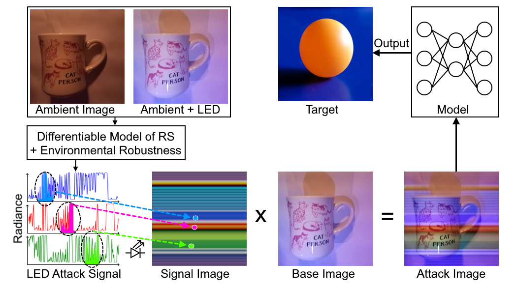
Figure 3: The attacker creates a time-modulated high frequency light signal that induces radiometric striping distortions in rolling shutter cameras. The striping pattern is designed to cause misclassifications.

One of the key challenges in creating physical adversarial examples is to create a simulation framework that can accurately estimate the final image taken by the camera. Without such a framework it will be very slow to compute an attack by repeating physical experiments. In addition, physical world perturbations must survive varying environmental conditions, such as viewpoint and lighting changes. Prior work has proposed methods that can create adversarial examples robust to these environmental factors. However, in our setting, we encounter a unique set of additional challenges concerning light generation, reception, and camera optics.

Desynchronization between camera and light source.

The location of the striping patterns appearing on the image depends on the synchronization between the camera and the light source. Failing to do so, will cyclically permute the striping pattern on the image, resulting in a different final image. However, the attacker has no control over the camera and when the image is taken. Therefore, we optimize our signal to remain adversarial even when the light source is out of sync with the camera at image capture time.

Camera exposure.

The exposure of the camera will significantly change how a particular attacker signal is interpreted. A long exposure will apply a “smoothing effect” on the signal as two consecutive rows will receive much of the same light. This will reduce the attacker’s ability to cause misclassifications. A shorter exposure would create more pronounced bands on the image, making it easier to induce misclassification. We show that our adversarial signal can be effective for a wide range of exposure values.

Color of light production and reception.

Prior work has examined fabrication error in the case of printer colors [14, 34]. Our attack occurs through an LED and this requires different techniques to account for fabrication errors: (1) Red, Green, Blue LEDs produce light of different intensities; (2) Cameras run proprietary color correction; (3) Transmitted light can bleed into all three color channels (e.g., if only Red light is transmitted, on the sensor side, it will still affect the Green and Blue channels). We learn approximate functions to translate a signal onto an image so that we can create a simulation framework for quickly finding adversarial examples.

4.2 Optimization Formulation

Our goal is to compute a light signal $f(t)$ such that, when an image is taken under the influence of this light signal, the loss is minimized between the model output and the desired target class. However, unlike prior formulations, we do not need an $\ell_{P}$ constraint on perturbation magnitude because our perturbations (via high-frequency light modulation) are invisible to human eyes by design. Instead, our formulation is constrained by the capabilities of the LEDs, the Arduino chip we use to modulate them (see sec:realize), and the camera parameters. A novel aspect in our formulation is the differentiable representation of the rolling shutter camera and color correction applied by the camera. Such representation allows us to compute the adversarial example end-to-end using common gradient-based methods, such as PGD [28] and FGSM [17]. Our model allows us to manipulate camera parameters such as exposure time, image size and row readout rate.

Following Eq. (1), we get the final image $I_{\mathsf{fin}}$ as a sum of the image in ambient light($I_{\mathsf{amb}}$) and in only the attacker’s light source($I_{\mathsf{sig}}$). Based on the image formation model discussed above, we have the following objective function:

$$\min_{f(t)}\>\mathop{\operatorname{\mathbb{E}}}_{\mathsf{C},\mathsf{T},\delta}J\left({\mathcal{M}}(\mathsf{C}(I_{\mathsf{fin}})),k\right)$$ (2)

$$I_{\mathsf{fin}}=\mathsf{T}\left(I_{\mathsf{amb}}\right)+\mathsf{T}\left(I_{\mathsf{sig}}\right)\cdot g(y+\delta)$$

$$g(y)={1\over t_{e}}\int_{t_{y}}^{t_{y}+t_{e}}f(t)\>dt$$

where $J(.,k)$ is the classification loss for the target class $k$, ${\mathcal{M}}$ is the classifier model, $\mathsf{C}$ is a function to account for color reproduction error, $\mathsf{T}$models viewpoint and lighting changes, $\delta$ denotes possible signal offsets. The image under only ambient light is $I_{\mathsf{amb}}$ and under only fully illuminated attacker-controlled light is $I_{\mathsf{sig}}$.

As we assume the attacker does not have control over the ambient light, we cannot take $I_{\mathsf{sig}}$ (image without the effect of the ambient light). We instead take an image where both ambient and the attacker controlled LEDs are fully illuminated, which we call $I_{\mathsf{full}}=I_{\mathsf{amb}}+I_{\mathsf{sig}}$, and extrapolate $I_{\mathsf{sig}}$ as $I_{\mathsf{full}}-I_{\mathsf{amb}}$.

The process of solving the above optimization problem is shown in Algorithm 1. We use the cross-entropy as our loss function $J$ and used ADAM [20] as the optimizer. Next, we discuss how our algorithm handles the unique challenges (subsec:phy-challenges) to generate robust adversarial signals.

Input: Image with only ambient light $I_{\mathsf{amb}}$, image with ambient and attacker controlled lights $I_{\mathsf{full}}$, target class $k$, and exposure value $t_{e}$
Output: Digitized adversarial light signal $\hat{f}$, which is an vector of size $l$.
Notations: $c$: number of color channels; $\mathsf{shift}(.,\delta)$: cyclic permutation of an vector shifted by $\delta$ places; $\gamma$: parameter for gamma correction; $N$: threshold for maximum number of iteration; $s$ is the shutter function which depends on the $t_{e}$ and image size $h\times w$

procedure OPTIMIZE($I_{\mathsf{amb}},I_{\mathsf{full}},k,s$)

    $n\leftarrow 1$

    $v_{0}{\>{\leftarrow{\raisebox{0.75pt}{$\scriptscriptstyle\$$}}}\>}\mathbb{Z}^{c\times l}$ $\triangleright$ Randomly sample an vector of size $c\times l$

    while not converge and $n\leq N$ do

        $\mathsf{C}\sim P,\mathsf{T}\sim X,\delta\sim\{0,1,\ldots,l\}$

        $\hat{f}_{n}\leftarrow\frac{1}{2}(\tanh(v_{n-1})+1)$

        $o_{n}\leftarrow$ $\mathsf{shift}(\hat{f}_{n},\delta)$ $\triangleright$ cyclic permutation

        $g_{n}\leftarrow o_{n}*s$ $\triangleright$ convolution with the shutter function

        $I_{\mathsf{amb},n}\leftarrow\mathsf{T}(I_{\mathsf{amb}});\;\;I_{\mathsf{full},n}\leftarrow\mathsf{T}(I_{\mathsf{full}})$

        $I_{\mathsf{sig},n}\leftarrow\left(I_{\mathsf{amb},n}^{\gamma}+g_{n}\times(I_{\mathsf{full},n}^{\gamma}-I_{\mathsf{amb},n}^{\gamma})\right)^{1\over\gamma}$

        $L\leftarrow J\left({\mathcal{M}}\left(\mathsf{C}(I_{\mathsf{sig},n})\right),k\right)$ $\triangleright$ loss for target class k

        $\Delta v\leftarrow\nabla_{v_{n-1}}L$

        $v_{n}\leftarrow v_{n-1}+\Delta v$

        $n\leftarrow n+1$

    end while

    $\hat{f}\leftarrow\frac{1}{2}(\tanh(v_{n})+1)$

    return $\hat{f}$

end procedure

Algorithm 1 Adversarial Light Signal Generation

Structure of $f(t)$.

One of the challenges in solving the above optimization problem is determining how to represent the time-vary attacker signal $f(t)$ in a suitable format. We choose to represent it as an vector of intensity values, which we denote as $\hat{f}$. Each index in $\hat{f}$ represents a time interval of $t_{r}$ (i.e., the readout time of the camera). This is because the attacker will not gain any additional control over the rolling shutter effect by changing the light intensity within a single $t_{r}$ period: Within a single $t_{r}$, the same set of rows are exposed to light and any intensity changes will be averaged. Furthermore, we bound the values of $\hat{f}$ to be in $[0,1]$, such that $0$ denotes zero intensity and $1$ denotes full intensity. The signal values inside are scaled accordingly. To ensure our signal is within the bounds, we use a change-of-variables. We define $\hat{f}=\frac{1}{2}(\tanh(v)+1)$. Thus, $v$ can take any unbounded value during our optimization. Finally, the attacker must determine what is an appropriate length of $\hat{f}$ because the optimizer needs a tensor of finite size. We design $\hat{f}$ to be periodic with period equal to image capture time: $t_{r}\cdot h+t_{e}$ where $h$ is the height of the image in pixels. As each index in $\hat{f}$ represents $t_{r}$ units of time, the length of the vector for $\hat{f}$ would be $l=h+\Bigl{\lceil}{{t_{e}}\over t_{r}}\Bigl{\rceil}$.

Viewpoint and Lighting Changes.

We build on prior work in obtaining robustness to viewpoint (object pose) and lighting variability. Specifically, we use the expectation-over-transformation approach (EoT) that samples differentiable image transformations from a distribution (E.g., rotations, translations, brightness) [6]. We model this using distribution $X$ which consists of transformations for flipping the image horizontally and vertically, magnifying the image to account for small distance variations, and planar rotations of the image. During each iteration of the optimization process, we sample a transformation $\mathsf{T}$ from $X$ and apply it to the pair of object images $I_{\mathsf{amb}}$ and $I_{\mathsf{full}}$. We apply multiplicative noise to the ambient light image $I_{\mathsf{amb}}$ to model small variations in the ambient light. However, to account for a wider variation in the ambient light, we adjust our signal during attack execution. This is one of the key benefits of this attack to be agile to environment changes. We generate a set of adversarial light signals, each designed to operate robustly at specific intervals of ambient light values. During the attack, we switch our light signal to the one that corresponds to the current ambient light setting. Using this approach, we avoid optimizing over large ranges of ambient light conditions and hence, improve the effectiveness of our attack.

Signal Offset.

Because our signal can have a phase difference with the camera, we account for this during optimization. The offset is an integer value $\delta\in\{0,1,\ldots,l\}$. Each offset value can be represented by a specific cyclic permutation of the $\hat{f}$ vector. A offset value of $\delta$ corresponds to performing a $\delta$-step cyclic rotation on the signal vector. To gain robustness against arbitrary offsets, we model the cyclic rotation as a matrix multiplication operation. This enables us to use EoT by sampling random offsets during optimization.

Color Production and Reception Errors.

Imperfections in light generation and image formation by the camera can lead to errors. Furthermore, the camera can run proprietary correction steps such as gamma correction to improve image quality. We account for the gamma correction by using the sRGB (Standard RGB) standard value, $\gamma=2.2$ [4]. However, it is infeasible to model all possible sources of imperfection. Instead, we model the fabrication error as a distribution of transformations in a coarse-grained manner and perform EoT to overcome the color discrepancy. The error transformations are a set of experimentally-determined affine ($Ax+B$) or polynomial ($a_{0}x^{n}+a_{1}x^{n-1}+...+a_{n}$) transformations applied per color channel (term $\mathsf{C}$ in Eq. (2)). Please see the supplementary material for exact parameter ranges for the distribution $P$ from which we sample $\mathsf{C}$ values.

Handling Different Exposures.

Eq. 2 models the effect of the attacker signal on the image as a convolution between $f(t)$ and a shutter function. Shorter exposure leads to smaller convolution sizes, and longer exposure leads to larger convolution size. Instead of optimizing for different exposure values, we take advantage of a feature of this new style of physical attack — its dynamism. Specifically, the attacker can optimize different signals $f(t)$ for different discrete exposure values and then, at attack execution, switch to the signal that is most appropriate to the camera being attacked and ambient light. As most cameras have standard exposure rates, the attacker can apriori create different signals. We note that dynamism is a feature of our work and is not possible with current physical attacks [14, 6, 24, 37, 34, 10].

5 Producing Attack Signal using LED lights

We used a simulation framework to generate adversarial light signals for a given scene and camera parameters. To validate that these signals are effective in the real world, we implement the attack using programmable LEDs. The primary challenge we address here is modulating an LED according to the optimized signal $\hat{f}$, a vector of reals in $[0,1]$.

We use an Arduino Atmel Cortex M-3 chip (clock rate $84$ MHz) to drive a pair of RGB LEDs. We used a Samsung Galaxy S7 for taking images, whose read out time ($t_{r}$) is around $10~{}\mu s$. The camera takes images at resolution $3024\times 3024$, which is $12$x larger than the input size that our algorithm requires $252\times 252$. Our optimization process resizes images to $224\times 224$ before passing to ResNet-101 classifier. Thus, when a full-resolution image is resized to the dimensions of the model, 12 rows of data get resized to 1 row. We account for this by defining an effective readout time of $120~{}\mu s$. That is, the LED signal is held for $120~{}\mu s$ before moving to the next value in $\hat{f}$. Recall that we do not need to change the signal intensity within the readout time because any changes during that time will be averaged by the sensor array.

We drive the LEDs using pulse width modulation to produce the intensities specified in the digital-version of attack signal $\hat{f}$. Driving three channels simultaneously with one driver requires pre-computing a schedule for the PWM widths. This process requires fine-grained delays, so we use the delayMicroseconds function in the Arduino library that provides accurate delays greater than $4~{}\mu s$. The attack might require delays smaller than this value, but it occurs rarely and does not have an effect on the fabricated signal (sec:expts).

6 Experiments

We experimentally characterize the simulation and physical-world performance of adversarial rolling shutter attacks. For all experiments, we use a ResNet-101 classifier trained on ImageNet [13]. The experiments show that: (1) We can induce consistent and targeted misclassification by modulating lights that is robust to camera orientation. (2) Our simulation framework closely follows physical experiments, therefore the signals we generate in our simulation also translate to robust attack in physical settings; (3) The effectiveness of the attack signal depends on the camera exposure value and ambient light — longer exposure or bright ambient light can reduce attack efficacy.

For evaluating each attack, we take a random sample of images with different signal phase shift values ($\delta$) and viewpoint transformations ($\mathsf{T}$). We define attack accuracy as the fraction of these images classified as the target. We also record the average classifier’s confidence for all the images when it is classified as the target.

Source (confid.)	Affinity targets	Attack success	Target confidence (StdDev)
Coffee mug (83%)	Perfume	99%	82% (13%)
	Candle	98%	85% (18%)
	Ping-pong ball	79%	68% (27%)
Street sign (87%)	Monitor	99%	94% (12%)
	Park bench	99%	90% (13%)
	Lipstick	84%	78% (20%)
Soccer ball (97%)	Pinwheel	96%	87% (15%)
	Goblet	78%	55% (17%)
	Helmet	66%	59% (22%)
Rifle (96%)	Bow	76%	64% (24%)
	Tripod	65%	65% (22%)
	Binoculars	35%	40% (18%)
Teddy bear (93%)	Tennis ball	92%	88% (19%)
	Acorn	75%	72% (25%)
	Eraser	47%	39% (16%)

Table 1: Performance of affinity targeting using our adversarial light signals on five classes from ImageNet. For each source class we note the top 3 affinity targets, their attack success rate, and average classifier confidence of the target class. (Average is taken over all offsets values for 200 randomly sampled transformations.)

6.1 Simulation Results

For understanding the feasibility of our attack in simulation we selected five victim objects. As our signal crafting process requires two images — object under ambient light and object with LEDs at full capacity — we approximate the image pair by adjusting the brightness of the base image present in ImageNet dataset. For $I_{\mathsf{amb}}$, we ensure the average pixel intensity is $85$ (out of $255$) and for $I_{\mathsf{full}}$ it is $160$. Both values are chosen to mimic what we get in our physical experiments. Then, we optimize for various viewpoints using the EoT approach.

As light-based attacks have a constrained effect on the resulting image (i.e., translucent striping patterns where each stripe has a single color) compared to current physical attacks, we found that it is not possible to randomly select target classes for the attack. Rather, we find that certain target classes are easier to attack than others. We call this affinity targeting. Concretely, for each source class, we compute a subset of affinity targets by using an untargeted attack for a small number of iterations (e.g., $1000$), and then pick the top 10 semantically-far target classes — e.g., for “coffee mug,” we ignore targets like “cup” — based on the classifier’s confidence. Then, we use targeted attack using the affinity targets. The results are shown in Table 1. For brevity, we show three affinity targets for each source class. (Please see the supplementary material for full results.)

6.2 Physical Results

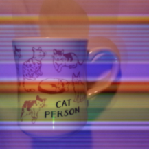
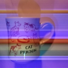
Figure 4: The simulation framework closely replicates the radiometric rolling shutter effect. The left image shows the simulation result and the right one is obtained in the physical experiments. Both of them are classified as “ping-pong ball.”

We characterize the attack algorithm’s performance across various camera configurations and environmental conditions. We find that the physical world results generally follow the trend of simulation results, implying that computing a successful simulation result will likely lead to a good physical success rate. fig:sim-phy confirms that the simulated image is visually similar to the physical one. To ensure the baseline imaging condition is valid, for all physical testing conditions, we capture images of the victim object under the same exposure, and similar ambient light and viewpoints. All of the baseline images are correctly classified as the object (e.g., coffee mug) with an average confidence of $68\%$.

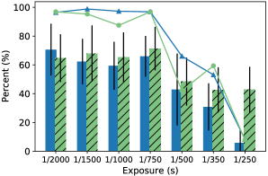
(a) Exposure

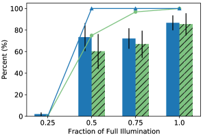
(b) Ambient light intensity

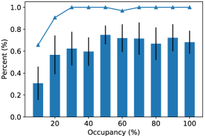
(c) Field of View (FoV)

Figure 5: Evaluating the attack success rate in simulation (Sim) and physical (Phys) for different settings (such as, ambient lighting and field-of-view) and camera parameters (such as, exposure).

Effect of Exposure.

We first explore the range of camera exposure values in which our attack would be effective. fig:conv-exposure shows the effect of various common exposure settings on the attack’s efficacy. We observe that the attack performs relatively well — approximately $94\%$ targeted attack success rate with $67\%$ confidence — at exposures $1/750$s and shorter. However, as exposures get longer the efficacy of the attack degrades and it stops working at exposures longer than $1/250$s. This confirms our hypothesis that longer exposures begin to approximate the global shutter effect. Based on the exposure results, we select a setting of $1/2000$s for the following experiments.

Ambient Lighting.

Attack performance depends on the lighting condition. We have experimentally observed that EoT under widely-varying lighting conditions does not converge for our attack. We emulate different ambient light conditions by controlling the LED output intensity as a fraction of total ambient lighting. We compute different signals for different ambient light condition and show their attack efficacy at an exposure of $1/2000$s in fig:ambient-light. As expected the attack performs better as relative strength of LEDs compared to the ambient light is higher.

Various Viewpoints.

We apply EoT to make our signal robust to viewpoint variations. In fig:viewpoint (row 1-2), we show the resulting images with our light signal for different camera orientations and distances for two different exposure values. All images are classified as “perfume”. Physical targeted attack success rate is $84\%$ with average confidence of $69\%$ at an exposure of $1/2000$s, and a success rate of $72\%$ with average confidence of $70\%$ at an exposure of $1/750$s. The averages are computed across $167$ and $194$ images at varying camera orientations. In  fig:viewpoint (row 3), we demonstrate the attack against a different object.

Field of View (FoV).

We optimize attack signals for different FoV occupancy values — the fraction of foreground object pixels to the whole image — and observe, in simulation, that the attack is stable until FoV occupancy $\leq 10\%$ (Fig. 5c). In the baseline case, the object is correctly classified at all FoV occupancy values, but the confidence reduces to 51% when FoV occupancy is $\leq 10\%$.

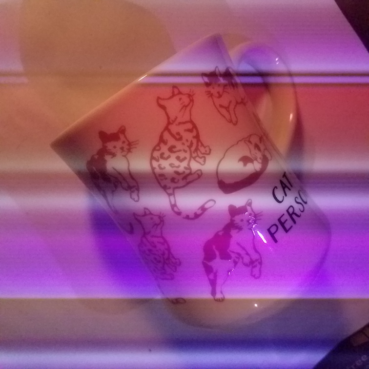
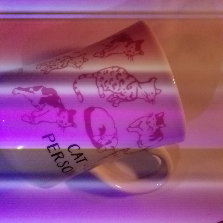
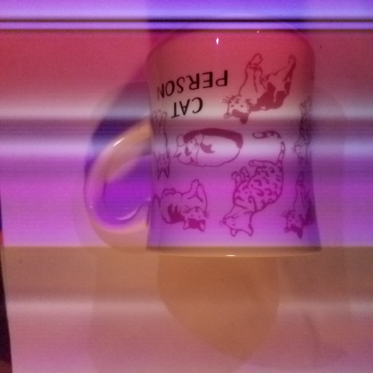
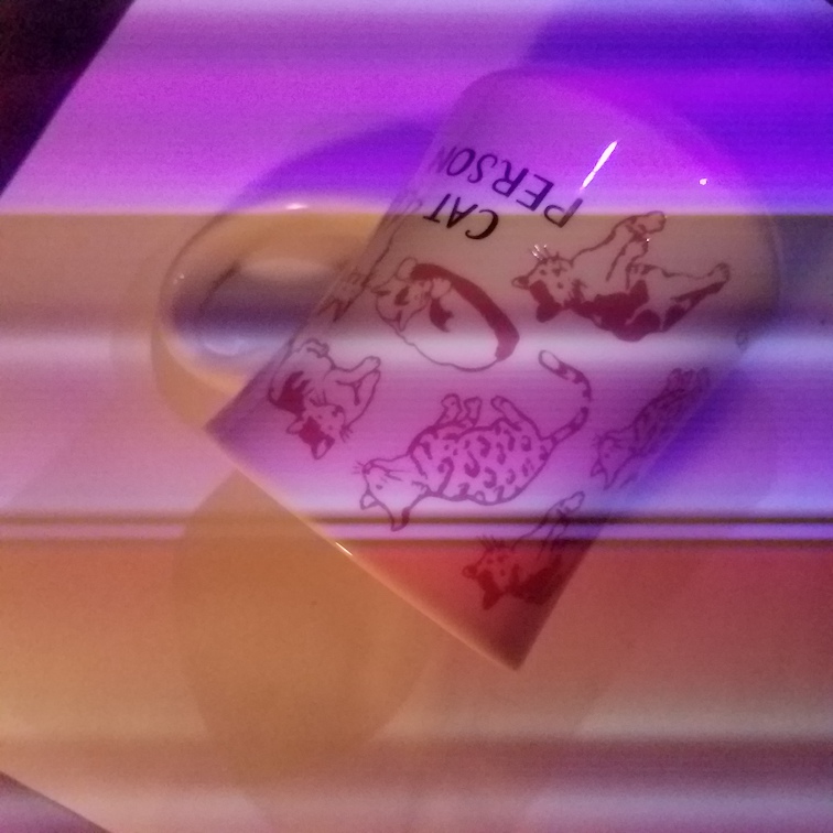
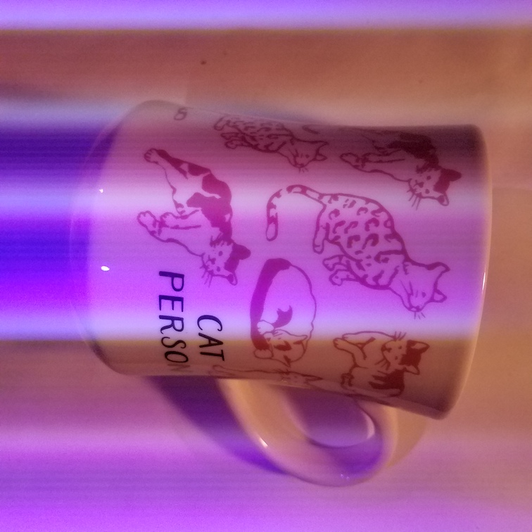
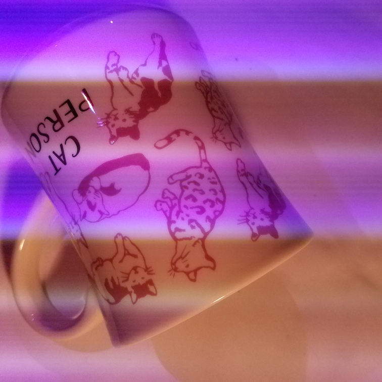
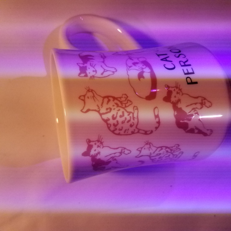
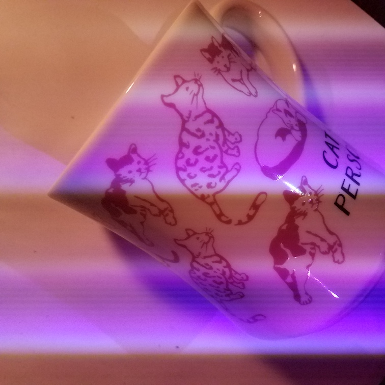
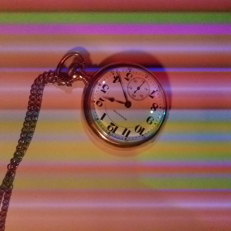
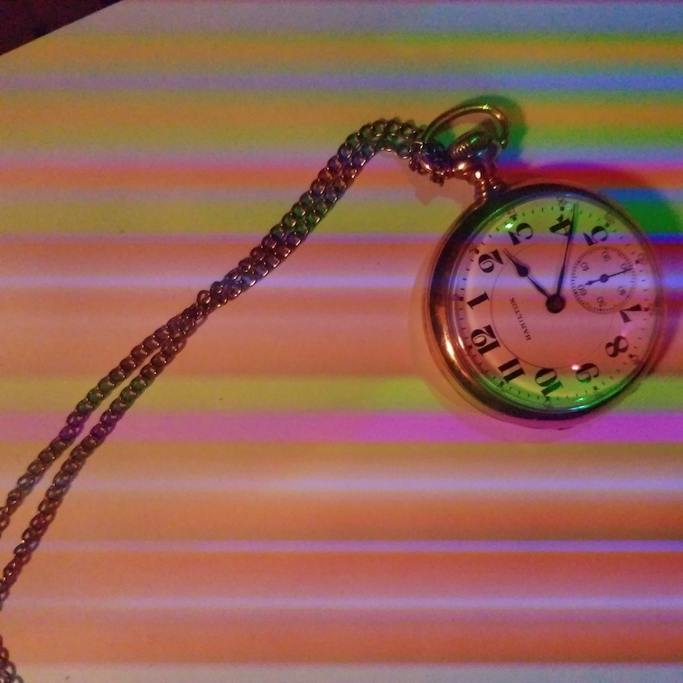
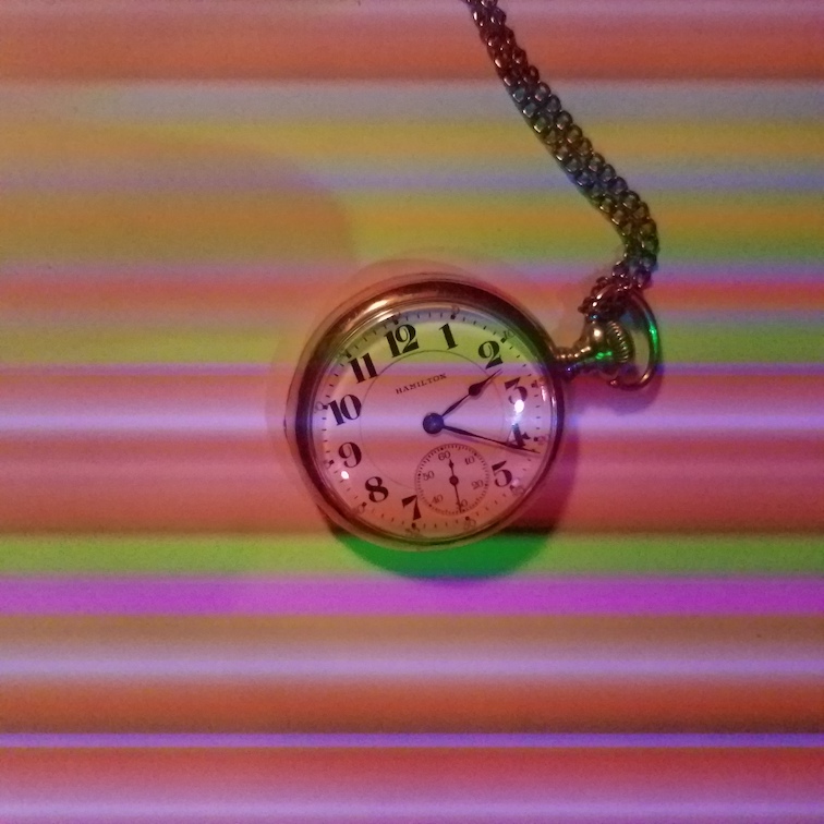
Figure 6: A sample of images taken at different camera orientations and two exposure values, $1/2000$s (first row) and $1/750$s (second row). Two different signals are used which are optimized for respective exposure values. The images are classified as “perfume” at an accuracy of $86\%$ (for exposure of $1/2000$s) and $72\%$ (for exposure of $1/750$s) with an average confidence of $69\%$. Third row - The images are classified as “whistle” at a targeted-attack success rate of $79\%$ with an average confidence of $66\%$.

7 Discussion and Conclusion

High frequency ambient sources.

For low exposure settings, ambient light sources powered by alternating current (AC) can induce their own flicker patterns [35]. This results in a sinusoidal flicker with a time period that depends on the frequency of the electric grid, which is generally 50Hz or 60Hz. We can address this in our imaging model by adding a signal image component to the ambient image, and use EoT to generate an attack that is invariant to this interference.

Deployment.

We envision the attack being deployed in low-light or controlled indoor lighting situations. For example, an attacker might compromise a LED bulb in a home to evade smart cameras or face recognition on a smart doorbell or laptop. Here, the attacker can acquire prior knowledge of the sensor parameters (e.g., they can purchase a similar device or lookup specs on the Internet). Given this knowledge, the attacker can pre-optimize a set of signals for commonly occurring imaging conditions for their use-case, measure the situation at deployment time and emit the appropriate signal.

Summary.

We create a novel way to generate physical adversarial examples that do not change the object, but manipulate the light that illuminates it. By modulating light at a frequency higher than human perceptibility, we show how to create an invisible perturbation that rolling shutter cameras will sense and the resulting image will be misclassified to the attacker-desired class.The attack is dynamic because an attacker can change the target class or gain robustness against specific ambient lighting or camera exposures by changing the modulation pattern on-the-fly. Our work contributes to the growing understanding of physical adversarial examples that exploit the differences in machine and human vision.

Acknowledgements. This work was supported in part by the University of Wisconsin-Madison Office of the Vice Chancellor for Research and Graduate Education with funding from the Wisconsin Alumni Research Foundation and NSF CAREER award 1943149.

Type	Transformation	Range
Physical	Rotation	$[0,360^{\circ}]$
	Horizontal Flip	{0, 1}
	Vertical Flip	{0, 1}
	Relative translation	$[0,0.7]$
	Relative Distance	$[1,1.5]$
	Relative lighting	$[0.8,1.2]$
Color Error (per channel)	Affine additive	$[-0.2,0.2]$
	Affine multiplicative	$[0.7,1.3]$

Table 2: Ranges for the transformation parameters used for generating and evaluating signals

Appendix A Distributions of Transformations

To make our adversarial signal effective in a physical setting, we use the EOT framework. We choose a distribution of transformations. The optimization produces an adversarial example that is robust under the distribution of transformations. Table 2 describes the transformations.

Physical transformations.

The relative translation involves moving the object in the image’s field of view. A translation value of 0 means the object is in the center of the image, while a value of 1 means the object is at the boundary of the image. The relative distance transform involves enlarging the object to emulate a closer distance. A distance value of 1 is the same as the original image, while for the value of 1.5, the object is enlarged to 1.5 times the original size.

Color correction.

Moreover, we apply a multiplicative brightening transformation to the ambient light image to account for small changes in ambient light. To account for the color correction, we used an affine transform of the form $Ax+B$, where $A$ and $B$ are real values sampled from a uniform distribution independently for each color channel.

Appendix B Additional Simulation Results

For evaluating the attack in a simulated setting, we select 5 classes from the ImageNet dataset. We select 7 target classes for each source class and report the results in Table 3. The attack generation and evaluation is the same as described previously. The attack success rate is calculated as the percentage of images classified as the target among 200 transformed images each averaged over all the possible signal offsets. tab:simulation-results-ball, 7 and 9 give a random sample of 4 transformed images for 3 source classes. For each source class, we give attacked images for 3 target classes.

Source (confid.)	Affinity targets	Attack success	Target confidence (StdDev)
Coffee mug (83%)	Perfume	99%	82% (13%)
	Petri dish	98%	88% (15%)
	Candle	98%	85% (18%)
	Menu	97%	84% (16%)
	Lotion	91%	75% (17%)
	Ping-pong ball	79%	68% (27%)
	Pill bottle	23%	40% (17%)
Street sign (87%)	Monitor	99%	94% (12%)
	Park bench	99%	90% (13%)
	Lipstick	84%	78% (20%)
	Slot machine	48%	59% (19%)
	Carousel	41%	61% (25%)
	Pool table	34%	47% (19%)
	Bubble	26%	37% (22%)
Teddy bear (93%)	Tennis ball	92%	88% (19%)
	Sock	76%	57% (22%)
	Acorn	75%	72% (25%)
	Pencil box	69%	48% (20%)
	Comic book	67%	44% (18%)
	Hour glass	64%	53% (25%)
	Wooden spoon	62%	53% (22%)
Soccer ball (97%)	Pinwheel	96%	87% (15%)
	Goblet	78%	55% (17%)
	Helmet	66%	59% (22%)
	Vase	44%	44% (17%)
	Table lamp	43%	46% (14%)
	Soap dispenser	37%	34% (16%)
	Thimble	10%	15% (02%)
Rifle (96%)	Bow	76%	64% (24%)
	Microphone	74%	63% (22%)
	Tripod	65%	65% (22%)
	Tool kit	57%	56% (22%)
	Dumbbell	35%	44% (21%)
	Binoculars	35%	40% (18%)
	Space bar	17%	33% (17%)

Table 3: Performance of affinity targeting using our adversarial light signals on five classes from ImageNet. For each source class we note the top 7 affinity targets, their attack success rate, and average classifier confidence of the target class. (Average is taken over all offsets values for 200 randomly sampled transformations.)

Original - Teddy Bear	Sock	Pencil box	Hour glass
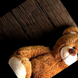
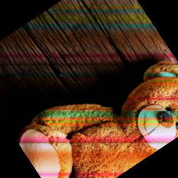
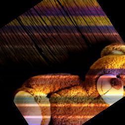
97%	90%	25%	20%
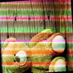
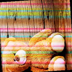
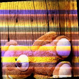
100%	83%	66%	61%
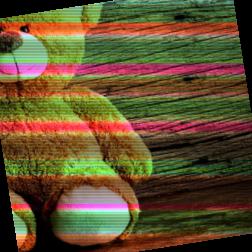
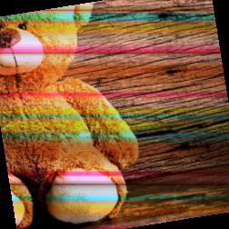
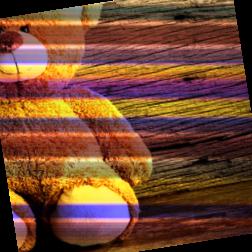
100%	91%	40%	83%
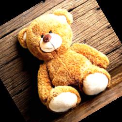
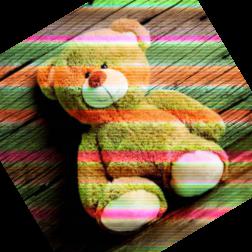
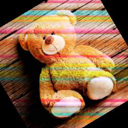
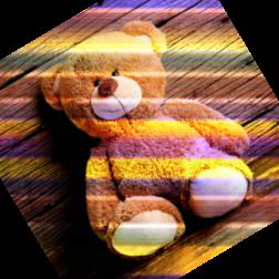
100%	78%	88%	86%

Figure 7: A random sample of targeted attacks against class - Teddy Bear. The attack is robust to viewpoint, distance and small lighting changes. The numbers denote the confidence values for the respective classes.

Original - Soccer ball	Pinwheel	Goblet	Helmet
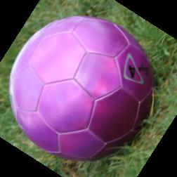
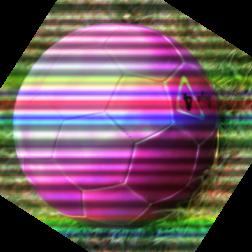
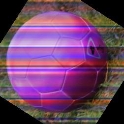
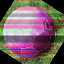
100%	96%	54%	70%
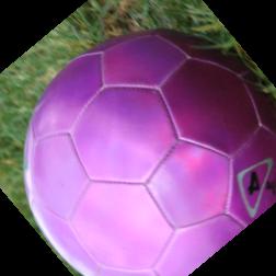
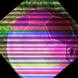
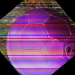
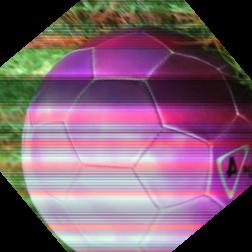
98%	98%	73%	58%
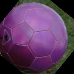
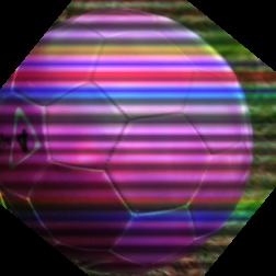
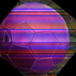
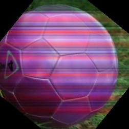
90%	83%	32%	40%
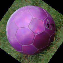
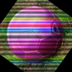
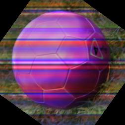
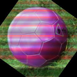
99%	88%	55%	24%

Figure 8: A random sample of targeted attacks against class - Soccer ball. The attack is robust to viewpoint, distance and small lightning changes. The numbers denote the confidence values for the respective classes.

Original - Rifle	Bow	Microphone	Tool kit
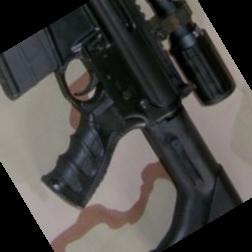
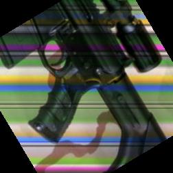
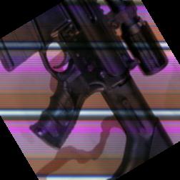
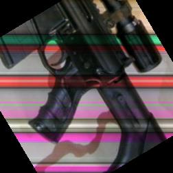
81%	94%	32%	70%
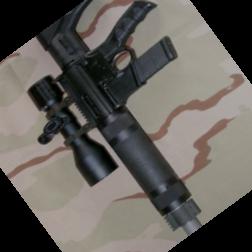
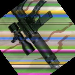
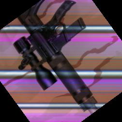
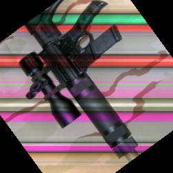
77%	100%	87%	50%
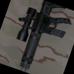
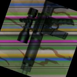
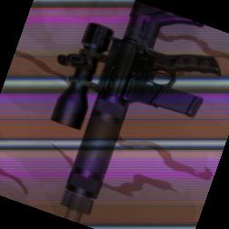
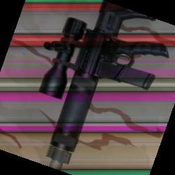
66%	98%	56%	72%
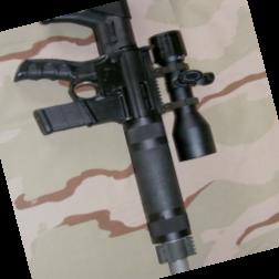
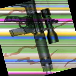
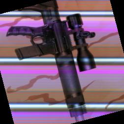
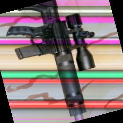
65%	100%	29%	77%

Figure 9: A random sample of targeted attacks against class - Rifle. The attack is robust to viewpoint, distance and small lightning changes. The numbers denote the confidence values for the respective classes.

References

- [1] Allied vision: ALVIUM 1800 u-1240. https://www.alliedvision.com/en/products/embedded-vision-cameras/detail/Alvium
- [2] AR023Z: CMOS image sensor, 2 mp, 1/2.7”. https://www.onsemi.com/products/sensors/image-sensors-processors/image-sensors/ar023z.
- [3] Cenek Albl, Zuzana Kukelova, Viktor Larsson, Tomas Pajdla, and Konrad Schindler. From two rolling shutters to one global shutter, 2020.
- [4] Matthew Anderson, Ricardo Motta, S. Chandrasekar, and Michael Stokes. Proposal for a standard default color space for the internet - srgb. In Color Imaging Conference, 1996.
- [5] Anish Athalye, Logan Engstrom, Andrew Ilyas, and Kevin Kwok. Synthesizing robust adversarial examples. volume 80 of Proceedings of Machine Learning Research, pages 284–293, Stockholmsmässan, Stockholm Sweden, 10–15 Jul 2018. PMLR.
- [6] Anish Athalye and Ilya Sutskever. Synthesizing robust adversarial examples. arXiv preprint arXiv:1707.07397, 2017.
- [7] Battista Biggio, Igino Corona, Davide Maiorca, Blaine Nelson, Nedim Šrndić, Pavel Laskov, Giorgio Giacinto, and Fabio Roli. Evasion attacks against machine learning at test time. In Joint European Conference on Machine Learning and Knowledge Discovery in Databases, pages 387–402. Springer, 2013.
- [8] Haitham Bou-Ammar, Holger Voos, and Wolfgang Ertel. Controller design for quadrotor uavs using reinforcement learning. In Control Applications (CCA), 2010 IEEE International Conference on, pages 2130–2135. IEEE, 2010.
- [9] Derek Bradley, Bradley Atcheson, Ivo Ihrke, and Wolfgang Heidrich. Synchronization and rolling shutter compensation for consumer video camera arrays. In IEEE Computer Society Conference on Computer Vision and Pattern Recognition Workshops, pages 1–8, Miami, FL, June 2009. IEEE.
- [10] Tom Brown, Dandelion Mane, Aurko Roy, Martin Abadi, and Justin Gilmer. Adversarial patch. 2017.
- [11] Nicholas Carlini and David Wagner. Towards evaluating the robustness of neural networks. In Security and Privacy (SP), 2017 IEEE Symposium on, pages 39–57. IEEE, 2017.
- [12] Chia-Kai Liang, Li-Wen Chang, and H.H. Chen. Analysis and Compensation of Rolling Shutter Effect. IEEE Transactions on Image Processing, 17(8):1323–1330, Aug. 2008.
- [13] Jia Deng, Wei Dong, Richard Socher, Li-Jia Li, Kai Li, and Li Fei-Fei. Imagenet: A large-scale hierarchical image database. In Computer Vision and Pattern Recognition, 2009. CVPR 2009. IEEE Conference on, pages 248–255. IEEE, 2009.
- [14] Kevin Eykholt, Ivan Evtimov, Earlence Fernandes, Bo Li, Amir Rahmati, Chaowei Xiao, Atul Prakash, Tadayoshi Kohno, and Dawn Song. Robust Physical-World Attacks on Deep Learning Visual Classification. In Computer Vision and Pattern Recognition (CVPR), June 2018.
- [15] Andreas Geiger, Philip Lenz, and Raquel Urtasun. Are we ready for autonomous driving? the kitti vision benchmark suite. In Computer Vision and Pattern Recognition (CVPR), 2012 IEEE Conference on, pages 3354–3361. IEEE, 2012.
- [16] Christopher Geyer, Marci Meingast, and Shankar Sastry. Geometric Models of Rolling-Shutter Cameras. In Proc. Omnidirectional Vision, Camera Networks and Non-Classical Cameras, pages 12–19, 2005.
- [17] Ian J Goodfellow, Jonathon Shlens, and Christian Szegedy. Explaining and harnessing adversarial examples. arXiv preprint arXiv:1412.6572, 2014.
- [18] Kensei Jo, Mohit Gupta, and Shree K. Nayar. Disco: Display-camera communication using rolling shutter sensors. 35(5), July 2016.
- [19] Namhoon Kim, Junsu Bae, Cheolhwan Kim, Soyeon Park, and Hong-Gyoo Sohn. Object distance estimation using a single image taken from a moving rolling shutter camera. Sensors, 20(14):3860, 2020.
- [20] Diederik Kingma and Jimmy Ba. Adam: A method for stochastic optimization. arXiv preprint arXiv:1412.6980, 2014.
- [21] Karl Koscher, Alexei Czeskis, Franziska Roesner, Shwetak Patel, Tadayoshi Kohno, Stephen Checkoway, Damon McCoy, Brian Kantor, Danny Anderson, Hovav Shacham, and Stefan Savage. Experimental security analysis of a modern automobile. In Proceedings of the 2010 IEEE Symposium on Security and Privacy, SP ’10, page 447–462, USA, 2010. IEEE Computer Society.
- [22] Alexey Kurakin, Ian Goodfellow, and Samy Bengio. Adversarial examples in the physical world. arXiv preprint arXiv:1607.02533, 2016.
- [23] Hui-Yu Lee, Hao-Min Lin, Yu-Lin Wei, Hsin-I Wu, Hsin-Mu Tsai, and Kate Ching-Ju Lin. Rollinglight: Enabling line-of-sight light-to-camera communications. In Proceedings of the 13th Annual International Conference on Mobile Systems, Applications, and Services, MobiSys ’15, page 167–180, New York, NY, USA, 2015. Association for Computing Machinery.
- [24] Juncheng Li, Frank Schmidt, and Zico Kolter. Adversarial camera stickers: A physical camera-based attack on deep learning systems. volume 97 of Proceedings of Machine Learning Research, pages 3896–3904, Long Beach, California, USA, 09–15 Jun 2019. PMLR.
- [25] Chia-Kai Liang, Li-Wen Chang, and Homer H Chen. Analysis and compensation of rolling shutter effect. IEEE Transactions on Image Processing, 17(8):1323–1330, 2008.
- [26] Timothy P Lillicrap, Jonathan J Hunt, Alexander Pritzel, Nicolas Heess, Tom Erez, Yuval Tassa, David Silver, and Daan Wierstra. Continuous control with deep reinforcement learning. arXiv preprint arXiv:1509.02971, 2015.
- [27] J. Linkemann and B. Weber. Global shutter, rolling shutter—functionality and characteristics of two exposure methods (shutter variants). White Paper, 2014.
- [28] Aleksander Madry, Aleksandar Makelov, Ludwig Schmidt, Dimitris Tsipras, and Adrian Vladu. Towards deep learning models resistant to adversarial attacks. arXiv preprint arXiv:1706.06083, 2017.
- [29] Seyed-Mohsen Moosavi-Dezfooli, Alhussein Fawzi, and Pascal Frossard. Deepfool: a simple and accurate method to fool deep neural networks. arXiv preprint arXiv:1511.04599, 2015.
- [30] Christian Mostegel, Markus Rumpler, Friedrich Fraundorfer, and Horst Bischof. Uav-based autonomous image acquisition with multi-view stereo quality assurance by confidence prediction. In Proceedings of the IEEE Conference on Computer Vision and Pattern Recognition Workshops, pages 1–10, 2016.
- [31] OpenPilot. OpenPilot on the Comma Two. https://github.com/commaai/openpilot, 2020.
- [32] TOMMY PALLADINO. Hololens 2, all the specs — these are the technical details driving microsoft’s next foray into augmented reality. https://hololens.reality.news/news/hololens-2-all-specs-these-are-technical-details-driving-microsofts-next-foray-into-augmented-reality-0194141/, 2019.
- [33] Nicolas Papernot, Patrick McDaniel, Somesh Jha, Matt Fredrikson, Z Berkay Celik, and Ananthram Swami. The limitations of deep learning in adversarial settings. In Security and Privacy (EuroS&P), 2016 IEEE European Symposium on, pages 372–387. IEEE, 2016.
- [34] Mahmood Sharif, Sruti Bhagavatula, Lujo Bauer, and Michael K Reiter. Accessorize to a crime: Real and stealthy attacks on state-of-the-art face recognition. In Proceedings of the 2016 ACM SIGSAC Conference on Computer and Communications Security, pages 1528–1540. ACM, 2016.
- [35] M. Sheinin, Y. Y. Schechner, and K. N. Kutulakos. Rolling shutter imaging on the electric grid. In 2018 IEEE International Conference on Computational Photography (ICCP), pages 1–12, 2018.
- [36] Christian Szegedy, Wojciech Zaremba, Ilya Sutskever, Joan Bruna, Dumitru Erhan, Ian Goodfellow, and Rob Fergus. Intriguing properties of neural networks. In International Conference on Learning Representations, 2014.
- [37] Kaidi Xu, Gaoyuan Zhang, Sijia Liu, Quanfu Fan, Mengshu Sun, Hongge Chen, Pin-Yu Chen, Yanzhi Wang, and Xue Lin. Adversarial t-shirt! evading person detectors in a physical world. In Andrea Vedaldi, Horst Bischof, Thomas Brox, and Jan-Michael Frahm, editors, Computer Vision – ECCV 2020, pages 665–681, Cham, 2020. Springer International Publishing.
- [38] Fangyi Zhang, Jürgen Leitner, Michael Milford, Ben Upcroft, and Peter Corke. Towards vision-based deep reinforcement learning for robotic motion control. arXiv preprint arXiv:1511.03791, 2015.
- [39] Shilin Zhu, Chi Zhang, and Xinyu Zhang. Automating visual privacy protection using a smart led. MobiCom ’17, page 329–342, New York, NY, USA, 2017. Association for Computing Machinery.