A Unified Mixture-View Framework for Unsupervised Representation Learning

Abstract

Recent unsupervised contrastive representation learning follows a Single Instance Multi-view (SIM) paradigm where positive pairs are usually constructed with intra-image data augmentation. In this paper, we propose an effective approach called Beyond Single Instance Multi-view (BSIM). Specifically, we impose more accurate instance discrimination capability by measuring the joint similarity between two randomly sampled instances and their mixture, namely spurious-positive pairs. We believe that learning joint similarity helps to improve the performance when encoded features are distributed more evenly in the latent space. We apply it as an orthogonal improvement for unsupervised contrastive representation learning, including current outstanding methods SimCLR [Chen et al.(2020a)Chen, Kornblith, Norouzi, and Hinton], MoCo [He et al.(2020)He, Fan, Wu, Xie, and Girshick], BYOL [Grill et al.(2020)Grill, Strub, Altché, Tallec, Richemond, Buchatskaya, Doersch, Pires, Guo, Azar, et al.] and SimSiam [Chen and He(2021)]. We evaluate our learned representations on many downstream benchmarks like linear classification on ImageNet-1k and PASCAL VOC 2007, object detection on MS COCO 2017 and VOC, etc. We obtain substantial gains with a large margin almost on all these tasks compared with prior arts.

1 Introduction

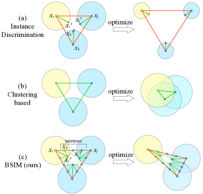
Figure 1: A schematic view of three self-supervised paradigms. Note $x_{i}$, $x_{j}$ and $x_{k}$ are different instances. Green lines link the positive pairs while red for negative. Circles show decision boundaries (same color for the same class). Instance discrimination narrows the boundary and pushes away all instances. Clustering-based methods might cluster wrong instances (e.g yellow and blue) due to a shortcut defect. BSIM mixes instances (where hue indicates the ratio) to construct spurious positive pairs (e.g ($x_{ij}$, $x_{i}^{\prime}$) and ($x_{ij}$, $x_{j}^{\prime}$). BSIM encourages contrastive competition among instances, thus being better at learning interclass and intraclass representation.

Unsupervised representational learning is now on the very rim to take over supervised representation learning. It is supposed to be a perfect solver for real-world scenarios full of unlabeled data. Among them, self-supervised learning has drawn the most attention for its good data efficiency and generalizability.

Self-supervised learning typically involves a proxy task to learn discriminative representations from self-derived labels. Among all manners of these proxy tasks [Noroozi and Favaro(2016), Gidaris et al.(2018)Gidaris, Singh, and Komodakis, Pathak et al.(2016)Pathak, Krahenbuhl, Donahue, Darrell, and Efros, Larsson et al.(2017)Larsson, Maire, and Shakhnarovich, Donahue et al.(2017)Donahue, Krähenbühl, and Darrell], instance discrimination [Wu et al.(2018)Wu, Xiong, Stella, and Lin, Liu et al.(2020)Liu, Zhang, Hou, Wang, Mian, Zhang, and Tang], known as contrastive representation learning, has emerged as the most effective paradigm. Its subsequent methods [Zhuang et al.(2019)Zhuang, Zhai, and Yamins, He et al.(2020)He, Fan, Wu, Xie, and Girshick, Chen et al.(2020a)Chen, Kornblith, Norouzi, and Hinton, Grill et al.(2020)Grill, Strub, Altché, Tallec, Richemond, Buchatskaya, Doersch, Pires, Guo, Azar, et al., Tian et al.(2020)Tian, Sun, Poole, Krishnan, Schmid, and Isola] have greatly reduced the gap between unsupervised and supervised learning. Specifically, instance discrimination features a Single Instance Multi-view (SIM) paradigm to separate different instances. It seeks to narrow the distance among multiple views of the same instance (e.g. an image), which are typically yielded from vanilla data augmentation policies like color jittering, cropping, resizing, applying Gaussian noise. Consequently, the invariance of the network is easily bounded by these limited augmentations. Since different instances are continuously driven apart, SIM prevents itself from characterizing the relations among different instances from the same class, as opposed to supervised classification.

Meanwhile, clustering-based self-supervised methods [Caron et al.(2018)Caron, Bojanowski, Joulin, and Douze, Zhan et al.(2020a)Zhan, Xie, Liu, Ong, and Loy] alternate feature clustering with learning to capture similarities among different instances. These methods avoid the intrinsic weakness of instance discrimination, but suffer from a so-called ‘shortcut’ problem, i.e., when two instances are occasionally grouped into a cluster, their similarity will be further enhanced. As a result, the training easily drifts into trivial solutions, e.g, merely grouping images in similar color or texture.

In view that instance discrimination pushes apart different instances indistinguishably as shown in Fig. 1(a), and clustering-based methods are easily trapped in shortcut issues as shown in Fig. 1(b), we are motivated to explore a new paradigm to distinguish both intraclass and interclass instances. In this work, we propose BSIM to learn better representations that capture high-level inter-image relations, which also potentially avoid the above-mentioned shortcut issue. To make the minimal modification from previous works, BSIM shares similar pipelines to SimCLR [Chen et al.(2020a)Chen, Kornblith, Norouzi, and Hinton], MoCo [He et al.(2020)He, Fan, Wu, Xie, and Girshick], BYOL [Grill et al.(2020)Grill, Strub, Altché, Tallec, Richemond, Buchatskaya, Doersch, Pires, Guo, Azar, et al.] and SimSiam [Chen and He(2021)], while focusing on a new way to construct positive pairs.

Specifically, as shown in Fig. 1(c), BSIM first creates mixtures using CutMix [Yun et al.(2019)Yun, Han, Oh, Chun, Choe, and Yoo] among instances by proportion, e.g, $x_{ij}$ that mixes $\lambda$ of $x_{i}$ and $(1-\lambda)$ of $x_{j}$, where $\lambda\in(0,1)$ obeys a Beta distribution. Different from instance discrimination that constructs positive pairs between two views from the same image, BSIM makes use of mixed views $x_{ij}$ to create what we call spurious-positive pairs $\left(x_{ij},x_{i}^{\prime}\right)$ and $\left(x_{ij},x_{j}^{\prime}\right)$. The optimization also proportionally takes $\lambda$ into account for computing the losses. The interaction of spurious-positive pairs compete for an equilibrium state when grouping intra-instance and inter-instance views, modulated by the distribution of $\lambda$. Meantime, negative pairs keep pushing away different instances. As a result, BSIM encourages contrastive competition among instances, leaning towards exploring higher-level inter-image relations. Since BSIM does not maintain dynamically changing pseudo labels as clustering-based methods, the shortcut issue is naturally avoided. The contribution of this paper is twofold,

• We propose a novel paradigm, namely BSIM, to encourage contrastive competition among instances for higher-level representation learning. Specifically, we generate spurious positive examples using CutMix mixture, and we quantitatively score the distance between any image pairs by formulating a new contrastive loss .

• BSIM is a general-purpose enhancement to existing methods that rely on instance discrimination (e.g. SimCLR, MoCo, BYOL, SimSiam). BSIM boosts performance for prior arts by clear margins and the gain from BSIM (e.g. BYOL-BSIM) is even comparable to the latest elaborately designed methods such as SimSiam [Chen and He(2021)]. Moreover, it requires minimal modification to current self-supervised learning frameworks while adding neglectable cost. In general, BSIM-powered networks achieve state-of-the-art performance in a large body of standard benchmarks.

2 Related Work

Self-supervised learning based on contrastive loss. Early methods focus on devising proxy tasks to either reconstruct the image after transformations [Larsson et al.(2017)Larsson, Maire, and Shakhnarovich, Pathak et al.(2016)Pathak, Krahenbuhl, Donahue, Darrell, and Efros, Zhang et al.(2017)Zhang, Isola, and Efros], or predict the configurations of applied transformation on a single image [Doersch et al.(2015)Doersch, Gupta, and Efros, Dosovitskiy et al.(2014)Dosovitskiy, Springenberg, Riedmiller, and Brox, Noroozi and Favaro(2016), Gidaris et al.(2018)Gidaris, Singh, and Komodakis]. Till recently contrastive loss based approaches [He et al.(2020)He, Fan, Wu, Xie, and Girshick, Chen et al.(2020a)Chen, Kornblith, Norouzi, and Hinton, Grill et al.(2020)Grill, Strub, Altché, Tallec, Richemond, Buchatskaya, Doersch, Pires, Guo, Azar, et al., Caron et al.(2020a)Caron, Misra, Mairal, Goyal, Bojanowski, and Joulin] emerge as the mainstream paradigm, which features two components: the selection of positive or negative examples and the contrastive loss design. This routine leverages different augmented views of an image to construct positive pairs, while deeming other images as negative samples.

Particularly, SimCLR [Chen et al.(2020a)Chen, Kornblith, Norouzi, and Hinton] produces positive and negative pairs within a mini-batch of training data and chooses InfoNCE [Oord et al.(2018)Oord, Li, and Vinyals] loss to train the feature extraction backbone. It requires a large batch-size to effectively balance the positive and negative ones. MoCo [He et al.(2020)He, Fan, Wu, Xie, and Girshick] makes use of a feature queue to store negative samples, which greatly reduces high memory cost in [Chen et al.(2020a)Chen, Kornblith, Norouzi, and Hinton]. Moreover, it proposes a momentum network to boost the consistency of features. BYOL [Grill et al.(2020)Grill, Strub, Altché, Tallec, Richemond, Buchatskaya, Doersch, Pires, Guo, Azar, et al.] challenges the indispensability of negative examples and achieves impressive performance by only using positive ones. A mean square error loss is applied to make sure that positive pairs can predict each other. SimSiam [Chen and He(2021)] utilizes stop-gradient as an alternative method to avoid mode collapse, simplifying the design compared to prior arts.

Besides, carefully designed augmentations to build positive pairs are proven to be critical for good performance [Chen et al.(2020a)Chen, Kornblith, Norouzi, and Hinton, Tian et al.(2020)Tian, Sun, Poole, Krishnan, Schmid, and Isola, Chen et al.(2020b)Chen, Fan, Girshick, and He, Misra and Maaten(2020), Tian et al.(2019)Tian, Krishnan, and Isola, Asano et al.(2019)Asano, Rupprecht, and Vedaldi, Gontijo-Lopes et al.(2020)Gontijo-Lopes, Smullin, Cubuk, and Dyer, Wang and Isola(2020)], because appropriate augmentations modulate the distribution of positive examples in the feature space. SwAV [Caron et al.(2020a)Caron, Misra, Mairal, Goyal, Bojanowski, and Joulin] obtains the state-of-the-art unsupervised performance by using a mixture of views in different resolutions in place of two full-resolution ones. In the meantime, some researches study the role of hard negative examples [Iscen et al.(2018)Iscen, Tolias, Avrithis, and Chum, Kalantidis et al.(2020)Kalantidis, Sariyildiz, Pion, Weinzaepfel, and Larlus, Chuang et al.(2020)Chuang, Robinson, Yen-Chen, Torralba, and Jegelka, Xie et al.(2020)Xie, Zhan, Liu, Ong, and Loy, Wu et al.(2020)Wu, Zhuang, Mosse, Yamins, and Goodman]. However, all the above approaches try to push each image instance away from each other by regarding them as its negative samples. Is it possible to model the vicinity relation by measuring that distance quantitatively? To our best knowledge, this problem is rarely studied in the field of self-supervised learning and BSIM is aimed to bridge this gap.

Mixture as a regularization technique in supervised learning. Mixture of training samples like Mixup [Zhang et al.(2018)Zhang, Cisse, Dauphin, and Lopez-Paz], CutMix [Yun et al.(2019)Yun, Han, Oh, Chun, Choe, and Yoo], and Manifold Mixup [Verma et al.(2019)Verma, Lamb, Beckham, Najafi, Mitliagkas, Lopez-Paz, and Bengio] has been proved to be a strong regularization for supervised learning, based on the principle of vicinal risk minimization [Chapelle et al.(2001)Chapelle, Weston, Bottou, and Vapnik]. It is designed to model vicinity relation across different classes other than vanilla data augmentation tricks that only considers the same class. CutMix [Yun et al.(2019)Yun, Han, Oh, Chun, Choe, and Yoo] debates that Mixup introduces unnatural artifacts by mixing the whole image region while Cutout [DeVries and Taylor(2017)] might pay attention to less discriminative parts. CutMix claims to effectively localize the two classes instead. [Tokozume et al.(2018a)Tokozume, Ushiku, and Harada] argues that mixing images is akin to mixing sounds [Tokozume et al.(2018b)Tokozume, Ushiku, and Harada] for CNNs, although not easily perceptible for humans. Other than deeming it as vanilla data augmentation that adds data variation, they consider it as an enlargement of Fisher’s criterion [Fisher(1936)], i.e., the ratio of the between-class scatter to the within-class scatter, and it regularizes positional relationship among latent feature distributions. Furthermore, [Thulasidasan et al.(2019)Thulasidasan, Chennupati, Bilmes, Bhattacharya, and Michalak] notices that label smoothing during mixup training has a calibration effect which regularizes over-confident predictions.

3 Methodology

Different from the wide use of augmentation as a useful regularization in supervised learning, how to use it in unsupervised learning remains to be an open problem. Using the mixture solely as one of data augmentation techniques to produce positive pairs significantly weakens the performance of MoCoV2 [Chen et al.(2020b)Chen, Fan, Girshick, and He] (Table 1). This preferred regularization in supervised learning seems inherently incompatible with contrastive learning: drawing near multiple augmented views of an image while pushing away from the others, which we call Single Instance Multi-view (SIM) for simplicity. Instead, a mixture view shall be drawn close to both source images. This motivates us to scheme an alternative strategy for contrastive learning. There are two basic and coupled problems to be answered: how to address the degradation and how to design feasible mixtures.

Method	Epoch	SVM @VOC2007	LC @ImageNet
MoCoV2 (He et al.(2020)He, Fan, Wu, Xie, and Girshick)	200	83.81%	67.5%
MoCoV2+MixAug	200	80.10% (-3.71%$\downarrow$)	64.6% (-2.9%$\downarrow$)

Table 1: Regarding mixture as an extra data augmentation (MoCoV2+MixAug) weakens its performance severely. LC: linear classification on ImageNet.

The central principle of contrastive learning is to encode semantically similar views (positive pairs) into latent representations that are close to each other while driving dissimilar ones (negative pairs) apart. A major question is how to effectively synthesize positive and negative pairs given a dataset of i.i.d. samples as raised by [Tian et al.(2020)Tian, Sun, Poole, Krishnan, Schmid, and Isola]. Another question engages the design of contrastive loss. Next, we discuss BSIM in details to address both.

3.1 Spurious-Positive Views From Multiple Images

Given a set of images $\mathcal{D}$, two images $x_{1},x_{2}$ sampled uniformly from $\mathcal{D}$, and two image augmentation distributions of $\mathcal{T}^{\prime}$ and $\mathcal{T}^{\prime\prime}$ (whether $\mathcal{T}^{\prime}$ and $\mathcal{T}^{\prime\prime}$ are the same depends on different methods), we first generate a new example $x_{1,2}^{\prime}$ by mixing $t^{\prime}(x_{1})$ and $t^{\prime}(x_{2})$, where $t^{\prime}\sim\mathcal{T}^{\prime}$. Specifically, $x_{1,2}^{\prime}$ borrows $\lambda$ region from $t^{\prime}(x_{1})$ and remaining ($1-\lambda$) part from $t^{\prime}(x_{2})$. Thus, $x_{1,2}^{\prime}$ has two spurious-positive examples, i.e., $t^{\prime\prime}(x_{1})$ and $t^{\prime\prime}(x_{2})$ , where $t^{\prime\prime}\sim\mathcal{T}^{\prime\prime}$. These images are encoded by a neural network $f$ to extract high-level features, followed by a projection head $g$ that maps the representation to a space ready to apply contrastive loss. The projection function is often implemented as a simple MLP network. For a better understanding, we give a schematic construction under SimCLR framework in Fig. 8 (supp.).

The distance between the newly mixed example and its parents is controlled by $\lambda$. BSIM uses a popular and handy option to generation $\lambda$ from Beta distributions, i.e., $\lambda\sim\beta$($\alpha$, $\alpha$), where $\alpha$ is a hyper-parameter. It is evident that it would degrade to the single-instance multi-view case if $\lambda$ is always 0 or 1 when $\alpha\rightarrow 0$. That being said, BSIM is a generalization of SIM so that previous SIM methods reside within our larger framework.

3.2 Loss Functions of BSIM

It’s intuitive to change loss functions since spurious-positive examples are introduced. For example, it’s unreasonable to assign a new instance generated by half mixing two images (a dog and a cat, $\lambda=0.5$) to a dog or cat. Human would easily tell this image is half cat and half dog. This means its projected feature in the high-dimensional latent space should be nearby a dog, as well as a cat, but much far from an orangutan. This motivates us to design a particular loss for BSIM on top of the spurious-positive views, shown in Fig. 2. Specifically, we adapt our method to four popular frameworks SimCLR [Chen et al.(2020a)Chen, Kornblith, Norouzi, and Hinton], MoCo [He et al.(2020)He, Fan, Wu, Xie, and Girshick], BYOL [Grill et al.(2020)Grill, Strub, Altché, Tallec, Richemond, Buchatskaya, Doersch, Pires, Guo, Azar, et al.] and SimSiam [Chen and He(2021)]. In order to make our paper more readable, we roughly follow the same naming conventions as these papers and list the symbol notations in Table 8 (supp.).

Figure 2: Our generic BSIM framework (b) serves as a plug-and-play adds-on for current contrastive learning paradigm (a). Note $\mathcal{T}$ and $\mathcal{T}^{\prime}$ are augmentation policy distributions.

SimCLR-BSIM.

SimCLR uses a single augmentation distribution, i.e. $\mathcal{T}^{\prime}$ and $\mathcal{T}^{\prime\prime}$ are identical herein. The encoder network $f$ encodes $x_{1,2}^{\prime}$ as $f(x_{1,2}^{\prime})$. Note $x_{1,2}^{\prime}$ should show similarities with $x_{1}^{\prime\prime}$ as well as $x_{2}^{\prime\prime}$, which is measured by the $\mathrm{sim}$ function in the projected $z$ space. We follow the definition in [Chen et al.(2020a)Chen, Kornblith, Norouzi, and Hinton] for the similarity function as $\mathrm{sim}(\bm{z}_{i},\bm{z}_{j})=\bm{z}_{i}^{\top}\bm{z}_{j}/(\lVert\bm{z}_{i}\rVert\lVert\bm{z}_{j}\rVert)$. We use $\lambda$ to regularize these similarities and the matching loss can be formulated as,

$$\begin{split}\ell^{\prime}_{i}(\lambda)\!=\!-\lambda&\log\frac{e^{\mathrm{sim}(\bm{z}_{i,j}^{\prime},\bm{z}_{i}^{\prime\prime})/\tau}}{\sum_{k=1}^{N}[e^{\mathrm{sim}(\bm{z}_{i,j}^{\prime},\bm{z}_{k}^{\prime\prime})/\tau}\!+\!\mathbbm{1}\cdot e^{\mathrm{sim}(\bm{z}_{i,j}^{\prime},\bm{z}_{i,k}^{\prime})/\tau}]}\\ \!-\!(1\!-\!\lambda)&\log\frac{e^{\mathrm{sim}(\bm{z}_{i,j}^{\prime},\bm{z}_{j}^{\prime\prime})/\tau}}{\sum_{k=1}^{N}[e^{\mathrm{sim}(\bm{z}_{i,j}^{\prime},\bm{z}_{k}^{\prime\prime})/\tau}\!+\!\mathbbm{1}\cdot e^{\mathrm{sim}(\bm{z}_{i,j}^{\prime},\bm{z}_{i,k}^{\prime})/\tau}]}.\\ \text{where\quad}\mathbbm{1}&=\begin{cases}1&k\not\in\{i,j\}\\ 0&\text{otherwise}\end{cases}\end{split}$$ (1)

Similarly, we can formulate $\ell_{i}^{\prime\prime}$ if we use $x_{1,2}^{\prime\prime}$ as the anchor. Hence, the NT-Xent [Chen et al.(2020a)Chen, Kornblith, Norouzi, and Hinton] loss is defined by the summation of each individual loss within the mini-batch data of size $N$ as,

$$L_{\texttt{NT-Xent}}(\lambda)=\frac{1}{2N}\sum_{k=1}^{N}\ell_{i}^{\prime}(\lambda)+\ell_{i}^{\prime\prime}(\lambda),\hskip 5.0pt\lambda\sim\beta(\alpha,\alpha).$$ (2)

SimCLR [Chen et al.(2020a)Chen, Kornblith, Norouzi, and Hinton] has $2N$ positive pairs and $2N(N-1)$ negative ones in total at each iteration. Whereas, our method includes $4N$ spurious-positive pairs, i.e., $(x_{i,j}^{\prime},x_{i}^{\prime\prime})$, $(x_{i,j}^{\prime},x_{j}^{\prime\prime})$, $(x_{i,j}^{\prime\prime},x_{i}^{\prime})$, $(x_{i,j}^{\prime\prime},x_{j}^{\prime})$, and $2N(N-2)$ negative ones. The proposed method is depicted in Figure 8 (supp.).

MoCo-BSIM.

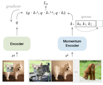
Figure 9: Applying BSIM to MoCo. Given a batch of images, we mix them in a pair-wise manner to produce $x_{q}$ (only one mixture is shown for simplicity). We encode the mixed images as query $q$ and the whole current batch as keys $k$. We thus generate spurious-positive pairs from $q$ and $k$, and the current queue is used as negative samples.

We produce the query $q$ of MoCo by forwarding the mixed image controlled by $\lambda$. We illustrate the procedure in Fig. 9 (supp.).

$$\small\mathcal{L}_{q}=-\lambda\log\frac{\exp(q\cdot k^{\lambda}_{+}/\tau)}{\sum_{i=1}^{N}\exp(q\cdot k_{i}/\tau)}-(1-\lambda)\log\frac{\exp(q\cdot k^{1-\lambda}_{+}/\tau)}{\sum_{i=1}^{N}\exp(q\cdot k_{i}/\tau)}$$ (3)

where $k^{\lambda}_{+}$ and $k^{1-\lambda}_{+}$ represent the corresponding key of images that produced the mixture respectively, and $k_{i}$ are the keys in the current queue. $\tau$ is the softmax temperature.

BYOL-BSIM.

BYOL-BSIM generates two augmented views $x_{1}^{\prime}\triangleq t^{\prime}(x_{1})$ and $x_{1}^{\prime\prime}\triangleq t^{\prime\prime}(x_{1})$ from $x_{1}$ by applying respectively image augmentations $t^{\prime}\sim\mathcal{T}^{\prime}$ and $t^{\prime\prime}\sim\mathcal{T}^{\prime\prime}$. Following the same procedure, we produce $x_{2}^{\prime}$ and $x_{2}^{\prime\prime}$. Then we produce a new image $x^{\prime}_{1,2}$ by $\lambda$-based mixture $x_{1}^{\prime}$ and $x_{2}^{\prime}$ through cutmix. The online network outputs $y^{\prime}_{\theta}\triangleq f_{\theta}(x^{\prime}_{1,2})$ and the projection $z^{\prime}_{\theta}\triangleq g_{\theta}(y^{\prime})$. The target network yields two $\ell_{2}$-normalized projections $\bar{z}^{\prime\prime}_{1}$, $\bar{z}^{\prime\prime}_{2}$ from $x^{\prime\prime}_{1}$ and $x^{\prime\prime}_{2}$.

We sum up the MSE loss between the projection of the mixed image and its parents by the mixture coefficient $\lambda$. This process is shown in Fig. 10 (supp.). Formally, the loss is:

$$\small\begin{split}\mathcal{L}^{\prime}_{{\theta},\xi}=-2[\lambda\frac{\langle q^{\prime}_{\theta}(z^{\prime}_{\theta}),z^{\prime\prime}_{i,\xi}\rangle}{\big{\|}q^{\prime}_{\theta}(z^{\prime}_{\theta})\big{\|}_{2}\cdot\big{\|}z^{\prime\prime}_{i,\xi}\big{\|}_{2}}+(1-\lambda)\frac{\langle q^{\prime}_{\theta}(z^{\prime}_{\theta}),z^{\prime\prime}_{j,\xi}\rangle}{\big{\|}q^{\prime}_{\theta}(z^{\prime}_{\theta})\big{\|}_{2}\cdot\big{\|}z^{\prime\prime}_{j,\xi}\big{\|}_{2}}]\end{split}$$ (4)

Note $z^{\prime\prime}_{i,\xi}$ and $z^{\prime\prime}_{j,\xi}$ mean the projection of the representation of $x_{i}^{\prime\prime}$ and $x_{j}^{\prime\prime}$ generated by the target network. We obtain $\mathcal{L}^{\prime\prime}_{{\theta},\xi}$ by using $x_{1}^{\prime\prime}$ and $x_{2}^{\prime\prime}$ as the input of online network. Note that BYOL doesn’t rely on negative samples. The normalized projection is on the sphere of a unit ball in the high dimensional space, see Fig. 7 (supp.).

SimSiam-BSIM.

Since SimSiam utilizes the same loss as BYOL, we use exactly the same loss form as Eq 4 with scale 0.5 to match the loss in SimSiam [Chen and He(2021)].

WBSIM.

Alternatively, we offer BSIM as a general adds-on by adding a weighted BSIM (WBSIM) loss to the usual SIM losses, see Sec B (supp.) for details.

3.3 Mixture Strategy Design

CutMix and Mixup [Zhang et al.(2018)Zhang, Cisse, Dauphin, and Lopez-Paz] are two popular strategies of generating mixtures at image level. Whereas we don’t utilize Mixup because it is less natural, even humans cannot easily tell the mixture coefficient $\lambda$ simply by checking the mixed image. We compare Mixup with CutMix via carefully controlled experiments (both with BSIM loss and the same hyper-parameter settings) under the framework of MoCoV2. Results from Table 2 disapprove of the use of Mixup in producing spurious-positive examples. The observation differs from supervised learning, where both boost the performance.

Method	SVM	SVM Low-Shot (96)
MoCoV2 [He et al.(2020)He, Fan, Wu, Xie, and Girshick]	83.81%	82.01$\pm$0.13%
MoCoV2 (w/ Mixup, $\alpha$=1.0)	82.50%	80.54$\pm$0.26%
MoCoV2 (w/ Mixup, $\alpha$=0.5)	82.80%	80.58$\pm$0.31%
MoCoV2-BSIM (w/ CutMix, $\alpha$=1.0)	84.55%	82.65$\pm$0.34%

Table 2: SVM evaluations on PASCAL VOC2007. Mixup deteriorates the performance of the baseline.

We also compare their performance using VOC object detection under the same metrics in Sec C.3 (supp.). The result is shown in Table 3. Mixup fails to improve the performance of its baseline without mixtures. In contrast, CutMix can improve the detection performance. Therefore, we utilize CutMix as our default mixture strategy.

Method	AP50	AP75	AP
No Mix	82.4%	63.6%	57.0%
Mixup ($\alpha$=1.0)	82.2%(-0.2$\downarrow$)	63.4%(-0.2$\downarrow$)	56.9%(-0.1$\downarrow$)
CutMix ($\alpha$=1.0)	82.7%(+0.3$\uparrow$)	64.0%(+0.4$\uparrow$)	57.3%(+0.3$\uparrow$)

Table 3: Object detection results under the MoCoV2 framework on PASCAL VOC trainval07+12.

4 Experiments

Setup.

We generally follow the compared methods. Details and cost are in Sec C (supp.). Object detection and instance segmentation experiments are given in Sec C.3 (supp.).

4.1 Evaluation on Linear Classification

Linear SVM classification on VOC2007.

The results are shown in Table 4. In most cases, BSIM consistently boosts the baselines by about $1\%$ mAP. Particularly, BYOL-BSIM is boosted by a clear margin: 1.4% mAP. BYOL-BSIM300 outperforms the supervised pre-trained baseline with 0.4% higher mAP. BYOL-BSIM (200 epochs’ training) is comparable to BYOL300 (300 epochs). Noticeably, WBSIM further boosts the performance. MoCoV2 benefits 1% mAP from BSIM, and an extra 0.6% higher mAP from WBSIM, indicating that BSIM is complementary to SIM.

Method		SVM	SVM Low-Shot (%mAP)
		%mAP	1	2	4	8	16	32	64	96
Supervised		87.2	53.0	63.6	73.7	78.8	81.8	83.8	85.2	86.0
SimCLR (chen2020simple)		79.0	32.5	40.8	50.4	59.1	65.5	70.1	73.6	75.4
SimCLR-BSIM		80.0	33.9	44.7	50.9	60.5	67.8	72.0	75.4	77.2
MoCo (he2020momentum)		79.2	30.0	37.7	47.6	58.8	66.0	70.6	74.6	76.1
MoCoV2 (chen2020improved)		83.8	43.7	55.2	63.2	71.5	75.4	79.1	81.2	82.0
MoCoV2-BSIM		84.8	50.0	53.9	65.3	72.4	76.3	79.3	81.7	82.8
MoCoV2-WBSIM		85.4	46.5	56.9	64.6	74.7	78.2	80.6	82.8	83.7
BYOL (grill2020bootstrap)		85.1	44.5	52.1	62.9	70.9	76.2	79.5	81.9	83.1
BYOL-BSIM		86.5	42.6	55.9	64.6	72.7	78.8	81.9	83.6	84.6
BYOL300 (grill2020bootstrap)		86.6	42.5	56.1	64.7	73.0	77.7	82.2	83.7	84.7
BYOL-BSIM300		87.6	45.7	54.5	66.4	75.0	79.8	83.2	85.2	86.0
BYOL-WBSIM300		87.7	44.1	60.7	68.1	76.0	81.0	83.6	85.2	86.3
SwAV (caron2020unsupervised)⋆		85.4	-	-	-	-	-	-	-	-

Table 4: ResNet-50 linear SVMs mAP on VOC07 [Everingham et al.(2010)Everingham, Van Gool, Williams, Winn, and Zisserman] classification using two 224$\times$ 224 views. BYOL variants with “300” are trained for 300 epochs as [Grill et al.(2020)Grill, Strub, Altché, Tallec, Richemond, Buchatskaya, Doersch, Pires, Guo, Azar, et al.]. ^⋆: SwAV is trained for 400 epochs.

Low-shot classification on VOC2007.

The results are shown in Table 4. BSIM helps all baselines to achieve better performance by substantial margins. It’s interesting to see that BYOL-BSIM300 gradually bridge its gap from the supervised baseline. When the number of the training set is more than 64, it’s comparable to the supervised version.

Linear classification on ImageNet.

The results are shown in Table 5, where the performance of the competing methods are extracted from [Zhan et al.(2020b)Zhan, Xie, and Xie].

Method	Epoch	Backbone		Top-1 Accuracy
InfoMin Aug (tian2020makes)	200	R50		70.1
MoCo (he2020momentum)	200	R50		61.0
SimCLR(chen2020simple)	200	R50		61.6
SimCLR-BSIM	200	R50		62.3 (+0.7$\uparrow$)
MoCoV2 (chen2020improved)	200	R50		67.5
MoCoV2-BSIM	200	R50		68.0 (+0.5$\uparrow$)
MoCoV2-WBSIM	200	R50		68.4 (+0.9$\uparrow$)
BYOL (grill2020bootstrap)	200	R50		69.1
BYOL-BSIM	200	R50		69.8 (+0.7$\uparrow$)
BYOL (grill2020bootstrap)†	300	R50		72.3
BYOL-BSIM	300	R50		72.7 (+0.4$\uparrow$)
BYOL-WBSIM	300	R50		73.0 (+0.7$\uparrow$)
SimSiam (chen2020exploring)	200	R50		70.0
SimSiam-BSIM (chen2020exploring)	200	R50		70.4(+0.4$\uparrow$)
SimSiam-WBSIM (chen2020exploring)	200	R50		70.8(+0.8$\uparrow$)
SwAV (caron2020unsupervised)	200	R50		69.1
SwAV (caron2020unsupervised)	400	R50		70.7

Table 5: Linear classification on ImageNet (top-1 center-crop accuracy on the validation set). All models are trained with two 224$\times$224 views. ^†: reproduced. SwAV result is from SimSiam [Chen and He(2021)].

4.2 Evaluation on Semi-supervised Classification

Results are shown in Table 6. BSIM improves the baselines by significant margins, especially when the amount of available labels is small. MoCoV2-BSIM obtains $44.3\%$ top-1 accuracy, which is $5.2\%$ higher than MoCoV2. Although BYOL-BSIM is only trained for 200 epochs, it achieves comparable results as BYOL1000. WBSIM300 can further boost the performance to the state-of-the-art 57.2%. Specifically, it obtains 57.2$\%$ top-1 accuracy using 1$\%$ labeled data, which is about 4$\%$ higher than BYOL1000. When we collect more data ($10\%$), BYOL-WBSIM outperforms BYOL1000 with about $2\%$. Combining SIM and BSIM seems to learn better representations.

Method	Epoch	1% labelled data		10% labelled data
		top-1($\%$)	top-5($\%$)	top-1($\%$)	top-5($\%$)
Supervised	-	68.7	88.9	74.5	92.2
SimCLR (chen2020simple)	200	36.1	64.5	58.5	82.6
SimCLR-BSIM	200	38.2${}_{\text{2.1}\uparrow}$	67.5${}_{\text{3.0}\uparrow}$	61.2${}_{\text{2.7}\uparrow}$	84.5${}_{\text{2.9}\uparrow}$
MoCo (he2020momentum)	200	33.2	61.3	60.1	84.0
MoCoV2 (chen2020improved)	200	39.1	68.3	61.8	85.1
MoCoV2-BSIM	200	40.8${}_{\text{1.7}\uparrow}$	70.3${}_{\text{2.0}\uparrow}$	62.6${}_{\text{0.8}\uparrow}$	85.8${}_{\text{0.7}\uparrow}$
MoCoV2-WBSIM	200	44.3${}_{\text{5.2}\uparrow}$	72.9${}_{\text{4.6}\uparrow}$	63.9${}_{\text{2.1}\uparrow}$	86.6${}_{\text{1.5}\uparrow}$
BYOL (grill2020bootstrap)	200	49.4	76.8	65.9	87.8
BYOL-BSIM	200	53.0${}_{\text{3.6}\uparrow}$	79.9${}_{\text{3.1}\uparrow}$	68.2 ${}_{\text{2.3}\uparrow}$	89.0 ${}_{\text{2.2}\uparrow}$
SwAV (caron2020unsupervised)	800	53.9	78.5	70.2	89.9
SimCLR (chen2020simple)	1000	48.3	75.5	65.6	87.8
BYOL (grill2020bootstrap)	1000	53.2	78.4	68.8	89.0
BYOL-WBSIM	300	57.2	81.8	70.7	90.5

Table 6: Semi-supervised classification on ImageNet. We report center-crop accuracy on the val set.

5 Ablation and Discussions

Sensitivity on $\alpha$.

We further analyze the performance sensitivity of $\alpha$. Regarding the intensive resource cost, we report the SVM and low-shot SVM results in Table 7 using MoCo-V2. We keep the same pre-training setting. The distribution from group $\alpha=0.75$ performs best. The performance keeps stable when $\alpha>0.5$. However, it drops severely once $\alpha\rightarrow 0$ when it degenerates to MoCo-V2.

Method	$\alpha$	SVM	SVM Low-Shot (96)
MoCoV2-BSIM	1.0	84.55	82.65$\pm$0.34
MoCoV2-BSIM	0.75	84.56	82.67$\pm$0.26
MoCoV2-BSIM	0.5	84.23	82.50$\pm$0.29
MoCoV2-BSIM	0.25	84.02	82.18$\pm$0.31

Table 7: Performance sensitivity on $\alpha$ using MoCoV2-BSIM. The classification result is averaged across 5 independent experiments. When $\alpha<0.01$, MoCoV2-BSIM can be regarded as MoCoV2 approximately which achieves 83.8% mAP on SVM.

Why does mixture as data augmentation fail?

As mentioned in Table 2, simply adopting mixture methods as a data augmentation option severely degrades the performance. Regarding the mixed image as the same instance as the original one forces the network to expand the decision boundaries blindly. Consequently, the network might be trapped in shortcut solutions to group images in different classes indiscriminately.

Why BSIM improves discrimination?

A mixture is close to the decision boundaries in instance discrimination task where neural networks are normally less certain about. In instance discrimination, the decision boundaries keep being separated, leaving some area crowded while others sparse, which is unfavorable for learning high-level inter-image relations. In BSIM, when learning $\lambda$-balanced similarities between competing spurious-positive pairs, the network encourages contrastive competition among instances to occupy the area near decision boundaries (Fig. 5 supp.). We sample three times to demonstrate that BSIM in general gives cleaner inter-class representation, while SIM has a more intertwined one. This proves that learning the distance to the mixture helps improve classification by generating a better latent representation. In this way, we hypothesize that the network has to encode the latent representations more accurately like a ruler. As a result, the features have to scatter more evenly, especially for between-class areas that are harder to predict, which is shown in Fig. 4 (supp.). We hypothesize this is a major factor that BSIM offers stronger discrimination capability. In Sec D (supp.), we give a comparison with other mixture-based approaches and draw a latent representation via TSNE to manifest the working mechanism of BSIM.

6 Conclusion

In this paper, we propose BSIM, a novel self-supervised representation learning approach beyond the current instance discrimination paradigm. It makes minimal modification to the existing instance discrimination methods such as SimCLR, MoCo, BOYL, and SimSiam, while significantly improving the performance on many downstream tasks. We justify the superiority of BSIM via analyzing the optimization behaviors when combined with different paradigms, which provides a new perspective in the field of contrastive representation learning. Being a simple and lightweight plugin, it substantially enhances the SSL performance.

Appendix A Index of Symbols

To facilitate readability, we give a complete list of notations in Table 8.

Symbol	Definition
$x_{i}$, $x_{j}$	input sample
$x_{i}^{\prime}$, $x_{i}^{\prime\prime}$	augmented sample (view)
$\mathcal{T}^{\prime}$, $\mathcal{T}^{\prime\prime}$	augmentation distribution
$h_{i}^{\prime}$, $h_{i}^{\prime\prime}$	feature representation
$z_{i}^{\prime}$, $z_{i}^{\prime\prime}$	representation mapped to $z$-space
$\beta(\alpha,\alpha)$	beta distribution
$\lambda$	sampled variable from $\beta$
$\tau$	softmax temperature
$q$	query in the MoCo framework
$k_{+}^{\lambda},k_{+}^{1-\lambda}$	key of the mixed samples
$k_{i}$	key in the current queue
$f(\cdot)$, $f_{\theta}$	encoder network
$g(\cdot)$, $g_{\theta}$	projection head
$q_{\theta}$	predictor
$\ell_{i}^{\prime}$	contrastive loss with $x_{i,j}$ as an anchor
$\mathcal{L}_{NT-Xent}(\lambda)$	loss of SimCLR-BSIM
$\mathcal{L}_{q}$	loss of MoCo-BSIM
$\mathcal{L}_{\theta,\xi}^{\prime}$	loss of BYOL-BSIM
$\mathcal{L}_{WBSIM}$	loss of weighted BSIM

Table 8: List of symbols used throughout the paper.

Appendix B BSIM as a General Adds-on Approach

Apart from the discussed integration with SimCLR, MoCo and BYOL, we can also simply treat BSIM as an adds-on to SIM-based methods by a weighted summation of loss functions,

$$\mathcal{L}_{WBSIM}=w_{1}*\mathcal{L}_{BSIM}+w_{2}*\mathcal{L}_{SIM},$$ (5)

where $w_{1},w_{2}\in\left(0,1\right)$. We refer this approach as weighted-BSIM (WBSIM). When $w_{1}=0,w_{2}=1$, it is the conventional single instance multi-view approach. When $w_{1}=1,w_{2}=0$, it is BSIM. We set $w_{1}=w_{2}=0.5$ throughout the paper to benefit from both SIM and BSIM.

Feature-level mixture is utilized as a regularization to perform hard example mining [Kalantidis et al.(2020)Kalantidis, Sariyildiz, Pion, Weinzaepfel, and Larlus], which can boost discrimination. Other than using it as an extra augmentation, we focus on image-level mixture to define the spurious-positive examples and quantify how close two images are.

Appendix C Experiment Details

C.1 Self-supervised Pre-training

In self-supervised pre-training, we generally follow the default settings of the competing methods for fair comparisons. We freeze the weights of ResNet50. Unless otherwise specified, all methods are trained for 200 epochs on the ImageNet dataset.

SimCLR-BSIM.

We use the same set of data augmentations as [Chen et al.(2020a)Chen, Kornblith, Norouzi, and Hinton], i.e., random cropping, resizing, flipping, color distortions, and Gaussian blur. The projection head is a 2-layer MLP that projects features into 128-dimensional latent space. We use the modified NT-Xent loss as in Equation 2 and optimize with LARS [You et al.(2017)You, Gitman, and Ginsburg] with the weight decay 1e-6 and the momentum 0.9. We reduce the batch size to 256, and learning rate to 0.3 with linear warmup for first 10 epochs and a cosine decay schedule without restart.

MoCo-BSIM.

We follow [He et al.(2020)He, Fan, Wu, Xie, and Girshick] for MoCo experiments. We first train ResNet-50 with an initial learning rate 0.03 for 200 epochs on ImageNet (about 53 hours on 8 GPUs) with a batch size of 256 using SGD with weight decay 1e-4 and momentum 0.9. For downstream tasks, the model is finetuned with BNs enabled and synchronized across GPUs. For MoCoV1, we utilize a linear neck with 128 output channels and a $\tau$ of 0.07. As for MoCoV2, we use two FC layers (2048, 2048, 128) to perform projections and a temperature coefficient of 0.2.

BYOL-BSIM.

Data augmentation is the same as [Grill et al.(2020)Grill, Strub, Altché, Tallec, Richemond, Buchatskaya, Doersch, Pires, Guo, Azar, et al.]. We follow [Grill et al.(2020)Grill, Strub, Altché, Tallec, Richemond, Buchatskaya, Doersch, Pires, Guo, Azar, et al.] for the default hyper-parameters. Note that [Grill et al.(2020)Grill, Strub, Altché, Tallec, Richemond, Buchatskaya, Doersch, Pires, Guo, Azar, et al.] states they prefer 300 epochs to make comparisons, we also conform to it to be consistent. Since many methods report their performance on 200 epochs, we also add an extra setting of 200 epochs to make fair comparison. To differentiate these two versions, we use 200 by default and name the BYOL300 for the former. Specifically, we also optimize LARS [You et al.(2017)You, Gitman, and Ginsburg] with weight decay $1.5\cdot 10^{6}$. We set the initial learning rate 3.2 and use a batch size of 4096. The target network has an exponential moving average parameter $\tau=0.996$ and increased to 1.

SimSiam-BSIM.

We use the same setting as [Chen and He(2021)], which is similar to [He et al.(2020)He, Fan, Wu, Xie, and Girshick]. Note that the weight decay of 0.0001 is applied for all parameter layers, including batch normalization and bias.

C.2 Downstream classification

Linear classification on ImageNet for BYOL.

BYOL [Grill et al.(2020)Grill, Strub, Altché, Tallec, Richemond, Buchatskaya, Doersch, Pires, Guo, Azar, et al.] adopts a quite different setting. To reproduce the baseline results, we train it for 90 epochs using the SGD optimizer with 0.9 momentum. Besides, we use L2 regularization with 0.0001 and a batch size of 256. The initial learning rate is 0.01 and scheduled by the 0.1 $\times$ at epoch 30 and 60.

Linear SVM classification on VOC2007.

Following [Owens et al.(2016)Owens, Wu, McDermott, Freeman, and Torralba, Goyal et al.(2019)Goyal, Mahajan, Gupta, and Misra, Zhan et al.(2020a)Zhan, Xie, Liu, Ong, and Loy], we use the res4 block (notation from [Girshick et al.(2018)Girshick, Radosavovic, Gkioxari, Dollár, and He]) of ResNet-50 as the fixed feature representations and train SVMs [Boser et al.(1992)Boser, Guyon, and Vapnik] for classification using LIBLINEAR package [Fan et al.(2008)Fan, Chang, Hsieh, Wang, and Lin]. We train on the trainval split of the VOC2007 dataset [Everingham et al.(2010)Everingham, Van Gool, Williams, Winn, and Zisserman] and report the mean Average Precision (mAP) on the test split by 3 independent experiments. All methods are evaluated using the same hyper-parameters as in [Goyal et al.(2019)Goyal, Mahajan, Gupta, and Misra].

Linear classification on ImageNet.

We follow the linear classification protocol in [He et al.(2020)He, Fan, Wu, Xie, and Girshick] where a linear classifier is appended to frozen features for supervised training. As for MoCo, we train 100 epochs using SGD with a batch size of 256. The learning rate is initialized as 30 and scheduled by 0.1 $\times$ at epoch 30 and 60.

Low-shot classification on VOC2007.

We evaluate the low-shot performance when each category contains much fewer images. Following [Wang and Hebert(2016), Goyal et al.(2019)Goyal, Mahajan, Gupta, and Misra, Zhan et al.(2020a)Zhan, Xie, Liu, Ong, and Loy], we use seven settings (N=1, 2, 4, 8, 16, 32, 64 and 96 positive samples), train linear SVMs on the low-shot splits, and report the test results across 3 independent experiments.

Evaluation on Semi-supervised Classification

For semi-supervised training, we use the same split 1% and 10% amount of labeled ImageNet images as done in [Zhai et al.(2019a)Zhai, Oliver, Kolesnikov, and Beyer, Chen et al.(2020a)Chen, Kornblith, Norouzi, and Hinton]. We follow [Chen et al.(2020a)Chen, Kornblith, Norouzi, and Hinton, Hénaff et al.(2019)Hénaff, Srinivas, De Fauw, Razavi, Doersch, Eslami, and Oord, Kornblith et al.(2019)Kornblith, Shlens, and Le, Zhai et al.(2019b)Zhai, Puigcerver, Kolesnikov, Ruyssen, Riquelme, Lucic, Djolonga, Pinto, Neumann, Dosovitskiy, et al.] to finetune ResNet50’s backbone on the labeled data. We train 20 epochs using SGD optimizer (0.9 momentum) with a batch size of 256. The learning rate is initialized as 0.01 and decayed by 0.2$\times$ at epoch 12 and 16.

C.3 Object Detection and Instance Segmentation

Evaluation on PASCAL VOC Object Detection

Following the evaluation protocol by [He et al.(2020)He, Fan, Wu, Xie, and Girshick] where ResNet50-C4 (i.e., using extracted features of the 4-th stage) is used as the backbone and Faster-RCNN [Ren et al.(2015)Ren, He, Girshick, and Sun] as the detector, we benchmark our method for the object detection task on the VOC07 [Everingham et al.(2010)Everingham, Van Gool, Williams, Winn, and Zisserman] test set. All models are finetuned on the trainval of VOC07+12 dataset for 24k iterations. We use Detectron2 [Wu et al.(2019)Wu, Kirillov, Massa, Lo, and Girshick] like MoCo did. Results are reported in Table 9, which are mean scores across five trials as [Chen et al.(2020b)Chen, Fan, Girshick, and He] using the COCO suite of metrics [Lin et al.(2014)Lin, Maire, Belongie, Hays, Perona, Ramanan, Dollár, and Zitnick]. Combined with BSIM, BYOL achieves 1.4$\%$ higher AP and 0.8$\%$ higher AP₅₀.

Method	Epoch	AP50	AP75	AP
supervised	-	81.3	58.8	53.5
SimCLR (chen2020simple)	200	79.4	55.6	51.5
SimCLR-BSIM	200	79.8	56.0	51.8
SimCLR-WBSIM	200	80.0	56.2	51.9
MoCo (he2020momentum)	200	81.5	62.6	55.9
MoCoV2 (chen2020improved)	200	82.4	63.6	57.0
MoCoV2 (chen2020improved)	200	82.5	64.0	57.4
MoCoV2-BSIM	200	82.7	64.0	57.3
MoCoV2-WBSIM	200	83.0	64.2	57.5
SimSiam, base (chen2020exploring)	200	82.0	62.8	56.4
SimSiam, optimal (chen2020exploring)	200	82.4	63.7	57.0
SimSiam-BSIM	200	82.8	64.0	57.3
SimSiam-WBSIM	200	83.0	64.2	57.4
BYOL (grill2020bootstrap)	200	81.0	56.5	51.9
BYOL-BSIM	200	81.8	58.4	53.3
BYOL-WBSIM	200	82.0	58.5	53.5
SwAV (caron2020unsupervised)	800	82.6	62.7	56.1

Table 9: Detection results on PASCAL VOC trainval07+12, which are reported across 5 trials. To make fair comparisons, the backbone is pre-trained for 200 epochs. MoCoV2-WBSIM trained 200 epochs surpasses MoCoV2 and SwAV trained for 800 epochs.

Evaluation on COCO Objection Detection and Instance Segmentation

We also follow the evaluation protocol by [He et al.(2020)He, Fan, Wu, Xie, and Girshick] for the object detection and instance segmentation task on COCO2017 [Lin et al.(2014)Lin, Maire, Belongie, Hays, Perona, Ramanan, Dollár, and Zitnick]. Specifically, we use the ResNet50-C4 Mask R-CNN framework [He et al.(2017)He, Gkioxari, Dollár, and Girshick] and follow 2$\times$ schedule [Girshick et al.(2018)Girshick, Radosavovic, Gkioxari, Dollár, and He] as [He et al.(2020)He, Fan, Wu, Xie, and Girshick] since this setting can make fairer evaluations. All models are fine-tuned on the train2017 set and evaluated on val2017. We report the bounding box AP and mask AP on COCO in Table 10.

Method	Epoch	AP${}_{50}^{b}$	AP${}_{75}^{b}$	APb	AP${}_{50}^{m}$	AP${}_{75}^{m}$	APm
Supervised	-	59.9	43.1	40.0	56.5	36.9	34.7
SimCLR (chen2020simple)	200	59.1	42.9	39.6	55.9	37.1	34.6
SimCLR-BSIM	200	59.3	43.1	39.8	56.2	37.4	34.8
SimCLR-WBSIM	200	59.5	43.2	40.0	56.4	37.5	34.9
MoCo (he2020momentum)	200	60.5	44.1	40.7	57.3	37.6	35.4
MoCoV2 (chen2020improved)	200	60.1	44.0	40.6	56.9	38.0	35.3
MoCoV2-BSIM	200	60.3	44.2	40.9	57.0	38.2	35.4
MoCoV2-WBSIM	200	60.4	44.4	41.1	57.2	38.3	35.5
BYOL (grill2020bootstrap)	200	60.5	43.9	40.3	56.8	37.3	35.1
BYOL-BSIM	200	60.8	44.2	40.7	57.0	37.5	35.3
BYOL-WBSIM	200	61.0	44.3	40.9	57.2	37.6	35.5
SwAV (caron2020unsupervised)	800	59.8	42.0	39.1	56.2	36.1	34.2

Table 10: Object detection and instance segmentation fine-tuned results on COCO2017 dataset using 2$\times$ schedule.

C.4 Training and Memory Cost

All the experiments are done on Tesla V100 with 8 GPUs. We use a batch size of 2048 for the BYOL experiment and accumulate gradients to simulate a batch size of 4096. MoCo-BSIM adds no extra memory cost to MoCo where we simply replace query samples with mixed ones. Whereas the WBSIM version has to maintain the originally augmented query samples to compute MoCo’s default loss. See details in Table 12.

	MoCo	MoCo-BSIM	MoCo-WBSIM
Memory(G)	5.5	5.5	8.2
Cost (Hour)	53	53	65

Table 11: Memory cost and training cost tested using a batch size of 256 across 8 GPUS. The training cost is calculated based on 200 epochs.

Method	Batch Size	Memory (G)	GPU Days
MoCo	256	44	17.7
MoCo-BSIM	256	44	17.7
MoCo-WBSIM	256	65.6	21.7
BYOL	4096	216	16
BYOL-BSIM	4096	216	16
BYOL-WBSIM	1024	200	28
SwAV	4096	819	33.3

Table 12: GPU resources cost. SwAV is tested on 64 V100-16G GPUs, others on 8 V100-32G GPUs. The training cost is calculated based on 200 epochs.

The sampling process.

For a mini-batch of samples with size $N$, theoretically, we can sample $\lambda$ for $N$ times to enrich the information. Consequently, we can construct the loss by using $N$ different weighted items. However, this process can hardly be implemented efficiently in the PyTorch framework. Instead, we make use of the 8 GPU workers and set different seeds at the beginning of training. This approach is quite efficient and possesses rich mixtures.

We also compare the performance of various methods given longer training epochs. The results are listed in Table 13. Compared with MoCoV2, MocoV2-WBSIM can further improve $0.3\%$ top-1 accuracy on ImageNet validation dateset. Moreover, it can boost about 1 $AP$ on VOC detection task.

Method	Epoch	ImageNet Acc		VOC Detection
		Top-1	Top-5	AP50	AP75	AP
MoCoV2 (chen2020improved)	800	71.1	-	82.5	64.0	57.4
MoCoV2-WBSIM	800	71.4	90.4	83.4	65.0	58.3

Table 13: Linear evaluation on ImageNet and object detection on VOC using ResNet50.

Appendix D More Discussions

Comparison with mixture-based approaches.

Shen et al. [Shen et al.(2020)Shen, Liu, Liu, Savvides, and Darrell] propose a somewhat complicated iterative mixture strategy exploiting Mixup [Zhang et al.(2018)Zhang, Cisse, Dauphin, and Lopez-Paz] and CutMix [Yun et al.(2019)Yun, Han, Oh, Chun, Choe, and Yoo] to generate a weighted mixture of samples. The mixture can be considered a weakened version of the original images which is harder to recognize, hence rendering flattened predictions. As suggested from the label-smoothing perspective, it is meant to suppress incorrect response on hard negative samples. However, image mixtures are used as-is, i.e., it learns the mixture-to-mixture similarity when combined with MoCo [He et al.(2020)He, Fan, Wu, Xie, and Girshick], while we learn the similarity between the mixture and its parents (forming spurious-positive pairs). This poses a fundamental difference as the loss has to be redesigned accordingly. Notice [Shen et al.(2020)Shen, Liu, Liu, Savvides, and Darrell] also designs a too complex approach to strive for semantical harmony by decaying the ‘context’ image while not necessary in our case.

TSNE Visualization to showcase the working mechanism of BSIM

We extend the discussions about the working mechanism of BSIM. As mentioned Sec 5 (main text), BSIM’s latent space is less crowded to facilitate discrimination. To better illustrate this benefit, we pick 32 images and construct their mixtures and map their latent representations via TSNE, see Figure 4. It turns out that BSIM works like a ruler that measures how far a mixed instance should be from its parents. For instance, $6\_25$ (Figure 3) is distant from both 6 and 25 in SIM, while it is closer to 6 in BSIM. It is also evident that the latent space is evenly spaced in BSIM than SIM. Recall that TSNE is a dimension reducing tool, whose visualized distance is a relative measure in the latent space, not necessarily proportional to its crop size. Hence $6\_25$ shall not be accurately centered in between 6 and 25 although only each half of 6 and 25 are used for the mixture. For SIM, $25\_6$ is close to 25 but $6\_25$ is far from both. For BSIM, $6\_25$ is close to 6, but so is $25\_6$ to 25. This subtle difference exactly manifests the difference of the two. That is, we stretch out the latent space in terms of the relative distance of every two instances to their spurious pairs, while SIM can not.

Nevertheless, it is easier for decision making when instances are well-organized other than cluttered. The mixture near decision boundary can serve as a pivot for quantitively separating instances, which also helps scattering the representations evenly in the latent space.

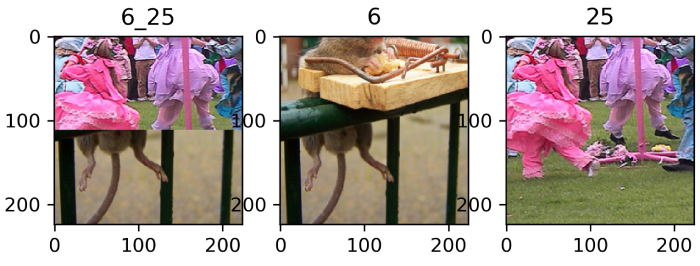
Figure 3: CutMix mixture for image 6 and 25 of Fig. 4. SIM is more sensitive to large color change.

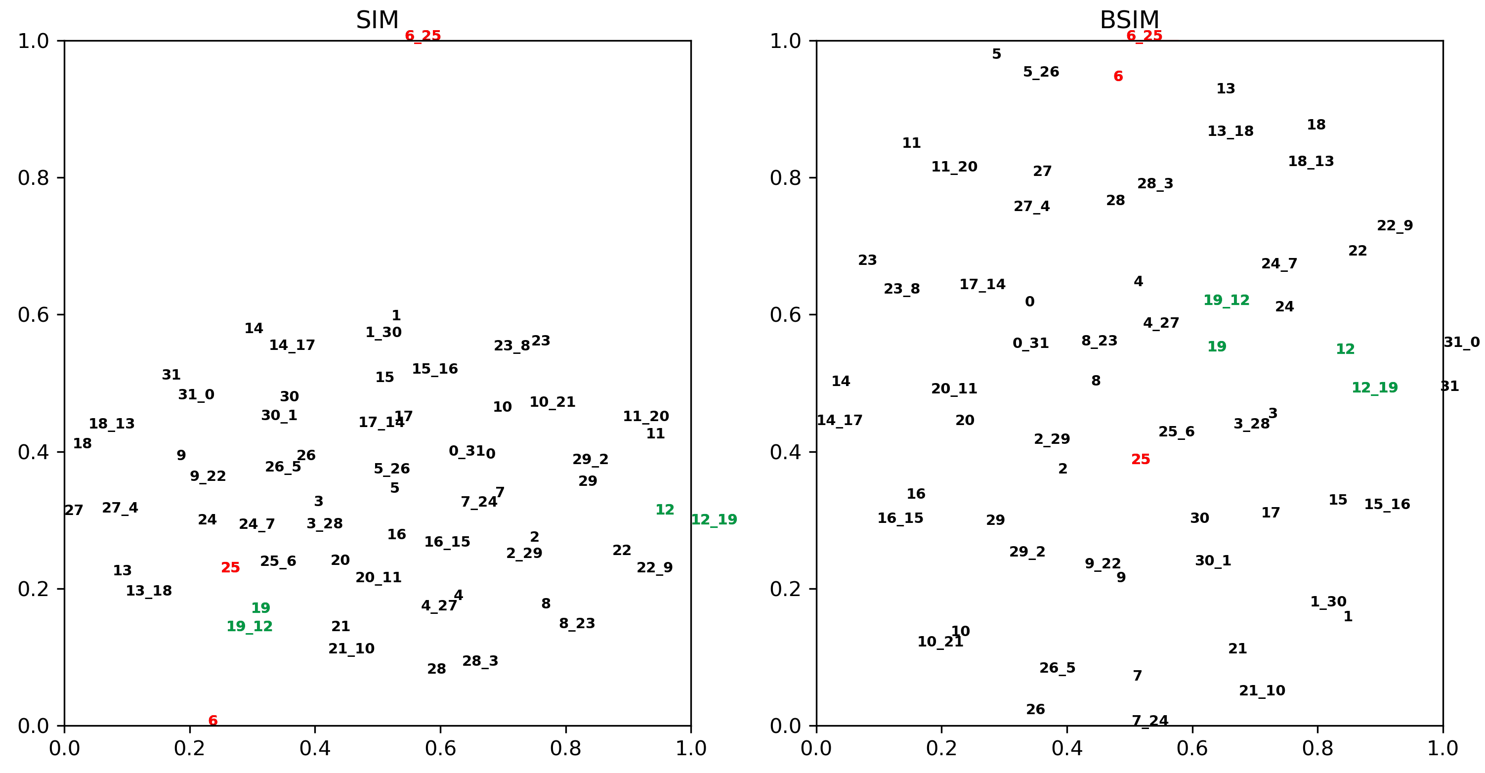
Figure 4: The representation of 2D embeddings using TSNE. We use 32 images and construct the mixture using $i$-th and $31-i$-th images. The mixed embedding is marked by $i\_31-i$. Without BSIM, the embedding cannot make good use of the space (i.e. more crowded). Left: SIM, Right: BSIM. Notice SIM pushes a simple mixture ${\color[rgb]{1,0,0}6\_{25}}$ (red) distant from others, leaving a narrow space and a large amount of unused space. Besides, ${\color[rgb]{0,0.59765625,0.265625}12\_19}$ and ${\color[rgb]{0,0.59765625,0.265625}19\_12}$ (green) should be close but are pushed too far. In contrast, in BSIM all instances are scattered quite evenly, while mixed instances are also better placed near its parents.

Appendix E List of Additional Figures

Figure 5 demonstrates that BSIM has better intra-class discrimination that SIM.

Figure 6 shows the difference of mixed images between Mixup and CutMix, where the latter is perceptually more natural.

Figure 7 illustrates a schematic view of latent sphere where the mixed representation is normalized on the surface.

Figure 8 manifests the schematics of of SimCLR-BSIM.

Figure 10 gives the second implementation of BYOL-BSIM.

Figure 11 depicts the beta distribution given different $\alpha$, where we choose $\alpha$ to have a uniform distribution.

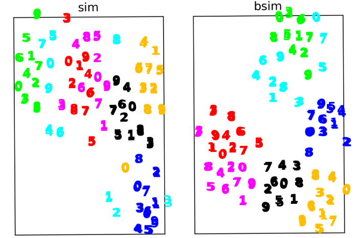
Figure 5: The representation of 2D embeddings using TSNE (sampled 3 times). We draw 10 instances (denoted by number) from each class and make 5 times of data augmentation per instance. The same class are denoted by the same color. BSIM has a better inter-class discrimination than SIM, where instances of the same class are mostly distant from those of other classes.

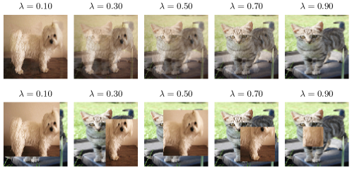
Figure 6: Comparison of Mixup and CutMix with $\lambda$ as the interpolation ratio for Mixup, and cutout ratio for CutMix

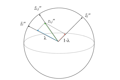
Figure 7: Schematic view of the unit ball in high-dimensional space. The target embedding of the mixed image is $\bar{z}^{\prime\prime}_{i,j}$, which is formed by normalizing $z_{i,j}^{\prime\prime}$ (dashed in green) to the sphere of the unit ball. $z_{i,j}^{\prime\prime}$ is obtained by the $\lambda$ controlled linear interpolation between $z_{i}^{\prime\prime}$ and $z_{j}^{\prime\prime}$.

Figure 8: Adapting BSIM into SimCLR for contrastive learning. Given two images $x_{i}$ and $x_{j}$ (we use $j=N-i$ for speed-up within a batch of N samples), we generate a spurious-positive sample by mixing separately augmented features ($t^{\prime}\sim\mathcal{T}^{\prime}$) into $x_{i,j}^{\prime}$, which pairs with $x_{i}^{\prime\prime}$ and $x_{j}^{\prime\prime}$. SimCLR is a special case of SimCLR-BSIM when $\lambda$ is 0 or 1. Note $f(\cdot)$ is an encoder network and $g(\cdot)$ refers to a projection head, both are trained with the contrastive loss in Equation 1. The representation $\bm{h}$ is later used for downstream tasks.

Figure 10: Applying BSIM to BYOL as in Equation 4. The above blue region is the online network, the below red one is the same target network.

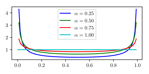
Figure 11: Probability density function of Beta distribution $\beta(\alpha,\alpha)$ under different settings. Notice when $\alpha=1$ we have a uniform distribution.

References

- [Asano et al.(2019)Asano, Rupprecht, and Vedaldi] YM Asano, C Rupprecht, and A Vedaldi. A critical analysis of self-supervision, or what we can learn from a single image. In International Conference on Learning Representations, 2019.
- [Boser et al.(1992)Boser, Guyon, and Vapnik] Bernhard E Boser, Isabelle M Guyon, and Vladimir N Vapnik. A training algorithm for optimal margin classifiers. In Proceedings of the fifth annual workshop on Computational learning theory, pages 144–152, 1992.
- [Caron et al.(2020a)Caron, Misra, Mairal, Goyal, Bojanowski, and Joulin] M. Caron, I. Misra, J. Mairal, Priya Goyal, P. Bojanowski, and Armand Joulin. Unsupervised learning of visual features by contrasting cluster assignments. In Advances in Neural Information Processing Systems, 2020a.
- [Caron et al.(2018)Caron, Bojanowski, Joulin, and Douze] Mathilde Caron, Piotr Bojanowski, Armand Joulin, and Matthijs Douze. Deep clustering for unsupervised learning of visual features. In Proceedings of the European Conference on Computer Vision (ECCV), pages 132–149, 2018.
- [Caron et al.(2020b)Caron, Misra, Mairal, Goyal, Bojanowski, and Joulin] Mathilde Caron, Ishan Misra, Julien Mairal, Priya Goyal, Piotr Bojanowski, and Armand Joulin. Unsupervised learning of visual features by contrasting cluster assignments. Advances in Neural Information Processing Systems, 33, 2020b.
- [Chapelle et al.(2001)Chapelle, Weston, Bottou, and Vapnik] Olivier Chapelle, Jason Weston, Léon Bottou, and Vladimir Vapnik. Vicinal risk minimization. In Advances in neural information processing systems, pages 416–422, 2001.
- [Chen et al.(2020a)Chen, Kornblith, Norouzi, and Hinton] Ting Chen, Simon Kornblith, Mohammad Norouzi, and Geoffrey Hinton. A simple framework for contrastive learning of visual representations. arXiv preprint arXiv:2002.05709, 2020a.
- [Chen and He(2021)] Xinlei Chen and Kaiming He. Exploring simple siamese representation learning. In Proceedings of the IEEE Conference on Computer Vision and Pattern Recognition, 2021.
- [Chen et al.(2020b)Chen, Fan, Girshick, and He] Xinlei Chen, Haoqi Fan, Ross Girshick, and Kaiming He. Improved baselines with momentum contrastive learning. arXiv preprint arXiv:2003.04297, 2020b.
- [Chuang et al.(2020)Chuang, Robinson, Yen-Chen, Torralba, and Jegelka] Ching-Yao Chuang, Joshua Robinson, Lin Yen-Chen, Antonio Torralba, and Stefanie Jegelka. Debiased contrastive learning. arXiv preprint arXiv:2007.00224, 2020.
- [DeVries and Taylor(2017)] Terrance DeVries and Graham W Taylor. Improved regularization of convolutional neural networks with cutout. arXiv preprint arXiv:1708.04552, 2017.
- [Doersch et al.(2015)Doersch, Gupta, and Efros] Carl Doersch, Abhinav Gupta, and Alexei A Efros. Unsupervised visual representation learning by context prediction. In Proceedings of the IEEE international conference on computer vision, pages 1422–1430, 2015.
- [Donahue et al.(2017)Donahue, Krähenbühl, and Darrell] Jeff Donahue, Philipp Krähenbühl, and Trevor Darrell. Adversarial feature learning. In International Conference on Learning Representations, 2017.
- [Dosovitskiy et al.(2014)Dosovitskiy, Springenberg, Riedmiller, and Brox] Alexey Dosovitskiy, Jost Tobias Springenberg, Martin Riedmiller, and Thomas Brox. Discriminative unsupervised feature learning with convolutional neural networks. In Advances in neural information processing systems, pages 766–774, 2014.
- [Everingham et al.(2010)Everingham, Van Gool, Williams, Winn, and Zisserman] Mark Everingham, Luc Van Gool, Christopher KI Williams, John Winn, and Andrew Zisserman. The pascal visual object classes (voc) challenge. International Journal of Computer Vision, 88(2):303–338, 2010.
- [Fan et al.(2008)Fan, Chang, Hsieh, Wang, and Lin] Rong-En Fan, Kai-Wei Chang, Cho-Jui Hsieh, Xiang-Rui Wang, and Chih-Jen Lin. Liblinear: A library for large linear classification. Journal of machine learning research, 9(Aug):1871–1874, 2008.
- [Fisher(1936)] Ronald A Fisher. The use of multiple measurements in taxonomic problems. Annals of eugenics, 7(2):179–188, 1936.
- [Gidaris et al.(2018)Gidaris, Singh, and Komodakis] Spyros Gidaris, Praveer Singh, and Nikos Komodakis. Unsupervised representation learning by predicting image rotations. In International Conference on Learning Representations, 2018. URL https://openreview.net/forum?id=S1v4N2l0-.
- [Girshick et al.(2018)Girshick, Radosavovic, Gkioxari, Dollár, and He] Ross Girshick, Ilija Radosavovic, Georgia Gkioxari, Piotr Dollár, and Kaiming He. Detectron. https://github.com/facebookresearch/detectron, 2018.
- [Gontijo-Lopes et al.(2020)Gontijo-Lopes, Smullin, Cubuk, and Dyer] Raphael Gontijo-Lopes, Sylvia J Smullin, Ekin D Cubuk, and Ethan Dyer. Affinity and diversity: Quantifying mechanisms of data augmentation. arXiv preprint arXiv:2002.08973, 2020.
- [Goyal et al.(2019)Goyal, Mahajan, Gupta, and Misra] Priya Goyal, Dhruv Mahajan, Abhinav Gupta, and Ishan Misra. Scaling and benchmarking self-supervised visual representation learning. In ICCV, pages 6391–6400, 2019.
- [Grill et al.(2020)Grill, Strub, Altché, Tallec, Richemond, Buchatskaya, Doersch, Pires, Guo, Azar, et al.] Jean-Bastien Grill, Florian Strub, Florent Altché, Corentin Tallec, Pierre H Richemond, Elena Buchatskaya, Carl Doersch, Bernardo Avila Pires, Zhaohan Daniel Guo, Mohammad Gheshlaghi Azar, et al. Bootstrap your own latent: A new approach to self-supervised learning. arXiv preprint arXiv:2006.07733, 2020.
- [He et al.(2017)He, Gkioxari, Dollár, and Girshick] Kaiming He, Georgia Gkioxari, Piotr Dollár, and Ross Girshick. Mask r-cnn. In Proceedings of the IEEE international conference on computer vision, pages 2961–2969, 2017.
- [He et al.(2020)He, Fan, Wu, Xie, and Girshick] Kaiming He, Haoqi Fan, Yuxin Wu, Saining Xie, and Ross Girshick. Momentum contrast for unsupervised visual representation learning. In Proceedings of the IEEE/CVF Conference on Computer Vision and Pattern Recognition, pages 9729–9738, 2020.
- [Hénaff et al.(2019)Hénaff, Srinivas, De Fauw, Razavi, Doersch, Eslami, and Oord] Olivier J Hénaff, Aravind Srinivas, Jeffrey De Fauw, Ali Razavi, Carl Doersch, SM Eslami, and Aaron van den Oord. Data-efficient image recognition with contrastive predictive coding. International Conference on Machine Learning, 2019.
- [Iscen et al.(2018)Iscen, Tolias, Avrithis, and Chum] Ahmet Iscen, Giorgos Tolias, Yannis Avrithis, and Ondřej Chum. Mining on manifolds: Metric learning without labels. In Proceedings of the IEEE Conference on Computer Vision and Pattern Recognition (CVPR), June 2018.
- [Kalantidis et al.(2020)Kalantidis, Sariyildiz, Pion, Weinzaepfel, and Larlus] Yannis Kalantidis, Mert Bulent Sariyildiz, Noe Pion, Philippe Weinzaepfel, and Diane Larlus. Hard negative mixing for contrastive learning. In Neural Information Processing Systems (NeurIPS), 2020.
- [Kornblith et al.(2019)Kornblith, Shlens, and Le] Simon Kornblith, Jonathon Shlens, and Quoc V Le. Do better imagenet models transfer better? In Proceedings of the IEEE conference on computer vision and pattern recognition, pages 2661–2671, 2019.
- [Larsson et al.(2017)Larsson, Maire, and Shakhnarovich] Gustav Larsson, Michael Maire, and Gregory Shakhnarovich. Colorization as a proxy task for visual understanding. In Proceedings of the IEEE Conference on Computer Vision and Pattern Recognition, pages 6874–6883, 2017.
- [Lin et al.(2014)Lin, Maire, Belongie, Hays, Perona, Ramanan, Dollár, and Zitnick] Tsung-Yi Lin, Michael Maire, Serge Belongie, James Hays, Pietro Perona, Deva Ramanan, Piotr Dollár, and C Lawrence Zitnick. Microsoft coco: Common objects in context. In European conference on computer vision, pages 740–755. Springer, 2014.
- [Liu et al.(2020)Liu, Zhang, Hou, Wang, Mian, Zhang, and Tang] Xiao Liu, Fanjin Zhang, Zhenyu Hou, Zhaoyu Wang, Li Mian, Jing Zhang, and Jie Tang. Self-supervised learning: Generative or contrastive. arXiv preprint arXiv:2006.08218, 2020.
- [Misra and Maaten(2020)] Ishan Misra and Laurens van der Maaten. Self-supervised learning of pretext-invariant representations. In Proceedings of the IEEE/CVF Conference on Computer Vision and Pattern Recognition, pages 6707–6717, 2020.
- [Noroozi and Favaro(2016)] Mehdi Noroozi and Paolo Favaro. Unsupervised learning of visual representations by solving jigsaw puzzles. In European Conference on Computer Vision, pages 69–84. Springer, 2016.
- [Oord et al.(2018)Oord, Li, and Vinyals] Aaron van den Oord, Yazhe Li, and Oriol Vinyals. Representation learning with contrastive predictive coding. arXiv preprint arXiv:1807.03748, 2018.
- [Owens et al.(2016)Owens, Wu, McDermott, Freeman, and Torralba] Andrew Owens, Jiajun Wu, Josh H McDermott, William T Freeman, and Antonio Torralba. Ambient sound provides supervision for visual learning. In European conference on computer vision, pages 801–816. Springer, 2016.
- [Pathak et al.(2016)Pathak, Krahenbuhl, Donahue, Darrell, and Efros] Deepak Pathak, Philipp Krahenbuhl, Jeff Donahue, Trevor Darrell, and Alexei A Efros. Context encoders: Feature learning by inpainting. In Proceedings of the IEEE conference on computer vision and pattern recognition, pages 2536–2544, 2016.
- [Ren et al.(2015)Ren, He, Girshick, and Sun] Shaoqing Ren, Kaiming He, Ross Girshick, and Jian Sun. Faster r-cnn: Towards real-time object detection with region proposal networks. In Advances in neural information processing systems, pages 91–99, 2015.
- [Shen et al.(2020)Shen, Liu, Liu, Savvides, and Darrell] Zhiqiang Shen, Zechun Liu, Zhuang Liu, Marios Savvides, and Trevor Darrell. Rethinking image mixture for unsupervised visual representation learning. arXiv preprint arXiv:2003.05438, 2020.
- [Thulasidasan et al.(2019)Thulasidasan, Chennupati, Bilmes, Bhattacharya, and Michalak] Sunil Thulasidasan, Gopinath Chennupati, Jeff A Bilmes, Tanmoy Bhattacharya, and Sarah Michalak. On mixup training: Improved calibration and predictive uncertainty for deep neural networks. In Advances in Neural Information Processing Systems, pages 13888–13899, 2019.
- [Tian et al.(2019)Tian, Krishnan, and Isola] Yonglong Tian, Dilip Krishnan, and Phillip Isola. Contrastive multiview coding. arXiv preprint arXiv:1906.05849, 2019.
- [Tian et al.(2020)Tian, Sun, Poole, Krishnan, Schmid, and Isola] Yonglong Tian, Chen Sun, Ben Poole, Dilip Krishnan, Cordelia Schmid, and Phillip Isola. What makes for good views for contrastive learning. arXiv preprint arXiv:2005.10243, 2020.
- [Tokozume et al.(2018a)Tokozume, Ushiku, and Harada] Yuji Tokozume, Yoshitaka Ushiku, and Tatsuya Harada. Between-class learning for image classification. In Proceedings of the IEEE Conference on Computer Vision and Pattern Recognition, pages 5486–5494, 2018a.
- [Tokozume et al.(2018b)Tokozume, Ushiku, and Harada] Yuji Tokozume, Yoshitaka Ushiku, and Tatsuya Harada. Learning from between-class examples for deep sound recognition. In International Conference on Learning Representations, 2018b.
- [Verma et al.(2019)Verma, Lamb, Beckham, Najafi, Mitliagkas, Lopez-Paz, and Bengio] Vikas Verma, Alex Lamb, Christopher Beckham, Amir Najafi, Ioannis Mitliagkas, David Lopez-Paz, and Yoshua Bengio. Manifold mixup: Better representations by interpolating hidden states. In International Conference on Machine Learning, pages 6438–6447. PMLR, 2019.
- [Wang and Isola(2020)] Tongzhou Wang and Phillip Isola. Understanding contrastive representation learning through alignment and uniformity on the hypersphere. In International Conference on Machine Learning, 2020.
- [Wang and Hebert(2016)] Yu-Xiong Wang and Martial Hebert. Learning to learn: Model regression networks for easy small sample learning. In European Conference on Computer Vision, pages 616–634. Springer, 2016.
- [Wu et al.(2020)Wu, Zhuang, Mosse, Yamins, and Goodman] M. Wu, Chengxu Zhuang, M. Mosse, D. Yamins, and Noah D. Goodman. On mutual information in contrastive learning for visual representations. ArXiv, abs/2005.13149, 2020.
- [Wu et al.(2019)Wu, Kirillov, Massa, Lo, and Girshick] Yuxin Wu, Alexander Kirillov, Francisco Massa, Wan-Yen Lo, and Ross Girshick. Detectron2. https://github.com/facebookresearch/detectron2, 2019.
- [Wu et al.(2018)Wu, Xiong, Stella, and Lin] Zhirong Wu, Yuanjun Xiong, X Yu Stella, and Dahua Lin. Unsupervised feature learning via non-parametric instance discrimination. In Proceedings of the IEEE Conference on Computer Vision and Pattern Recognition, 2018.
- [Xie et al.(2020)Xie, Zhan, Liu, Ong, and Loy] Jiahao Xie, Xiaohang Zhan, Z. Liu, Y. S. Ong, and Chen Change Loy. Delving into inter-image invariance for unsupervised visual representations. ArXiv, abs/2008.11702, 2020.
- [You et al.(2017)You, Gitman, and Ginsburg] Yang You, Igor Gitman, and Boris Ginsburg. Scaling sgd batch size to 32k for imagenet training. arXiv preprint arXiv:1708.03888, 6, 2017.
- [Yun et al.(2019)Yun, Han, Oh, Chun, Choe, and Yoo] Sangdoo Yun, Dongyoon Han, Seong Joon Oh, Sanghyuk Chun, Junsuk Choe, and Youngjoon Yoo. Cutmix: Regularization strategy to train strong classifiers with localizable features. In Proceedings of the IEEE International Conference on Computer Vision, pages 6023–6032, 2019.
- [Zhai et al.(2019a)Zhai, Oliver, Kolesnikov, and Beyer] Xiaohua Zhai, Avital Oliver, Alexander Kolesnikov, and Lucas Beyer. S4l: Self-supervised semi-supervised learning. In Proceedings of the IEEE international conference on computer vision, pages 1476–1485, 2019a.
- [Zhai et al.(2019b)Zhai, Puigcerver, Kolesnikov, Ruyssen, Riquelme, Lucic, Djolonga, Pinto, Neumann, Dosovitskiy, et al.] Xiaohua Zhai, Joan Puigcerver, Alexander Kolesnikov, Pierre Ruyssen, Carlos Riquelme, Mario Lucic, Josip Djolonga, Andre Susano Pinto, Maxim Neumann, Alexey Dosovitskiy, et al. A large-scale study of representation learning with the visual task adaptation benchmark. arXiv preprint arXiv:1910.04867, 2019b.
- [Zhan et al.(2020a)Zhan, Xie, Liu, Ong, and Loy] Xiaohang Zhan, Jiahao Xie, Ziwei Liu, Yew-Soon Ong, and Chen Change Loy. Online deep clustering for unsupervised representation learning. In Proceedings of the IEEE/CVF Conference on Computer Vision and Pattern Recognition, pages 6688–6697, 2020a.
- [Zhan et al.(2020b)Zhan, Xie, and Xie] Xiaohang Zhan, Jiahao Xie, and Enze Xie. OpenSelfSup. https://github.com/open-mmlab/OpenSelfSup, 2020b.
- [Zhang et al.(2018)Zhang, Cisse, Dauphin, and Lopez-Paz] Hongyi Zhang, Moustapha Cisse, Yann N Dauphin, and David Lopez-Paz. mixup: Beyond empirical risk minimization. In International Conference on Learning Representations, 2018.
- [Zhang et al.(2017)Zhang, Isola, and Efros] Richard Zhang, Phillip Isola, and Alexei A Efros. Split-brain autoencoders: Unsupervised learning by cross-channel prediction. In Proceedings of the IEEE Conference on Computer Vision and Pattern Recognition, pages 1058–1067, 2017.
- [Zhuang et al.(2019)Zhuang, Zhai, and Yamins] Chengxu Zhuang, Alex Lin Zhai, and Daniel Yamins. Local aggregation for unsupervised learning of visual embeddings. In Proceedings of the IEEE International Conference on Computer Vision, pages 6002–6012, 2019.