Describing the Migdal effect with a bremsstrahlung-like process and many-body effects

Abstract

Recent theoretical studies have suggested that the suddenly recoiled atom struck by dark matter (DM) particle is much more likely to excite or lose its electrons than expected. Such Migdal effect opens a new avenue for exploring the sub-GeV DM particles. There have been various attempts to describe the Migdal effect in liquid and semiconductor targets. In this paper we incorporate the treatment of the bremsstrahlung process and the electronic many-body effects to give a full description of the Migdal effect in bulk semiconductor targets diamond and silicon. Compared with the results obtained with the atom-centered localized Wannier functions (WFs) under the framework of the tight-binding (TB) approximation, the method proposed in this study yields much larger event rates in the low energy regime, due to a $\omega^{-4}$ scaling. We also find that the effect of the bremsstrahlung photon mediating the Coulomb interaction between recoiled ion and the electron-hole pair is equivalent to that of the exchange of a single phonon.

I Introduction

Although there has been overwhelming evidence for the existence of the dark matter (DM) from astrophysics and cosmology, its particle nature still remains mysterious. In the past decades, tremendous efforts have been invested into the search of the weakly interacting massive particles (WIMPs), one of the most promising DM candidate, but conclusive evidence has not yet emerged. Owing to the continuous developments in detector technologies in recent years, the frontier of the dark matter direct detection has been pushed to the mass range below the GeV scale, where the traditional detection methods based on the nuclear scattering are expected to lose sensitivity. So more and more theorists and experimentalists have begun to shift to other alternative proposals based on new detection channels and materials, such as with semiconductors [1, 2, 3, 4], Dirac materials [5, 6, 7], superconductors [8, 9], superfluid helium [10, 11, 12], and via phonon excitations [13, 14, 15] and bremsstrahlung photons [16, 17], as well as other proposals and analyses [18, 19, 20, 21, 22, 23, 24, 25, 26, 27, 28, 29, 30, 31, 32, 33, 34, 35, 36, 37, 38].

The Migdal effect has aroused wide interest recently because it is theoretically clarified that the suddenly struck nucleus can produce ionized electrons more easily than anticipated for an incident sub-GeV DM particle [39], so exploring the sub-GeV parameter space is possible for the present detection technologies. There has been numerous theoretical proposals [40, 41, 42, 43, 44] and experimental efforts [45, 46, 47] dedicated to detecting sub-GeV DM particles via the Migdal effect. Ref. [48] first investigated the Migdal effect in semiconductor targets by exploring the connection between the DM-electron scattering in semiconductors and Migdal processes in isolated atoms. In our previous study [42], we proposed to describe the Migdal effect in semiconductors under the framework of the tight-binding (TB) approximation, where a Galilean boost operator is imposed on the recoiled ion to account for the highly local impulsive effect brought by the incident DM particle, while the extensive nature of the electrons in solids is reflected in the hopping integrals.

Meanwhile, nontrivial collective behavior in condensed matter system has also attracted attention and has been considered as a possible origin of observed signal features in various experiments [49]. Ref. [49] put forward two mechanisms based on the plasmon production induced by DM particles to explain the existing signal lineshapes that are at odds with the standard interpretations of the DM-electron scattering. As a typical many-body phenomenon in solids, the plasmon excitation cannot be understood in terms of standard two-body scattering, or non-interacting single-particle states. Therefore, the many-body physics may shed new light on the interpretation of the DM-detector interactions.

On the other hand, Ref. [50] examined the above postulates by concretely calculating the bremsstrahlung emission of plasmon induced indirectly by a DM particle. While the many-body effect, namely, the plasmon resonance can be well described in the same way as in the electron energy loss spectroscopy (EELS) analysis, the effect of a fast charged electron transversing the material is replaced with an abruptly recoiling ion, and this part of physics can be summarized with the bremsstrahlung-like process, in the context of classical electrodynamics or quantum mechanics.

In this study we integrate above two aspects, i.e., the electronic many-body effect and the bremsstrahlung-like description of the recoiled ion, into a coherent method to describe the Migdal effect in solids. In this picture the suddenly recoiled ion excites a primary electron-hole pair via the bremsstrahlung photon, while the many-body physics is encoded in the dielectric function $\epsilon\left(\mathbf{k},\omega\right)$, which is responsible for the screening of the pure Coulomb interaction and the emergence of collective plasma oscillations. It is tempting to investigate the consequence of the many-body physics on the DM semiconductor detector. In order to take into account the local field effect, the calculation of $\epsilon\left(\mathbf{k},\omega\right)$ is extended to the case in crystalline environment using the random phase approximation (RPA). Based on this method, we concretely estimate the Migdal excitation event rates in bulk diamond and silicon semiconductors, respectively. Moreover, considering there have existed other methods describing the Migdal effect in solids, such as the aforementioned TB approximation, thus we also make comparisons with the event rates obtained from the TB approximation, or the atom-centered Wannier functions (WFs) [42].

This paper is organized as follows. We begin Sec. II by giving the quantum mechanical formalism and relevant scheme for calculating the Migdal excitation event rates induced by DM particles. Based on this approach, we then specifically calculate the event rates for diamond and silicon semiconductors, respectively in Sec. III. We conclude and make some comments on the methodology in Sec. IV. Some details of the derivation in the main text are provided in the Appendices.

II Electronic excitation in the quantum field theory description

We begin this section with a short review of the description of the Migdal effect in crystal structures in the context of the quantum theory.

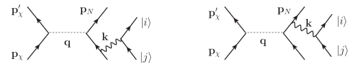
Figure 1: The diagrams of the process $\chi\left(p_{\chi}\right)+N\rightarrow\chi\left(p_{\chi}^{\prime}\right)+N\left(p_{N}\right)+h\left(j\right)+e\left(i\right)$.

II.1 A general formula for Migdal effect in quantum field theory

The Migdal effect in solids refers to the process in which the incident DM particle collides with a nucleus in crystal, and the recoiled nucleus excites an electron across the band gap from valence state $\ket{j}$ to a conduction state $\ket{i}$. As has been pointed out in our previous study [42] that the boost argument for the Migdal effect in an isolated atom used in Ref. [39] no longer applies for the crystalline solids, because one can not regard the whole crystal target as a big nucleus: it is the struck nucleus in the crystal that is recoiling, but not the whole crystal. A description fixed to the crystal is preferred. Inspired by the treatment of the plasmon production in Ref. [50], in this study we discuss the Migdal effect with similar description in the hope that sudden acceleration effect of the nucleus will be well captured with a bremsstrahlung-like process. This process can also be understood as the two-body scattering between the DM particle and a nucleus, with the scattered DM particle and the nucleus, as well as the electron-hole pair as the final states, i.e., the process $\chi\left(p_{\chi}\right)+N\rightarrow\chi\left(p_{\chi}^{\prime}\right)+N\left(p_{N}\right)+\,$electron-hole pair, where $\chi$ stands for the DM particle, $N\left(p_{N}\right)$ $\left(N\left(p_{N}^{\prime}\right)\right)$ is the nucleus before (after) the collision. The relevant Feynman diagrams are presented in Fig. 1, where $e\left(i\right)$ and $h\left(j\right)$ represent the electronic conduction and valence states, respectively, from which the amplitude is read as

$$i\mathcal{M} = \sum_{\mathbf{k}}\frac{\left(-i\right)}{V}V_{\chi N}\left(\mathbf{q}\right)\,V_{Ne}\left(\mathbf{k}\right)\>\braket{i}{e^{i\mathbf{k}\cdot\hat{\mathbf{x}}}}{j}$$ (1)

$$\times \left[\frac{1}{\frac{p_{N}^{2}}{2m_{N}}+\varepsilon_{ij}-\frac{\left|\mathbf{p}_{N}+\mathbf{k}\right|^{2}}{2m_{N}}}-\frac{1}{\varepsilon_{ij}+\frac{k^{2}}{2m_{N}}}\right],$$

where $\mathbf{q}=-\mathbf{p}_{N}-\mathbf{k}$, $p_{N}=\left|\mathbf{p}_{N}\right|$, $k=\left|\mathbf{k}\right|$, $V$ is the volume of the crystal, $m_{N}$ is the nucleus mass, $\varepsilon_{ij}=\varepsilon_{i}-\varepsilon_{j}$ is the energy difference between the conduction states $\left\{\ket{i}\right\}$ and valence states $\left\{\ket{j}\right\}$, $V_{\chi N}\left(\mathbf{q}\right)$ represents the DM-nucleus contact interaction $V_{\chi N}\left(\mathbf{x}\right)$ in momentum space, which is connected to the DM-nucleus cross section with the following relation,

$$\left|V_{\chi N}\left(\mathbf{q}\right)\right|^{2} = \left|\int\mathrm{d}^{3}x\,e^{-i\mathrm{\mathbf{q}\cdot\mathbf{x}}}\,V_{\chi N}\left(\mathbf{x}\right)\right|^{2}$$ (2)

$$= \frac{A^{2}\pi\sigma_{\chi n}}{\mu_{\chi n}^{2}},$$

where $A$ is the atomic number of the target nucleus, $\sigma_{\chi n}$ and $\mu_{\chi n}=m_{n}\,m_{\chi}/\left(m_{n}+m_{\chi}\right)$ represent the cross section and the reduced mass of the DM-nucleon pair, respectively. $V_{Ne}\left(\mathbf{k}\right)$ is the ion-electron Coulomb interaction propagator

$$V_{Ne}\left(\mathbf{k}\right) = \int\mathrm{d}^{3}x\,e^{-i\mathrm{\mathbf{k}\cdot\mathbf{x}}}\,\frac{Z_{\mathrm{ion}}e^{2}}{4\pi\,\left|\mathbf{x}\right|}$$ (3)

$$= \frac{Z_{\mathrm{ion}}4\pi\alpha}{k^{2}},$$

where $Z_{\mathrm{ion}}$ is the number of valence electrons, and $\alpha$ is the fine structure constant. In the soft limit where $\mathbf{p}_{N}\cdot\mathbf{k}/m_{N}\ll\varepsilon_{ij}$ and $\left|\mathbf{k}\right|\ll\left|\mathbf{p}_{N}\right|$, the nucleus propagator in Eq. (1) can be simplified as [50]

$$\frac{1}{\frac{p_{N}^{2}}{2m_{N}}+\varepsilon_{ij}-\frac{\left|\mathbf{p}_{N}+\mathbf{k}\right|^{2}}{2m_{N}}}-\frac{1}{\varepsilon_{ij}+\frac{k^{2}}{2m_{N}}} \simeq \left(\frac{\mathbf{p}_{N}\cdot\mathbf{k}}{m_{N}}\right)\frac{1}{\varepsilon_{ij}^{2}}.$$

At this stage, one may wonder, whether the bremsstrahlung-like process (where an electron is excited via exchanging a photon) amounts to a complete description of the actual physical process, considering that in discussion of the Migdal effect in an isolated atom, the excitation process is described with a full evolution of the Hamiltonian. So if one can show that bremsstrahlung-like description is equivalent to the boost argument for the Migdal effect in an isolated atom, the bremsstrahlung-like narrative can be convincingly generalized to the crystalline solids. To this end, we apply above discussion to an isolated atom by substituting the valence ($\ket{j}$) and conduction ($\ket{i}$) states, as well as the valence charge $Z_{\mathrm{ion}}$, with initial ($\ket{\alpha}$), final  ($\ket{\beta}$) atomic states, and the atomic effective charge $Z_{\mathrm{eff}}$, respectively, and the amplitude in Fig. 1 can be read off as the following,

$$i\mathcal{M} = \left(-i\right)V_{\chi N}\left(\mathbf{q}\right)\,\int\frac{\mathrm{d}^{3}k}{\left(2\pi\right){}^{3}}\frac{Z_{\mathrm{eff}}\,4\pi\alpha}{k^{2}}\>\braket{\beta}{e^{i\mathbf{k}\cdot\hat{\mathbf{x}}}}{\alpha}$$ (5)

$$\times\frac{\mathbf{v}_{N}\cdot\mathbf{k}}{\left(E_{\beta}-E_{\alpha}\right)^{2}},$$

where $\mathbf{v}_{N}=\mathbf{p}_{N}/m_{N}$ represents the velocity of the recoiled atom, and the correspondence $\frac{1}{V}\sum_{\mathbf{k}}\sim\int\frac{\mathrm{d}^{3}k}{\left(2\pi\right){}^{3}}$ is used. On the other hand, as demonstrated in Ref. [51] that the excitation rate derived with the boost argument in Ref. [39] is connected to above bremsstrahlung-like approach through the relation

$$\braket{\beta}{e^{im_{e}\mathbf{v}_{N}\cdot\hat{\mathbf{x}}}}{\alpha}\simeq im_{e}\mathbf{v}_{N}\cdot\braket{\beta}{\hat{\mathbf{x}}}{\alpha}$$

$$=\frac{Z_{\mathrm{eff}}\,4\pi\alpha}{\left(E_{\beta}-E_{\alpha}\right)^{2}}\int\frac{\mathrm{d}^{3}k}{\left(2\pi\right){}^{3}}\frac{\mathbf{v}_{N}\cdot\mathbf{k}}{k^{2}}\braket{\beta}{e^{i\mathbf{k}\cdot\hat{\mathbf{x}}}}{\alpha},$$ (6)

where $m_{e}$ is the electron mass, and $E_{\alpha}$ ($E_{\beta}$) is the energy of the initial (final) state. Thus the bremsstrahlung-like framework can also describe the Migdal effect in an isolated atom. At first sight, one may conclude that this relation also holds in solids, and hence the atomic formulation can be directly generalized to the semiconductors [48, 44]. However, this is not true because the derivation of Eq. (6) rests on a central Coulomb potential $-Z_{\mathrm{eff}}e^{2}/r$, while in the crystalline environment the itinerant electrons are also subjected to the Coulomb interaction from all neighboring ions, and thus such generalization is invalid. In contrast, our rationale is that, since the bremsstrahlung-like narrative has been justified in the case of isolated atoms, we generalize this description to the case in semiconductors, which leads to Eq. (1), rather than $\braket{i}{e^{im_{e}\mathbf{v}_{N}\cdot\hat{\mathbf{x}}}}{j}$.

Moreover, if one takes into consideration the screening effect by introducing the dielectric function $\epsilon^{-1}\left(\mathbf{k},\omega\right)$ [49], the total event rate for the DM flux impinging on a semiconductor and then exciting a primary electron-hole pair can be written as:

$$R = \frac{\rho_{\chi}}{m_{\chi}}N_{T}\left\langle\sigma v\right\rangle$$ (7)

$$= \frac{\rho_{\chi}}{m_{\chi}}\frac{4\pi^{2}A^{2}\sigma_{\chi n}\,Z_{\mathrm{ion}}^{2}\,\alpha\,N_{T}}{3\,\mu_{\chi n}^{2}\,\left(2\pi\right)^{6}}\int\mathrm{d^{3}}v\frac{f_{\chi}\left(\mathbf{v}\right)}{v}\int\mathrm{d}^{3}p_{N}\frac{\left|\mathbf{v}_{\mathrm{ion}}\right|^{2}}{p_{N}}$$

$$\times\int\frac{\mathrm{d}\omega}{\omega^{4}}\varTheta\left[v-v_{\mathrm{min}}\left(p_{N},\,\omega\right)\right]\int\mathrm{d}^{3}k\frac{2\times 4\pi^{2}\alpha}{V\,k^{2}\left|\epsilon\left(\mathbf{k},\omega\right)\right|^{2}}$$

$$\times\sum_{i,\,j}\left|\braket{i}{e^{i\mathbf{k}\cdot\hat{\mathbf{x}}}}{j}\right|^{2}\,\delta\left(\varepsilon_{i}-\varepsilon_{j}-\omega\right),$$

where the bracket $\left\langle\cdots\right\rangle$ denotes the average over the DM velocity distribution, $\rho_{\chi}$ represents the DM local density, $N_{T}$ is number of the nuclei in target, $f_{\chi}\left(\mathbf{v}\right)$ is the DM velocity distribution, $\mathbf{v}_{\mathrm{ion}}=\mathbf{p}_{N}/m_{N}$ is the velocity of the recoiled nucleus, $\omega$ denotes the relevant energy difference, and $\Theta$ is the Heaviside step function; the factor $1/3$ stems from the average over all directions of $\mathbf{k}$, given the isotropic nature of the electron gas; in the last line the factor $2$ counts the two degenerate spin states. For the given $p_{N}$ and $\omega$, function $v_{\mathrm{min}}$ determines the minimum kinetically accessible velocity for the transition:

$$v_{\mathrm{min}}\left(p_{N},\,\omega\right) = \frac{p_{N}}{2\,\mu_{\chi N}}+\frac{\omega}{p_{N}},$$ (8)

with $\mu_{\chi N}=m_{N}\,m_{\chi}/\left(m_{N}+m_{\chi}\right)$ being the reduced mass of the DM-nucleus pair. In practice, we take $\rho_{\chi}=0.3\,\mathrm{GeV/cm^{3}}$, and the velocity distribution can be approximated as a truncated Maxwellian form in the Galactic rest frame, i.e., $f_{\chi}\left(\mathbf{v}\right)\propto\exp\left[-\left|\mathbf{v}+\mathbf{v}_{\mathrm{e}}\right|^{2}/v_{0}^{2}\right]\,\Theta\left(v_{\mathrm{esc}}-\left|\mathbf{v}+\mathbf{v}_{\mathrm{e}}\right|\right)$, with the Earth’s velocity $v_{\mathrm{e}}=230\,\mathrm{km/s}$, the dispersion velocity $v_{0}=220\,\mathrm{km/s}$ and the Galactic escape velocity $v_{\mathrm{esc}}=544\,\,\mathrm{km/s}$.

II.2 Migdal effect with random phase approximation

As illustrated in general expression of the Migdal event rate Eq. (7), the dielectric function $\epsilon^{-1}\left(\mathbf{k},\omega\right)$ plays the central role in the estimate, accounting for the many-body effects. In this paper we calculate the dielectric function with the random phase approximation (RPA), which corresponds to the Lindhard formula:

$$\mathrm{Im}\left[\epsilon\left(\mathbf{k},\omega\right)\right] \simeq 2\times\frac{4\pi^{2}\alpha}{V\,k^{2}}\,\sum_{i,\,j}\left|\braket{i}{e^{i\mathbf{k}\cdot\hat{\mathbf{x}}}}{j}\right|^{2}\,\delta\left(\varepsilon_{i}-\varepsilon_{j}-\omega\right),$$ (9)

with which the total event rate including the electronic many-body effect is recast as follows

$$R = \frac{\rho_{\chi}}{m_{\chi}}\frac{4\pi^{2}A^{2}\sigma_{\chi n}\,Z_{\mathrm{ion}}^{2}\,\alpha\,N_{T}}{3\,\mu_{\chi n}^{2}\,\left(2\pi\right)^{6}}\int\mathrm{d^{3}}v\frac{f_{\chi}\left(\mathbf{v}\right)}{v}\int\mathrm{d}^{3}p_{N}\frac{\left|\mathbf{v}_{\mathrm{ion}}\right|^{2}}{p_{N}}\int\frac{\mathrm{d}\omega}{\omega^{4}}\varTheta\left[v-v_{\mathrm{min}}\left(p_{N},\,\omega\right)\right]\int\mathrm{d}^{3}k\,\mathrm{Im}\left[\frac{-1}{\epsilon\left(\mathbf{k},\omega\right)}\right].$$ (10)

This formula applies for the textbook model for the homogeneous electron gas. In crystalline structure the translational symmetry for spacetime reduces to that for the periodic crystal lattice. In this case, above expression is rewritten as the following:

$$R = \frac{\rho_{\chi}}{m_{\chi}}\frac{4\pi^{2}A^{2}\sigma_{\chi n}\,Z_{\mathrm{ion}}^{2}\,\alpha\,N_{T}}{3\,\mu_{\chi n}^{2}\,\left(2\pi\right)^{3}\Omega}\int\mathrm{d^{3}}v\,\frac{f_{\chi}\left(\mathbf{v}\right)}{v}\int\mathrm{d}^{3}p_{N}\frac{\left|\mathbf{v}_{\mathrm{ion}}\right|^{2}}{p_{N}}\int\frac{\mathrm{d}\omega}{\omega^{4}}\,\varTheta\left[v-v_{\mathrm{min}}\left(p_{N},\,\omega\right)\right]\mathcal{F}\left(\omega\right)$$ (11)

$$= \frac{\rho_{\chi}}{m_{\chi}}\frac{2\,A^{2}\sigma_{\chi n}\,Z_{\mathrm{ion}}^{2}\,\alpha\,N_{T}}{3\,\mu_{\chi n}^{2}\,\Omega\,m_{N}^{2}}\int\mathrm{d^{3}}v\,\frac{f_{\chi}\left(\mathbf{v}\right)}{v}\int p{}_{N}^{3}\,\mathrm{d}p_{N}\int\frac{\mathrm{d}\omega}{\omega^{4}}\,\varTheta\left[v-v_{\mathrm{min}}\left(p_{N},\,\omega\right)\right]\mathcal{F}\left(\omega\right),$$

where the nondimensional factor

$$\mathcal{F}\left(\omega\right) = \sum_{\mathbf{G},\mathbf{G}^{\prime}}\int_{1\mathrm{BZ}}\frac{\varOmega\,\mathrm{d}^{3}\left[k\right]}{\left(2\pi\right)^{3}}\,\frac{\left(\left[\mathbf{k}\right]+\mathbf{G}\right)\cdot\left(\left[\mathbf{k}\right]+\mathbf{G}^{\prime}\right)}{\left|\left[\mathbf{k}\right]+\mathbf{G}\right|\left|\left[\mathbf{k}\right]+\mathbf{G}^{\prime}\right|}\,\mathrm{Im}\left[-\widetilde{\epsilon}_{\mathbf{G},\mathbf{G}^{\prime}}^{-1}\left(\mathbf{\left[k\right]},\omega\right)\right]$$ (12)

represents the averaged energy loss function, with $\Omega$ being the volume of the unit cell. The transferred momentum $\mathbf{k}$ in Eq. (10) is expressed uniquely as the sum of a reciprocal lattice vector $\mathbf{G}$, and corresponding reduced momentum $\left[\mathbf{k}\right]$ confined in the first BZ, i.e., $\mathbf{k}=\left[\mathbf{k}\right]+\mathbf{G}$. $\mathcal{F}\left(\omega\right)$ can be obtained from inverting the microscopic dielectric matrix

$$\widetilde{\epsilon}_{\mathbf{G},\mathbf{G}^{\prime}}\left(\mathbf{\left[\mathbf{k}\right]},\omega\right) = \delta_{\mathbf{G},\mathbf{G}^{\prime}}-\frac{1}{V}\frac{4\pi\alpha}{\left|\mathbf{\left[\mathbf{k}\right]}+\mathbf{G}\right|\left|\mathbf{\left[\mathbf{k}\right]}+\mathbf{G}^{\prime}\right|}\sum_{i,j}\frac{\braket{i}{e^{i\left(\mathbf{\mathbf{\mathbf{\left[\mathbf{k}\right]}+\mathbf{G}}}^{\prime}\right)\cdot\hat{\mathbf{x}}}}{j}\braket{j}{e^{-i\left(\mathbf{\mathbf{\left[\mathbf{k}\right]+\mathbf{G}}}\right)\cdot\hat{\mathbf{x}}}}{i}}{\varepsilon_{ij}-\omega-i0^{+}}\left(n_{i}-n_{j}\right),$$ (13)

where $n_{i}$ ($n_{j}$) denotes the occupation number of the state $\ket{i}$ ($\ket{j}$). The non-vanishing $\mathbf{G}$-vectors in the microscopic dielectric matrix reflect the variation of the microscopic field over a unit cell. For simplicity, the crystal structure is still approximated as isotropic in discussion. If one presumes that the fine structure constant $\alpha$ well suppresses the matrix elements, and then takes only the terms up to the first order in the resolvent $\left(I-M\right)^{-1}=I+M+M^{2}+\cdots$, where the identity matrix $I$ and $M$ represent the first and the the second terms in Eq. (13), respectively, the inverse matrix can be approximated as

$$\tilde{\epsilon}_{\mathbf{G},\mathbf{G}^{\prime}}^{-1}\left(\mathbf{\mathbf{\left[\mathbf{k}\right]}},\omega\right) \simeq \delta_{\mathbf{G},\mathbf{G}^{\prime}}+\frac{1}{V}\frac{4\pi\alpha}{\left|\mathbf{\left[\mathbf{k}\right]}+\mathbf{G}\right|\left|\mathbf{\left[\mathbf{k}\right]}+\mathbf{G}^{\prime}\right|}\sum_{i,j}\frac{\braket{i}{e^{i\left(\mathbf{\mathbf{\mathbf{\left[\mathbf{k}\right]}+\mathbf{G}}}^{\prime}\right)\cdot\hat{\mathbf{x}}}}{j}\braket{j}{e^{-i\left(\mathbf{\mathbf{\mathbf{\left[\mathbf{k}\right]}+\mathbf{G}}}\right)\cdot\hat{\mathbf{x}}}}{i}}{\varepsilon_{ij}-\omega-i0^{+}}\left(n_{i}-n_{j}\right),$$ (14)

and hence

$$\mathrm{Im}\left[-\tilde{\epsilon}_{\mathbf{G},\mathbf{G}^{\prime}}^{-1}\left(\mathbf{\mathbf{\left[\mathbf{k}\right]}},\omega\right)\right] \simeq \frac{2}{V}\frac{4\pi^{2}\alpha}{\left|\mathbf{\left[\mathbf{k}\right]}+\mathbf{G}\right|\left|\mathbf{\left[\mathbf{k}\right]}+\mathbf{G}^{\prime}\right|}\,\sum_{i,\,j}\braket{i}{e^{i\left(\mathbf{\mathbf{\mathbf{\left[\mathbf{k}\right]}+\mathbf{G}}}^{\prime}\right)\cdot\hat{\mathbf{x}}}}{j}\braket{j}{e^{-i\left(\mathbf{\mathbf{\mathbf{\left[\mathbf{k}\right]}+\mathbf{G}}}\right)\cdot\hat{\mathbf{x}}}}{i}\,\delta\left(\varepsilon_{i}-\varepsilon_{j}-\omega\right),$$ (15)

which exactly corresponds to the case without the screening effect. In this study the inverse matrix is calculated in a straightforward way.

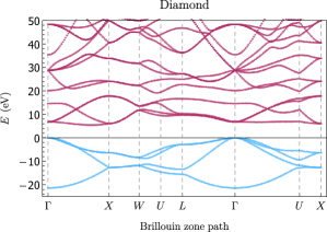
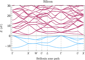
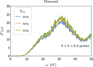
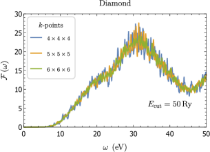
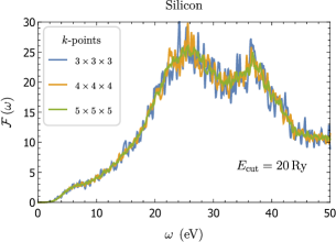
Figure 2: Top: The scissor-corrected band structure of bulk diamond (left) and silicon (right) obtained from DFT calculation, with the band gap $E_{g}=5.47\,\mathrm{eV}$ ($1.12\,\mathrm{eV}$). Middle: Given the 6$\times$6$\times$6 (5$\times$5$\times$5) $k$-point mesh for diamond (left) and silicon (right), the energy loss spectra $\mathcal{F}\left(\omega\right)$ introduced in Eq. (13), for $E_{\mathrm{cut}}=10\,\mathrm{Ry}$ ($6\,\mathrm{Ry}$), $20\,\mathrm{Ry}$ ($10\,\mathrm{Ry}$), and $50\,\mathrm{Ry}$ ($20\,\mathrm{Ry}$), respectively. Bottom: Given $E_{\mathrm{cut}}=50\,\mathrm{Ry}$ ($20\,\mathrm{Ry}$) for diamond (left) and silicon (right), the spectrum $\mathcal{F}\left(\omega\right)$ for the 6$\times$6$\times$6 (5$\times$5$\times$5), 5$\times$5$\times$5 (4$\times$4$\times$4), and 4$\times$4$\times$4 (3$\times$3$\times$3) $k$-point mesh, respectively. See text for details.

III Computational details and results

Now we are in a position to put into practice the estimate of the Migdal excitation event rate. With $\mathtt{Quantum\>Espresso}$ package [52] plus a norm-conserving pseudopotential [53], we perform the density functional theory (DFT) calculation to obtain the Bloch eigenfunctions and eigenvalues using the local-density approximation [54] for the exchange-correlation functional, on a uniform $6\times 6\times 6$ ($5\times 5\times 5$) $k$-point mesh for diamond (silicon) via the Monkhorst-Pack [55] scheme. A core cutoff radius of $1.3\,\mathrm{Bohr}$ ($1.8\,\mathrm{Bohr}$) is adopted and the outermost four electrons are treated as valence for diamond (silicon). The energy cut $\varepsilon_{\mathrm{cut}}$ is set to $200\,\mathrm{Ry}$ ($70\,\mathrm{Ry}$) and lattice constant 3.577 Å  (5.429 Å) for diamond (silicon) obtained from experimental data is adopted. The band structure of diamond (silicon) crystal is presented in the upper left (right) panel of Fig. 2, where the scissor correction is conducted to match the experimental value of the band gap $E_{g}=5.47\,\mathrm{eV}$ ($1.12\,\mathrm{eV}$).

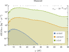
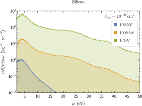
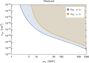
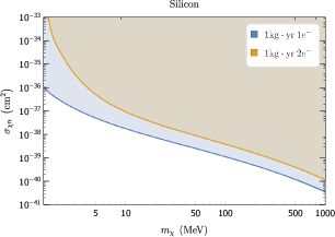
Figure 3: Top: The differential Migdal electronic excitation event rate in crystalline diamond (left) and silicon (right), calculated at the RPA level for the reference values $\sigma_{\chi n}=10^{-38}\,\mathrm{cm}^{2}$ and $m_{\chi}=10\,\mathrm{MeV}$ (blue), $100\,\mathrm{MeV}$(orange) and $1\,\mathrm{GeV}$ (green), respectively. Bottom: Relevant cross-section sensitivities for the Migdal effect at 90% C.L. for a 1 kg-yr diamond (left) and silicon (right) detector, based on the single-electron (blue) and the two-electron (orange) bin data, respectively. See text for details.

The matrix $\epsilon_{\mathbf{G},\mathbf{G}^{\prime}}^{-1}$ is calculated via directly inverting the matrix Eq. (13) with the $\mathtt{YAMBO}$ code [56, 57], with a smaller matrix cutoff $E_{\mathrm{cut}}$ of $50\,\mathrm{Ry}$ ($20\,\mathrm{Ry}$) for diamond (silicon). An energy bin width $\Delta\omega=0.05\,\mathrm{eV}$ is adopted within the range from $0$ to $50\,\mathrm{eV}$. In the $\mathtt{YAMBO}$ implementation, the output of the Bloch wavefunctions are formatted in the form of periodic wavefunctions $\left\{u_{i\mathbf{k}}\left(\mathbf{x}\right)\right\}$, normalized within a unit cell, with which the matrix element in Eq. (13) is explicitly written as

$$\braket{i^{\prime}\,\mathbf{k}^{\prime}}{e^{i\left(\mathbf{k^{\prime}-\mathbf{k}+\mathbf{G}}\right)\cdot\hat{\mathbf{x}}}}{i\,\mathbf{k}} = \int_{\Omega}\mathrm{d}^{3}x\,u_{i^{\prime}\mathbf{k}^{\prime}}^{*}\left(\mathbf{x}\right)\,e^{i\mathbf{\mathbf{G}}\cdot\mathbf{x}}\,u_{i\mathbf{k}}\left(\mathbf{x}\right),$$

where the integral is performed over the unit cell. This term can be understood as the Fourier transformation of the squared term $u_{i^{\prime}\mathbf{k}^{\prime}}^{*}\left(\mathbf{x}\right)\,u_{i\mathbf{k}}\left(\mathbf{x}\right)$ within the unit cell, and hence the calculation is practically performed using the discrete fast Fourier transformation (FFT) technique. So the resolution in the position space is associated with the truncation radius of the reciprocal $\mathbf{G}$-vectors in Eq. (12), $G$, which is determined from the energy cut $\varepsilon_{\mathrm{cut}}$ through the relation $G=\sqrt{2m_{e}\varepsilon_{\mathrm{cut}}}$.

In practical evaluation of dielectric matrix Eq. (13), a small broadening parameter $\eta=0.1\,\mathrm{eV}$ is adopted for both diamond and silicon, instead of an infinitesimal energy width $0^{+}$. Theoretically, the smaller the parameter $\eta$, the more accurate the computation is, but on the other hand, a smaller $\eta$ in turn requires a finer energy width $\Delta\omega$ and a denser $k$-point mesh to smear the spectra. Thus such choice of parameter $\eta$ is the result of a balance between accuracy, efficiency, and smoothness. The integrals of the continuous $k$-points in the first BZ are replaced by the summations over a uniform discrete mesh of representative $k$-points as follows:

$$\int_{\mathrm{1BZ}}\frac{\varOmega\,\mathrm{d}^{3}k}{\left(2\pi\right)^{3}}\left(\cdots\right) \rightarrow \frac{1}{N_{k}}\sum_{\mathbf{k}}^{N_{k}}\left(\cdots\right),$$ (17)

with $N_{k}$ being the number of $k$-points sampled in the first BZ. As mentioned above, a homogeneous set of $6\times 6\times 6$ ($5\times 5\times 5$) $k$-points for diamond (silicon) is used in this study. Given these $k$-point meshes we compute the averaged energy loss functions $\mathcal{F}\left(\omega\right)$ defined in Eq. (12) for various choices of energy cuts for diamond (left) and silicon (right) in the middle row of Fig. 2, while in the third row of Fig. 2 we show the calculated spectra $\mathcal{F}\left(\omega\right)$ for various $k$-point meshes for the given energy cuts. Following the convention in computational condensed matter physics, we quantify the uncertainties in our computation in terms of the tendency of convergence depending on these $k$-points and cut-energies $E_{\mathrm{cut}}$ adopted in calculation in Fig. 2. In our computation, the differences between the event rates (after integrating over 0 eV to 50 eV) calculated from two sets of parameters are found to be convergent within 5% for both diamond and silicon. Therefore the computational parameters for the $k$-point meshes ($6\times 6\times 6$ for diamond and $5\times 5\times 5$ for silicon) and the energy cuts ($50\,\mathrm{Ry}$ for diamond and $20\,\mathrm{Ry}$ for silicon) are sufficient to give a quantitative description of the Migdal effect at the present stage.

In the upper panel of Fig. 3 shown are the velocity-averaged energy spectra of the Migdal excitation for DM mass $m_{\chi}=10\,\mathrm{MeV}$ (blue), $100\,\mathrm{MeV}$(orange) and $1\,\mathrm{GeV}$ (green), respectively, for a benchmark cross section $\sigma_{\chi n}=10^{-38}\,\mathrm{cm}^{2}$. Due to a long tail brought by the non-vanishing $\eta$, which is further amplified by the factor $\propto\omega^{-4}$, the spectra do not exactly terminate at the band gaps, so we truncate the spectra at values slightly higher than the lower edges of their conduction bands. Also due to the dependence of the $\propto\omega^{-4}$ factor, the spectrum features a peak roughly at $13\,\mathrm{eV}$ ($5\,\mathrm{eV}$) for diamond (silicon), and suffers a suppression at the high energy end, exhibiting a drastic variation in the whole energy range. The energy spectra are calculated up to $\omega=50\,\mathrm{eV}$, a value falls short to span all the energy range relevant for ionization signal for DM masses larger than $100\,\mathrm{MeV}$, considering that the relevant spectra extend out beyond the energy window. However, in this energy window, one can still determine or constrain the DM particle parameters from the single- and two-electrons bins via the Migdal scattering. To fulfill this purpose, we adopt the model [3] where the extra electron-hole pairs triggered by the primary pair are described with the mean energy per electron-hole pair $\varepsilon$ in high energy recoils. In this picture, the ionization charge $Q$ is then given by

$$Q\left(\omega\right) = 1+\left\lfloor\left(\omega-E_{g}\right)/\varepsilon\right\rfloor,$$ (18)

where $\left\lfloor x\right\rfloor$ rounds $x$ down to the nearest integer. Thus, from the energy spectra we estimate the sensitivity of a 1 kg-yr detector in the bottom panel of Fig. 3, assuming an average energy $\varepsilon=13\,\mathrm{eV}$ ($3.6\,\mathrm{eV}$) for producing one electron-hole pair for diamond [58] (silicon [3]). The 90% C.L. upper limits on DM-nucleon cross section for both a single-electron (blue) and a two-electron (orange) bins are presented with no background event assumed.

It should also be noted that our calculation of electron-hole production rate also includes the contributions from the bremsstrahlung plasmon production, and we assume that the plasmons decay dominantly to the electron-hole pairs [50].

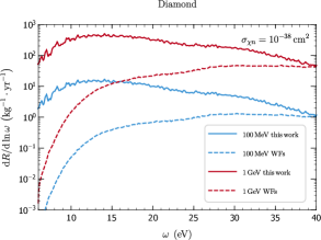
Figure 4: A comparison between the Migdal excitation event rates calculated in this work (in solid) and obtained in Ref. [42] with the localized WFs (in dashed) in crystal diamond, where the red lines represent the event rates of a $1\,\mathrm{GeV}$ DM, and the blues represent the rates of a $100\,\mathrm{MeV}$ DM particle, for the benchmark cross section $\sigma_{\chi n}=10^{-38}\,\mathrm{cm}^{2}$. See text for details.

IV Summary and conclusions

In this paper we make an alternative attempt to describe the Migdal effect in semiconductor targets, in which the description of the Migdal effect separates into two parts. Firstly, we incorporate the bremsstrahlung-like process to account for the drag force exerted on the electrons by the suddenly struck ion, where the Coulomb interaction is mediated by the bremsstrahlung photons. Secondly, many-body effects such as screening, collective behavior are also taken into consideration in the calculation of excitation rate of the electron-hole pairs. Based on this method, the Migdal excitation event rates for diamond and silicon semiconductors are calculated.

As mentioned in previous section, the spectra are modulated by the factor $\omega^{-4}$, which results in a significant boost to the excitation event rate in the low energy regime and a suppression towards the high energy end. Such phenomenon is especially remarkable for a target possessing a small band gap, such as silicon presented in right panel of Fig. 3. It is interesting to make a comparison between the event rates calculated in this work and the ones obtained with the localized WFs in Ref. [42]. For this purpose we present the two spectra for diamond crystal in Fig. 4. Compared to the spectra calculated with the localized WFs in Ref. [42] (in dashed), the event rates calculated in this study (in solid) are found to be significantly larger in the low energy range near the band gap, and turn moderately higher towards the high energy end. Apparently, the $\omega^{-4}$ scaling behavior has not been reflected in the crystal form factor $\mathcal{F}\left(q,\,E_{e}\right)$ calculated in Ref. [42].

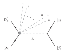
Figure 5: The diagram for the multiphonon process where the DM particle excites an electron-hole pair via the exchange of a single phonon, while most of the transferred momentum of the DM particle is taken by a bunch of $n$ phonons. See text for details.

Finally, we try to interpret this method in the context of the quantization of the crystal vibration. We begin with the diagram in Fig. 5 that represents a process where a pair of electron and hole is excited via the exchange of single phonon, along with a bunch of phonons created by the scattering of the DM particle and nucleus. It is noted that the phonon propagator can be approximated as $iD_{\mathbf{k},\alpha}=i/\left(\varepsilon_{ij}^{2}-\omega_{\mathbf{k},\alpha}^{2}\right)\simeq i/\varepsilon_{ij}^{2}$, because the phonon eigenfrequncy of branch $\alpha$ at transferred momentum $\mathbf{k}$, $\omega_{\mathbf{k},\alpha}\sim\mathcal{O}\left(10^{-1}\mathrm{eV}\right)$, is much smaller than the band gap. As a result of this approximation, the sum over the products of the two vertices relevant for the excitation can be contracted as the following,

$$-\sum_{\alpha}\left(\frac{\boldsymbol{\epsilon}_{\mathbf{k},\alpha}\cdot\mathbf{q}}{\sqrt{m_{N}}}\right)\left(\frac{\boldsymbol{\epsilon}_{\mathbf{k},\alpha}\cdot\mathbf{k}}{\sqrt{m_{N}}}\right) \simeq \frac{\mathbf{p}_{N}\cdot\mathbf{k}}{m_{N}},$$ (19)

where $\boldsymbol{\epsilon}_{\mathbf{k},\alpha}$ is the phonon eigenvector of momentum $\mathbf{k}$. Taking into consideration also the interactions $V_{\chi N}$ and $V_{Ne}$ from the two vertices, respectively, as well as other necessary factors, one observes that the processes in Fig. 1 and Fig. 5 are equivalent, except for a difference in interpreting the recoil effects in the crystal: in Fig. 1 the final state is the recoiled nucleus, whereas in Fig. 5 the final states are a large number of $n$ phonons. In fact, it is implied through an isotropic harmonic oscillator toy model that in the limit $q\rightarrow\infty$, the effects of the multiphonon final states can be well summarized with a recoiled nucleus, which is namely the impulse approximation [59]. In this regard, the two descriptions are essentially identical: the bremsstrahlung-like process in the soft limit is equivalent to a multiphonon process in the impulse approximation, where a valence electron is excited across the band gap via the exchange of a single phonon.

However, in the low momentum transfer regime (or equivalently, in the low DM mass regime), the impulse approximation may no longer be valid, and the recoiling effect should be accounted for with a multiphonon process. A detailed analysis in Ref. [51] indicates that for $m_{\chi}\leq 50\,\mathrm{MeV}$ the impulse approximation ceases to be reliable for silicon and germanium targets, where phonons, rather than a free nucleus, are more appropriate for the description of the recoiling effect.

Note added In the final phase of preparing this paper, which was enlightened by Ref. [50], Ref. [51] appeared, which calculated the Migdal effect in semiconductor targets silicon and germanium with the similar techniques, and provided heuristic explanation for the treatment of the bremsstrahlung-like process, while in this work we calculate the event rates for diamond and silicon. Ref. [51] also pointed out the importance of the contribution of the off-diagonal terms of the dielectric matrix to the total Migdal event rate, which motivates us to further take into account the off-diagonal terms for a complete calculation of the Migdal event rates in diamond and silicon targets.

Appendix A Excitation event rate in the quantum field theory

In this Appendix, we provide some detailed derivation of the formulas in the main text.

A.1 Feynman rules

In order to describe the scattering processes in solids it is necessary to derive the Feynman rules at zero and finite temperatures. Here a brief review is arranged. We begin with the propagators in the position space.

• The DM-nucleus propagator between space-time coordinates $x$ and $x^{\prime}$ is

  $$iS_{\chi N}\left(x,\,x^{\prime}\right) = \sum_{\mathbf{q}}\int iV_{\chi N}\left(\mathbf{q}\right)\frac{e^{i\mathbf{q}\cdot\left(\mathbf{x}-\mathbf{x}^{\prime}\right)}}{V}\frac{e^{-i\omega\left(t_{x}-t_{x^{\prime}}\right)}\mathrm{d}\omega}{2\pi}$$ (20)

  $$= \sum_{\mathbf{q}}\int iV_{\chi N}\left(\mathbf{q}\right)\frac{e^{i\mathbf{q}\cdot\left(\mathbf{x}-\mathbf{x}^{\prime}\right)}}{V}\times\delta\left(t_{x}-t_{x^{\prime}}\right),$$

  in which one neglects the retardation of the interaction in the non-relativistic limit.

• The nucleus propagator between $x$ and $x^{\prime}$ is

  $$iS_{NN}\left(x,\,x^{\prime}\right) = \sum_{\mathbf{\mathbf{p}}}\int\left(\frac{i}{\omega-\varepsilon_{\mathbf{\mathbf{p}}}+i0^{+}}\right)\frac{e^{i\mathbf{\mathbf{p}}\cdot\left(\mathbf{x}-\mathbf{x}^{\prime}\right)}}{V}\frac{e^{-i\omega\left(t_{x}-t_{x^{\prime}}\right)}\mathrm{d}\omega}{2\pi},$$ (21)

  with $\varepsilon_{\mathbf{p}}=\left|\mathbf{p}\right|^{2}/\left(2\,m_{N}\right)$.

• The ion-electron Coulomb potential propagator between $x$ and $x^{\prime}$ is

  $$iD_{\mathrm{Cou}}\left(x,\,x^{\prime}\right) = \sum_{\mathbf{k}}\int iV_{Ne}\left(\mathbf{k}\right)\frac{e^{i\mathbf{k}\cdot\left(\mathbf{x}-\mathbf{x}^{\prime}\right)}}{V}\frac{e^{-i\omega\left(t_{x}-t_{x^{\prime}}\right)}\mathrm{d}\omega}{2\pi}$$ (22)

  $$= \sum_{\mathbf{k}}i\left(\frac{Z_{\mathrm{ion}}4\pi\alpha}{\left|\mathbf{k}\right|^{2}+i0^{+}}\right)\frac{e^{i\mathbf{k}\cdot\left(\mathbf{x}-\mathbf{x}^{\prime}\right)}}{V}\delta\left(t_{x}-t_{x^{\prime}}\right).$$

In addition, the propagator of electrons in the crystal is similar to that of the nucleus. It is not shown here because it does not appear in the Migdal scattering process at the tree level.

On the other hand, we summarize the Feynman rules for the external legs as the following.

• The incoming and outgoing states of the DM particle at space-time coordinate $x$ are represented with $e^{i\mathbf{p}_{\chi}\cdot\mathbf{x}-i\varepsilon_{\mathbf{p}_{\chi}}t_{x}}/\sqrt{V}$ and $e^{-i\mathbf{p}_{\chi}^{\prime}\cdot\mathbf{x}+i\varepsilon_{\mathbf{p}_{\chi}^{\prime}}t_{x}^{\prime}}/\sqrt{V}$, respectively, with their corresponding energies $\varepsilon_{\mathbf{p}_{\chi}}=\left|\mathbf{p}_{\chi}\right|^{2}/\left(2\,m_{\chi}\right)$ and $\varepsilon_{\mathbf{p}_{\chi}^{\prime}}=\left|\mathbf{p}_{\chi}^{\prime}\right|^{2}/\left(2\,m_{\chi}\right)$.

• The incoming and outgoing states of nucleus at $x$ are represented with $e^{i\mathbf{p}_{N}\cdot\mathbf{x}-i\varepsilon_{\mathbf{p}_{N}}t_{x}}/\sqrt{V}$ and $e^{-i\mathbf{p}_{N}^{\prime}\cdot\mathbf{x}+i\varepsilon_{\mathbf{p}_{N}^{\prime}}t_{x}^{\prime}}/\sqrt{V}$, respectively, with their corresponding energies $\varepsilon_{\mathbf{p}_{N}}=\left|\mathbf{p}_{N}\right|^{2}/\left(2\,m_{N}\right)$ and $\varepsilon_{\mathbf{p}_{N}^{\prime}}=\left|\mathbf{p}_{N}^{\prime}\right|^{2}/\left(2\,m_{N}\right)$.

• The incoming and outgoing states of electron in crystal at $x$ are represented with $\psi_{j}\left(\mathbf{x}\right)e^{-i\varepsilon_{j}t_{x}}$ and $\psi_{i}^{*}\left(\mathbf{x}\right)e^{i\varepsilon_{i}t_{x}}$, respectively, with their corresponding energies $\varepsilon_{j}$ and $\varepsilon_{i}$.

It is straightforward to translate above Feynman rules in the position space into those in the momentum space after integrating out the position 4-vector coordinates at each vertex. They are summarized as follows.

• Except for the case concerning the external legs of electrons in solids, each vertex contributes a factor $\left(2\pi\right)V$ and an energy-momentum conservation condition presented as discrete delta functions $\delta_{\left(\sum_{i}\mathbf{p}_{i}\right),\mathbf{0}}\,\delta\left(\sum\varepsilon_{i}\right)$.

• Vertex that contains both the incoming and outgoing states ($\ket{j}$ and $\ket{i}$) of the electrons in solids contributes a factor $\left(2\pi\right)\braket{i}{e^{i\mathbf{p}\cdot\hat{\mathbf{x}}}}{j}$ and the energy conservation condition $\delta\left(\sum\varepsilon_{i}\right)$, where $\mathbf{p}$ is the net momentum that sinks into the vertex.

• Each DM particle or each nucleus external leg contributes a factor $1/\sqrt{V}$.

• Each internal line corresponds to the propagator of its kind, as well as a factor $1/V$. For example, the nucleus internal line is read as $i/\left(\omega-\varepsilon_{\mathbf{\mathbf{p}}}+i0^{+}\right)$ multiplied by a factor $1/V$.

Applying these rules, and summing up all the discrete momenta at each vertex, the $T$-matrix can be expressed in terms of the amplitude as the following,

$$i\mathcal{T} = i\mathcal{M}\,\frac{\left(2\pi\right)}{V}\delta_{\left(\sum_{i}\mathbf{p}_{i}\right),\mathbf{0}}\,\delta\left(\sum\varepsilon_{i}\right).$$ (23)

Above usage of Feynman diagrams and rules in scattering theory can be transplanted to discussions in the linear response theory in a parallel fashion, where the imaginary time $t\rightarrow-i\tau$ is introduced to account for the statistical field theory at a finite temperature. For example, a fermion propagator in the position space is written as

$$S\left(x,\,x^{\prime}\right) = \sum_{i}\sum_{n}\int\frac{u_{i}\left(\mathbf{x}\right)u_{i}^{*}\left(\mathbf{x}^{\prime}\right)}{i\omega_{n}-\varepsilon_{i}}\frac{e^{-i\omega_{n}\left(\tau-\tau^{\prime}\right)}}{\beta},$$ (24)

where $\tau$ and $\tau^{\prime}$ are the “temporal” coordinates, $\beta=1/kT$ is the inverse temperature, with Boltzmann constant $k$, $\omega_{n}=\left(n+\frac{1}{2}\right)\left(2\pi/\beta\right)$ is the Matsubara fermion frequency, with $n$ being an integer to ensure the anti-periodicity, and $u_{i}\left(\mathbf{x}\right)$ is the normalized $i$th eigen wavefunction, with its eigen energy $\varepsilon_{i}$, which can be free or bound state. Base on these propagators, Feynman rules for finite temperature filed theory can also be summarized and applied to calculation of physical quantities such as dielectric functions, and polarizabilities in the context of linear response theory.

A.2 Dielectric function and random phase approximation (RPA)

A.2.1 dielectric function and polarizability

In a system where there is an external electromagnetic perturbation $\phi_{\mathrm{ext}}$, the charge is redistributed and gets polarized. In order to describe the resulting total potential $\phi_{\mathrm{tot}}$ we invoke the inverse dielectric function $\epsilon^{-1}$ in the following way [60],

$$\phi_{\mathrm{tot}}\left(\mathbf{x},t\right) = \int\mathrm{d}^{4}x^{\prime}\,\epsilon^{-1}\left(\mathbf{x},t;\mathbf{x}^{\prime},t^{\prime}\right)\,\phi_{\mathrm{ext}}\left(\mathbf{x}^{\prime},t^{\prime}\right),$$ (25)

$$= \int\mathrm{d}^{4}x^{\prime}\,\left[\delta^{4}\left(x-x^{\prime}\right)+\int\mathrm{d}^{4}x^{\prime\prime}\,V^{\mathrm{Cou}}\left(x,\,x^{\prime\prime}\right)\chi_{\rho\rho}^{\mathrm{r}}\left(\mathbf{x}^{\prime\prime},t^{\prime\prime};\mathbf{x}^{\prime},t^{\prime}\right)\right]\,\phi_{\mathrm{ext}}\left(\mathbf{x}^{\prime},t^{\prime}\right)$$

where $V^{\mathrm{Cou}}\left(x,\,x^{\prime\prime}\right)$ is the instantaneous Coulomb interaction, and the polarizability $\chi_{\rho\rho}^{\mathrm{r}}$ is the density-density correlation function

$$\chi_{\rho\rho}^{\mathrm{r}}\left(\mathbf{x},t;\mathbf{x}^{\prime},t^{\prime}\right) = \left(-i\right)\varTheta\left(t-t^{\prime}\right)\,\left\langle\,\left[\hat{\rho}_{I}\left(\mathbf{x},t\right),\,\hat{\rho}_{I}\left(\mathbf{x}^{\prime},t^{\prime}\right)\right]\,\right\rangle$$ (26)

in the context of linear response theory, with $\left\langle\cdots\right\rangle$ denoting the thermal equilibrium average. In a system with translation-invariance, the polarizability only depends on the differences of the space-time coordinates, i.e., $\chi^{\mathrm{r}}\left(\mathbf{x},t;\mathbf{x}^{\prime},t^{\prime}\right)=\chi^{\mathrm{r}}\left(\mathbf{x}-\mathbf{x}^{\prime},t-t^{\prime};0,0\right)$, so it is convenient to discuss relevant problems in the momentum-energy space, where the inverse dielectric function can be expressed as a product

$$\epsilon^{-1}\left(\mathbf{q},\omega\right) = 1+V^{\mathrm{Cou}}\left(\mathbf{q}\right)\chi_{\rho\rho}^{\mathrm{r}}\left(\mathbf{q},\omega\right),$$ (27)

with $V^{\mathrm{Cou}}\left(\mathbf{q}\right)$ being the reciprocal counterpart of the Coulomb potential in momentum space. Therefore, the calculation of the polarizability plays the central role in our investigation of the response of the solids induced by electromagnetic perturbation, and the DM particle. While the momentum component of $\chi_{\rho\rho}^{\mathrm{r}}\left(\mathbf{q},\omega\right)$ can be obtained by a direct Fourier transformation of Eq. (26), deriving the frequency part at a finite temperature needs to be carried out with imaginary time Green’s functions, or the so-called Matsubara Green’s functions. The procedure for the density-density correlation is briefly summarized as follows. First, one introduces the Matsubara Green’s function, which is defined as

$$\chi_{\rho\rho}\left(\mathbf{q},\tau\right) = -\int_{V}\left\langle\,\hat{T}_{\tau}\left[\hat{\rho}_{I}\left(\mathbf{x},\tau\right),\,\hat{\rho}_{I}\left(\mathbf{0},0\right)\right]\,\right\rangle e^{-i\mathbf{q}\cdot\mathbf{x}}\,\mathrm{d}^{3}x$$ (28)

$$= \sum_{n}\chi_{\rho\rho}\left(\mathbf{q},i\nu_{n}\right)\frac{e^{-i\nu_{n}\tau}}{\beta},$$

where $\hat{T}_{\tau}$ is the imaginary time-ordering operator, $\beta>\tau>0$, and $\nu_{n}=n\left(2\pi/\beta\right)$ is bosonic frequency since $\hat{\rho}$ is a bosonic operator, with $n$ being an integer to ensure the periodicity. Then one obtains $\chi_{\rho\rho}^{\mathrm{r}}\left(i\nu_{n}\right)$ with the Fourier transformation

$$\chi_{\rho\rho}\left(\mathbf{q},i\nu_{n}\right) = \int_{0}^{\beta}\chi_{\rho\rho}\left(\mathbf{q},\tau\right)\,e^{i\nu_{n}\tau}\mathrm{d}\tau.$$ (29)

With the Lehmann representation, it is observed that $\chi_{\rho\rho}^{\mathrm{r}}\left(\mathbf{q},\omega\right)$ and $\chi_{\rho\rho}\left(\mathbf{q},i\nu_{n}\right)$ are just special case of the same function defined in the entire complex plane except for a series of poles lying along the real axis. Thus, once $\chi_{\rho\rho}\left(\mathbf{q},i\nu_{n}\right)$ is obtained from Eq. (29), the retarded polarizability can be derived by performing the analytic continuation $\chi_{\rho\rho}^{\mathrm{r}}\left(\mathbf{q},\omega\right)=\chi_{\rho\rho}\left(\mathbf{q},i\nu_{n}\rightarrow\omega+i0^{+}\right)$.

A.2.2 RPA

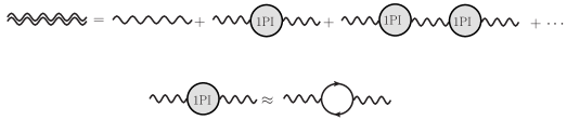
Figure 6: Top: The diagrammatic expansion of the Schwinger-Dyson equation for the screened Coulomb interaction, where the double wiggle line on the left-hand-side of equation represents the renormalized Coulomb interaction, while the single wiggle represents a bare Coulomb interaction. Bottom: In the RPA, 1PI diagram is approximated as an electron-hole loop. See text for details.

The linear response theory can be discussed with our familiar language of path integrals, as well as necessary modifications accounting for the imaginary-time argument. The dielectric properties can be described in terms of diagrams in the top panel of Fig. 6, where the Schwinger-Dyson equation for the screened Coulomb interaction is represented by a bare interaction wiggly line attached to a geometric series over polarization bubbles. If we use $W$ and $\Pi$ to represent the screened Coulomb potential, and the self-energy corresponding to the 1-particle-irreducible (1PI) blob, respectively, the infinite sum is read as

$$W = \frac{V^{\mathrm{Cou}}}{\epsilon}$$ (30)

$$= V^{\mathrm{Cou}}+V^{\mathrm{Cou}}\left[\Pi+\Pi\,V^{\mathrm{Cou}}\,\Pi+\Pi\,V^{\mathrm{Cou}}\,\Pi\,V^{\mathrm{Cou}}\,\Pi+\cdots\right]V^{\mathrm{Cou}}$$

$$= \frac{V^{\mathrm{Cou}}}{1-V^{\mathrm{Cou}}\,\Pi},$$

and hence one has

$$\epsilon\left(\mathbf{q},i\nu_{n}\right) = 1-V^{\mathrm{Cou}}\left(\mathbf{q}\right)\,\Pi\left(\mathbf{q},i\nu_{n}\right).$$ (31)

On the other hand, adopting the random phase approximation (RPA) means that, only the electron-hole bubble is retained among all 1PI diagrams in calculation of the dielectric functions, which is illustrated in the bottom panel of Fig. 6. Thus within the framework of RPA, starting from Eq. (28) and Eq. (29), one first obtains the 1PI blob

$$\Pi\left(\mathbf{q},i\nu_{n}\right) \simeq \frac{1}{V}\sum_{i,j}\frac{\left|\braket{i}{e^{i\mathbf{q}\cdot\hat{\mathbf{x}}}}{j}\right|^{2}}{\varepsilon_{ij}-i\nu_{n}}\left(n_{i}-n_{j}\right),$$ (32)

where $n_{i}$ ($n_{j}$) denotes the occupation number of the state $\ket{i}$ ($\ket{j}$), and then performing the analytic extension $i\nu_{n}\rightarrow\omega+i0^{+}$ and inserting the polarizability into Eq. (27), one finally arrives at the Lindhard dielectric function

$$\epsilon^{\mathrm{RPA}}\left(\mathbf{q},\omega\right) = 1-\frac{V^{\mathrm{Cou}}\left(\mathbf{q}\right)}{V}\sum_{i,j}\frac{\left|\braket{i}{e^{i\mathbf{q}\cdot\hat{\mathbf{x}}}}{j}\right|^{2}}{\varepsilon_{ij}-\omega-i0^{+}}\left(n_{i}-n_{j}\right)$$ (33)

and its inverse

$$\mathrm{Im}\left[\frac{-1}{\epsilon^{\mathrm{RPA}}\left(\mathbf{q},\omega\right)}\right] \simeq \mathrm{Im}\left[-1-\frac{V^{\mathrm{Cou}}\left(\mathbf{q}\right)}{V}\sum_{i,j}\frac{\left|\braket{i}{e^{i\mathbf{q}\cdot\hat{\mathbf{x}}}}{j}\right|^{2}}{\varepsilon_{ij}-\omega-i0^{+}}\left(n_{i}-n_{j}\right)\right]$$ (34)

$$= 2\pi\frac{V^{\mathrm{Cou}}\left(\mathbf{q}\right)}{V}\,\sum_{i,\,j}\left|\braket{i}{e^{i\mathbf{q}\cdot\hat{\mathbf{x}}}}{j}\right|^{2}\,\delta\left(\varepsilon_{i}-\varepsilon_{j}-\omega\right).$$

In above discussion we assume that the electronic system possesses a translational symmetry, which is true for the case such as homogeneous electron gas (HEG). However, for the case of crystal structure where the translational symmetry for continuous space reduces to that for the crystal lattice, the polarizability can no longer be expressed as differences of the space-time coordinates. In this case, the double periodic position function such as $\chi\left(\mathbf{x},\mathbf{x}^{\prime};\omega\right)$ can be expressed in the reciprocal space as the following,

$$\chi\left(\mathbf{x},\mathbf{x}^{\prime};\omega\right) = \frac{1}{V}\sum_{\mathbf{q}\in 1\mathrm{BZ}}\sum_{\mathbf{G},\mathbf{G}^{\prime}}e^{i\left(\mathbf{q}+\mathbf{G}\right)\cdot\mathbf{x}}\,\chi_{\mathbf{G},\mathbf{G}^{\prime}}\left(\mathbf{q};\omega\right)\,e^{-i\left(\mathbf{q}+\mathbf{G}^{\prime}\right)\cdot\mathbf{x}^{\prime}}$$ (35)

where $\chi_{\mathbf{G},\mathbf{G}^{\prime}}\left(\mathbf{q};\omega\right)$ is the reciprocal matrix with $\mathbf{G}$ and $\mathbf{G}^{\prime}$ being reciprocal lattice vectors and $\mathbf{q}$ is restricted to the first BZ, which can be determined with the Fourier transformation

$$\chi_{\mathbf{G},\mathbf{G}^{\prime}}\left(\mathbf{q};\omega\right) = \frac{1}{V}\int\mathrm{d}^{3}x\,\mathrm{d}^{3}x\,^{\prime}e^{-i\left(\mathbf{q}+\mathbf{G}\right)\cdot\mathbf{x}}\chi\left(\mathbf{x},\mathbf{x}^{\prime};\omega\right)\,e^{i\left(\mathbf{q}+\mathbf{G}^{\prime}\right)\cdot\mathbf{x}^{\prime}}.$$ (36)

As a consequence, for an arbitrary momentum transfer $\mathbf{Q}$, which can be split into a reduced momentum confined in the 1BZ, and a reciprocal one, i.e., $\mathbf{\mathbf{Q}}=\mathbf{q}+\mathbf{G}$, above Lindhard formula relevant for the excitation is generalized to the following microscopic dielectric matrix:

$$\epsilon_{\mathbf{G},\mathbf{G}^{\prime}}^{\mathrm{RPA}}\left(\mathbf{q},\omega\right) = \delta_{\mathbf{G},\mathbf{G}^{\prime}}-\frac{V_{\mathbf{G},\mathbf{G}}^{\mathrm{Cou}}\left(\mathbf{q}\right)}{V}\sum_{i,j}\frac{\braket{i}{e^{i\left(\mathbf{\mathbf{\mathbf{q}+\mathbf{G}}}^{\prime}\right)\cdot\hat{\mathbf{x}}}}{j}\braket{j}{e^{-i\left(\mathbf{\mathbf{\mathbf{q}+\mathbf{G}}}\right)\cdot\hat{\mathbf{x}}}}{i}}{\varepsilon_{ij}-\omega-i0^{+}}\left(n_{i}-n_{j}\right)$$

$$= \delta_{\mathbf{G},\mathbf{G}^{\prime}}-\frac{2\times 4\pi\alpha}{V\,\left|\mathbf{q}+\mathbf{G}\right|^{2}}\sum_{i^{\prime}}^{c}\sum_{i}^{v}\sum_{\mathbf{k},\mathbf{k}^{\prime}\in 1\mathrm{BZ}}\left[-\frac{\braket{i^{\prime}\,\mathbf{k}^{\prime}}{e^{i\left(\mathbf{\mathbf{\mathbf{q}+\mathbf{G}}}^{\prime}\right)\cdot\hat{\mathbf{x}}}}{i\,\mathbf{k}}\braket{i^{\prime}\,\mathbf{k}^{\prime}}{e^{i\left(\mathbf{\mathbf{\mathbf{q}+\mathbf{G}}}\right)\cdot\hat{\mathbf{x}}}}{i\,\mathbf{k}}^{*}}{\varepsilon_{i^{\prime}\,\mathbf{k}^{\prime}}-\varepsilon_{i\,\mathbf{k}}-\omega-i0^{+}}\right]$$

$$= \delta_{\mathbf{G},\mathbf{G}^{\prime}}+\frac{2\times 4\pi\alpha}{V\,\left|\mathbf{q}+\mathbf{G}\right|^{2}}\sum_{i^{\prime}}^{c}\sum_{i}^{v}\sum_{\mathbf{k}\in 1\mathrm{BZ}}\left[\frac{\left(\int_{\Omega}\mathrm{d}^{3}x\,u_{i^{\prime}\mathbf{k}+\mathbf{q}}^{*}\left(\mathbf{x}\right)\,e^{i\mathbf{\mathbf{G}}^{\prime}\cdot\mathbf{x}}\,u_{i\mathbf{k}}\left(\mathbf{x}\right)\right)\left(\int_{\Omega}\mathrm{d}^{3}x\,u_{i^{\prime}\mathbf{k}+\mathbf{q}}^{*}\left(\mathbf{x}\right)\,e^{i\mathbf{\mathbf{G}}\cdot\mathbf{x}}\,u_{i\mathbf{k}}\left(\mathbf{x}\right)\right)^{*}}{\varepsilon_{i^{\prime}\,\mathbf{k}+\mathbf{q}}-\varepsilon_{i\,\mathbf{k}}-\omega-i0^{+}}\right],$$

where $V_{\mathbf{G},\mathbf{G}^{\prime}}^{\mathrm{Cou}}\left(\mathbf{q}\right)=V^{\mathrm{Cou}}\left(\mathbf{q}+\mathbf{G}\right)\delta_{\mathbf{G},\mathbf{G}^{\prime}}=4\pi\alpha\,\delta_{\mathbf{G},\mathbf{G}^{\prime}}/\left|\mathbf{q}+\mathbf{G}\right|^{2}$ is obtained from Eq. (36), and the inverse dielectric function can be determined via matrix inversion.

A.2.3 Cross section and event rate

Here we first derive a general formula dedicated to the calculation of two-body scattering cross section for the case of discrete momenta. By modifying the derivation in textbook, we obtain the cross section between particles $A$ and $B$,

$$\sigma = \left(\prod_{f}\sum_{\mathbf{p}_{f}}\right)\frac{\left|\mathcal{M}\left(\mathbf{k}_{A},\mathbf{k}_{B}\rightarrow\left\{\mathbf{p}_{f}\right\}\right)\right|^{2}}{\left|\mathbf{v}_{A}-\mathbf{v}_{B}\right|}\frac{\left(2\pi\right)}{V}\,\delta_{\mathbf{k}_{A}+\mathbf{k}_{B},\sum_{{}_{f}}\mathbf{p}_{f}}\,\delta\left(\varepsilon_{A}+\varepsilon_{B}-\sum_{f}\varepsilon_{f}\right),$$ (38)

where $\mathbf{v}_{A}-\mathbf{v}_{B}$ is the relative velocity between the two particles, $\mathbf{p}_{f}$ is the momentum of the $f$th outgoing particle, and $\mathcal{M}\left(\mathbf{k}_{A},\mathbf{k}_{B}\rightarrow\left\{\mathbf{p}_{f}\right\}\right)$ is the amplitude in the discrete momentum space. Following the aforementioned Feynman rules, one can read and approximate the $T$-matrix from Fig. 1 as follows

$$\braket{\mathbf{p}^{\prime}_{\chi}\mathbf{p}_{N}\mathrm{;electron\,hole\,pair}}{iT}{\mathbf{p}_{\chi}\mathbf{0}_{N}} = i\frac{\left(2\pi\right)}{V}\sum_{\mathbf{k}}\delta_{\mathbf{p}^{\prime}_{\chi}+\mathbf{p}_{N}+\mathbf{k},\,\mathbf{p}{}_{\chi}}\delta\left(\sum_{i}\varepsilon_{i}\right)\times\left(\cdots\right)_{\mathbf{k}}$$ (39)

$$\simeq i\frac{\left(2\pi\right)}{V}\delta_{\mathbf{p}^{\prime}_{\chi}+\mathbf{p}_{N},\,\mathbf{p}{}_{\chi}}\delta\left(\sum_{i}\varepsilon_{i}\right)\times\sum_{\mathbf{k}}\left(\cdots\right)_{\mathbf{k}}$$

$$= \frac{\left(2\pi\right)}{V}\delta_{\mathbf{p}^{\prime}_{\chi}+\mathbf{p}_{N},\,\mathbf{p}{}_{\chi}}\delta\left(\sum_{i}\varepsilon_{i}\right)\times i\mathcal{M},$$

where in the first line we separate out four-momentum conservation condition from other terms dependent on transferred momentum $\mathbf{k}$ of the Coulomb potential, and in the second line we assume that $\mathbf{k}$ is much softer than that of the recoiling nucleus $\mathbf{p}_{N}$, which is consistent with the soft limit condition and explains the summation over $\mathbf{k}$ in Eq. (1). Thus, one obtains the total cross section of an incident DM particle exciting an electron across the Fermi surface for the HEG via a recoiling nucleus,

$$\sigma = \sum_{i,\,j}\sum_{\mathbf{k}^{\prime},\mathbf{k}}\sum_{\mathbf{\mathbf{p}^{\prime}_{\chi}}}\sum_{\mathbf{p}_{N}}\frac{2\pi}{V}\int\mathrm{d}\omega\frac{\mathcal{\left|M\right|}^{2}}{v\,\epsilon^{*}\left(\mathbf{k}^{\prime},\omega\right)\epsilon\left(\mathbf{k},\omega\right)}\delta_{\mathbf{p}^{\prime}_{\chi}+\mathbf{p}_{N},\,\mathbf{p}{}_{\chi}}\,\delta\left[\frac{p_{\chi}^{\prime 2}}{2m_{\chi}}-\frac{p_{\chi}^{2}}{2m_{\chi}}+\frac{p_{N}^{2}}{2m_{N}}+\varepsilon_{ij}\right]\delta\left(\varepsilon_{ij}-\omega\right)$$ (40)

$$= \sum_{\mathbf{k}}\sum_{\mathbf{p}_{N}}\left(\frac{2\pi}{V}\right)\left(\frac{A^{2}\pi\sigma_{\chi n}}{\pi\mu_{\chi n}^{2}\,v}\right)\left(\frac{4\pi\,Z_{\mathrm{ion}}^{2}\,\alpha}{V\,}\right)\int\frac{\mathrm{d}\omega}{\omega^{4}}\,\frac{\left|\mathbf{p}_{N}\cdot\mathbf{\hat{k}}\right|^{2}}{m_{N}^{2}}\,\delta\left[\frac{p_{N}^{2}}{2\mu_{\chi N}}-\mathbf{v}\cdot\mathbf{p}_{N}+\omega\right]$$

$$\times\frac{1}{\left|\epsilon\left(\mathbf{k},\omega\right)\right|^{2}}\sum_{i,\,j}\frac{2\times 4\pi^{2}\alpha}{V\,k^{2}}\left|\braket{i}{e^{i\mathbf{k}\cdot\hat{\mathbf{x}}}}{j}\right|^{2}\delta\left(\varepsilon_{ij}-\omega\right)$$

$$= \frac{8\pi^{2}A^{2}\sigma_{\chi n}\,Z_{\mathrm{ion}}^{2}\,\alpha}{\mu_{\chi n}^{2}\,v\,}\int\frac{\mathrm{d}^{3}p_{N}}{\left(2\pi\right)^{3}}\int\frac{\mathrm{d}\omega}{\omega^{4}}\,\,\delta\left[\frac{p_{N}^{2}}{2\mu_{\chi N}}-\mathbf{v}\cdot\mathbf{p}_{N}+\omega\right]\int\frac{\mathrm{d}^{3}k}{\left(2\pi\right)^{3}}\frac{\left|\mathbf{p}_{N}\cdot\mathbf{\hat{k}}\right|^{2}}{m_{N}^{2}}\,\mathrm{Im}\left[\frac{-1}{\epsilon\left(\mathbf{k},\omega\right)}\right]$$

$$= \frac{8\pi^{2}A^{2}\sigma_{\chi n}\,Z_{\mathrm{ion}}^{2}\,\alpha}{3\,\mu_{\chi n}^{2}\,v\,\left(2\pi\right)^{6}}\int\left|\mathbf{v}_{\mathrm{ion}}\right|^{2}\,\mathrm{d}^{3}p_{N}\int\frac{\mathrm{d}\omega}{\omega^{4}}\,\,\delta\left[\frac{p_{N}^{2}}{2\mu_{\chi N}}-\mathbf{v}\cdot\mathbf{p}_{N}+\omega\right]\int\mathrm{d}^{3}k\,\mathrm{Im}\left[\frac{-1}{\epsilon\left(\mathbf{k},\omega\right)}\right],$$

where $v$ is the velocity of the DM particle in the frame of laboratory, $\mathbf{v}_{\mathrm{ion}}=\mathbf{p}_{N}/m_{N}$ is the velocity of the recoiled nucleus, and $-\mathrm{Im}\left[\epsilon^{-1}\left(\mathbf{k},\omega\right)\right]$ is called the loss function. Since the amplitude $\braket{i}{e^{i\mathbf{k}\cdot\hat{\mathbf{x}}}}{j}$ uniquely pins down the momentum $\mathbf{k}$ (through the momentum conservation), only the diagonal terms of momenta $\mathbf{k}$’s are relevant in above calculation for the HEG. Following Refs. [49, 50], we adopt a Coulomb potential between the recoiled ion and electrons screened by dielectric function $\epsilon\left(\mathbf{k},\omega\right)$ so as to obtain a general formula that includes self-interaction effects of the Coulomb propagator. To this end, we take the correspondence

$$2\times\sum_{i,\,j}\frac{4\pi^{2}\alpha}{V\,k^{2}}\left|\braket{i}{e^{i\mathbf{k}\cdot\hat{\mathbf{x}}}}{j}\right|^{2}\delta\left(\varepsilon_{ij}-\omega\right) \rightarrow \mathrm{Im}\left[\epsilon\left(\mathbf{k},\omega\right)\right],$$ (41)

and use the relation

$$\frac{\mathrm{Im}\left[\epsilon\left(\mathbf{k},\omega\right)\right]}{\left|\epsilon\left(\mathbf{k},\omega\right)\right|^{2}} = \mathrm{Im}\left[\frac{-1}{\epsilon\left(\mathbf{k},\omega\right)}\right].$$ (42)

Thus, from Eq. (40) one gives the Migdal exciting event rate

$$R = \frac{\rho_{\chi}}{m_{\chi}}N_{T}\left\langle\sigma v\right\rangle$$ (43)

$$= \frac{\rho_{\chi}}{m_{\chi}}\frac{8\pi^{2}A^{2}\sigma_{\chi n}\,Z_{\mathrm{ion}}^{2}\,\alpha\,N_{T}}{3\,\mu_{\chi n}^{2}\,\left(2\pi\right)^{6}}\int\mathrm{d^{3}}v\,f_{\chi}\left(\mathbf{v}\right)\int\left|\mathbf{v}_{\mathrm{ion}}\right|^{2}\,\mathrm{d}^{3}p_{N}\int\frac{\mathrm{d}\omega}{\omega^{4}}\,\,\delta\left[\frac{p_{N}^{2}}{2\mu_{\chi N}}-\mathbf{v}\cdot\mathbf{p}_{N}+\omega\right]\int\mathrm{d}^{3}k\,\mathrm{Im}\left[\frac{-1}{\epsilon\left(\mathbf{k},\omega\right)}\right]$$

$$= \frac{\rho_{\chi}}{m_{\chi}}\frac{2A^{2}\sigma_{\chi n}\,Z_{\mathrm{ion}}^{2}\,\alpha\,N_{T}}{3\,\mu_{\chi n}^{2}\,\varOmega\,m_{N}^{2}}\int\mathrm{d^{3}}v\,\frac{f_{\chi}\left(\mathbf{v}\right)}{v}\,\int p{}_{N}^{3}\,\mathrm{d}p_{N}\int\frac{\mathrm{d}\omega}{\omega^{4}}\,\varTheta\left[v-v_{\mathrm{min}}\left(p_{N},\,\omega\right)\right]\int\frac{\varOmega\,\mathrm{d}^{3}k}{\left(2\pi\right)^{3}}\,\mathrm{Im}\left[\frac{-1}{\epsilon\left(\mathbf{k},\omega\right)}\right],$$

where $v_{\mathrm{min}}$ is defined in Eq. (8). In contrast to the case in HEG, in crystalline environment both the diagonal and the off-diagonal terms contribute to the total event rate , because in this case $\braket{i}{e^{i\mathbf{k}\cdot\hat{\mathbf{x}}}}{j}$ only constrains momentum $\mathbf{k}$ up to a reciprocal lattice vector $\mathbf{G}$, and thus the off-diagonal terms $\left(\mathbf{G},\,\mathbf{G}^{\prime}\right)$ survive when generalizing the above formula:

$$R = \frac{\rho_{\chi}}{m_{\chi}}\frac{\pi A^{2}\sigma_{\chi n}\,Z_{\mathrm{ion}}^{2}\,N_{T}}{\mu_{\chi n}^{2}\,\left(2\pi\right)^{3}}\int\mathrm{d^{3}}v\,\frac{f_{\chi}\left(\mathbf{v}\right)}{v}\int\,\frac{\mathrm{d}^{3}p_{N}}{p_{N}}\int\frac{\mathrm{d}\omega}{\omega^{4}}\,\varTheta\left[v-v_{\mathrm{min}}\left(p_{N},\,\omega\right)\right]$$ (44)

$$\times\sum_{\mathbf{G}^{\prime},\mathbf{G}}\int_{1\mathrm{BZ}}\frac{\mathrm{d}^{3}\left[k\right]}{\left(2\pi\right)^{3}}\,\left[\frac{\mathbf{p}_{N}\cdot\left(\left[\mathbf{k}\right]+\mathbf{G}\right)}{m_{N}}\right]\left[\frac{\mathbf{p}_{N}\cdot\left(\left[\mathbf{k}\right]+\mathbf{G}^{\prime}\right)}{m_{N}}\right]\mathrm{Im}\left[-\epsilon_{\mathbf{G},\mathbf{G}^{\prime}}^{-1\mathrm{\left(RPA\right)}}\left(\mathbf{\left[\mathbf{k}\right]},\omega\right)\right]V_{\mathbf{G}^{\prime},\mathbf{G}^{\prime}}^{\mathrm{Cou}}\left(\mathbf{\left[\mathbf{k}\right]}\right),$$

where $\epsilon^{-1\mathrm{\left(RPA\right)}}$ is the inverse dielectric matrix introduced in Eq. (LABEL:eq:RPA_matrix). Using the Legendre addition theorem, one first integrates out the solid angle of nucleus momentum $\mathbf{p}_{N}$, and then the event rate is recast as

$$R = \frac{\rho_{\chi}}{m_{\chi}}\frac{2A^{2}\sigma_{\chi n}\,Z_{\mathrm{ion}}^{2}\,\alpha\,N_{T}}{3\,\mu_{\chi n}^{2}\,\varOmega\,m_{N}^{2}}\int\mathrm{d^{3}}v\,\frac{f_{\chi}\left(\mathbf{v}\right)}{v}\int p{}_{N}^{3}\,\mathrm{d}p_{N}\int\frac{\mathrm{d}\omega}{\omega^{4}}\,\varTheta\left[v-v_{\mathrm{min}}\left(p_{N},\,\omega\right)\right]$$ (45)

$$\times\sum_{\mathbf{G},\mathbf{G}^{\prime}}\int_{1\mathrm{BZ}}\frac{\varOmega\,\mathrm{d}^{3}\left[k\right]}{\left(2\pi\right)^{3}}\,\frac{\left(\left[\mathbf{k}\right]+\mathbf{G}\right)\cdot\left(\left[\mathbf{k}\right]+\mathbf{G}^{\prime}\right)}{\left|\left[\mathbf{k}\right]+\mathbf{G}^{\prime}\right|^{2}}\,\mathrm{Im}\left[-\epsilon_{\mathbf{G},\mathbf{G}^{\prime}}^{-1\mathrm{\left(RPA\right)}}\left(\mathbf{\left[k\right]},\omega\right)\right].$$

In practical implementation of the $\mathtt{YAMBO}$ code, an alternative dielectric matrix $\widetilde{\epsilon}_{\mathbf{G},\mathbf{G}^{\prime}}^{\mathrm{\left(RPA\right)}}\left(\mathbf{\left[k\right]},\omega\right)=\left|\left[\mathbf{k}\right]+\mathbf{G}\right|\cdot\epsilon_{\mathbf{G},\mathbf{G}^{\prime}}^{\mathrm{\left(RPA\right)}}\left(\mathbf{\left[k\right]},\omega\right)\cdot\left|\left[\mathbf{k}\right]+\mathbf{G}^{\prime}\right|^{-1}$, or equivalently, $\widetilde{\epsilon}_{\mathbf{G},\mathbf{G}^{\prime}}^{-1\mathrm{\left(RPA\right)}}\left(\mathbf{\left[k\right]},\omega\right)=\left|\left[\mathbf{k}\right]+\mathbf{G}\right|\cdot\epsilon_{\mathbf{G},\mathbf{G}^{\prime}}^{-1\mathrm{\left(RPA\right)}}\left(\mathbf{\left[k\right]},\omega\right)\cdot\left|\left[\mathbf{k}\right]+\mathbf{G}^{\prime}\right|^{-1}$ is preferred, so above event rate is expressed in a symmetrized manner as follows,

$$R = \frac{\rho_{\chi}}{m_{\chi}}\frac{2A^{2}\sigma_{\chi n}\,Z_{\mathrm{ion}}^{2}\,\alpha\,N_{T}}{3\,\mu_{\chi n}^{2}\,\varOmega\,m_{N}^{2}}\int\mathrm{d^{3}}v\,\frac{f_{\chi}\left(\mathbf{v}\right)}{v}\int p{}_{N}^{3}\,\mathrm{d}p_{N}\int\frac{\mathrm{d}\omega}{\omega^{4}}\,\varTheta\left[v-v_{\mathrm{min}}\left(p_{N},\,\omega\right)\right]$$ (46)

$$\times\sum_{\mathbf{G},\mathbf{G}^{\prime}}\int_{1\mathrm{BZ}}\frac{\varOmega\,\mathrm{d}^{3}\left[k\right]}{\left(2\pi\right)^{3}}\,\frac{\left(\left[\mathbf{k}\right]+\mathbf{G}\right)\cdot\left(\left[\mathbf{k}\right]+\mathbf{G}^{\prime}\right)}{\left|\left[\mathbf{k}\right]+\mathbf{G}\right|\left|\left[\mathbf{k}\right]+\mathbf{G}^{\prime}\right|}\,\mathrm{Im}\left[-\widetilde{\epsilon}_{\mathbf{G},\mathbf{G}^{\prime}}^{-1\mathrm{\left(RPA\right)}}\left(\mathbf{\left[k\right]},\omega\right)\right].$$

References

- [1] R. Essig, J. Mardon and T. Volansky, Direct Detection of Sub-GeV Dark Matter, Phys. Rev. D85 (2012) 076007 [1108.5383].
- [2] P. W. Graham, D. E. Kaplan, S. Rajendran and M. T. Walters, Semiconductor Probes of Light Dark Matter, Phys. Dark Univ. 1 (2012) 32 [1203.2531].
- [3] R. Essig, M. Fernandez-Serra, J. Mardon, A. Soto, T. Volansky and T.-T. Yu, Direct Detection of sub-GeV Dark Matter with Semiconductor Targets, JHEP 05 (2016) 046 [1509.01598].
- [4] Y. Hochberg, T. Lin and K. M. Zurek, Absorption of light dark matter in semiconductors, Phys. Rev. D95 (2017) 023013 [1608.01994].
- [5] Y. Hochberg, Y. Kahn, M. Lisanti, K. M. Zurek, A. G. Grushin, R. Ilan et al., Detection of sub-MeV Dark Matter with Three-Dimensional Dirac Materials, Phys. Rev. D97 (2018) 015004 [1708.08929].
- [6] A. Coskuner, A. Mitridate, A. Olivares and K. M. Zurek, Directional Dark Matter Detection in Anisotropic Dirac Materials, 1909.09170.
- [7] R. M. Geilhufe, F. Kahlhoefer and M. W. Winkler, Dirac Materials for Sub-MeV Dark Matter Detection: New Targets and Improved Formalism, 1910.02091.
- [8] Y. Hochberg, Y. Zhao and K. M. Zurek, Superconducting Detectors for Superlight Dark Matter, Phys. Rev. Lett. 116 (2016) 011301 [1504.07237].
- [9] Y. Hochberg, T. Lin and K. M. Zurek, Detecting Ultralight Bosonic Dark Matter via Absorption in Superconductors, Phys. Rev. D94 (2016) 015019 [1604.06800].
- [10] S. Knapen, T. Lin and K. M. Zurek, Light Dark Matter in Superfluid Helium: Detection with Multi-excitation Production, Phys. Rev. D95 (2017) 056019 [1611.06228].
- [11] A. Caputo, A. Esposito and A. D. Polosa, Sub-MeV Dark Matter and the Goldstone Modes of Superfluid Helium, 1907.10635.
- [12] A. Caputo, A. Esposito, E. Geoffray, A. D. Polosa and S. Sun, Dark Matter, Dark Photon and Superfluid He-4 from Effective Field Theory, 1911.04511.
- [13] S. Griffin, S. Knapen, T. Lin and K. M. Zurek, Directional Detection of Light Dark Matter with Polar Materials, Phys. Rev. D98 (2018) 115034 [1807.10291].
- [14] S. Knapen, T. Lin, M. Pyle and K. M. Zurek, Detection of Light Dark Matter With Optical Phonons in Polar Materials, Phys. Lett. B785 (2018) 386 [1712.06598].
- [15] B. Campbell-Deem, P. Cox, S. Knapen, T. Lin and T. Melia, Multiphonon excitations from dark matter scattering in crystals, 1911.03482.
- [16] C. Kouvaris and J. Pradler, Probing sub-GeV Dark Matter with conventional detectors, Phys. Rev. Lett. 118 (2017) 031803 [1607.01789].
- [17] N. F. Bell, J. B. Dent, J. L. Newstead, S. Sabharwale and T. J. Weiler, The Migdal Effect and Photon Bremsstrahlung in effective field theories of dark matter direct detection and coherent elastic neutrino-nucleus scattering, 1905.00046.
- [18] R. Essig, A. Manalaysay, J. Mardon, P. Sorensen and T. Volansky, First Direct Detection Limits on sub-GeV Dark Matter from XENON10, Phys. Rev. Lett. 109 (2012) 021301 [1206.2644].
- [19] S. K. Lee, M. Lisanti, S. Mishra-Sharma and B. R. Safdi, Modulation Effects in Dark Matter-Electron Scattering Experiments, Phys. Rev. D92 (2015) 083517 [1508.07361].
- [20] Y. Hochberg, M. Pyle, Y. Zhao and K. M. Zurek, Detecting Superlight Dark Matter with Fermi-Degenerate Materials, JHEP 08 (2016) 057 [1512.04533].
- [21] I. M. Bloch, R. Essig, K. Tobioka, T. Volansky and T.-T. Yu, Searching for Dark Absorption with Direct Detection Experiments, JHEP 06 (2017) 087 [1608.02123].
- [22] S. Derenzo, R. Essig, A. Massari, A. Soto and T.-T. Yu, Direct Detection of sub-GeV Dark Matter with Scintillating Targets, Phys. Rev. D96 (2017) 016026 [1607.01009].
- [23] Y. Hochberg, Y. Kahn, M. Lisanti, C. G. Tully and K. M. Zurek, Directional detection of dark matter with two-dimensional targets, Phys. Lett. B772 (2017) 239 [1606.08849].
- [24] R. Essig, J. Mardon, O. Slone and T. Volansky, Detection of sub-GeV Dark Matter and Solar Neutrinos via Chemical-Bond Breaking, Phys. Rev. D95 (2017) 056011 [1608.02940].
- [25] F. Kadribasic, N. Mirabolfathi, K. Nordlund, A. E. Sand, E. Holmstrom and F. Djurabekova, Directional Sensitivity In Light-Mass Dark Matter Searches With Single-Electron Resolution Ionization Detectors, Phys. Rev. Lett. 120 (2018) 111301 [1703.05371].
- [26] R. Essig, T. Volansky and T.-T. Yu, New Constraints and Prospects for sub-GeV Dark Matter Scattering off Electrons in Xenon, Phys. Rev. D96 (2017) 043017 [1703.00910].
- [27] A. Arvanitaki, S. Dimopoulos and K. Van Tilburg, Resonant absorption of bosonic dark matter in molecules, Phys. Rev. X8 (2018) 041001 [1709.05354].
- [28] R. Budnik, O. Chesnovsky, O. Slone and T. Volansky, Direct Detection of Light Dark Matter and Solar Neutrinos via Color Center Production in Crystals, Phys. Lett. B782 (2018) 242 [1705.03016].
- [29] P. Sharma, Role of nuclear charge change and nuclear recoil on shaking processes and their possible implication on physical processes, Nuclear Physics A 968 (2017) 326 .
- [30] G. Cavoto, F. Luchetta and A. D. Polosa, Sub-GeV Dark Matter Detection with Electron Recoils in Carbon Nanotubes, Phys. Lett. B776 (2018) 338 [1706.02487].
- [31] Z.-L. Liang, L. Zhang, P. Zhang and F. Zheng, The wavefunction reconstruction effects in calculation of DM-induced electronic transition in semiconductor targets, JHEP 01 (2019) 149 [1810.13394].
- [32] M. Heikinheimo, K. Nordlund, K. Tuominen and N. Mirabolfathi, Velocity Dependent Dark Matter Interactions in Single-Electron Resolution Semiconductor Detectors with Directional Sensitivity, Phys. Rev. D99 (2019) 103018 [1903.08654].
- [33] T. Trickle, Z. Zhang, K. M. Zurek, K. Inzani and S. Griffin, Multi-Channel Direct Detection of Light Dark Matter: Theoretical Framework, 1910.08092.
- [34] T. Trickle, Z. Zhang and K. M. Zurek, Direct Detection of Light Dark Matter with Magnons, 1905.13744.
- [35] R. Catena, T. Emken, N. Spaldin and W. Tarantino, Atomic responses to general dark matter-electron interactions, 1912.08204.
- [36] E. Andersson, A. Bökmark, R. Catena, T. Emken, H. K. Moberg and E. Åstrand, Projected sensitivity to sub-GeV dark matter of next-generation semiconductor detectors, JCAP 05 (2020) 036 [2001.08910].
- [37] T. Trickle, Z. Zhang and K. M. Zurek, Effective Field Theory of Dark Matter Direct Detection With Collective Excitations, 2009.13534.
- [38] S. M. Griffin, Y. Hochberg, K. Inzani, N. Kurinsky, T. Lin and T. C. Yu, SiC Detectors for Sub-GeV Dark Matter, 2008.08560.
- [39] M. Ibe, W. Nakano, Y. Shoji and K. Suzuki, Migdal effect in dark matter direct detection experiments, Journal of High Energy Physics 2018 (2018) 194.
- [40] M. J. Dolan, F. Kahlhoefer and C. McCabe, Directly detecting sub-GeV dark matter with electrons from nuclear scattering, Phys. Rev. Lett. 121 (2018) 101801 [1711.09906].
- [41] D. Baxter, Y. Kahn and G. Krnjaic, Electron Ionization via Dark Matter-Electron Scattering and the Migdal Effect, 1908.00012.
- [42] Z.-L. Liang, L. Zhang, F. Zheng and P. Zhang, Describing migdal effects in diamond crystal with atom-centered localized wannier functions, Phys. Rev. D 102 (2020) 043007.
- [43] G. Grilli di Cortona, A. Messina and S. Piacentini, Migdal effect and photon Bremsstrahlung: improving the sensitivity to light dark matter of liquid argon experiments, JHEP 11 (2020) 034 [2006.02453].
- [44] C.-P. Liu, C.-P. Wu, H.-C. Chi and J.-W. Chen, Model-independent determination of the migdal effect via photoabsorption, Physical Review D 102 (2020) .
- [45] XENON collaboration, Search for Light Dark Matter Interactions Enhanced by the Migdal Effect or Bremsstrahlung in XENON1T, Phys. Rev. Lett. 123 (2019) 241803 [1907.12771].
- [46] CDEX collaboration, Constraints on Spin-Independent Nucleus Scattering with sub-GeV Weakly Interacting Massive Particle Dark Matter from the CDEX-1B Experiment at the China Jinping Underground Laboratory, Phys. Rev. Lett. 123 (2019) 161301 [1905.00354].
- [47] K. D. Nakamura, K. Miuchi, S. Kazama, Y. Shoji, M. Ibe and W. Nakano, Detection capability of the Migdal effect for argon and xenon nuclei with position-sensitive gaseous detectors, PTEP 2021 (2021) 013C01 [2009.05939].
- [48] R. Essig, J. Pradler, M. Sholapurkar and T.-T. Yu, On the relation between Migdal effect and dark matter-electron scattering in atoms and semiconductors, 1908.10881.
- [49] N. Kurinsky, D. Baxter, Y. Kahn and G. Krnjaic, Dark matter interpretation of excesses in multiple direct detection experiments, Physical Review D 102 (2020) .
- [50] J. Kozaczuk and T. Lin, Plasmon production from dark matter scattering, Phys. Rev. D 101 (2020) 123012 [2003.12077].
- [51] S. Knapen, J. Kozaczuk and T. Lin, The Migdal effect in semiconductors, 2011.09496.
- [52] P. Giannozzi, S. Baroni, N. Bonini, M. Calandra, R. Car, C. Cavazzoni et al., QUANTUM ESPRESSO: a modular and open-source software project for quantum simulations of materials, Journal of Physics: Condensed Matter 21 (2009) 395502.
- [53] D. R. Hamann, M. Schlüter and C. Chiang, Norm-conserving pseudopotentials, Phys. Rev. Lett. 43 (1979) 1494.
- [54] J. P. Perdew and A. Zunger, Self-interaction correction to density-functional approximations for many-electron systems, Phys. Rev. B 23 (1981) 5048.
- [55] H. J. Monkhorst and J. D. Pack, Special points for brillouin-zone integrations, Phys. Rev. B 13 (1976) 5188.
- [56] A. Marini, C. Hogan, M. Grüning and D. Varsano, yambo: An ab initio tool for excited state calculations, Computer Physics Communications 180 (2009) 1392 [0810.3118].
- [57] D. Sangalli, A. Ferretti, H. Miranda, C. Attaccalite, I. Marri, E. Cannuccia et al., Many-body perturbation theory calculations using the yambo code, Journal of Physics: Condensed Matter 31 (2019) 325902.
- [58] N. A. Kurinsky, T. C. Yu, Y. Hochberg and B. Cabrera, Diamond Detectors for Direct Detection of Sub-GeV Dark Matter, Phys. Rev. D99 (2019) 123005 [1901.07569].
- [59] H. Schober, An introduction to the theory of nuclear neutron scatterin in condensed matter, Journal of Neutron Research (2014) 109.
- [60] H. Bruus and K. Flensberg, Many-body quantum theory in condensed matter physics, Oxford Graduate Texts. Oxford University Press, USA, 2004.