On the stabilization of breather-type solutions of the damped higher order nonlinear Schrödinger equation

Abstract

Spatially periodic breather solutions (SPBs) of the nonlinear Schrödinger (NLS) equation are frequently used to model rogue waves and are typically unstable. In this paper we study the effects of dissipation and higher order nonlinearities on the stabilization of both single and multi-mode SPBs in the framework of a damped higher order NLS (HONLS) equation. We observe the onset of novel instabilities associated with the development of critical states which result from symmetry breaking in the damped HONLS system. We broaden the Floquet characterization of instabilities of solutions of the NLS equation, using an even 3-phase solution of the NLS as an example, to show instabilities are associated with degenerate complex elements of both the periodic and continuous Floquet spectrum. As a result the Floquet criteria for the stabilization of a solution of the damped HONLS centers around the elimination of all complex degenerate elements of the spectrum. For an initial SPB with a given mode structure, a perturbation analysis shows that for short time only the complex double points associated with resonant modes split under the damped HONLS while those associated with nonresonant modes remain effectively closed. The corresponding damped HONLS numerical experiments corroborate that instabilities associated with nonresonant modes persist on a longer time scale than the instabilities associated with resonant modes.

1 Introduction

In one of his foundational studies, Stokes established the existence of traveling nonlinear periodic wave trains in deep water [28]. The stability of these waves was resolved when Benjamin and Feir proved that in sufficiently deep water the Stokes wave is modulationally unstable. Small perturbations of Stokes waves were found to lead to exponential growth of the side bands [5, 29]. More recently, modulational instability (MI) of the background state is considered to play a prominent role in the development of rogue waves in oceanic sea states, nonlinear optics, and plasmas [24, 13, 18, 17, 20, 12].

The nonlinear Schrödinger (NLS) equation (when $\epsilon,\gamma=0$ in Equation (1)) is one of the simplest models for studying phenomena related to MI; as such, special solutions of the NLS equation are regarded as prototypes of rogue waves. Amongst the more tractable “rogue wave” solutions of the NLS equation are the rational solutions (with the Peregrine breather being the lowest order) and the spatially periodic breathers (SPBs) which are constructed as heteroclinic orbits of modulationally unstable Stokes waves [22, 6, 4]. In the case of the Stokes waves with $N$ unstable modes (UMs), the associated SPBs can be of dimension $M\leq N$ and are referred to as $M$-mode SPBs; the single mode SPB is the Akhmediev breather [3]. For more realistic sea states with non-uniform backgrounds, heteroclinic orbits of unstable $N$-phase solutions have been used to describe rogue waves [8, 10].

For theoretical and practical purposes it is important to understand the stability of the SPBs with respect to small variations in initial data and small perturbations of the NLS equation. Using the squared eigenfunction connection between the Floquet spectrum of the NLS equation and the linear stability problem, the SPBs were shown to be typically unstable [7]. The effects of damping on deep water wave dynamics, even when weak, can be significant and in many instances must be included in models to enable accurate predictions of laboratory and field data [27, 31, 9, 15].

In a recent study the authors examined the stabilization of symmetric SPBs using the linear damped NLS equation (a near-integrable system that preserves even symmetry of solutions) [26]. The route to stability for these damped SPBs was determined by appealing to the Floquet spectral theory of the NLS equation. Degenerate complex elements of the periodic spectrum (referred to as complex double points) are associated with instabilities of the solution and may split under perturbation to the system. In the restricted subspace of even solutions complex double points can reform as time evolves. The damped solutions were found to be unstable as long as complex double points were present in the spectral decomposition of the data (either by persisting or reforming). A key issue in analysing the route to stability is determining which complex double points in the spectrum of the SPB are split by damping. For an initial SPB with a given mode structure, perturbation analysis showed that only the complex double points associated with resonant modes split under damping while those associated with nonresonant modes remained effectively closed. The corresponding damped NLS numerical experiments corroborated the persistence of the nonresonant mode instabilities on a longer time scale than resonant mode instabilities [26].

In this paper we examine the competing effects of dissipation and higher order nonlinearities on the routes to stability of both single and multi-mode SPBs in the framework of the linear damped higher order NLS (HONLS) equation over a spatially periodic domain:

$$iu_{t}+u_{xx}+2|u|^{2}u+i\epsilon\left(\mbox{$\frac{1}{2}$}u_{xxx}-8|u|^{2}u_{x}-2ui\left[\mathcal{H}\left(|u|^{2}\right)\right]_{x}\right)+i\gamma u=0,$$ (1)

where $u(x,t)$ is the complex envelope of the wave train, $\mathcal{H}\{f(x)\}=\frac{1}{\pi}\int_{-\infty}^{\infty}\frac{f(\xi)}{x-\xi}d\xi$ is the Hilbert transform of $f$, and $0<\epsilon,\gamma<<1$. The initial data used in the numerical experiments is generated using exact SPB solutions of the integrable NLS equation. The SPBs are over Stokes waves with $N$ unstable modes (referred to as the $N$-UM regime) for $1\leq N\leq 3$. We interpret the damped HONLS (near-integrable) dynamics by appealing to the NLS Floquet spectral theory.

The higher order nonlinearities in Equation (1) break the even symmetry of both the initial data and the equation. This raises several interesting questions regarding the damped HONLS equation. Which integrable instabilities are excited by the damped HONLS flow and which elements of the Floquet spectrum are associated with these instabilities? What are the routes to stability under damping; i.e. what remnants of integrable NLS structures are detected in the damped HONLS evolution?

In the present study we observe the onset of novel instabilities as a result of symmetry breaking and the development of critical states in the damped HONLS flow which were nonexistent in the previously examined damped NLS system with even symmetry. Significantly, we determine these instabilities are associated with complex degenerate elements of both the periodic and continuous spectrum, i.e. with both complex “double points” and complex “critical points”, respectively. This association was not previously recognized. With regard to teminology, although double points are among the critical points of $\Delta$, in this paper we exclusively call degenerate complex periodic spectrum where $\Delta=\pm 2$ “double points” and reserve the term “critical points” for degenerate complex spectrum where $\Delta\neq\pm 2$.

The paper is organized as follows. In Section 2 we present elements of the NLS Floquet spectral theory which we use to distinguish instabilities in the numerical experiments. Whether higher phase solutions, such as the even 3-phase solution given in (8), are unstable with respect to general noneven perturbations and what the Floquet “signature” is of the possible instabilities, are open questions. The closest stability results we are aware of are for the elliptic solutions of the focusing NLS equation [11]. We numerically assess the stability of an even 3-phase solution of the NLS in order to develop a broadened Floquet characterization of instabilities of the NLS equation.

A brief overview of the SPB solutions of the NLS is provided at the end of Section 2 before numerically examining their stabilization under the damped HONLS flow in Section 3. The Floquet decompositions of the numerical solutions are computed for $0\leq t\leq 100$. Complex double points are initially present in the spectrum. If one of the complex double points present initially splits due to the damped HONLS perturbation, the subsequent evolution involves repeated formation and splitting of complex critical points (not double points) which we correlate with the observed instabilities. The Floquet spectral analysis is complemented by an examination of the growth of small perturbations in the SPB initial data under the damped HONLS flow. We determine that the instabilities saturate and the solutions stabilize once all complex double points and complex critical points vanish in the spectral decomposition of the perturbed flow. Variations in the spectrum under the HONLS flow are correlated with deformations of certain NLS solutions to determine the routes to stability for the damped HONLS SPBs.

In Section 4, via perturbation analysis, we examine splitting of the complex double points, present in the SPB initial data, under the damped HONLS flow. We find that for short time, the double points associated with modes that resonate with the SPB structure split producing disjoint asymmetric bands, while the complex double points associated with nonresonant modes remain effectively closed, substantiating the spectral evolutions observed in the numerical experiments. The nonresonant modes are observed to remain effectively closed for the duration of the experiments, even though the solution evolves as a damped asymmetric multi-phase state. In this study resonances have a stabilizing effect; the instabilities of nonresonant modes persist on a longer time scale than the instabilities associated with resonant modes.

2 Analytical Framework

2.1 Floquet spectral characterization of instabilities

The nonlinear Schrödinger equation (when $\epsilon,\gamma=0$ in Equation (1)) arises as the solvability condition of the Zakharov-Shabat (Z-S) pair of linear systems [30]:

$$\mathcal{L}(u)\phi =\lambda\phi,\qquad\mathcal{L}(u)=\begin{pmatrix}\mathrm{i}{\partial_{x}}&u\\ -u^{*}&-\mathrm{i}{\partial_{x}}\end{pmatrix},$$ (2)

$$\phi_{t} =\begin{pmatrix}-2\mathrm{i}\lambda^{2}+\mathrm{i}|u|^{2}&2\mathrm{i}\lambda u-u_{x}\\ 2\mathrm{i}\lambda u^{*}+u^{*}_{x}&2\mathrm{i}\lambda^{2}-\mathrm{i}|u|^{2}\end{pmatrix}\phi,$$ (3)

where $\lambda$ is the spectral parameter, $\phi$ is a complex vector valued eigenfunction, and $u(x,t)$ is a solution of the NLS equation itself. Associated with an $L-$periodic NLS solution is it’s Floquet spectrum

$$\sigma(u):=\left\{\lambda\in\mathbb{C}\,|\,\mathcal{L}\phi=\lambda\phi,|\phi|\mbox{ bounded }\forall x\right\}.$$ (4)

Given a fundamental matrix solution of the Z-S system, $\Phi$, one defines the Floquet discriminant as the trace of the transfer matrix across one period $L$, $\Delta(u,\lambda)=\mbox{Trace}\left[\Phi(x+L,t;\lambda)\Phi^{-1}(x,t;\lambda)\right]$. The Floquet spectrum has an explicit representation in terms of the discriminant:

$$\sigma(u):=\left\{\lambda\in\mathbb{C}\,|\,\Delta(u,\lambda)\in\mathbb{R},-2\leq\Delta(u,\lambda)\leq 2\right\}.$$ (5)

The Floquet discriminant $\Delta(\lambda)$ is analytic and is a conserved functional of the NLS equation. As such, the spectrum $\sigma(u)$ of an NLS solution is invariant under the time evolution.

The spectrum consists of the entire real axis and curves or “bands of spectrum” in the complex $\lambda$ plane ($\mathcal{L}(u)$ is not self-adjoint). The periodic/antiperiodic points (abbreviated here as periodic points) of the Floquet spectrum are those at which $\Delta=\pm 2$. The endpoints of the bands of spectrum are given by the simple points of the periodic spectrum $\sigma^{s}(u)=\{\lambda_{j}^{s}\,|\,\Delta(\lambda_{j})=\pm 2,\partial\Delta/\partial\lambda\neq 0\}$. Located within the bands of spectrum are two important spectral elements:

1. Critical points of spectrum, $\lambda_{j}^{c}$, determined by the condition $\partial\Delta/\partial\lambda=0$.

2. Double points of periodic spectrum $\sigma^{d}(u)=\{\lambda_{j}^{d}\,|\,\Delta(\lambda_{j}^{d})=\pm 2,\partial\Delta/\partial\lambda=0,\;\partial^{2}\Delta/\partial\lambda^{2}\neq 0\}$.

Double points are among the critical points of $\Delta$. However, in this paper, we exclusively call the degenerate periodic spectrum where $\Delta=\pm 2$ “double points” and reserve the term “critical points” for degenerate elements of the spectrum where $\Delta\neq\pm 2$.

The Floquet spectrum can be used to represent a solution in terms of a set of nonlinear modes where the structure and stability of the modes are determined by the band-gap structure of the spectrum. Simple periodic points are associated with stable active modes. The location of the double points is particularly important. Real double points correspond to zero amplitude inactive nonlinear modes. On the other hand, complex double points are associated with degenerate, potentially unstable, nonlinear modes with either positive or zero growth rate. When restricted to the subpace of even solutions, exponential instabilities of a solution are associated with complex double points in the spectrum [14].

A concrete example illustrating the correspondence between complex double points in the spectrum and linear instabilities is the Stokes wave solution $u_{a}(t)=a\mathrm{e}^{\mathrm{i}(2a^{2}t+\phi)}$. For small perturbations of the form $u(x,t)=u_{a}(t)(1+\epsilon(x,t))$, $|\epsilon|<<1$, one finds $\epsilon$ satisfies the linearized NLS equation

$$\mathrm{i}\epsilon_{t}+\epsilon_{xx}+2|a|^{2}(\epsilon+\epsilon^{*})=0.$$ (6)

Representing $\epsilon$ as a Fourier series with modes $\epsilon_{j}\propto\mathrm{e}^{\mathrm{i}\mu_{j}x+\sigma_{j}t}$, $\mu_{j}=2\pi j/L$, gives $\sigma_{j}^{2}=\mu_{j}^{2}\left(4|a|^{2}-\mu_{j}^{2}\right)$. As a result, the $j$-th mode is unstable if $0<(j\pi/L)^{2}<|a|^{2}$. The number of UMs is the largest integer M such that $0<M<|a|L/\pi$.

The Floquet discriminant for the Stokes wave is $\Delta=2\cos(\sqrt{a^{2}+\lambda^{2}}L)$. The Floquet spectrum consists of continuous bands $\mathbb{R}\bigcup$ $[-\mathrm{i}a,\mathrm{i}a]$ and a discrete part containing $\lambda_{0}^{s}=\pm\mathrm{i}|a|$ and the infinte number of double points

$$(\lambda_{j}^{d})^{2}=\left(\frac{j\pi}{L}\right)^{2}-a^{2},\quad j\in\mathbb{Z},\quad j\neq 0,$$ (7)

as shown in Figure 1. Note that the condition for $\lambda_{j}^{d}$ to be complex is precisely the condition for the $j$-th Fourier mode $\epsilon_{j}$ to be unstable. The remaining $\lambda_{j}^{d}$ for $|j|>M$ are real double points.

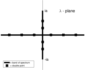
Figure 1: The Floquet spectrum of the Stokes wave with $\displaystyle\lfloor{aL}/{\pi}\rfloor=2.$

As the NLS spectrum is symmetric under complex conjugation, we subsequently only display the spectrum in the upper half $\lambda$-plane.

Novel instabilities of noneven solutions: Earlier work on perturbations of the NLS equation dealt primarily with solutions with even symmetry whose instabilities were identified solely via complex double points. In general, imposing symmetry on a solution restricts it’s dynamical behavior and may suppress instabilities. In the current damped HONLS experiments we find instabilities arise due to the asymmetry of the system that are not captured by complex double points. Although complex double points, if present in the damped HONLS flow, still identify instabilities, we need to develop a broader Floquet spectral characterization of instabilities to capture all the instabilities of noneven solutions.

A clue as to which new spectral elements are associated with instabilities in the full solution space of the NLS equation is provided by considering the following even 3-phase solution of the NLS [3],

$$u_{0}(x,t)=a\mathrm{e}^{2\mathrm{i}a^{2}t}\frac{\sqrt{\frac{\kappa}{1+\kappa}}\,\mbox{cn}\left(\frac{ax}{\sqrt{\kappa}},\sqrt{\frac{1-\kappa}{2}}\right)\,\mbox{dn}\left(\frac{a^{2}t}{\kappa},\kappa\right)+i\kappa\,\mbox{sn}\left(\frac{a^{2}t}{\kappa},\kappa\right)}{\sqrt{2}\kappa\left[1-\sqrt{\frac{\kappa}{1+\kappa}}\,\mbox{cn}\left(\frac{ax}{\sqrt{\kappa}},\sqrt{\frac{1-\kappa}{2}}\right)\mbox{cn}\left(\frac{a^{2}t}{\kappa},\kappa\right)\right]}.$$ (8)

With respect to $t$ the solution has a double frequency; a frequency determined by the exponential function and a modulation frequency determined by the elliptic functions. Formula (8) describes an even standing wave, periodic in space and time, arising as the degeneration of a 3-phase solution due to symmetry in it’s spectrum. The spatial period $L$ and temporal period $T$ are functions of $\mathcal{K}_{x}(\sqrt{\frac{1-\kappa}{2}})$ and $\mathcal{K}_{t}(\kappa)$, respectively, where $\mathcal{K}$ is the complete elliptic integral of the first kind. As $\kappa\rightarrow 1$ in (8), $T\rightarrow\infty$ and $u_{0}(x,t)\rightarrow U^{(1)}(x,t)$, the SPB given in Equation (10) associated with one complex double point.

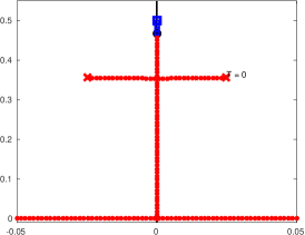
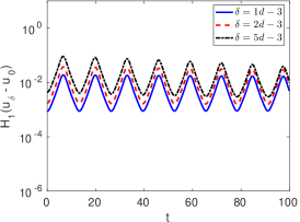
Figure 2: NLS cross state a) $|u_{0}(x,t)|$ for $0\leq t\leq 100$, b) it’s spectrum at $t=0$, c) $\eta(t)$ for $u_{\delta}(x,0)=u_{0}(x,0)+\delta g_{1}(x)$.

The surface and Floquet spectrum for $u_{0}(x,t)$ are shown in Figures 2A-B. The spectrum forms an even “cross” state with two bands of spectrum in the upper half plane with endpoints given by the simple periodic spectrum $\lambda_{0}=.5i$ and $\lambda_{1}^{\pm}=.35i\pm\alpha$. These two bands intersect transversally at $\lambda^{c}$ on the imaginary axis. Since $\partial\Delta/\partial\lambda=0$ at transverse intersections of bands of continuous spectrum, $\lambda^{c}$ is a critical point. There are no complex double points in $\sigma(u_{0}(x,t))$.

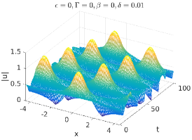
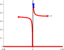
Figure 3: NLS noneven 3-phase solution a) $|u_{\delta}(x,t)|$ for $0\leq t\leq 100$, b) it’s spectrum at $t=0$, c) $\eta(t)$ for $u_{\delta}(x,0)=u_{0}(x,0)+\delta g_{2}(x)$.

To numerically address the stability of the cross state (8) with respect to initial data we consider small perturbations (both symmetric and asymmetric) of the following form:

$$u_{\delta}(x,0)=u_{0}(x,0)+\delta g_{k}(x),\quad k=1,2$$

where $g_{1}(x)=e^{i\phi}\cos\mu x$, $g_{2}(x)=e^{i\phi_{1}}\cos\mu x+re^{i\phi_{2}}\sin\mu x$, and $\delta=10^{-3},\dots,5\times 10^{-3}$. We examine i) the Floquet spectrum of $u_{\delta}(x,t)$ as compared with $u_{0}(x,t)$ and ii) the growth of the perturbations as $\delta$ is varied. We consider a solution $u(x,t)$ of the NLS equation to be stable if for every $\epsilon>0$ there exists a $\delta>0$ such that if $||u_{\delta}(x,0)-u(x,0)||_{H^{1}}<\delta$, then $||u_{\delta}(x,t)-u(x,t)||_{H^{1}}<\epsilon$, for all $t$. Therefore, to determine whether $u$ and $u_{\delta}$ stay close as time evolves, we monitor the evolution of the difference

$$\mathcal{\eta}(t)=||u_{\delta}(x,t)-u(x,t)||_{H^{1}}$$ (9)

where $||f||^{2}_{H^{1}}=\int_{-L/2}^{L/2}\left(|f_{x}|^{2}+|f|^{2}\right)\,dx.$

i) Symmetric perturbations of initial data: As $\phi$ and $\delta$ are varied, the surface and spectrum for $u_{\delta}(x,t)$ for perturbation $g_{1}(x)$ is qualitatively the same as in Figures 2A-B. The endpoints of the band of spectrum, $\sigma^{s}(u_{\delta})$, are slightly shifted maintaining even symmetry. Due to analyticity of $\Delta$, $\lambda^{c}$ does not split under even perturbations and the spectrum is not topologically different. Figure 2C shows the evolution of $\eta(t)$ for even perturbations $u_{\delta}(x,0)=u_{0}(x,0)+\delta g_{1}(x)$. The small osciallations in $\eta(t)$, typical in Hamiltonian systems, do not grow. The Floquet spectrum and the evolution of $\eta(t)$ show that when restricted to the subspace of even solutions, $u_{0}(x,t)$ is stable.

ii) Asymmetric perturbations of initial data: The surface and spectrum of $u_{\delta}(x,t)$ for $u_{\delta}(x,0)=u_{0}(x,0)+0.05\sin\mu x$ are shown in Figures 3A-B. A topologically different spectral configuration is obtained and the waveform is a modulated right traveling wave. The critical point $\lambda^{c}$ has split into $\lambda_{\pm}^{c}$ and the two disjoint bands of spectrum form a “right” state: the upper band with endpoints $\lambda_{0}^{s}$ and $\lambda_{1,\delta}^{+}$ in the right quadrant and the lower band with endpoint $\lambda_{1,\delta}^{-}$ extending to the real axis in the left quadrant. On the other hand, if e.g. $u_{\delta}(x,0)=u_{0}(x,0)+0.05(\cos\mu x+e^{i\pi/3}\sin\mu x)$, the waveform is a modulated left traveling wave. In this case the orientation of the bands of spectrum is reversed, forming a “left” state with the upper band in the left quadrant and the lower band in the right quadrant. As the parameters in $g_{2}(x)$ are varied these are the two possible noneven spectral configurations for $u_{\delta}(x,t)$. The perturbation analysis in Section 4 is related and shows noneven perturbations of the SPB split complex double points into left and right sates.

Figure 3C shows $\eta(t)$ grows to $\mathcal{O}(1)$ for asymmetric perturbations $u_{\delta}(x,0)=u_{0}(x,0)+\delta g_{2}(x)$. Clearly $u_{\delta}(x,t)$ does not remain close to $u_{0}(x,t)$ for these perturbations. We associate the transverse complex critical points with instabilities arising from symmetry breaking which are not excited when evenness is imposed. The exact nature of the instability associated with complex critical points is under investigation. The current damped HONLS experiments in Section 3 corroborate the significance of transverse critical points $\lambda^{c}$ in identifying instabilities in the unrestricted solution space.

2.2 Spatially periodic breather solutions of the NLS equation

The heteroclinic orbits of a spatially periodic unstable NLS potential $u(x,t)$ with complex double points, $\lambda^{d}_{j}$, in its Floquet spectrum can be derived using the Bäcklund-gauge transformation (BT) for the NLS equation [25]. Given a Stokes wave $u_{a}(t)$ with $N$ complex double points, a single BT of $u_{a}(t)$ at $\lambda^{d}_{j}$ yields the one mode SPB, $U^{(j)}(x,t)$, associated with the $j$-th UM, $1\leq j\leq N$. Introducing $\mu_{j}=2\pi j/L$, $\sigma_{j}=-2\mathrm{i}\mu_{j}\lambda_{j}$, $\cos p_{j}=\mu_{j}/2a$, and $\tau_{j}=(\rho-\sigma_{j}t)$ one obtains [3, 21]:

$$U^{(j)}(x,t)=a\mathrm{e}^{2\mathrm{i}a^{2}t}\left(\frac{\mathrm{i}\sin 2p_{j}\tanh\,\tau_{j}+\cos 2p_{j}-\sin p_{j}\cos\left(\mu_{j}x+\beta\right)\mbox{sech}\tau_{j}}{1+\sin p_{j}\cos\left(\mu_{j}x+\beta\right)\mbox{ sech }\tau_{j}}\right).$$ (10)

$U^{(j)}(x,t)$ exponentially approaches a phase shift of the Stokes wave, $\displaystyle\lim_{t\rightarrow\pm\infty}U^{(j)}(x,t)=ae^{2\mathrm{i}a^{2}t+\alpha_{\pm}}$, at a rate depending on $\lambda^{d}_{j}$. Figures 4A-B show the amplitudes of two distinct single mode SPBs, $U^{(1)}(x,t)$ and $U^{(2)}(x,t)$ over a Stokes waves with $N=2$ UMs. $U^{(1)}(x,t)$ and $U^{(2)}(x,t)$ are both unstable as the BT based at $\lambda_{j}$ saturates the instability of the $j$-th UM while the other instabilities of the background persist.

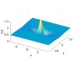
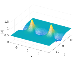
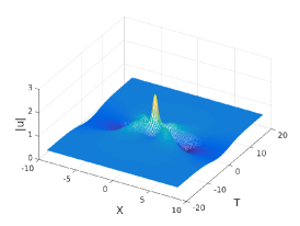
Figure 4: SPBs over a Stokes wave with $N=2$ UMs, $a=.5$, $L=4\sqrt{2}\pi$: Amplitudes of (a-b) single mode SPBs $|U^{(1)}(x,t,\rho)|$ and $|U^{(2)}(x,t,\rho)|$ ($\rho=\beta=0$) and (c) 2-mode SPB $|U^{(1,2)}(\rho,\tau)|$.

When the Stokes wave posesses two or more UMs, the BT can be iterated to obtain multi mode SPBs. For example, the two-mode SPB with wavenumbers $\mu_{i}$ and $\mu_{j}$, obtained by applying the BT successively at complex $\lambda_{i}^{d}$ and $\lambda_{j}^{d}$, is of the following form:

$$U^{(i,j)}(x,t;\rho,\tau)=a\mathrm{e}^{2\mathrm{i}a^{2}t}\frac{N(x,t;\rho,\tau)}{D(x,t;\rho,\tau)}.$$ (11)

The exact formula is provided in [6]. The parameters $\rho$ and $\tau$ determine the time at which the first and second modes become excited, respectively. Figure 4C shows the amplitude of the “coalesced” two mode SPB $U^{(1,2)}(x,t;\rho,\tau)$ ($\rho=-2$, $\tau=-3$) over a Stokes waves with $N=2$ UMs where the two modes are excited simultaneously.

An important property of the Bäcklund transformation: The BT is isospectral, i.e. $\sigma(u_{a}(t))=\sigma(U^{(j)}(x,t))=\sigma(U^{(i,j)}(x,t))$. For example, the Stokes wave with $N=2$ UMs (given in Figure 1) and each of the SPBs shown in Figures 4A-B-C share the same Floquet spectrum.

3 Numerical investigation of routes to stability of SPBs in the damped higher order NLS equation

In our examination of the even 3-phase solution in Section 2 we find that when evenness is relaxed novel instabilities arise which are associated with complex critical points. Armed with this result, in this section we return to the questions posed at the outset of our study: i) Which integrable instabilities are excited by the damped HONLS flow and what is the Floquet criteria for their saturation? ii) What remnants of integrable NLS structures are detected in the damped HONLS evolution?

The notation used in this section is as follows: i) The “$N$ UM regime” refers to the range of parameters $a$ and $L$ for which the underlying Stokes wave initially has $N$ unstable modes. ii) The initial data used in the numerical experiments is generated using exact SPB solutions of the integrable NLS equation. The perturbed SPBs are indicated with subscripts: $U^{(j)}_{\epsilon,\gamma}(x,t)$ refers to the solution of the damped HONLS Equation (1) for one-mode SPB initial data $U^{(j)}(x,0)$. Likewise $U^{(i,j)}_{\epsilon,\gamma}(x,t)$ is the solution to (1) for iterated SPB initial data.

The damped HONLS equation is solved numerically using a high-order spectral method due to Trefethen [19]. The integrator uses a Fourier-mode decomposition in space with a fourth-order Runge-Kutta discretization in time. The number of Fourier modes and the time step used depends on the complexity of the solution. For example, for initial data in the three UM regime, $N=1024$ Fourier modes are used with time step $\Delta t=7.5\times 10^{-5}$. As a benchmark the first three global invariants of the HONLS equation, the energy $E=\int_{0}^{L}|u|^{2}\,dx$, momentum $P=i\int_{0}^{L}\left(u^{*}u_{x}-uu_{x}^{*}\right)dx$, and Hamiltonian

$$H=\int_{0}^{L}\left\{-i|u_{x}|^{2}+i|u|^{4}-\frac{\epsilon}{4}\left(u_{x}u_{xx}^{*}-u_{x}^{*}u_{xx}\right)+2\epsilon|u|^{2}\left(u^{*}u_{x}-uu_{x}^{*}\right)+i\epsilon|u|^{2}\left[\mathcal{H}\left(|u|^{2}\right)\right]_{x}\right\}\,dx$$

are preserved with an accuracy of $\mathcal{O}(10^{-12})$ for $0\leq t\leq 100$. The invariant for the damped HONLS system, the spectral center $k_{m}=-P/2E$, is preserved with an accuracy of at least $\mathcal{O}(10^{-12})$ in the experiments.

Nonlinear mode decomposition of the damped HONLS flow: At each time $t$ we compute the spectral decomposition of the damped HONLS data using the numerical procedure developed by Overman et. al. [23]. After solving system (2), the discriminant $\Delta$ is constructed. The zeros of $\Delta\pm 2$ are determined using a root solver based on Müller’s method and then the curves of spectrum filled in. The spectrum is calculated with an accuracy of ${\mathcal{O}}(10^{-6})$ which is sufficient given the perturbation parameters $\epsilon$ and $\gamma$ used in the numerical experiments are ${\mathcal{O}}(10^{-2})$.

Notation used in the spectral plots: The periodic spectrum is indicated with a large $\times$ when $\Delta=-2$ and a large box when $\Delta=2$. The continuous spectrum is indicated with small $\times$ when the $\Delta$ is negative and a small box when $\Delta$ is positive.

Interpreting the damped HONLS flow via the NLS spectral theory: A tractable example which illustrates the use of the Floquet spectrum to interpret near integrable dynamics is the spatially uniform solution (there is no depenence on $\epsilon$) of the damped HONLS Equation (1),

$$u_{a,\gamma}(t)=a\mathrm{e}^{-\gamma t}\mathrm{e}^{\mathrm{i}(|a|^{2}\frac{(1-\mathrm{e}^{-2\gamma t})}{\gamma})}.$$ (12)

At a given time $t=t_{*}$ the nonlinear spectral decomposition of (12) can be explicitly determined by substituting $u_{a,\gamma}(t_{*})$ into $\mathcal{L}(u)\phi=\lambda\phi$. We find the periodic Floquet spectrum consists of $\lambda_{0}^{s}=\pm\mathrm{i}a\mathrm{e}^{-\gamma t_{*}}$ and infinitely many double points

$$(\lambda_{j}^{d})^{2}=\left(\frac{j\pi}{L}\right)^{2}-\mathrm{e}^{-2\gamma t_{*}}a^{2},\quad j\in\mathbb{Z},\quad j\neq 0,$$ (13)

where $\lambda_{j}^{d}$ is complex if $\left(\frac{j\pi}{L}\right)^{2}<\mathrm{e}^{-2\gamma t_{*}}a^{2}$. Under the damped HONLS evolution the endpoint of the band of spectrum $\lambda^{s}_{0}$ and the complex double points $\lambda^{d}_{j}$ move down the imaginary axis and then onto the real axis. Similarly, at $t=t_{*}$, a linearized stability analysis about $u_{a,\gamma}(t_{*})$ shows the growth rate of the $j$-th mode $\sigma_{j}^{2}=\mu_{j}^{2}\left(4\mathrm{e}^{-2\gamma t_{*}}a^{2}-\mu_{j}^{2}\right)$. Thus the number of complex double points and the number of unstable modes diminishes in time due to damping. As a result, $u_{a,\gamma}(t)$ stabilizes when the growth rate $\sigma_{1}=0$, i.e. when $\lambda_{1}^{d}=0$, giving $t_{*}=\frac{\ln(aL/\pi)}{\gamma}$.

Saturation time of the instabilities: Since the association of complex critical points with instabilities is a new result, we supplement the spectral analysis with an examination of the saturation time of the instabilities for the damped SPBs $U^{(j)}_{\epsilon,\gamma}(x,t)$ and $U^{(j,k)}_{\epsilon,\gamma}(x,t)$ as follows: we examine the growth of small asymmetric perturbations in the initial data of the following form,

$$U^{(j)}_{\epsilon,\gamma,\delta}(x,0)=U^{(j)}(x,0)+\delta f_{k}(x)$$

and

$$U^{(i,j)}_{\epsilon,\gamma,\delta}(x,0)=U^{(i,j)}(x,0)+\delta f_{k}(x)$$

where

i. $f_{k}(x)=\cos\mu_{k}x+r_{k}e^{i\phi_{k}}\sin\mu_{k}x$, $\mu_{k}=2\pi k/L$, $1\leq k\leq 3$,

ii. $f_{4}(x)=r(x)$, $r(x)\in[0,1]$ is random noise.

To determine the closeness of $U^{(j)}_{\epsilon,\gamma}(x,t)$ and $U^{(j)}_{\epsilon,\gamma,\delta}(x,t)$ as time evolves we monitor the evolution of $\eta(t)$, as given by Equation (9). We consider the solution to have stabilized under the damped HONLS flow once $\eta(t)$ saturates.

In the damped HONLS numerical experiments we obtain a new criteria for the saturation of instabilities: $\eta(t)$ saturates and the SPB stabilizes once damping eliminates all complex double points and complex critical points in the spectrum.

3.1 Damped HONLS SPB in the one unstable mode regime

1. $\bf U_{\epsilon,\gamma}^{(1)}(x,t)$ in the one UM regime: We begin by considering $U_{\epsilon,\gamma}^{(1)}(x,t)$ for $\epsilon=0.05$ and $\gamma=0.01$ in the one UM regime with initial data generated using Equation (10) with $j=1$, $a=0.5$ and $L=2\sqrt{2}\pi$. Figure 5A shows the surface $|U_{\epsilon,\gamma}^{(1)}(x,t)|$ for $0<t<100$.

    

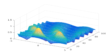
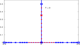
    A                                                        B

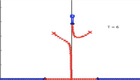
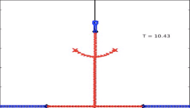
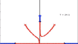
    C                                                        D                                                        E

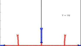
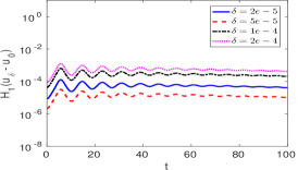
    F                                                        G

Figure 5: One UM regime: A) $|U_{\epsilon,\gamma}^{(1)}(x,t)|$ for $0\leq t\leq 100$ and the spectrum at B) $t=0$, C) $t=6$, D) $t=10.43$, E) $t=24.1$, F) $t=70$ and G) $\eta(t)$ for $f_{4}(x,t)$, $\delta=10^{-5},\dots,10^{-4}$ and $\epsilon=.05$, $\gamma=0.01$.

The evolution of the Floquet spectrum for $U_{\epsilon,\gamma}^{(1)}(x,t)$ is as follows: At $t=0$, the spectrum in the upper half plane consists of a single band of spectrum with end point at $\lambda_{0}^{s}=0.5\mathrm{i}$, indicated by a large “box”, and one imaginary double point at $\lambda_{1}^{d}=0.3535\mathrm{i}$, indicated by a large “$\times$” (Figure 5B). Under the damped HONLS $\lambda_{1}^{d}$ splits asymmetrically forming a right state, with the upper band of spectrum in the right quadrant and the lower band in the left quadrant, consistent with the short time perturbation analysis in Section 4. The right state is clearly visible at $t=6$ in Figure 5C with the waveform characterized by a single damped modulated mode traveling to the right. The spectrum persists in a right state with the separation distance between the two bands varying until $t=10.43$ when a cross state forms with an embedded critical point, Figure 5D, indicating an instability. Subsequently the critical point splits into a right state. As damping continues the band in the right quadrant widens, Figure 5E, and the vertex of the loop eventually touches the origin at $t\approx 27.5.$ The spectrum then has three bands emanating off the real axis, with endpoints $\lambda_{1}^{-},\lambda_{0}^{s},\lambda_{1}^{+}$ which, as damping continues, diminish in amplitude and move away from the imaginary axis, Figure 5F.

Figure 5G shows the evolution of $\eta(t)$ for $U_{\epsilon,\gamma}^{(1)}(x,t)$ using $f_{4}$ and $\delta=10^{-5},\dots,10^{-4}.$ The saturation of $\eta(t)$ at $t\approx 16$ is consistent with the Floquet criteria that the solution stabilizes after complex double points and complex critical points are eliminated in the damped HONLS flow.

From the spectral analysis of $U_{\epsilon,\gamma}^{(1)}(x,t)$ in the one UM regime, we find it may be characterized as a continuous deformation of a noneven generalization of the 3-phase solution, i.e. the right state (8). The amplitude of the oscillations of $U_{\epsilon,\gamma}^{(1)}(x,t)$ decreases and the frequency increases until small fast oscillations about the damped Stokes wave, visible in Figure 5A, are obtained.

3.2 Damped HONLS SPBs in the two unstable mode regime

For the two UM regime we let $a=0.5$, $L=4\sqrt{2}\pi$ ($N=\displaystyle\lfloor{aL}/{\pi}\rfloor=2$) and consider the two distinct perturbed single mode SPBs $U_{\epsilon,\gamma}^{(1)}(x,t)$ and $U_{\epsilon,\gamma}^{(2)}(x,t)$ and the perturbed iterated SPB $U_{\epsilon,\gamma}^{1,2}(x,t)$. The damped HONLS perturbation parameters are $\epsilon=0.05$ and $\gamma=0.01$.

1. $\bf U_{\epsilon,\gamma}^{(1)}(x,t)$ in the two UM regime: Figure 6A shows the surface $|U_{\epsilon,\gamma}^{(1)}(x,t)|$ for $0<t<100$ for initial data given by Equation (10) with $j=1$. The Floquet spectrum at $t=0$ is given in Figure 6B. The end point of the band of spectrum at $\lambda_{0}^{s}=0.5\mathrm{i}$ is indicated by a “box”. There are two complex double points at $\lambda_{1}^{d}=0.4677\mathrm{i}$ and $\lambda_{2}^{d}=0.3535\mathrm{i}$, indicated by a “$\times$” and “box”, respectively. For $t>0$ both double points split asymmetrically: $\lambda_{1}^{d}$, the complex double point at which $U^{(1)}(x,t)$ is constructed, splits at leading order into $\lambda_{1}^{\pm}$ such that a right state forms with the first mode traveling to the right. The second double point $\lambda_{2}^{d}$ splits at higher order into $\lambda_{2}^{\pm}$ such that a left state forms with the second mode traveling to the left. These disjoint asymmetric bands of spectrum are consistent with the short time perturbation analysis in Section 4 for damped HONLS data of the form (18).

    

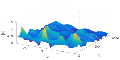
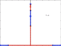
A                                                                             B

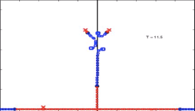
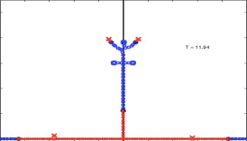
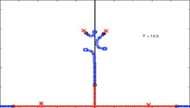
C                                                        D                                                        E

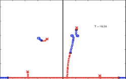
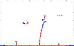
F                                                        G                                                        H

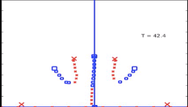
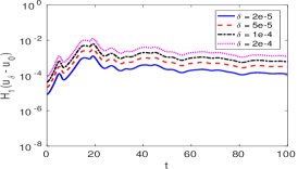
I                                                        J

Figure 6: Two UM regime: A) $|U_{\epsilon,\gamma}^{(1)}(x,t)|$ for $0\leq t\leq 100$, and spectrum at B) $t=0$, C) $t=11.5$, D) $t=11.94$, E) $t=12.5$, F) $t=19.26$, G) $t=19.32$, and H) $t=19.37$, I) $t=42.4$, and J) $\eta(t)$ for $f_{1}(x,t)$, $\delta=10^{-5},\dots,10^{-4}$.

This spectral configuration is representative of the spectrum during the initial stage of it’s evolution and is still observable in Figure 6C at $t=11.5$. A bifurcation occurs at $t=11.94$, Figure 6D, when a double cross state forms and two complex critical points emerge in the spectrum, indicating instabilities associated with both nonlinear modes. Subsequently both complex critical points split, Figure 6E, with the upper band in the left quadrant and the second band in the right quadrant corresponding to a damped waveform with the first mode traveling to the left and the second mode traveling to the right.

The bifurcation at $t=11.94$ corresponds to transitioning through the remnant of an unstable 5-phase solution (with two instabilities) of the NLS equation. The bands eventually become completely detached from the imaginary axis and a second complex critical point forms at $t=19.32$. The bifurcation sequence is shown in Figures 6F-G-H. The main band emanating from the real axis then reestablishes itself close to the imaginary axis, Figure 6I, and the spectrum settles into a configuration corresponding to a stable 5 phase solution. The bands move apart and downwards and hit the real axis with no further development of complex critical points. From the Floquet spectral perspective, once damping eliminates complex critical points in the spectrum at approximately $t\approx 20$, $U_{\epsilon,\gamma}^{(1)}(x,t)$ stabilizes.

Figure 6J shows the evolution of $\eta(t)$ for $U_{\epsilon,\gamma}^{(1)}(x,t)$ with $f_{2}$ for $\delta=10^{-5},\dots,10^{-4}.$ The perturbation $f_{2}$ is chosen in the direction of the unstable mode associated with $\lambda_{2}^{d}$. $\eta(t)$ stops growing by $t\approx 20$, confirming the instabilities associated with the complex critical ponts and time of stabilization obtained from the nonlinear spectral analysis.

For $U_{\epsilon,\gamma}^{(1)}(x,t)$ in the 2-UM regime, both $\lambda_{1}^{d}$ and $\lambda_{2}^{d}$ resonate with the perturbation. The route to stability is characterized by the appearance of the double cross state of the NLS and the proximity to this state is significant in organazing the damped HONLS dynamics. Once stabilized, $U_{\epsilon,\gamma}^{(1)}(x,t)$ may be characterized as a continuous deformation of a stable 5-phase solution.

2. $\bf U_{\epsilon,\gamma}^{(2)}(x,t)$ in the two UM regime: We now consider $U^{(2)}_{\epsilon,\gamma}(x,t)$ whose initial data is given by Equation (10) with $j=2$. Although $U^{(1)}(x,t)$ and $U^{(2)}(x,t)$ are both single mode SPBs over the same Stokes wave, their respective routes to stability under damping are quite different. Notice in Figure 7A the surface of $|U_{\epsilon,\gamma}^{(2)}(x,t)|$ for $0\leq t\leq 100$ is a damped modulated traveling state, exhibiting regular behavior, in contrast to the irregular behavior of $|U_{\epsilon,\gamma}^{(1)}(x,t)|$ in the two UM regime.

    

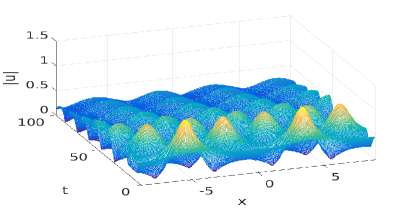
    A                                                        B

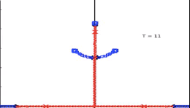
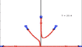
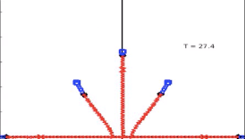
C                                                        D                                                        E

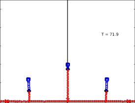
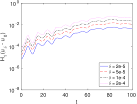
    F                                                        G

Figure 7: Two UM regime: A) $|U_{\epsilon,\gamma}^{(2)}(x,t)|$ for $0\leq t\leq 100$ and Spectrum at B) $t=6$. C) $t=11$, D) $t=23.4$, and E) $t=27.4$, F) $t=71.9$, and G) $\eta(t)$ for $f_{1}(x,t)$, $\delta=10^{-5},\dots,10^{-4}$ and $\gamma=0.01$.

The spectrum of $U_{\epsilon,\gamma}^{(2)}$ at $t=0$ is the same as in Figure 6B. Under perturbation $\lambda_{2}^{d}$ immediately splits asymmetrically into $\lambda^{\pm}_{2}$ with the upper band in the right quadrant and the lower band in the left quadrant, while the first double point $\lambda_{1}^{d}$ (indicated by the large “$\times$”) does not split. Figure 7B clearly shows that at $t=6$ damping has only split $\lambda_{2}^{d}$, i.e. the double point at which the SPB $U^{(2)}$ is constructed. In fact $\lambda_{1}^{d}$ does not split for the duration of the damped HONLS evolution, $0\leq t\leq 100$. In Figure 7C, by $t=11$, the two bands have aligned forming a cross state with a complex critical point at the transverse intersection of the bands while $\lambda_{1}^{d}$ is still intact and has simply translated down the imaginary axis.

The complex critical point subsequently splits with the upper band of spectrum again in the right quadrant, Figure 7D. Complex critical points do not reappear in the spectrum. At $t=27.4$ the vertex of the upper band of spectrum touches the real axis Figure 7E. As damping continues $\lambda_{1}^{d}$ moves down the imaginary axis and the two bands move away from the imaginary axis with diminishing amplitude. In Figure 7F the complex double point $\lambda_{1}^{d}$ has moved almost all the way down the imaginary axis. At $t\approx 76$, $\lambda_{1}^{d}=0$ and there are no complex double points in the subsequent spectral evolution.

We find $\eta(t)$ grows until $t=t_{s}\approx 80$, Figure 7G, consistent with the expectation that $U_{\epsilon,\gamma}^{(2)}$ will stabilize once all complex critical points and complex double points vanish in the spectrum. Until $\lambda^{d}_{1}$ moves onto the real axis, perturbations to the initial data $U_{\epsilon,\gamma,\delta}^{(2)}$ can excite the first mode associated with $\lambda^{d}_{1}$ causing $U_{\epsilon,\gamma}^{(2)}$ and $U_{\epsilon,\gamma,\delta}^{(2)}$ to grow apart.

Why doesn’t the HONLS perturbation split $\lambda_{1}^{d}$ when given $U^{(2)}(x,0)$ initial data? In Section 4, for short time, a suitable linearization of the damped HONLS SPB data is found to be given by Equation (19) for $j=1,2$, respectively where $\tilde{\epsilon}=\tilde{\epsilon}(\epsilon,\gamma)$. The perturbation analysis shows that at leading order damping only asymmetrically splits the double point $\lambda_{2}^{d}$ associated with $U^{(2)}(x,0)$. The endpoint of spectrum, $\lambda_{0}^{s}$, decreases in amplitude and the rest of the double points simply move along curves of continuous spectrum without splitting. The resonant modes which correspond to $\lambda_{2m}^{d}$ split asymmetrically at higher order $\mathcal{O}(\tilde{\epsilon}^{m})$. The splitting of $\lambda_{l}^{d}$, $l\neq 2m$, is beyond all orders in $\tilde{\epsilon}$ and is termed “closed”.

The spectral evolution for $U_{\epsilon,\gamma}^{(2)}(x,t)$ in the 2 UM regime is reminiscent of the spectral evolution of $U_{\epsilon,\gamma}^{(1)}(x,t)$ in the one UM regime. There is an important difference though: The nearby cross state that appears in the spectral decomposition of $U_{\epsilon,\gamma}^{(2)}(x,t)$ has two different types of instabilites: the instability associated with the complex critical point (potentially a phase instability) and the exponential instability associated with the (nonresonant) complex double point $\lambda_{1}^{d}$. The numerical results suggest that when nonresonant modes are present in the damped HONLS, their instabilities persist and organize the dynamics on a longer time scale. As $\lambda_{1}^{d}$ remains effectively closed for $t<t_{s}$, $U_{\epsilon,\gamma}^{(2)}(x,t)$ can be characterized as a continuous deformation of a noneven generalization of the degenerate 3 phase solution given by Equation (8) (the parameter values change due to doubling the period $L$; i,e. a $j-$th mode excitation with period L becomes a $2j-$th mode excitation with period 2$L$.)

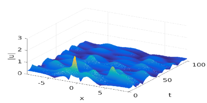
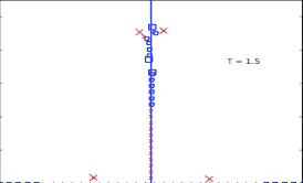
    A                                                        B

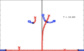
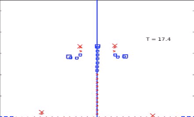
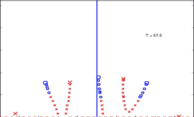
C                                                        D                                                        E

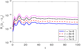
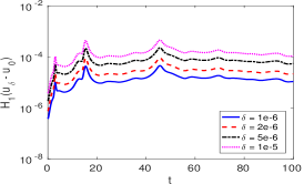
    F                                                        G

Figure 8: Two UM regime: A) $|U_{\epsilon,\gamma}^{(1,2)}(x,t)|$ for $0\leq t\leq 100$ and spectrum at B) $t=1.5$, C) $t=15.9$, D) $t=17.4$, E) $t=55$, and $\eta(t)$ for $U_{\epsilon,\gamma}^{(1,2)}(x,t)$ with $f_{1}(x,t)$ when F) $\rho=0,\tau=-2$ (the uncoalesced SPB), G) $\rho=0.665,\tau=1$ (the coalesced SPB).

3. $\bf U^{(1,2)}_{\epsilon,\gamma}(x,t)$ in the two UM regime: Figure 8A shows the surface $|U_{\epsilon,\gamma}^{(1,2)}(x,t)|$ for $0<t<100$ for initial data obtained from Equation (11) by setting $\rho=0$ and $\tau=-2$, $a=0.5$. The spectrum of $U_{\epsilon,\gamma}^{(1,2)}$ at $t=0$ is given by Figure 6B. As we’ve seen in the previous examples, once complex double points split they do not reform in the perturbed system; if they are present in the spectral decomposition of the damped HONLS, it is because the modes corresponding to $\lambda_{j}^{d}$ didn’t resonate under perturbation. Here both double points $\lambda^{d}_{1}$ and $\lambda^{d}_{2}$ split at leading order under the damped HONLS perturbation. Figure 8B shows for short time ($t=1.5$) the spectrum has a band gap structure indicating the first mode travels to the right and the second travels to the left. As time evolves the bands shift and align and Figure 8C shows at $t\approx 15.9$ two bands in the right quadrant intersect with an embedded complex critical point. The critical point splits with one band moving back towards the imaginary axis. There are now two bands detached from the primary band and moving downwards towards the real axis, Figures 8D-E. Complex critical points do not appear for $t>15.9$.

Figure 8F shows $\eta(t)$ for the example under consideration ($\rho=0,\tau=-2$) when $f_{1}(x,t)$,$\delta=10^{-5},\dots,10^{-4}$. We find $\eta(t)$ saturates at $t_{s}\approx 20$ indicating $U_{\epsilon,\gamma}^{(1,2)}$ has stabilized. For $t>t_{s}$ $U_{\epsilon,\gamma}^{(1,2)}$ is characterized as a continuous deformation of a stable NLS five-phase solution. The numerically observed initial splitting of complex double points $\lambda_{1}^{d}$ and $\lambda_{2}^{d}$ is consistent with the perturbation analysis of damped HONLS SPB data (19).

Among the two mode SPBs in the 2 UM regime, the one of highest amplitude due to coalescence of the modes appeared to be more robust [7]. An interesting observation is obtained if we examine the evolution of spectrum and of $\eta(t)$ using the initial data for the special coalesced two mode SPB, generated from Equation (11) by setting $\rho=0.665$, $\tau=1$, and $a=0.5$. For the coalesced case, complex critical points form 4 times for $0<t<45$ in the damped HONLS system. Figure 8G shows $\eta(t)$ saturates for $t\approx 50$. A comparison with the results of the non-coalesced two mode SPB given above indicate that remnants of the coalesced $U^{(1,2)}$ and it’s instabilities influence the damped HONLS dynamics over a longer time period, suggesting enhanced robustness with respect to perturbations of the NLS equation.

3.3 Damped SPBs in the three unstable mode regime

The parameters used for the three UM regime are $a=0.7$ and $L=4\sqrt{2}\pi$ ($N=\displaystyle\lfloor{aL}/{\pi}\rfloor=3$). The damped HONLS perturbation parameters are $\epsilon=0.05$ and $\gamma=0.01$. We present the results of two damped HONLS SPBs, $U_{\epsilon,\gamma}^{(2)}(x,t)$ and $U_{\epsilon,\gamma}^{2,3}(x,t)$, which exhibit an interesting or new feature. The evolutions of the other damped HONLS SPBs in the three UM regime in the three UM regime are discussed in relation to these cases.

    

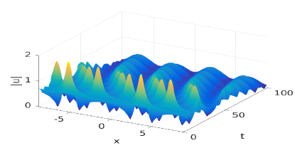
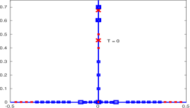
    A                                                        B

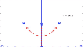
    C                                                        D

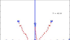
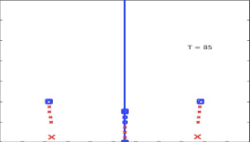
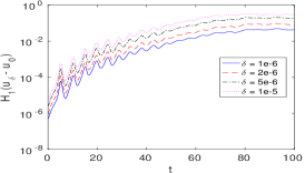
E                                                        F                                                        G

Figure 9: Three UM regime: A) $|U_{\epsilon,\gamma}^{(2)}(x,t)|$ for $0\leq t\leq 100$ and Spectrum at B) $t=0$, C) $t=4.7$, D) $t=36.6$, E) $t=42.8$, F) $t=85$ and G) $\eta(t)$ for $f_{1}(x,t)$, $\delta=10^{-6},\dots,10^{-5}$.

1. $\bf U_{\epsilon,\gamma}^{(2)}(x,t)$ in the three UM regime: The surface $|U_{\epsilon,\gamma}^{(2)}(x,t)|$ for initial data given by Equation (10) with $j=2$ is shown in Figure 9A for $0<t<100$. Notice in the 3 UM regime $U_{\epsilon,\gamma}^{(2)}(x,t)$ exhibits regular behavior and is a damped modulated right traveling wave as was $U_{\epsilon,\gamma}^{(2)}(x,t)$ in the 2 UM regime. The spectrum at $t=0$ is given in Figure 9B. The end point of the band of spectrum, $\lambda_{0}^{s}=0.7i$ is indicated by a “box”. There are three complex double points at $\lambda_{1}^{d}=0.677i$, $\lambda_{2}^{d}=0.604i$, and $\lambda_{3}^{d}=0.456i$ indicated by an “$\times$”, “box” and “$\times$”, respectively. Under the damped HONLS perturbation the complex double point at which $U_{\epsilon,\gamma}^{(2)}(x,t)$ is constructed, $\lambda_{2}^{d}$, splits into a right state as shown in Figure 9C. The complex double points $\lambda_{1}^{d}$ and $\lambda_{3}^{d}$ remain closed; $\lambda_{1}^{d}$ lies on the upper band in the right quadrant and $\lambda_{3}^{d}$ lies on the lower band. Transverse cross states with embedded complex critical points form frequently in the spectrum until $t\approx 68$, e.g. a cross state is shown at $t=36.6$ in Figure 9D. Figures 9E-F show the complex double points persist on the bands of spectrum until damping sufficiently diminishes the amplitude of the background and the complex double points reach the real axis at $t\approx 85$. In Figure 9G $\eta(t)$ saturates at $t=t_{s}\approx 90$. Due to the presence of the complex double points for $t<t_{s}$, $U_{\epsilon,\gamma}^{(2)}(x,t)$ can be viewed as a continuous deformation of an unstable 3 phase solution (with two instabilities). As discussed previously, the instabilities associated with the nonresonant modes persist longer than for the resonant modes.

In the 3 UM regime the behavior of the SPB $U_{\epsilon,\gamma}^{3}(x,t)$ is similar to $U_{\epsilon,\gamma}^{2}(x,t)$. In this case $\lambda_{3}^{d}$ initially splits asymmetrically into the right state (which we’ve now seen frequently in the initial damped HONLS system when only one mode is activated). The double points $\lambda_{1}^{d}$ and $\lambda_{2}^{d}$ do not split, they move along the band of spectrum created by $\lambda_{0}^{s}$ and $\lambda_{3}^{+}$. As a result $U_{\epsilon,\gamma}^{3}(x,t)$ stabilizes only when $\lambda_{1}^{d}$ and $\lambda_{2}^{d}$ become real, at $t\approx 140$. As in the previous cases, it is striking that the prediction from a short time perturbation analysis that certain double points remain closed, holds for the duration of the experiments (even while the solution evolves as a perturbed degenerate 3-phase state (with two instabilities). In contrast, for $U_{\epsilon,\gamma}^{1}(x,t)$ the higher order nonlinearities and damping excite all the modes. The solution is characterized by the formation of complex critical points and irregular behavior before stabilizing at $t\approx 40$.

2. $\bf U_{\epsilon,\gamma}^{(2,3)}(x,t)$ in the three UM regime: Figure 10A shows the surface $|U_{\epsilon,\gamma}^{(2,3)}(x,t)|$ for $0<t<100$ for initial data given by Equation (11) with $i,j=2,3$.

    

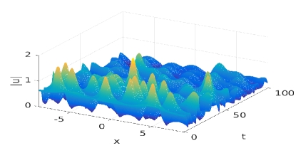
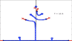
    A                                                        B

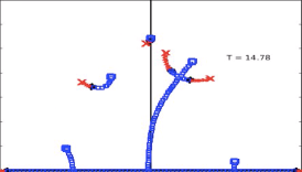
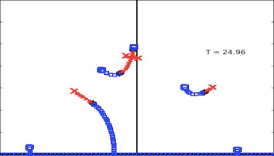
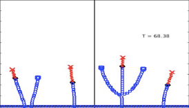
C                                                        D                                                        E

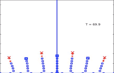
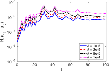
    F                                                        G

Figure 10: Three UM regime: A) $|U^{(2,3)}(x,t)|$ and Spectrum at B) $t=10.5$, C) $t=14.78$, D) $t=24.96$, E) $t=68.38$, F) $t=69.9$, and G) $\eta(t)$ for $f_{1}(x,t)$, $\delta=10^{-5},\dots,10^{-4}$ and $\gamma=0.01$.

The spectrum at $t=0$ is as in Figure 9B. The perturbation initially splits the double points $\lambda_{2}^{d}$ and $\lambda_{3}^{d}$ into $\lambda_{2}^{\pm}$ and $\lambda_{3}^{\pm}$ that correspond to a left and right modulated traveling modes, respectively. The new feature here is that the first complex double point, $\lambda_{1}^{d}$, splits at higher order into $\lambda_{1}^{\pm}$ (see the analysis in Section 4 showing that a multi-mode perturbation in a higher UM regime introduces new resonances not seen with single mode perturbations). The higher order splitting is visible in Figure 10B at $t=10.5$.

Complex double points are not observed in the spectral evolution for $t>0$.The formation of complex critical points in the spectrum occurs frequently as shown, for example, in Figure 10C and Figure 10D. Since the amplitude of the background state at $a=0.7$ is initially very close to the 4 UM regime, in this example we observe that nearby real double points are noticeably split by the perturbation. Figure 10E shows the spectrum at $t=68.4$ when the last complex critical point forms. This is reflected in Figure 10G which shows $\eta(t)$ saturates at $t_{s}\approx 68$. Each of the bursts of growth in $\eta(t)$ can be correlated with a complex critical point crossing. As time evolves disspiation diminshes the strength of the instability captured by the complex critical points or complex double points. $U_{\epsilon,\gamma}^{(2,3)}(x,t)$ exhibits quite rich and compex dynamics before damping saturates the instabilities and it’s behavior is not easy to characterize as when dealing with the perturbed SPBs in the $N=1,2$ UM regimes. For $t>t_{s}$ the evolution of $U_{\epsilon,\gamma}^{(2,3)}(x,t)$ may be characterized as a continuous deformation of a stable 7-phase solution (Figure 10F).

As a comparison, $U_{\epsilon,\gamma}^{(1,2)}(x,t)$ and $U_{\epsilon,\gamma}^{(1,3)}(x,t)$ exhibit shorter term irregular behavior with all the dominant modes excited and they stabilize at $t\approx 15,18$. respectively. $U_{\epsilon,\gamma}^{2,3}(x,t)$ was observed to take longer to stabilize due to the higher order splitting in $\lambda_{1}^{d}$.

The exact nature of the instability associated with complex critical points in under investigation. They may be weaker than the exponential instabilities associated with complex double points but the evolution of $U_{\epsilon,\gamma}^{(2,3)}(x,t)$ illustrates the their cumulative impact can be significant.

4 Perturbation Analysis

While examining the route to stability of the SPBs under the damped HONLS several novel results arose. One feature was that the instabilities of nonresonant modes persist longer than the instabilities of the resonant modes. We are interested in the fate of complex double points under noneven perturbations induced by HONLS as they characterize the SPB. Following the perturbation analysis in [1] used to determine the $\mathcal{O}(\epsilon)$ splitting of double points for single mode perturbations, we carry the analysis to higher order for noneven multi mode perturbations of the SPBs. We find i) additional modes resonate with the perturbation and ii) complex double points associated with nonresonant modes remain efffectively closed.

To obtain linearized initial conditions for the one and two mode SPBs we use the Hirota formulation of the SPBs [16]. For example for the one mode SPB one obtains,

$$u^{(j)}(x,t)=a\,e^{2\mathrm{i}a^{2}t}\,\frac{1+2\,\mathrm{e}^{2\mathrm{i}\theta_{j}+\Omega_{j}t+\gamma}\cos\mu_{j}x+A_{12}\,\mathrm{e}^{2(2\mathrm{i}\theta_{j}+\Omega_{j}t+\gamma)}}{1+2\,\mathrm{e}^{\Omega_{j}t+\gamma}\cos\mu_{j}x+A_{12}\,\mathrm{e}^{2(\Omega_{j}t+\gamma)}}$$ (14)

where $\mu_{j}=2\pi j/L$, $\Omega_{j}=\mu_{j}\sqrt{4a^{2}-\mu_{j}^{2}}$, $\sin\theta_{j}=\mu_{j}/2a$, $A_{12}=\sec^{2}\theta_{j}$, and $\gamma$ is an arbitrary phase.

The appropriate linearized initial conditions for the one and two mode SPBs, $u^{(i)}(x,0)$ and $u^{(i,j)}(x,0)$ respectively, are obtained by choosing $t$ and $\gamma$ such that $\tilde{\epsilon}_{s}=4\mathrm{i}\sin\theta_{s}\,\mathrm{e}^{\Omega_{s}t+\gamma}$, $s=i,j$, are small. After neglecting second-order terms we obtain:

$$u^{(j)}(x,0) = a\,\left(1+\tilde{\epsilon}_{j}\,\mathrm{e}^{\mathrm{i}\theta_{j}}\cos\mu_{j}x\right),$$ (15)

$$u^{(i,j)}(x,0) = a\,\left(1+\tilde{\epsilon}_{i}\,\mathrm{e}^{\mathrm{i}\theta_{i}}\cos\mu_{i}x+\tilde{\epsilon}_{j}\,\mathrm{e}^{\mathrm{i}\theta_{j}}\cos\mu_{j}x\right).$$ (16)

The damped HONLS yields the following noneven first order approximation for small time,

$$u^{(j)}(x,h) = a\left[1+\tilde{\epsilon}_{j}\left(\mathrm{e}^{\mathrm{i}\theta_{j}}\cos\mu_{j}x+r_{j}\,\mathrm{e}^{\mathrm{i}\phi_{j}}\sin\mu_{j}x\right)\right]$$ (17)

$$u^{(i,j)}(x,h) = a\left[1+\tilde{\epsilon}_{i}\,\left(\mathrm{e}^{\mathrm{i}\theta_{i}}\cos\mu_{i}x+r_{i}\,\mathrm{e}^{\mathrm{i}\phi_{i}}\sin\mu_{i}x\right)+\tilde{\epsilon}_{j}\,\left(\mathrm{e}^{\mathrm{i}\theta_{j}}\cos\mu_{j}x+r_{j}\mathrm{e}^{\mathrm{i}\phi_{j}}\sin\mu_{j}x\right)\right]$$ (18)

where $\theta_{s}\neq\phi_{s}$ and $a,\tilde{\epsilon}_{s},r_{s}$ are functions of $h$ and the damped HONLS parameters $\epsilon$ and $\gamma$, for $s=i,j$. For simplicity we set $\epsilon=\tilde{\epsilon}_{s}$ and suppress their explicit dependence on $\epsilon,\gamma$:

$$u=a+\epsilon\left[\mathrm{e}^{\mathrm{i}\theta_{i}}\cos\mu_{i}x+r_{i}\,\mathrm{e}^{\mathrm{i}\phi_{i}}\sin\mu_{i}x+Q\,\left(\mathrm{e}^{\mathrm{i}\theta_{j}}\cos\mu_{j}x+r_{j}\mathrm{e}^{\mathrm{i}\phi_{j}}\sin\mu_{j}x\right)\right]=a+\epsilon u^{(1)}$$ (19)

where $r_{s}\neq 0$ and $Q$ can be 0 or 1, depending on whether a one or two mode SPB is under consideration.

Since $\Delta(\lambda,u)$ and the eigenfunctions $v_{n}=\left[\begin{array}[]{l}v_{n1}\\ v_{n2}\end{array}\right]$ are analytic functions of their arguments, at the double points $\lambda_{n}$ we assume the following expansions:

$$v_{n} = v_{n}^{(0)}+\epsilon v_{n}^{(1)}+\epsilon^{2}v_{n}^{(2)}+\cdots$$ (20)

$$\lambda_{n} = \lambda_{n}^{(0)}+\epsilon\lambda_{n}^{(1)}+\epsilon^{2}\lambda_{n}^{(2)}+\cdots.$$ (21)

Substituting these expansions into Equation (29) we obtain the following:

$$\mathcal{O}(\epsilon^{0}):\quad\mathcal{L}v_{n}^{(0)} = 0$$ (22)

$$\mathcal{O}(\epsilon^{1}):\quad\mathcal{L}v_{n}^{(1)} = \left[\begin{array}[]{l}-\mathrm{i}\lambda_{n}^{(1)}v_{n1}^{(0)}+u^{(1)}v_{n2}^{(0)}\\ -\mathrm{i}\lambda_{n}^{(1)}v_{n2}^{(0)}+u^{(1)*}v_{n1}^{(0)}\end{array}\right]\equiv F$$ (25)

$$\mathcal{O}(\epsilon^{2}):\quad\mathcal{L}v_{n}^{(2)} = \left[\begin{array}[]{l}-\mathrm{i}\lambda_{n}^{(1)}v_{n1}^{(1)}-\mathrm{i}\lambda_{n}^{(2)}v_{n1}^{(0)}+u^{(1)}v_{n2}^{(1)}\\ -\mathrm{i}\lambda_{n}^{(1)}v_{n2}^{(1)}-\mathrm{i}\lambda_{n}^{(2)}v_{n2}^{(0)}+u^{(1)*}v_{n1}^{(1)}\end{array}\right]\equiv G.$$ (28)

where

$$\mathcal{L}=\left[\begin{array}[]{cc}\partial/\partial x+\mathrm{i}\lambda_{n}^{(0)}&-a\\ -a&-\partial/\partial x+\mathrm{i}\lambda_{n}^{(0)}\end{array}\right].$$ (29)

The leading order Equation (22) provides the spectrum for the Stokes wave. At the double points $\lambda_{n}^{(0)}$ the two dimensional eigenspace is spanned by the eigenfunctions

$$\phi_{n}^{\pm}=\mathrm{e}^{\pm\mathrm{i}k_{n}x}\left(\begin{array}[]{c}1\\ \frac{\mathrm{i}}{a}\left(\pm k_{n}+\lambda_{n}\right)\end{array}\right),$$ (30)

where $(\lambda_{n}^{(0)})^{2}=k_{n}^{2}-a^{2},k_{n}=n\pi/L$, and the general solution is given by

$$v_{n}^{(0)}=A^{+}\phi_{n}^{+}+A^{-}\phi_{n}^{-}$$ (31)

4.0.1 First order results

For periodic $v$, the solvability condition for the system $\mathcal{L}v=F=\left[\begin{array}[]{l}F_{1}\\ F_{2}\end{array}\right]$ is given by the orthogonality condition

$$\int_{0}^{L}\left(F_{1}w_{1}^{*}+F_{2}w_{2}^{*}\right)=0$$

for all $w$ in the nullspace of the Hermitian operator

$$\mathcal{L}^{H}=\left[\begin{array}[]{cc}-\partial/\partial x-\mathrm{i}\lambda_{n}^{*}&-a\\ -a&\partial/\partial x-\mathrm{i}\lambda_{n}^{*}\end{array}\right].$$ (32)

At the double points the nullspace of $\mathcal{L}^{H}$ is spanned by the eigenfunctions $\left(\begin{array}[]{l}\phi^{\pm}_{n2}\\ \phi^{\pm}_{n1}\end{array}\right)^{*}$ and the orthogonality condition becomes

$$\int_{0}^{L}\left(F_{1}\phi^{\pm}_{n2}+F_{2}\phi^{\pm}_{n1}\right)dx=0.$$ (33)

Applying this orthogonality condition to Equation (25) yields the system of equations

$$\left(\begin{array}[]{ll}T_{+}&T\\ T&T_{-}\end{array}\right)\left(\begin{array}[]{rr}A^{+}\\ A^{-}\end{array}\right)=0,$$ (34)

where

$$T = 2\lambda_{n}^{(0)}\lambda_{n}^{(1)}/a$$ (35)

$$T_{\pm} = -\mbox{$\frac{1}{2}$}\left\{\begin{array}[]{ll}\left(\frac{\pm k_{n}+\lambda_{n}}{a}\right)^{2}\left(\mathrm{e}^{\mathrm{i}\theta_{n}}\pm\mathrm{i}r_{n}\mathrm{e}^{\mathrm{i}\phi_{n}}\right)-\left(\mathrm{e}^{-\mathrm{i}\theta_{n}}\pm\mathrm{i}r_{n}\mathrm{e}^{-\mathrm{i}\phi_{n}}\right)&\quad n=i,j\\ 0&\quad n\neq i,j\end{array}\right..$$ (38)

Non trivial solutions $A^{\pm}$ are obtained only at the complex double points $\lambda_{n}$, $n=i,j$ at which the SPB was constructed providing the first order correction

$$\left(\lambda_{n}^{(1)}\right)^{2}=\left\{\begin{array}[]{ll}\frac{a^{2}}{4\lambda_{n}^{2}}\left[\sin(\omega_{n}+\theta_{n})\sin(\omega_{n}-\theta_{n})\right.&\\ \qquad+r_{n}^{2}\sin(\omega_{n}+\phi_{n})\sin(\omega_{n}-\phi_{n})&\quad n=i,j\\ \left.\qquad+\mathrm{i}r_{n}\sin(\phi_{n}-\theta_{n})\sin 2\omega_{n}\right]\\ 0&\quad n\neq i,j\end{array}\right.$$ (39)

where $\tan\omega_{n}=Im\left(\lambda_{n}^{(0)}\right)/k_{n}$ and $\theta_{s}\neq\phi_{s}\pm n\pi$ for $s=i,j$. As a result $\lambda_{n}^{(1,\pm)}=\pm r^{1/2}\mathrm{e}^{ip/2}$ where $0<p<2\pi$ and the double point splits asymmetrically in any direction. Examining $\Delta$ in a neighborhood of $u^{(0)}$ we find that when $u^{(1)}$ resonates with a particular mode, the band of continuous spectrum along the imaginary axis splits asymmetrically into two disjoint bands in the upper half plane. The other double points do not experience an $\mathcal{O}(\epsilon)$ correction.

The spectral configuration is determind by the location of $\lambda_{n}^{(\pm)}=\lambda^{(0)}+\epsilon\lambda^{(1,\pm)}$. $\lambda_{n}^{+}$ determines the speed and direction of the associated phase. For example, in the one complex double point regime there are only two spectral configurations associated with noneven perturbation: i) For $0<p<\pi$, Re $\lambda^{+}>0$ and the upper band of spctrum lies in the first quadrant. The wave form is characterized by a single modulated mode traveling to the right. ii) For $\pi<p<2\pi$, Re $\lambda^{+}<0$, the upper band of spectrum is in the second quadrant, and the wave form is characterized by a single modulated mode traveling to the left.

As seen in the numerical experiments, for noneven perturbations under the damped HONLS, the evolution of spectrum between two distinct configurations occurs when the continuous spectrum forms transverse bands with a complex ctitical point (not double point) and then splits.

4.0.2 Second order results

Determining the $\mathcal{O}(\epsilon^{2})$ corrections to the double points $\lambda_{n}$ for $n\neq i,j$, requires determining the eigenfunctions at $\mathcal{O}(\epsilon)$. When $\lambda_{n}^{(1)}=0$ the right hand side of Equation (25) simplifies to

$$\mathcal{L}v_{n}^{(1)}=\mathcal{F}=\left[\begin{array}[]{rr}0&u^{(1)}\\ u^{(1)*}&0\end{array}\right]v_{n}^{(0)}=\left[\begin{array}[]{r}u^{(1)}\left(A^{+}\phi_{n2}^{+}+A^{-}\phi_{n2}^{-}\right)\\ u^{(1)*}\left(A^{+}\phi_{n1}^{+}+A^{-}\phi_{n1}^{-}\right)\end{array}\right]$$

where $\phi_{n}^{\pm}$ is given by Equation (30). We assume $v_{n}^{(1)}=v_{n}^{(0)}+\sum_{n}^{(1)}$ where

$$\begin{array}[]{rcl}\sum_{n}^{(1)}&=&\mathbf{A}_{i}\mathrm{e}^{\mathrm{i}(k_{n}+\mu_{i})x}+\mathbf{B}_{i}\mathrm{e}^{\mathrm{i}(k_{n}+\mu_{i})x}+\mathbf{C}_{i}\mathrm{e}^{-\mathrm{i}(k_{n}-\mu_{i})x}+\mathbf{D}_{i}\mathrm{e}^{-\mathrm{i}(k_{n}+\mu_{i})x}\\ &&+\mathbf{A}_{j}\mathrm{e}^{\mathrm{i}(k_{n}+\mu_{j})x}+\mathbf{B}_{j}\mathrm{e}^{\mathrm{i}(k_{n}-\mu_{j})x}+\mathbf{C}_{j}\mathrm{e}^{-\mathrm{i}(k_{n}-\mu_{j})x}+\mathbf{D}_{j}\mathrm{e}^{-\mathrm{i}(k_{n}+\mu_{j})x}.\end{array}$$ (40)

Substituting $\sum_{n}^{(1)}$ into Equation (25) we find the coefficient vectors to be (with $n\neq s$, $s=i,j$)

$$\mathbf{A}_{s}=\frac{A^{+}/2}{\mu_{s}^{2}+2k_{n}\mu_{s}}\left[\begin{array}[]{c}\frac{1}{a}\left[(2(\cos\theta_{s}-\sin\phi_{s})a^{2}+\left(\mathrm{e}^{\mathrm{i}\theta_{s}}+i\mathrm{e}^{\mathrm{i}\phi_{s}}\right)\left(k_{n}+\lambda_{n}\right)\mu_{s}\right]\\ \mathrm{i}\left[2(\cos\theta_{s}-\sin\phi_{s})(k_{n}+\lambda_{n})+\left(\mathrm{e}^{\mathrm{i}\theta_{s}}-i\mathrm{e}^{\mathrm{i}\phi_{s}}\right)\mu_{s}\right]\end{array}\right]\\$$

$$\mathbf{B}_{s}=\frac{A^{+}/2}{\mu_{s}^{2}-2k_{n}\mu_{s}}\left[\begin{array}[]{c}\frac{1}{a}\left[(2(\cos\theta_{s}-\sin\phi_{s})a^{2}-\left(\mathrm{e}^{\mathrm{i}\theta_{s}}+i\mathrm{e}^{\mathrm{i}\phi_{s}}\right)\left(k_{n}+\lambda_{n}\right)\mu_{s}\right]\\ \mathrm{i}\left[2(\cos\theta_{s}-\sin\phi_{s})(k_{n}+\lambda_{n})-\left(\mathrm{e}^{\mathrm{i}\theta_{s}}-i\mathrm{e}^{\mathrm{i}\phi_{s}}\right)\mu_{s}\right]\end{array}\right]\\$$

$$\mathbf{C}_{s}=\frac{A^{-}/2}{\mu_{s}^{2}-2k_{n}\mu_{s}}\left[\begin{array}[]{c}\frac{1}{a}\left[(2(\cos\theta_{s}-\sin\phi_{s})a^{2}+\left(\mathrm{e}^{\mathrm{i}\theta_{s}}+i\mathrm{e}^{\mathrm{i}\phi_{s}}\right)\left(-k_{n}+\lambda_{n}\right)\mu_{s}\right]\\ \mathrm{i}\left[2(\cos\theta_{s}-\sin\phi_{s})(-k_{n}+\lambda_{n})+\left(\mathrm{e}^{\mathrm{i}\theta_{s}}-i\mathrm{e}^{\mathrm{i}\phi_{s}}\right)\mu_{s}\right]\end{array}\right]\\$$

$$\mathbf{D}_{s}=\frac{A^{-}/2}{\mu_{s}^{2}+2k_{n}\mu_{s}}\left[\begin{array}[]{c}\frac{1}{a}\left[(2(\cos\theta_{s}-\sin\phi_{s})a^{2}-\left(\mathrm{e}^{\mathrm{i}\theta_{s}}+i\mathrm{e}^{\mathrm{i}\phi_{s}}\right)\left(-k_{n}+\lambda_{n}\right)\mu_{s}\right]\\ \mathrm{i}\left[2(\cos\theta_{s}-\sin\phi_{s})(-k_{n}+\lambda_{n})-\left(\mathrm{e}^{\mathrm{i}\theta_{s}}-i\mathrm{e}^{\mathrm{i}\phi_{s}}\right)\mu_{s}\right]\end{array}\right]\\$$

With $v_{n}^{(1)}$ in hand, applying the orthogonality condition to Equation (28) yields the system

$$\left[\begin{array}[]{cc}\alpha_{n}^{+}&\lambda_{n}^{(2)}-\beta_{n}\\ \lambda_{n}^{(2)}-\beta_{n}&\alpha_{n}^{-}\end{array}\right]\left[\begin{array}[]{c}A^{+}\\ A^{-}\end{array}\right]=0$$ (41)

giving an $\mathcal{O}(\epsilon^{2})$ correction of the form

$$\left(\lambda_{n}^{(2)}-\beta_{n}\right)^{2}=\left\{\begin{array}[]{ll}\alpha_{n}^{+}\alpha_{n}^{-}&\quad n=2i,2j,i+j,j-i\\ &\\ 0&\quad\mbox{for all other cases}\end{array}\right.$$ (42)

Consequently only the double points $\lambda_{n}^{(0)}$ with $n=2i,2j,i+j$, or $j-i$ experience an $\mathcal{O}(\epsilon^{2})$ splitting. All other double points experience an $\mathcal{O}(\epsilon^{2})$ translation. This calculation can be carried to higher order $\mathcal{O}(\epsilon^{m})$. In the simpler case of a damped single mode SPB, $U_{\epsilon,\gamma}^{(j)}(x,t)$, only $\lambda_{n}^{(0)}$ corresponding to the resonant mode $n=mj$ will split at order $\mathcal{O}(\epsilon^{m})$ whereas the splitting is beyond all orders for $\lambda_{n}^{(0)}$, $n\neq mj$ [2].

For the two mode damped SPB $U_{\epsilon,\gamma}^{(2,3)}$ in the 3 UM regime we find $\lambda_{2}^{d}$ and $\lambda_{3}^{d}$ will split at $\mathcal{O}(\epsilon)$. The mode associated with $\lambda_{1}^{(0)}$ resonates also with $u^{(1)}$ at $\mathcal{O}(\epsilon^{2})$. All 3 complex double points split, in contrast with one mode $U_{\epsilon,\gamma}^{(2)}$ where $\lambda_{1}^{(0)}$ and $\lambda_{3}^{(0)}$ do not split.

5 Conclusions

In this paper we investigated the route to stability for single and multi-mode SPBs (which are even solutions of the NLS equation) in the framework of a damped HONLS equation using the Floquet spectral theory of the NLS equation. We found novel instabilities emerging in the symmetry broken solution space of the damped HONLS which are not captured by complex double points in the Floquet spectrum. To develop a broadened Floquet characterization of instabilities we examined the stability of an even 3-phase solution of the NLS equation with respect to noneven perturbations. We found the transverse complex critical point in its spectrum is associated with an instability arising from symmetry breaking which is not excited when evenness is imposed.

The association of instabilities due to symmetry breaking with complex critical points of the Floquet spectrum was corroborated by the numerical experiments. If one of the complex double points present at $t=0$ splits in the damped HONLS system, the subsequent spectral evolution involves repeated formation and splitting of complex critical points (not double points) which we correlated with the observed instabilities.

In the numerical study we presented experiments using fixed values of the perturbation parameters $\epsilon$ and $\gamma$. As these parameters are varied fewer or more critical points may form and the time the damped HONLS solution stabilizes may vary but the following interesting results are independent of their specific value: i) Instabilities due to symmetry breaking are associated with complex critical points. ii) Solutions stabilize once damping eliminates all the complex critical points and complex double points in the spectral deomposition of the damped HONLS data. iii) Only certain modes resonate with the damped HONLS perturbation. Resonant modes aid in stabilizing the solution. If nonresonant modes are present, their instabilities persist and appear to organize the dynamics on a longer timescale.

Each burst of growth in $\eta(t)$ can be correlated with the emergence of a complex critical point. The numerics suggest the instabilities associated with complex critical points may be weaker than those associated with complex double points. Even so the exact nature of the instability is warrants further investigation. As demonstrated by the evolution of $U_{\epsilon,\gamma}^{(2,3)}(x,t)$ their cumulative impact can be significant.

A perturbation analysis is presented to confirm the splitting of the initial complex double points observed in the numerical experiments. We find that certain complex double points present in the SPB initial data do not split under the damped HONLS flow. This short time analysis prediction holds for the duration of the experiments, even though the solution evolves as a damped multi-phase state.

Funding

This work was partially supported by Simons Foundation, Grant #527565

References

- [1] M. J. Ablowitz, B. M. Herbst, and C. M. Schober. Computational chaos in the nonlinear schrödinger equation without homoclinic crossings. Physica A, 228:212–235, 1996.
- [2] M. J. Ablowitz and C. M. Schober. Effective chaos in the nonlinear schrödinger equation. Contemporary Mathematics, 172:253, 1994.
- [3] N. N. Akhmediev, V. M. Eleonskii, and N. E. Kulagin. Exact first-order solutions of the nonlinear schrödinger equation. Theor. Math. Phys. (USSR), 72:809–818, 1987.
- [4] N. N. Akhmediev, J. M. Soto-Crespo, and A. Ankiewicz. Extreme waves that appear from nowhere: on the nature of rogue waves. Phys. Lett. A, 373:2137–2145, 2009.
- [5] T. B. Benjamin and J. E. Feir. The disintegration of wave trains in deep water. J. Fl. Mech., 27:417–430, 1967.
- [6] A. Calini and C. M. Schober. Homoclinic chaos increases the likelihood of rogue wave formation. Phys. Lett. A, 298:335–349, 2002.
- [7] A. Calini and C. M. Schober. Numerical investigation of stability of breather-type solutions of the nonlinear schrödinger equation. Nat. Haz. and Earth Sys. Sci., 14:1431–1440, 2014.
- [8] A. Calini and C. M. Schober. Characterizing jonswap rogue waves and their statistics via inverse spectral data. Wave Motion, 71:5–17, 2017.
- [9] A. Chabchoub, N. P. Hoffmann, and N. Akhmediev. Rogue wave observation in a water wave tank. Phys. Rev. Lett., 106:1–4, 2011.
- [10] Pelinovsky D Chen J. Rogue periodic waves of the focusing nonlinear schrödinger equation. Proc. Roy. Soc. A, 474, 2018.
- [11] Segal BL Deconinck B. The stability spectrum for elliptic solutions to the focusing nls equation. Physica D, 346:1–19, 2017.
- [12] Solli DR, Ropers C, Koonath P, and Jalali B. Optical rogue waves. Nature, 450, 2007.
- [13] K. B. Dysthe and K. Trulsen. Note on breather type solutions of the nls as models for freak-waves. Physica Scripta, T82:48–52, 1999.
- [14] N. Ercolani, M. G. Forest, and D. W. McLaughlin. Geometry of the modulational instability. iii. homoclinic orbits for the periodic sine-gordon equation. Physica D, 43:349–384, 1990.
- [15] G. Fotopoulos, D. J. Frantzeskakis, N. I. Karachalios, P. G. Kevrekidis, V. Koukouloyannis, and K. Vetas. Extreme wave events for a nonlinear schrödinger equation with linear damping and gaussian driving. arXiv: 1812.05439, 2019.
- [16] R. Hirota. Lecture Notes in Mathematics 515. Springer-Verlag, New York, 1976.
- [17] Slunyaev A Kharif C, Pelinovsky E. Rogue Waves in the Ocean. Springer-Verlag, Berlin Heidelberg, 2009.
- [18] B. Kibbler, J. Fatome, C. Finot, G. Millot, F. Dias, G. Genty, N. Akhmediev, and J. Dudley. The peregrine soliton in nonlinear fibre optics. Nature Physics, 6:790–795, 2010.
- [19] Trefethen LN. Spectral Methods. SIAM, Philadelphia, 2000.
- [20] Onorato M, Residori S, Bortolozzo U, Montina A, and Arecchi FT. Rogue waves and their generating mechanisms in different physical contexts. Physics Reports, 528:47–89, 2013.
- [21] D. W. McLaughlin and E. A. Overman. Whiskered tori for integrable pdes and chaotic behavior in near integrable pdes. Surv. Appl. Math., 1:83–203, 1995.
- [22] A. Osborne, M. Onorato, and M. Serio. The nonlinear dynamics of rogue waves and holes in deep-water gravity wave train. Phys. Lett. A, 275:386–393, 2000.
- [23] Bishop AR Overman II EA, McLaughlin DW. Coherence and chaos in the driven damped sine-gordon equation: measurement of the soliton spectrum. Physica D, 19:1–41, 1986.
- [24] D. Peregrine. Water waves, nonlinear schrödinger equations and their solutions. J. Austral. Math. Soc. Ser. B, 25:16–43, 1983.
- [25] D. H. Sattinger and V. D. Zurkowski. Gauge theory of bäcklund transformations. ii. Physica D, 26:225–250, 1987.
- [26] C. M. Schober and A. L. Islas. The routes to stability of spatially periodic solutions of the linearly damped nls equation. The European Physical Journal Plus, 135:1–20, 2020.
- [27] H. Segur, D. Henderson, J. Carter, J. Hammack, C. Li, D. Pheiff, and K. Socha. Stabilizing the benjamin-feir instability. J. Fluid Mech., 539:229–271, 2005.
- [28] G. G. Stokes. On the theory of oscillatory waves. Camb. Trans., 8:441–473, 1847.
- [29] V. E. Zakharov. Stability of periodic waves of finite amplitude on the surface of a deep fluid. J. Appl. Mech. and Tech. Phys., 9:190–194, 1968.
- [30] V. E. Zakharov and A. B. Shabat. Exact theory of two-dimensional self-focusing and onedimensional self-modulation of waves in nonlinear media. Soviet Phys. JETP, 34:62–69, 1972.
- [31] C. Zaug and J. D. Carter. Dissipative models of swell propagation across the pacific. arXiv: 2005.06635, 2020.