Message-Aware Graph Attention Networks for Large-Scale Multi-Robot Path Planning

Abstract

The domains of transport and logistics are increasingly relying on autonomous mobile robots for the handling and distribution of passengers or resources. At large system scales, finding decentralized path planning and coordination solutions is key to efficient system performance. Recently, Graph Neural Networks (GNNs) have become popular due to their ability to learn communication policies in decentralized multi-agent systems. Yet, vanilla GNNs rely on simplistic message aggregation mechanisms that prevent agents from prioritizing important information. To tackle this challenge, in this paper, we extend our previous work that utilizes GNNs in multi-agent path planning by incorporating a novel mechanism to allow for message-dependent attention. Our Message-Aware Graph Attention neTwork (MAGAT) is based on a key-query-like mechanism that determines the relative importance of features in the messages received from various neighboring robots. We show that MAGAT is able to achieve a performance close to that of a coupled centralized expert algorithm. Further, ablation studies and comparisons to several benchmark models show that our attention mechanism is very effective across different robot densities and performs stably in different constraints in communication bandwidth. Experiments demonstrate that our model is able to generalize well in previously unseen problem instances, and that it achieves a 47% improvement over the benchmark success rate, even in very large-scale instances that are $\times$100 larger than the training instances.

I Introduction

Remarkable progress has been achieved for Multi-Robot Path Planing [1, 2, 3, 4]—a problem that considers the generation of collision-free paths leading robots from their start positions to designated goal positions. In recent years, solutions to this problem have become increasingly important for item retrieval in warehouses [5] and mobility-on-demand services [6].

However, computing a solution that can balance between optimality and real-world efficiency remains a challenge. Current approaches can be mainly classified into centralized and decentralized. Centralized methods require central units to gather information from all robots and organize the optimal path for each of them, consuming large computational resources. As the system scales, decentralized approaches become increasingly popular, where each robot estimates or communicates others’ future trajectories via broadcasting or distance-based communication. Unfortunately, if the communication happens concurrently and equivalently among many neighboring robots, it is likely to cause redundant communication, burden the computational capacity and adversely affect overall team performance. Besides, robust and continuous communication cannot yet be guaranteed due to limited bandwidth, large data volumes, and interference from the surroundings. Additionally, under a fully decentralized framework without any priority of planning, it is very hard to ensure the convergence of the negotiation process [7]. These limitations ultimately affect the optimality of solutions found and the overall resilience of the team to disruptions. Hence, new trends of research focus on communication-aware path planning approaches by explicitly considering communication efficiency during path generation and path optimization [8], addressing to whom the information is communicated, and at what time [9].

Contributions. In this work, we propose to use a Message Aware Graph Attention neTwork (MAGAT) to extend our previous decentralized framework [4]. Our contributions are summarized as follows:

• We combine a Graph Neural Network (GNN) with a key-query-like attention mechanism to improve the effectiveness of inter-robot communication. We demonstrate the suitability of applying our model on dynamic communication graphs by proving its permutation equivariance and time invariance property.

• We investigate the impact of reduced communication bandwidth by reducing the size of the shared features, and then deploy a skip-connection to preserve self-information and maintain model performance.

• We demonstrate the generalizability of our model by training the model on small problem instances and testing it on increasing robot density, varying map size, and much larger problem instances (up to $\boldsymbol{\times 100}$ the number of robots). Our proposed model is shown to be more efficient in learning general knowledge of path planning as it achieves better generalization performance than the baseline systems under various scenarios.

II Related Work

Learning-based methods have been actively investigated in recent years, and have demonstrated their strengths in designing robot control policies for an increasing number of tasks [10]. These methods have shown their capabilities to offload the online computational burden into an offline learning procedure, which allows agents to act independently based on the learned knowledge, and thus to work in a decentralized manner [3, 11]. Sartoretti et al. [3] have proposed a hybrid learning-based method called PRIMAL for multi-agent path-finding that integrated imitation learning (via an expert algorithm) and multi-agent reinforcement learning. Their approaches did not consider inter-robot communication, and thus, did not exploit the full potentials of the decentralized system.

Communication between robots is essential, especially for decentralized approaches. Addressing the problems of what information should be sent to whom and when is crucial to solving the task effectively. Early works have explored discrete communication, through signal binarization [12] or variable-length coding scheme [13], and compositional language using abstract discrete symbols for categorical communication emissions in a grounded communication environment [14]. Our previous work [4] developed a decentralized framework for multi-agent coordination in partially observed environments based on Graph Neural Networks (GNNs) to achieve explicit inter-robot communication. However, we did not investigate whether it is actually beneficial to weigh features received from neighboring robots before making decisions.

Attention mechanisms. GNNs have attracted increasing attention in various fields, including the multi-robot domain (flocking and formation control [15], and multi-robot path planning [4]). However, how to effectively process large-scale graphs with noisy and redundant information is still under active investigation. A potential approach is to introduce attention mechanisms to actively measure the relative importance of node features. Hence, the network can be trained to focus on task-relevant parts of the graph [16]. Learning attention over static graphs has been proved to be efficient. Besides, Liu et al. [17] developed a learning-based communication model that constructed the communication group on a static graph to address what to transmit and which agent to communicate for collaborative perception. However, its permutation equivariance, time invariance and its practical effectiveness in dynamic multi-agent communication graphs have not yet been verified.

III Problem Formulation

Problem. We set up a 2D grid world $\mathcal{W}$, which contains a set of static obstacles $\mathcal{C}\subset\mathcal{W}$. Let ${\mathcal{V}}=\{v_{1},\ldots,v_{N}\}$ be the set of $N$ robots with independent pairs of the start and goal positions. We formulate the multi-agent path planning problem as a sequential decision-making problem, where, at every time instant $t$, each robot $i$ takes an action ${\tilde{\mathbf{u}}}_{t}^{i}$ towards its goal in a collision-free path, given the following assumptions.

Assumptions. 1) There is no global positioning of the robots. The map perceived by robot $i$ at time $t$ is denoted by ${\mathbf{M}}_{t}^{i}\in{\mathbb{R}}^{W_{\mathrm{FOV}}\times H_{\mathrm{FOV}}}$, where $W_{\mathrm{FOV}}$ and $H_{\mathrm{FOV}}$ are the width and height (in 2D plane) of the rectangular Field of View (FOV). 2) When the goal of the robot is outside the FOV, this information is clipped to the FOV boundary in a local reference frame (see Fig. 1), resulting in only the awareness of the direction of its goal. 3) Compared with the time for the robot’s movement, the communication between the neighboring robots happens instantly without delay, and is not blocked by any static obstacles $\mathcal{C}$. 4) We further limit the communication such that robots can only send out their features at a specific bandwidth, but cannot access the ownership of the feature received.

Communications. Each robot can communicate, or share information with only adjacent robots. We formalize this communication with a dynamic distance-based communication network. We can describe this network at time $t$ by means of a graph ${\mathcal{G}}_{t}=({\mathcal{V}},{\mathcal{E}}_{t},{\mathcal{W}}_{t})$ where ${\mathcal{V}}$ is the set of robots, ${\mathcal{E}}_{t}\subseteq{\mathcal{V}}\times{\mathcal{V}}$ is the set of edges and ${\mathcal{W}}_{t}:{\mathcal{E}}_{t}\to{\mathbb{R}}$ is a function that assigns weights to the edges. The graph is distance-based because robots $v_{i}$ and $v_{j}$ can communicate with each other at time $t$ if and only if $(v_{i},v_{j})\in{\mathcal{E}}_{t}$. For instance, two robots $v_{i}$ and $v_{j}$, with positions ${\mathbf{p}}_{i},{\mathbf{p}}_{j}\in{\mathbb{R}}^{2}$ respectively, can communicate with each other if $\|{\mathbf{p}}_{i}-{\mathbf{p}}_{j}\|\leq r_{\mathrm{COMM}}$ for a given fixed communication radius $r_{\mathrm{COMM}}>0$. This allows us to define an adjacency matrix ${\mathbf{S}}_{t}\in{\mathbb{R}}^{N\times N}$ representing the distance-based communication graph, where $[{\mathbf{S}}_{t}]_{ij}=s_{t}^{ij}=0$ if $(v_{i},v_{j})\notin{\mathcal{E}}_{t}$ and $1$ otherwise. The corresponding edge weight ${\mathcal{W}}_{t}(v_{i},v_{j})=w_{t}^{ij}=[{\mathbf{S}}_{t}]_{ij}[E]_{ij}\in[0,1]$, where $[{\mathbf{S}}_{t}]_{ij}$ represents the graph connectivity and $[E]_{ij}$ (will be introduced later in Eq. 6) indicates relative importance (attention) of the information contained in the messages received from the neighboring robots.

IV Preliminaries

In this section, we briefly review the concepts of graph operations and the GNN [4].

We assume that the features extracted by each robot at time $t$ are of size $F$, and then we have the observation matrix ${\mathbf{X}}_{t}\in{\mathbb{R}}^{N\times F}$ where each row collects these $F$ observations at each robot ${\tilde{\mathbf{x}}}_{t}^{i}\in{\mathbb{R}}^{F}$, $i=1,\ldots,N$.

$${\mathbf{X}}_{t}=\begin{bmatrix}({\tilde{\mathbf{x}}}_{t}^{1})^{\mathsf{T}}\\ \vdots\\ ({\tilde{\mathbf{x}}}_{t}^{N})^{\mathsf{T}}\end{bmatrix}=\begin{bmatrix}{\mathbf{x}}_{t}^{1}&\cdots&{\mathbf{x}}_{t}^{F}\end{bmatrix}~{}.$$ (1)

Graph Shift Operation. The convolution on graph features is defined by a linear combination of neighboring node feature values ${\mathbf{X}}_{t}$ from the graph ${\mathcal{G}}_{t}$. Hence, the value at node $i$ for feature $f$ after operation ${\mathbf{S}}_{t}{\mathbf{X}}_{t}\in{\mathbb{R}}^{N\times F}$ becomes:

$$[{\mathbf{S}}_{t}{\mathbf{X}}_{t}]_{if}=\sum_{j=1}^{N}[{\mathbf{S}}_{t}]_{ij}[{\mathbf{X}}_{t}]_{jf}=\sum_{j:v_{j}\in{\mathcal{N}}_{i}}s_{t}^{ij}x_{t}^{jf}~{}.$$ (2)

Here, we call ${\mathbf{S}}_{t}$ the Graph Shift Operator (GSO) [18] and set the adjacency matrix as the GSO ${\mathbf{S}}_{t}$ in this paper to describe the topology of the distance-based dynamic communication graph. Note that ${\mathbf{S}}_{t}$ can also be the Laplacian matrix [18]. The set of nodes $v_{j}$ that are neighbors of $v_{i}$ is formulated by ${\mathcal{N}}_{i}=\{v_{j}\in{\mathcal{V}}:(v_{j},v_{i})\in{\mathcal{E}}_{t}\}$. Also, the second equality in Eq. 2 holds because $s_{t}^{ij}=0$ for all $j\notin{\mathcal{N}}_{i}$.

Graph Convolution. Therefore, we can define a graph convolution [18, 4] as a linear combination of shifted versions of the signal from the graph:

$${\mathcal{A}}({\mathbf{X}}_{t};{\mathbf{S}}_{t})=\sum_{k=0}^{K-1}{\mathbf{S}}_{t}^{k}{\mathbf{X}}_{t}{\mathbf{A}}_{k}~{},$$ (3)

where $\{{\mathbf{A}}_{k}\}$ is a set of $F\times G$ matrices representing the filter coefficients combining different observations, where $F$ and $G$ represent the dimension of input and output layers of the graph convolution. Note that, ${\mathbf{S}}_{t}^{k}{\mathbf{X}}_{t}={\mathbf{S}}_{t}({\mathbf{S}}_{t}^{k-1}{\mathbf{X}}_{t})$ is computed by means of $k$ communication exchanges with $1$-hop neighbors.

An GNN module is a cascade of $L$ layers of graph convolutions in Eq. 3 followed by a point-wise non-linearity $\sigma:{\mathbb{R}}\to{\mathbb{R}}$, which is also called an activation function.

$${\mathbf{X}}_{\ell}=\sigma\big{[}{\mathcal{A}}_{\ell}({\mathbf{X}}_{\ell-1};{\mathbf{S}})\big{]}\quad\text{for}\quad\ell=1,\ldots,L~{},$$ (4)

where $\sigma$ is applied to each element of the matrix ${\mathcal{A}}_{\ell}({\mathbf{X}}_{\ell-1};{\mathbf{S}})$. The output feature ${\mathbf{X}}_{\ell-1}\in{\mathbb{R}}^{N\times F_{\ell-1}}$ at the previous layer $\ell-1$ is fed into the current layer $\ell$ as input to compute the fused information $F_{\ell}$. Note that, the input to the first layer is ${\mathbf{X}}_{0}={\tilde{\mathbf{x}}}_{t}^{i}$ (in Eq. 1) and $F_{0}=F$, the dimensions of the features from the previous layer by each robot $i$ at time $t$. The GSO ${\mathbf{S}}$ in Eq. 4 is the one corresponding to the communication network at time $t$, ${\mathbf{S}}={\mathbf{S}}_{t}$. The output of the last layer is the fused information $G=F_{L}$ via multi-hop communication and multi-layer convolutions, which will be used to predict action ${\mathbf{U}}_{t}$ at time $t$.

V Message-Aware Graph Attention neTwork

Inspired by the Graph Attention neTworks (GATs) used on static knowledge graphs [16], we incorporate a key-query-like attention mechanism [19] such that the weights on edges between nodes ${\mathcal{W}}_{t}(v_{i},v_{j})\in[0,1]$ are determined by the relative importance of node features, which allows each robot to aggregate message features received from neighbors with a selective focus. Formally, inspired by [20], we define a generic GNN model as follows (affording flexibility to use different weighing mechanism between neighboring nodes):

$${\mathcal{A}}({\mathbf{X}}_{t};{\mathbf{S}}_{t})=\sum_{k=0}^{K-1}({\mathbf{E}}\odot{\mathbf{S}}_{t})^{k}{\mathbf{X}}_{t}{\mathbf{A}}_{k}~{},$$ (5)

where ${\mathbf{E}}$ is an attention matrix of the same dimensions as ${\mathbf{S}}$ and “$\odot$” refers to an element-wise product. The values of ${\mathbf{E}}$ are computed as follows:

$$[E]_{ij}=\frac{\exp{(LeakyReLU(e_{ij})})}{\sum_{k\in{\mathcal{N}}_{i}}\exp{(LeakyReLU(e_{ik})})}~{},$$ (6)

where ${\mathcal{N}}_{i}$ is the collection of all the neighboring nodes of node $i$, and $e_{ij}$ is obtained by:

$$e_{ij}={\tilde{\mathbf{x}}}_{t}^{i}\boldsymbol{W}({\tilde{\mathbf{x}}}_{t}^{j})^{\mathsf{T}}~{},$$ (7)

where $\boldsymbol{W}$ is a weight matrix serving as a key-query-like attention [19]. A softmax function (as in Eq. 6) is applied to the attention so that the edge weights are constrained within $[0,1]$. Recall that ${\tilde{\mathbf{x}}}_{t}$ is the input feature extracted by previous layers.

Similar to GNN, MAGAT generates output features based on a pointwise nonlinearity $\sigma$, but potentially the output can be a concatenation of the outputs of $P$ attention heads:

$${\mathbf{X}}_{\ell}=\big{\|}_{p=1}^{P}\big{(}\sigma\big{[}{\mathcal{A}}_{\ell}^{p}({\mathbf{X}}_{\ell-1};{\mathbf{S}})\big{]}\big{)}\quad\text{for}\quad\ell=1,\ldots,L~{},$$ (8)

where $P$ is the number of independent heads in the layer and $||$ represents concatenation. Each trainable weight matrix (e.g. $\boldsymbol{W}$) in each attention head $p$ and each layer $l$ is independent.

We introduce the original GAT [16] as a baseline in Sec. VII-E by directly replacing our core attention mechanism (Eq. 7) with the following original GAT attention mechanism while keeping other parts of our framework unchanged:

$$e_{ij}=(({\tilde{\mathbf{x}}}_{t}^{i})^{\mathsf{T}}{\mathbf{A}}_{k}||({\tilde{\mathbf{x}}}_{t}^{j})^{\mathsf{T}}{\mathbf{A}}_{k}){\mathbf{H}},$$ (9)

where ${\mathbf{H}}$ is a $2G_{l}\times 1$ matrix and $||$ represents concatenation. Note that in the original GAT, the trainable linear-transformation matrix ${\mathbf{A}}_{k}$ serves both in the attention weight computation (Eq. 9) and the feature aggregation (Eq. 5). However, we posit that computing attention weights by Eq. 7 on the raw features extracted by the CNN instead of the linear-transformed features, free ${\mathbf{A}}_{k}$ from serving two purposes simultaneously, and therefore improves the model performance (as shown in Sec. VII-E).

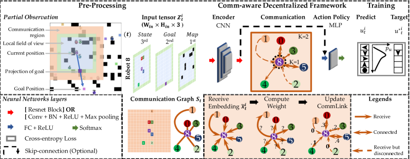
Figure 1: Our proposed decentralized framework. (i) illustrates how we process the partial observations of each robot into input tensor ${\mathbf{Z}}_{t}^{i}$, and how we construct the dynamic communication network. (ii) demonstrates the processing pipeline consisting of a feature extractor, a graph convolution module, and an Multi-layer Perceptron (MLP). The optional skip connection represents the bottleneck structure discussed in Sec. VI. (iii) visualizes how our model gathers features, computes attention weights by a key-query-like attention mechanism (sandy brown), and selectively aggregates useful features.

V-A Properties of MAGAT

Given our task formulation, the topology of the communication graph ${\mathcal{G}}_{t}$ changes with time. Other robots can enter and leave the communication range of the robot at any time, leading to a frequent change of the graph topology. Therefore, it is necessary to discuss whether our trained MAGAT performs graph convolutions consistently regardless of agent permutation and time shift.

V-A1 Permutation Equivariance

MAGAT must satisfy permutation equivariance, which ensures that the trained MAGAT is resistant to the change of robot orders and always gives the same convolution results regardless of how we swap the order indices when constructing the dynamic graph.

We first define a permutation $\pi$ as swapping the indices of robots. The permutation results in a swapped order of features:

$$\pi({\mathbf{X}}_{t})=\begin{bmatrix}({\tilde{\mathbf{x}}}_{t}^{\pi^{-1}(1)})^{\mathsf{T}}\\ \vdots\\ ({\tilde{\mathbf{x}}}_{t}^{\pi^{-1}(N)})^{\mathsf{T}}\end{bmatrix}~{}.$$ (10)

A permutation matrix ${\mathbf{P}}_{\pi}\in\{0,1\}^{N\times N}$ is thus defined to swap graph features directly:

$$\begin{bmatrix}{\mathbf{P}}_{\pi}{\mathbf{X}}_{t}\end{bmatrix}_{ij}=\begin{bmatrix}{\mathbf{X}}_{t}\end{bmatrix}_{\pi^{-1}(i)j}~{}.$$ (11)

Lemma 1.

Given a permutation $\pi$, its corresponding permutation matrix $P_{\pi}$, and the convolution operation ${\mathcal{A}}_{G}$ of GNN defined in Eq. 3, the following equation can be derived from [21]:

$${\mathbf{P}}_{\pi}{\mathcal{A}}_{G}({\mathbf{X}}_{t};{\mathbf{S}}_{t})={\mathcal{A}}_{G}({\mathbf{P}}_{\pi}{\mathbf{X}}_{t};{\mathbf{P}}_{\pi}{\mathbf{S}}_{t})~{}.$$ (12)

Proposition 1 (Permutation Equivariance of MAGAT).

For any permutation $\pi$, its corresponding permutation matrix $P_{\pi}$ and the convolution operation ${\mathcal{A}}_{F}$ of MAGAT defined in Eq. 5, the following equation holds:

$${\mathbf{P}}_{\pi}{\mathcal{A}}_{F}({\mathbf{X}}_{t};{\mathbf{S}}_{t})={\mathcal{A}}_{F}({\mathbf{P}}_{\pi}{\mathbf{X}}_{t};{\mathbf{P}}_{\pi}{\mathbf{S}}_{t})~{}.$$ (13)

Proof.

Recall that Eq. 7 implies that attention $e_{ij}$ is only determined by the node features ${\tilde{\mathbf{x}}}_{t}^{i}$ and ${\tilde{\mathbf{x}}}_{t}^{j}$. Thus, using the permutation operation defined in Eq. 11, we can permute the robot indices in the attention matrix as follows:

$$\begin{bmatrix}{\mathbf{P}}_{\pi}{\mathbf{E}}\end{bmatrix}_{ij}=\mathrm{softmax}(e_{\pi^{-1}(i)j})=\begin{bmatrix}{\mathbf{E}}\end{bmatrix}_{\pi^{-1}(i)j}~{}.$$ (14)

This means that the swap of robots will only permute the attention matrix in a similar way with graph features. Then we can show that in our MAGAT:

$${\mathcal{A}}_{F}({\mathbf{P}}_{\pi}{\mathbf{X}}_{t};{\mathbf{P}}_{\pi}{\mathbf{S}}_{t})= \sum_{k=0}^{K-1}({\mathbf{P}}_{\pi}{\mathbf{E}}\odot{\mathbf{P}}_{\pi}{\mathbf{S}}_{t})^{k}{\mathbf{P}}_{\pi}{\mathbf{X}}_{t}{\mathbf{A}}_{k}$$ (15)

$$= \sum_{k=0}^{K-1}({\mathbf{P}}_{\pi}({\mathbf{E}}\odot{\mathbf{S}}_{t}))^{k}{\mathbf{P}}_{\pi}{\mathbf{X}}_{t}{\mathbf{A}}_{k}$$

$$= {\mathbf{P}}_{\pi}\sum_{k=0}^{K-1}({\mathbf{E}}\odot{\mathbf{S}}_{t})^{k}{\mathbf{X}}_{t}{\mathbf{A}}_{k}~{}.$$

The last step uses the permutation equivariance property of GNN from Lemma 1, taking ${\mathbf{E}}\odot{\mathbf{S}}_{t}$ as a whole to replace the ${\mathbf{S}}_{t}$ in GNN. ∎

V-A2 Time Invariance

MAGAT must satisfy the time invariance criterion, in order to generate consistent output when the same situation appears again in a different step of the simulation.

Proposition 2 (Time Invariance of MAGAT).

Given $t_{1}\not=t_{2}$, ${\mathbf{X}}_{t_{1}}={\mathbf{X}}_{t_{2}}$ and ${\mathbf{S}}_{t_{1}}={\mathbf{S}}_{t_{2}}$, and the convolution operation ${\mathcal{A}}_{F}$ of MAGAT in Eq. 5, the following equation holds:

$${\mathcal{A}}_{F}({\mathbf{X}}_{t_{1}};{\mathbf{S}}_{t_{1}})={\mathcal{A}}_{F}({\mathbf{X}}_{t_{2}};{\mathbf{S}}_{t_{2}})~{}.$$ (16)

Proof.

This criterion is satisfied intrinsically by our imitation strategy (Sec. VI-D): the decentralized framework is trained to enable the robot to predict consistent action ${\mathbf{U}}_{t}^{*i}$ only with respect to input tensor ${\mathbf{Z}}_{t}^{i}$ and communication network ${\mathbf{S}}_{t}$ regardless of the time instant $t$. ∎

VI Architecture

In this section, we start by introducing the dataset creation (Sec. VI-A), and move on to show how we process the observations (Sec. VI-B) and the detailed architecture of our proposed model (Sec. VI-C). Finally, we present the training process, which is enhanced by an online expert (Sec. VI-D).

VI-A Dataset Creation

We generate grid worlds of size $W\times H$ and randomly place static obstacles of a given density. For each grid world, we generate cases where the start positions and goal positions are not duplicated. We filter duplicates and then call an expert algorithm to compute solutions. Invalid cases (those who do not have a solution, e.g., robots are trapped by static obstacles) are removed at this stage. Towards this end, we run a coupled centralized expert algorithm: Enhanced Conflict-Based Search (ECBS)  with optimality bound $1.1$ [2]. This expert algorithm computes our ‘ground-truth paths’ (the sequence of actions for individual robots) for a given initial configuration. Our data set comprises $30{,}000$ cases for any given map size and number of robots. This data is divided into a training set ($70\%$), a validation set ($15\%$), and a testing set ($15\%$). The three sets do not overlap with each other.

VI-B Processing Observations

Limited by the local FOV, each robot perceives an observation and processes it to be ${\mathbf{Z}}_{t}^{i}\in{\mathbb{R}}^{3\times W_{\mathrm{in}}\times H_{\mathrm{in}}}$, which consists of three channels, representing static obstacles, robots, and goal respectively. Note that, $W_{\mathrm{in}}=W_{\mathrm{FOV}}+2$ and likewise for $H_{\mathrm{in}}$: when the goal is outside the FOV, we mark a point on the edge of the goal channel of ${\mathbf{Z}}_{t}^{i}$ to indicate the direction of the target (Fig. 1). This ensures that each robot has only the direction of the target when the goal is outside the FOV.

VI-C Network Architecture

CNN-based Perception. Compared to our previous work [4], we upgrade the CNN module with ResNet blocks as follows: we implement a feature extractor with 3 stacked residual blocks. Different from the conventional Conv2d-BatchNorm2d-ReLU-MaxPool2d structure, there is a skip connection in each block joining the features before and after the block together. This type of residual connection has been widely used in feature extraction work, and it has been shown to be beneficial to reducing overfitting and improving performance [22].

Graph-based Communication. Each individual robot carries a local copy of the graph convolution layers and communicates its compressed observation vector ${\tilde{\mathbf{x}}}_{t}^{i}$ with neighboring robots within its communication radius $r_{\mathrm{COMM}}$. The resulting fused feature is then passed to the next stage for selecting the action primitive, leading to a localized decision-making scheme.

In the graph convolution architecture, we explore several models with two main types of graph convolution layers: GNN and MAGAT. To better demonstrate the improvements that MAGAT can make in our task, we compare each MAGAT model with the corresponding GNN model with the same configuration except the graph convolution layers. These models are defined in the form of “[Config_Label]-[Type]-[Num_Features]”:

1. Config_Label: can be GNN or MAGAT. It refers to the graph convolution layer used in this model.

2. Type: “F” refers to normal CNN-MLP-GraphConvLayer
   -MLP-Action pipeline, while “B” refers to a bottleneck structure (Fig. 1), which concatenates the feature before the graph convolution layers with those processed features after the graph convolution layers. This bottleneck structure augments the features after communication with the features extracted by the robot itself.

3. Num_features: the dimensions of features that engage in communication. In this paper, we experiment with $128$, $64$, $32$, and $16$.

To demonstrate the information reduction in communication, we constrain the dimensions of extracted features from the CNN module to be 128, and further reduce the dimensionality using an additional MLP layer. The number of input observations $F$ and output observations $G$ are the same and set to Num_features. This effectively reduces the dimensions of features that can be shared by the communication network.

In this paper, we focus on $L=1$ (one layer of graph convolution) and $K=2$ (one-hop communication). Each robot is required to send all its extracted features and receive information from neighboring robots only once. With the help of our mechanism, the robot is able to direct its attention toward specific communication links, based on the relative importance of the information contained in the messages it is receiving from neighboring robots.

Action Policy. In the last stage, an MLP followed by a softmax function is used to decode the aggregated features resulting from the communication process into the five motion primitives (up, down, left, right, and idle). During the simulation, the action ${\tilde{\mathbf{u}}}_{t}^{i}$ taken by robot $i$ is predicted by a stochastic action policy based on the probability distribution over motion primitives (weighted sampling). We deployed collision shielding in [4] to ensure collision-free paths. Compared to our previous framework [4], we change the action policy used in the simulations of the validation process from a softmax function (deterministic policy) to weighted sampling (stochastic policy), as using a consistent action policy for validation and test can better indicate which models to select after training.

VI-D Training and Online Expert

After training cases are generated and the optimal trajectory of each robot is computed by a centralized controller, the model is trained by the trajectory data, such that it imitates the actions and behaviors of the “expert”. We train the model with the pair collection ${\mathcal{T}}=\{({\mathbf{Z}}_{t}^{i},{\mathbf{U}}_{t}^{*i})\}_{i=1,...,N_{case},t=1,...,T_{max}^{i}}$, where ${\mathbf{Z}}_{t}^{i}$ is the processed observation (Sec. VI-B) at time $t$ of case $i$, while ${\mathbf{U}}_{t}^{*i}$ is the expert action at this situation consisting of ${\tilde{\mathbf{u}}}_{t}^{*i}$ taken by robot $i=1,...,N_{robot}$. Note that $N_{case}$ and $T_{max}^{i}$ are the total number of cases and the total steps of case $i$, respectively. Thus, our training does not involve time sequence information, requiring the model to learn “instant” reactions based on observations at any given time $t$.

To further enhance model learning, we deploy the Online Expert proposed in our previous work [4] right after every validation process: We select $n_{OE}$ cases randomly from the training set and run the simulation. New solutions are generated for the failed cases using the ECBS solver. These new solutions become new cases and are appended to the training set: ${\mathcal{T}}_{new}={\mathcal{T}}\cup\{({\mathbf{Z}}_{t}^{i},{\mathbf{U}}_{t}^{*i})\}_{i=1,...,n_{OE},t=1,...,T_{max}^{i}}$.

Therefore, our training objective is to obtain a classifier ${\mathcal{F}}$ with trainable parameters $\theta$ given the training dataset ${\mathcal{T}}$ that is gradually augmented. $\mathcal{L}$ is the loss function.

$$\hat{\theta}=\operatornamewithlimits{argmin}_{\theta}\sum_{({\mathbf{Z}}_{t}^{i},{\mathbf{U}}_{t}^{*i})\in{\mathcal{T}}}{\mathcal{L}({\mathbf{U}}_{t}^{\ast},{\mathcal{F}}({\mathbf{Z}}_{t}^{i},{\mathcal{G}}_{t}({\mathbf{Z}}_{t}^{i})))}~{}.$$ (17)

Recall that ${\mathcal{G}}_{t}$ is the status of the communication network at time $t$ depending on current situation ${\mathbf{Z}}_{t}^{i}$.

VII Experiments

In this section, we firstly introduce the metrics we use in the evaluation (Sec. VII-A), and then provide details of the experimental setup (Sec. VII-B). We then move on to introduce the map sets we use in the experiments (Sec. VII-C) and the baselines against which we compare our proposed methods (Sec. VII-D). Finally, we present and discuss our experimental results (Sec. VII-E).

VII-A Metrics

1) Success Rate ($\alpha$) $=n_{\mathrm{success}}/n$, is the proportion of successful cases over the total number of tested cases $n$. A case is considered successful (complete) when all robots reach their goals prior to exceeding the maximum allowed steps. In our case, the max allowed step (i.e., maximum makespan) is normally set to $T_{\max}=3T_{\mathrm{MP}^{*}}$, where $T_{\mathrm{MP}^{*}}$ is the makespan (the time period from the first robot moves to the last robot arrives its goal) of the expert solution.

2) Flowtime Increase ($\delta_{\mathrm{FT}}$) $=(\mathrm{FT}-\mathrm{FT}^{*})/\mathrm{FT}^{*}$, measures the difference between the sum of the executed path lengths ($\mathrm{FT}$) and that of the expert (target) path ($\mathrm{FT}^{*}$). We set the length of the predicted path $T^{i}=T_{\max}=3T_{\mathrm{MP}^{*}}$, if the robot $i$ does not reach its goal. This contributes a penalty to the total flowtime if a robot fails to reach its goal.

VII-B Experimental Setup

Our simulations were conducted using the Cambridge High-Performance Computing Wilkes2-GPU NVIDIA P100 cluster with Intel(R) Xeon(R) CPU E5-2650 v4 (2.20GHz). We used the Adam optimizer with momentum $0.9$. The learning rate $\gamma$ was scheduled to decay from $10^{-3}$ to $10^{-6}$ within 300 epochs, using cosine annealing. We set the batch size to $64$, and L2 regularization to $10^{-5}$. The online expert was deployed every $C=4$ epochs on $n_{\mathrm{OE}}=500$ randomly selected cases from the training set. Validation was carried out every 4 epochs with 1000 cases that were exclusive of the training/test set.

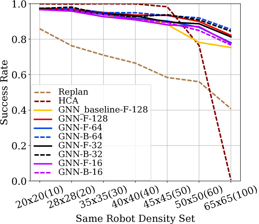
(a) Success rate ($\alpha$) at GNN

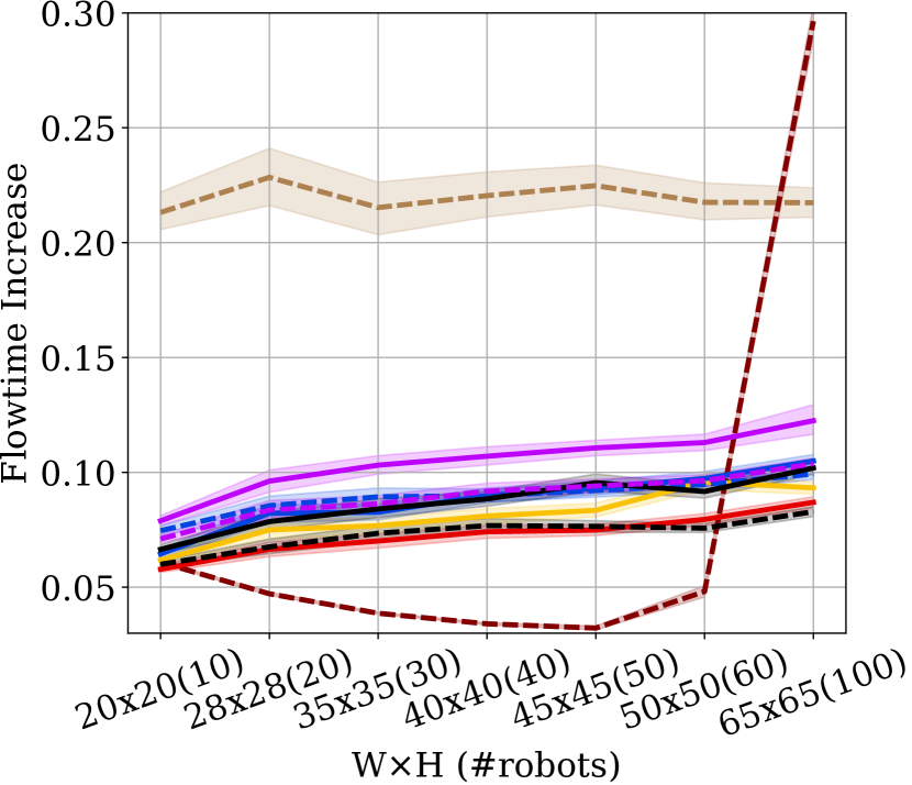
(b) Flowtime increase ($\delta_{\mathrm{FT}}$) at GNN

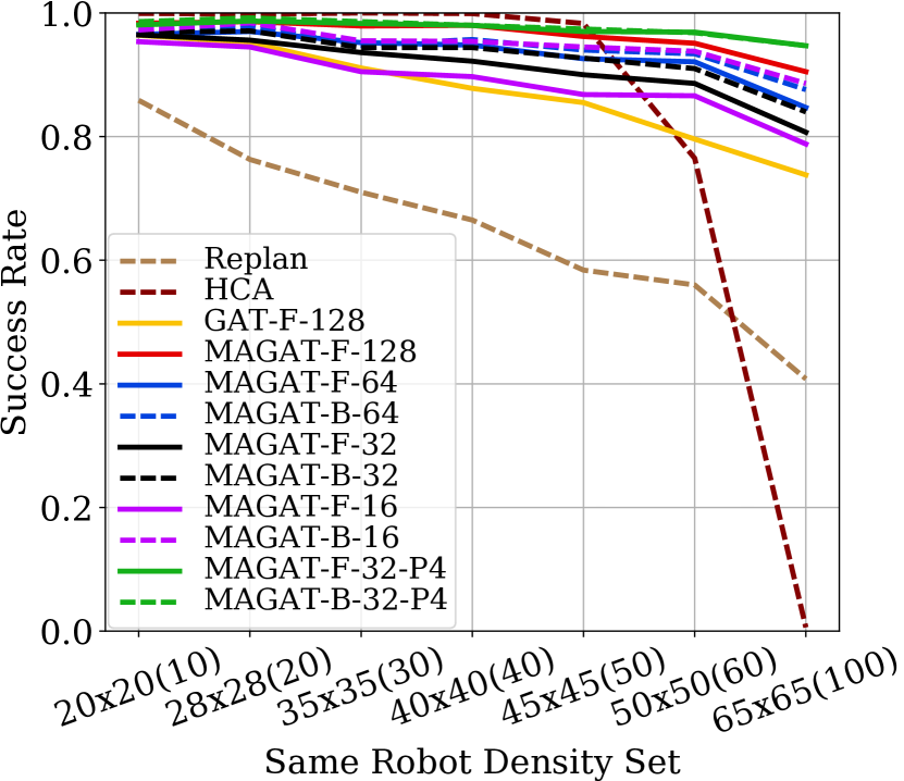
(c) Success rate ($\alpha$) at MAGAT

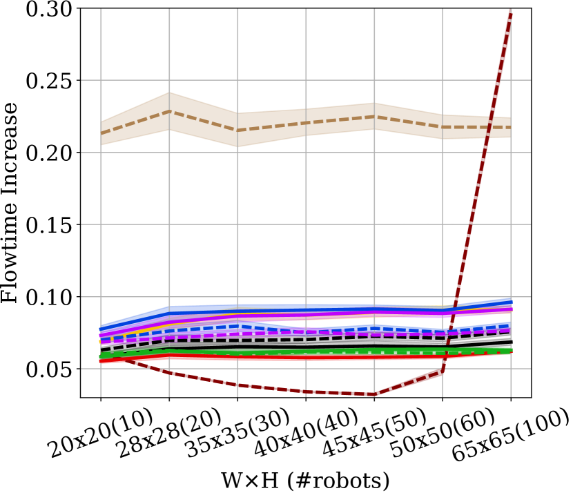
(d) Flowtime increase ($\delta_{\mathrm{FT}}$) at MAGAT

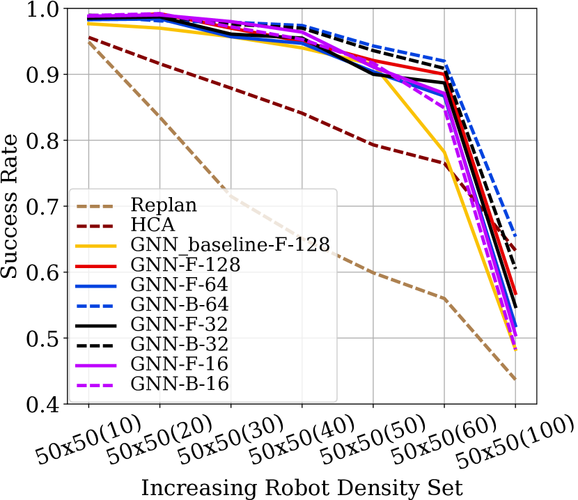
(e) Success rate ($\alpha$) at GNN

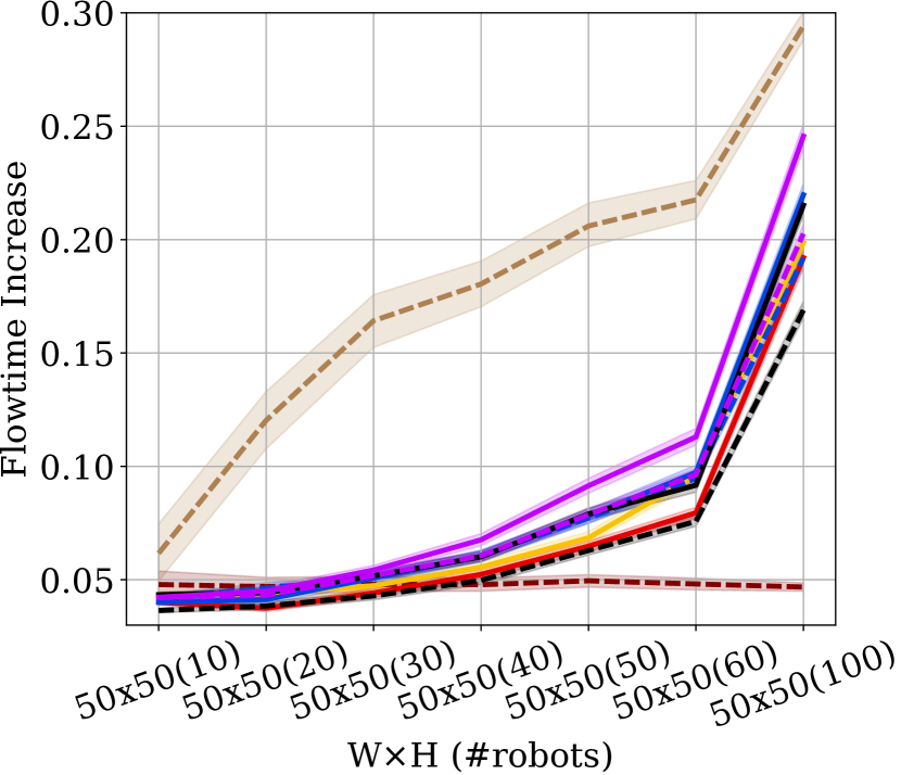
(f) Flowtime increase ($\delta_{\mathrm{FT}}$) at GNN

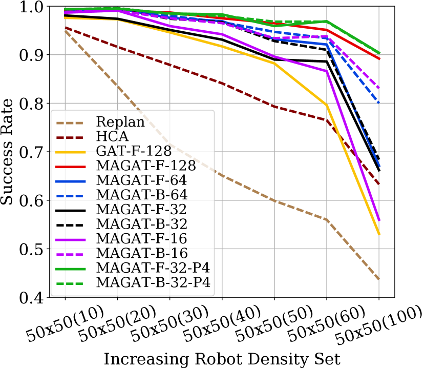
(g) Success rate ($\alpha$) at MAGAT

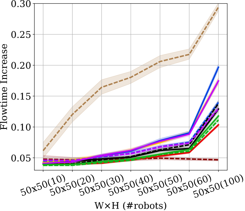
(h) Flowtime increase ($\delta_{\mathrm{FT}}$) at MAGAT

Figure 2: The success rate ($\alpha$) and flowtime increase ($\delta_{\mathrm{FT}}$) against the change of environment setup. Here we present the results of GNN models on the left two columns and MAGAT models on the right; we include HCA and Replan as baselines. The first row is for “Same Robot Density Set”, while the second is for “Increasing Robot Density Set”. These figures show the effects of reducing bandwidth or using bottleneck structure. In the legend ([Graph_Layer_Name]-[Type]-[Num_Features]), Graph_Layeer_Name are GNN or MAGAT, while Type - “F” and solid line refer to normal CNN-MLP-GNN/MAGAT-MLP-Action pipeline, and “B” and dashed line refer to a bottleneck structure. [Num_Features] includes 128 (red), 64 (blue), 32 (black), and 16 (purple).

VII-C Scenarios

To better compare the generalization capability, we prepare training/valid/test datasets according to Table I. We train and validate our models with 20$\times$20 maps and 10 robots, and then test on all scenarios shown in Table I.

In practice, robot density ($\rho_{robot}$), simply computed by $\frac{n_{robot}}{W\times H}$, is an effective metric measuring how crowded a scenario is. Note that the obstacle densities in all scenarios in Table I, II are $10\%$. We test model generalization ability with two sets of maps. One is “Same Robot Density Set”, with all scenarios having the same robot density. Using this map set, we are able to test the generalization of the models on the maps with similar robot density to the training sets. On the other hand, “Increasing Robot Density Set” is a set with increasing robot density, but the map size remains the same. With this map set, we gradually increase the crowdedness, leading to our evaluation of how our model can perform under sparser or more congested environments.

Additionally, we prepare a super-large-scale test set, which has over 500 robots and a very large map size (Table II). There are 50 test cases in each large-scale scenario.

TABLE I: Two major map sets for generalization test. Training scenario 20$\times$20 with 10 robots has 30000 cases, partitioned into 70% training set, 15% validation set, and 15% test set. Other scenarios have 1000 testing cases for the generalization test.

Same Robot Density Set		Increasing Robot Density Set
Map ($n_{robot}$)	Robot Density	Map ($n_{robot}$)	Robot Density
20x20 (10)	0.025	50x50 (10)	0.004
28x28 (20)	0.025	50x50 (20)	0.008
35x35 (30)	0.025	50x50 (30)	0.012
40x40 (40)	0.025	50x50 (40)	0.016
45x45 (50)	0.025	50x50 (50)	0.02
50x50 (60)	0.025	50x50 (60)	0.024
65x65 (100)	0.025	50x50 (100)	0.04

TABLE II: Large Scale Map Set. The expert computation time in the $3rd$ column is the time cost of using the ECBS solver with an optimality bound $5$ to solve the case on a high-performance CPU core. The computation time (successful cases) of our proposed model MAGAT-B-32-P4 in the same machine is reported in the $4th$ column. Statistics in bold highlight the significant reduction in the computation time of our model.

Map ($n_{robot}$)	$\rho_{robot}$	Expert time cost (s)	Time cost (s) (std.)
200x200 (500)	0.0125	~3,000 - 4,000	510.1 (135.0)
200x200 (1000)	0.025	~33,000. - 35,000	1286.8 (368.0)
100x100 (500)	0.05	~1,100 - 1,200	279.92 (83.0)

VII-D Baselines

We introduce two models and two non-learning based methods as our baselines.

1. GNN_baseline-F-128: The GNN framework we proposed in previous work [4]. Since then, we have upgraded the CNN module for feature extraction and the action policy in the validation process (details in Sec. VI-C). Therefore, it represents a good baseline demonstrating the basic improvement that we make to the framework.

2. GAT-F-128: The framework is the same as our MAGAT, but instead of our attention mechanism (Eq. 7), the mechanism of GAT [16] (introduced in Eq. 9) is used.

3. HCA: A simple domain abstraction with a heuristic to improve the performance of centralized multi-robot path planning [23].

4. Replan: Global Re-planning (Replan) is an interaction-aware path planning method [11]. If the robot encounters a conflict, the A* method is used to find an alternative path from the current cell to the goal cell, considering all other robots as obstacles.

VII-E Results

All the results shown in this section are obtained by training on a dataset composed of 20$\times$20 maps with $10$ robots (21000 training cases).

VII-E1 Comparison with baselines

As shown in Fig. 2, our GNN-F-128 and MAGAT-F-128 both outperform their baseline models, GNN_baseline-F-128 and GAT-F-128 respectively. For instance, at “Same Robot Density Set”, GNN-F-128 (solid red line) performs slightly better than its baseline GNN_baseline-F-128 (solid yellow line) when the map size is lower than 40. The gap becomes significant ($>5\%$ in success rate) as we scale the testing set beyond $40\times 40$ with 40 robots. Similar results are observed at “Increasing Robot Density Set”, and these demonstrate that our upgrades on the CNN module and the action policy are useful. Under both map sets, MAGAT-F-128 (solid red line) outperforms GAT-F-128 (solid yellow line) in both success rate and flowtime increase significantly, whose performance is only close to that of MAGAT-F-16 (solid purple line). The underlying reasons for this are discussed in Sec. V. HCA (light brown) performs quite well with a high success rate and small flowtime increase when cases are simple, but its performance suddenly drops down starting from 40 robots; it cannot find a solution for 100 robots. The success rate (completeness) of Replan (dark red) is generally low compared with our methods, with a higher flowtime increase.

VII-E2 Effect of reducing the information shared among robots

We further experiment with limited communication bandwidth, i.e., limiting the size of the shared features from 128 (red), 64 (blue), 32 (black) to 16 (purple), where the full communication bandwidth is set as 128. In Fig. 2, we show the success rate and flowtime increase of GNN and MAGAT family, respectively. With both GNN and MAGAT configurations, the performance will decrease as we reduce the size of shared features. E.g., as the shared features decrease from 128, 64, 32 to 16, the success rate of MAGAT models at 65$\times$65 with 100 robots drop from 91%, 85%, 81% to 78% respectively. Yet, the drop of MAGAT is less pronounced than with GNN, where the performance of GNN models decreases from 83%, 78%, 82% to 77% respectively, as the shared features reduce from 128, 64, 32 to 16.

VII-E3 Generalization under different robot densities

Recall that the “Same Robot Density Set” has the same robot density for all its cases. Generalizability is an essential factor to evaluate a machine learning model in real-world applications. The mobility of multi-robot systems naturally leads to time-varying communication topologies. Thus, “Increasing Robot Density Set” allows us to better evaluate the model’s flexibility from sparse to more crowded situations. As shown in the Fig. 2(e), Fig. 2(f), Fig. 2(g) and Fig. 2(h), most MAGAT models can maintain the success rate above 92% and the flowtime increase lower than 10% even as we increase robot number from 10 to 60 on the same map size (50$\times$50), which demonstrates their good adaptation to different crowdedness.

VII-E4 Effect of bottleneck architecture

Fig. 2 also explores the performance of the skip-connected bottleneck structure with GNN and MAGAT. In real-world applications, the communication bandwidth is usually limited which yields the need to have fewer features being shared but performance maintained. For fair comparisons, models are compared to their “baseline” models, for example, comparing GNN-F-64 (solid blue line) and GNN-B-64 (dashed blue line) because they have the same size of features shared across the communication network. With the bottleneck setting, GNN-B-64 outperforms GNN-F-64 by around 8% in success rate under the scenario of $65\times 65$ maps with 100 robots (Fig. 2(a)). In Fig. 2(c), even though the performance of MAGAT drops dramatically from 90% (MAGAT-F-128, solid red line) to around 78% (MAGAT-F-16, solid purple line) in success rate at 65$\times$65 maps with 100 robots, the bottleneck structure retains its performance such that it is comparable with MAGAT-F-128. This gives the insight that the good generalization ability of MAGAT rests on a sufficient size of the shared features, but it can be preserved by introducing the bottleneck structure. We can conclude that though GNN models do not significantly benefit from a bottleneck structure, this structure helps MAGAT models maintain generalization performance significantly.

VII-E5 Effect of multi-head attention

We also evaluate MAGAT-F-32 (solid blue line) and MAGAT-B-32 (dashed
blue line) on their multi-head versions MAGAT-F-32-P4 
(solid green line) and MAGAT-B-32-P4 (dashed green line). Note that $P$ = $4$ parallel MAGAT convolution layers allow larger model capacities, and individual heads can learn to focus on different representation subspaces of the node features [19]. For these two models, as there are $P\times F=4\times 32=128$ features being shared, the total bandwidth (or the size of shared features) is the same as MAGAT-F-128, leading to a fair comparison. In Fig. 2(c), Fig. 2(d), Fig. 2(g) and Fig. 2(h), the multi-head version demonstrates better performance across all the tests regardless of the robot density and map size. Both multi-head models achieve $95\%$ success rate in 50$\times$50, 100 robots, and their results for flowtime increase under “Same Robot Density Set” remain at low values ($\delta_{\mathrm{FT}}$ < $0.065$) even with increasing robot numbers.

VII-E6 Super-large-scale generalization

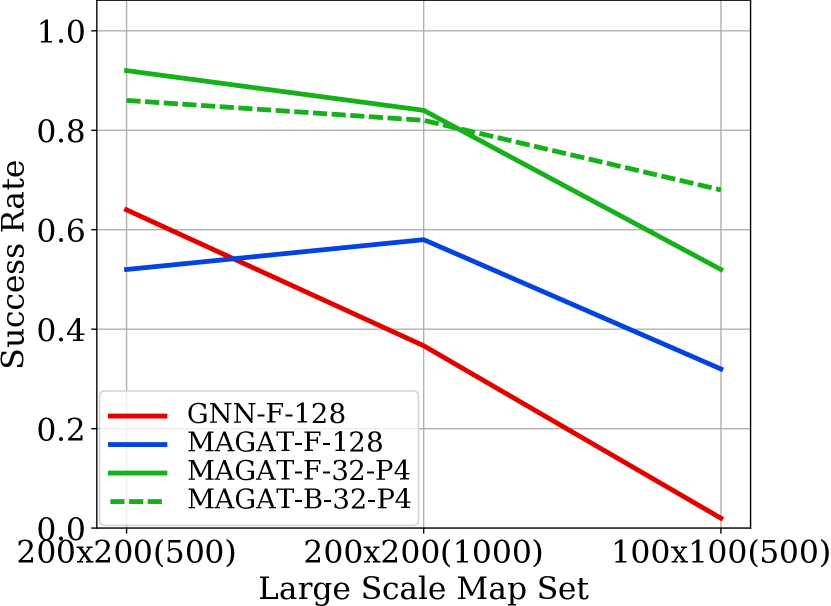
(a) Success rate

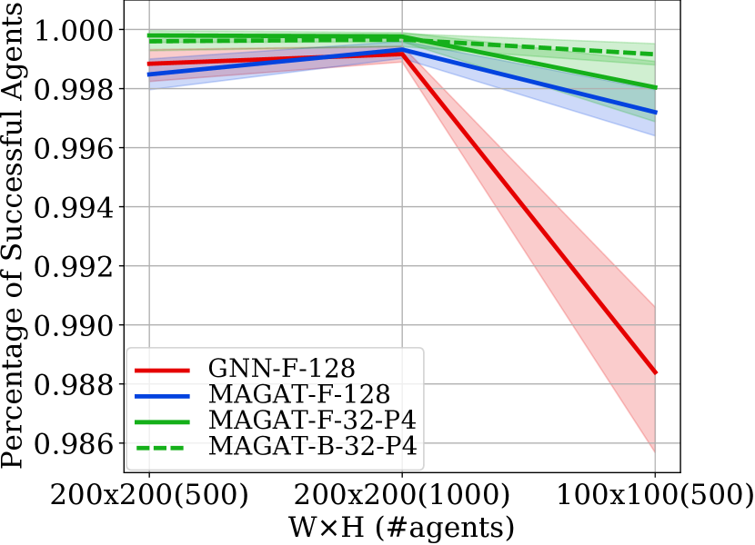
(b) $p_{\mathrm{robot}}$

Figure 3: Generalization test on Large Scale Map Set. a) shows the success rate. b) shows the percentage of successful robots ($p_{\mathrm{rg}}=\frac{n_{\mathrm{robots\,reach\,goal}}}{n_{\mathrm{robot}}}$), indicating that those model with low success rates can still successfully navigated most of the robots to their goals.

We also test GNN and MAGAT with the large-scale map set, which consists of harder cases that set high requirements for such a model that is trained only on 20$\times$20 with 10 robots. Table II shows that, with such a large amount of robots ($1000$ robots), traditional expert algorithms are not capable of solving the problem within an acceptable time. Given the decentralized nature of our framework, the trained models are efficient in the sense that their computation is distributed among the robots, demanding only communication exchanges with neighboring robots. Even though MAGAT-B-32-P4 is only trained by the expert solutions of 20$\times$20 with $10$ robots, it can obtain a success rate above $80\%$ at $200\times 200$ map with $1000$ robots, with only $\frac{1}{30}$ of the computation time taken by the centralized coupled expert (Table II). Fig. 3(b) demonstrated that in all cases, at least $98.6\%$ robots have already reached their goals. At 100$\times$100 map with $500$ robots, MAGAT models successfully achieve at least $p_{\mathrm{rg}}$ = $99.6\%$ robot navigation, but for GNN this number drops down to $98.6\%$.

VII-E7 Summary

In conclusion, we note that MAGAT has very promising potential in learning a generalizable and flexible dynamic decision-making policy. In general, even in some cases where MAGAT and GNN have a similar success rate, MAGAT reduces the flowtime further, leading to more robots achieving their goals and more optimal paths. MAGAT also shows its ability to learn more general knowledge about path finding, which is supported by the fact that it can achieve high performance in large-scale and challenging cases even though it is trained in very simple cases. We also demonstrate that the multi-head attention of MAGAT can improve performance. The trained model achieves a 47% improvement over the benchmark success rate in the $200\times 200$ map with $1000$ robots, where the testing instances are $\times$100 larger than the training instances.

VIII Conclusion and Future Work

Conclusion. We conduct pioneering research that utilizes a decentralized message-aware graph attention network to solve the multi-agent path planning problem. We formulate our problem as a sequential decision-making problem, and we incorporate an attention mechanism to enable the GNN to selectively aggregate message features. We prove theoretically and empirically that MAGAT is capable of dealing with dynamic communication graphs, and that it demonstrates good generalizability on unseen environment settings and strong scalability on super large-scale cases while we train the model with only very simple cases. We also show that the skip-connected bottleneck structure is a way to maintain model performance while reducing the information being shared. This feature enables MAGAT to achieve good performance while transmitting less data, leading to significant value in practice and applications. The results demonstrate that the multi-head attention is beneficial to MAGAT models, where individual heads can learn to focus on different representation subspaces of the node features [19].

In the future, we will evaluate our framework in different map types, including maze and warehouse-like maps. We are interested in upgrading it from the discrete world to a continuous one. Experiments with real physical robots are already on our agenda.

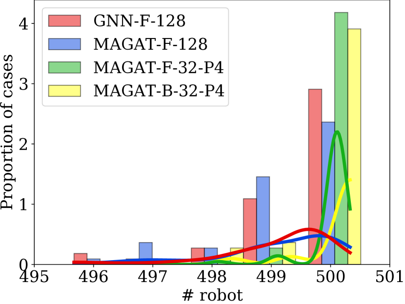
(a) $200\times 200$(500)

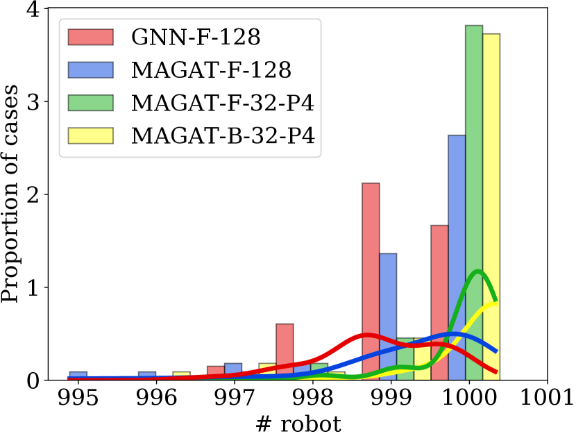
(b) $200\times 200$(1000)

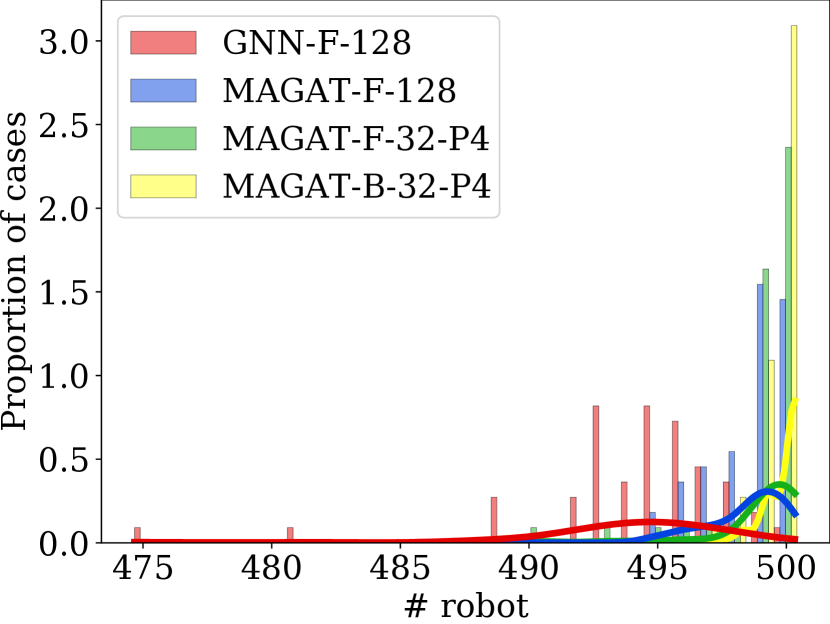
(c) $100\times 100$(500)

Figure 4: Histogram of proportion of cases distributed over the number of robots reaching their goal; GNN-F-128(red), MAGAT-F-128(blue), MAGAT-F-32-P4(green) and MAGAT-B-32-P4(yellow), are trained on $20\times 20$ with 10 robots and tested on $200\times 200$ with 500, 1000 robots, and $100\times 100$ with 500 robots.

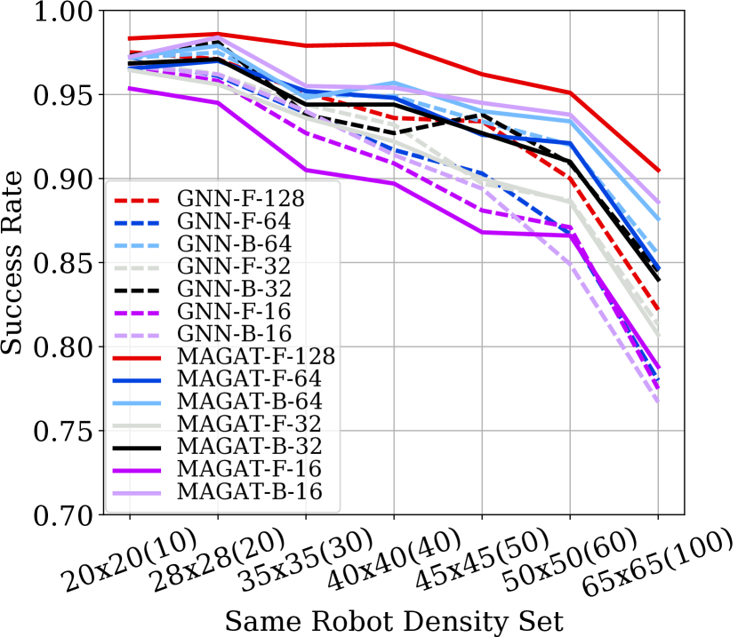
(a) Success rate $\alpha$

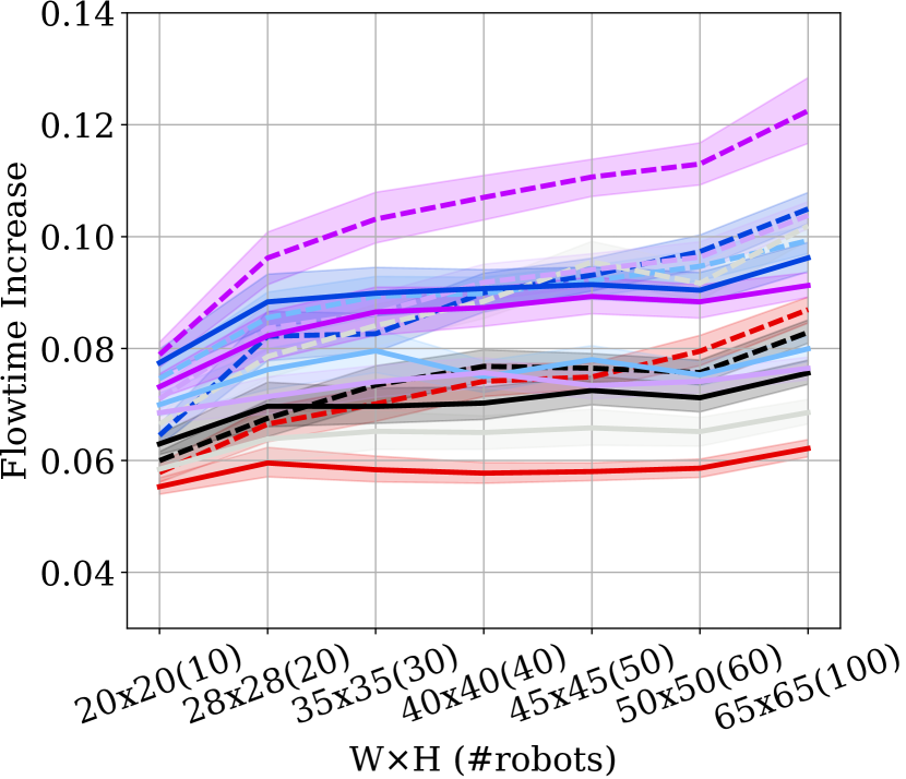
(b) Flowtime increase $\delta_{\mathrm{FT}}$

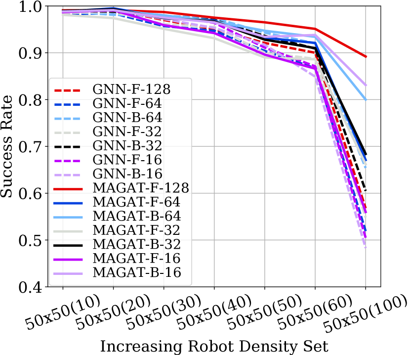
(c) Success rate $\alpha$

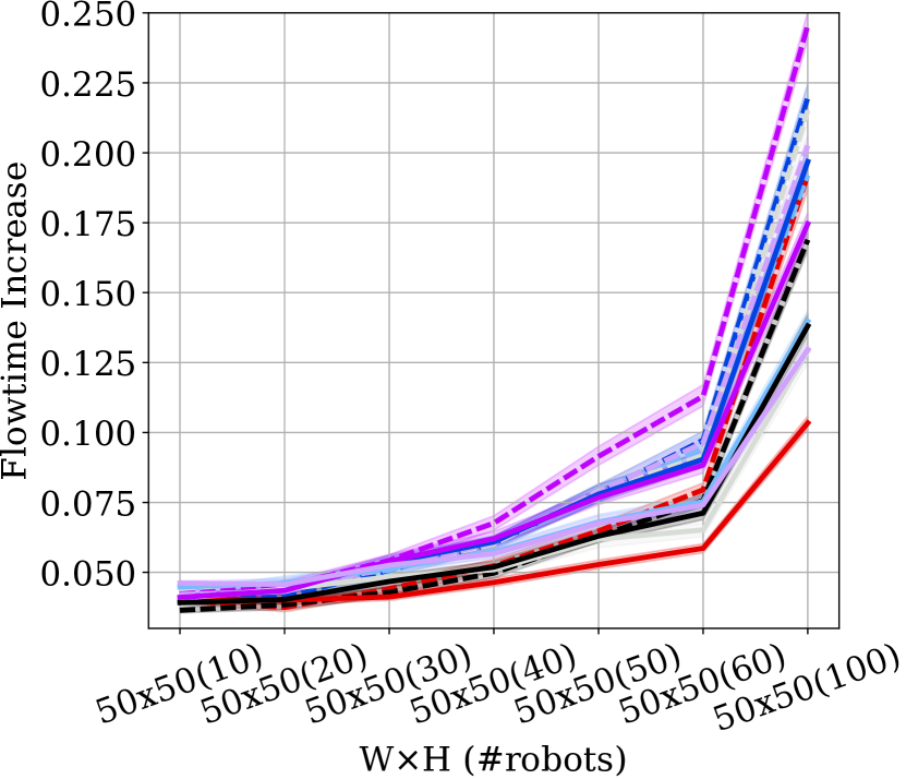
(d) Flowtime increase $\delta_{\mathrm{FT}}$

Figure 5: The success rate ($\alpha$) and flowtime increase ($\delta_{\mathrm{FT}}$) against the change of environment setup. Here we present some selected results of GNN and MAGAT in both “Same Robot Density Set” (Panel a and b) and “Increasing Robot Density Set” (Panel c and d). The results demonstrated that MAGAT is able to generalize better to more extreme unseen cases. In the legend ([Graph_Layer_Name]-[Type]-[Num_Features]), Graph_Layeer_Name are GNN (dashed line) or MAGAT (solid line), while Type - “F” refer to normal CNN-MLP-GNN/MAGAT-MLP-Action pipeline, and “B” refer to a bottleneck structure. [Num_Features] includes 128 (red), 64 (blue), 32 (black), 16 (purple).

References

- [1] J. Van den Berg, M. Lin, and D. Manocha, “Reciprocal velocity obstacles for real-time multi-agent navigation,” in IEEE International Conference on Robotics and Automation, 2008, pp. 1928–1935.
- [2] M. Barer, G. Sharon, R. Stern, and A. Felner, “Suboptimal variants of the conflict-based search algorithm for the multi-agent pathfinding problem,” in European Conference on Artificial Intelligence, 2014, pp. 961–962.
- [3] G. Sartoretti, J. Kerr, Y. Shi, G. Wagner, T. Kumar, S. Koenig, and H. Choset, “Primal: Pathfinding via reinforcement and imitation multi-agent learning,” IEEE Robotics and Automation Letters, vol. 4, no. 3, pp. 2378–2385, 2019.
- [4] Q. Li, F. Gama, A. Ribeiro, and A. Prorok, “Graph neural networks for decentralized multi-robot path planning,” in IEEE/RSJ International Conference on Intelligent Robots and Systems, 2020, pp. 11 785–11 792.
- [5] J. Enright and P. R. Wurman, “Optimization and coordinated autonomy in mobile fulfillment systems.” in AAAI Workshop on Automated Action Planning for Autonomous Mobile Robots, 2011, pp. 33–38.
- [6] A. Prorok and V. Kumar, “Privacy-preserving vehicle assignment for mobility-on-demand systems,” in IEEE/RSJ International Conference on Intelligent Robots and Systems, 2017, pp. 1869–1876.
- [7] J. P. van den Berg and M. H. Overmars, “Prioritized motion planning for multiple robots,” in IEEE/RSJ International Conference on Intelligent Robots and Systems, 2005, pp. 430–435.
- [8] M. Fowler, P. Tokekar, T. C. Clancy, and R. K. Williams, “Constrained-action pomdps for multi-agent intelligent knowledge distribution,” in IEEE International Conference on Robotics and Automation, 2018, pp. 3701–3708.
- [9] G. Best, M. Forrai, R. R. Mettu, and R. Fitch, “Planning-aware communication for decentralised multi-robot coordination,” in IEEE International Conference on Robotics and Automation, 2018, pp. 1050–1057.
- [10] J. Tobin, R. Fong, A. Ray, J. Schneider, W. Zaremba, and P. Abbeel, “Domain randomization for transferring deep neural networks from simulation to the real world,” in IEEE/RSJ International Conference on Intelligent Robots and Systems, 2017, pp. 23–30.
- [11] B. Wang, Z. Liu, Q. Li, and A. Prorok, “Mobile robot path planning in dynamic environments through globally guided reinforcement learning,” IEEE Robotics and Automation Letters, vol. 5, no. 4, pp. 6932–6939, 2020.
- [12] J. Foerster, I. A. Assael, N. De Freitas, and S. Whiteson, “Learning to communicate with deep multi-agent reinforcement learning,” in Advances in Neural Information Processing Systems, 2016, pp. 2137–2145.
- [13] B. Freed, R. James, G. Sartoretti, and H. Choset, “Sparse discrete communication learning for multi-agent cooperation through backpropagation,” in IEEE/RSJ International Conference on Intelligent Robots and Systems, 2020.
- [14] I. Mordatch and P. Abbeel, “Emergence of grounded compositional language in multi-agent populations,” in AAAI Conference on Artificial Intelligence, 2018, pp. 1495–1502.
- [15] E. Tolstaya, F. Gama, J. Paulos, G. Pappas, V. Kumar, and A. Ribeiro, “Learning decentralized controllers for robot swarms with graph neural networks,” in Conference on Robot Learning, 2019, pp. 671–682.
- [16] P. Veličković, G. Cucurull, A. Casanova, A. Romero, P. Liò, and Y. Bengio, “Graph attention networks,” International Conference on Learning Representations, 2018.
- [17] Y.-C. Liu, J. Tian, N. Glaser, and Z. Kira, “When2com: multi-agent perception via communication graph grouping,” in IEEE Conference on Computer Vision and Pattern Recognition, 2020, pp. 4106–4115.
- [18] F. Gama, A. G. Marques, G. Leus, and A. Ribeiro, “Convolutional neural network architectures for signals supported on graphs,” IEEE Transactions on Signal Processing, vol. 67, no. 4, pp. 1034–1049, 2019.
- [19] A. Vaswani, N. Shazeer, N. Parmar, J. Uszkoreit, L. Jones, A. N. Gomez, Ł. Kaiser, and I. Polosukhin, “Attention is all you need,” in Advances in Neural Information Processing Systems, 2017, pp. 5998–6008.
- [20] E. Isufi, F. Gama, and A. Ribeiro, “Edgenets: Edge varying graph neural networks,” arXiv preprint arXiv:2001.07620, 2020.
- [21] F. Gama, J. Bruna, and A. R. Ribeiro, “Stability properties of graph neural networks,” IEEE Transactions on Signal Processing, vol. 68, pp. 5680–5695, 2020.
- [22] C. Szegedy, S. Ioffe, V. Vanhoucke, and A. A. Alemi, “Inception-v4, inception-resnet and the impact of residual connections on learning,” in AAAI Conference on Artificial Intelligence, 2017, pp. 4278–4284.
- [23] D. Silver, “Cooperative pathfinding,” in AAAI Conference on Artificial Intelligence and Interactive Digital Entertainment, 2005, pp. 117–122.