Handling Object Symmetries in CNN-based Pose Estimation*

Abstract

In this paper, we investigate the problems that Convolutional Neural Networks (CNN)-based pose estimators have with symmetric objects. We considered the value of the CNN’s output representation when continuously rotating the object and found that it has to form a closed loop after each step of symmetry. Otherwise, the CNN (which is itself a continuous function) has to replicate an uncontinuous function. On a 1-DOF toy example we show that commonly used representations do not fulfill this demand and analyze the problems caused thereby. In particular, we find that the popular min-over-symmetries approach for creating a symmetry-aware loss tends not to work well with gradient-based optimization, i.e. deep learning.

We propose a representation called “closed symmetry loop” (csl) from these insights, where the angle of relevant vectors is multiplied by the symmetry order and then generalize it to 6-DOF. The representation extends our algorithm from [1] including a method to disambiguate symmetric equivalents during the final pose estimation. The algorithm handles continuous rotational symmetry (e.g. a bottle) and discrete rotational symmetry (e.g. a 4-fold symmetric box). It is evaluated on the T-LESS dataset, where it reaches state-of-the-art for unrefining RGB-based methods.

I Introduction

Manipulating rigid objects at unknown poses has many applications, from industry to household robotics. In the classical sense-plan-act cycle, perception has to obtain the object poses, e.g. from a mono, stereo or depth camera image. This 6-DOF object pose problem is well-studied in the ”vision for robotics“ field [2], nowadays successfully using deep learning with convolutional neural networks (CNNs).

I-A Challenges of Symmetric Objects

A specific subproblem comes up, when the object is symmetric, either in a continuous way (e.g. a bottle) or in a discrete way (e.g. a box or cube). Convolutional neuronal networks (CNNs) are continuous functions. As an object pose estimator, this function maps an image to a likelihood of object existence and a set of Cartesian coordinates, which are describing the corresponding pose if it exists. A symmetrical object has multiple visually indistinguishable points. Consequential, there are multiple sets of Cartesian coordinates that are describing different but equally valid poses.

The properties of this functions depend on the representation for the points resp. pose output. In this work, we show that for discrete symmetrical objects and commonly used representations this leads to uncontinuous functions. This is a contradiction to the CNN’s abilities. Therefore, the CNN may only learn an approximation. We investigate in a 1-DOF toy problem, what effect this has for different representations and find that the popular min-over-symmetries approach [3, 4, 5, 6] for a symmetry-aware loss tends not to work well with gradient-based optimization, i.e. deep learning.

Conversely, we derive a representation for the CNN’s output space (closed symmetric loop) where symmetrical equivalent poses are mapped to the same values and the resulting function is continuous. Hence, we removed the uncontinuous part out of the CNN allowing it to learn the true mapping instead of a mere approximation. This is paired with a reverse transformation that yields a valid pose afterwards. We derive this representation and transformations from the toy example study and generalize it to full 6-DOF.

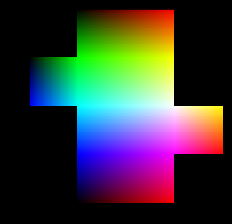
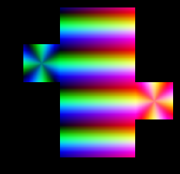
Figure 1: Two representations of the surface points of a $4$-fold symmetric box as color coded $3D$-vectors (unwrapped): left plain object points, right the proposed closed symmetry loop or star representation. The right is continuous and respects symmetry, whereas the left does not.

I-B This Work’s Contribution and Structure

• a mathematical analysis which properties a CNN output representation must have to represent the pose of a symmetric object in a continuous way (Sec. II);

• an investigation with a 1-DOF toy problem that demonstrates the effect the continuity problem has for common representations and motivates a solution (Sec. III);

• an algorithm for 6-DOF pose estimation based on this idea, extending [1] to symmetric objects (Sec. IV) and

• an evaluation on the T-LESS benchmark dataset showing competitive results (RGB 46.8, RGBD 58 AR) (Sec. V).

Finally, Section VI relates the observations to prior work and Section VII concludes. The source code of this work is available.

II Mathematical Motivation

This section motivates the approach to define the output of the CNN as a specialized representation that reflects the symmetry of the underlying object and derives what structure this representation needs to have. Consider an object with $n$-fold, i.e. $\theta=\frac{2\pi}{n}$, rotational symmetry around the $Z$-axis. Let $\operatorname{Rot}_{z}(\alpha)$ be rotation around $Z$ and $f$ be a “render” function that maps for a fixed object and scene, a pose to an image of the object in that pose. Since the object is symmetric

$$f(T)=f\left(T\operatorname{Rot}_{Z}\left(i\theta\right)\right)\quad\forall T\in SE(3),i\in\mathbb{Z}$$ (1)

Note that $f$ is continuous, as small changes in pose lead to small changes in the image. Now let $g$ be the function learned by the CNN, mapping from an image to some representation of the pose by real numbers $\in\mathbb{R}^{m}$. Examples from the literature are a matrix, a quaternion, a heatmap of bounding-box corners [3], object-coordinates per pixel [7] or any other suitable representation. Now being a CNN, $g$ is continuous and $f$ is continuous as well, so for a given $T\in SE(3)$,

$$h:\left[0\ldots\theta\right]\rightarrow\mathbb{R}^{m},\quad\alpha\mapsto g(f(T\operatorname{Rot}_{Z}(\alpha)))$$ (2)

is a continuous function. It is also injective except for $0$ and $\theta$ because all poses in between are not equivalent even with symmetry. So $h$, i.e. the pose representation for continuously rotating by one step of symmetry, is a simple closed curve. This is not possible for any above mentioned representation, where rotating by $2\pi$ is a simple closed curve but by $\theta$ is not. Note that this is true, regardless whether the pose representation is “interpreted modulo $\theta$” later, because CNNs cannot represent functions that are continuous in some modulo topology but not in the usual $\mathbb{R}^{m}$ topology.

Of course a CNN can also learn to approximate an uncontinuous function. Probably it will be steep (but still continuous) at a gap of the training data, since that does not affect the training loss. So we can conclude that by choosing a pose representation that does not reflect the objects $n$-fold symmetry, we force the network to approximate an uncontinuous function and give rise to generalization problems.

III 1-DOF Toy Problem Investigation

We will now analyze a toy problem that is simple enough, so we can plot the CNN’s behavior on the whole input data, but still exhibit the above mentioned phenomenon: A rotating disc with textured perimeter is viewed from the side by a line-camera (Fig. 2a). The disc’s texture has an $n=6$-fold symmetry, i.e. the angle of symmetry is $\theta=2\pi/n=\pi/3\approx 1.05$ (cyan lines in Fig. 2). From the obtained 1D-image (Fig. 2b), a CNN shall estimate the rotation angle $\alpha$ of the disc as $\hat{\alpha}$. We are interested in how well the CNN can learn this task for different representations of the angle as output and different corresponding losses.

As the focus is on the output representation and the problem is rather simple, we use a canonical encoder-head architecture, details can be seen in the implementation. Our training dataset has images at $\pi/180$ spaced angles, the test set at $\pi/900$ spaced. We trained every CNN 11 times and report on the network with the median loss.

III-A Outputs representing an angle

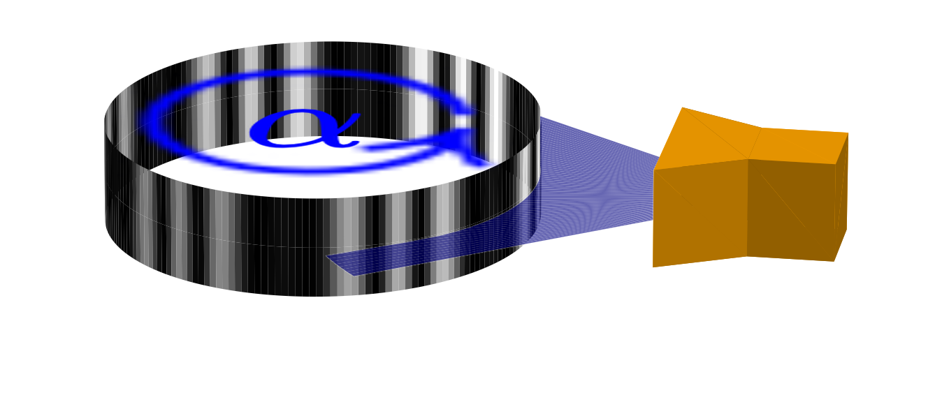
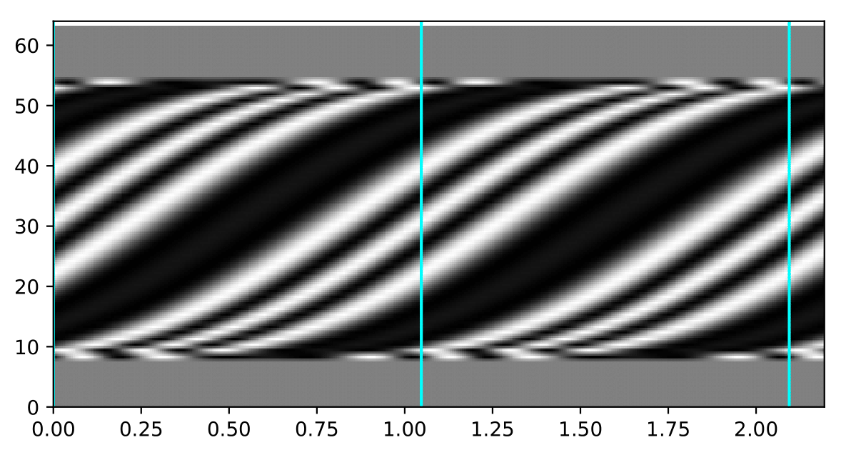
a) disc and camera	b) 1-D images over $\alpha$
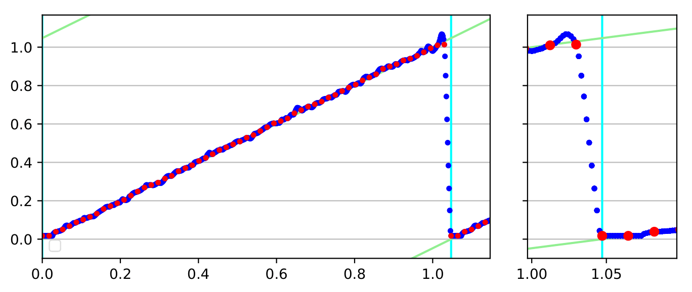
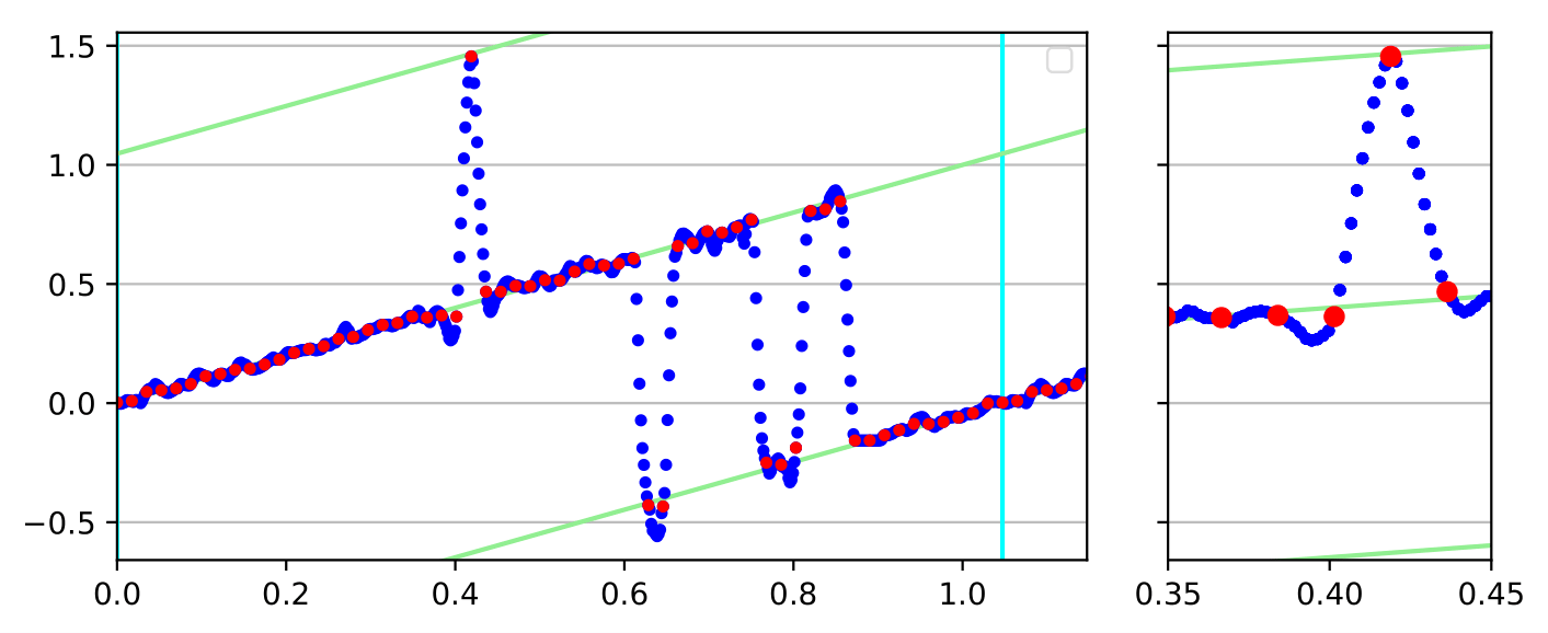
c) norm. angle / ae	d) angle / mos-ae
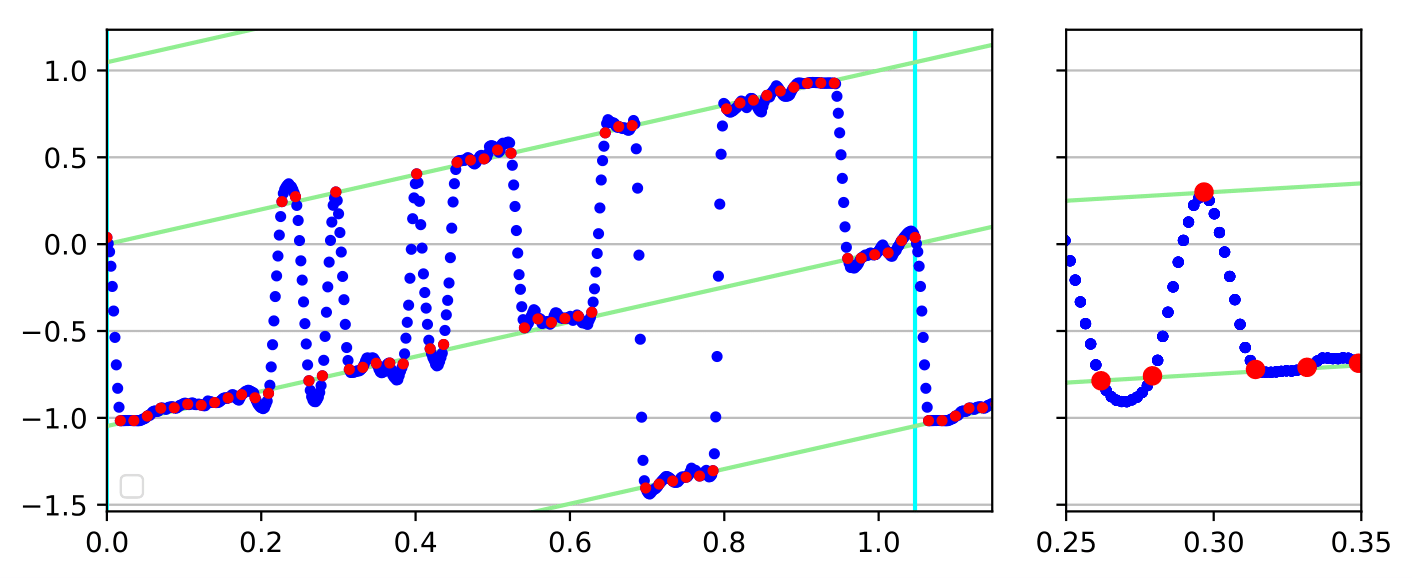
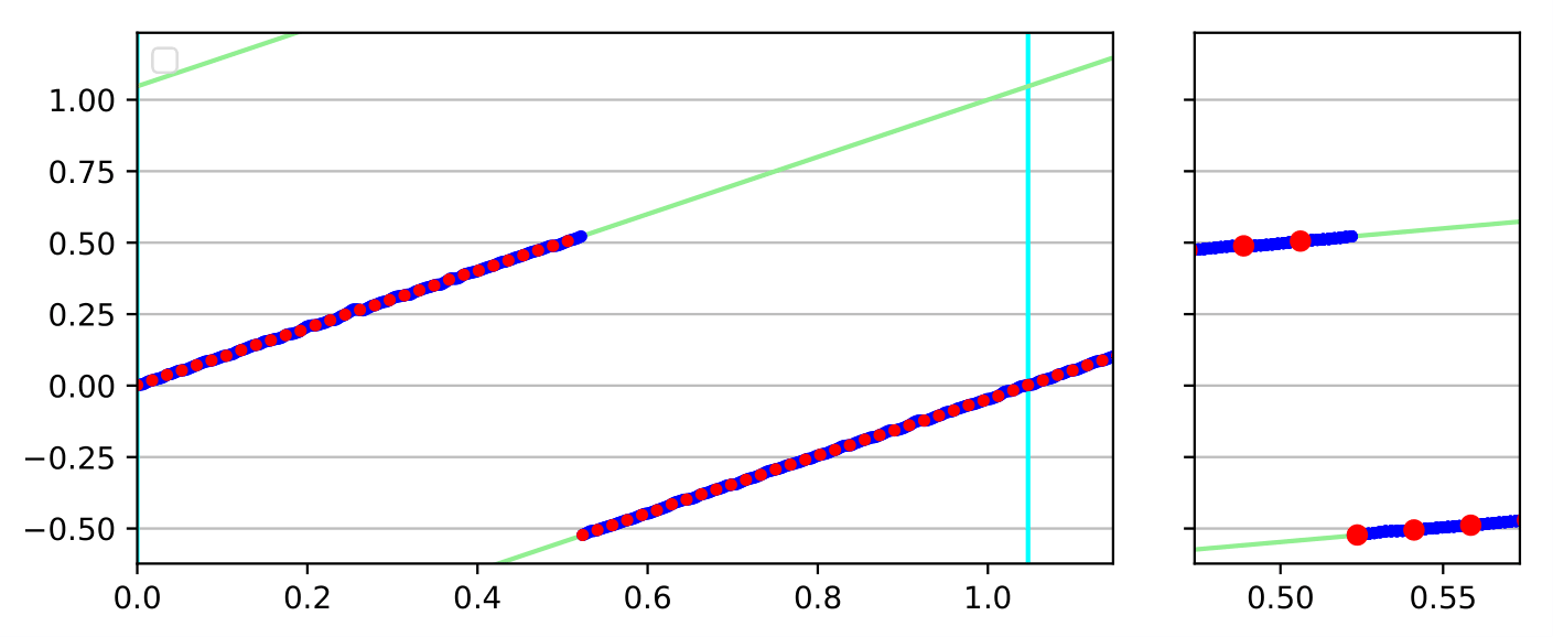
e) vector / mos-ae	f) csl-vector / ae
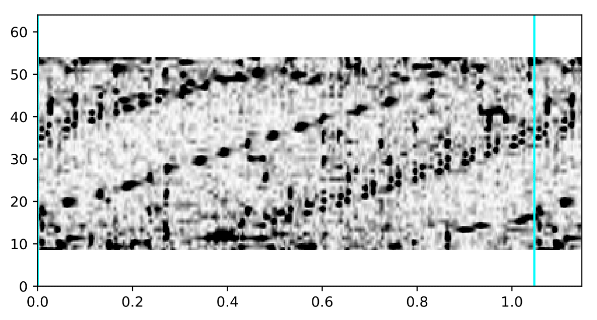
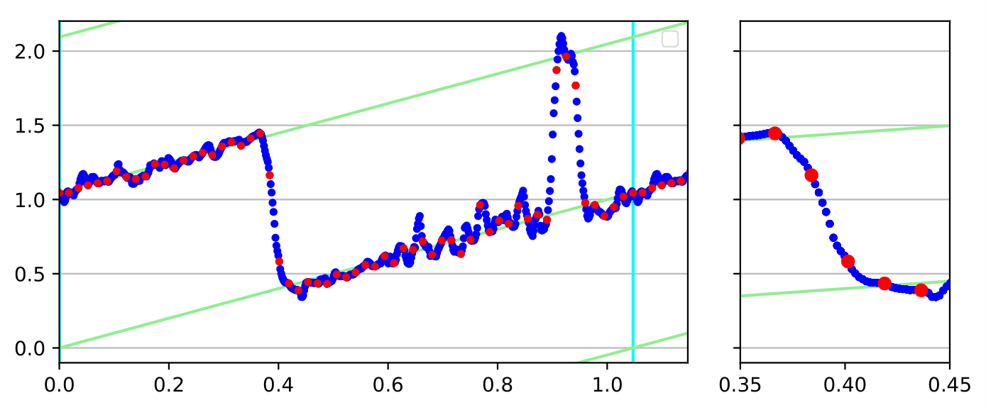
g) $p^{O}$-img / px-mos-ae	h) center pixel of g)
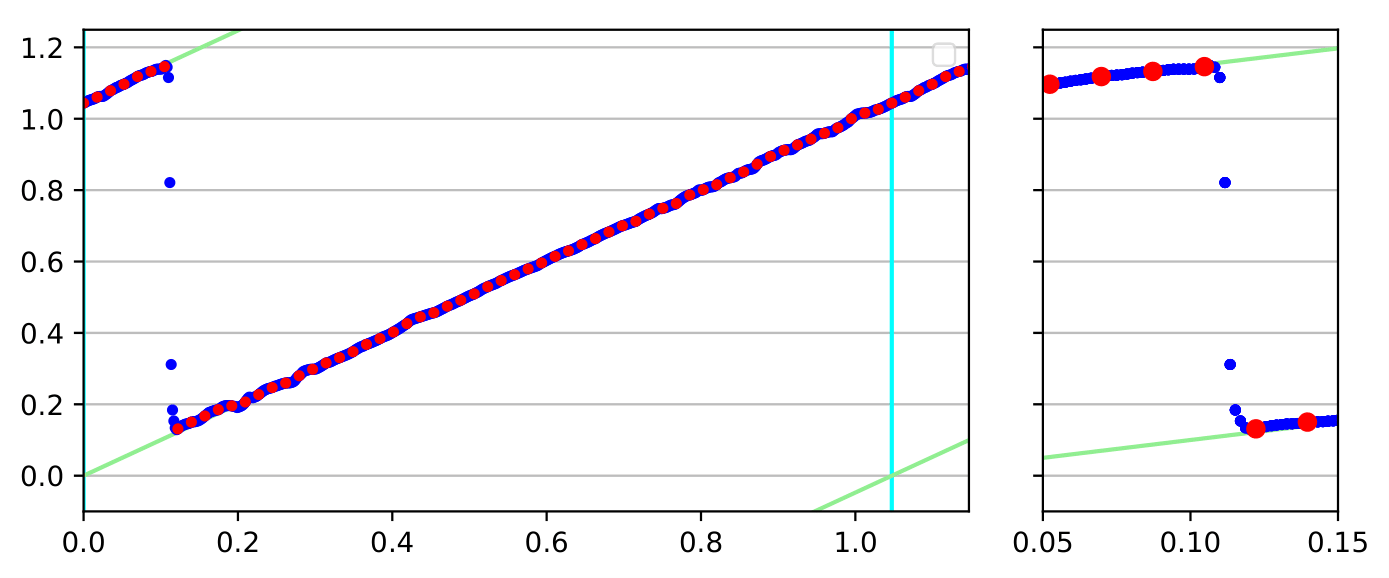
i) $p^{O}$-img / img-mos-ae	j) center pixel of i)
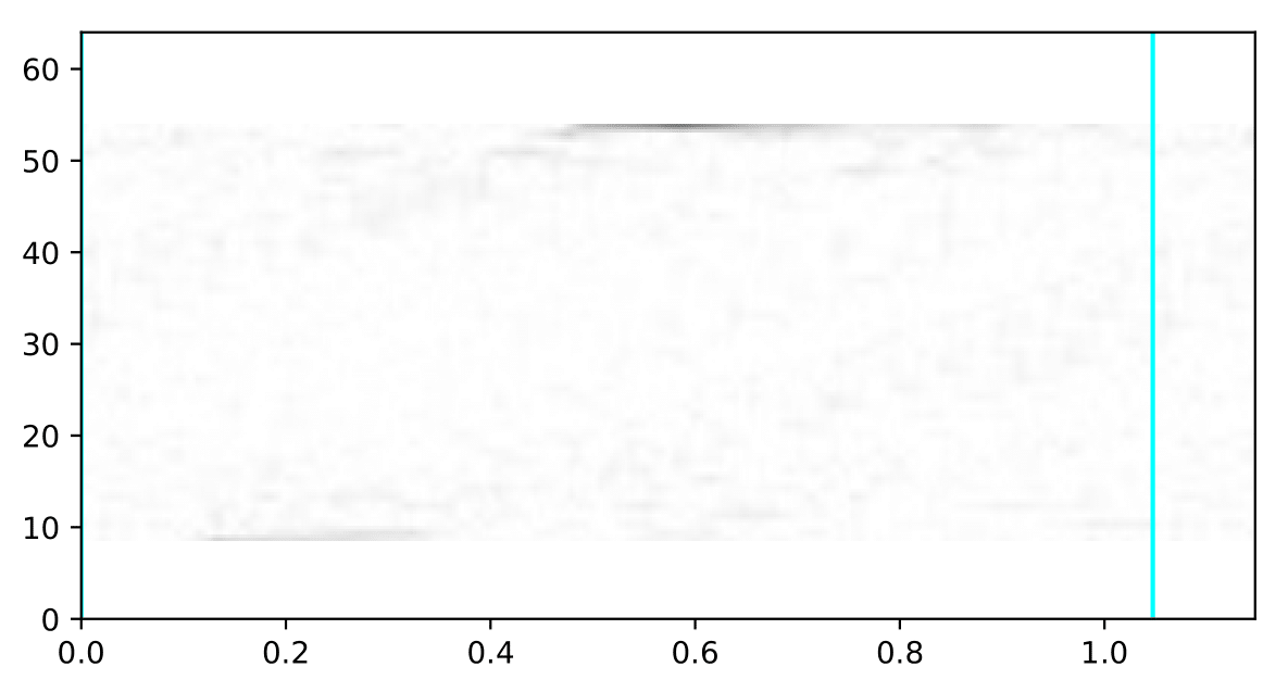
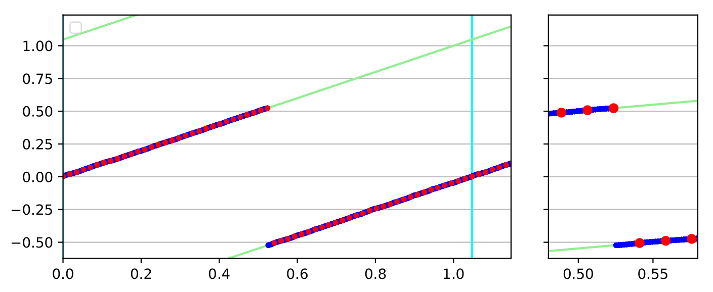
k) $p^{O}$-img / ae	l) center pixel of k)

Figure 2: Comparing different output representations for the angle of a rotating disc with 6-fold symmetric texture. In all plots the ground truth angle is shown on the x-axis and the cyan vertical lines indicate periodicity, the ground truth and its symmetric equivalents are shown in green, the CNN prediction converted to an angle in blue and the prediction on training data is highlighted in red. g/i/k show the error of the represented object points (black=large). See Sec. III for details.

We initially consider the task to estimate $\alpha$ the disc orientation in some representation.

The first output representation is normalized angle $\in[0\ldots\theta[$ with an absolute error loss:

$$y^{\text{norm. angle}}=\alpha-\theta\lfloor{\tfrac{\alpha}{\theta}}\rfloor,\quad\mathcal{L}^{\text{ae}}(y,\hat{y})=|y-\hat{y}|,$$ (3)

where $y$, $\hat{y}$ and $\mathcal{L}$ are groundtruth output, predicted output and loss of a sample, which has groundtruth disc angle $\alpha$. The representation forms no closed loop, so the CNN has to approximate the discontinuity at $\theta$ by a steep transition. It does so (Fig. 2c) by placing the transition between two training samples, so it is invisible in the loss, but creates a small region of large (up to $\theta/2$) generalization error.

The second idea is to use the angle, but interpret it “modulo $\theta$” by viewing it as the set of all symmetric equivalents. Canonically, the distance to a set is defined as minimum distance over its elements. This leads to the minimum-over-symmetries absolute error (mos-ae) loss:

$$y^{\text{angle}}=\alpha,\quad\mathcal{L}^{\text{mos-ae}}(y,\hat{y})=\min_{k\in\mathbb{Z}}|y-\hat{y}+k\theta|$$ (4)

This appears like an elegant solution. However, it does not form a closed loop as the output at $0$ and $\theta$ is not equal but only equivalent. So it also requires the CNN to learn a discontinuity creating a transition. The experimental result is even worse, making many apparently unnecessary transitions on the way (Fig. 2d). Presumably, these appear when in early learning stages different symmetric equivalents of the groundtruth are closest and the loss pulls the CNN towards these. Later, the solution can not move from one equivalent to another, as they are separated by a barrier of large loss. This observation sheds doubt on the effectiveness of the minimum-over-symmetries approach.

The third idea replaces the angle by a unit vector to eliminate the $2\pi$-wraparound:

$$y^{\text{vector}} =\operatorname{cart}\left(\begin{smallmatrix}\alpha\\ 1\end{smallmatrix}\right),\;\mathcal{L}^{\text{mos-ae}}(y,\hat{y})=\min_{k\in\mathbb{Z}}|\operatorname{Rot}(k\theta)y-\hat{y}|,$$ (5)

$$\text{with }\operatorname{cart}\left(\begin{smallmatrix}\phi\\ \rho\end{smallmatrix}\right)=\left(\begin{smallmatrix}\cos\phi\rho\\ \sin\phi\rho\end{smallmatrix}\right)\!,\;\operatorname{Rot}{\phi}=\left(\begin{smallmatrix}\cos\phi&-\sin\phi\\ \sin\phi&\cos\phi\end{smallmatrix}\right)$$ (6)

It is still not a closed loop and $2\pi$ is actually not the problem, because $\theta$ is. Correspondingly, this approach performs not better than the previous (Fig. 2e).

The proposed closed symmetry loop (csl) vector representation starts from the observation that the vector representation forms a closed loop over $[0\ldots 2\pi]$. Hence, we multiply the angle by $n$ before turning it into a vector. So $\theta$ becomes $2\pi$ and the csl vector forms a closed loop over $[0\ldots\theta]$. The representation respects symmetry, mapping symmetric equivalents to the same value:

$$y^{\text{csl vector}}=\operatorname{cart}\left(\begin{smallmatrix}n\alpha\\ 1\end{smallmatrix}\right),\quad\mathcal{L}^{\text{mos-ae}}(y,\hat{y})=|y-\hat{y}|$$ (7)

With this representation the CNN learns a function without transitions (Fig. 2f). Note that the discontinuity in the graph comes from converting the vector back to an angle for plotting and does not appear in the output itself.

III-B Outputs Representing an Object Point Image

We now turn towards a more complex but related problem, which we need in [1] and Sec. IV later. Here, the output is an image, where each pixel indicates the point of the object seen in that pixel in object coordinates ($p^{O}$-image). So the CNN answers the question “What do you see here?” and the final object pose is obtained by a perspective n-point (PnP) problem from that. Different reprensentations and corresponding losses for $p^{O}$ are possible, which we will investigate here. We therefor extend the CNN to a canonical encoder/decoder with shortcuts architecture.

The first idea uses a $p^{O}$-image representation where each pixel of the output is the 2D vector of the seen point in object coordinates. Symmetry is again handled by a min-over-symmetries loss. It takes the average over all pixels of the minima (pmos-mae), thereby allowing each pixel to choose its own symmetric equivalent.

$$y^{\text{$p^{O}$-img}}_{i}\!\!=\!\!p^{O}_{i},\;\mathcal{L}^{\text{pmos}}_{\text{-mae}}(y,\hat{y})=\tfrac{1}{m}\sum_{i}\min_{k\in\mathbb{Z}}|\operatorname{Rot}(k\theta)y_{i}-\hat{y}_{i}|,$$ (8)

where $p^{O}_{i}$ is the true point of the disc visible at pixel $i$ and $m$ is the number of pixels. Fig. 2g/h show the result with a large error and many unnecessary transitions.

output repres.	loss	pixel error	angle error
normalized angle	ae (3)		0.0099
angle	mos-ae (4)		0.0378
vector	mos-ae (5)		0.0660
csl vector	ae (7)		0.0020
$p^{O}$ image	pmos-mae (8)	0.0703	0.0092
$p^{O}$ image	imos-mae (9)	0.0074	0.0045
csl image	mae (10)	0.0029	0.0005

TABLE I: Error of CNNs with different output representations. Abbr.: (p/i)mos - (pixel/image) min over symmetries, csl - closed symmetry loop (proposed), $p^{O}$: object point

The second idea also uses a $p^{O}$-image but takes the min of the averages, i.e. per image (imos-mae). This forces consistency, i.e. all pixels choose the same equivalent.

$$y^{\text{$p^{O}$-img}}_{i}=p^{O}_{i},\;\mathcal{L}^{\text{imos}}_{\text{-mae}}(y,\hat{y})=\tfrac{1}{m}\min_{k\in\mathbb{Z}}\sum_{i}|\operatorname{Rot}(k\theta)y_{i}-\hat{y}_{i}|\!\!\!$$ (9)

Fig. 2i/j show that imos-mae is much better than pmos-mae. This is surprising, because the optimal $k$ from (9) is also a valid choice for all $i$ in (8). Thus $\mathcal{L}^{\text{pmos-mae}}(y,\hat{y})\leq\mathcal{L}^{\text{imos-mae}}(y,\hat{y})$. However, as with mos-ae, pmos-ae attracts the CNN early to different symmetric equivalents, creating unnecessary transitions. By forcing consistency in one image, it also supports consistency over angles, because images at similar angles mainly differ by a translation for which a CNN is invariant. Still, it forms no closed loop, the CNN has to learn one discontinuity and there is one transistion because of that. Fig. 2i shows that all pixels perform this transition at the same angle, to maintain consistency in the images.

Finally, the proposed csl image representation for the $p^{O}$ also called $p^{O*}$ forms a closed loop when continuously rotating by $\theta$ and can use a simple mae loss. It takes the $p^{O}$ vector in every pixel and multiplies its angle by $n$. As with the csl vector representation, a rotation by $\theta$ is mapped to a rotation by $2\pi$, which is a closed loop.

$$y^{\text{csl img}}_{i}\! =\!p^{O*}_{i}\!=\!\operatorname{cart}\bigl{(}\left(\begin{smallmatrix}n&\\ &1\end{smallmatrix}\right)\operatorname{pol}\left(\begin{smallmatrix}p^{O}_{i}\end{smallmatrix}\right)\bigr{)},\;\operatorname{pol}\left(\begin{smallmatrix}x\\ y\end{smallmatrix}\right)=\left(\begin{smallmatrix}\operatorname{atan2}(y,x)\\ \sqrt{x^{2}+y^{2}}\end{smallmatrix}\right),$$

$$\mathcal{L}^{\text{ae}}(y,\hat{y})=\tfrac{1}{m}\sum_{i}|y_{i}-\hat{y}_{i}|$$ (10)

Fig. 2k/l show that there is no transition, the visible discontinuity comes again from plotting the result as an angle.

III-C Discussion

Table I compares all representations quantitatively. If the representation is an image, both the average per pixel error and the error of the final angle is given. This is obtained by simply comparing to a precomputed list of object point images with interpolation. In the 3D scenario, later, this is a more complex PnP problem.

We conclude with three insights: First, minimum-over-symmetries losses, while mathematically elegant, tend to not work well with gradient-based optimization of a CNN. Second, letting the CNN output an object point image from which the pose is geometrically computed is more precise than letting the CNN directly output the pose. Third, by multiplying the angle of a vector with the order of the symmetry, we can define the star representation that forms a closed loop and makes the function to be learned continuous and that achieved the lowest error in this study.

IV Approach (6-DOF)

Following the above considerations, we modified our previous representation [1] in a symmetry-specific way, such that rotating by one step of symmetry, i.e. $\theta=\frac{2\pi}{n}$, is a simple closed curve in the representation.

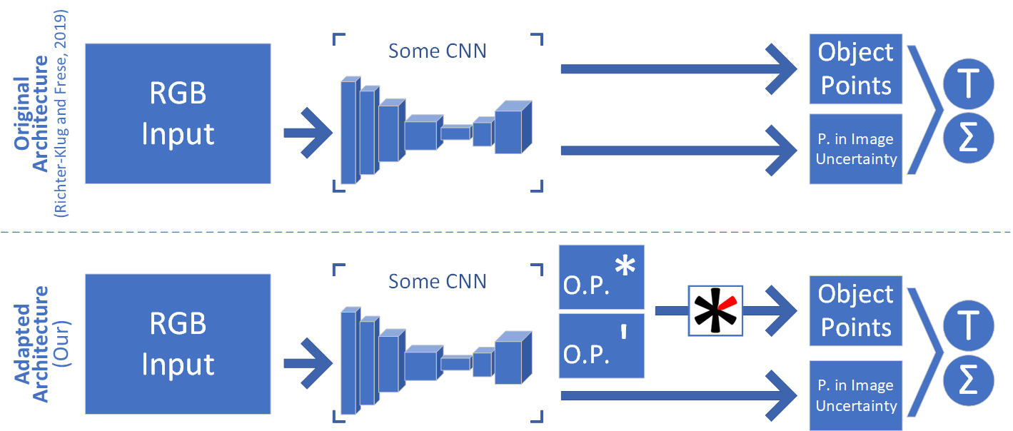
Figure 3: Network architecture extension overview adapted from [1]. Originally (top), an RGB image is fed into a CNN, which outputs the seen object point (per pixel) as well as an estimate of their in-image uncertainties. This information is then combined by PnP with all the pixels that belong to the same object to estimate its pose ($T$) and 6d uncertainty ($\Sigma$). In this paper (bottom), we adapt this architecture with a symmetry-aware but ambiguous object point representation (star), which is aided by the dash representation, both predicted by a CNN. They are then combined to regain the object points, followed by the unchanged PnP stage.

In the originally proposed architecture, the CNN predicted object points densly. These were regressed by PnP for getting a pose estimate. In addition, the CNN predicted in-image uncertainty for each found object point. Therefore, the PnP could also provide a 6d uncertainty estimate (Fig. 3-top).

To make this architecture symmetry-aware, we change the CNN’s object point output to a symmetry-aware one, the so-called star representation (Sect.IV-A), and regain valid object points before the PnP stage (but outside of the CNN) by reversing the representation’s modification (Sect.IV-C). A second CNN output, the so-called dash representation (Sect.IV-B) helps by untangling the object point ambiguities caused by the symmetry (Fig. 3-bottom, Fig. 4, Fig. 5).

IV-A The star representation of object points

The representation is a modification of the object points such that rotating by one step of symmetry, i.e. $\frac{2\pi}{n}$, is a simple closed curve in the representation (csl-image). In it, all object points, that appear the same (based on the defined symmetry), are mapped on the same value and no possible rotation will result in an uncontinuous change. Therefore, the representation becomes symmetry aware, but also ambiguous.

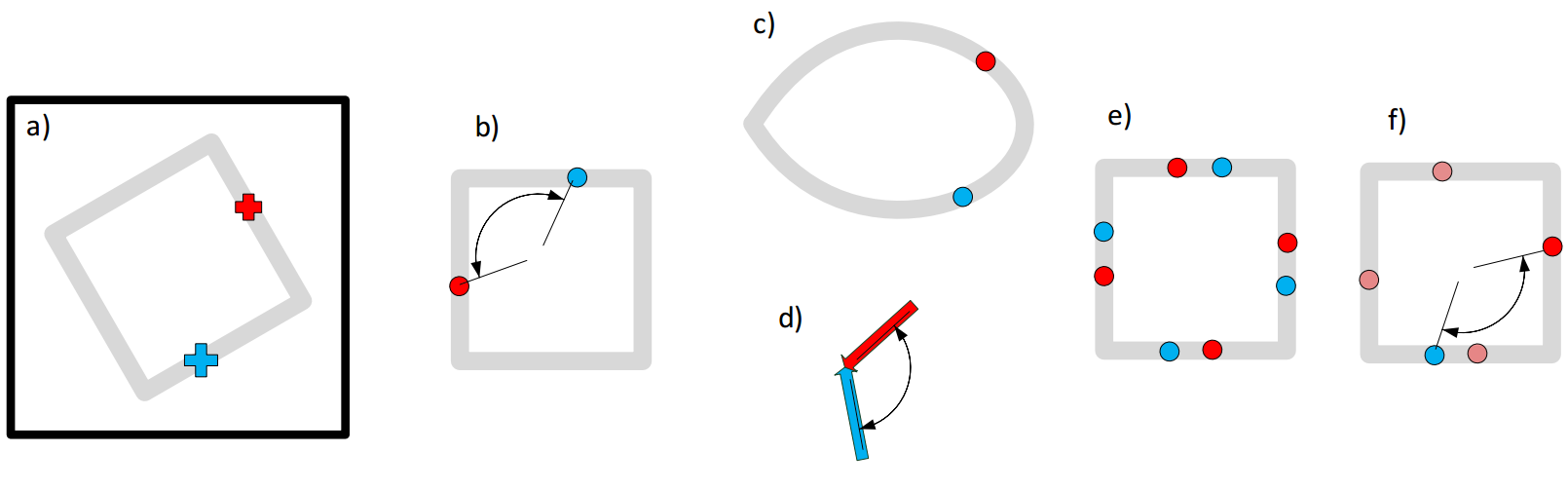
Figure 4: Steps of the forth and back transformation with two points marked as examples. All quantities are actually 3D vectors, here we show X and Y for clarity, Z is the axis of symmetry. a) the image perceived by a camera looking on a box from above. b) object points $p^{O}$ as used in [1], c) $p^{O*}$ information predicted by the CNN, d) $p^{O^{\prime}}$ information also predicted by the CNN, e) $P^{O}$ equivalence classes obtained from $p^{O*}$, f) consistent disambiguation of the $P^{O}$ using $p^{O^{\prime}}$ to regain $p^{o}$. (blue:arbitrarily chosen reference $p_{r}$, red: best fitting point from equivalence class $P^{O}$)

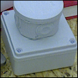
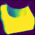
a) RGB input	b) segmentation	c) true object points
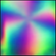
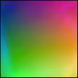
d) star output	e) dash output	f) new object points

Figure 5: Example input image a) with object segmentation b) and the unknown true object points c). The proposed reverse operation uses our outputs d) and e) to genereate the object points f). These are then used to estimate the object’s pose. Note that f) is not equal to c) but it could have been. In this specific case, it is instead offsetted by two steps of symmetry.

To gain the star representation of the object points, these are first transformed in cylindrical coordinate space, where the cylindric axis is aligned with the symmetry axis. Here the angle value is multiplied by $n$ (the fold of symmetry). Afterwards the points are transformed back to Cartesian vector space (Fig. 4c).

$$p^{O*}_{ij} =\operatorname{cart}\Bigl{(}\left(\begin{smallmatrix}n&&\\ &1&\\ &&1\end{smallmatrix}\right)\operatorname{cyl}(p^{O}_{ij})\Bigr{)},$$ (11)

$$\text{with }\operatorname{cart}\left(\begin{smallmatrix}\rho\\ \psi\\ z\end{smallmatrix}\right) =\left(\begin{smallmatrix}\rho\cos\psi\\ \rho\sin\psi\\ z\end{smallmatrix}\right),\quad\operatorname{cyl}\left(\begin{smallmatrix}x\\ y\\ z\end{smallmatrix}\right)=\left(\begin{smallmatrix}\operatorname{atan2}(y,x)\\ \sqrt{x^{2}+y^{2}}\\ z\end{smallmatrix}\right)$$ (12)

For clarity, this assumes, w.l.o.g. Z as symmetry axis.

Note that the CNN is trained to output $p^{O*}$ so the computation in (11) is not executed when using the algorithm but when preparing the ground truth output for training.

Let’s have a closer look at the folds of symmetry extremes: On the lower end, one finds non-symmetrical objects ($n=1$); In this case the star representation is identical to the origin object points which is the expected outcome. On the other end, we find objects with infinity-fold symmetries, e.g. bottles. Here an infinitely small step of rotation closes one step of symmetry. Since the multiplication with infinity is unhandy, in this case, we multiply the angle values with zero. Therefore, all points have the same angle around the rotation axis as they all are equivalent under symmetry.

IV-B The dash representation of object points

The ambiguity of the star representation causes ignorance whether two points, whose values are close, also lie close on the object or e.g. on opposing ends. But, this information is needed to regain an object point that is consistent with all points in view (cf. IV-C). We argue that this information can be seen inside an image despite or rather independently of any possible symmetries and therefore is extractable.

As such information we use the pixelwise object points rotated into the camera. This is minus the vector from the object point to the object’s origin relative to the camera. We argue that this vector is observable in the image and hence can be predicted by a CNN. Note, this information is innately symmetrical invariant and (since we only rotated the object points) all angles between any object points are preserved, but no information regarding the object’s rotation itself (Fig. 4d).

The selected information can not be learned as is, since orientation is not a translation invariant function of the image (cf. [1, Fig. 2]). Thus, depending on the pixel position in the image, we rotate the vector, such that the CNN can treat it as if in the image center. Formally,

$$p^{O^{\prime}}_{ij} =R_{ray}^{-1}(i,j)\;R^{C}_{O}\;p^{O}_{ij},$$ (13)

$$R_{ray}(i,j) ={\;}^{\operatorname{angle}}_{\operatorname{axis}}\biggl{(}\sphericalangle\Bigl{(}\left(\begin{smallmatrix}0\\ 0\\ 1\end{smallmatrix}\right),\operatorname{ray}(i,j)\Bigr{)},\left(\begin{smallmatrix}0\\ 0\\ 1\end{smallmatrix}\right)\times\operatorname{ray}(i,j)\biggr{)}$$ (14)

$R_{ray}(i,j)$ is a matrix rotating the Z-axis onto the viewing ray of pixel $(i,j)$. The viewing rays are defined by the camera calibration.

Note that before this representation’s usage (i.e. IV-C) the rotational offset must be reversed.

IV-C The reverse operation

The purpose of the reverse operation is to gain an image of object points that together define a pose in the PnP stage that is right up to the object’s symmetry. Each point in the star representation defines an equivalence class of object points (Fig. 4e) that can be extracted by reversing (11) as

$$P^{O}_{ij}\!=\!\left\{\!\operatorname{cart}\biggl{(}\!\!\left(\begin{smallmatrix}\tfrac{1}{n}&&\\ &1&\\ &&&1\end{smallmatrix}\right)\!\!\operatorname{cyl}\Bigl{(}p^{O*}_{ij}\Bigr{)}\!+\!\left(\begin{smallmatrix}k\theta\\ 0\\ 0\end{smallmatrix}\right)\biggr{)}\bigg{|}k\in[0\ldots{}n[\right\}\!.\!\!\!$$ (15)

Although each point of the equivalence class would be per se valid, only a consistent choice over all recognized points of an object will lead to a correct pose prediction. Two points are chosen consistently if their offset equals their true offset, e.g. if two points oppose each other opposing object points must be chosen, too. To determine the offset between two object points, the dash representation was introduced. In it, the angle between two vectors is the same as between their corresponding object points, if selected consistently (cf. IV-B). This is utilized in the following procedure for selecting consistent points from the equivalence sets (15).

Three noncollinear object points with corresponding dash representations are selected as reference $R$. Then a consistent choice for all other equivalence classes can be made by selecting the equivalent with the smallest sum of angle errors to all reference points (Fig. 4f):

$$p^{O}_{ij} =\arg\min_{p\in P^{O}_{ij}}\;\;\sum_{(p_{r},p^{\prime}_{r})\in R}\;\big{|}\sphericalangle(p,p_{r})-\sphericalangle(p^{O^{\prime}}_{ij},p^{\prime}_{r})\big{|}$$ (16)

For continuous rotational objects such as bottles, a point in the star representation maps to an infinite equivalence class $P^{O}_{ij}$. Methodically, we thus want an infinite $\arg\min$ in (16). For practical reasons, this is replaced by $\tilde{P}^{O}_{ij}$, which contains for every reference point the two possible object points with the desired angle $\sphericalangle(p^{O^{\prime}}_{ij},p^{\prime}_{r})$. These points are obtained by first rotating an arbitrary point $\bar{p}^{O}$ from the equivalence class above each reference point ($\bar{\bar{p}}^{O}$). These points are then rotated by the angles $\pm\beta$ obtained by the spherical Pythagorean theorem to get the desired two points.

$$\tilde{P}^{O}_{ij} =\Bigl{\{}\operatorname{Rot}_{Z}(\pm\beta)\bar{\bar{p}}^{O}\Big{|}(p_{r},p^{\prime}_{r})\in R\Bigr{\}},\text{ with a }\bar{p}^{O}\in P^{O}_{ij},$$ (17)

$$\beta =\arccos\left(\frac{\cos\sphericalangle(p^{O^{\prime}}_{ij},p^{\prime}_{r})}{\cos\sphericalangle(\bar{\bar{p}}^{O},p_{r})}\right)\!\!,\;\bar{\bar{p}}^{O}=\operatorname{cart}\left(\begin{smallmatrix}\operatorname{cyl}(p_{r})_{\phi}\\ \operatorname{cyl}(\bar{p}^{O})_{\rho}\\ \operatorname{cyl}(\bar{p}^{O})_{Z}\end{smallmatrix}\right)\!\!.$$ (18)

For clarity, this assumes $Z$ as symmmetry axis.

As reference $R$, any three noncollinear object points with corresponding dash representation can be selected, e.g. one of the possible object point combinations with the smallest angle error sum for three arbitrary selected output pixel. The rotational axis inside the dash representation can be regressed. For continuous rotational objects, this can be used to form a reference based on the coordinate system, since the other two axis may be selected arbitrarily (if they form a coordinate system).

V Experimental 6-DOF Evaluation

We evaluate our approach on the T-LESS Dataset [8] which spotlights 30 industry-relevant objects without discriminative color and texture. Regarding the symmetry the objects can be categorized in eleven $\infty$-fold, $15$ $2$-fold, three $1$-fold and one $4$-fold symmetry around one axis. We accessed the dataset via the ”BOP: Benchmark for 6D Object Pose Estimation” which provides standardized simulated training data, evaluation methods and the results from other state-of-the-art algorithms for direct comparison (cf. [2]). Since we only improve the pose estimation, we use the mask R-CNN detector results from [9] for evaluation.

V-A Network Structure and Learning Procedure

As network structure we use a DenseNet[10]-like encoder-decoder structure with horizontal connections. All (non-output) convolutions are activated by SELU [11]. As optimizer, Adam [12] is used with the amsgrad expansion [13] and a learning rate of $0.0001$. Our network is trained in two phases: We pretrain the object point relevant outputs for two epochs. Afterwards, we include also the uncertainty outputs. The therefore complete network is then trained for additional ten epochs. More details can be seen in our implementation.

For training, we generated ten samples for each training datum provided by [2]. For each sample a scale and translation offset is drawn from Gaussian distributions. Additionally, all input images are augmented by contrast, Gaussian and brightness noise and always processed as grayscale images since the objects are colorless.

V-B Results

Method (RGB)	refinement	AR	ARMSPD
CosyPose [9]	RGB	72.8	82.1
Ours	-	55.2	76.5
CDPN [14]	-	49.0	67.4
CDPNv2 [14]	-	47.8	62.0
EPOS [15]	-	47.6	63.5
leaping from 2D to 6D[16]	-	40.3	71.2
Pix2Pose [3]	-	34.4	47.6

TABLE II: Average recall (AR) on the T-Less dataset (RGB only, cf. [2])

Method (RGB-D)	refinement	AR	time (s)
CosyPose [9]	RGB+ICP	70.1	13.74
König [17]	ICP	65.5	0.63
Ours w. depth fusion	-	65.1	0.45
Vidal [18]	ICP	53.8	3.22
Pix2Pose [3]	ICP	51.2	4.84
Drost-Edges [19]	ICP	50.0	87.57
Sundermeyer [20]	ICP	48.7	0.86
CDPNv2 [14]	ICP	46.4	1.46

TABLE III: Average recall (AR) on the T-Less dataset (RGB-D, cf. [2])

Table III shows our average recall (AR, as defined in [2]) on the T-LESS dataset in comparison to other state-of-the-art methods for RGB-only processing. Our approach reaches state-of-the-art results and is only exceeded by a approache with refinement steps i.e. CosyPose [9]. Since the T-LESS dataset comprises mainly symmetric objects (28/30), it stands to reason that the proposed approach aids CNNs to converge better.

Since we build upon [1], which introduced a simple method for utilizing the depth image’s information by fusing it directly into the PnP stage, we are able to integrate depth data as well. Our results with depth fusion in comparison to state-of-the-art results on RGB-D can be seen in Table III. We are the only algorithm not refining with an ICP-variant. Therefore, our predictions are calculated noticeably faster (cf. III). Nevertheless, our results on RGB-D data are competitive.

VI Related Work

The problem of symmetry in CNN-based 6D-Pose detection is also discussed in [21]. This work, as well as [22] propose a simple normalization of the pose’s rotation. Naturally, this introduces an uncontinuity after one rotation of symmetry, wherefore they furthermore propose to learn a second, offsetted, normalization per symmetry. This normalization is of course also uncontinuous but at a different angle. Finally, a special segmentation is learned in addition to the normalized rotations, which only use is to indicate in which normalization’s sweet spot the perceived rotation lies and therefore which normalization output should be used to calculate the pose. This approach is also used in e.g. [9] or [23].

Instead of learning 3D object coordinates in one way or another, Hodan et al. [15] split at first the objects into surface fragments for which then coordinates and probabilities are learned. The probability of one fragment indicates how likely this fragment is seen, given the originating object is observed. Afterwards, the position for each fragment can be calculated and the pose can be extracted by solving a PnP variant over these fragment. Note that multiple fragments can live next to each other on the same spot, which is only disentangled inside the PnP-RANSAC for many-to-many 2D-3D correspondences. This approach can handle symmetry by learning multiple fragments with the same appearance, which should get the same probability assigned by the CNN. In this approach, the learned coordinates (of the segments) are not biased by uncontinuity as long as the segments are selected sufficiently small since each segment for itself is not symmetric. While this representation inflates the output space, it has the additional advantage of working without knowledge of the object’s symmetry. Interestingly, this approach (which is strongly different but also not biased by uncontinuity) reaches highly comparable results to this work (cf. table III).

The importance of continuity of the rotational representation for a CNN in general was also investigated and affirmed by [24], however they did not consider symmetries.

Peretroukhin et al. [25] represent rotations implicitly as a quaternion defined by $q^{*}=\arg\min_{|q|=1}q^{T}Aq$ for a $4\times 4$ matrix $A$ which is the output of the network. It defines a Bingham distribution and according to the authors measures uncertainty, even if instead of likelihood only a loss on $q*$ was trained. This is related to the $T^{*}=arg\min_{T\in{}SO(3)}\bar{T}^{T}(M^{T}M)\bar{T}$ representation we use [1] for a rotation matrix $T$ flattened as $\bar{T}$. Unlike [25], it represents pose distributions resulting from perspective observations.

VII Conclusions

In this work we analysed the effect of symmetric objects on CNN-based pose estimation. We show that without special care, a CNN has to approximate an uncontinuous function which is not optimal. In contrast, we propose a method to warp the CNN’s output space in such a way that the uncontinuity is moved to postprocessing outside the CNN. Our updated methode reaches state-of-the-art on the T-LESS dataset for unrefining RGB-based methods with an AR of $55.2$.

References

- [1] J. Richter-Klug and U. Frese, “Towards meaningful uncertainty information for cnn based 6d pose estimates,” in International Conference on Computer Vision Systems. Springer, 2019, pp. 408–422.
- [2] T. Hodan, M. Sundermeyer, B. Drost, Y. Labbe, E. Brachmann, F. Michel, C. Rother, and J. Matas, “BOP challenge 2020 on 6d object localization,” arXiv preprint arXiv:2009.07378, 2020.
- [3] K. Park, T. Patten, and M. Vincze, “Pix2pose: Pixel-wise coordinate regression of objects for 6d pose estimation,” in Proceedings of the IEEE International Conference on Computer Vision, 2019, pp. 7668–7677.
- [4] H. Wang, S. Sridhar, J. Huang, J. Valentin, S. Song, and L. J. Guibas, “Normalized object coordinate space for category-level 6d object pose and size estimation,” in Proceedings of the IEEE Conference on Computer Vision and Pattern Recognition, 2019, pp. 2642–2651.
- [5] C. Wang, D. Xu, Y. Zhu, R. Martín-Martín, C. Lu, L. Fei-Fei, and S. Savarese, “Densefusion: 6d object pose estimation by iterative dense fusion,” in Proceedings of the IEEE Conference on Computer Vision and Pattern Recognition, 2019, pp. 3343–3352.
- [6] Y. Xiang, T. Schmidt, V. Narayanan, and D. Fox, “Posecnn: A convolutional neural network for 6d object pose estimation in cluttered scenes,” arXiv preprint arXiv:1711.00199, 2017.
- [7] J. Pavlasek, S. Lewis, K. Desingh, and O. C. Jenkins, “Parts-based articulated object localization in clutter using belief propagation,” arXiv preprint arXiv:2008.02881, 2020.
- [8] T. Hodaň, P. Haluza, Š. Obdržálek, J. Matas, M. Lourakis, and X. Zabulis, “T-LESS: An RGB-D dataset for 6D pose estimation of texture-less objects,” IEEE Winter Conference on Applications of Computer Vision (WACV), 2017.
- [9] Y. Labbé, J. Carpentier, M. Aubry, and J. Sivic, “Cosypose: Consistent multi-view multi-object 6d pose estimation,” arXiv preprint arXiv:2008.08465, 2020.
- [10] G. Huang, Z. Liu, L. Van Der Maaten, and K. Q. Weinberger, “Densely connected convolutional networks,” in Proceedings of the IEEE conference on computer vision and pattern recognition, 2017, pp. 4700–4708.
- [11] G. Klambauer, T. Unterthiner, A. Mayr, and S. Hochreiter, “Self-normalizing neural networks,” in Advances in neural information processing systems, 2017, pp. 971–980.
- [12] D. P. Kingma and J. Ba, “Adam: A method for stochastic optimization,” arXiv preprint arXiv:1412.6980, 2014.
- [13] S. J. Reddi, S. Kale, and S. Kumar, “On the convergence of adam and beyond,” arXiv preprint arXiv:1904.09237, 2019.
- [14] Z. Li, G. Wang, and X. Ji, “Cdpn: Coordinates-based disentangled pose network for real-time rgb-based 6-dof object pose estimation,” in Proceedings of the IEEE International Conference on Computer Vision, 2019, pp. 7678–7687.
- [15] T. Hodan, D. Barath, and J. Matas, “Epos: Estimating 6d pose of objects with symmetries,” in Proceedings of the IEEE/CVF Conference on Computer Vision and Pattern Recognition, 2020, pp. 11 703–11 712.
- [16] J. Liu, Z. Zou, X. Ye, X. Tan, E. Ding, F. Xu, and X. Yu, “Leaping from 2d detection to efficient 6dof object pose estimation.” ECCVW, 2020.
- [17] R. Koenig and B. Drost, “A hybrid approach for 6dof pose estimation.” ECCVW, 2020.
- [18] J. Vidal, C.-Y. Lin, X. Lladó, and R. Martí, “A method for 6d pose estimation of free-form rigid objects using point pair features on range data,” Sensors, vol. 18, no. 8, p. 2678, 2018.
- [19] B. Drost, M. Ulrich, N. Navab, and S. Ilic, “Model globally, match locally: Efficient and robust 3d object recognition,” in 2010 IEEE computer society conference on computer vision and pattern recognition. Ieee, 2010, pp. 998–1005.
- [20] M. Sundermeyer, Z.-C. Marton, M. Durner, and R. Triebel, “Augmented autoencoders: Implicit 3d orientation learning for 6d object detection,” International Journal of Computer Vision, vol. 128, no. 3, pp. 714–729, 2020.
- [21] G. Pitteri, M. Ramamonjisoa, S. Ilic, and V. Lepetit, “On object symmetries and 6d pose estimation from images,” in 2019 International Conference on 3D Vision (3DV). IEEE, 2019, pp. 614–622.
- [22] M. Rad and V. Lepetit, “Bb8: A scalable, accurate, robust to partial occlusion method for predicting the 3d poses of challenging objects without using depth,” in Proceedings of the IEEE International Conference on Computer Vision, 2017, pp. 3828–3836.
- [23] M. Oberweger, M. Rad, and V. Lepetit, “Making deep heatmaps robust to partial occlusions for 3d object pose estimation,” in Proceedings of the European Conference on Computer Vision (ECCV), 2018, pp. 119–134.
- [24] Y. Zhou, C. Barnes, J. Lu, J. Yang, and H. Li, “On the continuity of rotation representations in neural networks,” in Proceedings of the IEEE Conference on Computer Vision and Pattern Recognition, 2019, pp. 5745–5753.
- [25] V. Peretroukhin, M. Giamou, D. M. Rosen, W. N. Greene, N. Roy, and J. Kelly, “A smooth representation of belief over so (3) for deep rotation learning with uncertainty,” arXiv preprint arXiv:2006.01031, 2020.