A natural mechanism for approximate Higgs alignment in the 2HDM

Abstract

The $2$HDM possesses a neutral scalar interaction eigenstate whose tree-level properties coincide with the Standard Model (SM) Higgs boson. In light of the LHC Higgs data which suggests that the observed Higgs boson is SM-like, it follows that the mixing of the SM Higgs interaction eigenstate with the other neutral scalar interaction eigenstates of the 2HDM should be suppressed, corresponding to the so-called Higgs alignment limit. The exact Higgs alignment limit can arise naturally due to a global symmetry of the scalar potential. If this symmetry is softly broken, then the Higgs alignment limit becomes approximate (although still potentially consistent with the current LHC Higgs data). In this paper, we obtain the approximate Higgs alignment suggested by the LHC Higgs data as a consequence of a softly broken global symmetry of the Higgs Lagrangian. However, this can only be accomplished if the Yukawa sector of the theory is extended. We propose an extended 2HDM with vector-like top quark partners, where explicit mass terms in the top sector provide the source of the soft symmetry breaking of a generalized CP symmetry. In this way, we can realize approximate Higgs alignment without a significant fine-tuning of the model parameters. We then explore the implications of the current LHC bounds on vector-like top quark partners for the success of our proposed scenario.

newfloatplacementnewfloatnamenewfloatfileextnewfloatwithin

1 Introduction

Since the discovery of the Higgs boson at the LHC in $2012$ Aad:2012tfa ; Chatrchyan:2012ufa the ATLAS and CMS Collaborations have embarked on a detailed study of the properties of the Higgs bosons (e.g., total cross sections, differential cross sections, decay branching fractions, decay angular distributions, etc.) in order to verify the predictions of the Standard Model (SM) and perhaps uncover deviations from SM predictions that would require the presence of new physics beyond the SM (BSM). After analyzing data from the Run $1$ and Run $2$ data sets, the LHC experimental collaborations have determined that the properties of the Higgs boson coincide with those of the SM Higgs boson to within the current accuracy of the accumulated data, typically in the range of 10%–20% depending on the observable Sirunyan:2018koj ; Aad:2019mbh ; CMS:2020gsy .

One possible conclusion of the LHC experimental precision Higgs studies is that the Standard Model is confirmed and there is no evidence for BSM physics. However, it is perhaps surprising that the fundamental theory of particles and their interactions at the energy scale of electroweak symmetry breaking (EWSB) consists of a scalar sector that is of minimal form. Namely, the SM Higgs boson comes from a single electroweak complex-scalar doublet that yields precisely one physical degree of freedom after electroweak symmetry breaking. This should be contrasted with the non-minimal structures inherent in a fermion sector that consist of three generations of quarks and leptons and a gauge sector based on a direct product of three separate gauge groups. Having now discovered the first state of an (apparently) elementary spin $0$ scalar sector, the naive expectation would be to anticipate a non-minimal structure here as well.

However, one cannot simply add additional scalar bosons to the model at will, since experimental constraints limit the structure of any extended Higgs sector. For example, the observation of the electroweak $\rho$-parameter close to $1$ strongly suggests that the scalar sector must be comprised of electroweak doublets and perhaps singlets Gunion:1989we . One of the simplest extensions of the SM Higgs sector posits the existence of additional electroweak scalar doublets (of the same hypercharge as that of the SM Higgs doublet). The two-Higgs doublet model (2HDM) provides a nontrivial extension of the SM that introduces new physical phenomena (e.g. charged scalars and CP-odd scalars) that can be searched for at the LHC. Comprehensive reviews of the 2HDM can be found in Refs. Gunion:1989we ; Branco:2011iw .

Nevertheless, even the 2HDM must be constrained in light of the LHC Higgs data, since one must be able to explain why the properties of the observed Higgs boson at the LHC is SM-like. In any extended Higgs sector that contains at least one complex scalar doublet (with the $\mathrm{U}(1)_{\rm Y}$ hypercharge of the SM Higgs boson), after EWSB there exists a neutral scalar eigenstate whose properties coincide with those of the SM Higgs boson. But, such a scalar eigenstate will in general mix with other neutral scalar eigenstates that are present in the extended Higgs sector. Thus, generically one would not expect there to be a physical (mass eigenstate) neutral scalar that is SM-like, in conflict with the LHC Higgs data.

In the so-called Higgs alignment limit Craig:2013hca ; Haber:2013mia ; Carena:2013ooa ; Asner:2013psa , there exists one neutral scalar mass eigenstate that is aligned with the direction of the Higgs vacuum expectation value in field space. This direction corresponds precisely to the interaction eigenstate with the tree-level properties of the SM Higgs boson. In light of the LHC Higgs data, if an extended Higgs sector exists then the Higgs alignment limit must be approximately realized, which then implies that the mixing of the SM Higgs interaction eigenstate with other neutral scalar mass eigenstates is suppressed.

How is this suppressed mixing realized in a realistic model? There are two possible mechanisms. One possibility, called the decoupling limit Haber:1989xc ; Gunion:2002zf , posits that all neutral scalar states (excluding the observed Higgs boson) are significantly heavier than the scale of electroweak symmetry breaking (which can be taken to be the vacuum expectation value of the Higgs doublet in the SM, denoted by $v\simeq 246$ $\mathrm{GeV}$). If the scale of the heavy scalars is $\Lambda$, then one can formally integrate out these states below the scale $\Lambda$, which results in an effective theory corresponding to the SM with one Higgs doublet. Deviations from SM-like behavior of the observed Higgs boson would be of $\mathcal{O}(v^{2}/\Lambda^{2})$, which are consistent with the observed Higgs data if $\Lambda$ is sufficiently large. Of course, in this scenario it might be very challenging to discover experimental evidence for the presence of the heavier scalars at the LHC. In particular, if $\Lambda$ is sufficiently large then it may not be possible to discover such heavy scalars above SM backgrounds.

A second possibility is to simply fine-tune the parameters of the 2HDM in such a way that the mixing of the SM Higgs interaction eigenstate with other neutral scalar mass eigenstates is suppressed at the level required by the LHC Higgs data. This can always be done, and allows for the possibility of new scalar states whose masses are not significantly larger than that of the observed Higgs boson, thereby presenting opportunities in future LHC runs for their discovery. However, the arbitrary fine-tuning required to achieve this scenario seems completely ad hoc and is not particularly appealing from a theoretical point of view.

In this paper, we will consider a third possibility in which the Higgs alignment limit is realized as the result of a symmetry. The simplest example of such a scenario is known as the inert doublet model (IDM) Ma:2006km ; Barbieri:2006dq , in which a second complex scalar doublet is added to the SM that is odd under a discrete $\mathbb{Z}_{2}$ symmetry, whereas all SM fields are $\mathbb{Z}_{2}$-even. It follows that the Higgs alignment limit is exactly realized, since the $\mathbb{Z}_{2}$ symmetry forbids the mixing of the first Higgs doublet (which contains the SM Higgs field) and the second Higgs doublet. Consequently, the tree-level properties of the neutral CP-even scalar field that resides inside the first Higgs doublet coincides precisely with those of the SM Higgs boson. In practice, the observed Higgs boson of this model deviates from the SM Higgs boson in its loop induced properties. For example, the amplitude for $h(125)\to\gamma\gamma$ would include contributions from a loop of charged Higgs bosons. However, such corrections are typically too small to be seen in the present Higgs data, and could very well lie beyond the reach of the precision Higgs program at the LHC.

If deviations from SM-like Higgs properties are revealed in future experimental Higgs studies, then one would conclude that the Higgs alignment limit is only approximately realized. In this case, a natural explanation for the observed SM-like Higgs boson could be attributed to an approximate symmetry. In such a case, if the symmetry breaking is soft (generated by dimension two or three terms in the Lagrangian), then the deviations from SM-like Higgs behavior would be naturally small. In contrast, if the symmetry breaking is hard then one can only ensure small deviations from SM-like Higgs behavior by fine-tuning the size of the hard symmetry breaking terms of the Lagrangian. In the case of the IDM, it is not possible to break the $\mathbb{Z}_{2}$ symmetry softly, since a $\mathbb{Z}_{2}$-breaking squared mass term of the Higgs potential must be accompanied by a hard $\mathbb{Z}_{2}$-breaking dimension-four parameter of the scalar potential due to the scalar potential minimum conditions.

Thus, our primary goal in this paper is to introduce a global symmetry beyond that of the IDM that can be softly broken in order to provide a natural explanation for approximate Higgs alignment. There exist a number of possible global symmetries that can be imposed on the scalar potential of the 2HDM that enforce the exact Higgs alignment limit Dev:2014yca ; Pilaftsis:2016erj . However (with the exception of the IDM), it is not possible to extend these symmetries to the Yukawa Lagrangian that describes the interactions of the scalars with the quarks and leptons. That is, the Yukawa Lagrangian, which consists of dimension-four terms (and dimensionless couplings) constitutes a hard breaking of the global symmetry that is imposed to yield exact Higgs alignment. This means that it is not possible to naturally preserve the global symmetry in the scalar potential. The authors of Ref. Dev:2014yca ; Pilaftsis:2016erj proposed that the global symmetry of the scalar potential is exactly realized at a very high energy scale (e.g., the Planck scale), and assumed that some unknown dynamics is responsible for generating the symmetry breaking Yukawa interactions at the same scale. Then, they employed renormalization group (RG) evolution of the model parameters from the high energy scale down to the low energy scale to determine the effective 2HDM parameters at the electroweak scale. Thus, RG evolution generates a departure from the Higgs alignment limit, which can then be compared with the properties of the Higgs boson that are measured at the LHC.

Our strategy is different and is inspired by the work of Ref. Draper:2016cag , which proposed to extend the Yukawa sector by adding vector-like top partners. The motivation of Ref. Draper:2016cag was to construct a 2HDM in which no additional fine-tuning was required beyond the one fine-tuning of the SM that sets the scale of EWSB. In this work, we have repurposed this idea to provide a natural explanation for approximate Higgs alignment. As in Ref. Draper:2016cag , the addition of the vector-like top partners allows us to extend the global symmetry transformation laws imposed on the scalar potential to the Yukawa sector. At this stage, the Higgs alignment would be exact as it is protected by the global symmetry. However, the masses of the vector-like top partners that are generated by EWSB would yield top partners with masses that are easily excluded by LHC searches. To avoid this problem, we add gauge invariant dimension-three terms to the Yukawa Lagrangian that generate additional contributions to the masses of the vector-like top partners that are sufficiently large to avoid the limits on vector-like quark masses deduced from LHC searches. Such terms necessarily provide a soft breaking to the global symmetry and thus will generate deviations from the exact Higgs alignment limit. Nevertheless, the soft nature of the symmetry breaking allows for the possibility that the deviations from exact alignment are in a range consistent with the present LHC Higgs data.

The model that we describe is not ultraviolet complete. Thus, we imagine that there is an ultraviolet (UV) cutoff scale $\Lambda_{c}$ that is well above the TeV scale. The physics that lies above this scale is ultimately responsible for generating the symmetry-breaking dimension-three terms that appear in the Yukawa Lagrangian. In order to avoid excessive fine-tuning, $\Lambda_{c}$ cannot be arbitrarily large. In addition, the mass terms are assumed to be large enough to avoid the LHC limits on top quark partner masses while small compared to $\Lambda_{c}$ to ensure the validity of the effective theory that includes the top quark partners. By imposing limits on the amount of fine-tuning that we are prepared to tolerate, we can obtain an upper limit on the top quark partner masses. Hence, the goal of our analysis is to map out the region of parameter space in which the deviations from the Higgs alignment limit and the absence of observed top quark partners is consistent with LHC data with a requirement of at most a moderate of fine-tuning of model parameters. If this program is successful, it would provide a correlation between the predicted deviation from SM-like Higgs behavior and the masses of top quark partners that could be revealed in future runs at the LHC.

In Section 2, we begin with a brief review of the theoretical structure of the 2HDM. The enhanced global symmetries of 2HDM are enumerated, and we identify those symmetries that ensure the exact Higgs alignment limit. Two possible generalized CP symmetries of the $2$HDM Ferreira:2009wh (denoted as GCP$2$ and GCP$3$) provide compelling models for exact Higgs alignment. Since we anticipate that these symmetries will be softly broken, we also include soft-symmetry-breaking squared-mass terms in the scalar potential. In general the softly-broken GCP$2$ scalar potential includes CP-violating effects in the scalar sector, whereas a softly-broken GCP$3$ scalar potential is CP-invariant. Thus, in order to simplify our analysis, we focus on the softly-broken GCP$3$ scalar potential for the remainder of the paper.

Details of the softly-broken GCP$3$-symmetric 2HDM scalar potential are provided in Section 3. By an appropriate change of the scalar field basis (details are relegated to Appendix A), the dimension-four terms of the scalar potential when expressed in terms of the new basis fields is invariant under a direct product of a Peccei-Quinn $\mathrm{U}(1)$ global symmetry Peccei:1977ur and a $\mathbb{Z}_{2}$ symmetry Fayet:1974fj . Our analysis simplifies considerably in this new basis, so all results are henceforth presented under the assumption of a softly-broken $\mathrm{U}(1)\otimes\mathbb{Z}_{2}$-symmetric $2$HDM scalar potential.

In Section 4, the softly-broken $\mathrm{U}(1)\otimes\mathbb{Z}_{2}$ symmetry is extended to the Yukawa sector by introducing a vector-like top quark partner. Due to mixing between the interaction eigenstate top quark and partners, one must determine the appropriate mass eigenstates of the top sector. This is accomplished by performing a singular value decomposition of a real $2\times 2$ matrix (details of which are provided in Appendix B). The computation is performed in two steps, where EWSB effects are only taken into account in the second step. (Of course, one can derive the same result in one single step as outlined in Appendix C.) Using the soft masses introduced in the Yukawa sector, we estimate the magnitudes of the squared-mass parameters of the scalar potential that softly break the $\mathrm{U}(1)\otimes\mathbb{Z}_{2}$ symmetry, and we discuss the implications for the degree of fine-tuning that is associated with the soft symmetry breaking effects.

Finally in Section 5, we survey the parameter space of our model and identify those parameter regimes that are consistent with the LHC Higgs data, the searches for non-SM-like neutral Higgs scalars and charged Higgs scalars, and the searches for vector-like top quarks. Conclusions of this work are presented in Section 6.

2 The scalar sector of the $2$HDM

2.1 The $2$HDM scalar potential

Let $\Phi_{1}$ and $\Phi_{2}$ denote two complex hypercharge $Y=1$, SU($2$)${}_{\lower 1.5pt\hbox{$\scriptstyle L$}}$ doublet scalar fields. The most general gauge invariant renormalizable scalar potential is given by

$$\mathcal{V} = m_{11}^{2}\Phi_{1}^{\dagger}\Phi_{1}+m_{22}^{2}\Phi_{2}^{\dagger}\Phi_{2}-[m_{12}^{2}\Phi_{1}^{\dagger}\Phi_{2}+{\rm h.c.}]+\tfrac{1}{2}\lambda_{1}(\Phi_{1}^{\dagger}\Phi_{1})^{2}+\tfrac{1}{2}\lambda_{2}(\Phi_{2}^{\dagger}\Phi_{2})^{2}+\lambda_{3}(\Phi_{1}^{\dagger}\Phi_{1})(\Phi_{2}^{\dagger}\Phi_{2})$$ (2.1)

$$\qquad\qquad\,\,+\lambda_{4}(\Phi_{1}^{\dagger}\Phi_{2})(\Phi_{2}^{\dagger}\Phi_{1})+\left\{\tfrac{1}{2}\lambda_{5}(\Phi_{1}^{\dagger}\Phi_{2})^{2}+\big{[}\lambda_{6}(\Phi_{1}^{\dagger}\Phi_{1})+\lambda_{7}(\Phi_{2}^{\dagger}\Phi_{2})\big{]}\Phi_{1}^{\dagger}\Phi_{2}+{\rm h.c.}\right\}\!.$$

In general, $m_{12}^{2}$, $\lambda_{5}$, $\lambda_{6}$ and $\lambda_{7}$ can be complex. In order to avoid tree-level Higgs-mediated flavor changing neutral currents (FCNCs), we shall impose a Type I, II, X and Y structure on the Higgs-quark and the Higgs-lepton interactions Hall:1981bc ; Barger:1989fj ; Aoki:2009ha . These four types of Yukawa couplings can be naturally implemented Glashow:1976nt ; Paschos:1976ay by imposing a softly-broken $\mathbb{Z}_{2}$ symmetry, $\Phi_{1}\to+\Phi_{1}$ and $\Phi_{2}\to-\Phi_{2}$, which implies that $\lambda_{6}=\lambda_{7}=0$, whereas $m_{12}^{2}\neq 0$ is allowed. In this basis of scalar doublet fields (denoted as the $\mathbb{Z}_{2}$-basis), the discrete $\mathbb{Z}_{2}$ symmetry of the quartic terms of eq. (2.1) is manifest. The scalar fields can then be rephased such that $\lambda_{5}$ is real, which leaves $m_{12}^{2}$ as the only potential complex parameter of the scalar potential.

The scalar fields will develop non-zero vacuum expectation values (vevs) if the Higgs mass matrix $m_{ij}^{2}$ has at least one negative eigenvalue. Moreover, we assume that only the neutral Higgs fields acquire non-zero vevs, i.e. the scalar potential does not admit the possibility of stable charge-breaking minima Barroso:2005sm ; Ivanov:2006yq . Then, the doublet scalar field vevs are of the form

$$\langle\Phi_{1}\rangle=\frac{v}{\sqrt{2}}\left(\begin{array}[]{c}0\\ c_{\beta}\end{array}\right),\qquad\langle\Phi_{2}\rangle=\frac{v}{\sqrt{2}}\left(\begin{array}[]{c}0\\ e^{i\xi}s_{\beta}\end{array}\right)\,,$$ (2.2)

where $c_{\beta}\equiv\cos\beta=v_{1}/v$, $s_{\beta}\equiv\sin\beta=v_{2}/v$ and $v^{2}\equiv v_{1}^{2}+v_{2}^{2}\simeq(246\leavevmode\nobreak\ {\rm GeV})^{2}$. By convention we take $0\leq\beta\leq\tfrac{1}{2}\pi$ and $0\leq\xi<2\pi$.

The parameters $v$, $\beta$ and $\xi$ (or equivalently, $v_{1}$, $v_{2}$ and $\xi$) are determined by minimizing the scalar potential. The minimization conditions in the case of $\lambda_{6}=\lambda_{7}=0$ and real $\lambda_{5}$ are given by,

$$m_{11}^{2}v_{1} = \operatorname{Re}(m_{12}^{2}e^{i\xi})v_{2}-\tfrac{1}{2}\lambda_{1}v_{1}^{3}-\tfrac{1}{2}\lambda_{345}v_{1}v_{2}^{2}\,,$$ (2.3)

$$m_{22}^{2}v_{2} = \operatorname{Re}(m_{12}^{2}e^{i\xi})v_{1}-\tfrac{1}{2}\lambda_{2}v_{2}^{3}-\tfrac{1}{2}\lambda_{345}v_{2}v_{1}^{2}\,,$$ (2.4)

$$\operatorname{Im}(m_{12}^{2}e^{i\xi})v_{1} = \tfrac{1}{2}\lambda_{5}v_{1}^{2}v_{2}\sin 2\xi\,,$$ (2.5)

$$\operatorname{Im}(m_{12}^{2}e^{i\xi})v_{2} = \tfrac{1}{2}\lambda_{5}v_{2}^{2}v_{1}\sin 2\xi\,,$$ (2.6)

where

$$\lambda_{345}\equiv\lambda_{3}+\lambda_{4}+\lambda_{5}\cos 2\xi\,.$$ (2.7)

Assuming that $v_{1}\neq 0$ and $v_{2}\neq 0$, the minimization conditions simplify to,

$$m_{11}^{2} = \operatorname{Re}(m_{12}^{2}e^{i\xi})\tan\beta-\tfrac{1}{2}\lambda_{1}v^{2}c^{2}_{\beta}-\tfrac{1}{2}\lambda_{345}v^{2}s^{2}_{\beta}\,,$$ (2.8)

$$m_{22}^{2} = \operatorname{Re}(m_{12}^{2}e^{i\xi})\cot\beta-\tfrac{1}{2}\lambda_{2}v^{2}s_{\beta}^{2}-\tfrac{1}{2}\lambda_{345}v^{2}c_{\beta}^{2}\,,$$ (2.9)

$$\operatorname{Im}(m_{12}^{2}e^{i\xi}) = \tfrac{1}{2}\lambda_{5}v^{2}s_{\beta}c_{\beta}\sin 2\xi\,.$$ (2.10)

In contrast, if one of the two vevs vanishes, then the minimization conditions are

$$m_{12}^{2} = 0\,,\qquad m_{22}^{2}=-\tfrac{1}{2}\lambda_{2}v^{2}\,,\qquad\text{if $v_{1}=0$ and $v_{2}=v$},$$ (2.11)

$$m_{12}^{2} = 0\,,\qquad m_{11}^{2}=-\tfrac{1}{2}\lambda_{1}v^{2}\,,\qquad\text{if $v_{2}=0$ and $v_{1}=v$}.$$ (2.12)

Of the original eight scalar degrees of freedom, three Goldstone bosons ($G^{\pm}$ and $G$) are absorbed (“eaten”) by the $W^{\pm}$ and $Z$. The remaining five physical Higgs particles are: three neutral scalars ($h_{1}$, $h_{2}$ and $h_{3}$) and a charged Higgs pair (${H^{\pm}}$). If CP is conserved in the scalar sector, then the neutral scalars consist of two CP-even scalars ($h$ and $H$) and one CP-odd scalar ($A$). It is straightforward to identify the scalar mass eigenstates and their interactions. In general, none of the neutral scalars will possess the properties of the Standard Model (SM) Higgs boson, due to mixing of the would-be SM Higgs state with the additional neutral scalar degrees of freedom.

As discussed in Section 1, we seek a symmetry beyond the $\mathbb{Z}_{2}$ symmetry already imposed above in order to provide a natural explanation for the approximate Higgs alignment observed in the LHC Higgs data. In particular, we shall employ an approximate symmetry by allowing the symmetry to be softly broken by mass terms in the scalar potential.

We begin by considering the possible enhanced symmetries of the scalar potential. It will be convenient to analyze the scalar potential in the Higgs basis Donoghue:1978cj ; Georgi:1977gs ; Botella:1994cs ; Branco:1999fs ; Davidson:2005cw ; Haber:2006ue , which is introduced in the next subsection.

2.2 Enhanced symmetries of the $2$HDM scalar potential

The scalar potential given in eq. (2.1) is expressed in the $\mathbb{Z}_{2}$-basis of scalar doublet fields in which the $\mathbb{Z}_{2}$ discrete symmetry of the quartic terms is manifest. It will prove convenient to re-express the scalar doublet fields in terms of Higgs basis fields $H_{1}$ and $H_{2}$, which are defined by the linear combinations of $\Phi_{1}$ and $\Phi_{2}$ such that $\langle H_{1}^{0}\rangle=v/\sqrt{2}$ and $\langle H_{2}^{0}\rangle=0$. That is,

$$H_{1}\equiv c_{\beta}\Phi_{1}+s_{\beta}e^{-i\xi}\Phi_{2}\,,\qquad\quad H_{2}=e^{i\eta}\bigl{[}-s_{\beta}e^{i\xi}\Phi_{1}+c_{\beta}\Phi_{2}\bigr{]}\,,$$ (2.13)

where $e^{i\eta}$ accounts for the fact that Higgs basis is not unique since one is always free to rephase the Higgs basis field $H_{2}$ Boto:2020wyf . In terms of the Higgs basis fields defined in eq. (2.13), the scalar potential is given by,

$$\mathcal{V} = Y_{1}H_{1}^{\dagger}H_{1}+Y_{2}H_{2}^{\dagger}H_{2}+[Y_{3}e^{-i\eta}H_{1}^{\dagger}H_{2}+{\rm H.c.}]$$ (2.14)

$$\quad+\tfrac{1}{2}Z_{1}(H_{1}^{\dagger}H_{1})^{2}+\tfrac{1}{2}Z_{2}(H_{2}^{\dagger}H_{2})^{2}+Z_{3}(H_{1}^{\dagger}H_{1})(H_{2}^{\dagger}H_{2})+Z_{4}(H_{1}^{\dagger}H_{2})(H_{2}^{\dagger}H_{1})$$

$$\quad+\left\{\tfrac{1}{2}Z_{5}e^{-2i\eta}(H_{1}^{\dagger}H_{2})^{2}+\big{[}Z_{6}e^{-i\eta}(H_{1}^{\dagger}H_{1})+Z_{7}e^{-i\eta}H_{2}^{\dagger}H_{2})\big{]}H_{1}^{\dagger}H_{2}+{\rm h.c.}\right\}\,.$$

The scalar potential minimum conditions are,

$$Y_{1}=-\tfrac{1}{2}Z_{1}v^{2}\,,\qquad\quad Y_{3}=-\tfrac{1}{2}Z_{6}v^{2}\,.$$ (2.15)

The charged Higgs mass is given by,

$$m^{2}_{H^{\pm}}=Y_{2}+\tfrac{1}{2}Z_{3}v^{2}=\frac{2\operatorname{Re}(m_{12}^{2}e^{i\xi})}{s_{2\beta}}-\tfrac{1}{2}v^{2}(\lambda_{4}+\lambda_{5}\cos 2\xi)\,.$$ (2.16)

The squared-masses of the neutral Higgs bosons are given by the eigenvalues of the neutral Higgs squared mass matrix, which is presented with respect to the neutral scalar field basis, $\{\sqrt{2}\operatorname{Re}H_{1}^{0}-v\,,\,\operatorname{Re}H_{2}^{0}\,,\,\operatorname{Im}H_{2}^{0}\}$,

$$\mathcal{M}^{2}=v^{2}\left(\begin{array}[]{ccc}Z_{1}&\quad\operatorname{Re}(Z_{6}e^{-i\eta})&\quad-\operatorname{Im}(Z_{6}e^{-i\eta})\\ \operatorname{Re}(Z_{6}e^{-i\eta})&\quad\tfrac{1}{2}\bigl{[}Z_{34}+\operatorname{Re}(Z_{5}e^{-2i\eta})\bigr{]}+Y_{2}/v^{2}&\quad-\tfrac{1}{2}\operatorname{Im}(Z_{5}e^{-2i\eta})\\ -\operatorname{Im}(Z_{6}e^{-i\eta})&\quad-\tfrac{1}{2}\operatorname{Im}(Z_{5}e^{-2i\eta})&\quad\tfrac{1}{2}\bigl{[}Z_{34}-\operatorname{Re}(Z_{5}e^{-2i\eta})\bigr{]}+Y_{2}/v^{2}\end{array}\right),$$ (2.17)

where $Z_{34}\equiv Z_{3}+Z_{4}$. The would-be SM Higgs state is $h_{\rm SM}\equiv\sqrt{2}\operatorname{Re}H_{1}^{0}-v$. The Higgs alignment limit then corresponds to $Z_{6}=0$, in which case the mixing of $h_{\rm SM}$ with $\operatorname{Re}H_{2}^{0}$ and $\operatorname{Im}H_{2}^{0}$ is completely absent. The tree-level properties of $h_{\rm SM}$ then coincide with those of the SM Higgs boson.

It is straightforward to compute the corresponding Higgs basis parameters in terms of the parameters of eq. (2.1). The $Y_{i}$ are given by,

$$Y_{1} = m_{11}^{2}c_{\beta}^{2}+m_{22}^{2}s_{\beta}^{2}-\operatorname{Re}(m_{12}^{2}e^{i\xi})s_{2\beta}\,,$$ (2.18)

$$Y_{2} = m_{11}^{2}s_{\beta}^{2}+m_{22}^{2}c_{\beta}^{2}+\operatorname{Re}(m_{12}^{2}e^{i\xi})s_{2\beta}\,,$$ (2.19)

$$Y_{3} = \bigl{[}\tfrac{1}{2}(m_{22}^{2}-m_{11}^{2})s_{2\beta}-\operatorname{Re}(m_{12}^{2}e^{i\xi})c_{2\beta}-i\operatorname{Im}(m_{12}^{2}e^{i\xi})\bigr{]}e^{-i\xi}\,.$$ (2.20)

In light of eq. (2.15), the Higgs alignment limit is realized if $Y_{3}=0$. One way of satisfying $Y_{3}=0$ is to set $m_{12}^{2}=0$, in which case one must also require that either $s_{2\beta}=0$ or $m_{11}^{2}=m_{22}^{2}$. Note that the condition $m_{12}^{2}=0$ is enforced if the $\mathbb{Z}_{2}$ symmetry imposed above is unbroken. If $s_{2\beta}=0$, then the $\mathbb{Z}_{2}$ symmetry is unbroken by the vacuum. This case yields the inert doublet model (IDM), which is known to possess a neutral scalar state with the tree-level properties of the SM Higgs boson. Although the IDM is consistent with the LHC Higgs data over a significant part of its parameter space, one cannot break the $\mathbb{Z}_{2}$ softly since $Y_{3}\neq 0$ would yield $Z_{6}\neq 0$ due to eq. (2.15) and would thus constitute a hard breaking of the $\mathbb{Z}_{2}$ symmetry. The alternative is to assume that $s_{2\beta}\neq 0$ and instead impose $m_{11}^{2}=m_{22}^{2}$, which requires an enhanced symmetry of the scalar potential.

The enhanced symmetries of the 2HDM have been classified in Refs. Ivanov:2007de ; Ferreira:2009wh ; Ferreira:2010hy ; Ferreira:2010yh ; Battye:2011jj . Starting from a generic $\Phi_{1}$–$\Phi_{2}$ basis, these symmetries fall into two separate categories: (i) Higgs family symmetries of the form $\Phi_{a}\to U_{ab}\Phi_{b}$, and (ii) Generalized CP (GCP) symmetries of the form $\Phi_{a}\to U_{ab}\Phi_{b}^{*}$, where $U$ resides in a subgroup (either discrete or continuous) of U($2$). Although it appears that the number of possible choices for symmetries is quite large, it turns out that in many cases, different choices of $U$ yield the same constraints on the 2HDM scalar potential parameters.

Note that the gauge covariant kinetic energy terms of the scalar fields are invariant under the full global U($2$) Higgs family symmetry transformation. Moreover, the scalar potential is invariant under a global hypercharge transformation, $\mathrm{U}(1)_{\rm Y}$, which is a subgroup of U($2$). Thus, any enhanced Higgs family symmetries that are respected by the scalar potential would be a subset of the U($2$) transformations that are orthogonal to $\mathrm{U}(1)_{\rm Y}$. In Tables 1 and 2, we summarize the possible discrete and continuous Higgs family symmetries modulo the $\mathrm{U}(1)_{Y}$ hypercharge symmetry that can impose constraints on the 2HDM scalar potential. Note that the list of symmetries in Table 1 contains a redundancy. It may appear that the $\mathbb{Z}_{2}$ and $\Pi_{2}$ discrete symmetries are distinct (as they yield different constraints on the 2HDM scalar potential parameters in the $\Phi_{1}$–$\Phi_{2}$ basis). Nevertheless, starting from the scalar potential of a $\Pi_{2}$-symmetric 2HDM, one can find a different basis of scalar fields in which the corresponding scalar potential manifestly exhibits the $\mathbb{Z}_{2}$ symmetry, and vice versa Davidson:2005cw . In Table 3, the constraints of the various possible Higgs family symmetries and GCP symmetries on the 2HDM scalar potential in a generic $\Phi_{1}$–$\Phi_{2}$ basis are exhibited.

symmetry	xxxxx transformation law
$\mathbb{Z}_{2}$	$\Phi_{1}\rightarrow\Phi_{1}$,            $\Phi_{2}\rightarrow-\Phi_{2}$
$\Pi_{2}$    (mirror symmetry)	$\Phi_{1}\longleftrightarrow\Phi_{2}$
$\mathrm{U}(1)$   (Peccei-Quinn symmetry Peccei:1977ur )	$\Phi_{1}\rightarrow e^{-i\theta}\Phi_{1}$,        $\Phi_{2}\rightarrow e^{i\theta}\Phi_{2}$
$\mathrm{SO}(3)$   (maximal Higgs flavor symmetry)	$\Phi_{a}\to U_{ab}\Phi_{b}$ ,     $\mathrm{U}\in{\rm\mathrm{U}(2)}/{\rm\mathrm{U}(1)}_{Y}$

Table 1: Classification of 2HDM scalar potential Higgs family symmetries in a generic $\Phi_{1}$–$\Phi_{2}$ basis Ivanov:2007de ; Ferreira:2009wh ; Ferreira:2010hy ; Ferreira:2010yh ; Battye:2011jj . The corresponding constraints on the 2HDM scalar potential parameters are shown in Table 3.

symmetry	xxxxxtransformation law
GCP$1$	$\Phi_{1}\rightarrow\Phi_{1}^{*}$,            $\Phi_{2}\rightarrow\Phi_{2}^{*}$
GCP$2$	$\Phi_{1}\rightarrow\Phi_{2}^{*}$,            $\Phi_{2}\rightarrow-\Phi_{1}^{*}$
GCP$3$	$\begin{cases}\Phi_{1}\rightarrow\Phi_{1}^{*}\cos\theta+\Phi_{2}^{*}\sin\theta,&\\ \Phi_{2}\rightarrow-\Phi_{1}^{*}\sin\theta+\Phi_{2}^{*}\cos\theta\end{cases}$,  for $0<\theta<\tfrac{1}{2}\pi$.

Table 2: Classification of 2HDM scalar potential generalized CP (GCP) symmetries in a generic $\Phi_{1}$–$\Phi_{2}$ basis Ivanov:2007de ; Ferreira:2009wh ; Ferreira:2010hy ; Ferreira:2010yh ; Battye:2011jj . Note that a GCP$3$ symmetry with any value of $\theta$ that lies between $0$ and $\tfrac{1}{2}\pi$ yields the same constrained 2HDM scalar potential. The corresponding constraints on the 2HDM scalar potential parameters are shown in Table 3.

symmetry	$m_{11}^{2}$	$m_{22}^{2}$	$m_{12}^{2}$	$\lambda_{1}$	$\lambda_{2}$	$\lambda_{3}$	$\lambda_{4}$	$\lambda_{5}$	$\lambda_{6}$	$\lambda_{7}$
$\mathbb{Z}_{2}$			$0$						$0$	$0$
$\Pi_{2}$		$m_{11}^{2}$	real		$\lambda_{1}$			real		$\lambda_{6}^{\ast}$
$\mathbb{Z}_{2}\otimes\Pi_{2}$		$m_{11}^{2}$	$0$		$\lambda_{1}$			real	$0$	$0$
$\mathrm{U}(1)$			$0$					$0$	$0$	$0$
$\mathrm{U}(1)$ $\otimes\Pi_{2}$		$m_{11}^{2}$	$0$		$\lambda_{1}$			$0$	$0$	$0$
$\mathrm{SO}(3)$		$m_{11}^{2}$	$0$		$\lambda_{1}$		$\lambda_{1}-\lambda_{3}$	$0$	$0$	$0$
GCP$1$			real					real	real	real
GCP$2$		$m_{11}^{2}$	$0$		$\lambda_{1}$					$-\lambda_{6}$
GCP$3$		$m_{11}^{2}$	$0$		$\lambda_{1}$			$\lambda_{1}-\lambda_{3}-\lambda_{4}$ (real)	$0$	$0$

Table 3: Classification of 2HDM scalar potential symmetries and their impact on the coefficients of the scalar potential [cf. eq. (2.1)] in a generic basis Ivanov:2007de ; Ferreira:2009wh ; Ferreira:2010hy ; Ferreira:2010yh ; Battye:2011jj . Empty entries in Table 3 correspond to a lack of constraints on the corresponding parameters. Note that $\Pi_{2}$, $\mathbb{Z}_{2}\otimes\Pi_{2}$ and $\mathrm{U}(1)\otimes\Pi_{2}$ are not independent symmetries, since a change of scalar field basis can be performed in each case to a new basis in which the $\mathbb{Z}_{2}$, GCP$2$ and GCP$3$ symmetries, respectively, are manifestly realized.

One can also consider the possibility of applying two of the symmetries listed above simultaneously in the same basis. Ref. Ferreira:2009wh showed that no new independent models arise in this way. For example, applying $\mathbb{Z}_{2}$ and $\Pi_{2}$ in the same basis yields a $\mathbb{Z}_{2}\otimes\Pi_{2}$ model that is equivalent to CP$2$ when expressed in a different basis. Similarly, applying $\mathrm{U}(1)_{\rm PQ}$ and $\Pi_{2}$ in the same basis yields a $\mathrm{U}(1)\otimes\Pi_{2}$ model that is equivalent to GCP$3$ when expressed in a different basis. The equivalence of GCP$3$ and $\mathrm{U}(1)\otimes\Pi_{2}$ is explicitly demonstrated in Appendix A.

A quick perusal of Table 3 shows that the Higgs alignment limit, which can be achieved by setting $m_{11}^{2}=m_{22}^{2}$ and $m_{12}^{2}=0$ arises automatically by imposing one of the following Higgs family symmetries: $\mathbb{Z}_{2}\otimes\Pi_{2}$, $\mathrm{U}(1)\otimes\Pi_{2}$, or $\mathrm{SO}(3)$. As noted above, one can replace the first two symmetries of this list with GCP$2$ and GCP$3$, respectively, since a GCP$2$ [GCP$3$] invariant scalar potential exhibits a $\mathbb{Z}_{2}\otimes\Pi_{2}$ [$\mathrm{U}(1)\otimes\Pi_{2}$] symmetry in a different basis of scalar fields. If the Higgs alignment is approximate, then one can tolerate a soft breaking of the enhanced symmetries by allowing for $m_{11}^{2}\neq m_{22}^{2}$ and $m_{12}^{2}\neq 0$. It turns out that it is more convenient to employ the softly-broken Higgs family symmetries. Thus, we shall focus on the implications of the softly-broken $\mathbb{Z}_{2}\otimes\Pi_{2}$, $\mathrm{U}(1)\otimes\Pi_{2}$, or $\mathrm{SO}(3)$ symmetries in what follows.

We begin with the case of least enhanced symmetry—the softly-broken $\mathbb{Z}_{2}\otimes\Pi_{2}$ model. As indicated in Table 3, this means that $\lambda_{1}=\lambda_{2}$ and $\lambda_{6}=\lambda_{7}=0$ while taking $\lambda_{5}$ real. The softly-broken parameters $m_{11}^{2}$, $m_{12}^{2}$ and $m_{12}^{2}$ are taken to be arbitrary (with $m_{12}^{2}$ generically complex). It is convenient to introduce the parameter,

$$R\equiv\frac{\lambda_{3}+\lambda_{4}+\lambda_{5}}{\lambda}\,.$$ (2.21)

It then follows from eq. (2.7) that $\lambda_{345}=\lambda R-2\lambda_{5}\sin^{2}\xi$.

Assuming that $v_{1}$ and $v_{2}$ are both nonzero, one can use eqs. (2.8)–(2.10) [with $\lambda\equiv\lambda_{1}=\lambda_{2}$] to eliminate $m_{11}^{2}$, $m_{22}^{2}$ and $\operatorname{Im}(m_{12}^{2}e^{i\xi})$. It then follows that the Higgs basis parameters are given by,

$$Y_{2}=\frac{2\operatorname{Re}(m_{12}^{2}e^{i\xi})}{s_{2\beta}}-\tfrac{1}{2}\lambda v^{2}+\tfrac{1}{2}v^{2}\bigl{[}\lambda(1-R)+2\lambda_{5}\sin^{2}\xi\bigr{]}(1-\tfrac{1}{2}s_{2\beta}^{2})\,,$$ (2.22)

$$Z_{1}=Z_{2}=\lambda-\tfrac{1}{2}\bigl{[}\lambda(1-R)+2\lambda_{5}\sin^{2}\xi\bigr{]}s_{2\beta}^{2}\,,$$ (2.23)

$$Z_{3}=\lambda_{3}+\tfrac{1}{2}\bigl{[}\lambda(1-R)+2\lambda_{5}\sin^{2}\xi\bigr{]}s_{2\beta}^{2}\,,$$ (2.24)

$$Z_{4}=\lambda_{4}+\tfrac{1}{2}\bigl{[}\lambda(1-R)+2\lambda_{5}\sin^{2}\xi\bigr{]}s_{2\beta}^{2}\,,$$ (2.25)

$$Z_{5}=\bigl{\{}\tfrac{1}{2}\bigl{[}\lambda(1-R)+2\lambda_{5}\sin^{2}\xi\bigr{]}s_{2\beta}^{2}+\lambda_{5}(\cos 2\xi+ic_{2\beta}\sin 2\xi)\bigr{\}}e^{-2i\xi}\,,$$ (2.26)

$$Z_{6}=-Z_{7}=\bigl{\{}-\tfrac{1}{2}\bigl{[}\lambda(1-R)+2\lambda_{5}\sin^{2}\xi\bigr{]}c_{2\beta}+\tfrac{1}{2}i\lambda_{5}\sin 2\xi\bigr{\}}s_{2\beta}e^{-i\xi}\,.$$ (2.27)

One can also check that the minimization conditions of the Higgs basis given by eq. (2.15), are satisfied as expected.

The scalar sector is CP conserving if and only $\operatorname{Im}(Z_{5}^{*}Z_{6}^{2})=0$. A straightforward computation yields,

$$\operatorname{Im}(Z_{5}^{*}Z_{6}^{2})=-\tfrac{1}{4}\lambda\lambda_{5}(\lambda-\lambda_{3}-\lambda_{4}-\lambda_{5})(\lambda-\lambda_{3}-\lambda_{4}+\lambda_{5})s_{2\beta}^{2}c_{2\beta}\sin 2\xi\,.$$ (2.28)

We shall henceforth impose CP conservation in the scalar sector, which simplifies the model that will be analyzed in this paper. In light of eq. (2.28), one can achieve a CP conserving scalar sector in a number of different ways. The case of $s_{2\beta}=0$ corresponds to the IDM which has already been noted above. The case of $\lambda_{1}=\lambda_{3}+\lambda_{4}+\lambda_{5}$ corresponds to the case of GCP$3$, whereas the case of $\lambda_{5}=0$ corresponds to the case of $\mathrm{U}(1)\otimes\Pi_{2}$, which is equivalent to GCP$3$ in a different scalar field basis as noted above. Moreover, one is always free to rephase $\Phi_{2}\to i\Phi_{2}$ in the GCP$3$ basis, which changes the sign of the real parameter $\lambda_{5}$. Thus, the case of $\lambda_{1}=\lambda_{3}+\lambda_{4}-\lambda_{5}$ also corresponds to GCP$3$. These models automatically yield a CP conserving scalar sector. These considerations motivate us to focus primarily on the softly-broken $\mathrm{U}(1)\otimes\Pi_{2}$ model. Thus, we now examine the scalar sector of this model in more detail.

3 The softly-broken GCP$3$-symmetric $2$HDM scalar potential

In this section, we examine in detail the scalar mass spectrum and neutral scalar mixing in the softly-broken GCP$3$-symmetric 2HDM. As previously indicated, it is more convenient to impose a $\mathrm{U}(1)\otimes\Pi_{2}$ Higgs family symmetry in the generic $\Phi_{1}$–$\Phi_{2}$ basis, which is equivalent to the realization of a GCP$3$ symmetry in another basis, as shown in Appendix A. Consider the softly-broken $\mathrm{U}(1)\otimes\Pi_{2}$ model, where $\lambda\equiv\lambda_{1}=\lambda_{2}$ and $\lambda_{5}=\lambda_{6}=\lambda_{7}=0$, whereas the softly-broken parameters $m_{11}^{2}$, $m_{22}^{2}$ and $m_{12}^{2}$ are arbitrary. If we demand that the potential is bounded from below, then the following conditions must be satisfied,

$$\lambda>0\,,\qquad\lambda+\lambda_{3}>0\,,\qquad\lambda+\lambda_{3}+\lambda_{4}>0\,.$$ (3.1)

Assuming that $v_{1}$ and $v_{2}$ are both nonzero, eqs. (2.8)–(2.10) yield,

$$m_{11}^{2}=\operatorname{Re}(m_{12}^{2}e^{i\xi})\tan\beta-\tfrac{1}{2}\lambda v^{2}c^{2}_{\beta}-\tfrac{1}{2}(\lambda_{3}+\lambda_{4})v^{2}s^{2}_{\beta}\,,$$ (3.2)

$$m_{22}^{2}=\operatorname{Re}(m_{12}^{2}e^{i\xi})\cot\beta-\tfrac{1}{2}\lambda v^{2}s_{\beta}^{2}-\tfrac{1}{2}(\lambda_{3}+\lambda_{4})v^{2}c_{\beta}^{2}\,,$$ (3.3)

$$\operatorname{Im}(m_{12}^{2}e^{i\xi})=0\,.$$ (3.4)

Eqs. (3.2) and (3.3) fix the value of $\beta$. In particular,

$$\cos 2\beta=\frac{m_{22}^{2}-m_{11}^{2}}{m_{11}^{2}+m_{22}^{2}+\lambda v^{2}}\,,$$ (3.5)

where $0<\beta<\tfrac{1}{2}\pi$, under the assumption that $m_{11}^{2}\neq m_{22}^{2}$.

Since $m_{12}^{2}$ is the only potentially complex parameter, one can rephase one of the two Higgs doublet fields to set $\xi=0$. After this rephasing, it follows from eq. (3.4) that $m_{12}^{2}$ is real. Then, eqs. (2.22)–(2.27) yield,

$$Y_{2}=\frac{2m_{12}^{2}}{s_{2\beta}}-\tfrac{1}{2}\lambda v^{2}\bigl{[}R+\tfrac{1}{2}s_{2\beta}^{2}(1-R)\bigr{]}\,,$$ (3.6)

$$Z_{1}=Z_{2}=\lambda\bigl{[}1-\tfrac{1}{2}s^{2}_{2\beta}(1-R)\bigr{]}\,,$$ (3.7)

$$Z_{3}=\lambda_{3}+\tfrac{1}{2}\lambda s^{2}_{2\beta}(1-R)\,,$$ (3.8)

$$Z_{4}=\lambda_{4}+\tfrac{1}{2}\lambda s^{2}_{2\beta}(1-R)\,,$$ (3.9)

$$Z_{5}=\tfrac{1}{2}\lambda s^{2}_{2\beta}(1-R)\,,$$ (3.10)

$$Z_{6}=-Z_{7}=-\tfrac{1}{2}s_{2\beta}c_{2\beta}\lambda(1-R)\,,$$ (3.11)

where

$$R\equiv\frac{\lambda_{3}+\lambda_{4}}{\lambda}\,.$$ (3.12)

It is noteworthy that in the limit of $R=1$, the quartic terms of the scalar potential are invariant under the full global U($2$) Higgs family symmetry, which was denoted by SO($3$) in Table 1 after removing the hypercharge U($1$)_Y transformations (which have no effect on the scalar potential parameters). That is, in the limit of $R=1$, we obtain the softly-broken SO($3$)-symmetric 2HDM, where the conditions $\lambda=\lambda_{1}=\lambda_{2}=\lambda_{3}+\lambda_{4}$ and $\lambda_{5}=\lambda_{6}=\lambda_{7}=0$ [specified in Table 3] are satisfied for all possible choices of the scalar field basis.

The squared masses of the neutral Higgs bosons are obtained by computing the eigenvalues of eq. (2.17). In light of eqs. (3.10) and (3.11), it is convenient to take $\eta=0$ in eq. (2.17), since this choice yields $\operatorname{Im}(Z_{5}e^{-2i\eta})=\operatorname{Im}(Z_{6}e^{-i\eta})=0$. One can then immediately identity the squared mass of the CP-odd neutral scalar,

$$m_{A}^{2}=\tfrac{1}{2}v^{2}(Z_{3}+Z_{4}-Z_{5})+Y_{2}=\frac{2m_{12}^{2}}{s_{2\beta}}\,.$$ (3.13)

Note that since $s_{2\beta}>0$, the positivity of $m_{A}^{2}$ requires that $m_{12}^{2}>0$. One can also combine eqs. (3.2), (3.3) and (3.13) to obtain an alternative expression,

$$m_{A}^{2}=m_{11}^{2}+m_{22}^{2}+\tfrac{1}{2}\lambda v^{2}(1+R)\,.$$ (3.14)

Likewise, the charged Higgs squared mass is given by

$$m_{H^{\pm}}^{2}=Y_{2}+\tfrac{1}{2}Z_{3}v^{2}=m_{A}^{2}-\tfrac{1}{2}\lambda_{4}v^{2}\,,$$ (3.15)

after making use of eq. (3.13). Finally, the squared masses of the CP-even neutral scalars, denoted by $h$ and $H$, are the eigenvalues of the $2\times 2$ matrix,

$$\mathcal{M}^{2}_{H}=\begin{pmatrix}Z_{1}v^{2}&\quad Z_{6}v^{2}\\ Z_{6}v^{2}&\quad m_{A}^{2}+Z_{5}v^{2}\end{pmatrix}=\begin{pmatrix}\lambda v^{2}\bigl{[}1-\tfrac{1}{2}s_{2\beta}^{2}(1-R)\bigr{]}&\quad-\tfrac{1}{2}\lambda v^{2}s_{2\beta}c_{2\beta}(1-R)\\ -\tfrac{1}{2}\lambda v^{2}s_{2\beta}c_{2\beta}(1-R)&\quad m_{A}^{2}+\tfrac{1}{2}\lambda v^{2}s_{2\beta}^{2}(1-R)\end{pmatrix}\,,$$ (3.16)

where $\mathcal{M}^{2}_{H}$ is expressed with respect to the Higgs basis fields $\{\sqrt{2}\,\operatorname{Re}H_{1}^{0}-v,\sqrt{2}\,\operatorname{Re}H_{2}^{0}\}$. The CP-even neutral scalar mass eigenstates are denoted by $H$ and $h$ (where $m_{H}>m_{h}$), which are related to the Higgs basis fields as follows,

$$\begin{pmatrix}H\\ h\end{pmatrix}=\begin{pmatrix}c_{\beta-\alpha}&\,\,\,-s_{\beta-\alpha}\\ s_{\beta-\alpha}&\,\,\,\phantom{-}c_{\beta-\alpha}\end{pmatrix}\,\begin{pmatrix}\sqrt{2}\,\,{\rm Re}\leavevmode\nobreak\ H_{1}^{0}-v\\ \sqrt{2}\,{\rm Re}\leavevmode\nobreak\ H_{2}^{0}\end{pmatrix}\,,$$ (3.17)

where $c_{\beta-\alpha}\equiv\cos(\beta-\alpha)$ and $s_{\beta-\alpha}\equiv\sin(\beta-\alpha)$ in a convention where $0\leq\beta-\alpha\leq\pi$. In a generic $\Phi_{1}$–$\Phi_{2}$ basis, $\tan\beta=v_{2}/v_{1}$ and $\alpha$ is the mixing angle that diagonalizes the CP-even Higgs squared-mass matrix when expressed with respect to $\{\sqrt{2}\,{\rm Re}\leavevmode\nobreak\ \Phi_{1}^{0}-v_{1}\,,\,\sqrt{2}\,{\rm Re}\leavevmode\nobreak\ \Phi_{2}^{0}-v_{2}\}$. Nevertheless, the quantity $\beta-\alpha$ independent of the choice of the scalar field basis.

The exact Higgs alignment limit corresponds to $Z_{6}=0$, where the neutral scalar interaction eigenstate corresponding to the SM Higgs boson, $\sqrt{2}\,\operatorname{Re}H_{1}^{0}-v$, does not mix with the other neutral scalar interaction eigenstates of the 2HDM. We shall henceforth assume that the lighter of the two CP-even Higgs mass eigenstates, $h\simeq\sqrt{2}\,\operatorname{Re}H_{1}^{0}-v$, is SM-like and thus should be identified with the observed Higgs boson with $m_{h}\simeq 125$ GeV. Under this assumption, it follows that $c_{\beta-\alpha}\to 0$ in the Higgs alignment limit.

After diagonalizing the matrix $\mathcal{M}_{H}^{2}$, the neutral CP-even scalar masses are given by,

$$m^{2}_{H,h}=\tfrac{1}{2}\biggl{\{}m_{A}^{2}+\lambda v^{2}\pm\sqrt{\bigl{[}m_{A}^{2}-\lambda v^{2}(c_{2\beta}^{2}+Rs_{2\beta}^{2})\bigr{]}^{2}+\lambda^{2}s_{2\beta}^{2}c_{2\beta}^{2}(1-R)^{2}v^{4}}\,\biggr{\}}\,,$$ (3.18)

and

$$c_{\beta-\alpha}=\frac{\lambda v^{2}s_{2\beta}c_{2\beta}(1-R)}{2\sqrt{(m_{H}^{2}-m_{h}^{2})\bigl{[}m_{H}^{2}-\lambda v^{2}\bigl{(}1-\tfrac{1}{2}s_{2\beta}^{2}(1-R)\bigr{)}\bigr{]}}}\,.$$ (3.19)

As noted above, if the Higgs alignment limit is approximately realized, then it follows that $|c_{\beta-\alpha}|\ll 1$. In light of eq. (3.19), which has been derived under the assumption that $s_{2\beta}\neq 0$, one can achieve $|c_{\beta-\alpha}|\ll 1$ if either $c_{2\beta}$ is close to $0$ and/or $R$ is close to 1. In light of eqs. (3.5) and (3.14), it follows that $|c_{2\beta}|\ll 1$ when

$$|\Delta m^{2}|\equiv|m_{22}^{2}-m_{11}^{2}|\ll m_{A}^{2}+\tfrac{1}{2}\lambda v^{2}(1-R)\,.$$ (3.20)

That is, we shall require that the parameter $\Delta m^{2}$, which if present (and nonzero) corresponds to a soft-breaking of the U(1)$\otimes\Pi_{2}$ symmetry, should not be too large. Alternatively, if $|1-R|\ll 1$, which approaches the SO($3$) symmetry limit noted below eq. (3.12), it again follows that the Higgs alignment limit is approximately realized.

It is noteworthy that there are cases in which the Higgs alignment limit is exactly realized (corresponding to $c_{\beta-\alpha}=0$) even though soft-symmetry breaking terms are present. For example, if $c_{2\beta}=0$ then eq. (3.5) yields $\Delta m^{2}=0$ and exact Higgs alignment is achieved even though the U(1)$\otimes\Pi_{2}$ symmetry remains softly broken if $m_{12}^{2}\neq 0$. Likewise, exact Higgs alignment is achieved when $R=1$ despite the fact that the SO($3$) symmetry remains softly broken if either $\Delta m^{2}$ and/or $m_{12}^{2}$ are nonzero. One can verify that in these two examples, $Y_{3}=0$ [cf. eq. (2.20)] when the scalar potential minimum conditions [eqs. (3.2)–(3.4)] are imposed.

A stable minimum requires that the scalar squared-masses should be positive. Hence,

$$m_{12}^{2}>0\quad\text{and}\quad\lambda_{4}<2m_{A}^{2}/v^{2}\,.$$ (3.21)

due to the positivity of $m_{A}^{2}$ and $m^{2}_{H^{\pm}}$. In addition, we demand that

$$\operatorname{Tr}\mathcal{M}_{H}^{2} = m_{A}^{2}+\lambda v^{2}>0\,,$$ (3.22)

$$\frac{1}{v^{2}}\det\mathcal{M}_{H}^{2} = \tfrac{1}{4}\lambda^{2}v^{2}s_{2\beta}^{2}(1-R^{2})+\lambda m_{A}^{2}\bigl{[}1-\tfrac{1}{2}s_{2\beta}^{2}(1-R)\bigr{]}>0\,.$$ (3.23)

Note that eq. (3.22) is automatically satisfied in light of eq. (3.1). On the other hand, eq. (3.23) is satisfied only if $R$ lies below a critical positive value that depends on $\lambda$, $\beta$ and $m_{A}^{2}/v^{2}$,

$$-1<R<\frac{m_{A}^{2}}{\lambda v^{2}}+\sqrt{\left(\frac{m_{A}^{2}}{\lambda v^{2}}-1\right)^{2}+\frac{4m_{A}^{2}}{\lambda v^{2}s_{2\beta}^{2}}}\,,$$ (3.24)

after employing eq. (3.1). It follows that eq. (3.23) is satisfied for all values of $\beta$ if

$$-1<R<1+\frac{2m_{A}^{2}}{\lambda v^{2}}\,.$$ (3.25)

The cases of $v_{1}=0$ or $v_{2}=0$ should be treated separately and imply that $m_{12}^{2}=0$ in light of eqs. (2.11) and (2.12). First, suppose that $v_{2}=0$ and $v_{1}=v$. Then, eqs. (3.13) and (3.14) are replaced by

$$m_{A}^{2}=Y_{2}+\tfrac{1}{2}\lambda v^{2}R\,,$$ (3.26)

where $Y_{2}$ is a free parameter of the model that is no longer given by eq. (3.6). In particular, eq. (3.5) is no longer valid since $Y_{2}=m_{22}^{2}$ is independent of the squared mass parameter $m_{11}^{2}$; only the latter is fixed by the scalar potential minimum condition.

The squared-masses of the CP-even scalars and the charged Higgs scalar are given by,

$$m_{h}^{2}=\lambda v^{2}\,,\qquad\quad m_{H}^{2}=m_{A}^{2}\,,\qquad\quad m_{H^{\pm}}^{2}=m_{A}^{2}-\tfrac{1}{2}\lambda_{4}v^{2}\,,$$ (3.27)

where $h$ denotes the neutral CP-even Higgs scalar whose tree-level properties exactly coincide with those of the SM Higgs boson. Eqs. (3.7)–(3.12) remain valid after setting $\beta=0$.

Second, suppose that $v_{1}=0$ and $v_{2}=v$. In this case, it follows that $Y_{2}=m_{11}^{2}$ is a free parameter and $Y_{1}=m_{22}^{2}=-\tfrac{1}{2}Z_{1}v^{2}=-\tfrac{1}{2}\lambda v^{2}$. Eqs. (3.7)–(3.12) remain valid after setting $\beta=\tfrac{1}{2}\pi$. Moreover, the neutral Higgs masses given by eqs. (3.26) and (3.27) also remain valid.

Let us examine more closely when a vacuum can arise in which one of the two vevs vanishes. First, we require that $R>-1$ in light of eq. (3.1). If $v_{1}=v$ and $v_{2}=0$, then eq. (2.12) yields $m_{12}^{2}=0$ and $m_{11}^{2}=-\tfrac{1}{2}\lambda v^{2}<0$. The positivity of $m_{A}^{2}$ given in eq. (3.26) yields $m_{22}^{2}+\tfrac{1}{2}\lambda Rv^{2}>0$. Hence, it follows that

$$m_{22}^{2}>Rm_{11}^{2}\,.$$ (3.28)

The above inequality is equivalent to

$$(1+R)(m_{11}^{2}-m_{22}^{2})<(1-R)(m_{11}^{2}+m_{22}^{2})\,.$$ (3.29)

Since $1+R$ is always positive, it follows that

$$m_{22}^{2}-m_{11}^{2}>-\left(\frac{1-R}{1+R}\right)(m_{11}^{2}+m_{22}^{2})\,.$$ (3.30)

In the case of $v_{1}=0$ and $v_{2}=v$, one simply interchanges the roles of $m_{11}^{2}$ and $m_{22}^{2}$. In particular,

$$m_{22}^{2}-m_{11}^{2}<\left(\frac{1-R}{1+R}\right)(m_{11}^{2}+m_{22}^{2})\,.$$ (3.31)

Although the vanishing of one of the two vevs requires that $m_{12}^{2}=0$, the converse is not necessarily true. That is, if $m_{12}^{2}=0$, then two different phases of the 2HDM are possible: an inert phase in which either $v_{1}$ or $v_{2}$ vanishes and a mixed phase in which both $v_{1}$ and $v_{2}$ are nonzero. To analyze the latter possibility more detail, we note that if $m_{12}^{2}=0$ and $v_{1}$, $v_{2}\neq 0$, then eqs. (3.2) and (3.3) yield

$$m_{11}^{2} = -\tfrac{1}{2}\lambda\bigl{(}v_{1}^{2}+Rv_{2}^{2}\bigr{)}\,,$$ (3.32)

$$m_{22}^{2} = -\tfrac{1}{2}\lambda\bigl{(}v_{2}^{2}+Rv_{1}^{2}\bigr{)}\,.$$ (3.33)

It is convenient to eliminate $v_{1}$ and $v_{2}$ in favor of the scalar potential parameters. Using eqs. (3.32) and (3.33), one easily obtains,

$$v_{1}^{2}=\frac{2}{\lambda}\left(\frac{m_{22}^{2}R-m_{11}^{2}}{1-R^{2}}\right)\,,\qquad\quad v_{2}^{2}=\frac{2}{\lambda}\left(\frac{m_{11}^{2}R-m_{22}^{2}}{1-R^{2}}\right)\,.$$ (3.34)

One feature of the mixed phase with $m_{12}^{2}=0$ is that $m_{A}=0$ due to the spontaneous breaking of the global Peccei-Quinn $\mathrm{U}(1)$ symmetry. Thus, we will exclude this possibility in our subsequent phenomenological analysis. Nevertheless, for completeness it is instructive to examine the range of scalar potential parameters that yields this mixed phase scenario.

One can work out a number of inequalities that must be satisfied if the mixed phase is stable. We again require that $R>-1$ in light of eq. (3.1). Using eq. (3.16), the trace and determinant of the $2\times 2$ neutral CP-even scalar squared-mass matrix yields,

$$m^{2}_{h}+m^{2}_{H}=\lambda v^{2}\,,\qquad\quad m_{h}^{2}m_{H}^{2}=\tfrac{1}{4}\lambda^{2}v^{4}s_{2\beta}^{2}(1-R^{2})\,.$$ (3.35)

Hence, the positivity of the CP-even scalar squared masses implies that $|R|<1$. Next, we employ eqs. (3.32) and (3.33) along with $|R|<1$ to obtain,

$$m_{11}^{2}+m_{22}^{2} = -\tfrac{1}{2}\lambda v^{2}(1+R)<0\,,$$ (3.36)

$$m_{11}^{2}+m_{22}^{2}+\lambda v^{2} = \tfrac{1}{2}\lambda v^{2}(1-R)>0\,.$$ (3.37)

Finally, the requirement that $v_{1}^{2}$ and $v_{2}^{2}$ are strictly positive implies that

$$m_{22}^{2}R>m_{11}^{2}\,,\qquad\quad m_{11}^{2}R>m_{22}^{2}\,,$$ (3.38)

in light of eq. (3.34). The above equations are actually equivalent to the requirement that $|c_{2\beta}|<1$ after making use of eqs. (3.5) and (3.37). It then follows that

$$\left(\frac{1-R}{1+R}\right)(m_{11}^{2}+m_{22}^{2})<m_{22}^{2}-m_{11}^{2}<-\left(\frac{1-R}{1+R}\right)(m_{11}^{2}+m_{22}^{2})\,,$$ (3.39)

which is easily shown to be equivalent to eq. (3.38). Comparing eq. (3.39) with eqs. (3.30) and (3.31), it follows that a stable mixed phase and inert phase never coexist for any choice of the scalar potential parameters of the softly-broken $\mathrm{U}(1)\otimes\Pi_{2}$ symmetric 2HDM.

Based on the considerations above, it follows that we can fix the parameter space of the $\mathrm{U}(1)\otimes\Pi_{2}$ model by specifying the values of $\lambda$, $\lambda_{4}$, $R$, $\beta$ and $m_{A}$ (with $v$ fixed to be $246$ $\mathrm{GeV}$). One can always replace $\lambda$ with $m_{h}$ and $\lambda_{4}$ with $m_{H^{\pm}}$, in which case the independent parameters of the $\mathrm{U}(1)\otimes\Pi_{2}$ model can be taken to be $m_{h}$, $m_{A}$, $m_{H^{\pm}}$, $R$ and $\beta$. If $\beta\neq 0$, $\tfrac{1}{2}\pi$, then one is free to take $m_{12}^{2}$ (which is assumed to be real and positive) in place of $m_{A}$ as the independent parameter.

The inert limit of the $\mathrm{U}(1)\otimes\Pi_{2}$ model corresponds to setting $Z_{6}=0$, in which case we have $Y_{3}=Z_{6}=Z_{7}=0$, implying the presence of an exact $\mathbb{Z}_{2}$ symmetry (despite of the presence of squared-mass parameters that softly break the $\mathrm{U}(1)\otimes\Pi_{2}$ symmetry). The inert limit arises if either $v_{1}=0$ or $v_{2}=0$, but is more general. Indeed, eq. (3.11) implies that the inert limit arises if one of the following conditions are satisfied: $\beta=0$, $\tfrac{1}{4}\pi$, $\tfrac{1}{2}\pi$, or $R=1$. (We reject the possibility of $\lambda=0$ which results in a massless CP-even scalar.) In the inert limit, $c_{\beta-\alpha}=0$ and the neutral CP-even scalar $h$ with squared-mass $m_{h}^{2}=Z_{1}v^{2}$ possesses the tree-level properties of the SM Higgs boson.

Finally, we observe that the $\mathrm{U}(1)\otimes\Pi_{2}$ symmetry is explicitly preserved by the scalar potential if $m_{11}^{2}=m_{22}^{2}$ and $m_{12}^{2}=0$. If both vevs are nonzero then the $\mathrm{U}(1)\otimes\Pi_{2}$ symmetry limit arises if $m_{12}^{2}=0$ and $\beta=\tfrac{1}{4}\pi$. In this case, the neutral scalar mass spectrum is $m^{2}_{A}=0$, $m^{2}_{h}=\tfrac{1}{2}\lambda v^{2}(1+R)$ and $m^{2}_{H}=\tfrac{1}{2}\lambda v^{2}(1-R)$, which corresponds to a stable minimum if $|R|<1$. The $\mathrm{U}(1)$ symmetry is spontaneously broken by the vacuum, resulting in a massless scalar state. Note that in the special case of $m_{11}^{2}=m_{22}^{2}$, $m_{12}^{2}=0$ and $R=1$, an SO($3$) symmetry is explicitly preserved by the scalar potential [cf. Table 3]. The SO($3$) symmetry is spontaneously broken by the vacuum, leaving a residual unbroken U($1$) symmetry, which results in two massless Goldstone bosons, $H$ and $A$.

If only one of the two vevs is nonzero, then $\sin 2\beta=0$, which implies that $m_{12}^{2}=0$. After setting $m_{11}^{2}=m_{22}^{2}$, we obtain $m_{A}^{2}=m_{H}^{2}=\tfrac{1}{2}\lambda v^{2}(R-1)$ and $m_{h}^{2}=\lambda v^{2}$, which corresponds to a stable minimum if $R>1$. Note that in this case the $\mathrm{U}(1)$ symmetry is preserved by the vacuum and results in the $H$, $A$ mass degeneracy. In the limit of $R\to 1$ one again finds an SO$(3$)-symmetric scalar potential where SO$(3$) is spontaneously broken down to U($1$), resulting in two Goldstone boson states $A$ and $H$ as previously noted.

In all of the unbroken $\mathrm{U}(1)\otimes\Pi_{2}$ symmetry cases above and in the limiting SO($3$) case in the limit of $R=1$, note that $c_{\beta-\alpha}=0$, corresponding to a Higgs alignment limit where $h$ has the tree-level properties of the SM Higgs boson. Although the $\mathrm{U}(1)\otimes\Pi_{2}$ and SO($3$) symmetry limits yield the inert model, the converse does not necessarily hold. In particular, if $m_{12}^{2}>0$ and $\beta=\tfrac{1}{4}\pi$ then $m_{A}^{2}=2m_{12}^{2}$, $m_{h}^{2}=\tfrac{1}{2}\lambda v^{2}(1+R)$ and $m_{H}^{2}=m_{A}^{2}+\tfrac{1}{2}\lambda v^{2}(1-R)$ due to an explicit breaking of the $\mathrm{U}(1)$ symmetry. If $m_{12}^{2}>0$, $s_{2\beta}\neq 0$ and $R=1$ then $m_{h}^{2}=\lambda v^{2}$ and $m_{A}^{2}=m_{H}^{2}=2m_{12}^{2}/s_{2\beta}$. If $\sin 2\beta=0$ and $m_{11}^{2}\neq m_{22}^{2}$ then $m_{h}^{2}=\lambda v^{2}$ and $m_{A}^{2}=m_{H}^{2}$. In the latter two cases, the $\Pi_{2}$ symmetry is softly broken, whereas an unbroken $\mathrm{U}(1)$ symmetry is responsible for the $H$, $A$ mass degeneracy.

4 GCP$3$-symmetric Yukawa couplings

If we wish to employ a GCP$3$-symmetric 2HDM scalar potential (broken at most by dimension-two squared-mass parameters), then we should impose the GCP$3$ symmetry on the Higgs-fermion Yukawa couplings. Such an attempt was made in Ref. Ferreira:2010bm by extending the GCP$3$ transformation laws to the fermion fields. Unfortunately, any such extension must relate fermions of different generations, and the resulting phenomenology was incompatible with observed experimental data. A possible way out of this conundrum was suggested in Ref. Draper:2016cag , which proposed adding new vector-like fermions to the two Higgs doublet extended SM. In this way, one could devise an extension of the GCP$3$ transformation laws to the fermion sector that relates the fermion of the SM to vector-like fermion partners of the same flavor. It is again convenient to work in the $\mathrm{U}(1)\times\Pi_{2}$ basis of scalar fields, and thus all fermion field transformation laws introduced below will be extensions of the $\mathrm{U}(1)\otimes\Pi_{2}$ scalar field transformations exhibited in Table 1.

4.1 Extending the 2HDM to include vector-like fermions

First, consider the top-quark sector. Let $q=(u\,\,\,d)^{{\mathsf{T}}}$ denote the third generation of color triplet, $\mathrm{SU}(2)$ doublet of two-component quark fields, and $\bar{u}$ denote the color anti-triplet, $\mathrm{SU}(2)$ singlet two-component top quark field. We now add a mirror two-component top partner field, $\overline{U}$, having the same SM gauge quantum numbers as $\bar{u}$. As suggested by the notation, one can easily extend these considerations to three generations of quarks and their mirrored partners by considering the generation indices on the fermion fields defined above to be implicit. Under a $\mathrm{U}(1)\otimes\Pi_{2}$ symmetry transformation,

$$\Pi_{2}: q\longleftrightarrow q,\quad\bar{u}\longleftrightarrow\overline{U},\qquad\Phi_{1}\longleftrightarrow\Phi_{2},$$ (4.1)

$${\rm U}(1): q\longrightarrow q,\quad\bar{u}\longrightarrow e^{-i\theta}\bar{u},\quad\overline{U}\longrightarrow e^{i\theta}\overline{U},\quad\Phi_{1}\longrightarrow e^{-i\theta}\Phi_{1},\quad\Phi_{2}\longrightarrow e^{i\theta}\Phi_{2}.$$ (4.2)

It is possible to impose the symmetries on the fermion sector in other ways, for example, by adding a mirror isospin doublet for $q$ either instead of or in addition to the singlet for $\bar{u}$. The choice above is minimal in terms of the additional matter content. Note that the gauge covariant kinetic energy terms of the fermions and their mirror partners are automatically invariant under $\mathrm{U}(1)\otimes\Pi_{2}$, whereas the form of the Yukawa couplings is constrained. In particular, the Yukawa couplings invariant under $\mathrm{U}(1)\otimes\Pi_{2}$ transformations now take the form,

$$-\mathscr{L}_{\rm Yuk}\,\supset\,y_{t}\left(q\Phi_{2}\bar{u}+q\Phi_{1}\overline{U}\right)+\rm{h.c.},$$ (4.3)

where $q\Phi_{i}\equiv\epsilon^{ab}q_{a}\Phi_{ib}$ (for $i=1$, $2$) and $a$ and $b$ are SU($2$) gauge group indices. The antisymmetric epsilon symbol defined such that $\epsilon^{12}=-\epsilon^{21}=1$. In order to avoid gauge anomalies, we shall add a two-component color triplet, SU($2$) singlet field ${U}$ with a weak hypercharge that is opposite in sign to that of its conjugate field, $\overline{U}$. This new fermion $U$ transforms under $\mathrm{U}(1)\otimes\Pi_{2}$ as,

$$\Pi_{2}: {U}\longleftrightarrow{U}$$ (4.4)

$${\rm U}(1): {U}\longrightarrow e^{\pm i\theta}{U}\,,$$ (4.5)

where one of the two signs in eq. (4.5) should be selected (either sign choice is equally valid). No additional Yukawa interaction involving ${U}$ is allowed by the symmetry. The mirror top partner $\overline{U}$ together with $U$ can be combined into a Dirac fermion that possesses vector-like couplings to gauge bosons. Henceforth we will refer to $U$ and $\overline{U}$ as the vector-like partners of the top quark.

As indicated in Table 3, if $m_{11}^{2}=m_{22}^{2}$, $m_{12}^{2}=0$, $\lambda=\lambda_{1}=\lambda_{2}$ and $R\equiv(\lambda_{3}+\lambda_{4})/\lambda=1$ then the scalar potential is invariant under the U($2$) Higgs flavor symmetry, $\Phi_{a}\to U_{ab}\Phi_{b}$, where $U\in{\rm U}(2)$ and $a,b=1,2$. Moreover, the Yukawa Lagrangian specified in eq. (4.3) is also invariant under the U($2$) Higgs family symmetry. In particular, we can combine $\bar{u}$ and $\overline{U}$ into a U($2$) multiplet, $\mathcal{U}^{\dagger}\equiv\begin{pmatrix}\overline{U}&\bar{u}\end{pmatrix}$, with a transformation law under U($2$) given by $\mathcal{U}^{\dagger}_{a}\to\mathcal{U}^{\dagger}_{b}U^{\dagger}_{ba}$. We can then rewirte eq. (4.3) to exhibit its invariance under U($2$),

$$-\mathscr{L}_{\rm Yuk}\,\supset\,y_{t}q\mathcal{U}^{\dagger}_{a}\Phi_{a}+\rm{h.c.}$$ (4.6)

Furthermore, we recognize that the $\mathrm{U}(1)$ and $\Pi_{2}$ symmetry transformations specified in eqs. (4.1) and (4.2) are special elements of the two-dimensional representation of the $\mathrm{U}(2)$ symmetry with

$$\mathrm{U}(1):\leavevmode\nobreak\ U=\begin{pmatrix}e^{-i\theta}&0\\ 0&e^{i\theta}\end{pmatrix},\hskip 28.45274pt\Pi_{2}:\leavevmode\nobreak\ U=\begin{pmatrix}0&1\\ 1&0\end{pmatrix}.$$ (4.7)

The fields $u$, $d$ transform as singlets under the U($2$) transformation, whereas $U$ transforms as a nontrivial one-dimensional representation of U($2$) as indicated in eq. (4.5).

In order to evade the experimental limits on the nonobservation of vector-like fermions at the LHC, we shall add explicit $\mathrm{U}(1)_{Y}$ gauge invariant mass terms that softly break the U($2$) symmetry,

$$-\mathscr{L}_{\rm mass}=M_{U}\overline{U}U+(M_{u}\bar{u}U+\rm{h.c.}).$$ (4.8)

The U($1$)$\otimes\Pi_{2}$ subgroup of U($2$) is also softly broken once eq. (4.8) is introduced. The vector-like mass terms explicitly break the $\Pi_{2}$ symmetry if $M_{U}\neq M_{u}$, whereas the $\Pi_{2}$ symmetry is preserved if $M_{U}=M_{u}$. In contrast, if $M_{U}M_{u}\neq 0$ then one of the two mass terms above must explicitly break the $\mathrm{U}(1)$ symmetry for either sign choice of the $\mathrm{U}(1)$ transformation law given in eq. (4.5). Indeed, as noted at the end of Section 3, one must avoid the spontaneously breaking of the $\mathrm{U}(1)$ symmetry by the vacuum, which yields an undesirable massless scalar.

Having introduced the soft symmetry breaking of eq. (4.8), it then follows that the soft symmetry breaking squared-mass parameters of the scalar potential will be automatically generated in the low energy effective 2HDM once the mirror fermions are integrated out. For example, because of the breaking of the $\Pi_{2}$ symmetry, quantum corrections spoil the symmetry protected degeneracy, $m_{11}^{2}=m_{22}^{2}$. However, due to the soft nature of the symmetry breaking, $m_{22}^{2}-m_{11}^{2}$ is protected from quadratic sensitivity to the cutoff scale $\Lambda_{c}$. Likewise, due to the soft breaking of the $\mathrm{U}(1)$ symmetry, we expect the following contributions to $m_{12}^{2}\propto M_{u}M_{U}$ and $m_{11}^{2}-m_{22}^{2}\propto(M_{U}^{2}-M_{u}^{2})$. We return to the effects of soft symmetry breaking in Section 4.2.

Other SM fermion partners can be included analogously: $\mathrm{SU}(2)$ doublets of two-component lepton fields are denoted by $\ell=(\nu\,\,\,e)^{{\mathsf{T}}}$; and the remaining two-component SU($2$) singlet fermion fields of the SM, $\bar{d}$, and $\bar{e}$, acquire mirror partners $\overline{D}$ and $\overline{E}$. These mirror fields pair up with their conjugate fields $D$ and $E$ (generation indices are implicit) to yield vector-like mass terms. The U(1)$\otimes\Pi_{2}$ symmetries are taken to act as,

$$\Pi_{2}: \bar{d}\Longleftrightarrow\overline{D},\quad\ell\Longleftrightarrow\ell,\quad\bar{e}\Longleftrightarrow\overline{E},\quad{D}\Longleftrightarrow{D},\quad E\Longleftrightarrow E$$ (4.9)

$${\rm U}(1): \bar{d}\Longrightarrow e^{i\theta\xi_{d}}\bar{d},\quad\ell\Longrightarrow\ell,\quad\bar{e}\Longrightarrow e^{i\theta\xi_{e}}\bar{e},\quad\overline{D}\Longrightarrow e^{-i\theta\xi_{d}}\overline{D},\quad{D}\Longrightarrow e^{\pm i\theta}{D},$$ (4.10)

$$\overline{E}\Longrightarrow e^{-i\theta\xi_{e}}\overline{E},\quad{E}\Longrightarrow e^{\pm i\theta}{E}$$

As discussed below eq. (4.5), in the transformation laws of $D$ and $E$, one of the two sign choices should be selected, although any one of the four possible sign choices is equally valid. The factors $\xi_{d}$ and $\xi_{e}$ are also sign factors that can be chosen in four different ways. For example, if $\xi_{d}=\xi_{e}=1$, then the Yukawa couplings are Type-I Higgs-quark and Higgs-lepton couplings Haber:1978jt ; Hall:1981bc ,

$$-\mathscr{L}_{\rm YUK}\supset y_{b}\,\left(\Phi_{2}^{\dagger}q\bar{d}+\Phi_{1}^{\dagger}q\overline{D}\right)+y_{\tau}\,\left(\Phi_{2}^{\dagger}\ell\bar{e}+\Phi_{1}^{\dagger}\ell\overline{E}\right).$$ (4.11)

Likewise, if $\xi_{d}=\xi_{e}=-1$, then one must switch $\Phi_{1}\leftrightarrow\Phi_{2}$ in eq. (4.11), which yields Type II Higgs-quark and Higgs-lepton couplings Donoghue:1978cj ; Hall:1981bc . Alternatively, one could choose $\xi_{d}=-\xi_{e}$, in which case, $\xi_{d}=1$ corresponds to Type X Higgs-quark and Higgs-lepton couplings and $\xi_{d}=-1$ corresponds to Type Y Higgs-quark and Higgs-lepton couplings Barger:1989fj ; Aoki:2009ha . In a multi-generational model, there are no FCNCs mediated by tree-level neutral Higgs boson exchange in models with Type I, II, X or Y Yukawa couplings.

Once again, the Yukawa Lagrangian specified in eq. (4.11) is invariant under the U($2$) Higgs family symmetry. We can combine $\bar{d}$ and $\overline{D}$ and likewise $\bar{e}$ and $\overline{E}$ into U($2$) multiplets, $\mathcal{D}^{\dagger}\equiv\begin{pmatrix}\overline{D}&\bar{d}\end{pmatrix}$ and $\mathcal{E}^{\dagger}\equiv\begin{pmatrix}\overline{E}&\bar{e}\end{pmatrix}$, with transformation laws under U($2$) given by $\mathcal{D}^{\dagger}_{a}\to\mathcal{D}^{\dagger}_{b}U^{\dagger}_{ba}$ and $\mathcal{E}^{\dagger}_{a}\to\mathcal{E}^{\dagger}_{b}U^{\dagger}_{ba}$. That is, we can rewirte eq. (4.11) to exhibit its invariance under U($2$),

$$-\mathscr{L}_{\rm Yuk}\,\supset\,y_{b}q\mathcal{D}^{\dagger}_{a}\Phi_{a}+y_{\tau}\ell\mathcal{E}^{\dagger}_{a}\Phi_{a}+\rm{h.c.}$$ (4.12)

The fields $\nu$, $e$ transform as singlets under the U($2$) transformation, whereas $D$ and $E$ transform as a nontrivial one-dimensional representation of U($2$) as indicated in eq. (4.10).

As in eq. (4.8), we add vector-like fermion mass terms to softly break the U($2$) symmetry,

$$-\mathscr{L}_{\rm mass}\supset M_{D}\overline{D}D+M_{E}\overline{E}E+(M_{d}\bar{d}{D}+M_{e}\bar{e}{E}+{\rm h.c.}).$$ (4.13)

Once again, the U($1$)$\otimes\Pi_{2}$ subgroup of U($2$) is also softly broken. The vector-like mass terms explicitly break the $\Pi_{2}$ symmetry if $M_{D}\neq M_{d}$ and/or $M_{E}\neq M_{e}$, whereas the $\Pi_{2}$ symmetry is preserved if $M_{D}=M_{d}$ and $M_{E}=M_{e}$. In contrast, if $M_{D}M_{d}\neq 0$ [or $M_{E}M_{e}\neq 0$] then one of the two mass terms appearing in $M_{D}\overline{D}D+M_{d}\bar{d}{D}$ [or $M_{E}\overline{E}E+M_{e}\bar{e}{E}$] above must explicitly breaks the $\mathrm{U}(1)$ symmetry for either sign choice in the corresponding $\mathrm{U}(1)$ transformation law given in eq. (4.10).

Given vector-like mass parameters $M_{f}$ and $M_{F}$, there is a one-loop correction to $m_{22}^{2}-m_{11}^{2}$. Requiring this correction to be smaller than the electroweak scale implies a bound of order

$$\frac{y_{f}^{2}}{16\pi^{2}}|M_{F}^{2}-M_{f}^{2}|\lesssim v^{2}.$$ (4.14)

Assume for simplicity that $M_{f}\ll M_{F}$, which suppresses the mixing of $f$ with its vector-like partners. Then we require $M_{F=b,\tau}\lesssim 100$ TeV and $M_{F=e}\lesssim 10^{8}$ $\mathrm{GeV}$. Therefore, if the cutoff scale $\Lambda_{c}$ is not too high, then the simplest, most minimal new field content needed to enforce the symmetries in a natural way is a vector-like right-handed top partner near the electroweak scale. Integrating out the top partner at its threshold, the low-energy effective theory is that of a 2HDM with a scalar potential governed by an approximate (softly-broken) $\mathrm{U}(1)\otimes\Pi_{2}$ symmetry.

4.2 Soft Symmetry Breaking Effects

Vector-like masses softly break the discrete mirror $\Pi_{2}$ symmetry and the top sector dominates as previously noted. We imagine that above a cutoff scale $\Lambda_{c}$, the symmetry is restored; below $\Lambda_{c}$, explicit $\Pi_{2}$-breaking enters with a characteristic scale, $M^{2}\equiv M_{U}^{2}+M_{u}^{2}$. Following eqs. (4.3) and (4.8), we consider the Lagrangian,

$$-\mathscr{L}\subset y_{t}\left(q\Phi_{2}\bar{u}+q\Phi_{1}\overline{U}\right)+(M_{U}\overline{U}U+M_{u}\bar{u}{U}+\rm{h.c.})\,.$$ (4.15)

The one generation model possesses four potentially complex parameters: $m_{12}^{2}$, $y_{t}$, $M_{u}$ and $M_{U}$ (where we are only including top partners among the vector-like quarks). However, one can remove all complex phases by absorbing them into the definition of the scalar and fermion fields. In particular, given $\Phi_{1}$, $\Phi_{2}$, $q$, $\bar{u}$, $\overline{U}$ and $U$, the Lagrangian is invariant under a $\mathrm{U}(1)_{Y}$ transformation. This leaves five additional global $\mathrm{U}(1)$ transformations that can be used to absorb phases. Hence, without loss of generality, one can assume that $m_{12}^{2}$, $y_{t}$, $M_{u}$ and $M_{U}$ are real positive parameters.

The mass terms appear in the Lagrangian in the following form,

$$-\mathscr{L}_{\rm mass}=\mathcal{M}^{i}{}_{j}\hat{\chi}_{i}\hat{\eta}^{j}+{\rm h.c.},$$ (4.16)

where $\mathcal{M}$ is (in general) a complex matrix with matrix elements $\mathcal{M}^{i}{}_{j}$. Following Ref. Dreiner:2008tw , we have denoted the two-component fermion interaction eigenstates by hatted fields, $\hat{\chi}_{i}$ and $\hat{\eta}^{i}$, which are related to the unhatted fermion mass eigenstate fields, $\chi_{i}$ and $\eta^{i}$, via

$$\hat{\chi}_{i}=L_{i}{}^{k}\chi_{k}\,,\qquad\qquad\hat{\eta}^{i}=R^{i}{}_{k}\eta^{k}\,,$$ (4.17)

where the unitary matrices $L$ and $R$, with matrix elements given respectively by $L_{i}{}^{k}$ and $R^{i}{}_{k}$, are chosen such that $\mathcal{M}^{i}{}_{j}L_{i}{}^{k}R^{j}{}_{\ell}=m_{k}\delta^{k}_{\ell}$ (no sum over $k$), such that the $m_{k}$ are real and nonnegative. Equivalently, in matrix notation with suppressed indices, $\hat{\chi}=L\chi\,,\,\hat{\eta}=R\eta$ and

$$L^{{\mathsf{T}}}\mathcal{M}R={\boldsymbol{m}}={\rm diag}(m_{1},m_{2},\ldots),$$ (4.18)

where the real and nonnegative $m_{k}$ can be identified as the physical masses of the fermions.

The singular value decomposition of linear algebra states that for any complex matrix $\mathcal{M}$, unitary matrices $L$ and $R$ exist such that eq. (4.18) is satisfied. It then follows that:

$$L^{{\mathsf{T}}}(\mathcal{M}\mathcal{M}^{\dagger})L^{*}\,=\,R^{\dagger}(\mathcal{M}^{\dagger}\mathcal{M})R\,=\,{\boldsymbol{m}}^{2}.$$ (4.19)

That is, since $\mathcal{M}\mathcal{M}^{\dagger}$ and $\mathcal{M}^{\dagger}\mathcal{M}$ are both hermitian, they can be diagonalized by unitary matrices. The diagonal elements of $\boldsymbol{m}$ are therefore the nonnegative square roots of the corresponding eigenvalues of $\mathcal{M}\mathcal{M}^{\dagger}$ (or equivalently, $\mathcal{M}^{\dagger}\mathcal{M}$). In terms of the fermion mass eigenstate fields,

$$-\mathscr{L}=\sum_{i}m_{i}\chi_{i}\eta^{i}+{\rm h.c.}$$ (4.20)

The mass matrix now consists of $2\times 2$ blocks $\bigl{(}\begin{smallmatrix}0&m_{i}\\ m_{i}&0\end{smallmatrix}\bigr{)}$ along the diagonal. For $m_{i}\neq 0$, each $\chi_{i}$–$\eta^{i}$ pair describes a charged Dirac fermion.

In our present application, $\mathcal{M}$ is a real $2\times 2$ matrix in the convention where the mass parameters of eq. (4.15) are real and nonnegative, in which case the matrices $L$ and $R$ can be taken to be real orthogonal matrices. Thus, we shall employ the singular value decomposition of an arbitrary real $2\times 2$ matrix, whose explicit form is given in Appendix B.

We identify the interaction eigenstates as follows: $\hat{\chi}_{i}=(u\quad U)$ and $\hat{\eta}^{j}=(\bar{u}\quad\overline{U})$, where $u\equiv q_{1}$. Hence, prior to electroweak symmetry breaking, eq. (4.15) yields,

$$\mathcal{M}=\begin{pmatrix}0&\,\,\,0\\ M_{u}&\,\,\,M_{U}\end{pmatrix}.$$ (4.21)

Using the eqs. (B.6) and (B.23), it follows that $L=\mathds{1}_{2\times 2}$ and

$$R=\begin{pmatrix}\phantom{-}\cos\gamma&\,\,\,\sin\gamma\\ -\sin\gamma&\,\,\,\cos\gamma\end{pmatrix},$$ (4.22)

where

$$s_{\gamma}\equiv\sin\gamma=\frac{M_{u}}{M}\,,\qquad\quad c_{\gamma}\equiv\cos\gamma=\frac{M_{U}}{M}\,,\qquad\quad\text{where $M\equiv(M_{U}^{2}+M_{u}^{2})^{1/2}$ },$$ (4.23)

and $0\leq\gamma\leq\tfrac{1}{2}\pi$ in the convention adopted below eq. (4.15) where $M_{U}$ and $M_{u}$ are taken to be nonnegative quantities. The two-component fields $u$ and $U$ do not mix, whereas $\bar{u}$ and $\overline{U}$ mix to form two-component fermion mass eigenstates that we shall denote by $\eta^{k}=(\bar{x}_{0}\quad\overline{X}_{0})$, where the subscript $0$ indicates a mass-eigenstate field prior to electroweak symmetry breaking. In particular,

$$\bar{x}_{0}=-s_{\gamma}\overline{U}+c_{\gamma}\bar{u}\,,\qquad\quad\overline{X}_{0}=c_{\gamma}\overline{U}+s_{\gamma}\bar{u}\,.$$ (4.24)

Rewriting eq. (4.15) in terms of the two-component fermion mass-eigenstate fields yields,

$$-\mathscr{L}\subset y_{t}\bigl{\{}q(\Phi_{2}s_{\gamma}+\Phi_{1}c_{\gamma})\overline{X}_{0}+q(\Phi_{2}c_{\gamma}-\Phi_{1}s_{\gamma})\bar{x}_{0}\bigr{\}}+M\overline{X}_{0}U+{\rm h.c.}$$ (4.25)

One can introduce four-component fermions fields,

$$t_{0}=\begin{pmatrix}u\\ \bar{x}_{0}\end{pmatrix}\,,\qquad T_{0}\equiv\begin{pmatrix}U\\ \ \overline{X}_{0}\end{pmatrix}\,.$$ (4.26)

Then the four-component fermion version of eq. (4.25) contains the following mass terms and couplings to the neutral Higgs fields,

$$-\mathscr{L}\subset y_{t}\bigl{\{}(\Phi^{0}_{2}c_{\gamma}-\Phi^{0}_{1}s_{\gamma})\bar{t}_{0}t_{0}+(\Phi^{0}_{2}s_{\gamma}+\Phi^{0}_{1}c_{\gamma})(\overline{T}_{0}P_{L}t_{0}+{\rm h.c.)}\bigr{\}}+M\overline{T}_{0}T_{0}\,,$$ (4.27)

where $P_{L}\equiv\tfrac{1}{2}(1-\gamma_{5})$.

The $\Pi_{2}$ symmetry is broken if $M_{u}\neq M_{U}$, which corresponds to $s_{\gamma}\neq c_{\gamma}$. When evolved down from the UV theory, this breaking generates a mass splitting $m_{11}^{2}-m_{22}^{2}\neq 0$. In the infrared the mass splitting is approximately

$$\Delta m^{2}\equiv m_{22}^{2}-m_{11}^{2}\sim\kappa_{\Delta m^{2}}(M_{U}^{2}-M_{u}^{2})-\frac{3y_{t}^{2}(M_{U}^{2}-M_{u}^{2})}{4\pi^{2}}\log(\Lambda_{c}/M)\;.$$ (4.28)

There is a similar contribution to $m_{12}^{2}$,

$$m_{12}^{2}\sim\kappa_{m_{12}^{2}}M_{U}M_{u}+\frac{3y_{t}^{2}M_{U}M_{u}}{4\pi^{2}}\log\left(\frac{\Lambda_{c}}{M}\right).$$ (4.29)

The first terms exhibited on the right hand sides of eqs. (4.28) and (4.29) represent threshold corrections at the UV scale $\Lambda_{c}$, where $\kappa_{\Delta m^{2}},\leavevmode\nobreak\ \kappa_{\Delta m_{12}^{2}}$ are dimensionless couplings, and the second terms represent a radiative correction from the quark loops below $\Lambda_{c}$. Thus, the framework under consideration is an example of a partially natural 2HDM introduced in Ref. Draper:2016cag , where only one fine-tuning of scalar parameters is necessary to determine the electroweak scale.

In estimating the numerical values of $\Delta m^{2}$ and $m_{12}^{2}$ above, one must determine the value of the parameter $y_{t}$. In particular, $y_{t}$ is not the physical top-quark coupling, but it is related to the physical top-quark mass via,

$$m_{t}\simeq(y_{t}v/\sqrt{2})|s_{\beta-\gamma}|\,,$$ (4.30)

after electroweak symmetry breaking is taken into account. This relation implies that $|s_{\beta-\gamma}|$ should not be too small; otherwise eq. (4.30) would require $y_{t}\gg 1$ leading to a non-perturbative top Yukawa coupling (as well as a Landau pole in the running of $y_{t}$ that is uncomfortably close to the TeV scale). Since we expect that realistic values of $\sin\gamma$ should be rather small compared to unity in order to avoid significant shifts in the top quark couplings away from their SM values, it follows that the preferred parameter regime will correspond to values of $\tan\beta$ above 1.

Note that $m_{12}^{2}$ given by eq. (4.28) vanishes if either $M_{U}$ or $M_{u}$ vanish due to an unbroken Peccei-Quinn $\mathrm{U}(1)$ symmetry. However, in contrast to the model of Ref. Draper:2016cag where $M_{u}$ was assumed to vanish, we expect that both $M_{U}$ and $M_{u}$ are generically nonzero, as these parameters are presumably generated by physics that lies above the UV cutoff scale $\Lambda_{c}$. It is still possible that $m^{2}_{12}=0$ accidentally due to the a cancellation of the two terms on the right hand side of eq. (4.29). However, we would regard such a cancellation as an unnatural fine-tuning of the model parameters. Thus, we conclude that $m_{12}^{2}$ is generically non-zero, which implies that the inert limit of the model (where Higgs alignment is exact) is not realized. That is, in the scenario presented in this paper, the Higgs alignment is expected to be approximate, implying that deviations from SM Higgs couplings should eventually be detected in future Higgs precision experiments.

Below the scale $M$, the vector-like fermions can be integrated out, in which case the parameters of the scalar potential (evaluated at the electroweak scale) will shift, $\lambda_{i}\to\lambda_{i}+\delta\lambda_{i}$, due to the evolution of the scalar potential parameters from the scale $M$, which characterizes the mass scale of the vector-like top quarks, down to the top quark mass $m_{t}$. The parameter shifts in the one-loop approximation are roughly given by,

$$\delta\lambda_{i}\sim\frac{3y_{t}^{4}}{4\pi^{2}}k_{i}\log\left(\frac{M}{m_{t}}\right)\,,$$ (4.31)

for $i=1,2,\ldots,7$ with $k_{i}\equiv(-s_{\gamma})^{p_{1}}(c_{\gamma})^{p_{2}}$, where $p_{i}$ is equal to the number of times the scalar field $\Phi_{i}$ or its complex conjugate appears in the $i$th quartic term of the scalar potential. In particular,

$$k_{1}=s_{\gamma}^{4}\,,\qquad k_{2}=c_{\gamma}^{4}\,,\qquad k_{3}=k_{4}=k_{5}=s_{\gamma}^{2}c_{\gamma}^{2}\,,\qquad k_{6}=-s^{3}_{\gamma}c_{\gamma}\,,\qquad k_{7}=-s_{\gamma}c^{3}_{\gamma}\,,$$ (4.32)

as a consequence of the mixing between $\overline{U}$ and $\bar{u}$ [cf. eqs. (4.24) and (4.25)].

The size of the parameter shifts can be estimated by employing eq. (4.30) for $y_{t}$. For example, if we take $M=1.5\leavevmode\nobreak\ $\mathrm{TeV}$$, $\gamma=0.2$, and $\tan\beta>5$, then we obtain a splitting between $\lambda_{1}$ and $\lambda_{2}$,

$$|\lambda_{2}-\lambda_{1}|\sim\frac{3y_{t}^{4}}{4\pi^{2}}\log\left(\frac{M}{m_{t}}\right)|\cos 2\gamma|<0.22\,.$$ (4.33)

Likewise nonzero values of $\lambda_{5},\leavevmode\nobreak\ \lambda_{6}$, and $\lambda_{7}$ are also generated,

$$|\lambda_{5}|\sim\frac{3y_{t}^{4}}{16\pi^{2}}\log\left(\frac{M}{m_{t}}\right)s_{2\gamma}^{2}<0.01\,,$$ (4.34)

$$\left|\lambda_{6}\right|\sim\frac{3y_{t}^{4}}{4\pi^{2}}\log\left(\frac{M}{m_{t}}\right)s_{\gamma}^{3}c_{\gamma}<0.0019\,,$$ (4.35)

$$\left|\lambda_{7}\right|\sim\frac{3y_{t}^{4}}{4\pi^{2}}\log\left(\frac{M}{m_{t}}\right)s_{\gamma}c_{\gamma}^{3}<0.045\,.$$ (4.36)

Note that $\lambda_{5},\leavevmode\nobreak\ \lambda_{6}$, and $\lambda_{7}$ vanish when $s_{\gamma}c_{\gamma}=0$ since this limit corresponds to an unbroken Peccei-Quinn $\mathrm{U}(1)$ symmetry.

In the case of $R=1$, the tree-level theory is a softly-broken SO($3$)-invariant 2HDM. Below the scale $M$, a shift $\delta R\equiv R-1$ will be generated after integrating out the vector-like fermions. However, some care is needed in defining what we mean by $R$ since in the one-loop approximation we no longer have $\lambda\equiv\lambda_{1}=\lambda_{2}$ and $\lambda_{5}=0$ in light of eqs. (4.33) and (4.34). Thus, we redefine,

$$R\equiv\frac{\lambda_{3}+\lambda_{4}+\lambda_{5}}{\tfrac{1}{2}(\lambda_{1}+\lambda_{2})}\,,$$ (4.37)

which reduces to our previous definitions of $R$ in the case of $\lambda_{1}=\lambda_{2}$ [cf. eq. (2.21)] and $\lambda_{5}=0$ [cf. eq. (3.12)]. Using eqs. (4.31)–(4.32), we then find that the shift in the $R$ parameter in the one-loop approximation is roughly given by,

$$\lambda\left|\delta R\right|=\left|\delta\bigl{(}\lambda_{3}+\lambda_{4}+\lambda_{5}-\tfrac{1}{2}\lambda_{1}-\tfrac{1}{2}\lambda_{2}\bigr{)}\right|\sim\frac{3y_{t}^{4}}{8\pi^{2}}\log\left(\frac{M}{m_{t}}\right)|\cos 4\gamma|<0.083\,,$$ (4.38)

for the same choice of parameters employed below eq. (4.33).

Numerically, in the parameter regions of interest, the corrections to the relations $\lambda_{1}=\lambda_{2}$, $\lambda_{5}=\lambda_{6}=\lambda_{7}=0$ (and the deviation of $R$ from 1 in the case of a softly-broken SO($3$)-invariant 2HDM) are small. Hence, in our present study, we shall simply neglect these effects as they will have a negligible numerical impact on our final results.

4.3 Top quark mixing after EWSB

Additional mixing of fermionic states can occur once the electroweak symmetry breaking effects are taken into account Arhrib:2016rlj ; Aguilar-Saavedra:2013qpa . After inserting

$$\Phi_{i}^{0}=\frac{v_{i}}{\sqrt{2}}+\overline{\Phi}_{i}^{\lower 3.0pt\hbox{$\scriptstyle 0$}}\,,\qquad\text{for $i=1,2$},$$ (4.39)

in eq. (4.25), we denote $\hat{\chi}=(u\quad U)$ as before and $\hat{\eta}^{j}=(\bar{x}_{0}\quad\overline{X}_{0})$. These states are now considered to be interaction eigenstates. The two-component Dirac fermion mass matrix defined in eq. (4.16) is now given by,

$$\mathcal{M}=\begin{pmatrix}Ys_{\beta-\gamma}&\,\,\,Yc_{\beta-\gamma}\\ 0&\,\,\,M\end{pmatrix},$$ (4.40)

where

$$Y\equiv\frac{y_{t}v}{\sqrt{2}}\,.$$ (4.41)

Note that if $c_{\beta-\gamma}=0$ then $\mathcal{M}$ is diagonal, and no additional mixing between the top quark and its vector-like partners is generated. However, since $\beta$ and $\gamma$ are independent parameters, the generic case yields additional mixing effects. Using the results of Appendix B, the fermion mass spectrum consists of two Dirac fermions with squared-masses,

$$m^{2}_{T,t}=\tfrac{1}{2}\biggl{\{}M^{2}+Y^{2}\pm\sqrt{(M^{2}+Y^{2})^{2}-4Y^{2}M^{2}s_{\beta-\gamma}^{2}}\,\biggr{\}},$$ (4.42)

where $s_{\gamma}$ and $c_{\gamma}$ are defined in eq. (4.23) and $m_{T}>m_{t}$. Note that,

$$m_{T}^{2}+m_{t}^{2}=M^{2}+Y^{2}\,,\qquad\quad m_{T}^{2}m_{t}^{2}=Y^{2}M^{2}s_{\beta-\gamma}^{2}\,.$$ (4.43)

The singular value decomposition of $\mathcal{M}$ [eq. (4.40)] yields two mixing angles, $\theta_{L}$ and $\theta_{R}$,

$$\sin 2\theta_{L} = \frac{2YMc_{\beta-\gamma}}{m_{T}^{2}-m_{t}^{2}}\,,\qquad\qquad\,\,\,\cos 2\theta_{L}=\frac{M^{2}-Y^{2}}{m_{T}^{2}-m_{t}^{2}}\,,$$ (4.44)

$$\sin 2\theta_{R} = \frac{Y^{2}\sin 2(\beta-\gamma)}{m_{T}^{2}-m_{t}^{2}}\,,\qquad\,\cos 2\theta_{R}=\frac{M^{2}+Y^{2}\cos 2(\beta-\gamma)}{m_{T}^{2}-m_{t}^{2}}\,.$$ (4.45)

Note that eqs. (4.44) and (4.45) determine both $\theta_{L}$ and $\theta_{R}$ modulo $\pi$. In addition to the two mixing angles, the matrices $L$ and $R$ given in eq. (B.6) also depend on $\varepsilon_{L}$ and $\varepsilon_{R}$, where $\varepsilon_{L}\varepsilon_{R}={\rm\operatorname{sgn}}(s_{\beta-\gamma})$.

One can make use of eq. (4.44) to obtain the following convenient expression,

$$\tan\theta_{L}=\frac{\sin 2\theta_{L}}{1+\cos 2\theta_{L}}=\frac{2YMc_{\beta-\gamma}}{m_{T}^{2}-m_{t}^{2}+M^{2}-Y^{2}}=\frac{YMc_{\beta-\gamma}}{M^{2}-m_{t}^{2}}\,.$$ (4.46)

after using eq. (4.43) in the last step above. One can then employ eq. (B.22) to determine $\theta_{R}$, which shows that the mixing angles $\theta_{L}$ and $\theta_{R}$ are not independent quantities Aguilar-Saavedra:2013qpa ,

$$\tan\theta_{R}=\varepsilon_{L}\varepsilon_{R}\frac{m_{t}}{m_{T}}\tan\theta_{L}\,.$$ (4.47)

Since no vector-like top quarks have been observed so far at the LHC, it follows that $m_{T}\gg m_{t}$. Thus, we can obtain useful approximations to the relationship between the physical masses and the parameters $M$ and $Y$ as well as approximations for $\theta_{L}$ and $\theta_{R}$. For example, eq. (4.42) yields,

$$m_{t}^{2} = Y^{2}s^{2}_{\beta-\gamma}\left[\left(1-\frac{Y}{M}c_{\beta-\gamma}\right)^{2}+\mathcal{O}\left(\frac{Y^{2}}{M^{2}}\right)\right]\,,$$ (4.48)

$$m_{T}^{2} = M^{2}+Y^{2}\left[c^{2}_{\beta-\gamma}+\mathcal{O}\left(\frac{Y^{2}}{M^{2}}\right)\right]\,.$$ (4.49)

In a convention where $Y$, $M_{u}$, $M_{U}$ and the vevs $v_{1}$ and $v_{2}$ are positive, it follows that $0\leq\beta,\gamma\leq\tfrac{1}{2}\pi$, which implies that $0\leq c_{\beta-\gamma}\leq 1$ and $-1\leq s_{\beta-\gamma}\leq-1$. Hence,

$$m_{t} \simeq Y|s_{\beta-\gamma}|\left(1-\frac{Y}{M}c_{\beta-\gamma}\right)\,,$$ (4.50)

$$M_{T} \simeq M\left[1+\frac{m_{t}^{2}}{2M^{2}}\cot^{2}(\beta-\gamma)\right]\,.$$ (4.51)

Likewise, we can use eqs. (4.46) and (4.47) to obtain,

$$\theta_{L}\simeq\frac{m_{t}}{M_{T}}|\cot(\beta-\gamma)|\,,\qquad\quad\theta_{R}\simeq\frac{m_{t}^{2}}{M_{T}^{2}}\cot(\beta-\gamma)\,.$$ (4.52)

The two-component fields $u$ and $U$ mix to form two-component fermion mass eigenstates that we shall denote by $\chi_{k}=(x\quad X)$. Likewise, $\bar{u}$ and $\overline{U}$ mix to form two-component fermion mass eigenstates that we shall denote by $\eta^{k}=(\bar{x}\quad\overline{X})$. Note that nothing depends on the separate values of $\varepsilon_{L}$ and $\varepsilon_{R}$; only its product is determined. Henceforth, we shall take $\varepsilon_{R}=1$ with no loss of generality. Then, the fermion mass eigenstates are explicitly given by

$$x = -s_{L}U+c_{L}u\,,\qquad\quad X=\varepsilon_{L}(c_{L}U+s_{L}u)\,,$$ (4.53)

$$\bar{x} = -s_{R}\overline{X}_{0}+c_{R}\bar{x}_{0}\,,\qquad\quad\overline{X}=c_{R}\overline{X}_{0}+s_{R}\bar{x}_{0}\,,$$ (4.54)

where $s_{L,R}\equiv\sin\theta_{L,R}$ and $c_{L,R}\equiv\cos\theta_{L,R}$.

Plugging the above results back into eq. (4.25) yields the following mass terms and interactions among the fermions and the neutral Higgs fields,

$$-\mathscr{L}\subset y_{t}\bigl{\{}(c_{L}x+\varepsilon_{L}s_{L}X)\bigl{[}(\overline{\Phi}^{0}_{2}s_{\gamma+\theta_{R}}+\overline{\Phi}^{0}_{1}c_{\gamma+\theta_{R}})\overline{X}+(\overline{\Phi}^{0}_{2}c_{\gamma+\theta_{R}}-\overline{\Phi}^{0}_{1}s_{\gamma+\theta_{R}})\bar{x}\bigr{]}\bigr{\}}+m_{T}\overline{X}X+m_{t}\bar{x}x+{\rm h.c.}$$ (4.55)

One can introduce four-component fermions fields,

$$t=\begin{pmatrix}x\\ \bar{x}\end{pmatrix}\,,\qquad T\equiv\begin{pmatrix}X\\ \ \overline{X}\end{pmatrix}\,,$$ (4.56)

where $t$ is the physical top quark field. Then the four component fermion version of eq. (4.55) is,

$$-\mathscr{L}\subset m_{t}\bar{t}{t}+m_{T}\overline{T}T+y_{t}\bigl{\{}c_{L}(\overline{\Phi}^{0}_{2}c_{\gamma+\theta_{R}}-\overline{\Phi}^{0}_{1}s_{\gamma+\theta_{R}})\bar{t}t+\varepsilon_{L}s_{L}(\overline{\Phi}^{0}_{2}s_{\gamma+\theta_{R}}+\overline{\Phi}^{0}_{1}c_{\gamma+\theta_{R}})\overline{T}T\bigr{\}}$$

$$+y_{t}\bigl{\{}c_{L}(\overline{\Phi}^{0}_{2}s_{\gamma+\theta_{R}}+\overline{\Phi}^{0}_{1}c_{\gamma+\theta_{R}})(\overline{T}P_{L}t+{\rm h.c.)}+s_{L}(\overline{\Phi}^{0}_{2}c_{\gamma+\theta_{R}}-\overline{\Phi}^{0}_{1}s_{\gamma+\theta_{R}})(\bar{t}P_{L}T+{\rm h.c.})\bigr{\}}.$$ (4.57)

4.4 Relaxing the GCP$3$ symmetry

At the end of Section 2.2, we motivated our study of the softly-broken GCP$3$-symmetric model by noting that it provided a useful simplification by removing the possibility of CP violation in the scalar potential. The absence of CP violation is maintained when including the coupling of the scalars to one generation of fermions and their vector-like partners.

Of course, the current Higgs data does not yet rule out the possibility of new sources of CP violation in the scalar sector. Our choice to do so is a matter of convenience, since the neutral mass-eigenstates of a CP-conserving 2HDM are eigenstates of CP consisting of the SM-like Higgs boson, its CP-even scalar partner and a CP-odd scalar. This avoids the necessity of diagonalizing a $3\times 3$ neutral scalar squared-mass matrix and the introduction of additional mixing angles that would be necessary to fully treat the neutral Higgs scalar phenomenology.

We now briefly discuss the possibility of relaxing the softly-broken GCP$3$ symmetry to a softly-broken GCP$2$ symmetry. One way to maintain the CP invariant scalar potential is to assume that $\xi=0$ in eq. (2.28). In this case, it is easy to extend the results of Section 3. As discussed in Section 2.2, it is sufficient to employ a basis where the discrete $\mathbb{Z}_{2}\otimes\Pi_{2}$ symmetry is manifest in the quartic terms of the scalar potential. In this basis, $\lambda_{5}$ is real and nonzero and $m_{12}^{2}$ is either purely real or purely imaginary (if the latter, then one can rephase, $\Phi_{2}\to i\Phi_{2}$ to obtain a real $m_{12}^{2}$, while flipping the sign of $\lambda_{5}$). Then, all the formulae obtained in Section 3 are still valid with the following simple modifications: $R$ is now given by eq. (2.21), and $m_{A}^{2}$ is replaced by $m_{A}^{2}+\lambda_{5}v^{2}$.

Under the $\mathbb{Z}_{2}\otimes\Pi_{2}$ symmetry transformations, we can impose the transformation laws specified in eqs. (4.1), (4.2), (4.4) and (4.5) [and likewise in eqs. (4.9) and (4.10)] by setting $\theta=\pi$, in which case a $\mathrm{U}(1)$ transformation reduces to a $\mathbb{Z}_{2}$ transformation. Indeed, the imposition of the $\mathbb{Z}_{2}\otimes\Pi_{2}$ symmetry on the Yukawa sector automatically yields Yukawa couplings that are invariant under $\mathrm{U}(1)\otimes\Pi_{2}$. Consequently, the general structure of the $\mathrm{U}(1)\otimes\Pi_{2}$-symmetric Yukawa couplings obtained previously remain unchanged. We can therefore conclude that the numerical analysis presented in Section 5.2 for the softly-broken GCP$3$ model also would apply to a softly-broken GCP$2$ model with $\xi=0$ by simply reinterpreting the parameters $R$ and $m_{A}^{2}$ as indicated above.

The special case of the softly-broken GCP$2$ model with $\xi=0$ was previously treated in Ref. Draper:2016cag , where it was further assumed that $m_{12}^{2}=0$ and $M_{u}=0$. However, as the next subsection shows, these additional parameter assumptions may be too constraining, and in this paper we have argued that there is no motivation for imposing such additional parameter restrictions.

4.5 Fine-tuning and electroweak precision

In Section 4.2 we argued that soft $\mathrm{U}(1)\otimes\Pi_{2}$ symmetry breaking terms in the scalar sector given by $\Delta m^{2}\equiv m_{22}^{2}-m_{11}^{2}$ and $m_{12}^{2}$ can be generated from soft-symmetry breaking in an extended Yukawa sector. This extended sector includes a new vector-like top-partner $T$ with a mass of order the $\mathrm{TeV}$ scale. Furthermore, eqs. (4.28) and (4.29) show that by evolving down from a UV theory at the cutoff scale $\Lambda_{c}$ to the mass scale of the top-quark partner that is characterized by $m_{T}$, non-zero values for the scalar squared mass parameters $\Delta m^{2}$ and $m_{12}^{2}$ are generated,

$$\Delta m^{2}\sim\kappa_{\Delta m^{2}}M^{2}c_{2\gamma}-\frac{3y_{t}^{2}M^{2}c_{2\gamma}}{4\pi^{2}}\log\left(\frac{\Lambda_{c}}{m_{T}}\right),$$ (4.58)

$$m_{12}^{2}\sim\kappa_{m_{12}^{2}}M^{2}s_{2\gamma}+\frac{3y_{t}^{2}M^{2}s_{2\gamma}}{8\pi^{2}}\log\left(\frac{\Lambda_{c}}{m_{T}}\right),$$ (4.59)

where $\gamma$ and $M$ are defined in eq. (4.23). We would expect in the absence of fine-tuning that $\Delta m^{2}$ and $m_{12}^{2}$ are of the same order as the logarithmic terms. However, if the vector-like quark mass is large compared to the weak scale ($m_{T}\gg v$), a tuning of the $\kappa$ parameters in eqs. (4.58) and (4.59) is needed to keep the scalar squared mass parameters small.

To make the degree of tuning more transparent we approximate $M^{2}\approx m_{T}^{2}$ (in the limit of $M^{2}\gg Y^{2}$) by using eq. (4.42). Specific numerical results will depend on the choice of $\Lambda_{c}$, which should lie sufficiently above $m_{T}$ so that the (renormalizable) 2HDM, extended to include a vector-like top quark partner, is a good effective field theory, but not so far above $m_{T}$ that the presence of the logarithmically enhanced terms in eqs. (4.58) and (4.59) requires significant fine-tuning as noted above. In order to provide a concrete example for our subsequent numerical studies, we shall choose $\log(\Lambda_{c}/M)=3$. Using eqs. (4.58) and (4.59), we then find two possible estimates of $m_{T}^{2}$,

$$m_{T}^{2}\sim\frac{4\pi^{2}}{9y_{t}^{2}}\left|\frac{\Delta m^{2}}{c_{2\gamma}}\right|\equiv|c_{\Delta}\Delta m^{2}|\qquad\text{or}\qquad m_{T}^{2}\sim\frac{8\pi^{2}}{9s_{2\gamma}y_{t}^{2}}m_{12}^{2}\equiv c_{12}m_{12}^{2}\,,$$ (4.60)

in a convention where $m_{12}^{2}$ and $s_{2\gamma}$ are both positive quantities.

If the true value of $m_{T}$ is significantly larger than these estimates, then there must be a tuning of $\kappa_{\Delta m^{2}}$ and $\kappa_{m_{12}^{2}}$ in eqs. (4.58) and (4.59). To estimate this tuning one can compare the estimated value of $m_{T}^{2}$ in eq. (4.60) to the true value. In particular, a tuning of one part in $N$ corresponds to a squared top-quark partner mass $m_{T}^{2}=(N-1)|c_{\Delta}\Delta m^{2}|$ or $m_{T}^{2}=(N-1)c_{12}m_{12}^{2}$, where

$$\frac{1}{N}=\frac{|c_{\Delta}\Delta m^{2}|}{|c_{\Delta}\Delta m^{2}|+m_{T}^{2}}\qquad\text{or}\qquad\frac{1}{N}=\frac{c_{12}m_{12}^{2}}{c_{12}m_{12}^{2}+m_{T}^{2}}\,,$$ (4.61)

corresponding to the two possible estimates of eq. (4.60), respectively.

These two tuning measures depend on scalar and Yukawa sector parameters and are in general quite different. Yet we can get a feeling for the tuning measures by recalling the formulas for $\Delta m^{2}$ and $m_{12}^{2}$ given in section 3. Thus we take $m_{A}$, $R$, and $\beta$ as free parameters and investigate the impact of each individually. First, eqs. (3.5) and (3.13) show that by increasing $m_{A}$, while holding the other two parameters fixed, the tuning is reduced. This is quite natural since a larger $m_{A}$ implies a smaller hierarchy between scalar masses and $m_{T}$. Second, by varying $\beta$ alone we see that $\Delta m^{2}$ vanishes when $\beta=\tfrac{1}{4}\pi$, and $m_{12}^{2}$ vanishes when $\beta=0,\leavevmode\nobreak\ \tfrac{1}{2}\pi$. In each of these limits one of the tunings in equation eq. (4.61) becomes large. Lastly, the $R$ dependence is quite weak compared to the $m_{A}$ and $\beta$ dependence.

Next, consider the Yukawa-sector parameters, which now include two additional free parameters, $m_{T}$ and $\gamma$, in the top quark sector. The $m_{T}$ dependence of the tuning measures is given by eq. (4.61), while the $\gamma$ dependence is more interesting. As previously noted below eq. (4.30), we shall avoid the region of $\gamma\sim\beta$ where $y_{t}\gg 1$ in order to maintain the perturbativity of the top quark Yukawa coupling. Furthermore, $\gamma$ is constrained by electroweak precision measurements. Namely, an analysis of electroweak precision constraints (which determine the allowed range of the electroweak oblique parametersPeskin:1990zt ; Peskin:1991sw ) shows that $\gamma$ must satisfy $\sin\theta_{L}\mathrel{\raise 1.29167pt\hbox{$<$\kern-7.5pt\lower 4.30554pt\hbox{$\sim$}}}0.1$ for $m_{T}=1.5\leavevmode\nobreak\ $\mathrm{TeV}$$. This, together with equation eq. (4.52), implies that $\left|\cot\left(\beta-\gamma\right)\right|\leq 0.85$ Dawson:2012di ; Arhrib:2016rlj . Solving this inequality results in two allowed regions,

$$0\leq\beta\leq\gamma-0.87\quad\text{or}\quad\beta\geq\gamma+0.87\,,$$ (4.62)

in our convention where $0\leq\beta,\gamma\leq\tfrac{1}{2}\pi$. These allowed regions correspond to the ranges of $\tan\beta$,

$$\tan\beta\leq 0.84\quad\text{or}\quad\tan\beta\geq 1.19\,.$$ (4.63)

It is noteworthy that $\tan\beta=1$ is not allowed in this model. Moreover the range of $\tan\beta$ above 1 is the preferred one in light of the remarks below eq. (4.30).

While this paper focuses on the GCP$3$ model, the above discussion also applies to the CP-conserving GCP$2$ model, as noted in Section 4.4. Indeed, much of the parameter space for the softly-broken GCP$2$ model treated in Ref. Draper:2016cag is ruled out by experimental limits on the mixing of the top quark with its vector-like partner. In particular, the model in Ref. Draper:2016cag corresponds to $\gamma=0$, and the mixing constraints implies that $\tan\beta\geq 1.19$ (or equivalently, $\epsilon\equiv\cos 2\beta\mathrel{\raise 1.29167pt\hbox{$<$\kern-7.5pt\lower 4.30554pt\hbox{$\sim$}}}-0.17$). This means that most parameter space is ruled out if $m_{12}^{2}=0$, which provides further motivation for analyzing the more generic case where $m_{12}^{2}\neq 0$.

5 Survey of the parameter space consistent with LHC Higgs data and searches

5.1 LHC constraints

In this section we assess the experimental constraints on the softly-broken GCP$3$ model. In addition to new scalar particles ($A$, $H$, $H^{\pm}$), the model contains a vector-like top-quark partner. This top partner constrains the model directly through collider searches, and indirectly through tuning of $\Delta m^{2}$ and $m_{12}^{2}$ as discussed in Section 4.5.

There are a few variations of the model depending on the Yukawa sector. Recall that to naturally avoid tree-level Higgs-mediated FCNCs, the structure of the Higgs-fermion Yukawa couplings of the 2HDM must be of Type-I, II, X, or Y; in this work we focus on Type-I and Type-II. Because the SM-like Higgs-boson mass, $m_{h}=125$ GeV, is known, the scalar sector has 4 free parameters, which we choose to be $m_{A},\leavevmode\nobreak\ R,\leavevmode\nobreak\ m_{H^{\pm}},\leavevmode\nobreak\ \beta$. One of these parameters can be dropped by assuming $m_{H^{\pm}}=m_{A}$. This choice minimizes the Higgs-mediated radiative corrections to the tree-level value of the electroweak $\rho$-parameter, leaving $m_{A},\leavevmode\nobreak\ R$, and $\beta$ as the remaining free parameters. We also assume that $m_{A}>m_{h}$ since no CP odd Higgs scalar has been found in LHC searches. Since the goal of this paper is to achieve Higgs alignment without decoupling, we consider $m_{A}\in\left[150,500\right]\leavevmode\nobreak\ $\mathrm{G}\mathrm{e}\mathrm{V}$$ (whereas the mass of $H$ can be slightly larger).

The mass $m_{H}$ and the scalar potential parameter $\lambda$ can be expressed in terms of $m_{A}$, $R$ and $\beta$ by using the relations in Section 3. For example, one can derive a quadratic equation for $\lambda$ by multiplying eq. (3.22) by $m_{h}^{2}$ and then making use of eq. (3.23) to rewrite the product $m_{h}^{2}m_{H}^{2}$ in terms of $m_{A}^{2}$, $R$ and $\beta$. The end result is

$$\lambda^{2}v^{4}s_{2\beta}^{2}(1-R^{2})-4\lambda v^{2}\bigl{\{}m_{A}^{2}\bigl{[}1-\tfrac{1}{2}s^{2}_{2\beta}(1-R)\bigr{]}-m_{h}^{2}\bigr{\}}-4m_{h}^{2}(m_{A}^{2}-m_{h}^{2})=0\,.$$ (5.1)

Under the assumption that $m_{A}>m_{h}$, the roots of this quadratic equation are real and their product is negative. Since $\lambda>0$, one must choose the positive root.

The extended Yukawa sector yields additional free parameters as described in Section 4.3. Prominent amongst these are the mass of the vector-like top partner, $m_{T}$, and the top quark mixing angles $\theta_{L}$ and $\theta_{R}$. Other free parameters such as $Y$ and $M$ are related to $m_{T}$ and the angles $\beta$ and $\gamma$. For example, in the limit of $m_{T}\gg m_{t}$, the masses of the top quark and its vector-like partner are given by eqs. (4.50) and (4.51), and the top quark mixing angles are given by eq. (4.52).

Because the vector-like top quark partner mixes with the SM top quark, it can decay into $tZ$, $th$, and $bW$. Experimental searches at $13\leavevmode\nobreak\ $\mathrm{TeV}$$ Sirunyan:2018qau ; Aaboud:2018pii constrain a vector-like quark decaying predominately to these particles to have a mass greater than $1.3$–$1.4\leavevmode\nobreak\ {\rm TeV}$ depending on the relative size of the branching ratios. In our model, these bounds are likely too strong since the vector-like quark can also decay to $tH,\leavevmode\nobreak\ tA$, and $tH^{\pm}$. These decays are unsuppressed by top quark mixing and are expected to dominate, so the true experimental lower bound on the mass of the vector-like quark may even lie somewhat below $1\leavevmode\nobreak\ $\mathrm{TeV}$$.

In this paper we focus on the scalar sector. We take the mass of the vector-like top partner to be $m_{T}=1.5\leavevmode\nobreak\ $\mathrm{TeV}$$ in order to safely evade any collider bounds. Moreover, as remarked in Section 4.5, the measured values of the electroweak oblique parameters constrain $\sin\theta_{L}\leq 0.1$ for $m_{T}=1.5\leavevmode\nobreak\ $\mathrm{TeV}$$. Finally, the vector-like top partner can contribute to scalar production and decays through loops. This effect is quite small with our chosen vector-like top quark mass and will be neglected in the analysis presented below.

Scalar parameters are constrained from precision measurements and collider searches. On the precision side, the measured couplings of the observed SM-like $125\leavevmode\nobreak\ $\mathrm{GeV}$$ Higgs boson greatly limit the allowed regions of the $\tan\beta$ vs. $\cos(\beta-\alpha)$ parameter space Haller:2018nnx ; Chowdhury:2017aav ; Aad:2019mbh ; Sirunyan:2018koj . These constraints are particularly severe for the Type-II Yukawa coupling scenario, where only a small deviation from $\cos(\beta-\alpha)=0$ is allowed.

Cross sections and branching ratios of new heavy scalars are also constrained by direct collider searches. For the low-mass region of interest—$m_{A}$, $m_{H}\in[150,500]\leavevmode\nobreak\ $\mathrm{GeV}$$, leptonic decay channels ($A/H\rightarrow\tau\tau)$ are strongly constrained. Experimental limits obtained by CMS and ATLAS Sirunyan:2018zut ; CMS:2019hvr ; Aaboud:2017sjh ; Aad:2020zxo restrict the small $\tan\beta$ region in a Type-I scenario, and likewise place limits on the large $\tan\beta$ region in a Type-II scenario. Other channels like $A\rightarrow Zh$ Aaboud:2017cxo ; Sirunyan:2019xls ; Sirunyan:2019xjg ; ATLAS:2020pgp and $A\rightarrow\gamma\gamma$ Aaboud:2017yyg ; Khachatryan:2016hje ; Aad:2021yhv are most relevant for $A$ masses above $\sim 220\leavevmode\nobreak\ $\mathrm{GeV}$$. These two channels are important for small $\tan\beta$ values in both the Type-I and Type-II scenarios. The diphoton channel is of particular interest since not only small masses ($m_{A}\mathrel{\raise 1.29167pt\hbox{$<$\kern-7.5pt\lower 4.30554pt\hbox{$\sim$}}}250\leavevmode\nobreak\ $\mathrm{GeV}$$) are constrained, but also large masses ($m_{A}\mathrel{\raise 1.29167pt\hbox{$>$\kern-7.5pt\lower 4.30554pt\hbox{$\sim$}}}300\leavevmode\nobreak\ $\mathrm{GeV}$$). We have also considered channels such as $H\to ZA$ and $A\to ZH$ Sirunyan:2019wrn ; Aad:2020ncx , which are not suppressed in the Higgs alignment limit. Rates for all of these processes are computed with SusHi Harlander:2012pb ; Harlander:2016hcx ; Harlander:2002wh ; Harlander:2003ai ; Aglietti:2004nj ; Bonciani:2010ms ; Eriksson:2009ws ; Harlander:2005rq ; Chetyrkin:2000yt and 2HDMC Eriksson:2009ws . For all calculations we neglect the contribution of the vector-like quark in loops since it is expected to be small for $m_{T}=1.5\leavevmode\nobreak\ {\rm TeV}$.

5.2 Results

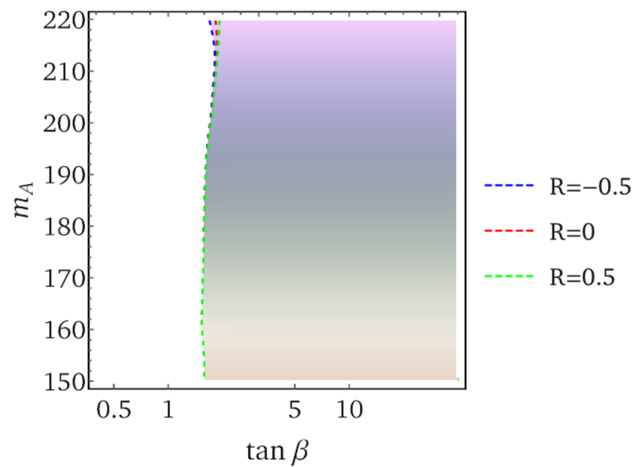
(a)

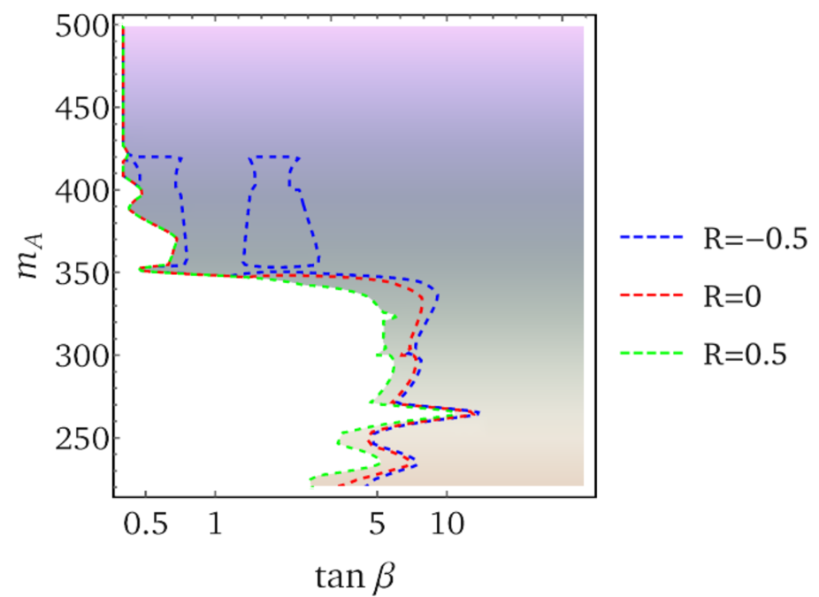
(b)

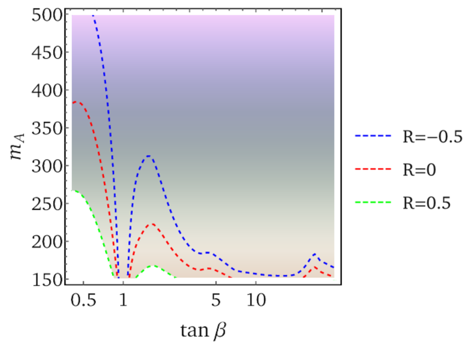
(c)

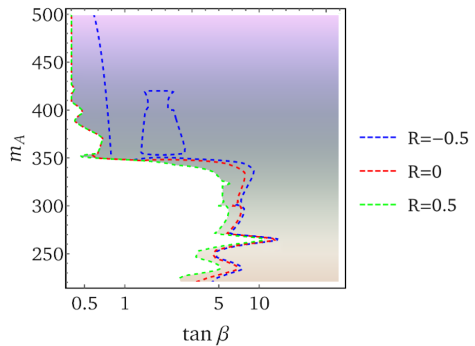
(d)

Figure 1: Bounds for Type-I Yukawa couplings. Regions ruled out by (a) $A/H\rightarrow\tau\tau$ data, (b) combination of collider constraints, including $A/H\rightarrow\tau\tau$, (c) precision Higgs global fits, and (d) combination of collider bounds and global fits of Higgs precision data. Each panel shows three different $R$ curves; the white regions of the parameter space are ruled out. In panels (b)–(d) the ruled out areas expand somewhat as $R$ decreases, with the borders of the allowed shaded regions indicated by the corresponding contours. For $R=-0.5$, the area enclosed by the closed dashed blue contour in panels (b) and (d) is also ruled out. There is a different $m_{A}$ scale in panel (a) as compared to the other three panels because the $A\rightarrow\gamma\gamma$ and $A\rightarrow Zh$ bounds are restricted to $m_{A}\mathrel{\raise 1.1625pt\hbox{$>$\kern-6.75pt\lower 3.87498pt\hbox{$\sim$}}}220\leavevmode\nobreak\ $\mathrm{GeV}$$. The color of the shaded regions bounded by the outermost contour in all figures is chosen solely for its aesthetic allure.

We now investigate the allowed parameter space taking into account collider, Higgs precision, and fine-tuning constraints—described in the previous two subsections. Amongst these, collider constraints, based on 95% CL limits on the cross section times branching ratio of the new heavy scalar states, depend on whether we employ a Type-I or a Type-II model, whereas tuning constraints are quite insensitive to this choice. Therefore it is natural to assess the impact of the two types of constraints separately. Figs. 1 and 2 show the parameter space allowed by collider constraints, whereas Figs. 3 and 4 show the tuning. The combined effects of these constraints are exhibited in Figs. 5 and 6. The special case of $R=1$ is presented in Fig. 7. Finally, we provide a rough projection of the anticipated sensitivity of the High Luminosity LHC to the parameter space of our model in Fig. 8. The color of the shaded regions bounded by the outermost contour in all figures is chosen solely for its aesthetic allure.

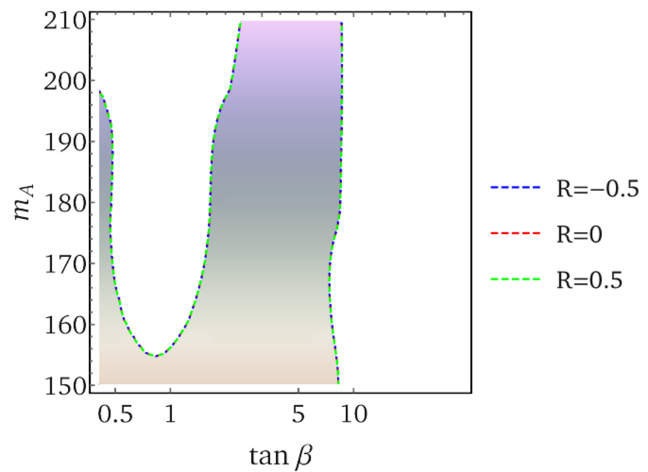
(a)

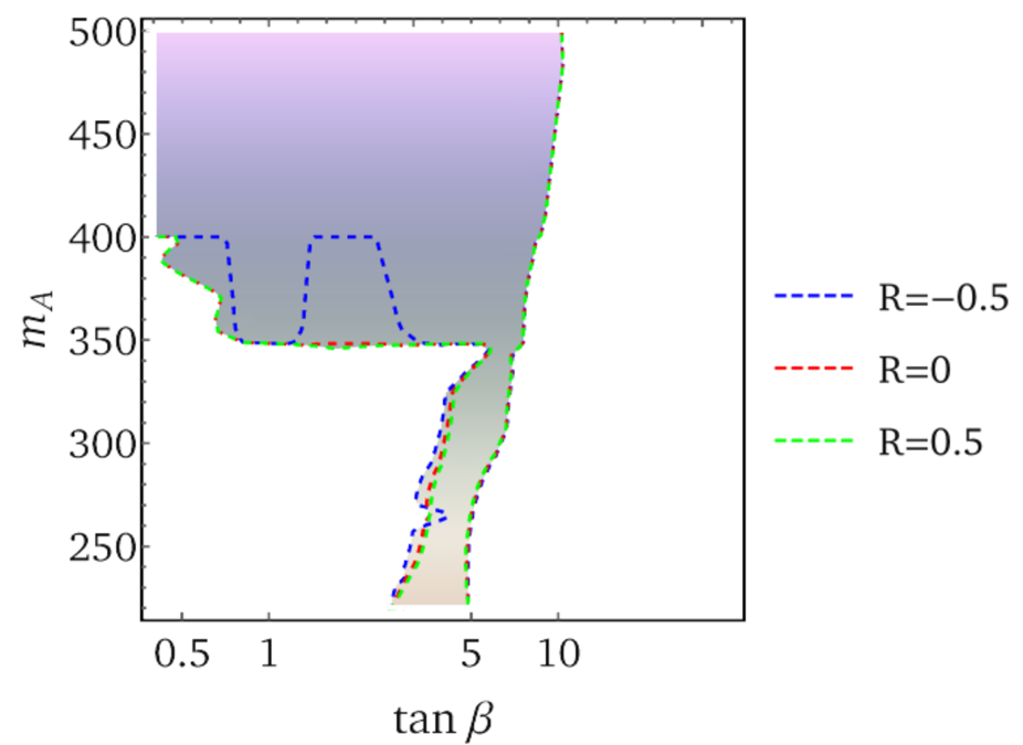
(b)

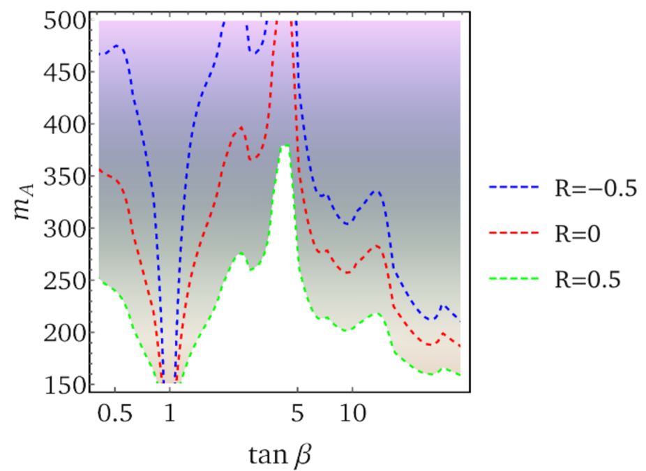
(c)

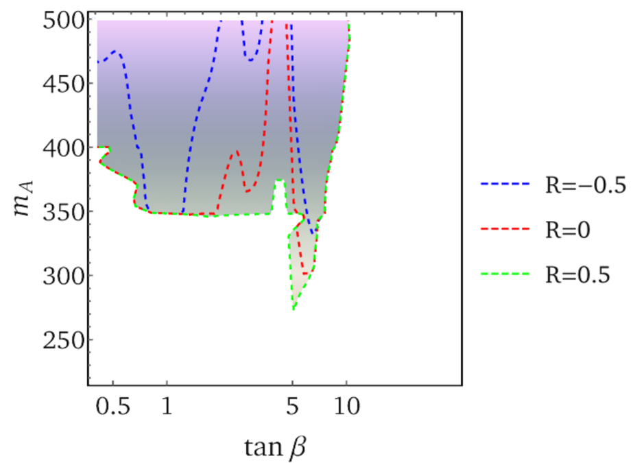
(d)

Figure 2: Bounds for Type-II Yukawa couplings. Regions ruled out by (a) $A/H\rightarrow\tau\tau$ data, (b) combination of collider constraints, including $A/H\rightarrow\tau\tau$, (c) precision Higgs global fits, and (d) combination of collider bounds and precision Higgs global fits. Each panel shows three different $R$ curves; the white regions of the parameter space are ruled out. In panels (b)–(d), the ruled out areas expand somewhat as $R$ decreases, with the borders of the allowed shaded regions indicated by the corresponding contours. There is a different $m_{A}$ scale in panel (a) as compared to the other three panels because the $A\rightarrow\gamma\gamma$ and $A\rightarrow Zh$ bounds are restricted to $m_{A}\mathrel{\raise 1.1625pt\hbox{$>$\kern-6.75pt\lower 3.87498pt\hbox{$\sim$}}}220\leavevmode\nobreak\ $\mathrm{GeV}$$.

The collider constraints shown in Figs. 1 and 2 are organized as follows: panel (a) shows the small-mass region—where $A\rightarrow Zh$ and $A\rightarrow\gamma\gamma$ are not relevant; panel (b) shows the combination of all considered collider constraints; panel (c) shows the parameter space ruled out from Higgs precision searches; and panel (d) shows the combination of collider and Higgs precision constraints. Note that the $m_{A}$ scale is different in Figs. 1(b) and 1(d).

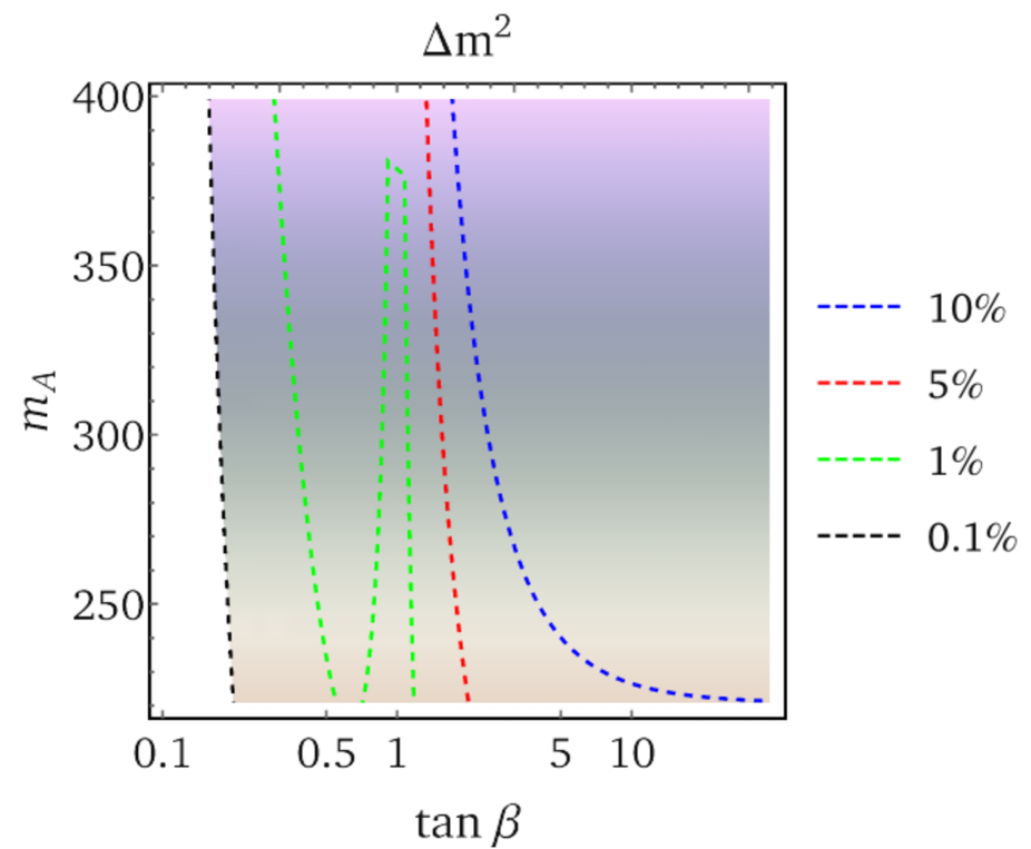
(a)

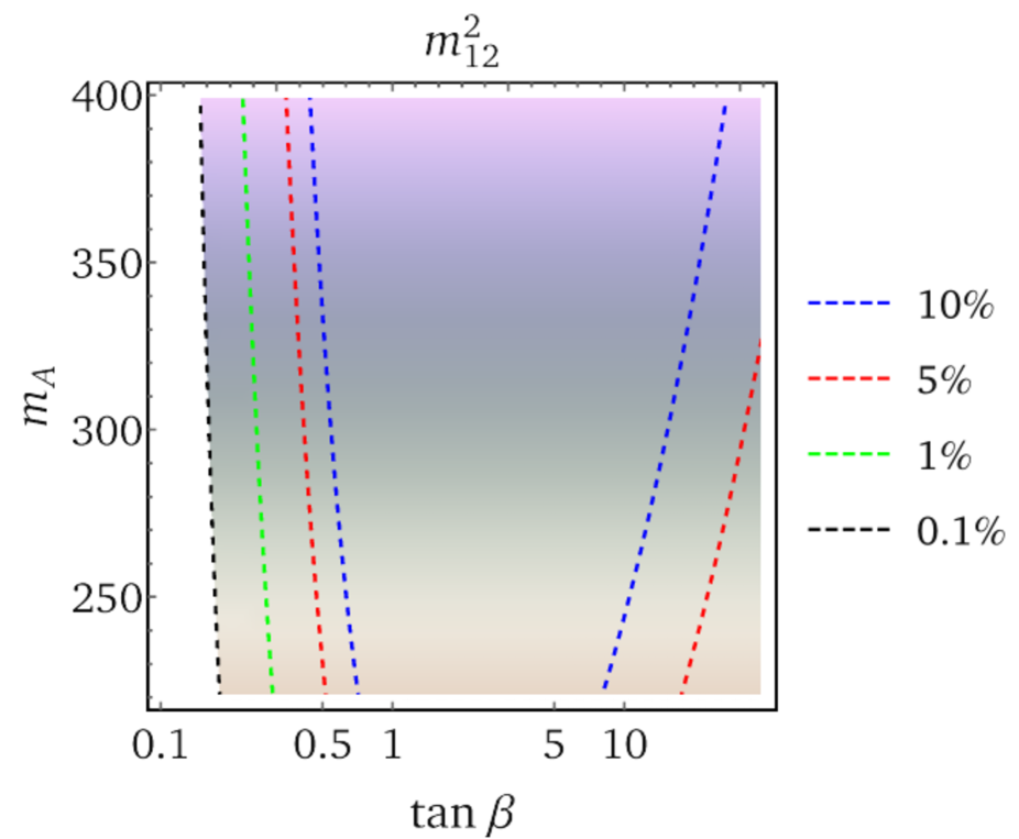
(b)

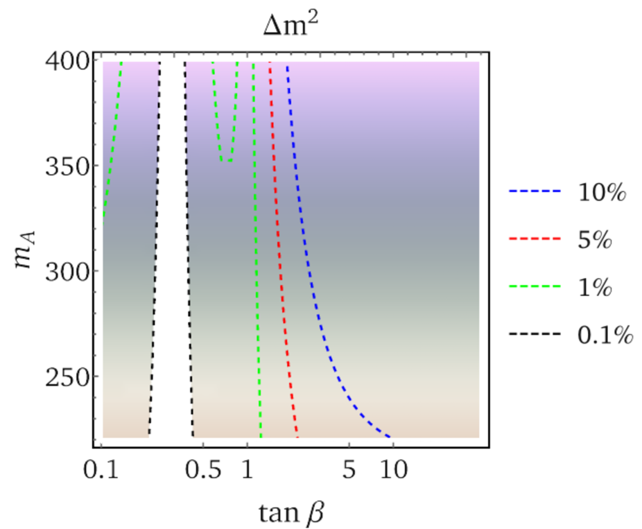
(c)

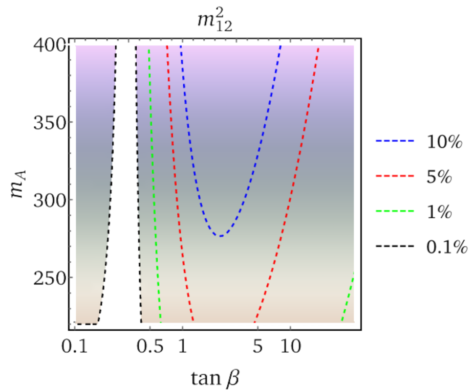
(d)

Figure 3: Contours of fine-tuning as defined in eq. (4.61). Panels (a) and (b) employ the benchmark points $R=0$ and $\gamma=0.1$, whereas panels (c) and (d) employ the benchmark points $R=0$ and $\gamma=0.3$. The shaded region inside and/or above each respective contour satisfies the corresponding tuning constraint.

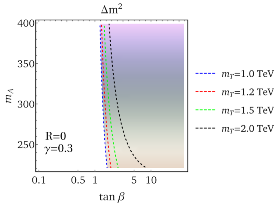
(a)

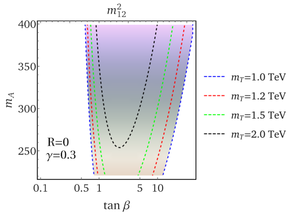
(b)

Figure 4: Dependence of the degree of fine-tuning for various masses of the vector-like top quark partner. The shaded region inside and/or above each respective contour corresponds to a fine-tuning of at most $5\%$. Both panels employ the benchmark points $R=0$ and $\gamma=0.3$.

Fig. 1(a) shows that the $A/H\rightarrow\tau\tau$ channel only restricts small $\tan\beta$ values for the Type-I model. This is expected because the production cross-section rapidly decreases as $\tan\beta\rightarrow\infty$. Other collider searches rule out a sizeable chunk of the low $\tan\beta$ parameter space as seen in Fig. 1(b). The weak dependence of collider bounds on $R$ is not shared by the fits to the Higgs precision data. Fig. 1(c) shows that larger $R$ values are less constrained than smaller ones. This behavior follows from eq. (3.19), as does the behavior as $\beta\rightarrow\frac{1}{4}\pi$ and $\beta\rightarrow\tfrac{1}{2}\pi$. The combination of these constraints, in Fig. 1(d), show that there is plenty of available parameter space at large $\tan\beta$ for the Type-I scenario, even for the smaller values of $m_{A}$.

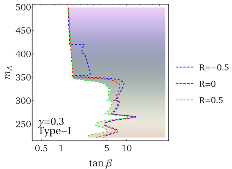
(a)

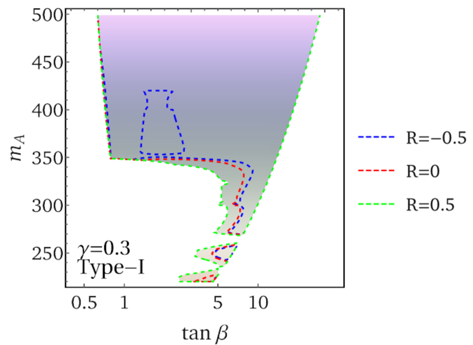
(b)

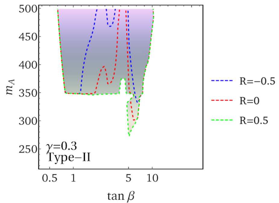
(c)

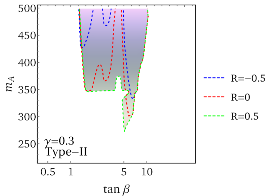
(d)

Figure 5: Experimental and tuning bounds for different $R$ values. The allowed shaded regions inside and/or above each respective contour satisfy all experimental bounds in addition to exhibiting a tuning of at most $5\%$ in $\Delta m^{2}$ (left) and $m_{12}^{2}$ (right). Panels (a) and (b) show the results for Type-I Yukawa couplings, and panels (c) and (d) show the results for Type-II Yukawa couplings. All panels employ the $\gamma=0.3$ benchmark.

The picture is rather different for the Type-II model. The $A/H$ production cross section rises for larger values of $\tan\beta$, and the $A/H\rightarrow\tau\tau$ branching sinks for small $\tan\beta$. This behavior, together with the lepton branching ratios, is reflected in Fig. 2(a), where the lepton decay channel mainly constrains large $\tan\beta$ values. Nevertheless, Fig. 2(b) shows that the small $\tan\beta$ region is almost entirely ruled by the $A\rightarrow\gamma\gamma$ and $A\rightarrow Zh$ channels. Higgs precision constraints rule out another chunk of parameter space. This is because Higgs precision data force Type-II close to exact Higgs alignment [$\cos(\beta-\alpha)\approx 0$], which is reflected by the strong $R$ dependence. Indeed, eq. (3.19) implies that $\cos(\beta-\alpha)\to 0$ in the limit of $R\rightarrow 1$. All these constraints are combined in Fig. 2(d) which shows, in combination with Fig. 7, that a light CP-odd scalar ($m_{A}\leq 350\leavevmode\nobreak\ $\mathrm{GeV}$$) is only possible for $R$ values close to $1$.

Moreover, it is noteworthy that all collider bounds are less severe for $m_{A}\geq 350\leavevmode\nobreak\ $\mathrm{GeV}$$. This is because the production cross-section drops for energies larger than the two-top-quark threshold. In addition, the area enclosed by the blue dotted line in figures 1(b), 1(d), and 2(b) comes from the $A\rightarrow Zh$ bound; the branching ratio vanishes for $\tan\beta=1$, and the $A\rightarrow Zh$ branching ratio is larger for smaller $R$.

Let us now turn to the degree of fine-tuning. Fig. 3 shows the fine-tuning measures as defined in eq. (4.61) for $\gamma=0.1$ and $\gamma=0.3$ and Fig. 4 shows the tuning for different $m_{T}$ values. The two tuning measures are complementary: $\Delta m^{2}$ mainly constrains small and intermediate $\tan\beta$ values, while $m^{2}_{12}$ constrains small and large $\tan\beta$. Note that the white regions in Fig. 3 occur when $\beta=\gamma$; that is, at $\beta=0.1$ in Figs. 3(a) and 3(b), and at $\beta=0.3$ in Figs. 3(c) and 3(d). This behavior can be traced back to eq. (4.50), and corresponds to the $y_{t}\rightarrow\infty$ limit. In addition, there is a region close to $\beta=\frac{1}{4}\pi$ where $\Delta m^{2}$ vanishes. This region is quite narrow and is indistinguishable in the figures. Of the two tunings, $m_{12}^{2}$ depends more strongly on $\gamma$ than $\Delta m^{2}$, as discussed in Section 4.5. Moreover, the $m_{T}$ dependence of the tunings is more pronounced for $m_{12}^{2}$ than for $\Delta m^{2}$ as shown in Fig. 4.

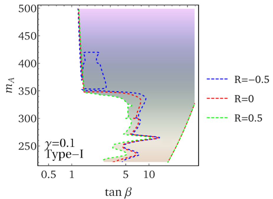
(a)

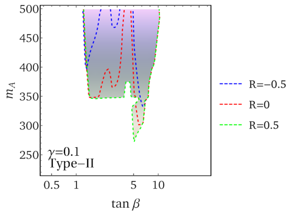
(b)

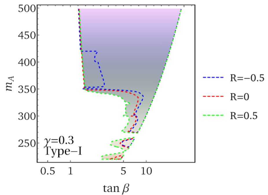
(c)

(d)

Figure 6: Regions allowed by experimental bounds and tuning constraints for different $R$, with an $m_{12}^{2}$ and $\Delta m^{2}$ tuning of at most $5\%$. Each panel shows three different $R$ curves; the white regions of the parameter space are ruled out. The ruled out areas expand somewhat as $R$ decreases, with the borders of the allowed shaded regions indicated by the corresponding contours. For $R=-0.5$, the area enclosed by the closed dashed blue contour in panel (a) is also ruled out. Panels (a) and (c) correspond to Type-I Yukawa couplings, and panels (b) and (d) correspond to Type-II Yukawa couplings. Panels (a) and (b) employ the $\gamma=0.1$ benchmark, whereas panels (c) and (d) employ $\gamma=0.3$.

Figs. 5 and 6 show the combination of collider and tuning constraints. Fig. 5(a), for Type-I, and Fig. 5(c), for Type-II, allow a $\Delta m^{2}$ tuning of at most $5\%$ and take into account collider constraints. Likewise, Figs. 5(b) and 5(d) are defined analogously and allow a tuning of $m_{12}^{2}$ of at most $5\%$. Both the $\Delta m^{2}$ and $m_{12}^{2}$ tuning constraints are combined in Fig. 6(c) for Type-I, and Fig. 6(d) for Type-II. These figures show that tuning constrains a region of parameter space untouched by other constraints. Of the two tuning measures, the $m_{12}^{2}$ tuning measure is salient—it restricts the large $\tan\beta$ region that is otherwise unconstrained for Type-I, and likewise but to a smaller extent for Type-II. However, lowering $\gamma$ makes tuning constraints less pronounced, as shown in Figs. 5(c) and 5(d). In summary, tuning constraints are complementary to collider bounds in these models, and moreover are not optional, as the purpose of our models is precisely to achieve approximate Higgs alignment (without decoupling) with minimal tuning.

In Fig. 7, we exhibit the experimental and tuning bounds for $R=1$, corresponding to the softly-broken SO($3$)-symmetric 2HDM. The allowed parameter regions for Type-I [panels (a) and (c)] and Type-II [panels (b) and (d)] are exhibited for $\gamma=0.1$ and $0.3$, respectively. This limiting case provides the most robust example of approximate Higgs alignment without decoupling in our framework, with allowed parameter regimes with $m_{A}$ as low as $200\leavevmode\nobreak\ $\mathrm{GeV}$$.

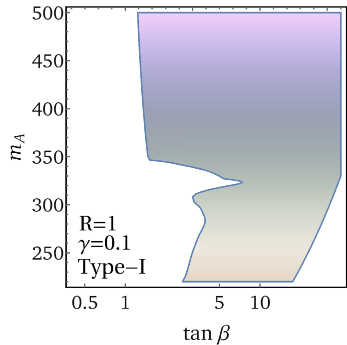
(a)

(b)

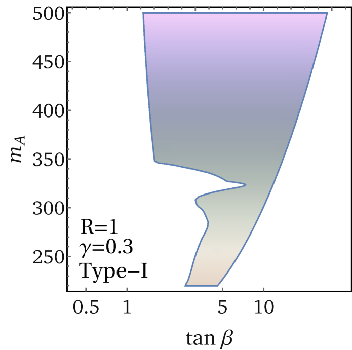
(c)

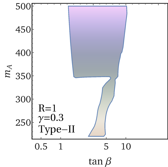
(d)

Figure 7: Experimental and tuning bounds for the softly-broken $\mathrm{SO}(3)$-symmetric 2HDM ($R=1$). The shaded regions in panels (a) and (b) satisfy all experimental bounds in addition to having a tuning of at most $5\%$ for both $\Delta m^{2}$ and $m_{12}^{2}$ in panels (c) and (d). Panels (a) and (c) correspond to Type-I Yukawa couplings, and panels (b) and (d) correspond to Type-II Yukawa couplings. Panels (a) and (b) employ the $\gamma=0.1$ benchmark, whereas panels (c) and (d) employ $\gamma=0.3$.

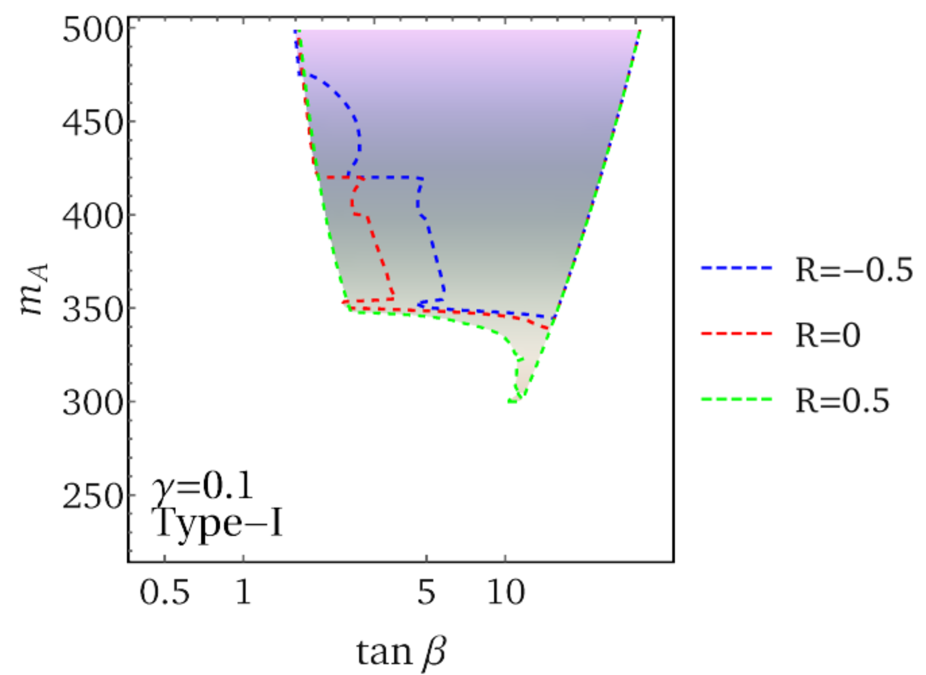
(a)

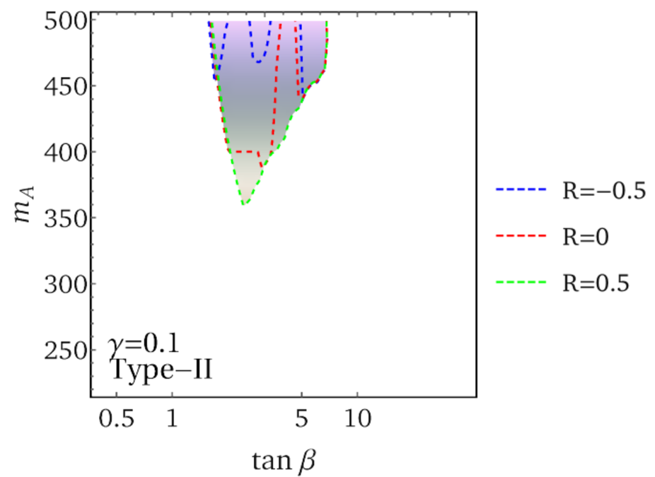
(b)

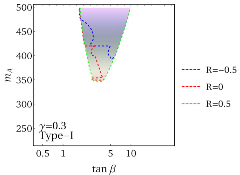
(c)

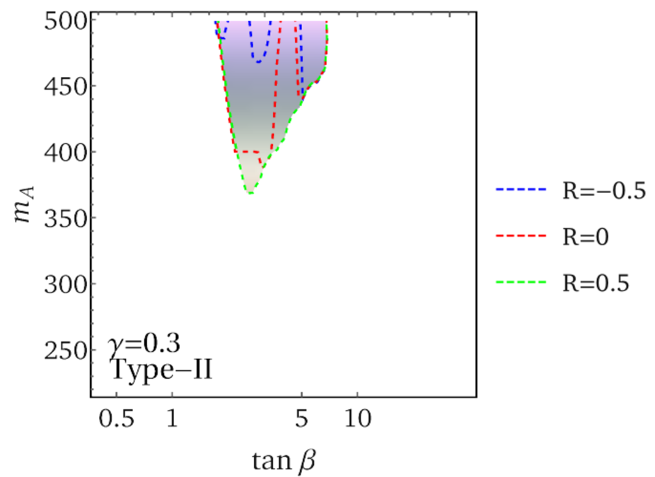
(d)

Figure 8: Projected regions allowed by experimental bounds anticipated at the high-luminosity LHC with $3000\leavevmode\nobreak\ $\mathrm{f}\mathrm{b}^{-1}$$ of data, assuming $m_{T}=2.5$ TeV with an $m_{12}^{2}$ and $\Delta m^{2}$ tuning of at most $5\%$. Each panel shows three different $R$ contours; the white regions of the parameter space are ruled out. The ruled out areas expand somewhat as $R$ decreases, with the borders of the allowed shaded regions indicated by the corresponding contours. Panels (a) and (c) correspond to Type-I Yukawa couplings, and panels (b) and (d) correspond to Type-II Yukawa couplings. Panels (a) and (b) employ the $\gamma=0.1$ benchmark, whereas panels (c) and (d) employ $\gamma=0.3$.

With the High-Luminosity LHC upgrade expected to begin taking data later in this decade, it is of interest to estimate the anticipated sensitivity to the parameter space of our model with $3000\leavevmode\nobreak\ $\mathrm{f}\mathrm{b}^{-1}$$ of data. First, the influx of data will likely tighten the bounds on vector-like quarks. To safely evade any new bounds (in the absence of a discovery) we increase the vector-like quark mass to $m_{T}=2.5\leavevmode\nobreak\ $\mathrm{TeV}$$. Second, we assume that all limits on experimental signal strengths for $H$ and $A$ production decrease by a factor of 4. The result of these considerations is shown in Fig. 8. The sub-plots of this figure are defined analogously to those of Fig. 6. As expected, the allowed parameter regions are severely reduced in Fig. 8 as compared to Fig. 6. Nonetheless, parameter space still exist where light scalar bosons ($\approx 350$ GeV) cannot be ruled out at the 95% CL. We also observe that the type-I results in Figs. 8(a) and 8(c) are quite sensitive to the value of $\gamma$. In particular, choosing a smaller $\gamma$ increases the allowed parameter space for larger $\tan\beta$ values. Furthermore, the allowed parameter space in the large $\tan\beta$ region increases for Type-I if one is willing to accept more fine-tuning. So it seems unlikely that the entire region of approximate Higgs alignment without decoupling can be ruled out for the Type-I scenario.

6 Conclusions

The 2HDM remains one of the simplest and best motivated extensions of the Standard Model. Theoretical and phenomenological studies of the 2HDM have been of great utility in guiding collider searches for new physics phenomena in the Higgs sector and have provided a useful framework for interpreting collider data.

Despite null results thus far from the LHC, the possibility of an extended Higgs sector remains viable. Of particular experimental interest is the case of approximate Higgs alignment without decoupling, where multiple states in the Higgs sector are light, but the neutral scalar interaction eigenstate, whose tree-level properties coincide with the SM Higgs field, does not mix strongly with the other scalar field degrees of freedom. If an approximate Higgs alignment is realized, then the present LHC Higgs data do not rule out this scenario, while the presence of other scalar states with masses not significantly larger than the electroweak scale and a small degree of mixing with the SM Higgs eigenstate provide experimental targets for the long-term LHC program.

In this work we have described an approximate global symmetry structure that results in approximate Higgs alignment. The global symmetry is one of the generalized CP symmetries of the 2HDM, and we extend it to the Yukawa sector by introducing vector-like fermions with soft symmetry-breaking masses. For practical purposes, a minimal addition of vector-like partners for the right-handed top quark is sufficient. The resulting model, although it does not address the ordinary electroweak hierarchy problem, realizes Higgs alignment without decoupling in an otherwise natural way. The structure in the Higgs sector, as well as the extended fermion sector, provide a range of collider signatures that can be accessed by future LHC searches.

We have assessed current experimental and fine-tuning constraints on the model parameters relevant for Higgs alignment arising from direct searches for vector-like top partners and new Higgs states, the LHC Higgs data, and precision electroweak observables. The model is viable and the new Higgs states can lie below about 500 GeV if the top partner is between one and a few TeV, $\tan\beta$ is in the range $\sim 1$–$10$, and the mixing between the top quark and the vector-like top partner is small. These restrictions are the result of an intricate interplay between experimental and tuning constraints. The viable parameter regimes provide attractive targets for the High-Luminosity LHC.

In addition to the generalized CP symmetry GCP$3$ employed in this work, there is another possible generalized CP symmetry of the 2HDM, GCP$2$, that can be used to impose Higgs alignment. Unlike the model studied here, softly breaking the GCP$2$ symmetry allows for the possibility of explicit and/or spontaneous CP violation in the Higgs sector Ferreira:2010hy . Further exploration of this model and its CP-violating phenomenology would be an interesting avenue for future work.

Appendix A Equivalence of the softly-broken GCP3 and U(1)$\otimes\Pi_{2}$ symmetric 2HDMs

To see that the softly-broken $\mathrm{U}(1)\otimes\Pi_{2}$-symmetric and GCP$3$-symmetric 2HDMs are in fact the same model expressed with respect to different scalar field bases Ferreira:2009wh , we provide the following details taken from Ref. Haber:2021zva . Consider the $\mathrm{U}(1)\otimes\Pi_{2}$ basis parameters with $\xi\neq 0$ and $m_{12}^{2}$ complex [subject to eq. (3.4)]. For convenience, we shall refrain from rephasing the scalar doublet fields to remove the phase $\xi$. Applying the following unitary transformation,

$$\Phi^{\prime}_{a}=U_{ab}\Phi_{b}\,,\quad\text{where $U=\frac{1}{\sqrt{2}}\begin{pmatrix}\phantom{-}1&-i\\ -i&\phantom{-}1\end{pmatrix}$}\,,$$ (A.1)

to the $\mathrm{U}(1)\otimes\Pi_{2}$ basis parameters yields the corresponding GCP$3$ basis parameters (denoted with prime superscripts),

$$\lambda^{\prime} = \tfrac{1}{2}\lambda(1+R)\,,$$ (A.2)

$$\lambda_{3}^{\prime} = \lambda_{3}+\tfrac{1}{2}\lambda(1-R)\,,$$ (A.3)

$$\lambda_{4}^{\prime} = \lambda_{4}+\tfrac{1}{2}\lambda(1-R)\,,$$ (A.4)

$$\lambda_{5}^{\prime} = -\tfrac{1}{2}\lambda(1-R)\,,$$ (A.5)

$$\lambda_{6}^{\prime} = -\lambda_{7}^{\prime}=0\,.$$ (A.6)

In particular, $\lambda_{5}^{\prime}=\lambda_{1}^{\prime}-\lambda_{3}^{\prime}-\lambda_{4}^{\prime}$ is real and $\lambda_{6}^{\prime}=\lambda_{7}^{\prime}=0$, corresponding to the GCP$3$ basis defined in Table 3.

In addition, the corresponding soft-breaking squared-mass parameters are,

$$m^{\prime\,2}_{11}=\tfrac{1}{2}(m_{11}^{2}+m_{22}^{2})+\operatorname{Im}m_{12}^{2}\,,$$ (A.7)

$$m^{\prime\,2}_{22}=\tfrac{1}{2}(m_{11}^{2}+m_{22}^{2})-\operatorname{Im}m_{12}^{2}\,,$$ (A.8)

$$m^{\prime\,2}_{12}=\operatorname{Re}m_{12}^{2}+\tfrac{1}{2}i(m_{22}^{2}-m_{11}^{2})\,.$$ (A.9)

Finally, the complex vevs in the GCP$3$ basis are given by

$$v_{1}^{\prime}=\frac{1}{\sqrt{2}}\bigl{(}v_{1}-iv_{2}e^{i\xi}\bigr{)}\,,\qquad\quad v_{2}^{\prime}=-\frac{i}{\sqrt{2}}\bigl{(}v_{1}+iv_{2}e^{i\xi}\bigr{)}\,.$$ (A.10)

Hence,

$$\tan^{2}\beta^{\prime}=\left|\frac{v_{2}^{\prime}}{v_{1}^{\prime}}\right|^{2}=\frac{v_{1}^{2}+v_{2}^{2}-2v_{1}v_{2}\sin\xi}{v_{1}^{2}+v_{2}^{2}+2v_{1}v_{2}\sin\xi}=\frac{1-s_{2\beta}\sin\xi}{1+s_{2\beta}\sin\xi}\,.$$ (A.11)

which implies that

$$s_{2\beta^{\prime}}^{2}=1-s_{2\beta}^{2}\sin^{2}\xi\,,$$ (A.12)

where $s_{2\beta^{\prime}}\equiv\sin 2\beta^{\prime}$ following our usual notation for sines and cosines. By convention, $0\leq\beta^{\prime}\leq\tfrac{1}{2}\pi$ (or equivalently, $\sin 2\beta^{\prime}\geq 0$).

The relative phase of the vevs in the GCP$3$ basis, denoted by $\xi^{\prime}$, is given by,

$$e^{i\xi^{\prime}}\tan\beta^{\prime}\equiv\frac{v_{2}^{\prime}}{v_{1}^{\prime}}=\frac{-iv_{1}+v_{2}e^{i\xi}}{v_{1}-iv_{2}e^{i\xi}}$$ (A.13)

Hence, we obtain,

$$e^{i\xi^{\prime}}=\frac{s_{2\beta}\cos\xi-ic_{2\beta}}{(1-s_{2\beta}^{2}\sin^{2}\xi)^{1/2}}\,.$$ (A.14)

That is,

$$\sin\xi^{\prime}=\frac{-c_{2\beta}}{(1-s_{2\beta}^{2}\sin^{2}\xi)^{1/2}}\,,\qquad\quad\cos\xi^{\prime}=\frac{s_{2\beta}\cos\xi}{(1-s_{2\beta}^{2}\sin^{2}\xi)^{1/2}}\,.$$ (A.15)

Hence eqs. (A.12) and (A.15) yield,

$$s_{2\beta^{\prime}}\sin\xi^{\prime}=-c_{2\beta}\,.$$ (A.16)

It is straightforward to verify that one obtains the same mass spectrum when computed in either scalar field basis. For example, in the ${\rm U}(1)\otimes\Pi_{2}$ basis, we have

$$m_{A}^{2}=\frac{2\operatorname{Re}(m_{12}^{2}e^{i\xi})}{s_{2\beta}}\,,$$ (A.17)

prior to a rephasing of the scalar fields to set $\xi=0$ [cf. eq. (3.13)]. To obtain $m_{A}^{2}$ expressed in terms of GCP$3$ basis parameters, we first employ eqs. (A.9), (A.12) and (A.14) to obtain

$$\frac{2\operatorname{Re}(m_{12}^{\prime\,2}e^{i\xi^{\prime}})}{s_{2\beta^{\prime}}}=\frac{2\operatorname{Re}(m_{12}^{2})s_{2\beta}\cos\xi+c_{2\beta}(m_{22}^{2}-m_{11}^{2})}{1-s_{2\beta}^{2}\sin^{2}\xi}\,.$$ (A.18)

In light of eq. (3.4), it follows that

$$\operatorname{Re}(m_{12}^{2})=\operatorname{Re}(m_{12}^{2}e^{i\xi})\cos\xi+\operatorname{Im}(m_{12}^{2}e^{i\xi})\sin\xi=\operatorname{Re}(m_{12}^{2}e^{i\xi})\cos\xi\,.$$ (A.19)

Hence, after using eqs. (3.2) and (3.3) to evaluate $m_{22}^{2}-m_{11}^{2}$, it follows that eq. (A.18) yields,

$$\frac{2\operatorname{Re}(m_{12}^{\prime\,2}e^{i\xi^{\prime}})}{s_{2\beta^{\prime}}}=\frac{2\operatorname{Re}(m_{12}^{2}e^{i\xi})}{s_{2\beta}}+\frac{\lambda v^{2}(1-R)c_{2\beta}^{2}}{2(1-s_{2\beta}^{2}\sin^{2}\xi)}\,.$$ (A.20)

Finally, using eq. (A.17), we end up with

$$m_{A}^{2}=\frac{2\operatorname{Re}(m_{12}^{\prime\,2}e^{i\xi^{\prime}})}{s_{2\beta^{\prime}}}+\lambda_{5}^{\prime}v^{2}\sin^{2}\xi^{\prime}\,,$$ (A.21)

after employing eqs. (A.5) and (A.15). Indeed, one can derive eq. (A.21) directly from the scalar potential expressed in terms of the GCP$3$ basis parameters, as expected. We have similarly verified that the masses of the other Higgs scalars computed in the GCP$3$ basis match those obtained in the $\mathrm{U}(1)\otimes\Pi_{2}$ basis.

As a final check of our computations, one can verify that $Y_{2}$, $Z_{1},\ldots,Z_{4}$, $|Z_{5}|$, $|Z_{6}|$, and $Z_{5}^{*}Z_{6}^{2}$ are invariant quantities that are independent of the choice of the scalar field basis. For example, starting from the GCP$3$ basis and transforming to the Higgs basis,

$$Z_{5}=\lambda_{5}^{\prime}e^{-2i\xi^{\prime}}\bigl{(}\cos\xi^{\prime}+ic_{2\beta^{\prime}}\sin\xi^{\prime}\bigr{)}^{2}\,,$$ (A.22)

$$Z_{6}=-Z_{7}=i\lambda_{5}^{\prime}s_{2\beta^{\prime}}\sin\xi^{\prime}e^{-i\xi^{\prime}}\bigl{(}\cos\xi^{\prime}+ic_{2\beta^{\prime}}\sin\xi^{\prime}\bigr{)}\,.$$ (A.23)

Note that CP is conserved in light of the relation,

$$Z^{2}_{6}=-\lambda_{5}^{\prime}s^{2}_{2\beta^{\prime}}\sin^{2}\xi^{\prime}Z_{5}\,,$$ (A.24)

which implies that $\operatorname{Im}(Z_{5}^{*}Z_{6}^{2})=0$. Hence, eqs. (A.22) and (A.24) yield,

$$Z_{5}^{*}Z_{6}^{2}=-\lambda_{5}^{\prime\,3}s_{2\beta^{\prime}}^{2}\sin^{2}\xi^{\prime}(1-s_{2\beta^{\prime}}^{2}\sin^{2}\xi^{\prime})^{2}=\tfrac{1}{8}\lambda^{3}(1-R)^{3}c_{2\beta}^{2}s^{4}_{2\beta}\,,$$ (A.25)

in agreement with eqs. (3.10) and (3.11). One can check that all the other invariant quantities also yield the same values in the GCP$3$ and $\mathrm{U}(1)\otimes\Pi_{2}$ basis.

Likewise, one can invert the transformations above and obtain the $\mathrm{U}(1)\otimes\Pi_{2}$ basis parameters starting from the GCP$3$ basis parameters. For completeness, these results are summarized below. First, the coefficients of the quartic terms of the scalar potential are given by,

$$\lambda = \lambda^{\prime}-\lambda_{5}^{\prime}\,,$$ (A.26)

$$\lambda_{3} = \lambda_{3}^{\prime}+\lambda_{5}^{\prime}\,,$$ (A.27)

$$\lambda_{4} = \lambda_{4}^{\prime}+\lambda_{5}^{\prime}\,,$$ (A.28)

$$\lambda R = \lambda^{\prime}+\lambda_{5}^{\prime}\,,$$ (A.29)

$$\lambda_{5} = \lambda_{6}=\lambda_{7}=0\,.$$ (A.30)

Next, the corresponding soft-breaking squared-mass parameters are:

$$m^{2}_{11}=\tfrac{1}{2}(m_{11}^{\prime\,2}+m_{22}^{\prime\,2})-\operatorname{Im}m_{12}^{\prime\,2}\,,$$ (A.31)

$$m^{2}_{22}=\tfrac{1}{2}(m_{11}^{\prime\,2}+m_{22}^{\prime\,2})+\operatorname{Im}m_{12}^{\prime\,2}\,,$$ (A.32)

$$m^{2}_{12}=\operatorname{Re}m_{12}^{\prime\,2}-\tfrac{1}{2}i(m_{22}^{\prime\,2}-m_{11}^{\prime\,2})\,.$$ (A.33)

Finally, the complex vevs in the $\mathrm{U}(1)\otimes\Pi_{2}$ basis are given by

$$v_{1}=\frac{1}{\sqrt{2}}\bigl{(}v^{\prime}_{1}+iv^{\prime}_{2}e^{i\xi^{\prime}}\bigr{)}\,,\qquad\quad v_{2}^{\prime}=\frac{i}{\sqrt{2}}\bigl{(}v^{\prime}_{1}-iv^{\prime}_{2}e^{i\xi^{\prime}}\bigr{)}\,.$$ (A.34)

Hence,

$$\tan^{2}\beta=\left|\frac{v_{2}}{v_{1}}\right|^{2}=\frac{v_{1}^{\prime\,2}+v_{2}^{\prime\,2}+2v_{1}v_{2}\sin\xi}{v_{1}^{\prime\,2}+v_{2}^{\prime\,2}-2v_{1}v_{2}\sin\xi}=\frac{1+s_{2\beta^{\prime}}\sin\xi^{\prime}}{1-s_{2\beta^{\prime}}\sin\xi^{\prime}}\,.$$ (A.35)

which implies that

$$s_{2\beta}^{2}=1-s_{2\beta^{\prime}}^{2}\sin^{2}\xi^{\prime}\,.$$ (A.36)

The relative phase of the vevs in the U(1)$\otimes\Pi_{2}$ basis, denoted by $\xi$, is given by,

$$\sin\xi=\frac{c_{2\beta^{\prime}}}{(1-s_{2\beta^{\prime}}^{2}\sin^{2}\xi^{\prime})^{1/2}}\,,\qquad\quad\cos\xi=\frac{s_{2\beta^{\prime}}\cos\xi^{\prime}}{(1-s_{2\beta^{\prime}}^{2}\sin^{2}\xi^{\prime})^{1/2}}\,,\qquad\quad$$ (A.37)

Hence eqs. (A.36) and (A.37) yield,

$$s_{2\beta}\sin\xi=c_{2\beta^{\prime}}\,.$$ (A.38)

Of course, once the $\mathrm{U}(1)\otimes\Pi_{2}$ basis parameters have been derived, one can perform one further rephasing to remove the complex phase $\xi$ (thereby setting $\xi=0$).

Appendix B Singular value decomposition of a real $2\times 2$ matrix

The material presented in this Appendix is taken from Ref. Haber:2020wco .

For any real $n\times n$ matrix $M$, real orthogonal $n\times n$ matrices $L$ and $R$ exist such that

$$L^{{\mathsf{T}}}MR=M_{D}={\rm diag}(m_{1},m_{2},\ldots,m_{n}),$$ (B.1)

where the $m_{k}$ are real and nonnegative. This corresponds to the singular value decomposition of $M$ restricted to the space of real matrices.

The singular value decomposition of a general $2\times 2$ real matrix can be performed fully analytically. Let us consider the non-diagonal real matrix,

$$M=\left(\begin{array}[]{cc}a&\quad c\\ \tilde{c}&\quad b\end{array}\right)\,,$$ (B.4)

where at least one of the two quantities $c$ or $\tilde{c}$ is non-vanishing. The real singular value decomposition of $M$ is

$$L^{{\mathsf{T}}}MR=\begin{pmatrix}m_{1}&\,\,\,0\\ 0&\,\,\,m_{2}\end{pmatrix}\,,$$ (B.5)

where $L$ and $R$ are real $2\times 2$ orthogonal matrices and $m_{1}$ and $m_{2}$ are nonnegative. In general, one can parameterize $L$ and $R$ in eq. (B.5) by

$$L=\left(\begin{array}[]{cc}\phantom{-}\cos\theta_{L}&\sin\theta_{L}\\ -\sin\theta_{L}&\cos\theta_{L}\end{array}\right)\begin{pmatrix}1&\,\,\,0\\ 0&\,\,\,\varepsilon_{L}\end{pmatrix}\,,\qquad\quad R=\left(\begin{array}[]{cc}\phantom{-}\cos\theta_{R}&\sin\theta_{R}\\ -\sin\theta_{R}&\cos\theta_{R}\end{array}\right)\begin{pmatrix}1&\,\,\,0\\ 0&\,\,\,\varepsilon_{R}\end{pmatrix}\,,$$ (B.6)

where $-\tfrac{1}{2}\pi<\theta_{L,R}\leq\tfrac{1}{2}\pi$, and $\varepsilon_{L,R}=\pm 1$. Note that $\det L=\varepsilon_{L}$ and $\det R=\varepsilon_{R}$, which implies that $\varepsilon_{L}\varepsilon_{R}\det M=m_{1}m_{2}$. Since $m_{1}$, $m_{2}\geq 0$, it follows that $\operatorname{sgn}(\det M)=\varepsilon_{L}\varepsilon_{R}$. Thus, only the product of $\varepsilon_{L}$ and $\varepsilon_{R}$ is fixed by eq. (B.5).

The diagonal elements of $L^{{\mathsf{T}}}MR$ can be determined by taking the positive square root of the nonnegative eigenvalues, $m^{2}_{1,2}$, of the real orthogonal matrix $M^{{\mathsf{T}}}M$,

$$m^{2}_{1,2}=\tfrac{1}{2}\bigl{[}a^{2}+b^{2}+c^{2}+\tilde{c}^{2}\mp\Delta\bigr{]}\,,$$ (B.7)

in a convention where $0\leq m_{1}\leq m_{2}$ (i.e., $\Delta\geq 0$), with

$$\Delta \equiv \bigl{[}(a^{2}-b^{2}-c^{2}+\tilde{c}^{2})^{2}+4(ac+b\tilde{c})^{2}\bigr{]}^{1/2}$$ (B.8)

$$= \bigl{[}(a^{2}+b^{2}+c^{2}+\tilde{c}^{2})^{2}-4(ab-c\tilde{c})^{2}\bigr{]}^{1/2}\,.$$

Note that

$$m_{1}^{2}+m_{2}^{2}=a^{2}+b^{2}+c^{2}+\tilde{c}^{2}\,,\qquad\quad m_{1}m_{2}=\varepsilon_{L}\varepsilon_{R}(ab-c\tilde{c})\,.$$ (B.9)

Moreover, $m_{1}=m_{2}$ if and only if $a=\pm b$ and $c=\mp\tilde{c}$, which imply that $ac+b\tilde{c}=0$ and $\Delta=0$.

We first assume that $m_{1}\neq m_{2}$. Then, if we rewrite eq. (B.5) in the form $MR=LM_{D}$, where $M_{D}\equiv{\rm diag}(m_{1}\,,\,m_{2})$, then we immediately obtain,

$$m_{1}\cos\theta_{L} = a\cos\theta_{R}-c\sin\theta_{R}\,,\qquad\quad\varepsilon_{L}\varepsilon_{R}m_{2}\sin\theta_{L}=a\sin\theta_{R}+c\cos\theta_{R}\,,$$ (B.10)

$$m_{1}\sin\theta_{L} = b\sin\theta_{R}-\tilde{c}\cos\theta_{R}\,,\qquad\quad\,\varepsilon_{L}\varepsilon_{R}m_{2}\cos\theta_{L}=\tilde{c}\sin\theta_{R}+b\cos\theta_{R}\,.$$ (B.11)

It follows that

$$m_{1}^{2}\cos^{2}\theta_{L}+m_{2}^{2}\sin^{2}\theta_{L}=a^{2}+c^{2}\,,\qquad\quad m_{1}^{2}\sin^{2}\theta_{L}+m_{2}^{2}\cos^{2}\theta_{L}=b^{2}+\tilde{c}^{2}\,.$$ (B.12)

Subtracting these two equations, and employing eq. (B.8) yields,

$$\cos 2\theta_{L}=\frac{b^{2}-a^{2}-c^{2}+\tilde{c}^{2}}{\Delta}\,,\qquad\quad\cos 2\theta_{R}=\frac{b^{2}-a^{2}+c^{2}-\tilde{c}^{2}}{\Delta}\,.$$ (B.13)

In obtaining $\cos 2\theta_{R}$, it is sufficient to note that eqs. (B.10)–(B.12) are valid under the interchange of $c\leftrightarrow\tilde{c}$ and the interchange of the subscripts $L\leftrightarrow R$.

We can also use eqs. (B.10) and (B.11) to obtain,

$$m_{1}^{2}\cos\theta_{L}\sin\theta_{L}=(a\cos\theta_{R}-c\sin\theta_{R})(b\sin\theta_{R}-\tilde{c}\cos\theta_{R})\,,$$ (B.14)

$$m_{2}^{2}\cos\theta_{L}\sin\theta_{L}=(a\sin\theta_{R}+c\cos\theta_{R})(\tilde{c}\sin\theta_{R}+b\cos\theta_{R})\,.$$ (B.15)

Subtracting these two equations yields

$$\sin 2\theta_{L}=\frac{2(a\tilde{c}+bc)}{\Delta}\,,\qquad\quad\sin 2\theta_{R}=\frac{2(ac+b\tilde{c})}{\Delta}\,,$$ (B.16)

after again noting the symmetry under $c\to\tilde{c}$ and the interchange of the subscripts $L\leftrightarrow R$.

Thus, employing eqs. (B.13) and (B.16), we have succeeded in uniquely determining the angles $\theta_{L}$ and $\theta_{R}$ (where $-\tfrac{1}{2}\pi<\theta_{L,R}\leq\tfrac{1}{2}\pi$). As noted below eq. (B.6), the individual signs $\varepsilon_{L}$ and $\varepsilon_{R}$ are not separately fixed (implying that one is free to set one of these two signs to $+1$); only the product $\varepsilon_{L}\varepsilon_{R}=\operatorname{sgn}(\det M)$ is determined by the singular value decomposition of $M$.

A useful identity can now be derived that exhibits a direct relation between the angles $\theta_{L}$ and $\theta_{R}$. First, we note two different trigonometric identities for the tangent function,

$$\tan\theta_{L} = \frac{1-\cos 2\theta_{L}}{\sin 2\theta_{L}}=\frac{m_{2}^{2}-m_{1}^{2}-b^{2}+a^{2}+c^{2}-\tilde{c}^{2}}{2(a\tilde{c}+bc)}=\frac{a^{2}+c^{2}-m_{1}^{2}}{a\tilde{c}+bc}\,,$$ (B.17)

$$\tan\theta_{R} = \frac{\sin 2\theta_{R}}{1+\cos 2\theta_{R}}=\frac{2(ac+b\tilde{c})}{m_{2}^{2}-m_{1}^{2}+b^{2}-a^{2}+c^{2}-\tilde{c}^{2}}=\frac{ac+b\tilde{c}}{m_{2}^{2}-a^{2}-\tilde{c}^{2}}\,,$$ (B.18)

where we have made use of eqs. (B.9), (B.13) and (B.16). It then follows that

$$\frac{\tan\theta_{L}}{\tan\theta_{R}}=\frac{(a^{2}+c^{2}-m_{1}^{2})(m_{2}^{2}-a^{2}-\tilde{c}^{2})}{(a\tilde{c}+bc)(ac+b\tilde{c})}\,.$$ (B.19)

The numerator of eq. (B.19) can be simplified with a little help from eq. (B.9) as follows,

$$(a^{2}+c^{2}-m_{1}^{2})(m_{2}^{2}-a^{2}-\tilde{c}^{2}) = a^{2}(m_{1}^{2}+m_{2}^{2})+c^{2}m_{2}^{2}-\tilde{c}^{2}m_{1}^{2}-(a^{2}+c^{2})(a^{2}+\tilde{c}^{2})-m_{1}^{2}m_{2}^{2}$$ (B.20)

$$= a^{2}(a^{2}+b^{2}+c^{2}+\tilde{c}^{2})-(a^{2}+c^{2})(a^{2}+\tilde{c}^{2})$$

$$\qquad\qquad+c^{2}m_{2}^{2}+\tilde{c}^{2}m_{1}^{2}-(ab-c\tilde{c})^{2}$$

$$= c^{2}m_{2}^{2}+\tilde{c}^{2}m_{1}^{2}+2(ab-c\tilde{c})c\tilde{c}=(cm_{2}+\varepsilon_{L}\varepsilon_{R}\tilde{c}m_{1})^{2}\,.$$

Likewise, the denominator of eq. (B.19) can be simplified as follows,

$$(a\tilde{c}+bc)(ac+b\tilde{c}) = (ab-c\tilde{c})(c^{2}+\tilde{c}^{2})+c\tilde{c}(a^{2}+b^{2}+c^{2}+\tilde{c}^{2})$$ (B.21)

$$= \varepsilon_{L}\varepsilon_{R}m_{1}m_{2}(c^{2}+\tilde{c}^{2})+c\tilde{c}(m_{1}^{2}+m_{2}^{2})$$

$$= (cm_{2}+\varepsilon_{L}\varepsilon_{R}\tilde{c}m_{1})(\tilde{c}m_{2}+\varepsilon_{L}\varepsilon_{R}cm_{1})\,.$$

Hence, we end up with a remarkably simple result,

$$\frac{\tan\theta_{L}}{\tan\theta_{R}}=\frac{cm_{2}+\varepsilon_{L}\varepsilon_{R}\tilde{c}m_{1}}{\tilde{c}m_{2}+\varepsilon_{L}\varepsilon_{R}cm_{1}}\,.$$ (B.22)

The case of $m_{1}=0$, which arises when $\det M=ab-c\tilde{c}=0$, is noteworthy. It then follows that $\Delta=(a^{2}+\tilde{c}^{2})(b^{2}+\tilde{c}^{2})/\tilde{c}^{2}$ [cf. eq. (B.8) with $c=ab/\tilde{c}$] and,

$$\tan\theta_{L}=\frac{a}{\tilde{c}}\,,\qquad\quad\tan\theta_{R}=\frac{\tilde{c}}{b}\,.$$ (B.23)

In particular, after using $ab=c\tilde{c}$, it follows that

$$\frac{\tan\theta_{L}}{\tan\theta_{R}}=\frac{c}{\tilde{c}}\,,\qquad\text{for $m_{1}=0$}.$$ (B.24)

This is indeed the correct limit of eq. (B.22) when $m_{1}=0$, as expected. In this case, the signs $\varepsilon_{L}$ and $\varepsilon_{R}$ are arbitrary, and one can choose $\varepsilon_{L}=\varepsilon_{R}=1$ without loss of generality.

For completeness, we note that the case of $m\equiv m_{1}=m_{2}\neq 0$ must be treated separately. In this case, $a=\pm b$ and $c=\mp\tilde{c}$, which yields $m=(a^{2}+c^{2})^{1/2}$. Since eq. (B.5) implies that $MR=mL$, one can take $R$ to be an arbitrary $2\times 2$ real orthogonal matrix. Using eq. (B.6), the matrix $L$ is now determined,

$$\cos\theta_{L}=\frac{a\cos\theta_{R}-c\sin\theta_{R}}{\sqrt{a^{2}+c^{2}}}\,,\qquad\quad\sin\theta_{L}=\pm\left(\frac{c\cos\theta_{R}+a\sin\theta_{R}}{\sqrt{a^{2}+c^{2}}}\right)\,,$$ (B.25)

subject to the constraint $\varepsilon_{L}\varepsilon_{R}=\pm 1$ that determines the sign factor appearing in the expression for $\sin\theta_{L}$ given in eq. (B.25).

Appendix C Top quark mixing revisited

In Sections 4.2 and 4.3, we determined the mixing of the top quark and its vector-like partners by a two step procedure. In the first step, the effects of electroweak symmetry breaking were ignored. The Yukawa interactions and mass terms were then obtained in terms of the mass eigenstate fields, $\bar{x}_{0}$ and $\overline{X}_{0}$, resulting in eq. (4.25). In the second step, the fields $\bar{x}_{0}$ and $\overline{X}_{0}$ were treated as interaction eigenstates, and the new mass eigenstates were determined when the Higgs field vevs are taken into account.

One could have performed the same analysis in one step by treating the effects of electroweak symmetry breaking from the beginning by employing $\Phi_{i}^{0}=v_{i}/\sqrt{2}+\overline{\Phi}_{i}^{\lower 3.0pt\hbox{$\scriptstyle 0$}}$ (for $i=1,2$) in eq. (4.15). In this case, the interaction eigenstates are given by $\hat{\chi}_{i}=(u\quad U)$ and $\hat{\eta}^{j}=(\bar{u}\quad\overline{U})$ as in Section 4.2, whereas the mass matrix given in eq. (4.21) is modified as follows,

$$\mathcal{M}=\begin{pmatrix}Ys_{\beta}&\,\,\,Yc_{\beta}\\ M_{u}&\,\,\,M_{U}\end{pmatrix}\,,$$ (C.1)

where $Y\equiv y_{t}v/\sqrt{2}$. Using the results of Appendix B, one can then directly determine the fermion masses and mixing.

As expected, eq. (B.7) yields the squared-masses of the two Dirac fermions previously given in eq. (4.42). The singular value decomposition of $\mathcal{M}$ [cf. eq. (C.1)] involves two mixing angles, denoted below by $\theta^{\prime}_{L}$ and $\theta^{\prime}_{R}$, that are given by

$$\sin 2\theta^{\prime}_{L} = \frac{2YMc_{\beta-\gamma}}{m_{T}^{2}-m_{t}^{2}}\,,\qquad\qquad\cos 2\theta^{\prime}_{L}=\frac{M^{2}-Y^{2}}{m_{T}^{2}-m_{t}^{2}}\,,$$ (C.2)

$$\sin 2\theta^{\prime}_{R} = \frac{Y^{2}s_{2\beta}+M^{2}s_{2\gamma}}{m_{T}^{2}-m_{t}^{2}}\,,\qquad\,\cos 2\theta^{\prime}_{R}=\frac{Y^{2}c_{2\beta}+M^{2}c_{2\gamma}}{m_{T}^{2}-m_{t}^{2}}\,,$$ (C.3)

which uniquely determine the mixing angles modulo $\pi$. Note that in addition to the mixing angles $\theta^{\prime}_{L}$ and $\theta^{\prime}_{R}$, the matrices $L$ and $R$ given in eq. (B.6) depend on $\varepsilon_{L}$ and $\varepsilon_{R}$, where $\varepsilon_{L}\varepsilon_{R}={\rm\operatorname{sgn}}(YMs_{\beta-\gamma})$, which is the same result obtained below eq. (4.45).

All the results of this Appendix could have been anticipated given that $\theta^{\prime}_{L}$ and $\theta^{\prime}_{R}$ are related to the mixing angles $\theta_{L}$ and $\theta_{R}$ of Section 4.3 as follows,

$$\theta^{\prime}_{L}=\theta_{L}\,,\qquad\quad\theta^{\prime}_{R}=\gamma+\theta_{R}\,.$$ (C.4)

Indeed, using eq. (C.4) and the results of eqs. (4.44) and (4.45), one can recover the expressions presented in eqs. (C.2) and (C.3). Finally, eqs. (4.47) and (C.4) yield,

$$\tan\theta^{\prime}_{L}=\varepsilon_{L}\varepsilon_{R}\frac{m_{T}}{m_{t}}\tan(\theta^{\prime}_{R}-\gamma)\,.$$ (C.5)

By employing the identities for the tangent function given in eqs. (B.17) and (B.18), one can derive eq. (C.5) directly starting from eqs. (C.2) and (C.3).

References

- (1) ATLAS Collaboration, G. Aad et al., “Observation of a new particle in the search for the Standard Model Higgs boson with the ATLAS detector at the LHC,” Phys. Lett. B 716 (2012) 1, arXiv:1207.7214 [hep-ex].
- (2) CMS Collaboration, S. Chatrchyan et al., “Observation of a New Boson at a Mass of GeV with the CMS Experiment at the LHC,” Phys. Lett. B 716 (2012) 30, arXiv:1207.7235 [hep-ex].
- (3) CMS Collaboration, A. M. Sirunyan et al., “Combined measurements of Higgs boson couplings in proton–proton collisions at ,” Eur. Phys. J. C 79 (2019) 421, arXiv:1809.10733 [hep-ex].
- (4) ATLAS Collaboration, G. Aad et al., “Combined measurements of Higgs boson production and decay using up to fb-1 of proton-proton collision data at TeV collected with the ATLAS experiment,” Phys. Rev. D 101 (2020) 012002, arXiv:1909.02845 [hep-ex].
- (5) CMS Collaboration, “Combined Higgs boson production and decay measurements with up to 137 fb-1 of proton-proton collision data at TeV,” CMS-PAS-HIG-19-005 (January, 2020) .
- (6) J. F. Gunion, H. E. Haber, G. L. Kane, and S. Dawson, The Higgs Hunter’s Guide. (Westview Press, Boulder, CO), 2000.
- (7) P. Fayet, “Supergauge Invariant Extension of the Higgs Mechanism and a Model for the electron and Its Neutrino,” Nucl. Phys. B 90 (1975) 104.
- (8) S. Dimopoulos and H. Georgi, “Softly Broken Supersymmetry and SU(),” Nucl. Phys. B 193 (1981) 150.
- (9) L. Susskind, “The Gauge Hierachy Problem, Technicolor, Supersymmetry, and all that.,” Phys. Rept. 104 (1984) 181.
- (10) G. C. Branco, P. M. Ferreira, L. Lavoura, M. N. Rebelo, M. Sher, and J. P. Silva, “Theory and phenomenology of two-Higgs-doublet models,” Phys. Rept. 516 (2012) 1, arXiv:1106.0034 [hep-ph].
- (11) N. Craig, J. Galloway, and S. Thomas, “Searching for Signs of the Second Higgs Doublet,” arXiv:1305.2424 [hep-ph].
- (12) H. E. Haber, “The Higgs data and the Decoupling Limit,” in st Toyama International Workshop on Higgs as a Probe of New Physics (HPNP) Toyama, Japan, February -, . arXiv:1401.0152 [hep-ph].
- (13) M. Carena, I. Low, N. R. Shah, and C. E. M. Wagner, “Impersonating the Standard Model Higgs Boson: Alignment without Decoupling,” JHEP 04 (2014) 015, arXiv:1310.2248 [hep-ph].
- (14) D. Asner, T. Barklow, C. Calancha, K. Fujii, N. Graf, et al., “ILC Higgs White Paper,” arXiv:1310.0763 [hep-ph]. See Chapter 1.3.
- (15) H. E. Haber and Y. Nir, “Multiscalar Models With a High-energy Scale,” Nucl. Phys. B335 (1990) 363.
- (16) J. F. Gunion and H. E. Haber, “The CP conserving two Higgs doublet model: The Approach to the decoupling limit,” Phys. Rev. D67 (2003) 075019, arXiv:hep-ph/0207010 [hep-ph].
- (17) E. Ma, “Verifiable radiative seesaw mechanism of neutrino mass and dark matter,” Phys. Rev. D 73 (2006) 077301, arXiv:hep-ph/0601225.
- (18) R. Barbieri, L. J. Hall, and V. S. Rychkov, “Improved naturalness with a heavy Higgs: An Alternative road to LHC physics,” Phys. Rev. D 74 (2006) 015007, arXiv:hep-ph/0603188.
- (19) P. S. Bhupal Dev and A. Pilaftsis, “Maximally Symmetric Two Higgs Doublet Model with Natural Standard Model Alignment,” JHEP 12 (2014) 024, arXiv:1408.3405 [hep-ph]. [Erratum: JHEP 11 (2015) 147].
- (20) A. Pilaftsis, “Symmetries for standard model alignment in multi-Higgs doublet models,” Phys. Rev. D93 (2016) 075012, arXiv:1602.02017 [hep-ph].
- (21) P. Draper, H. E. Haber, and J. T. Ruderman, “Partially Natural Two Higgs Doublet Models,” JHEP 06 (2016) 124, arXiv:1605.03237 [hep-ph].
- (22) P. M. Ferreira, H. E. Haber, and J. P. Silva, “Generalized CP symmetries and special regions of parameter space in the two-Higgs-doublet model,” Phys. Rev. D79 (2009) 116004, arXiv:0902.1537 [hep-ph].
- (23) R. D. Peccei and H. R. Quinn, “Constraints Imposed by CP Conservation in the Presence of Instantons,” Phys. Rev. D16 (1977) 1791.
- (24) P. Fayet, “A Gauge Theory of Weak and Electromagnetic Interactions with Spontaneous Parity Breaking,” Nucl. Phys. B 78 (1974) 14.
- (25) L. J. Hall and M. B. Wise, “Flavor changing Higgs-Boson Couplings,” Nucl. Phys. B 187 (1981) 397.
- (26) V. D. Barger, J. Hewett, and R. Phillips, “New Constraints on the Charged Higgs Sector in Two Higgs Doublet Models,” Phys. Rev. D 41 (1990) 3421.
- (27) M. Aoki, S. Kanemura, K. Tsumura, and K. Yagyu, “Models of Yukawa interaction in the two Higgs doublet model, and their collider phenomenology,” Phys. Rev. D 80 (2009) 015017, arXiv:0902.4665 [hep-ph].
- (28) S. L. Glashow and S. Weinberg, “Natural Conservation Laws for Neutral Currents,” Phys. Rev. D15 (1977) 1958.
- (29) E. A. Paschos, “Diagonal Neutral Currents,” Phys. Rev. D15 (1977) 1966.
- (30) U. Haisch, “: Standard Model and Beyond,” arXiv:0805.2141 [hep-ph].
- (31) F. Mahmoudi and O. Stål, “Flavor constraints on the two-Higgs-doublet model with general Yukawa couplings,” Phys. Rev. D81 (2010) 035016, arXiv:0907.1791 [hep-ph].
- (32) R. S. Gupta and J. D. Wells, “Next Generation Higgs Bosons: Theory, Constraints and Discovery Prospects at the Large Hadron Collider,” Phys. Rev. D81 (2010) 055012, arXiv:0912.0267 [hep-ph].
- (33) A. Arbey, F. Mahmoudi, O. Stål, and T. Stefaniak, “Status of the Charged Higgs Boson in Two Higgs Doublet Models,” Eur. Phys. J. C 78 (2018) 182, arXiv:1706.07414 [hep-ph].
- (34) A. Barroso, P. M. Ferreira, and R. Santos, “Charge and CP symmetry breaking in two Higgs doublet models,” Phys. Lett. B632 (2006) 684, arXiv:hep-ph/0507224 [hep-ph].
- (35) I. P. Ivanov, “Minkowski space structure of the Higgs potential in HDM,” Phys. Rev. D75 (2007) 035001, arXiv:hep-ph/0609018 [hep-ph]. [Erratum: Phys. Rev. D 76 (2007) 039902].
- (36) J. F. Donoghue and L. F. Li, “Properties of Charged Higgs Bosons,” Phys. Rev. D 19 (1979) 945.
- (37) H. Georgi, S. Glashow, M. Machacek, and D. V. Nanopoulos, “Higgs Bosons from Two Gluon Annihilation in Proton Proton Collisions,” Phys. Rev. Lett. 40 (1978) 692.
- (38) F. Botella and J. P. Silva, “Jarlskog–like invariants for theories with scalars and fermions,” Phys. Rev. D 51 (1995) 3870, arXiv:hep-ph/9411288.
- (39) G. C. Branco, L. Lavoura, and J. P. Silva, CP Violation. (Oxford University Press, Oxford, UK), 2000.
- (40) S. Davidson and H. E. Haber, “Basis-independent methods for the two-Higgs-doublet model,” Phys. Rev. D72 (2005) 035004, arXiv:hep-ph/0504050 [hep-ph]. [Erratum: Phys. Rev D 72 (2005) 099902].
- (41) H. E. Haber and D. O’Neil, “Basis-independent methods for the two-Higgs-doublet model. II. The Significance of tan,” Phys. Rev. D74 (2006) 015018, arXiv:hep-ph/0602242 [hep-ph]. [Erratum: Phys. Rev. D 74 (2006) 059905].
- (42) R. Boto, T. V. Fernandes, H. E. Haber, J. C. Romão, and J. P. Silva, “Basis-independent treatment of the complex HDM,” Phys. Rev. D 101 (2020) 055023, arXiv:2001.01430 [hep-ph].
- (43) I. P. Ivanov, “Minkowski space structure of the Higgs potential in 2HDM. II. Minima, symmetries, and topology,” Phys. Rev. D 77 (2008) 015017, arXiv:0710.3490 [hep-ph].
- (44) P. Ferreira, M. Maniatis, O. Nachtmann, and J. P. Silva, “CP properties of symmetry-constrained two-Higgs-doublet models,” JHEP 08 (2010) 125, arXiv:1004.3207 [hep-ph].
- (45) P. Ferreira, H. E. Haber, M. Maniatis, O. Nachtmann, and J. P. Silva, “Geometric picture of generalized-CP and Higgs-family transformations in the two-Higgs-doublet model,” Int. J. Mod. Phys. A 26 (2011) 769, arXiv:1010.0935 [hep-ph].
- (46) R. A. Battye, G. D. Brawn, and A. Pilaftsis, “Vacuum Topology of the Two Higgs Doublet Model,” JHEP 08 (2011) 020, arXiv:1106.3482 [hep-ph].
- (47) P. M. Ferreira and J. P. Silva, “A Two-Higgs Doublet Model With Remarkable CP Properties,” Eur. Phys. J. C69 (2010) 45, arXiv:1001.0574 [hep-ph].
- (48) A. Arhrib, R. Benbrik, S. J. D. King, B. Manaut, S. Moretti, and C. S. Un, “Phenomenology of HDM with vectorlike quarks,” Phys. Rev. D97 (2018) 095015, arXiv:1607.08517 [hep-ph].
- (49) H. E. Haber, G. L. Kane, and T. Sterling, “The Fermion Mass Scale and Possible Effects of Higgs Bosons on Experimental Observables,” Nucl. Phys. B161 (1979) 493.
- (50) H. K. Dreiner, H. E. Haber, and S. P. Martin, “Two-component spinor techniques and Feynman rules for quantum field theory and supersymmetry,” Phys. Rept. 494 (2010) 1, arXiv:0812.1594 [hep-ph].
- (51) J. Aguilar-Saavedra, R. Benbrik, S. Heinemeyer, and M. Pérez-Victoria, “Handbook of vectorlike quarks: Mixing and single production,” Phys. Rev. D 88 (2013) 094010, arXiv:1306.0572 [hep-ph].
- (52) H. E. Haber and J. P. Silva, “Exceptional regions of the 2HDM parameter space,” Phys. Rev. D 103 (2021) 115012, arXiv:2102.07136 [hep-ph].
- (53) Particle Data Group Collaboration, P. Zyla et al., “Review of Particle Physics,” PTEP 2020 (2020) 083C01.
- (54) M. E. Peskin and T. Takeuchi, “A New constraint on a strongly interacting Higgs sector,” Phys. Rev. Lett. 65 (1990) 964.
- (55) M. E. Peskin and T. Takeuchi, “Estimation of oblique electroweak corrections,” Phys. Rev. D 46 (1992) 381.
- (56) S. Dawson and E. Furlan, “A Higgs Conundrum with Vector Fermions,” Phys. Rev. D 86 (2012) 015021, arXiv:1205.4733 [hep-ph].
- (57) M. Misiak, A. Rehman, and M. Steinhauser, “Towards at the NNLO in QCD without interpolation in mc,” JHEP 06 (2020) 175, arXiv:2002.01548 [hep-ph].
- (58) D. Vatsyayan and A. Kundu, “Constraints on the quark mixing matrix with vector-like quarks,” Nucl. Phys. B 960 (2020) 115208, arXiv:2007.02327 [hep-ph].
- (59) CMS Collaboration, A. M. Sirunyan et al., “Search for vector-like quarks in events with two oppositely charged leptons and jets in proton-proton collisions at TeV,” Eur. Phys. J. C79 (2019) 364, arXiv:1812.09768 [hep-ex].
- (60) ATLAS Collaboration, M. Aaboud et al., “Combination of the searches for pair-produced vector-like partners of the third-generation quarks at TeV with the ATLAS detector,” Phys. Rev. Lett. 121 (2018) 211801, arXiv:1808.02343 [hep-ex].
- (61) L. Lavoura and J. P. Silva, “The Oblique corrections from vector-like singlet and doublet quarks,” Phys. Rev. D 47 (1993) 2046.
- (62) W. Grimus, L. Lavoura, O. Ogreid, and P. Osland, “A Precision constraint on multi-Higgs-doublet models,” J. Phys. G 35 (2008) 075001, arXiv:0711.4022 [hep-ph].
- (63) H. E. Haber and D. O’Neil, “Basis-independent methods for the two-Higgs-doublet model III: The CP-conserving limit, custodial symmetry, and the oblique parameters , , ,” Phys. Rev. D 83 (2011) 055017, arXiv:1011.6188 [hep-ph].
- (64) J. Haller, A. Hoecker, R. Kogler, K. Monig, T. Peiffer, and J. Stelzer, “Update of the global electroweak fit and constraints on two-Higgs-doublet models,” Eur. Phys. J. C 78 (2018) 675, arXiv:1803.01853 [hep-ph].
- (65) D. Chowdhury and O. Eberhardt, “Update of Global Two-Higgs-Doublet Model Fits,” JHEP 05 (2018) 161, arXiv:1711.02095 [hep-ph].
- (66) CMS Collaboration, A. M. Sirunyan et al., “Search for additional neutral MSSM Higgs bosons in the final state in proton-proton collisions at TeV,” JHEP 09 (2018) 007, arXiv:1803.06553 [hep-ex].
- (67) CMS Collaboration, A. M. Sirunyan et al., “Search for a low-mass resonance in association with a bottom quark in proton-proton collisions at 13 TeV,” JHEP 05 (2019) 210, arXiv:1903.10228 [hep-ex].
- (68) ATLAS Collaboration, M. Aaboud et al., “Search for additional heavy neutral Higgs and gauge bosons in the ditau final state produced in fb-1 of collisions at TeV with the ATLAS detector,” JHEP 01 (2018) 055, arXiv:1709.07242 [hep-ex].
- (69) ATLAS Collaboration, G. Aad et al., “Search for heavy Higgs bosons decaying into two tau leptons with the ATLAS detector using collisions at TeV,” Phys. Rev. Lett. 125 (2020) 051801, arXiv:2002.12223 [hep-ex].
- (70) ATLAS Collaboration, M. Aaboud et al., “Search for heavy resonances decaying into a or boson and a Higgs boson in final states with leptons and -jets in 36 fb-1 of TeV collisions with the ATLAS detector,” JHEP 03 (2018) 174, arXiv:1712.06518 [hep-ex]. [Erratum: JHEP 11, 051 (2018)].
- (71) CMS Collaboration, A. M. Sirunyan et al., “Search for a heavy pseudoscalar boson decaying to a Z and a Higgs boson at TeV,” Eur. Phys. J. C 79 (2019) 564, arXiv:1903.00941 [hep-ex].
- (72) CMS Collaboration, A. M. Sirunyan et al., “Search for a heavy pseudoscalar Higgs boson decaying into a 125 GeV Higgs boson and a boson in final states with two tau and two light leptons at 13 TeV,” JHEP 03 (2020) 065, arXiv:1910.11634 [hep-ex].
- (73) ATLAS Collaboration, “Search for heavy resonances decaying into a boson and a Higgs boson in final states with leptons and -jets in 139 fb-1 of collisions at TeV with the ATLAS detector,” ATLAS-CONF-2020-043 (August, 2020) .
- (74) ATLAS Collaboration, M. Aaboud et al., “Search for new phenomena in high-mass diphoton final states using 37 fb-1 of proton–proton collisions collected at TeV with the ATLAS detector,” Phys. Lett. B 775 (2017) 105, arXiv:1707.04147 [hep-ex].
- (75) CMS Collaboration, V. Khachatryan et al., “Search for Resonant Production of High-Mass Photon Pairs in Proton-Proton Collisions at and TeV,” Phys. Rev. Lett. 117 (2016) 051802, arXiv:1606.04093 [hep-ex].
- (76) ATLAS Collaboration, G. Aad et al., “Search for resonances decaying into photon pairs in 139 fb-1 of collisions at 13 TeV with the ATLAS detector,” arXiv:2102.13405 [hep-ex].
- (77) CMS Collaboration, A. M. Sirunyan et al., “Search for new neutral Higgs bosons through the process in pp collisions at 13 TeV,” JHEP 03 (2020) 055, arXiv:1911.03781 [hep-ex].
- (78) ATLAS Collaboration, G. Aad et al., “Search for a heavy Higgs boson decaying into a boson and another heavy Higgs boson in the and final states in collisions at TeV with the ATLAS detector,” Eur. Phys. J. C 81 (2021) 396, arXiv:2011.05639 [hep-ex].
- (79) R. V. Harlander, S. Liebler, and H. Mantler, “SusHi: A program for the calculation of Higgs production in gluon fusion and bottom-quark annihilation in the Standard Model and the MSSM,” Comput. Phys. Commun. 184 (2013) 1605, arXiv:1212.3249 [hep-ph].
- (80) R. V. Harlander, S. Liebler, and H. Mantler, “SusHi Bento: Beyond NNLO and the heavy-top limit,” Comput. Phys. Commun. 212 (2017) 239, arXiv:1605.03190 [hep-ph].
- (81) R. V. Harlander and W. B. Kilgore, “Next-to-next-to-leading order Higgs production at hadron colliders,” Phys. Rev. Lett. 88 (2002) 201801, arXiv:hep-ph/0201206 [hep-ph].
- (82) R. V. Harlander and W. B. Kilgore, “Higgs boson production in bottom quark fusion at next-to-next-to leading order,” Phys. Rev. D68 (2003) 013001, arXiv:hep-ph/0304035 [hep-ph].
- (83) U. Aglietti, R. Bonciani, G. Degrassi, and A. Vicini, “Two loop light fermion contribution to Higgs production and decays,” Phys. Lett. B595 (2004) 432, arXiv:hep-ph/0404071 [hep-ph].
- (84) R. Bonciani, G. Degrassi, and A. Vicini, “On the Generalized Harmonic Polylogarithms of One Complex Variable,” Comput. Phys. Commun. 182 (2011) 1253, arXiv:1007.1891 [hep-ph].
- (85) D. Eriksson, J. Rathsman, and O. Stål, “HDMC: Two-Higgs-Doublet Model Calculator Physics and Manual,” Comput. Phys. Commun. 181 (2010) 189, arXiv:0902.0851 [hep-ph].
- (86) R. Harlander and P. Kant, “Higgs production and decay: Analytic results at next-to-leading order QCD,” JHEP 12 (2005) 015, arXiv:hep-ph/0509189 [hep-ph].
- (87) K. G. Chetyrkin, J. H. Kuhn, and M. Steinhauser, “RunDec: A Mathematica package for running and decoupling of the strong coupling and quark masses,” Comput. Phys. Commun. 133 (2000) 43, arXiv:hep-ph/0004189 [hep-ph].
- (88) H. E. Haber, “A tale of three diagonalizations,” Int. J. Mod. Phys. A 36 (2021) 2130002, arXiv:2009.03990 [hep-ph].