Simultaneous inference for time-varying models

Abstract

A general class of non-stationary time series is considered in this paper. We estimate the time-varying coefficients by using local linear M-estimation. For these estimators, weak Bahadur representations are obtained and are used to construct simultaneous confidence bands. For practical implementation, we propose a bootstrap based method to circumvent the slow logarithmic convergence of the theoretical simultaneous bands. Our results substantially generalize and unify the treatments for several time-varying regression and auto-regression models. The performance for tvARCH and tvGARCH models is studied in simulations and a few real-life applications of our study are presented through the analysis of some popular financial datasets.

arXiv:0000.0000

, and

1 Introduction

Time-varying dynamical systems have been studied extensively in the literature of statistics, economics and related fields. For stochastic processes observed over a long time horizon, stationarity is often an over-simplified assumption that ignores systematic deviations of parameters from constancy. For example, in the context of financial datasets, empirical evidence shows that external factors such as war, terrorist attacks, economic crisis, some political event etc. introduce such parameter inconstancy. As Bai [3] points out, ‘failure to take into account parameter changes, given their presence, may lead to incorrect policy implications and predictions’. Thus functional estimation of unknown parameter curves using time-varying models has become an important research topic recently. In this paper, we propose a general setting for simultaneous inference of local linear M-estimators in semi-parametric time-varying models. Our formulation is general enough to allow unifying time-varying models from the usual linear regression, generalized regression and several auto-regression type models together. Before discussing our new contributions in this paper, we provide a brief overview of some previous works in these areas.

In the regression context, time-varying models are discussed over the past two decades to describe non-constant relationships between the response and the predictors; see, for instance, Fan and Zhang [17], Fan and Zhang [18], Hoover et al. [24], Huang, Wu and Zhou [25], Lin and Ying [35], Ramsay and Silverman [42], Zhang, Lee and Song [54] among others. Consider the following two regression models

$$\text{Model I: }y_{i}=x_{i}^{\mkern-1.5mu\mathsf{T}}\theta_{i}+e_{i},\quad\text{Model II: }y_{i}=x_{i}^{\mkern-1.5mu\mathsf{T}}\theta_{0}+e_{i},\quad\quad i=1,\ldots,n,$$

where $x_{i}\in\mathbb{R}^{d}$ ($i=1,\ldots,n$) are the covariates, ${}^{\mkern-1.5mu\mathsf{T}}$ is the transpose, $\theta_{0}$ and $\theta_{i}=\theta(i/n)$ are the regression coefficients. Here, $\theta_{0}\in\mathbb{R}^{d}$ is a constant parameter and $\theta:[0,1]\to\mathbb{R}^{d}$ is a smooth function. Estimation of $\theta(\cdot)$ has been considered by Hoover et al. [24], Cai [8]) and Zhou and Wu [59] among others. Hypothesis testing is widely used to choose between model I and model II, see, for instance, Zhang and Wu [55], Zhang and Wu [56], Chow [10], Brown, Durbin and Evans [6], Nabeya and Tanaka [38], Leybourne and McCabe [32], Nyblom [39], Ploberger, Krämer and Kontrus [41], Andrews [2] and Lin and Teräsvirta [33]. Zhou and Wu [59] discussed obtaining simultaneous confidence bands (SCB) in model I, i.e. with additive errors. However their treatment is heavily based on the closed-form solution and it does not extend to processes defined by a more general recursion. Little has been known for time-varying models in this direction previously.

The results from time-varying linear regression can be naturally extended to time-varying AR, MA or ARMA processes. However, such an extension is not obvious for conditional heteroscedastic (CH) models. These are difficult to estimate but also often more useful in analyzing and predicting financial datasets. Since Engle [15] introduced the classical ARCH model and Bollerslev [5] extended it to a more general GARCH model, these have remained primary tools for analyzing and forecasting certain trends for stock market datasets. As the market is vulnerable to frequent changes, non-uniformity across time is a natural phenomenon. The necessity of extending these classical models to a set-up where the parameters can change across time has been pointed out in several references; for example Stărică and Granger [47], Engle and Rangel [16] and Fryzlewicz, Sapatinas and Subba Rao [20]. Towards time-varying parameter models in the CH setting, numerous works discussed the CUSUM-type procedure, for instance, Kim, Cho and Lee [29] for testing for changes in the parameters of a GARCH(1,1) time series. Kulperger et al. [31] studied the high moment partial sum process based on residuals and applied it to residual CUSUM tests in GARCH models. Interested readers can find some more change–point detection results in the context of CH models in James Chu [26], Chen and Gupta [9], Lin et al. [34], Kokoszka et al. [30] or Andreou and Ghysels [1].

Historically in the analysis of financial datasets, the common practice to account for the time-varying nature of the parameter curves was to transfer a stationary tool/method in some ad hoc way. For example, in Mikosch and Stărică [37], the authors analyzed S&P500 data from 1953-1990 and suggested that time-varying parameters are more suitable due to such a long time-horizon. They re-estimated the parameters for every block of 100 sample points and to account for the abrupt fluctuation of the coefficients, they generated re-estimates of parameters for samples of size $100,200,\ldots.$ This treatment suffers from different degree of reliability of the estimators at different parts of the time horizon. There are examples outside the analysis of economic datasets, where similar approach of splitting the time-horizon has been adapted to fit CH type models. For example, in Giacometti et al. [22], the authors analyzed Italian mortality rates from 1960-2003 using an AR(1)-ARCH(1) model and observed abrupt behavior of yearwise coefficients. Our framework can simultaneously capture these models and provide significant improvements over such heuristic treatments.

A time-varying framework and a pointwise curve estimation using M-estimators for locally stationary ARCH models was provided by Dahlhaus and Subba Rao [14]. Since then, while several pointwise approaches were discussed in the tvARMA and tvARCH case (cf. Dahlhaus and Polonik [12], Dahlhaus and Subba Rao [14], Fryzlewicz, Sapatinas and Subba Rao [20]), pointwise theoretical results for estimation in tvGARCH processes were discussed in Rohan and Ramanathan [45] and Rohan [44] for GARCH(1,1) and GARCH($p$,$q$) models. Even though the conditional heteroscedastic model remained widely popular in analyzing many different types of econometric data, the topic of simultaneous inference in this field remains relatively untouched. Consider the simple tvARCH(1) model

$$X_{i}=\sigma_{i}\zeta_{i},\quad\zeta_{i}\sim N(0,1),\quad\sigma_{i}^{2}=\alpha_{0}(i/n)+\alpha_{1}(i/n)X_{i-1}^{2}.$$

Typically, it is considered that for large number of realizations, the corresponding parameters $\alpha_{0},\alpha_{1}$ vary smoothly over time and can be modeled as smooth functions $\alpha_{0},\alpha_{1}:[0,1]\to\mathbb{R}$. Pointwise confidence bands for these functions do not help to infer about their overall pattern (like testing for constancy or some specific parametric form). While one remedy could be to subjectively assume a certain class of functions for $\alpha_{0},\alpha_{1}$ such as linear or polynomial and perform a hypothesis test, this can be problematic for many real life datasets. See for example the intercept function for the USGBP analysis in Section 5. We rather take an objective approach where we do not assume any parametric form as such and wish to establish valid simultaneous inference. In this paper, we therefore derive simultaneous confidence bands which cover $\alpha_{0},\alpha_{1}$ over the whole time interval $t\in(0,1)$ with a given confidence. After construction, one can perform many hypothesis tests such as time-constancy, linearity etc. in one go. To the best of our knowledge, no theoretical results for simultaneous confidence intervals for nonstationary time series were derived before this work.

We next summarize our contributions in this paper. We use Bahadur representations, a Gaussian approximation theorem from Zhou and Wu [58] and extreme value theory for Gaussian processes to obtain simultaneous confidence bands for contrasts of parameter curves in very general time-varying models. These intervals provide a generalization from testing parameter constancy to testing any particular parametric form such as linear, quadratic, exponential etc. To deal with bias expansions, we use a theory for locally stationary processes which was recently formalized in Dahlhaus, Richter and Wu [13].

Moving on to some practical applicability of our results, we show how our result applies to time-varying ARCH and GARCH models. For tv(G)ARCH models, we improve the existing conditions in [21] (we only need that the innovation process has $4+a$ moments for some $a>0$ compared to 8 moments needed therein) for constructing confidence intervals and provide simultaneous instead of pointwise confidence intervals. We provide an empirical justification of how the coverage can be significantly improved by a wild bootstrap technique and use Gaussian approximation theory to theoretically establish it. Finally we also provide some data analysis and volatility forecasting. First we show for numerous real-life datasets that the time-varying fit does better than the time-constant ones in short-range forecasts. This underlines the importance to decide whether a constant or a time-varying model should be used. One interesting find from our analysis is that simultaneous inference can lead to models where a subset is time-varying and these semi-time varying model can sometimes achieve both statistical confidence and better forecasting ability.

The rest of the article is organized as follows. In Section 2, we state two specific classes of time series models and the related assumptions. For the sake of better focus and readability, we decided to narrow down the scope of the paper to these specific models. However our theoretical results of M-estimation and the SCBs allow to treat much more general models. The more general assumptions are given in the Appendix (cf. Assumption A.1 therein). In Section 3 we provide our main results, namely a Bahadur representation of the estimators of the parameter functions and a SCB result for the related contrasts. Section 4 is dedicated to practical issues which arise when using the SCBs, like estimation of the dispersion matrix of the estimator, bandwidth selection and a wild Bootstrap procedure to overcome the slow logarithmic convergence from the theoretical SCB. Some summarized simulation studies and real data applications can be found in Section 5. The proofs of the main results are deferred to Appendix, while the proof of several more elementary lemmata and a more general assumption set for tvGARCH processes can be found in the Supplementary material.

2 Model assumptions and estimators

2.1 The model

Suppose that $\zeta_{i}$, $i\in\mathbb{Z}$ is a sequence of i.i.d. random variables. We consider the following two time series models. In both cases, $\Theta$ denotes a parameter space specified below in Section 2.3.

• Case 1: Recursively defined time series. Suppose that for $i,\ldots,n$,

  $$Y_{i}=\mu(Y_{i-1},...,Y_{i-p},\theta(i/n))+\sigma(Y_{i-1},...,Y_{i-p},\theta(i/n))\zeta_{i},$$ (2.1)

  where $\theta=(\alpha_{1},\ldots,\alpha_{k},\beta_{0},\ldots,\beta_{l})^{\mkern-1.5mu\mathsf{T}}:[0,1]\to\Theta\subset\mathbb{R}^{k+l+1}$ and

  $$\mu(x,\theta):=\sum_{i=1}^{k}\alpha_{i}m_{i}(x),\quad\quad\sigma(x,\theta):=\big{(}\sum_{i=0}^{l}\beta_{i}\nu_{i}(x)\big{)}^{1/2},$$

  with some functions $m_{i}:\mathbb{R}^{p}\to\mathbb{R}$, $\nu_{i}:\mathbb{R}^{p}\to\mathbb{R}_{\geq 0}$. Put $X_{i}^{c}=(Y_{i-1},\ldots,Y_{1\vee(i-p)},0,\ldots)^{\mkern-1.5mu\mathsf{T}}$.

  This model covers, for instance, tvARMA and tvARCH models.

• Case 2: tvGARCH. For $i=1,\ldots,n$, consider the recursion

  $$Y_{i} = \sigma_{i}^{2}\zeta_{i}^{2},$$

  $$\sigma_{i}^{2} = \alpha_{0}(i/n)+\sum_{j=1}^{m}\alpha_{j}(i/n)Y_{i-j}+\sum_{j=1}^{l}\beta_{j}(i/n)\sigma_{i-j}^{2},$$

  where $\theta=(\alpha_{0},\ldots,\alpha_{m},\beta_{1},\ldots,\beta_{l}):[0,1]\to\Theta\subset\mathbb{R}^{m+l+1}$. Put $X_{i}^{c}:=(Y_{i-1},...,Y_{1},0,0,...)$.

Case 1 does not directly cover the tvGARCH model, we therefore operate with it separately as Case 2 throughout the paper. In either case, our goal is to estimate $\theta(\cdot)$ from the observations $Z_{i}^{c}=(Y_{i},X_{i}^{c})$, $i=1,\ldots,n$.

2.2 The estimator

In this paper, we focus on local M-estimation: Let $K(\cdot)\in\mathcal{K}$, where $\mathcal{K}$ is the family of non-negative symmetric kernels with support $[-1,1]$ which are continuously differentiable on $[-1,1]$ such that $\int_{-1}^{1}|K^{\prime}(u)|^{2}du>0$. We consider as objective function $\ell(z,\theta)$ the negative conditional Gaussian likelihood. This reads

• in Case 1:

  $$\ell(y,x,\theta)=\frac{1}{2}\Big{[}\Big{(}\frac{y-\mu(x,\theta)}{\sigma(x,\theta)}\Big{)}^{2}+\log\sigma(x,\theta)^{2}\Big{]},$$

• in Case 2:

  $$\ell(y,x,\theta)=\frac{1}{2}\Big{[}\frac{y}{\sigma(x,\theta)^{2}}+\log(\sigma(x,\theta)^{2})\Big{]},$$

  where here, $\sigma(x,\theta)^{2}$ is recursively defined via $\sigma(x,\theta)^{2}=\alpha_{0}+\sum_{j=1}^{m}\alpha_{j}x_{j}+\sum_{j=1}^{l}\beta_{j}\sigma(x_{j\rightarrow},\theta)^{2}$ and $x_{j\rightarrow}:=(x_{j+1},x_{j+2},\ldots)$.

For some bandwidth $b_{n}>0$, define the local linear likelihood function

$$L_{n,b_{n}}^{c}(t,\theta,\theta^{\prime}):=(nb_{n})^{-1}\sum_{i=1}^{n}K_{b_{n}}(t-i/n)\ell(Z_{i}^{c},\theta+\theta^{\prime}\cdot(i/n-t)),$$ (2.2)

where $K_{b_{n}}(\cdot):=K(\cdot/b_{n})$. Let $\Theta^{\prime}:=[-R,R]^{k}$ with some $R>0$. A local linear estimator of $\theta(t)$, $\theta^{\prime}(t)$ is given by

$$(\hat{\theta}_{b_{n}}(t),\widehat{\theta^{\prime}}_{b_{n}}(t))=\mathop{\rm argmin}_{(\theta,\theta^{\prime})\in\Theta\times\Theta^{\prime}}L_{n,b_{n}}^{c}(t,\theta,\theta^{\prime}),\quad\quad t\in[0,1].$$ (2.3)

Remark 2.1.

As defined above, we consider a quite specific form of the objective function $\ell$. In the Appendix, we allow $\ell$ to be much more general. Basically, it has to be twice continuously differentiable and ’compatible’ with the time series model. A referee asked if also the differentiability assumption on $\ell$ might be relaxed. A relaxation might be possible by using sharper and more recent Gaussian approximation results from [28] and empirical process results for dependent data. However, this would significantly increase the complexity on the assumptions on $\ell$, since its smoothness is used for several completely different key steps in the proofs, such as Bahadur representations, a bias expansion and the quantification of the underlying dependence.

2.3 Assumptions

For our main results, we need the following assumptions on our time series models.

Assumption 2.2 (Case 1).

Assume that

1. $\zeta_{i}$ are i.i.d. with $\mathbb{E}\zeta_{i}=0$, $\mathbb{E}\zeta_{i}^{2}=1$ and for some $a>0$, $\mathbb{E}|\zeta_{i}|^{(2+a)M}<\infty$. Here, $M=3$. In the special case $\sigma(x,\theta)^{2}\equiv\beta_{0}$, one can choose $M=2$.

2. For all $t\in[0,1]$, the sets

   $$\{m_{1}(\tilde{X}_{0}(t)),\ldots,m_{k}(\tilde{X}_{0}(t))\},\quad\quad\{\nu_{0}(\tilde{X}_{0}(t)),\ldots,\nu_{l}(\tilde{X}_{0}(t))\}$$

   are (separately) linearly independent in $L^{2}(\mathbb{P})$.

3. There exist $(\kappa_{ij})\in\mathbb{R}_{\geq 0}^{k\times p}$, $(\rho_{ij})\in\mathbb{R}_{\geq 0}^{(l+1)\times p}$ such that for all $i$:

   $$\sup_{x\not=x^{\prime}}\frac{|m_{i}(x)-m_{i}(x^{\prime})|}{|x-x^{\prime}|_{\kappa_{i\cdot},1}}\leq 1,\quad\quad\sup_{x\not=x^{\prime}}\frac{|\sqrt{\nu_{i}(x)}-\sqrt{\nu_{i}(x^{\prime})}|}{|x-x^{\prime}|_{\rho_{i\cdot},1}}\leq 1.$$ (2.4)

   Let $\nu_{min}>0$ be some constant such that for all $x\in\mathbb{R}$, $\nu_{0}(x)\geq\nu_{min}$. With some $\beta_{min}>0$, choose $\tilde{\Theta}\subset\mathbb{R}^{k}\times\mathbb{R}_{\geq\beta_{min}}^{l+1}$ such that for all $\theta\in\tilde{\Theta}$,

   $$\sum_{j=1}^{p}\Big{(}\sum_{i=1}^{k}|\alpha_{i}|\kappa_{ij}+\|\zeta_{0}\|_{2M}\cdot\sum_{i=0}^{l}\sqrt{\beta_{i}}\rho_{ij}\Big{)}<1.$$ (2.5)

4. $\Theta\subset\tilde{\Theta}$ is compact and for all $t\in[0,1]$, $\theta(t)$ lies in the interior of $\Theta$. Each component of $\theta(\cdot)$ is in $C^{3}([0,1])$.

For the tvAR($k$) model (cf. [43], Example 4.1), one may choose $p=k$, $m_{1}(x)=x_{1}$, …, $m_{k}(x)=x_{k}$, $l=0$, $\nu_{0}(x)=1$, leading to the rather strong condition $\sum_{i=1}^{k}|\alpha_{i}|<1$ in (2.5). However, as it can be seen in the proof of Proposition E.6 in the appendix, the condition (2.5) is only needed to guarantee the existence of the process and corresponding moments. By using techniques which are more specific to the model, one can obtain much less strict assumptions such as $\Theta$ being a compact subset of

$$\{\theta=(\alpha_{1},...,\alpha_{k},\beta_{0})\in\mathbb{R}^{k}\times(0,\infty):\alpha(z)=1+\sum_{i=1}^{k}\alpha_{i}z^{i}\text{ has only zeros outside the unit circle}\},$$

cf. [43], Example 4.1. In the tvARCH case, the above Assumption 2.2 asks for $\mathbb{E}|\zeta_{1}|^{6+a}<\infty$ with some $a>0$.

In the following, we consider Case 2, the tvGARCH model. In this specific model, the moment conditions can be relaxed to $\mathbb{E}|\zeta_{1}|^{4+a}<\infty$. The tvGARCH model was for instance studied in the stationary case in Francq and Zakoïan [19]. More recently, pointwise asymptotic results were obtained in Rohan and Ramanathan [45]. For a matrix $A$, we define $\|A\|_{q}:=(\|A_{ij}\|_{q})_{ij}$ as a component-wise application of $\|\cdot\|_{q}$. For matrices $A,B$, let $A\otimes B$ denote the Kronecker product and

$$A^{\otimes k}=A\otimes\ldots\otimes A$$ (2.6)

denote the $k$-fold Kronecker product. Let $\rho(A)$ denote the spectral norm of $A$.

Assumption 2.3 (Case 2).

Let $f(\theta)=(\alpha_{1},\ldots,\alpha_{m},\beta_{1},\ldots,\beta_{l})^{\mkern-1.5mu\mathsf{T}}$ and let $e_{j}=(0,\ldots,0,1,0,\ldots,0)^{\mkern-1.5mu\mathsf{T}}$ be the unit column vector with $j$th element being 1, $1\leq j\leq l+m$. Define $M_{i}(\theta)=(f(\theta)\zeta_{i}^{2},e_{1},\ldots,e_{m-1},f(\theta),e_{m+1},\ldots,e_{m+l-1})^{\mkern-1.5mu\mathsf{T}}$. Let $\alpha_{min}>0$ and $\tilde{\Theta}\subset\mathbb{R}_{\geq\alpha_{min}}\times\mathbb{R}_{>0}^{m+l}$ such that for all $\theta,\theta^{\prime}\in\tilde{\Theta}$,

$$\rho(\mathbb{E}[M_{0}(\theta)\otimes M_{0}(\theta^{\prime})])<1.$$ (2.7)

Suppose that

1. $\Theta\subset\tilde{\Theta}$ is compact and for all $t\in[0,1]$, $\theta(t)$ lies in the interior of $\Theta$. Each component of $\theta(\cdot)$ is in $C^{3}[0,1]$,

2. $\zeta_{i}$ are i.i.d. with $\mathbb{E}\zeta_{i}=0$, $\mathbb{E}\zeta_{i}^{2}=1$ and $\mathbb{E}|\zeta_{i}|^{4+a}<\infty$ with some $a>0$.

In the important GARCH(1,1) case, a straightforward calculation shows that the condition (2.7) can be translated to

$$\rho(\mathbb{E}[M_{0}(\theta)^{\otimes 2}])<1\quad\Longleftrightarrow\quad\beta_{1}^{2}+2\alpha_{1}\beta_{1}+\alpha_{1}^{2}\|\zeta_{0}\|_{4}^{4}<1$$ (2.8)

If $\zeta_{0}\sim N(0,1)$, it holds that $\|\zeta_{0}\|_{4}^{2}=\sqrt{3}\approx 1.73$. Bollerslev [5] proved that stationary GARCH(1,1) processes have 4th moments under the exact same condition (2.8). In Section 4, Remark 4.4 therein, we further talk about the applicability of (2.8).

We conjecture that also for general GARCH($l,m$) models, (2.7) is equivalent to the condition

$$\text{ for all }\theta\in\tilde{\Theta}:\quad\quad\rho(\mathbb{E}[M_{0}(\theta)^{\otimes 2}])<1,$$

which would then exactly meet the condition from [5]. Note that estimation and the true curve $\theta(\cdot)$ lie in $\Theta$ which is has to be a compact subset of $\tilde{\Theta}$. Therefore, we automatically ask that all parameters of the GARCH process are nonzero. Again, this condition could in principle be relaxed which would add a significant amount of technicalities.

3 Main results

We discuss the theoretical confidence band result in this section. We directly start with a weak Bahadur representation which plays a key role for introducing simultaneity. For $l\geq 0$, define

$$\mu_{K,l}:=\int K(x)x^{l}dx,\quad\quad\sigma_{K,l}^{2}:=\int K(x)^{2}x^{l}dx.$$

We now have to define some quantities $V(t),I(t),\Lambda(t)$ which are needed to provide the theoretical results. They correspond to the so-called (miss-specified) Fisher information matrices which occur naturally as variance of the M-estimators. These quantities need not to be known in practice because they are estimated. They depend on the so-called stationary approximation $\tilde{Y}_{i}(t)$ of the considered time-varying process $Y_{i}$. In case 1 and case 2, this is given as follows: For $t\in[0,1]$,

• $\tilde{Y}_{i}(t)$ is the solution of

  $$\tilde{Y}_{i}(t)=\mu(\tilde{Y}_{i-1}(t),...,\tilde{Y}_{i-p}(t),\theta(t))+\sigma(\tilde{Y}_{i-1}(t),...,\tilde{Y}_{i-p}(t),\theta(t)),\quad i\in\mathbb{Z},$$

• $\tilde{Y}_{i}(t)$ is the solution of

  $$\tilde{Y}_{i}(t) = \tilde{\sigma}_{i}(t)^{2}\zeta_{i}^{2},$$

  $$\tilde{\sigma}_{i}(t)^{2} = \alpha_{0}(t)+\sum_{j=1}^{m}\alpha_{j}(t)\tilde{Y}_{i-j}(t)+\sum_{j=1}^{l}\beta_{j}(t)\tilde{\sigma}_{i-j}(t)^{2},\quad i\in\mathbb{Z}.$$

For $t\in[0,1]$, let $\tilde{Z}_{j}(t):=(\tilde{Y}_{j}(t),\tilde{Y}_{j-1}(t),...)$ denote the infinite vector containing the stationary approximations. We now define

$$V(t) = \mathbb{E}\nabla_{\theta}^{2}\ell(\tilde{Z}_{0}(t),\theta(t)),$$ (3.1)

$$I(t) = \mathbb{E}[\nabla_{\theta}\ell(\tilde{Z}_{0}(t),\theta(t))\cdot\nabla_{\theta}\ell(\tilde{Z}_{0}(t),\theta(t))^{\mkern-1.5mu\mathsf{T}}],$$ (3.2)

$$\Lambda(t) = \sum_{j\in\mathbb{Z}}\mathbb{E}[\nabla_{\theta}\ell(\tilde{Z}_{0}(t),\theta(t))\cdot\nabla_{\theta}\ell(\tilde{Z}_{j}(t),\theta(t))^{\mkern-1.5mu\mathsf{T}}].$$ (3.3)

In our theoretical models, these quantities can be related to each other. The following lemma (a direct implication of Propositions E.6 and E.9 in the appendix) summarizes these forms.

Lemma 3.1.

• Case 1: It holds that $V(t)=\Lambda(t)$.
  If additionally (i) $\mathbb{E}\zeta_{0}^{3}=0$, or (ii) $\mu(x,\theta)\equiv 0$ or (iii) $\sigma(x,\theta)\equiv\beta_{0}$ and $\mathbb{E}m(\tilde{X}_{0}(t))=0$, then

  $$I(t)=\big{(}\begin{smallmatrix}I_{k}&0\\ 0&(\mathbb{E}\zeta_{0}^{4}-1)I_{l+1}/2\end{smallmatrix}\big{)}\cdot V(t),$$

  where $I_{d}$ denotes the $d$-dimensional identity matrix.

• Case 2: It holds that $\Lambda(t)=I(t)=((\mathbb{E}\zeta_{0}^{4}-1)/2)V(t)$.

3.1 A weak Bahadur representation for $\hat{\theta}_{b_{n}}$

In the following, we obtain a weak Bahadur representation of $\hat{\theta}_{b_{n}}$ which will be used to construct simultaneous confidence bands. The first part of Theorem 3.2 shows that $\hat{\theta}_{b_{n}}(t)-\theta(t)$ can be approximated by the expression $V(t)^{-1}\nabla_{\theta}L_{n,b_{n}}^{c}(t,\theta(t),\theta^{\prime}(t))$ as expected due to a standard Taylor argument. The second part of Theorem 3.2 deals with approximating this term by a weighted sum of $t$-free terms, namely

$$(nb_{n})^{-1}\sum_{i=1}^{n}K_{b_{n}}(i/n-t)h_{i},\quad\quad h_{i}:=\nabla_{\theta}\ell(\tilde{Z}_{i}(i/n),\theta(i/n)),$$

which is necessary to apply some earlier results from Zhou and Wu [59]. Let $\mathcal{T}_{n}:=[b_{n},1-b_{n}]$. For some vector or matrix $x$, let $|x|:=|x|_{2}$ denote its Euclidean or Frobenius norm, respectively.

Theorem 3.2 (Weak Bahadur representation of $\hat{\theta}_{b_{n}}$).

Let $\beta_{n}=(nb_{n})^{-1/2}b_{n}^{-1/2}\log(n)^{1/2}$ and put

$$\tau_{n}^{(1)}=(\beta_{n}+b_{n})((nb_{n})^{-1/2}\log(n)+b_{n}^{2}).$$

Let Assumption 2.2 or 2.3 hold. Then it holds that

$$\sup_{t\in\mathcal{T}_{n}}\Big{|}V(t)\cdot\big{\{}\hat{\theta}_{b_{n}}(t)-\theta(t)\big{\}}-\nabla_{\theta}L_{n,b_{n}}^{c}(t,\theta(t),\theta^{\prime}(t))\Big{|}=O_{\mathbb{P}}(\tau_{n}^{(1)}),$$ (3.4)

$$\sup_{t\in\mathcal{T}_{n}}\big{|}\nabla_{\theta}L_{n,b_{n}}^{c}(t,\theta(t),\theta^{\prime}(t))-b_{n}^{2}\frac{\mu_{K,2}}{2}V(t)\theta^{\prime\prime}(t)$$ (3.5)

$$\quad\quad\quad\quad\quad\quad-(nb_{n})^{-1}\sum_{i=1}^{n}K_{b_{n}}(i/n-t)h_{i}\big{|}=O_{\mathbb{P}}(\beta_{n}b_{n}^{2}+b_{n}^{3}+(nb_{n})^{-1}).$$

3.2 Simultaneous confidence bands for $\hat{\theta}_{b_{n}}$

Based on the weak Bahadur result, we use results from Wu and Zhou [53] to obtain a Gaussian analogue of

$$\frac{1}{nb_{n}}\sum_{i=1}^{n}K_{b_{n}}(t-i/n)C^{\mkern-1.5mu\mathsf{T}}V(t)^{-1}\nabla_{\theta}\ell(\tilde{Z}_{i}(i/n),\theta(i/n))=:\frac{1}{nb_{n}}\sum_{i=1}^{n}K_{b_{n}}(t-i/n)\tilde{h}_{i}(i/n)$$

for some $C\in\mathbb{R}^{s\times k}$. For a positive semidefinite matrix $A$ with eigendecomposition $A=QDQ^{\mkern-1.5mu\mathsf{T}}$, where $Q$ is orthonormal and $D$ is a diagonal matrix, define $A^{1/2}=QD^{1/2}Q^{\mkern-1.5mu\mathsf{T}}$, where $D^{1/2}$ is the elementwise root of $D$. Then the following asymptotic statement for simultaneous confidence bands for $\theta(\cdot)$ holds.

Theorem 3.3 (Simultaneous confidence bands for $\theta(\cdot)$).

Let $C$ be a fixed $k\times s$ matrix with rank $s\leq k$. Define $\hat{\theta}_{b_{n},C}(t):=C^{\mkern-1.5mu\mathsf{T}}\hat{\theta}_{b_{n}}(t)$ and $\theta_{C}(t):=C^{\mkern-1.5mu\mathsf{T}}\theta(t)$, $A_{C}(t):=V(t)^{-1}C$, $\Sigma_{C}^{2}(t):=A_{C}^{\mkern-1.5mu\mathsf{T}}(t)\Lambda(t)A_{C}(t)$.

Let Assumption 2.2 or 2.3 be fulfilled. Assume that, for some $\alpha_{exp}<\frac{1}{2}$,

$$\log(n)^{4}\big{(}b_{n}n^{\alpha_{exp}}\big{)}^{-1}\to 0,\quad\quad nb_{n}^{7}\log(n)\to 0.$$

Then with $\hat{K}(x)=K(x)x$,

$$\lim_{n\to\infty}\mathbb{P}\Big{(}\frac{\sqrt{nb_{n}}}{\sigma_{K,0}}\sup_{t\in\mathcal{T}_{n}}\Big{|}\Sigma_{C}^{-1}(t)\Big{\{}\hat{\theta}_{b_{n},C}(t)-\theta_{C}(t)-b_{n}^{2}\frac{\mu_{K,2}}{2}\theta_{C}^{\prime\prime}(t)\Big{\}}\Big{|}$$

$$\quad\quad\quad\quad\quad\quad\quad\quad\quad\quad-B_{K}(m^{*})\leq\frac{u}{\sqrt{2\log(m^{*})}}\Big{)}=\exp(-2\exp(-u)),$$ (3.6)

where in both cases $\mathcal{T}_{n}=[b_{n},1-b_{n}]$, $m^{*}=1/b_{n}$ and

$$B_{K}(m^{*})=\sqrt{2\log(m^{*})}+\frac{\log(C_{K})+(s/2-1/2)\log(\log(m^{*}))-\log(2)}{\sqrt{2\log(m^{*})}},$$ (3.7)

with

$$C_{K}=\frac{\Big{\{}\int_{-1}^{1}|K^{\prime}(u)|^{2}du/\sigma_{K,0}^{2}\pi\Big{\}}^{1/2}}{\Gamma(s/2)}.$$

Remark 3.4.

The conditions on $b_{n}$ are fulfilled for bandwidths $b_{n}=n^{-\alpha}$, where $\alpha\in(0,1)$ satisfies

$$\frac{1}{7}<\alpha<\alpha_{exp}.$$

The bandwidths $b_{n}=cn^{-1/5}$ are covered in both cases.

Note that for practical use of the SCB in (3.6), one needs to estimate the bias term, choose a proper bandwidth $b_{n}$ and estimate $\Sigma_{C}(t)$. Furthermore, the theoretical SCB only has slow logarithmic convergence, thus one requires huge $n$ to achieve the desired coverage probability. To tackle these type of problems, we discuss practical issues in the next Section 4.

4 Implementational issues

In this section, we discuss some issues which arise by implementing the procedure from Theorem 3.3. We focus on estimation of $\hat{\theta}_{b_{n}}$ and optimization of the corresponding SCBs.

4.1 Bias correction

There are several possible ways to eliminate the bias term in Theorem 3.3. A natural way is to estimate $\theta^{\prime\prime}(t)$ by using a local quadratic estimation routine with some bandwidth $b_{n}^{\prime}\geq b_{n}$. However the estimation of $\theta^{\prime\prime}(t)$ may be unstable due to the convergence condition $nb_{n}^{5}\to\infty$ which may be hard to realize together with $nb_{n}^{7}\log(n)\to 0$ from Theorem 3.3 in practice. Here instead we propose a bias correction via the a jack-knife method inspired from [23]. We define

$$\tilde{\theta}_{b_{n}}(t):=2\hat{\theta}_{b_{n}/\sqrt{2}}(t)-\hat{\theta}_{b_{n}}(t).$$ (4.1)

Since the weak Bahadur representation from Theorem 3.2 holds both for $\hat{\theta}_{b_{n}/\sqrt{2}}$ and $\hat{\theta}_{b_{n}}(t)$, we obtain

$$\sup_{t\in\mathcal{T}_{n}}\big{|}V(t)\cdot\{\tilde{\theta}_{b_{n}}(t)-\theta(t)\}-(nb_{n})^{-1}\sum_{i=1}^{n}\tilde{K}_{b_{n}}(i/n-t)h_{i}\big{|}=O_{\mathbb{P}}(\tau_{n}^{(2)}+\beta_{n}b_{n}^{2}+b_{n}^{3}+(nb_{n})^{-1}),$$

where $\tilde{K}(x):=2\sqrt{2}K(\sqrt{2}x)-K(x)$. Note that the bias term of order $b_{n}^{2}$ is eliminated by construction. This shows that Theorem 3.3 still holds true for $\tilde{\theta}_{b_{n}}(\cdot)$ with kernel $K$ replaced by the fourth-order kernel $\tilde{K}$ and with no bias term of order $b_{n}^{2}$.

4.2 Estimation of the covariance matrix $\Sigma_{C}(t)$

In this subsection, we discuss the estimation of $\Sigma_{C}^{2}(t)$ since this term is generally unknown but arises in the SCB in Theorem 3.3. By Lemma 3.1, one has in both cases that $\Lambda(t)=I(t)$, which shows that

$$\Sigma_{C}^{2}(t)=C^{\mkern-1.5mu\mathsf{T}}(V(t)^{-1})^{\mkern-1.5mu\mathsf{T}}\Lambda(t)V(t)^{-1}C=C^{\mkern-1.5mu\mathsf{T}}(V(t)^{-1})^{\mkern-1.5mu\mathsf{T}}I(t)V(t)^{-1}C.$$ (4.2)

As pointed out by a referee, $\Sigma_{C}^{2}(t)$ is of the well-known ’sandwich’-form (cf. [bollerslevwooldridge1992]). Even if the distribution of the innovations $\zeta_{i}$ is misspecified by the likelihood, one can typically simplify the representation (4.2). If the distribution of $\zeta_{0}$ is correctly specified, one has $V(t)=I(t)$ and thus

$$\Sigma_{C}^{2}(t)=C^{\mkern-1.5mu\mathsf{T}}I(t)^{-1}C.$$ (4.3)

If the distribution of $\zeta_{0}$ is misspecified by the likelihood, Lemma 3.1 shows that $V(t)=c_{0}\cdot I(t)$ with some constant matrix $c_{0}$ which only depends on the fourth moment $\mathbb{E}[\zeta_{0}^{4}]$ of $\zeta_{0}$. Then one has

$$\Sigma_{C}^{2}(t)=c_{0}\cdot C^{\mkern-1.5mu\mathsf{T}}I(t)^{-1}C$$ (4.4)

This also means that the representation (4.3) is stable under misspecification of the innovation distribution as long as one corrects the expression with the factor $c_{0}$. To do so, one needs a possibility to estimate $\mathbb{E}[\zeta_{0}^{4}]$ from the data. A possibility how to do this for linear processes was discussed in [bootstrap4cumulant].

In summary, the representation (4.2) holds always true, the simpler representations (4.3) and (4.4) can be used under additional assumptions or if stable estimators of $c_{0}$ are available.

To cover all possible situations above, we discuss both estimation of $V(t)$ and $I(t)$. We propose the (boundary-corrected) estimators

$$\hat{V}_{b_{n}}(t) := (nb_{n}\hat{\mu}_{K,0,b_{n}}(t))^{-1}\sum_{i=1}^{n}K_{b_{n}}(i/n-t)\nabla_{\theta}^{2}\ell(Z_{i}^{c},\hat{\theta}_{b_{n}}(t)+(i/n-t)\widehat{\theta}_{b_{n}}^{\prime}(t)),$$ (4.5)

$$\hat{I}_{b_{n}}(t) := (nb_{n}\hat{\mu}_{K,0,b_{n}}(t))^{-1}\sum_{i=1}^{n}K_{b_{n}}(i/n-t)\nabla_{\theta}\ell(Z_{i}^{c},\hat{\theta}_{b_{n}}(t)+(i/n-t)\widehat{\theta}_{b_{n}}^{\prime}(t))$$

$$\quad\quad\quad\quad\quad\quad\quad\quad\quad\quad\times\nabla_{\theta}\ell(Z_{i}^{c},\hat{\theta}_{b_{n}}(t)+(i/n-t)\widehat{\theta}_{b_{n}}^{\prime}(t))^{\mkern-1.5mu\mathsf{T}},$$

where $\hat{\mu}_{K,0,b_{n}}(t):=\int_{-t/b_{n}}^{(1-t)/b_{n}}K(x)dx$. The convergence of these estimators is given in the next Proposition. Note that the following Proposition also holds if $\widehat{\theta}_{b_{n}}^{\prime}$ in (4.5) and (4.2) is replaced by $0$.

Proposition 4.1.

Let Assumption 2.2 or 2.3 hold. Let $(\beta_{n}+b_{n})\log(n)^{2}\to 0$. Then

1. $\sup_{t\in(0,1)}|\hat{V}_{b_{n}}(t)-V(t)|=O_{\mathbb{P}}((\log n)^{-1}).$

2. If $r>4$, then $\sup_{t\in(0,1)}|\hat{I}_{b_{n}}(t)-I(t)|=O_{\mathbb{P}}((\log n)^{-1}).$

This shows uniform consistency of $\hat{V}_{b_{n}}(\cdot)$, $\hat{I}_{b_{n}}(\cdot)$ if $(\beta_{n}+b_{n})\log(n)^{2}\to 0$. Note that in (ii), we need more moments to discuss $\nabla_{\theta}\ell\cdot\nabla_{\theta}\ell^{\mkern-1.5mu\mathsf{T}}\in\mathcal{H}(2M_{y},2M_{x},\chi,\bar{\bar{C}})$ ($\bar{\bar{C}}>0$). In many special cases, this may be relaxed.

In either case (4.2) or (4.3), we define $\hat{\Sigma}_{C}(t)$ by replacing $V(t),I(t)$ by the corresponding estimators $\hat{V}_{b_{n}}(t)$, $\hat{I}_{b_{n}}(t)$.

4.3 Bandwidth selection

Based on the asymptotic squared error decomposition

$$\big{|}\hat{\theta}_{b_{n},C}(t)-\theta_{C}(t)\big{|}\approx\Big{|}\frac{b_{n}^{2}}{2}\mu_{K,2}\theta^{\prime\prime}_{C}(t)\Big{|}^{2}+\frac{\sigma_{K,0}^{2}}{nb_{n}}\mathrm{tr}(\Sigma_{C}(t)),$$

which can be read off the weak Bahadur representation (3.6), the squared error global optimal bandwidth choice reads

$$\hat{b}_{n}=n^{-1/5}\cdot\Big{(}\frac{\sigma_{K,0}^{2}\int_{0}^{1}\text{tr}(C^{\mkern-1.5mu\mathsf{T}}V(t)^{-1}I(t)V(t)^{-1}C)dt}{\mu_{K,2}^{2}\int_{0}^{1}|\theta_{C}^{\prime\prime}(t)|^{2}dt}\Big{)}^{1/5}.$$ (4.7)

In practice, $\hat{b}_{n}$ is not available due to the unknown quantities on the right hand side, in particular $\theta^{\prime\prime}(t)$. We therefore adapt a model-based cross validation method from Richter and Dahlhaus [43], which was shown to work even if the underlying parameter curve is only Hölder continuous and $\nabla_{\theta}\ell(\tilde{Z}_{i}(t),\theta(t))$ is uncorrelated. Here, we reformulate this selection procedure for the local linear setting. For $j=1,\ldots,n$, define the leave-one-out local linear likelihood

$$L_{n,b_{n},-j}^{c}(t,\theta,\theta^{\prime}):=(nb_{n})^{-1}\sum_{i=1,i\not=j}^{n}K_{b_{n}}(i/n-t)\ell(Z_{i}^{c},\theta+(i/n-t)\theta^{\prime})$$ (4.8)

and the corresponding leave-one-out estimator

$$(\hat{\theta}_{b_{n},-j}(t),\hat{\theta}_{b_{n},-j}^{\prime}(t))=\mathop{\rm argmin}_{\theta\in\Theta,\theta^{\prime}\in\Theta^{\prime}}L_{n,b_{n},-j}^{c}(t,\theta,\theta^{\prime}).$$

The bandwidth $\hat{b}_{n}^{CV}$ is chosen via minimizing

$$CV(b_{n}):=n^{-1}\sum_{i=1}^{n}\ell(Z_{i}^{c},\hat{\theta}_{b_{n},-i}(i/n))w(i/n),$$ (4.9)

where $w(\cdot)$ is some weight function to exclude boundary effects. A possible choice is $w(\cdot):=\mathbf{1}_{[\gamma_{0},1-\gamma_{0}]}$ with some fixed $\gamma_{0}>0$. Note that it is important to use the modified local linear approach due to the different bias terms. In Richter and Dahlhaus [43], it was shown that the local constant version of this procedure selects asymptotically optimal bandwidths and works even if a model misspecification is present, i.e. if the function $\ell$ leads to estimators $\hat{\theta}_{b_{n}}$ which are not consistent. This motivates that a similar behavior should hold for the local constant version.

4.4 Bootstrap method

The SCB for $\theta_{C}(t)$ obtained in Theorem 3.3 provides a slow logarithmic rate of convergence to the Gumbel distribution. Thus, even for moderately large values of sample size $n$, it is practically infeasible to use such a theoretical SCB as the coverage will possibly be lower than the specified nominal level. First we show an empirical coverage comparison of how far the theoretical confidence intervals lag behind in achieving their nominal coverage. We use the same simulation setting (cf. Section 5.1) for the tvGARCH case:

$$X_{i}=\sigma_{i}\zeta_{i},\sigma_{i}^{2}=\alpha_{0}(i/n)+\alpha_{1}(i/n)X_{i-1}^{2}+\beta_{1}(i/n)\sigma_{i-1}^{2},$$

where $\alpha_{0}(t)=1.0+0.2\sin(2\pi t)$, $\alpha_{1}(t)=0.45+0.1\sin(\pi t)$ and $\beta_{1}(t)=0.1+0.1\sin(\pi t)$, $\zeta_{i}$ is i.i.d. standard normal distributed. For estimation, we choose $K(x)=\frac{3}{4}(1-x^{2})\mathbf{1}_{[-1,1]}(x)$ to be the Epanechnikov kernel, $n=2000,5000$ for several different $b_{n}$. From Table 1 one can see that the simultaneous coverage is never even positive for the SCB specified in Theorem 3.3. The individual coverages are very low for small bandwidth and with higher bandwidth they over-compensate. The performance for $n=5000$ observations is slightly better, hinting at the logarithmic rate of convergence in Theorem 3.3.

Table 1: Coverage probabilities of the SCB in (b) for $n=2000,5000$, $b_{n}=0.25,0.3,0.35$

		$\alpha=90\%$				$\alpha=95\%$
$n$	$b_{n}$	$\alpha_{0}$	$\alpha_{1}$	$\beta_{1}$	$(\alpha_{0},\alpha_{1},\beta_{1})^{\mkern-1.5mu\mathsf{T}}$	$\alpha_{0}$	$\alpha_{1}$	$\beta_{1}$	$(\alpha_{0},\alpha_{1},\beta_{1})^{\mkern-1.5mu\mathsf{T}}$
2000	$0.3$ Gumbel	0.778	0.405	0.638	0	0.629	0.215	0.42	0
	$0.3$ Bootstrap	0.944	0.822	0.924	0.869	0.967	0.89	0.961	0.92
	$0.35$ Gumbel	0.954	0.891	0.94	0	0.871	0.714	0.818	0
	$0.35$ Bootstrap	0.941	0.843	0.923	0.864	0.967	0.908	0.945	0.913
5000	$0.25$ Gumbel	0.6	0.248	0.481	0	0.481	0.126	0.298	0
	$0.25$ Bootstrap	0.955	0.855	0.936	0.886	0.974	0.903	0.959	0.929
	$0.30$ Gumbel	0.756	0.461	0.642	0	0.643	0.261	0.432	0
	$0.30$ Bootstrap	0.941	0.889	0.939	0.904	0.974	0.931	0.967	0.949
	$0.35$ Gumbel	0.96	0.917	0.957	0	0.878	0.701	0.84	0
	$0.35$ Bootstrap	0.949	0.903	0.941	0.903	0.972	0.95	0.975	0.946

We circumvent this convergence issue in this subsection by proposing a wild bootstrap algorithm. Recall the jackknife-based bias corrected estimator $\tilde{\theta}_{b_{n}}$ from (4.1). Let $\tilde{\theta}_{C}(t)=C^{T}\tilde{\theta}_{b_{n}}(t)$. We have the following proposition as the key idea behind the bootstrap method.

Proposition 4.2.

Suppose that Assumption 2.2 or Assumption 2.3 holds. Furthermore, assume that $b_{n}=O(n^{-\kappa})$ with $1/7<\kappa<\frac{1}{2}$. Then on a richer probability space, there are i.i.d. $V_{1},V_{2},\ldots,\sim N(0,Id_{s})$ such that

$$\sup_{t\in\mathcal{T}_{n}}|\hat{\theta}_{b_{n},C}(t)-\theta_{C}(t)-\Sigma_{C}(t)Q_{b_{n}}^{(0)}(t)|=O_{\mathbb{P}}\big{(}\frac{n^{-\nu}}{\sqrt{nb_{n}}\log(n)^{1/2}}\big{)},$$ (4.10)

where $\nu=\min\{\frac{1}{4}-\kappa/2,7\kappa/2-1/2,\kappa/2\}>0$ and

$$Q_{b_{n}}^{(0)}(t)=\frac{1}{nb_{n}}\sum_{i=1}^{n}V_{i}K_{b_{n}}(i/n-t).$$

The proof of Proposition 4.2 is immediate from the approximation rates (B.13), (B.14), (B.16) and (B.18) in the appendix which, ignoring the $\log(n)$ terms, are of the form $c_{n}\cdot(nb_{n})^{-1/2}\log(n)^{-1/2}$ with

$$c_{n}\in\{\big{(}b_{n}n^{(2\gamma+\varsigma\gamma-\varsigma)/(\varsigma+4\gamma+2\gamma\varsigma)}\big{)}^{-1/2},b_{n}^{1/2},b_{n},(nb_{n}^{7})^{1/2},(nb_{n}^{2})^{-1/2}\},$$

where $\gamma>1$ is arbitrarily large and $\varsigma>0$.

One can interpret (4.10) in the sense that $\Sigma_{C}(t)Q_{b_{n}}^{(0)}(t)$ approximates the stochastic variation in $\hat{\theta}_{b_{n},C}(t)-\theta_{C}(t)$ uniformly over $t\in\mathcal{T}_{n}$. Thus it can be used as a margin for the noise to construct confidence bands, provided one can consistently estimate $\Sigma_{C}(t)$.

4.4.1 Boundary considerations

The results shown above only hold for $t\in\mathcal{T}_{n}$. For inference of some time series models like ARCH or GARCH, large bandwidths are needed to get sufficiently smooth and stable estimators even for a large number of observations. It seems hard to generalize the SCB result Theorem 3.3 to the whole interval $t\in(0,1)$. However it is possible to generalize the bootstrap procedure which may be more important in practice:

Proposition 4.3.

Suppose that the conditions on $\kappa,\nu$ of Proposition 4.2 hold. Then on a richer probability space, there exist i.i.d. $V_{1},V_{2},\ldots,\sim N(0,Id_{s})$ such that

$$\sup_{t\in(0,1)}|N_{b_{n}}^{(0)}(t)\cdot\big{\{}\hat{\theta}_{b_{n},C}(t)-\theta_{C}(t)\big{\}}+b_{n}^{2}N_{b_{n}}^{(1)}(t)\theta_{C}^{\prime\prime}(t)-\Sigma_{C}(t)W_{b_{n}}(t)|=O_{\mathbb{P}}\big{(}\frac{n^{-\nu}}{\sqrt{nb_{n}}\log(n)^{1/2}}\big{)},$$

where

$$W_{b_{n}}(t)=Q_{b_{n}}^{(0)}(t)-\frac{\hat{\mu}_{K,1,b_{n}}(t)}{\hat{\mu}_{K,2,b_{n}}(t)}\cdot Q_{b_{n}}^{(1)}(t)$$ (4.11)

and $N_{b_{n}}^{(j)}(t):=\frac{\hat{\mu}_{K,j,b_{n}}(t)\hat{\mu}_{K,j+2,b_{n}}(t)-\hat{\mu}_{K,j+1,b_{n}}(t)^{2}}{\hat{\mu}_{K,2,b_{n}}(t)}$, $\hat{\mu}_{K,j,b_{n}}(t):=\int_{-t/b_{n}}^{(1-t)/b_{n}}K(x)x^{j}dx$,

$$Q_{b_{n}}^{(j)}(t)=\frac{1}{nb_{n}}\sum_{i=1}^{n}V_{i}K_{b_{n}}(i/n-t)\big{[}(i/n-t)b_{n}^{-1}\big{]}^{j},\quad\quad(j=0,1).$$

Note that the additional term in (4.11) reduces to $Q_{b_{n}}^{(0)}(t)$ for $t\in\mathcal{T}_{n}$.

To eliminate the bias inside $t\in\mathcal{T}_{n}$, it is still recommended to use the jack-knife estimator $\tilde{\theta}_{C}(t)$. From Proposition 4.3 we obtain

$$\sup_{t\in(0,1)}\big{|}N_{b_{n}}^{(0)}(t)N_{b_{n}/\sqrt{2}}^{(0)}(t)\big{\{}\tilde{\theta}_{C}(t)-\theta(t)\big{\}}+b_{n}^{2}\big{\{}N_{b_{n}/\sqrt{2}}^{(1)}(t)N_{b_{n}}^{(0)}(t)-N_{b_{n}}^{(1)}(t)N_{b_{n}/\sqrt{2}}^{(0)}(t)\big{\}}\theta_{C}^{\prime\prime}(t)$$

$$\quad\quad\quad\quad\quad\quad\quad\quad-\Sigma_{C}(t)W_{b_{n}}^{(debias)}(t)\big{|}=O_{\mathbb{P}}\big{(}\frac{n^{-\nu}}{\sqrt{nb_{n}}\log(n)^{1/2}}\big{)},$$ (4.12)

where

$$W_{b_{n}}^{(debias)}(t)=2N_{b_{n}}^{(0)}(t)\cdot\big{[}Q_{b_{n}/\sqrt{2}}^{(0)}(t)-\frac{\hat{\mu}_{K,1,b_{n}/\sqrt{2}}(t)}{\hat{\mu}_{K,2,b_{n}/\sqrt{2}}(t)}Q_{b_{n}/\sqrt{2}}^{(1)}(t)\big{]}-N_{b_{n}/\sqrt{2}}^{(0)}(t)\cdot\big{[}Q_{b_{n}}^{(0)}(t)-\frac{\hat{\mu}_{K,1,b_{n}}(t)}{\hat{\mu}_{K,2,b_{n}}(t)}Q_{b_{n}}^{(1)}(t)\big{]}.$$ (4.13)

The additional factor $N_{b_{n}}^{(0)}(t)N_{b_{n}/\sqrt{2}}^{(0)}(t)$ in (4.12) serves as an indicator how near $t$ is to the boundary. For $t\in\mathcal{T}_{n}$, this factor is 1 while for $t\in(0,1)\backslash\mathcal{T}_{n}$, $N_{b_{n}}^{(0)}(t)N_{b_{n}/\sqrt{2}}^{(0)}(t)$ may be very small, inducing large diameters of the band near the boundary. Note that the bias correction of the jack-knife estimator $\tilde{\theta}_{C}(t)$ may be useless in $t\in(0,1)\backslash\mathcal{T}_{n}$ since $N_{b_{n}/\sqrt{2}}^{(1)}(t)N_{b_{n}}^{(0)}(t)\not=N_{b_{n}}^{(1)}(t)N_{b_{n}/\sqrt{2}}^{(0)}(t)$. However it is necessary from a theoretical point of view to use the same estimator for the whole region $(0,1)$ to get a uniform band based on the approximation (4.12).

In practice, the result (4.12) can be used as follows: We can create a large number of i.i.d. copies $W_{b_{n}}^{(boot,debias)}(t)$ of $W_{b_{n}}^{(debias)}(t)$ by creating i.i.d. copies

(4.14)

$$Q_{b_{n}}^{(0),boot}(t)=\frac{1}{nb_{n}}\sum_{i=1}^{n}V_{i}^{*}K_{b_{n}}(i/n-t),\quad\quad Q_{b_{n}}^{(1),boot}\frac{1}{nb_{n}}\sum_{i=1}^{n}V_{i}^{*}K_{b_{n}}(i/n-t)\cdot(i/n-t)b_{n}^{-1}$$

where $V_{1}^{*},V_{2}^{*},\ldots,$ are i.i.d. $N(0,I_{s\times s})$-distributed random variables, and computing $W_{b_{n}}^{(boot,debias)}(t)$ according to (4.13). Quantiles of $W_{b_{n}}^{(debias)}(t)$ then can be determined by using the corresponding empirical quantile of the copies $W_{b_{n}}^{(boot,debias)}(t)$. Then one can use (4.12) to construct the confidence band for $\theta_{C}(t)$. For convenience of the readers, we provide a summarized algorithm of the above discussion.

Algorithm for constructing SCBs of $\theta_{C}(t)$:

• Compute the appropriate bandwidth $b_{n}$ based on the cross validation method in Subsection 4.3 and compute $\tilde{\theta}_{C}(t)$ based on the jackknife-based estimator from 4.1.

• For $r=1,\ldots,N$ with some large $N$, generate $n$ i.i.d. $N(0,I_{s\times s})$ random variables $V_{1}^{*},\ldots,V_{n}^{*}$ and compute $q_{r}=\sup_{t\in(0,1)}|W_{b_{n}}^{(boot,debias)}(t)|$, where $W_{b_{n}}^{(boot,debias)}(t)$ is computed according to (4.13), (4.14).

• Compute $u_{1-\alpha}=q_{\lfloor(1-\alpha)N\rfloor}$, the empirical $(1-\alpha)$th quantile of $\sup_{t\in[0,1]}|W_{b_{n}}^{(debias)}(t)|$.

• Calculate $\hat{\Sigma}_{C}(t)=\{C^{T}\hat{V}(t)^{-1}\hat{\Lambda}(t)\hat{V}(t)^{-1}C\}^{1/2}$ with the estimators proposed in Subsection 4.2. As mentioned there, $V(t)^{-1}\Lambda(t)V(t)^{-1}$ can often be simplified.

• The SCB for $\theta_{C}(t)$ is $\tilde{\theta}_{C,b_{n}}(t)+\hat{\Sigma}_{C}(t)u_{1-\alpha}\mathcal{B}_{s}$, where $\mathcal{B}_{s}=\{x\in\mathbb{R}^{s}:|x|\leq 1\}$ is the unit ball in $\mathbb{R}^{s}$.

Remark 4.4.

(Discussion of the tvGARCH parameter restriction) A very valid question was asked by a reviewer about the applicability of the assumption (2.8). We would like to point out that this assumption is necessary under the fourth moment assumption of the GARCH process. Investigating the proof of Proposition E.9 very minutely, it seems that it might be possible to relax the existence of $4+a$ moments for the GARCH process to only $2+a$ moments which could potentially improve the condition (2.8) to

$$\alpha_{1}(\cdot)+\beta_{1}(\cdot)<1.$$

However, the entire bias expansion arguments in the proof of Theorem 3.3 would change based on this relaxed moment assumption and it would require a different notion of local-stationarity that allows more approximating terms. To keep the general theme of the paper, we decided against proving a separate result for just GARCH(1,1). Moreover, from a practical point of view, when we estimate $\Sigma_{C}(t)$, we use $I_{b_{n}}(t)$ from section 4 which is only consistent under at least 4th moment existence of the GARCH process. We also found that, for some very popular stock market datasets (one such example is given in Section 5) one can reasonably assume that the condition (2.8) is satisfied.

5 Simulation results and applications

This section consists of some summarized simulations and some real data applications related to our theoretical results. Because of the generality of our theoretical framework, it is impossible to report simulation performance even for the most prominent examples in these different classes. Therefore we restrict ourselves to conditional heteroscedasticity (CH) models for simulations and real data applications. For the time-varying simultaneous band, to the best of our knowledge, there is no or little simulation results reported. For the tvAR, tvMA and tvARMA processes we obtained quite satisfactory results, but they are omitted here to keep this discussion concise.

5.1 Simulations

In this section, we study the finite sample coverage probabilities of our SCBs for theoretical coverage $\alpha=0.9$ and $\alpha=0.95$ in the following tvARCH(1) and tvGARCH(1,1) models:

• $X_{i}=\sqrt{\alpha_{0}(i/n)+\alpha_{1}(i/n)X_{i-1}^{2}}\zeta_{i}$, where $\alpha_{0}(t)=0.8+0.3\cos(\pi t)$, $\alpha_{1}(t)=0.45+0.1\cos(\pi t)$,

• $X_{i}=\sigma_{i}\zeta_{i}$, $\sigma_{i}^{2}=\alpha_{0}(i/n)+\alpha_{1}(i/n)X_{i-1}^{2}+\beta_{1}(i/n)\sigma_{i-1}^{2}$, where $\alpha_{0}(t)=2.4+0.02\cos(\pi t)$, $\alpha_{1}(t)=0.4+0.1\cos(\pi t)$ and $\beta_{1}(t)=0.5-0.1\cos(\pi t)$,

where $\zeta_{i}$ is i.i.d. standard normal distributed. For estimation, we choose $K(x)=\frac{3}{4}(1-x^{2})\mathbf{1}_{[-1,1]}(x)$ to be the Epanechnikov kernel, $n=500,1000,2000,5000$ for several different $b_{n}$ (the optimal bandwidths (4.7) are also reported for model (a) and model (b)). For each situation, $N=2000$ replications are performed and it is checked if the obtained SCB based on (4.12) contains the true curves in $t\in(0,1)$. In both models we have $\Lambda(t)=I(t)=V(t)$ and therefore estimate $\Sigma_{C}^{2}(t)=C^{\mkern-1.5mu\mathsf{T}}I(t)^{-1}C$ via replacing $I(t)$ by $\hat{I}_{b_{n}}(t)$ from (4.2). We obtained the results given in Tables 2 and 3. The estimation, for smaller sample sizes $n$, sometimes may lead to difficulties since the optimization routine (optim in programming language R) may not converge. We decided to discard these pathological cases for simplicity. It can be seen that the empirical coverage probabilities are reasonably close to the nominal level for bandwidths close to the optimal ones and they do not differ too much for other bandwidths as well.

Table 2: Coverage probabilities of the SCB in (a) for $n=500,1000,2000,5000$;

		$\alpha=90\%$			$\alpha=95\%$
$n$	$b_{n}$	$\alpha_{0}$	$\alpha_{1}$	$(\alpha_{0},\alpha_{1})^{\mkern-1.5mu\mathsf{T}}$	$\alpha_{0}$	$\alpha_{1}$	$(\alpha_{0},\alpha_{1})^{\mkern-1.5mu\mathsf{T}}$
500	0.45	0.859	0.839	0.833	0.948	0.912	0.900
	0.5	0.869	0.864	0.842	0.937	0.914	0.895
	0.55	0.864	0.849	0.832	0.930	0.901	0.898
1000	0.4	0.873	0.846	0.845	0.937	0.906	0.900
	0.45	0.885	0.875	0.879	0.941	0.925	0.927
	0.5	0.887	0.876	0.864	0.948	0.926	0.931
	0.55	0.871	0.870	0.866	0.931	0.925	0.921
2000	$0.3$	0.893	0.861	0.868	0.946	0.924	0.930
	0.35	0.886	0.872	0.866	0.938	0.928	0.921
	0.4	0.891	0.878	0.874	0.937	0.926	0.933
	0.45	0.874	0.873	0.883	0.940	0.937	0.937
5000	0.25	0.885	0.883	0.882	0.941	0.931	0.936
	0.3	0.892	0.883	0.889	0.949	0.938	0.941
	0.35	0.900	0.891	0.894	0.948	0.945	0.938
	0.4	0.900	0.899	0.894	0.953	0.947	0.937
	0.45	0.878	0.880	0.881	0.934	0.937	0.930

Table 3: Coverage probabilities of the SCB in (b) for $n=500,1000,2000,5000$

		$\alpha=90\%$				$\alpha=95\%$
$n$	$b_{n}$	$\alpha_{0}$	$\alpha_{1}$	$\beta_{1}$	$(\alpha_{0},\alpha_{1},\beta_{1})^{\mkern-1.5mu\mathsf{T}}$	$\alpha_{0}$	$\alpha_{1}$	$\beta_{1}$	$(\alpha_{0},\alpha_{1},\beta_{1})^{\mkern-1.5mu\mathsf{T}}$
500	$0.55$	0.943	0.778	0.902	0.793	0.962	0.851	0.939	0.854
	$0.6$	0.946	0.815	0.922	0.837	0.962	0.875	0.961	0.89
	$0.65$	0.947	0.828	0.92	0.841	0.966	0.884	0.956	0.899
	$0.7$	0.939	0.849	0.922	0.853	0.962	0.897	0.957	0.903
1000	$0.5$	0.943	0.857	0.936	0.864	0.974	0.913	0.966	0.914
	$0.55$	0.947	0.869	0.926	0.891	0.97	0.929	0.954	0.937
	$0.6$	0.946	0.884	0.943	0.908	0.971	0.937	0.966	0.948
	$0.65$	0.944	0.873	0.921	0.889	0.965	0.921	0.951	0.934
2000	$0.3$	0.944	0.822	0.924	0.869	0.967	0.89	0.961	0.92
	$0.35$	0.941	0.843	0.923	0.864	0.967	0.908	0.945	0.913
	$0.40$	0.958	0.846	0.92	0.894	0.972	0.91	0.96	0.943
	$0.45$	0.957	0.875	0.931	0.897	0.98	0.928	0.965	0.942
	$0.50$	0.946	0.887	0.952	0.911	0.978	0.938	0.979	0.952
5000	$0.25$	0.955	0.855	0.936	0.886	0.974	0.903	0.959	0.929
	$0.30$	0.941	0.889	0.939	0.904	0.974	0.931	0.967	0.949
	$0.35$	0.949	0.903	0.941	0.903	0.972	0.95	0.975	0.946
	$0.40$	0.954	0.882	0.94	0.92	0.968	0.94	0.969	0.959
	$0.45$	0.966	0.892	0.956	0.909	0.98	0.946	0.98	0.96
	$0.50$	0.948	0.886	0.932	0.896	0.976	0.937	0.976	0.957

5.2 Applications

In this section, we consider a few real-data applications of our procedure. As mentioned in Section 1, there are abundant results in the literature about time-varying regression but the results for time-varying autoregressive conditional heteroscedastic models are scarce. Thus it is important to evaluate the performance of our constructed SCBs for these type of models in both theoretical and real data scenarios. Among the popular heteroscedastic models, usually GARCH type models are most difficult to estimate due to the recursion of the variance term.

We consider two examples from the class of conditional heteroscedastic models with two types of financial datasets: one foreign exchange and one stock market daily pricing dataset. As Fryzlewicz, Sapatinas and Subba Rao [20] found out, ARCH models have good forecasting ability for currency exchange type data whereas for data coming from the stock market, GARCH models are preferred. Typically, these daily closing price datasets show unit root behavior and thus instead of using the daily price data, we model the log-return data. The log-return is defined as follows and is close to the relative return

$$Y_{i}=\log P_{i}-\log P_{i-1}=\log\left(1+\frac{P_{i}-P_{i-1}}{P_{i-1}}\right)\approx\frac{P_{i}-P_{i-1}}{P_{i-1}},$$

where $P_{i}$ is the closing price on the $i^{th}$ day. Because of the apparent time-varying nature of volatility these log-return data typically show, conditional heteroscedastic models are used for analysis and forecasting.

5.2.1 Real data application I: USD/GBP rates

For the first application, we consider a tvARCH($p$) model with $p=1,2$. It has the following form

$$Y_{i}^{2}=\sigma_{i}^{2}\zeta_{i}^{2},\quad\quad\sigma_{i}^{2}=\alpha_{0}(i/n)+\alpha_{1}(i/n)Y_{i-1}^{2}+\ldots+\alpha_{p}(i/n)Y_{i-p}^{2}.$$

Many different exchange rates from 1990-1999 for USD with other currencies were analyzed in [20] using tvARCH($p$) models with $p=0,1,2$. We collect the data for USD-GBP exchange rates from www.federalreserve.gov/releases/h10/Hist/default1999.htm. The authors suggested choosing $p=1$ for USD-GBP exchange rates and we also decided to restrict ourselves to fitting a tvARCH(1) model only. Note that in principle, our simultaneous bands can be used to decide whether the additional parameter in a tvARCH(2) model is needed or not. The dataset has sample size 2514 and we use a cross-validated bandwidth of $b_{n}=0.26$. We also provide the plots for the log-returns and an ACF plot of the squared time series that shows the evidence of conditional heteroscedasticity.

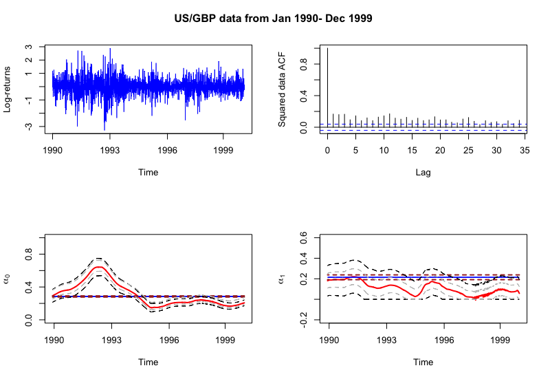
Figure 1: Analysis of USD/GBP data from Jan 1990 to Dec 1999. Top left: Log-returns. Top right: ACF plot. Bottom panel: Estimates of the parameters $\alpha_{0}(\cdot)$, $\alpha_{1}(\cdot)$, respectively (red) with 95% SCBs (dashed) and estimates of the parameters assuming constancy (blue). We also provide pointwise bands (grey) and time-constant estimate $\pm$ standard error band (brown). Optimal bandwidth was 0.26 and $\alpha_{0}(\cdot)$ is time-varying

Based on Figure 1, time-constancy for the parameter curve $\alpha_{0}(\cdot)$ is rejected at 5% level of significance. For $\alpha_{1}(\cdot)$, the estimate generally stays below the stationary fit. This can be explained by the geometry of the parameter space of the GARCH model, cf. [hillebrand_garch]. Also, one can see from the plot of actual log-returns that there are large shocks from 1990 to 1993 compared to those seen in 1993-1999. This can be explained through the high (low) values shown for the estimated curve $\alpha_{0}(\cdot)$ for the time-period 1990-1993 (1993-1999).

5.2.2 Real data application II: NASDAQ index data

In the empirical analysis of log-returns for stock market data, Palm [40] and others have found that lower order GARCH models account sufficiently for conditional heteroscedasticity. Moreover, GARCH(1,1) and in a very few cases GARCH(1,2) and GARCH(2,1) models are used and higher order GARCH models are typically not necessary. Another advantage of using GARCH(1,1) over ARCH($p$) models is that one does not need to worry about choosing a proper lag $p$ as GARCH(1,1) can be thought as an ARCH model with $p=\infty$. In this subsection, we implement a time-varying version of GARCH(1,1) and obtain the bootstrapped SCB. A tvGARCH(1,1) model has the following form:

$$Y_{i}^{2}=\sigma_{i}^{2}\zeta_{i}^{2},\quad\quad\sigma_{i}^{2}=\alpha_{0}(i/n)+\alpha_{1}(i/n)Y_{i-1}^{2}+\beta_{1}(i/n)\sigma_{i-1}^{2}.$$

As our second example, we choose to analyze the log returns of NASDAQ from January 2011 to December 2018. This is an important index in the US stock market. We collect this one and all other stock index datasets in later analysis from www.investing.com. Our cross-validated bandwidth is $b_{n}=0.405$ for this dataset of size $n=1751$. Since our simulations show excellent performance for sample sizes around $n=2000$ and the estimated parameter functions satisfy the parameter restriction $\sup_{0\leq t\leq 1}(\hat{\beta}_{1}(t)^{2}+2\hat{\alpha}_{1}(t)\hat{\beta}_{1}(t)+3\hat{\alpha}_{1}(t)^{2})<1$, it is reasonable to say our simultaneous confidence bands would also be valid here. As one can see from Figure 2, the time series shows significant lags in its ACF plot after squaring; indicating conditional heteroscedasticity.

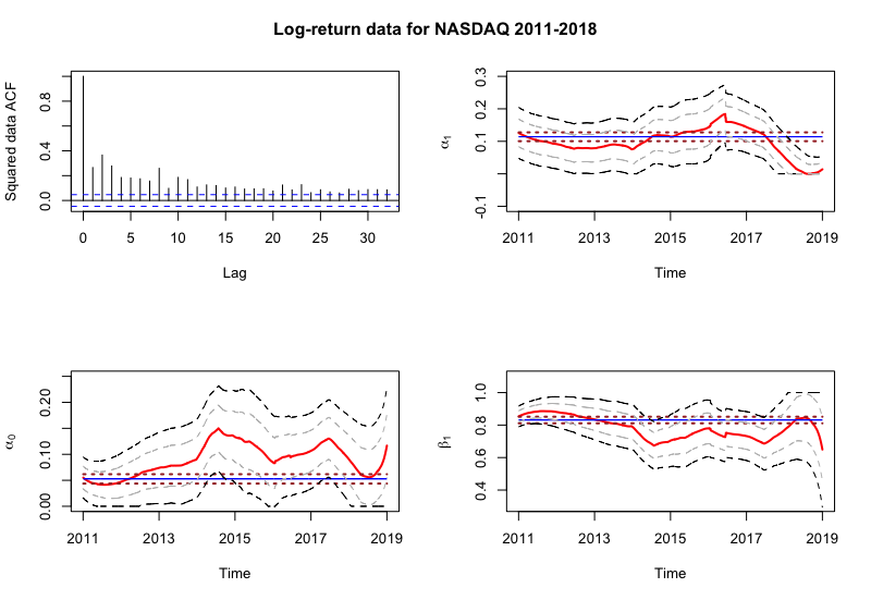
Figure 2: Analysis of Nasdaq data from Jan 2011 to Dec 2018. Top left: ACF plot. Top right, bottom left, bottom right: Estimates of the parameters $\alpha_{0}(\cdot)$, $\alpha_{1}(\cdot)$ and $\beta_{1}(\cdot)$, respectively (red) with SCBs (dashed) and estimates of the parameters assuming constancy (blue). We also provide pointwise bands (grey) and time-constant estimate $\pm$ standard error band (brown). Optimal bandwidth was 0.405. A horizontal line does not pass through the SCB of $\alpha_{1}(\cdot)$ and thus it is time-varying.

One can see that the estimates for $\alpha_{0}(\cdot)$ is mostly above the corresponding time-constant fit. As mentioned in the caption $\alpha_{1}(\cdot)$ is time-varying since the SCB does not contain a horizontal line. The fit fluctuates around the time-constant fit. For $\beta_{1}(t)$, the time-varying fit is below the corresponding time-constant fit. Overall, since $\alpha_{1}(t)$ is deemed time-varying through this analysis the time-constant hypothesis can be rejected at 5% level of significance.

5.3 Forecasting volatility

It is a legitimate question whether time-varying models in forecasting econometric time-series are more useful compared to their time-constant analogue. Note that the main goal of this paper is not to build better forecasting models. The extension to predictive intervals from confidence intervals for conditional heteroscedastic models is not very straight-forward. Moreover, it is unclear how in-fill asymptotics discussed in this paper would extend to forecasting future trends or estimate time-varying functions with time arguments $t>1$ in the future. Any asymptotic theory would need to consider the rescaling mechanism rigorously, keeping in mind the data observed up to a certain point. In this subsection we show empirically that time-varying models can indeed lead to better forecasts compared to time-constant analogues.

5.3.1 Short-range forecasts

Following [46] and [21], we show for a wide range of econometric datasets that time-varying models can provide better short range forecasts. We also allow multiple windows of forecasting and multiple start points to highlight why most of these datasets call for a time-varying fit. In the following Tables 4 and 5, we use ARCH(1) models for the forex datsets and GARCH(1,1) for the stock market indices. Our POOS (pseudo-out-of-sample) evaluation of forecasting is chalked out as follows:

Define, for a $h-$step ahead forecasting scheme, $\bar{\sigma}^{2}_{t,t+h}=\frac{1}{h}\sum_{i=t+1}^{t+h}\sum\sigma_{i|t}^{2}$ where $\sigma_{i|t}^{2}$ are the $(i-t)$ step ahead forecasts of time-constant or time-varying fit at time $t$. We compare this with the ‘realized’ volatility $\bar{X}^{2}_{t,t+h}=\frac{1}{h}\sum_{i=t+1}^{t+h}X_{i}^{2}$. We then compute the aggregated measure for a start point $s$ as following:

$$AMSE=\frac{1}{n-h-s}\sum_{s+1}^{n-h}(\bar{\sigma}^{2}_{t,t+h}-\bar{X}^{2}_{t,t+h}).$$

For the forecasting horizon $h$ values, we choose $h\in\{25,50,75,100,150,200\}$ and start points $s\in\{500,1000\}$. Our forecasting method is the same as the one implemented in the fGARCH R-package. For the time-constant fit at time $t$ we use the data from 1 to $t$ to predict the $h$-step ahead forecast. For the time-varying fit however, it is unclear what the time-varying projection will be. Following [21], we assume the last $m$ points to be stationary for a small $m$ and use that to obtain the future forecasts. Since $m$ is a tuning parameter, we choose the value that produces the minimum $AMSE$ over $m\in\{100,200,\ldots,500\}$.

Table 4: Forecasting volatility: Short range forecast comparison of time-varying and time-constant model for startpoint at 500. TV and TC stands for time-varying and time-constant models

	ahead=25		ahead=50		ahead=75		ahead=100		ahead=150		ahead=200
$Data$	TC	TV	TC	TV	TC	TV	TC	TV	TC	TV	TC	TV
USGBP	0.101	0.07	0.085	0.057	0.078	0.053	0.075	0.052	0.07	0.048	0.067	0.046
USCHF	2.968	2.775	1.702	1.528	1.269	1.115	1.048	0.099	0.803	0.601	0.646	0.524
USCAD	0.029	0.026	0.024	0.024	0.022	0.023	0.02	0.021	0.017	0.018	0.015	0.017
EURGBP	0.083	0.074	0.057	0.048	0.044	0.036	0.039	0.032	0.034	0.029	0.028	0.025
EURUSD	0.052	0.033	0.044	0.028	0.041	0.027	0.042	0.028	0.038	0.032	0.036	0.038
SP Merval	7.722	7.094	6.632	4.679	5.317	4.376	5.763	4.514	5.372	4.529	5.086	4.620
BSE	3219	3038	2916	1901	2313	2040	2259	1321	2000	1106	1897	1038
SP500 old	5.475	5.346	8.752	7.511	4.265	4.048	3.339	2.344	2.092	1.079	1.768	0.939
SP500	0.319	0.042	0.379	0.372	0.249	0.324	0.304	0.306	0.277	0.280	0.269	0.274
Dow Jones	0.037	0.0365	0.316	0.277	0.223	0.231	0.215	0.200	0.185	0.183	0.169	0.176
FTSE	0.470	0.461	0.456	0.283	0.322	0.279	0.346	0.206	0.336	0.240	0.319	0.278
NASDAQ	0.424	0.399	0.498	0.237	0.283	0.233	0.404	0.175	0.388	0.200	0.364	0.218
Smallcap	0.448	0.292	1.035	0.189	0.398	0.157	0.981	0.143	0.979	0.144	0.970	0.143
NYSE	0.318	0.245	0.470	0.144	0.277	0.148	0.418	0.107	0.413	0.121	0.404	0.136
DAX	0.903	0.800	1.142	0.559	0.639	0.552	0.992	0.501	0.961	0.580	0.920	0.697
Apple	3.736	3.535	1.853	2.100	2.069	1.816	1.380	1.787	1.305	1.818	1.280	1.749
Microsoft	2.729	3.388	1.600	1.999	1.156	1.898	0.981	1.335	0.766	1.084	0.664	0.973
AXP	2.350	2.13	2.142	1.500	1.456	1.264	1.726	1.065	1.759	0.984	1.625	0.928

Table 5: Forecasting volatility: Short range forecast comparison of time-varying and time-constant model for startpoint at 1000. TV and TC stands for time-varying and time-constant models

	ahead=25		ahead=50		ahead=75		ahead=100		ahead=150		ahead=200
$Data$	TC	TV	TC	TV	TC	TV	TC	TV	TC	TV	TC	TV
USGBP	0.068	0.019	0.064	0.017	0.062	0.015	0.061	0.014	0.059	0.013	0.058	0.014
USCHF	4.344	4.009	1.796	1.584	1.074	0.891	0.799	0.624	0.559	0.392	0.419	0.278
USCAD	0.029	0.028	0.024	0.027	0.022	0.024	0.019	0.023	0.017	0.021	0.015	0.020
EURGBP	0.019	0.012	0.017	0.011	0.016	0.010	0.015	0.009	0.015	0.010	0.014	0.011
EURUSD	0.039	0.028	0.034	0.029	0.032	0.031	0.032	0.034	0.029	0.040	0.027	0.045
SP Merval	10.39	8.714	9.432	6.12	7.666	6.029	8,522	5.883	7.908	5.857	7.052	5.739
BSE	2478	2126	2798	1437	1506	949	2288	783	2263	771	2362	945.9
SP500 OlD	8.104	7.964	12.57	11.26	6.242	5.949	4.292	3.469	2.307	1.463	1.741	1.216
SP500	0.371	0.503	0.328	0.276	0.259	0.236	0.231	0.196	0.183	0.166	0.155	0.152
DowJones	0.484	0.509	0.351	0.400	0.263	0.335	0.210	0.292	0.167	0.267	0.145	0.238
FTSE	0.644	0.639	0.514	0.378	0.409	0.394	0.358	0.270	0.347	0.353	0.314	0.419
NASDAQ	0.519	0.505	0.482	0.345	0.332	0.377	0.340	0.267	0.312	0.338	0.284	0.365
Smallcap	0.457	0.374	0.671	0.243	0.338	0.243	0.558	0.229	0.488	0.232	0.433	0.206
NYSE	0.375	0.329	0.374	0.207	0.271	0.212	0.287	0.153	0.260	0.194	0.237	0.228
DAX	1.245	1.123	1.130	0.755	0.842	0.708	0.925	0.762	0.897	0.896	0.832	1.102
Apple	2.465	2.275	1.799	1.279	1.530	1.206	1.374	0.871	1.276	1.036	1.237	1.052
Microsoft	2.868	3.668	1.720	2.295	1.214	2.147	1.057	1.596	0.851	1.335	0.770	1.232
AXP	2.837	2.668	1.749	1.462	1.395	1.347	1.151	0.825	0.982	0.681	0.834	0.581

One can see from Table 4 and 5 how for a wide range of datasets, starting points and forecasting horizons the AMSE of the time-varying forecast is considerably smaller than the one for the time-constant version. We believe, even if prediction and forecasting is more important from an economist’s perspective, this POOS analysis provides a strong motivation to choose a time-varying model over a time-constant one.

5.3.2 One-step ahead forecasting and semi-timevarying models from inference

We use the following one-step ahead $AMSE_{1}$, inspired from [45] to validate our models:

$$AMSE_{1}=\frac{1}{n}\sum_{i=1}^{n}(X_{i}^{2}-\hat{\sigma}^{2}(i/n))^{2}$$

.

Here, $X_{t}$ are the log-returns and $\hat{\sigma}^{2}(\cdot)$ refers to the fitted model using ARCH(1) for foreign exchange datasets, and GARCH(1,1) for stock market indices. In each row we exhibit the best model in bold.

Table 6: Forecasting volatility: Choosing between asymptotically 95% correct time-varying, semi-time-varying and time-constant models

Index (opt $\hat{b}_{n}$)	Time-varying	Time-constant	Time-constant coefficients	Semi-timevarying model
USGBP (0.26)	0.5701109	0.5956046	$\alpha_{1}$	0.5697231
USCHF (0.24)	45.42274	45.61378	None	NA
USCAD (0.22)	0.1604907	0.1672808	$\alpha_{1}$	0.1616965
EURGBP (0.34)	0.778459	0.789287	$\alpha_{1}$	0.7837281
EURUSD (0.23)	0.3234517	0.3399221	None	NA
SP Merval (0.36)	60.62419	62.02226	$\alpha_{1},\beta_{1}$	61.58843
SP500 old (0.29)	26.48272	26.12195	None	NA
SP500 recent (0.22)	3.54	3.527918	$\alpha_{1},\beta_{1}$	3.529355
Wilshire 5k (0.35)	1.943517	1.964926	$\alpha_{0},\alpha_{1},\beta_{1}$	1.972347
FTSE (0.45)	3.650331	3.687818	None	NA
NASDAQ (0.405)	5.4258546	5.446805	$\alpha_{1},\beta_{1}$	5.611163
Smallcap (0.35)	12.36647	12.56344	$\alpha_{1},\beta_{1}$	12.53796
NYSE (0.24)	4.830424	4.841198	$\alpha_{0},\beta_{1},\beta_{1}$	5.287622
DAX (0.44)	9.908042	9.987583	None	NA
Apple (0.27)	48.06839	46.4968	None	NA
Microsoft (0.39)	38.08752	38.33715	None	NA
AXP (0.28)	37.39755	37.90381	$\alpha_{1},\beta_{1}$	38.1988

Note that the examples exhibited here show that often the time-constant model has poor one-step ahead forecasting quality compared to their time-varying analogue. However, from Table 6, one can see that in some of these time-varying models, we have a subset of parameters not rejecting the hypothesis of time-constancy. We suspect that setting a subset of parameters to be time-constant and allowing the rest to vary over time can improve forecasting over both models. One finding of this analysis is that for some of the datasets such as USGBP, the semi-time-varying model may outperform the time-constant model in terms of forecasting. Note that it is easy to tailor and find time-constant fits that allow for even better forecasts, but those models do not have proper confidence (in terms of closeness to the true model) for the already observed data. For the numbers in the above table on the semi-time-varying column, we kept the time-varying coefficients as they are and searched for the best (in terms of $AMSE_{1}$) constant for the time-constant coefficients among the horizontal lines that fit within the bands entirely. Here we would like also to put a word of caution: Note that the semi-time-varying analysis is somewhat adhoc. In principle, one can also re-run the optimization by fitting only a proper subset as time-varying and the rest as time-constant. We have checked this with multiple of the above datasets and the AMSE were not too different from that reported above. The major takeaway from this analysis remains that our time-varying fit, albeit not meant for prediction and constructed only for building simultaneous confidence intervals, can achieve better forecasts than the corresponding time-constant fits. Additionally, our theory can also lead to new models which have only a subset of coefficients time-varying.

6 Acknowledgement

We are grateful to the editor, associate editor and two anonymous referees for their valuable comments and feedback in different rounds which has helped in significantly improving this paper. This research was partially supported by NSF/DMS 1405410.

Appendix A Technical tools and more general assumptions

A.1 The functional dependence measure

To state the structure of dependence we use throughout the appendix, we introduce a functional dependence measure on the underlying process using the idea of coupling as done in Wu [50]. Let $q>0$ and let $Z_{i}$, $i\in\mathbb{Z}$ a stationary process which admits the causal representation

$$Z_{i}=J(\zeta_{i},\zeta_{i-1},\ldots).$$ (A.1)

Suppose that $(\zeta^{*}_{i})_{i\in\mathbb{Z}}$ is an independent copy of $(\zeta_{i})_{i\in\mathbb{Z}}$. For some random variable $Z$, let $\|Z\|_{q}:=(\mathbb{E}|Z|^{q})^{1/q}$ denote the $\mathcal{L}_{q}$-norm of $Z$. For $i\geq 0$, define the functional dependence measure

$$\delta^{Z}_{q}(i)=\|Z_{i}-Z_{i}^{*}\|_{q},$$ (A.2)

where $Z_{i}^{*}=J(\mathcal{F}_{i}^{*})$ with

$$\mathcal{F}^{*}_{i}=(\zeta_{i},\zeta_{i-1},\cdots,\zeta_{1},\zeta_{0}^{*},\zeta_{-1},\zeta_{-2},\cdots)$$ (A.3)

a coupled version of $\mathcal{F}_{i}$ with $\zeta_{0}$ in $\mathcal{F}_{i}$ replaced by an independent copy $\zeta_{0}^{*}$. Note that $\delta_{q}^{Z}(i)$ measures the dependence of $Z_{i}$ on $\zeta_{0}$ in terms of the $q$th moment. The tail cumulative dependence measure $\Delta^{Z}_{q}(j)$ for $j\geq 0$ is defined as

$$\Delta^{Z}_{q}(j)=\displaystyle\sum_{i=j}^{\infty}\delta_{q}^{Z}(i).$$ (A.4)

Let $\alpha>0$. We define the adjusted dependence measure $\|\cdot\|_{q,\alpha}$ as follows (cf. [57]): For a stationary process $Z_{i}=J(\zeta_{i},\zeta_{i-1},...)$, let

$$\|Z\|_{q,\alpha}:=\sup_{m\geq 0}(m+1)^{\alpha}\Delta^{Z}_{q}(m).$$

A.2 The class $\mathcal{H}(M,\chi,\bar{C})$ for Case 1

To prove uniform convergence of $L_{n,b_{n}}^{c}$ and its derivatives w.r.t. $\theta$, we require the objective function $\ell$ introduced in Section 2.2 to be Lipschitz continuous in the direction of $\theta$ and to grow at most polynomially in the direction of $z=(y,x)$, where the degree is measured by real numbers $M\geq 1$. We will therefore ask $\ell$ and its derivatives to be in the class $\mathcal{H}(M,\chi,\bar{C})$ which is now defined.

Let $\chi=(\chi_{i})_{i=1,2,\ldots}$ be a sequence of nonnegative real numbers with $|\chi|_{1}:=\sum_{i=1}^{\infty}\chi_{i}<\infty$, and $\bar{C}>0$ be some constant. Let $|x|_{\chi,s}:=(\sum_{j=1}^{\infty}\chi_{j}|x|^{s})^{1/s}$, and put $|x|_{\chi}:=|x|_{\chi,1}$. Put $\hat{\chi}=(1,\chi)$.

A function $g:\mathbb{R}^{\mathbb{N}}\times\Theta\to\mathbb{R}$ is in $\mathcal{H}(M,\chi,\bar{C})$ if $\sup_{\theta\in\Theta}|g(0,\theta)|\leq\bar{C}$,

$$\sup_{z}\sup_{\theta\not=\theta^{\prime}}\frac{|g(z,\theta)-g(z,\theta^{\prime})|}{|\theta-\theta^{\prime}|_{1}(1+|z|_{\hat{\chi}}^{M})}\leq\bar{C}$$

and

$$\sup_{\theta}\sup_{z\not=z^{\prime}}\frac{|g(z,\theta)-g(z^{\prime},\theta)|}{|z-z^{\prime}|_{\hat{\chi}}\cdot(1+|z|_{\hat{\chi}}^{M-1}+|z^{\prime}|_{\hat{\chi}}^{M-1})}\leq\bar{C}.$$

If $g$ is vector- or matrix-valued, $g\in\mathcal{H}(M,\chi,\bar{C})$ means that every component of $g$ is in $\mathcal{H}(M,\chi,\bar{C})$.

A.3 A more general set of assumptions

We show the main theorems under a more general set of assumptions which contain more ‘high-level’ properties of the process $Y_{i}$ and the objective function $\ell$. These assumptions can therefore be seen as an ‘intermediate step’ in our proofs: We first derive these high-level properties of the processes $Y_{i}$ which hold under the more specific Assumptions 2.2 and 2.3. These high-level assumptions are given in Assumption A.1 and E.8. In Section E at the end of the supplementary material we show that Assumption 2.2 implies Assumption A.1 and Assumption 2.3 implies Assumption E.8. To keep the presentation concise, we only state Assumption A.1 here in the main part of the paper.

For each $t\in[0,1]$, let $\tilde{Y}_{i}(t)=\tilde{J}(t,\mathcal{F}_{i})$ with some measurable function $\tilde{J}$. This process serves as a stationary approximation of the observed process $Y_{i}$ (cf. the introduction in Section 3). The necessary properties are made rigorous in Assumption A.1 (for Case 1) or Assumption E.8 (for Case 2) below. Recall that $X_{i}:=(Y_{j}:-\infty<j\leq i-1)$ and $Z_{i}:=(Y_{i},X_{i})$, and $\tilde{X}_{i}(t):=(\tilde{Y}_{j}(t):-\infty<j\leq i-1)$, $\tilde{Z}_{i}(t):=(\tilde{Y}_{i}(t),\tilde{X}_{i-1}(t))$.

Assumption A.1.

Suppose that for some $r\geq 2$ and some $\gamma>1$,

1. (Smoothness in $\theta$-direction) $\ell$ is twice continuously differentiable w.r.t. $\theta$. It holds that $\ell,\nabla_{\theta}\ell,\nabla^{2}_{\theta}\ell\in\mathcal{H}(M,\chi,\bar{C})$ for some $M\geq 1$, $\bar{C}>0$ and $\chi=(\chi_{i})_{i=1,2,\ldots}$ with $\chi_{i}=O(i^{-(1+\gamma)})$.

2. (Assumptions on unknown parameter curve) $\Theta$ is compact and for all $t\in[0,1]$, $\theta(t)$ lies in the interior of $\Theta$. Each component of $\theta(\cdot)$ is in $C^{3}[0,1]$.

3. (Correct model specification) For all $t\in[0,1]$, the function $\theta\mapsto L(t,\theta):=\mathbb{E}\ell(\tilde{Z}_{0}(t),\theta)$ is uniquely minimized by $\theta(t)$.

4. The eigenvalues of the matrices $V(t)$, $I(t)$ and $\Lambda(t)$ defined in (3.1), (3.2) and (3.3) are bounded from below by some $\lambda_{0}>0$, uniformly in $t$.

5. (Stationary approximation) There exist $C_{A},C_{B},D>0$ such that for all $n\in\mathbb{N}$, $i=1,\ldots,n$, $t,t^{\prime}\in[0,1]$:

   $$\max\{\|Y_{i}\|_{rM},\ \|\tilde{Y}_{0}(t)\|_{rM}\}\leq D,$$

   $$\|Y_{i}-\tilde{Y}_{i}(i/n)\|_{rM}\leq C_{A}n^{-1},\quad\quad\|\tilde{Y}_{0}(t)-\tilde{Y}_{0}(t^{\prime})\|_{rM}\leq C_{B}|t-t^{\prime}|$$ (A.5)

6. (Weak dependence) $\sup_{t\in[0,1]}\delta_{rM}^{\tilde{Y}(t)}(k)=O(k^{-(1+\gamma)})$.

Appendix B Proofs of the theorems

In this section, we show the validity of the theorems stated in the paper under the more general Assumption A.1 or Assumption E.8, respectively. We make use of the elementary lemmas derived in Section D. Let us introduce some notation. For $\eta=(\eta_{1},\eta_{2})\in\Theta\times(\Theta^{\prime}\cdot b_{n})=:E_{n}$, define

$$L^{\circ,c}_{n,b_{n}}(t,\eta):=(nb_{n})^{-1}\sum_{i=1}^{n}K_{b_{n}}(i/n-t)\ell(Z_{i}^{c},\eta_{1}+\eta_{2}(i/n-t)b_{n}^{-1})$$

and $\hat{L}_{n,b_{n}}^{\circ}$, $L_{n,b_{n}}^{\circ}$ similarly as $L_{n,b_{n}}^{\circ,c}$ but with $Z_{i}^{c}$ replaced by $\tilde{Z}_{i}(i/n)$ or $Z_{i}$, respectively. Furthermore, put

$$\eta_{b_{n}}(t)=(\theta(t)^{\mkern-1.5mu\mathsf{T}},b_{n}\theta^{\prime}(t)^{\mkern-1.5mu\mathsf{T}})^{\mkern-1.5mu\mathsf{T}}.$$

$\eta_{b_{n}}(t)$ is estimated by

$$\hat{\eta}_{b_{n}}(t)=(\hat{\theta}_{b_{n}}(t)^{\mkern-1.5mu\mathsf{T}},b_{n}\widehat{\theta}_{b_{n}}^{\prime}(t)^{\mkern-1.5mu\mathsf{T}})^{\mkern-1.5mu\mathsf{T}}\in\mathop{\rm argmin}_{\eta\in E_{n}}L_{n,b_{n}}^{\circ,c}(t,\eta).$$

B.1 Proof of Theorem 3.2

Proof B.1 (Proof of Theorem 3.2).

By Proposition E.6, Assumption A.1 is fulfilled with some $r>2$. By Proposition E.9, Assumption E.8 is fulfilled with some $r>2$. In the following, we will only use the more general Assumptions A.1 or E.8, respectively.

By Lemma D.3(i),(iii)(a) and Lemma D.5(a) (in case Assumption A.1 holds) or Lemma D.3(i),(iii)(c) and Lemma D.5(a) (if Assumption E.8 holds) applied to $g=\ell$, we have that

$$\sup_{t\in\mathcal{T}_{n}}\sup_{\eta\in E_{n}}|L_{n,b_{n}}^{\circ,c}(t,\eta)-L^{\circ}(t,\eta)|=O_{\mathbb{P}}(\beta_{n}+(nb_{n})^{-1})+O(b_{n}),$$

where

$$L^{\circ}(t,\eta):=\int_{-1}^{1}K(x)L(t,\eta_{1}+\eta_{2}x)dx.$$

That is, $L_{n,b_{n}}^{\circ,c}(t,\eta)$ converges to $L^{\circ}(t,\eta)$ uniformly in $t,\eta$ if $b_{n}=o(1)$ and $\beta_{n}=o(1)$. By Lemma D.7, $\eta\mapsto L^{\circ}(t,\eta)$ is Lipschitz continuous in both components. Since $\theta(t)$ is the unique minimizer of $\theta\mapsto L(t,\theta)$, we have that $\eta(t)=(\theta(t)^{\mkern-1.5mu\mathsf{T}},0)^{\mkern-1.5mu\mathsf{T}}$ is the unique minimizer of $\eta\mapsto L^{\circ}(t,\eta)$. Since $\hat{\eta}_{b_{n}}(t)=(\hat{\theta}_{b_{n}}(t)^{\mkern-1.5mu\mathsf{T}},b_{n}\widehat{\theta}_{b_{n}}^{\prime}(t)^{\mkern-1.5mu\mathsf{T}})^{\mkern-1.5mu\mathsf{T}}$ is a minimizer of $L_{n,b_{n}}^{\circ,c}(t,\eta)$, standard arguments yield

$$\sup_{t\in\mathcal{T}_{n}}|\hat{\eta}_{b_{n}}(t)-\eta(t)|=o_{\mathbb{P}}(1).$$

Since $\sup_{t\in\mathcal{T}_{n}}|\eta(t)-\eta_{b_{n}}(t)|=o(1)$, we have

$$\sup_{t\in\mathcal{T}_{n}}|\hat{\eta}_{b_{n}}(t)-\eta(t)|=o_{\mathbb{P}}(1).$$ (B.1)

Thus for $n$ large enough, $\hat{\eta}_{b_{n}}(t)$ is in the interior of $E_{n}$ uniformly in $t$. By a Taylor expansion, we obtain for each $t\in\mathcal{T}_{n}$:

$$\hat{\eta}_{b_{n}}(t)-\eta_{b_{n}}(t)=-\big{[}V^{\circ}(t)+R_{n,b_{n}}(t)\big{]}^{-1}\cdot\nabla_{\eta}L_{n,b_{n}}^{\circ,c}(t,\eta_{b_{n}}(t)),$$ (B.2)

where

$$R_{n,b_{n}}(t)=\nabla_{\eta}^{2}L_{n,b_{n}}^{\circ,c}(t,\bar{\eta}(t))-V^{\circ}(t)$$

with some $\bar{\eta}(t)\in E_{n}$ satisfying $|\bar{\eta}(t)-\eta_{b_{n}}(t)|_{1}\leq|\hat{\eta}_{b_{n}}(t)-\eta_{b_{n}}(t)|_{1}$, and

$$V^{\circ}(t):=\begin{pmatrix}1&0\\ 0&\mu_{K,2}\end{pmatrix}\otimes V(t).$$ (B.3)

By Lemma D.3(i),(iii)(a) and Lemma D.5(a) (if Assumption A.1 holds) or Lemma D.3(i),(iii)(c) and Lemma D.5(b) (if Assumption E.8 holds) applied to $g=\nabla_{\theta}^{2}\ell$ and $\hat{K}(x)=K(x)$, $\hat{K}(x)=K(x)x$ or $\hat{K}(x)=K(x)x^{2}$, respectively, we have for some fixed $\iota^{\prime}>0$:

$$\sup_{t\in\mathcal{T}_{n}}\sup_{|\eta-\eta_{b_{n}}(t)|<\iota^{\prime}}|\nabla_{\eta}^{2}L_{n,b_{n}}^{\circ,c}(t,\eta)-V^{\circ}(t,\eta)|=O_{\mathbb{P}}(\beta_{n}+(nb_{n})^{-1})+O(b_{n}),$$ (B.4)

where

$$V^{\circ}(t,\eta)=\int_{-1}^{1}K(x)\begin{pmatrix}1&x\\ x&x^{2}\end{pmatrix}\otimes V(t,\eta_{1}+\eta_{2}x)dx.$$ (B.5)

For the moment, let $\tilde{h}_{i}(t)=\nabla_{\theta}\ell(\tilde{Z}_{i}(t),\theta(t))$. Note that $\mathbb{E}\tilde{h}_{0}(t)=\mathbb{E}\nabla_{\theta}\ell(\tilde{Z}_{0}(t),\theta(t))=0$ by Assumption A.1(A3), (A1) (or Assumption E.8(A3’), (A1’)).

By Lemma D.13(i) (if Assumption A.1 holds) or Lemma D.15(i) (if Assumption E.8 holds), we have $\sup_{t}\delta_{2+\varsigma}^{\tilde{h}(t)_{j}}(k)=\sup_{t}\delta_{2+\varsigma}^{\nabla_{\theta_{j}}\ell(\tilde{Z}(t),\theta(t))}(k)=O(k^{-(1+\gamma)})$ for each $j=1,\ldots,d_{\Theta}$. Using Lemma D.7 (if Assumption A.1 holds) or Lemma D.11 (if Assumption E.8 holds), we see that the conditions of Lemma B.4 are fulfilled and thus, applied to $\tilde{h}_{i}(t)$,

$$\sup_{t\in\mathcal{T}_{n}}\big{|}(nb_{n})^{-1}\sum_{i=1}^{n}K_{b_{n}}(i/n-t)\nabla_{\theta}\ell(\tilde{Z}_{i}(i/n),\theta(i/n))\big{|}=O_{\mathbb{P}}((nb_{n})^{-1/2}\log(n)).$$ (B.6)

With Lemma C.7, we obtain

$$\sup_{t\in\mathcal{T}_{n}}\big{|}\nabla_{\eta}\hat{L}_{n,b_{n}}^{\circ}(t,\eta_{b_{n}}(t))-\mathbb{E}\nabla_{\eta}\hat{L}_{n,b_{n}}^{\circ}(t,\eta_{b_{n}}(t))\big{|}=O_{\mathbb{P}}((nb_{n})^{-1/2}\log(n)+\beta_{n}b_{n}^{2}).$$

Since $\mathbb{E}\nabla_{\theta}\ell(\tilde{Z}_{0}(t),\theta(t))=0$, we obtain with Lemma C.3 (a bias expansion result) and Lemma D.3(i):

$$\sup_{t\in\mathcal{T}_{n}}|\nabla_{\eta_{j}}L_{n,b_{n}}^{\circ,c}(t,\eta_{b_{n}}(t))|=O_{\mathbb{P}}((nb_{n})^{-1/2}\log(n)+(nb_{n})^{-1}+\beta_{n}b_{n}^{2}+b_{n}^{1+j}),$$ (B.7)

where $j=1,2$. Since $\theta\mapsto V(t,\theta)=\mathbb{E}\nabla^{2}_{\theta}\ell(\tilde{Z}_{0}(t),\theta)$ is Lipschitz continuous (apply Lemma D.7 in case of Assumption A.1 or Lemma D.11 in case of Assumption E.8 to $\nabla^{2}\ell$), the same holds for $\eta\mapsto V^{\circ}(t,\eta)$. We conclude that with some constant $C>0$,

$$\sup_{t\in\mathcal{T}_{n}}|R_{n,b_{n}}(t)|\leq\sup_{t\in\mathcal{T}_{n}}\sup_{\eta\in E_{n}}|\nabla^{2}_{\eta}L_{n,b_{n}}^{\circ,c}(t,\eta)-V^{\circ}(t,\eta)|+C\sup_{t\in\mathcal{T}_{n}}|\hat{\eta}_{b_{n}}(t)-\eta_{b_{n}}(t)|.$$ (B.8)

Inserting (B.7), (B.8) and (B.1) into (B.2), we obtain

$$\sup_{t\in\mathcal{T}_{n}}|\hat{\eta}_{b_{n},j}(t)-\eta_{b_{n},j}(t)|=O_{\mathbb{P}}((nb_{n})^{-1/2}\log(n)+(nb_{n})^{-1}+\beta_{n}b_{n}^{2}+b_{n}^{1+j}),$$ (B.9)

where $j=1,2$. Inserting (B.9), (B.4) into (B.8), we get $\sup_{t\in\mathcal{T}_{n}}|R_{n,b_{n}}(t)|=O_{\mathbb{P}}(\beta_{n}+b_{n}+(nb_{n})^{-1})$. Together with

$$\big{|}V^{\circ}(t)\big{(}\hat{\eta}_{b_{n}}(t)-\eta_{b_{n}}(t)\big{)}-\nabla L_{n,b_{n}}^{\circ,c}(t,\eta_{b_{n}}(t))\big{|}$$

$$\leq \big{|}\big{[}I_{2k\times 2k}+V^{\circ}(t)^{-1}R_{n,b_{n}}(t)\big{]}^{-1}-I_{2k\times 2k}^{-1}\big{|}\cdot|\nabla_{\eta}L_{n,b_{n}}^{\circ,c}(t,\eta_{{}_{n}}(t))|$$

$$\leq \big{|}\big{[}I_{2k\times 2k}+V^{\circ}(t)^{-1}R_{n,b_{n}}(t)\big{]}^{-1}\big{|}\cdot\big{|}V^{\circ}(t)^{-1}R_{n,b_{n}}(t)\big{|}\cdot|\nabla_{\eta}L_{n,b_{n}}^{\circ,c}(t,\eta_{b_{n}}(t))|,$$

and (B.7) we obtain the assertion (3.4). The other result (3.5) follows from Lemma D.3(i), Lemma C.7 and Lemma C.3.

B.2 Proof of Theorem 3.3

In this section, we prove Theorem 3.3 by proving its assertion under the morel general Assumption A.1 or E.8, respectively. We first cite some auxiliary results: Lemma B.2 is a confidence band result for i.i.d. Gaussian vectors, Lemma B.4 extends this result to sums of dependent variables by using a Gaussian approximation result (Theorem B.3, cf. [53]). Theorem 3.3 is then proven by applying Lemma B.4 to a Bahadur representation of $\hat{\theta}_{b_{n}}$ from Theorem 3.2.

From Lemma 1 in [59], we adopt the following SCB result for Gaussian random vectors:

Lemma B.2.

Let $F_{n}(t)=\sum_{i=1}^{n}\hat{K}_{b_{n}}(t_{i}-t)V_{i}$, where $V_{i},i\in\mathbb{Z}$ are i.i.d. $N(0,I_{s\times s})$. $b_{n}\to 0$ and $nb_{n}/\log^{2}(n)\to\infty$. Let $m^{*}=1/b_{n}.$ Then

$$\lim_{n\to\infty}\mathbb{P}\Big{(}\frac{1}{\sigma_{\hat{K},0}\sqrt{nb_{n}}}\sup_{t\in\mathcal{T}_{n}}|F_{n}(t)|-B_{\hat{K}}(m^{*})\leq\frac{u}{\sqrt{2\log(m^{*})}}\Big{)}=\exp(-2\exp(-u)).$$ (B.10)

where $B_{\hat{K}}$ is defined in (3.7).

For the following results, let us assume that there exists some measurable function $\tilde{H}(\cdot,\cdot)$ such that for each $t\in[0,1]$, $\tilde{h}_{i}(t)=\tilde{H}(t,\mathcal{F}_{i})\in\mathbb{R}^{s}$ is well-defined. Put $S_{\tilde{h}}(i):=\sum_{j=1}^{i}\tilde{h}_{j}(j/n)$.

Theorem B.3 (Theorem 1 and Corollary 2 from Wu and Zhou [53]).

Assume that for each component $j=1,\ldots,s$:

1. $\sup_{t\in[0,1]}\|\tilde{h}_{0}(t)_{j}\|_{2+\varsigma}<\infty$,

2. $\sup_{t\not=t^{\prime}\in[0,1]}\|\tilde{h}_{0}(t)_{j}-\tilde{h}_{0}(t^{\prime})_{j}\|_{2}/|t-t^{\prime}|<\infty$,

3. $\sup_{t\in[0,1]}\delta_{2+\varsigma}^{\tilde{h}(t)_{j}}(k)=O(k^{-(\gamma+1)})$ with some $\gamma\geq 1$.

for some $\varsigma\leq 2$. Then on a richer probability space, there are i.i.d. $V_{1},V_{2},\ldots\sim N(0,I_{s\times s})$ and a process $S_{\tilde{h}}^{0}(i)=\sum_{j=1}^{i}\Sigma_{\tilde{h}}(j/n)V_{j}$ such that $(S_{\tilde{h}}(i))_{i=1,\ldots,n}\overset{d}{=}(S_{\tilde{h}}^{0}(i))_{i=1,\ldots,n}$ and

$$\max_{i=1,\ldots,n}|S_{\tilde{h}}(i)-S_{\tilde{h}}^{0}(i)|=O_{\mathbb{P}}(\pi_{n}).$$

where

$$\pi_{n}=n^{(2\varsigma+2\gamma+\gamma\varsigma)/(2\varsigma+8\gamma+4\gamma\varsigma)}\log(n)^{2\gamma(3+\varsigma)/(\varsigma+4\gamma+2\gamma\varsigma)}$$ (B.11)

and

$$\Sigma_{\tilde{h}}(t)=\big{(}\sum_{j\in\mathbb{Z}}\mathbb{E}[\tilde{h}_{0}(t)\tilde{h}_{j}(t)^{\mkern-1.5mu\mathsf{T}}]\big{)}^{1/2}.$$

The following lemma is an analogue of Lemma 2 in [59]. Since we use other Gaussian approximation rates from Theorem B.3, we shortly state the proof for completeness.

Lemma B.4.

Let the assumptions and notations from Theorem B.3 hold. Define

$$D_{\tilde{h}}(t):=(nb_{n})^{-1}\sum_{i=1}^{n}\hat{K}_{b_{n}}(i/n-t)\tilde{h}_{i}(i/n).$$

Assume that $\Sigma_{\tilde{h}}(t)$ is Lipschitz-continuous and that its smallest eigenvalue is bounded away from 0 uniformly on $[0,1]$. Assume that $\log(n)^{4}\big{(}b_{n}n^{(2\gamma+\varsigma\gamma-\varsigma)/(\varsigma+4\gamma+2\gamma\varsigma)}\big{)}^{-1}\to 0$ and $b_{n}\log(n)^{3/2}\to 0$. Then

$$\lim_{n\to\infty}\mathbb{P}\Big{(}\frac{\sqrt{nb_{n}}}{\sigma_{\hat{K},0}}\sup_{t\in\mathcal{T}_{n}}\Big{|}\Sigma_{\tilde{h}}^{-1}(t)D_{\tilde{h}}(t)\Big{|}-B_{\hat{K}}(m^{*})\leq\frac{u}{\sqrt{2\log(m^{*})}}\Big{)}=\exp(-2\exp(-u)),$$ (B.12)

Proof B.5 (Proof of Lemma B.4).

By Theorem B.3 and summation-by-parts, there exist i.i.d. $V_{i}\sim N(0,I_{s\times s})$ such that

$$\sup_{t\in(0,1)}|D_{\tilde{h}}(t)-\Xi(t)|=O_{\mathbb{P}}\Big{(}\frac{n^{\frac{2\varsigma+2\gamma+\gamma\varsigma}{2\varsigma+8\gamma+4\gamma\varsigma}}\log(n)^{\frac{2\gamma(3+\varsigma)}{\varsigma+4\gamma+2\gamma\varsigma}}}{nb_{n}}\Big{)}=O_{\mathbb{P}}\Big{(}\frac{\log(n)^{2}\big{(}b_{n}n^{\frac{2\gamma+\varsigma\gamma-\varsigma}{\varsigma+4\gamma+2\gamma\varsigma}}\big{)}^{-1/2}}{(nb_{n})^{1/2}\log(n)^{1/2}}\Big{)},$$ (B.13)

where $\Xi(t)=(nb_{n})^{-1}\sum_{i=1}^{n}\hat{K}_{b_{n}}(i/n-t)\Sigma_{\tilde{h}}(i/n)V_{i}$. Here, (B.13) is $o_{\mathbb{P}}((nb_{n})^{-1/2}\log(n)^{-1/2})$ due to

$$\log(n)^{4}\big{(}b_{n}n^{(2\gamma+\varsigma\gamma-\varsigma)/(\varsigma+4\gamma+2\gamma\varsigma)}\big{)}^{-1}\to 0.$$

Since $\Sigma_{\tilde{h}}(\cdot)$ is Lipschitz continuous by Assumption (b), we can use a standard chaining argument in $t$ (as it was done in Lemma C.7 for $\Pi_{n}(t)$) and the fact that $(nb_{n})^{-1}\sum_{i=1}^{n}(\Sigma_{\tilde{h}}(i/n)-\Sigma_{\tilde{h}}(t))\hat{K}_{b_{n}}(i/n-t)V_{i}\sim N(0,v_{n})$, with $|v_{n}|_{\infty}\leq C\frac{b_{n}}{n}$ for some constant $C>0$ to obtain

$$\sup_{t\in(0,1)}|\Xi(t)-(nb_{n})^{-1}\Sigma_{\tilde{h}}(t)\sum_{i=1}^{n}\hat{K}_{b_{n}}(i/n-t)V_{i}|$$ (B.14)

$$= \sup_{t\in(0,1)}\big{|}(nb_{n})^{-1}\sum_{i=1}^{n}\hat{K}_{b_{n}}(i/n-t)(\Sigma_{\tilde{h}}(i/n)-\Sigma_{\tilde{h}}(t))V_{i}\big{|}$$

$$= O_{\mathbb{P}}\Big{(}\frac{b_{n}\log(n)}{(nb_{n})^{1/2}}\Big{)}=O_{\mathbb{P}}\Big{(}\frac{b_{n}\log(n)^{3/2}}{(nb_{n})^{1/2}\log(n)^{1/2}}\Big{)},$$

which is $o_{\mathbb{P}}((nb_{n})^{-1/2}\log(n)^{-1/2})$ due to $b_{n}\log(n)^{3/2}\to 0$. So the result follows from Lemma B.2 in view of (B.13) and (B.14).

Proof B.6 (Proof of Theorem 3.3).

By Proposition E.6, Assumption 2.2 implies Assumption A.1 with arbitrarily large $\gamma>0$. By Proposition E.9, Assumption 2.3 implies Assumption E.8 with arbitrarily large $\gamma>0$. We now prove the statement under the more general Assumptions A.1 or E.8, respectively.

Choose $\gamma>0$ large enough such that $\frac{2\gamma+\varsigma\gamma-\varsigma}{\varsigma+4\gamma+2\gamma\varsigma}>\alpha_{exp}$. We therefore have

$$\log(n)^{4}\big{(}b_{n}n^{\frac{2\gamma+\varsigma\gamma-\varsigma}{\varsigma+4\gamma+2\gamma\varsigma}}\big{)}^{-1}\to 0$$ (B.15)

by assumption.

Let $\tilde{k}_{i}(t):=\nabla_{\theta}\ell(\tilde{Z}_{i}(t),\theta(t))$ and $\hat{K}(x)=K(x)$ or $\hat{K}(x)=K(x)x$, respectively. Define

$$\Omega_{C}(t):=(nb_{n})^{-1}\sum_{i=1}^{n}\hat{K}_{b_{n}}(i/n-t)A_{C}(i/n)^{\mkern-1.5mu\mathsf{T}}\tilde{k}_{i}(i/n)$$

and $D_{\tilde{k}}(t)=(nb_{n})^{-1}\sum_{i=1}^{n}\hat{K}_{b_{n}}(i/n-t)\tilde{k}_{i}(i/n)$. Similar to the discussion of $\Pi_{n}(t)$ in the proof of Lemma C.7 (note that the rates in (C.13) and (C.14) then change to $O(b_{n})$ instead of $O(b_{n}^{2})$), we can show that

$$\sup_{t\in(0,1)}|\Omega_{C}(t)-A_{C}(t)^{\mkern-1.5mu\mathsf{T}}\cdot D_{\tilde{k}}(t)|=O_{\mathbb{P}}(\beta_{n}b_{n})=O_{\mathbb{P}}\Big{(}\frac{b_{n}^{1/2}\log(n)}{(nb_{n})^{1/2}\log(n)^{1/2}}\Big{)},$$ (B.16)

which is $o_{\mathbb{P}}((nb_{n})^{-1/2}\log(n)^{-1/2})$ since $b_{n}\log(n)^{2}\to 0$.

$\tilde{h}_{i}(t):=A_{C}(t)^{\mkern-1.5mu\mathsf{T}}\tilde{k}_{i}(t)$ is a locally stationary process with long-run variance $\Sigma^{2}_{\tilde{h}}(t)=\Sigma^{2}_{C}(t)$. By Lemma B.4 (which is applicable due to (B.15)), we have that

$$\lim_{n\to\infty}\mathbb{P}\Big{(}\frac{\sqrt{nb_{n}}}{\sigma_{\hat{K},0}}\sup_{t\in\mathcal{T}_{n}}\big{|}\Sigma_{C}^{-1}(t)\Omega_{C}(t)\big{|}-B_{\hat{K}}(m^{*})\leq\frac{u}{\sqrt{2\log(m^{*})}}\Big{)}=\exp(-2\exp(-u)).$$ (B.17)

By Theorem 3.2, we have

$$\sup_{t\in\mathcal{T}_{n}}\big{|}V(t)\{\hat{\theta}_{b_{n}}(t)-\theta(t)\}-b_{n}^{2}\frac{\mu_{K,2}}{2}V(t)\theta^{\prime\prime}(t)-D_{\tilde{k}}(t)\big{|}$$ (B.18)

$$= O_{\mathbb{P}}\big{(}b_{n}^{3}+(nb_{n})^{-1}b_{n}^{-1/2}\log(n)^{3/2}+(nb_{n})^{-1/2}b_{n}\log(n)\big{)}$$

$$= O_{\mathbb{P}}\Big{(}\frac{(nb_{n}^{7}\log(n))^{1/2}+(nb_{n}^{2}\log(n)^{-4})^{-1/2}+b_{n}\log(n)^{3/2}}{(nb_{n})^{1/2}\log(n)^{1/2}}\Big{)},$$

which is $o_{\mathbb{P}}((nb_{n})^{-1/2}\log(n)^{-1/2})$ since $nb_{n}^{7}\log(n)\to 0$, $nb_{n}^{2}\log(n)^{-4}\to\infty$ and $b_{n}\log(n)^{2}\to 0$. Together with (B.16) and (B.17) (with $\hat{K}=K$), this implies (3.6).

Supplement: This material contains the remaining proofs of the results in the paper.

Appendix C Remaining proofs and intermediate lemmata for the proofs of the main theorems

In this section, we give the proofs for the Propositions 4.1 and 4.3 in Section 4. Moreover, we provide the remaining high-level lemmas for the proofs of the main results Theorem 3.2 and Theorem 3.3 of the paper in Section C.1 below.

Proof C.1 (Proof of Proposition 4.1).

(i) Lemma D.3(i),(iii), Lemma D.5 and the notation therein applied to $g=\nabla_{\theta}^{2}\ell$ imply

$$\sup_{t\in\mathcal{T}_{n}}|\hat{\mu}_{K,0,b_{n}}(t)\hat{V}_{b_{n}}(t)-\hat{\mu}_{K,0,b_{n}}(t)V(t)|$$ (C.1)

$$\leq \sup_{t\in\mathcal{T}_{n},\eta\in E_{n}}|G_{n}^{c}(t,\eta)-\hat{G}_{n}(t,\eta)|+\sup_{t\in\mathcal{T}_{n},\eta\in E_{n}}|\hat{G}_{n}(t,\eta)|$$

$$\quad\quad+\sup_{t\in\mathcal{T}_{n},\eta\in E_{n}}|\mathbb{E}\hat{B}_{n}(t,\eta)-V^{\circ}(t,\eta)|+\sup_{t\in\mathcal{T}_{n}}|V^{\circ}(t,\hat{\eta}_{b_{n}})-\hat{\mu}_{K,0,b_{n}}(t)V(t)|$$

$$= O_{\mathbb{P}}((nb_{n})^{-1})+o_{\mathbb{P}}(\beta_{n})+O(b_{n})+\sup_{t\in\mathcal{T}_{n}}|V^{\circ}(t,\hat{\eta}_{b_{n}})-\hat{\mu}_{K,0,b_{n}}(t)V(t)|.$$

We obtain similar as in the proof of Theorem 3.2((B.9) therein) that

$$\sup_{t\in\mathcal{T}_{n}}|\hat{\eta}_{b_{n}}(t)-\eta_{b_{n}}(t)|=O_{\mathbb{P}}((nb_{n})^{-1/2}\log(n)+(nb_{n})^{-1}+\beta_{n}b_{n}^{2}+b_{n}^{2}).$$

Since $\eta\mapsto V^{\circ}(t,\eta)$ is Lipschitz continuous by Lemma D.7, the result follows from (C.1) and $b_{n}\log(n)\to 0$.

(ii) follows similarly due to $\nabla_{\theta}\ell\cdot\nabla_{\theta}\ell^{\mkern-1.5mu\mathsf{T}}\in\mathcal{H}(2M,\chi,\bar{\bar{C}})$ with some $\bar{\bar{C}}>0$.

Proof C.2 (Proof of Proposition 4.3).

We proceed similar as in the proof of Theorem 3.2. Now we use the explicit result of Lemma D.5(a) applied to $g=\ell$ (both for Assumption A.1 and E.8), we obtain

$$\sup_{t\in(0,1)}\sup_{\eta\in E_{n}}|L_{n,b_{n}}^{\circ}(t,\eta)-\tilde{L}_{b_{n}}^{\circ}(t,\eta)|=O_{\mathbb{P}}(\beta_{n}+(nb_{n})^{-1})+O(b_{n}),$$

where $\tilde{L}_{b_{n}}^{\circ}(t,\eta)=\int_{-t/b_{n}}^{(1-t)/b_{n}}K(x)L(t,\eta_{1}+\eta_{2}x)dx$. By optimality of $\hat{\eta}_{b_{n}}(t)$,

$$0 \leq L_{n,b_{n}}^{\circ}(t,\theta(t))-L_{n,b_{n}}^{\circ}(t,\hat{\eta}_{b_{n}}(t))$$

$$\leq \tilde{L}_{b_{n}}^{\circ}(t,\theta(t))-\tilde{L}_{b_{n}}^{\circ}(t,\hat{\eta}_{b_{n}}(t))+2\sup_{\eta\in E_{n}}|L_{n,b_{n}}^{\circ}(t,\eta)-\tilde{L}_{b_{n}}^{\circ}(t,\eta)|.$$

This implies

$$\min\Big{\{}\int_{-1}^{0}K(x)\big{\{}L(t,\hat{\theta}_{b_{n}}(t)+b_{n}\widehat{\theta}_{b_{n}}^{\prime}(t)x)-L(t,\theta(t))\big{\}}dx,$$

$$\quad\quad\int_{0}^{1}K(x)\big{\{}L(t,\hat{\theta}_{b_{n}}(t)+b_{n}\widehat{\theta}_{b_{n}}^{\prime}(t)x)-L(t,\theta(t))\big{\}}dx\Big{\}}\leq 2\sup_{\eta\in E_{n}}|L_{n,b_{n}}^{\circ}(t,\eta)-\tilde{L}_{b_{n}}^{\circ}(t,\eta)|.$$ (C.2)

Assume that for some $\iota>0$, $\limsup_{n\to\infty}\sup_{t\in(0,1)}|\hat{\eta}_{b_{n}}(t)-(\theta(t)^{\mkern-1.5mu\mathsf{T}},0)^{\mkern-1.5mu\mathsf{T}}|\geq\iota$. Then there exists $t\in(0,1)$ such that either (c1)

$$|\hat{\theta}_{b_{n}}(t)-\theta(t)|\geq\frac{1}{2}|b_{n}\widehat{\theta}_{b_{n}}^{\prime}(t)|$$

and thus $|\hat{\theta}_{b_{n}}(t)-\theta(t)|>\iota/3$, or (c2)

$$|\hat{\theta}_{b_{n}}(t)-\theta(t)|<\frac{1}{2}|b_{n}\widehat{\theta}_{b_{n}}^{\prime}(t)|,$$

and thus $|b_{n}\widehat{\theta}_{b_{n}}^{\prime}(t)|>2\iota/3$.
In case (c1), we have $|\hat{\theta}_{b_{n}}(t)+b_{n}\widehat{\theta}_{b_{n}}^{\prime}(t)x-\theta(t)|\geq|\hat{\theta}_{b_{n}}(t)-\theta(t)|-|x||b_{n}\widehat{\theta}_{b_{n}}^{\prime}(t)|\geq\frac{\iota}{6}$ for $x\in[0,\frac{1}{4}]$, thus with some $c_{0}>0$,

$$\int_{0}^{1}K(x)\big{\{}L(t,\hat{\theta}_{b_{n}}(t)+b_{n}\widehat{\theta}_{b_{n}}^{\prime}(t)x)-L(t,\theta(t))\big{\}}dx\geq\int_{0}^{1/4}K(x)\big{\{}L(t,\hat{\theta}_{b_{n}}(t)+b_{n}\widehat{\theta}_{b_{n}}^{\prime}(t)x)-L(t,\theta(t))\big{\}}dx\geq c_{0}$$

since $\theta\mapsto L(t,\theta)$ is continuous and attains its unique minimum at $\theta=\theta(t)$.
In case (c2), we have $|\hat{\theta}_{b_{n}}(t)+b_{n}\widehat{\theta}_{b_{n}}^{\prime}(t)x-\theta(t)|\geq|x||b_{n}\widehat{\theta}_{b_{n}}^{\prime}(t)|-|\hat{\theta}_{b_{n}}(t)-\theta(t)|\geq\frac{\iota}{6}$ for $x\in[\frac{3}{4},1]$, thus with some $c_{0}>0$,

$$\int_{0}^{1}K(x)\big{\{}L(t,\hat{\theta}_{b_{n}}(t)+b_{n}\widehat{\theta}_{b_{n}}^{\prime}(t)x)-L(t,\theta(t))\big{\}}dx\geq\int_{3/4}^{1}K(x)\big{\{}L(t,\hat{\theta}_{b_{n}}(t)+b_{n}\widehat{\theta}_{b_{n}}^{\prime}(t)x)-L(t,\theta(t))\big{\}}dx\geq c_{0}.$$

In both cases, (C.2) becomes a contradiction. Therefore,

$$\sup_{t\in(0,1)}|\hat{\eta}_{b_{n}}(t)-\eta_{b_{n}}(t)|=o_{\mathbb{P}}(1).$$

Using summation-by-parts and Gaussian approximation similar to that presented in Theorem B.3 for the process $\nabla_{\theta}\ell(\tilde{Z}_{i}(i/n),\theta(i/n))$, there exists i.i.d. $V_{1},V_{2},\ldots\sim N(0,I_{s\times s})$ on a richer probability space such that, for $\pi_{n}$ as in (B.11)

$$\sup_{t\in(0,1)}\big{|}(nb_{n})^{-1}\sum_{i=1}^{n}K_{b_{n}}(i/n-t)(\nabla_{\theta}\ell(\tilde{Z}_{i}(i/n),\theta(i/n))-V_{i})\big{\}}|=O_{\mathbb{P}}((nb_{n})^{-1}\pi_{n})=O_{\mathbb{P}}((nb_{n})^{-1/2}\log(n)).$$ (C.3)

Thus one can replace $\sup_{t\in\mathcal{T}_{n}}$ by $\sup_{t\in(0,1)}$ in (B.6). A careful examination of the rest of the proof of Theorem 3.2 (with Lemma C.3(C.7) replaced by Lemma C.3(C.8)) now yields the result

$$\sup_{t\in(0,1)}|\tilde{V}_{b_{n}}^{\circ}(t)\cdot(\hat{\eta}_{b_{n}}(t)-\eta_{b_{n}}(t))-\nabla_{\eta}L_{n,b_{n}}^{\circ,c}(t,\eta_{b_{n}}(t))\big{|}=O_{\mathbb{P}}(\tau_{n}^{(1)}),$$ (C.4)

where (we shortly write $\hat{\mu}_{K,j}(t)=\hat{\mu}_{K,j,b_{n}}(t)$)

$$\tilde{V}_{b_{n}}^{\circ}(t)=\begin{pmatrix}\hat{\mu}_{K,0}(t)&\hat{\mu}_{K,1}(t)\\ \hat{\mu}_{K,1}(t)&\hat{\mu}_{K,2}(t)\end{pmatrix}\otimes V(t).$$

By Lemma D.3(i), Lemma C.3 and Lemma C.7, we obtain furthermore with $U_{i,n}(t)=(K_{b_{n}}(i/n-t),K_{b_{n}}(i/n-t)\cdot(i/n-t)b_{n}^{-1})^{\mkern-1.5mu\mathsf{T}}$:

$$\sup_{t\in(0,1)}\big{|}\nabla_{\eta}L_{n,b_{n}}^{\circ,c}(t,\eta_{b_{n}}(t))-b_{n}^{2}\begin{pmatrix}\hat{\mu}_{K,2}(t)\\ \hat{\mu}_{K,3}(t)\end{pmatrix}\otimes[V(t)\theta^{\prime\prime}(t)]$$

$$\quad\quad\quad\quad-(nb_{n})^{-1}\sum_{i=1}^{n}U_{i,n}(t)\otimes\nabla_{\theta}\ell(\tilde{Z}_{i}(i/n),\theta(i/n))\big{|}=O_{\mathbb{P}}(\beta_{n}b_{n}^{2}+b_{n}^{3}+(nb_{n})^{-1}).$$ (C.5)

Recalling the proof of Lemma B.4, (B.13) and (B.14) and the proof of Theorem 3.3, (B.16) we see that there exist i.i.d. $V_{i}\sim N(0,I_{s\times s})$ such that both for $\hat{K}=K$ and $\hat{K}(x)=K(x)\cdot x$,

$$\sup_{t\in(0,1)}\big{|}A_{C}(t)^{\mkern-1.5mu\mathsf{T}}(nb_{n})^{-1}\sum_{i=1}^{n}\hat{K}_{b_{n}}(i/n-t)\nabla_{\theta}\ell(\tilde{Z}_{i}(i/n),\theta(i/n))$$ (C.6)

$$\quad\quad\quad\quad-\Sigma_{C}(t)(nb_{n})^{-1}\sum_{i=1}^{n}\hat{K}_{b_{n}}(i/n-t)V_{i}\big{|}$$

$$= O_{\mathbb{P}}\Big{(}\frac{\log(n)^{2}\big{(}b_{n}n^{\frac{2\gamma+\varsigma\gamma-\varsigma}{\varsigma+4\gamma+2\gamma\varsigma}}\big{)}^{-1/2}}{(nb_{n})^{1/2}\log(n)^{1/2}}+\frac{b_{n}\log(n)^{3/2}}{(nb_{n})^{1/2}\log(n)^{1/2}}+\frac{b_{n}^{1/2}\log(n)}{(nb_{n})^{1/2}\log(n)^{1/2}}\Big{)}$$

$$\quad\quad\quad\quad=:O_{\mathbb{P}}(w_{n}).$$

With (C.4) and

$$\tilde{V}_{b_{n}}^{\circ}(t)^{-1} = \begin{pmatrix}\hat{\mu}_{K,0}(t)&\hat{\mu}_{K,1}(t)\\ \hat{\mu}_{K,1}(t)&\hat{\mu}_{K,2}(t)\end{pmatrix}^{-1}\otimes V(t)^{-1}$$

$$= \frac{1}{\hat{\mu}_{K,2}(t)N_{b_{n}}^{(0)}(t)}\begin{pmatrix}\hat{\mu}_{K,2}(t)V(t)^{-1}&-\hat{\mu}_{K,1}(t)V(t)^{-1}\\ -\hat{\mu}_{K,1}(t)V(t)^{-1}&\hat{\mu}_{K,0}(t)V(t)^{-1}\end{pmatrix},$$

we obtain:

$$\sup_{t\in(0,1)}\Big{|}N_{b_{n}}^{(0)}(t)\cdot\{\hat{\theta}_{b_{n},C}(t)-\theta_{C}(t)\}$$

$$\quad\quad\quad\quad-\Big{[}A_{C}(t)^{\mkern-1.5mu\mathsf{T}}\nabla_{\eta_{1}}L_{n,b_{n}}^{\circ,c}(t,\eta_{b_{n}}(t))-\frac{\hat{\mu}_{K,1}(t)}{\hat{\mu}_{K,2}(t)}A_{C}(t)^{\mkern-1.5mu\mathsf{T}}\nabla_{\eta_{2}}L_{n,b_{n}}^{\circ,c}(t,\eta_{b_{n}}(t))\Big{]}\Big{|}=O_{\mathbb{P}}(\tau_{n}^{(1)}).$$

With (C.5) and (C.6), we have

$$\sup_{t\in(0,1)}\Big{|}N^{(0)}_{b_{n}}(t)\cdot\{\hat{\theta}_{b_{n},C}(t)-\theta_{C}(t)\}$$

$$\quad\quad\quad\quad\quad+b_{n}^{2}N^{(1)}_{b_{n}}(t)\theta_{C}^{\prime\prime}(t)-\Sigma_{C}(t)\big{\{}Q_{b_{n}}^{(0)}(t)-\frac{\hat{\mu}_{K,1}(t)}{\hat{\mu}_{K,2}(t)}Q_{b_{n}}^{(1)}(t)\big{\}}\Big{|}$$

$$= O_{\mathbb{P}}(\tau_{n}^{(1)}+(\beta_{n}b_{n}^{2}+b_{n}^{3}+(nb_{n})^{-1})+w_{n}),$$

which finishes the proof.

C.1 Intermediate Lemmas for $\hat{L}_{n,b_{n}}^{\circ}$

In this section, we show some lemmas for $\hat{L}_{n,b_{n}}^{\circ}$ which are needed to prove the main results. To do so, we make use of the elementary lemmas derived in Section D. Lemma C.3 derives a bias expansion of $\nabla_{\eta}\hat{L}_{n,b_{n}}^{\circ}(t,\eta_{b_{n}}(t))$, Lemma C.7 shows an approximation of $\nabla_{\eta}\hat{L}_{n,b_{n}}^{\circ}(t,\eta_{b_{n}}(t))$ by a localized sum of $\nabla_{\theta}\ell(\tilde{Z}_{i}(i/n),\theta(i/n))$, that is, the lemma justifies the replacement of the locally stationary process $Z_{i}$ in $\nabla_{\eta}\hat{L}_{n,b_{n}}^{\circ}(t,\eta_{b_{n}}(t))$ by $\tilde{Z}_{i}(i/n)$ with a certain convergence rate. Lemma C.5 discusses Lipschitz properties of a quantity $\Pi_{n}$ which occurs in the proof of Lemma C.7.

Lemma C.3.

Let $\eta_{b_{n}}(t)=(\theta(t)^{\mkern-1.5mu\mathsf{T}},b_{n}\theta^{\prime}(t)^{\mkern-1.5mu\mathsf{T}})^{\mkern-1.5mu\mathsf{T}}$. Let Assumption A.1 hold with $r=1$ or let Assumption E.8 hold with $r=2+\varsigma$, $\varsigma>0$. Then uniformly in $t\in\mathcal{T}_{n}$,

$$\mathbb{E}\nabla_{\eta_{1}}\hat{L}_{n,b_{n}}^{\circ}(t,\eta_{b_{n}}(t))=b_{n}^{2}\frac{\mu_{K,2}}{2}V(t)\theta^{\prime\prime}(t)+O(b_{n}^{3}+(nb_{n})^{-1}).$$ (C.7)

Furthermore, it holds uniformly in $t\in(0,1)$ that

$$\mathbb{E}\nabla_{\eta}\hat{L}_{n,b_{n}}^{\circ}(t,\eta_{b_{n}}(t))=\frac{b_{n}^{2}}{2}\int_{-t/b_{n}}^{(1-t)/b_{n}}K(x)\begin{pmatrix}x^{2}\\ x^{3}\end{pmatrix}dx\otimes[V(t)\theta^{\prime\prime}(t)]+O(b_{n}^{3}+(nb_{n})^{-1}).$$ (C.8)

Proof C.4 (Proof of Lemma C.3).

Let $U_{i,n}(t)=(K_{b_{n}}(i/n-t),K_{b_{n}}(i/n-t)(i/n-t)b_{n}^{-1})^{\mkern-1.5mu\mathsf{T}}$. By a Taylor expansion of $\theta(i/n)$ around $t$, we have

$$\theta(i/n)=\theta(t)+\theta^{\prime}(t)(i/n-t)+r_{n}(t),$$

where $r_{n}(t)=\theta^{\prime\prime}(t)\frac{(i/n-t)^{2}}{2}+\theta^{\prime\prime\prime}(\tilde{t})\frac{(i/n-t)^{3}}{6}$ and $\tilde{t}$ is between $t$ and $i/n$. We conclude that

$$\nabla_{\eta}\hat{L}_{n,b_{n}}^{\circ}(t,\eta_{b_{n}}(t))-(nb_{n})^{-1}\sum_{i=1}^{n}U_{i,n}(t)\otimes\nabla_{\theta}\ell(\tilde{Z}_{i}(i/n),\theta(i/n))$$ (C.9)

$$= (nb_{n})^{-1}\sum_{i=1}^{n}U_{i,n}(t)\otimes\big{\{}\int_{0}^{1}\nabla_{\theta}^{2}\ell(\tilde{Z}_{i}(i/n),\theta(i/n)+sr_{n}(t))ds\cdot r_{n}(t)\big{\}}.$$

Using $\nabla_{\theta}^{2}\ell\in\mathcal{H}(M,\chi,\bar{C})$ (if Assumption A.1 holds) or $\nabla_{\theta}^{2}\ell\in\mathcal{H}(M(1+s),\chi,\bar{C})$ with $s>0$ small enough (if Assumption E.8 holds), we obtain with Lemma D.7 for $|i/n-t|\leq b_{n}$:

$$\|\nabla_{\theta}^{2}\ell(\tilde{Z}_{i}(i/n),\theta(i/n)+sr_{n}(t))-\nabla_{\theta}^{2}\ell(\tilde{Z}_{i}(t),\theta(t))\|_{1}=O(b_{n}+n^{-1}).$$ (C.10)

Using (C.9), $\mathbb{E}\nabla_{\theta}\ell(\tilde{Z}_{i}(i/n),\theta(i/n))=0$ (which follows from Assumption A.1(A1),(A3) or Assumption E.8(A1’), (A3’)) and (C.10), we obtain

$$\mathbb{E}\nabla_{\eta}\hat{L}_{n,b_{n}}^{\circ}(t,\eta_{b_{n}}(t))$$ (C.11)

$$= (nb_{n})^{-1}\sum_{i=1}^{n}U_{i,n}(t)\otimes\big{\{}\mathbb{E}\nabla_{\theta}^{2}\ell(\tilde{Z}_{i}(t),\theta(t))\cdot\theta^{\prime\prime}(t)\frac{(i/n-t)^{2}}{2}\big{\}}+O(b_{n}^{3}+n^{-1})$$

$$= \frac{b_{n}^{2}}{2}\int_{-t/b_{n}}^{(1-t)/b_{n}}K(x)\begin{pmatrix}x^{2}\\ x^{3}\end{pmatrix}dx\otimes[V(t)\theta^{\prime\prime}(t)]+O(b_{n}^{3}+n^{-1}+(nb_{n})^{-1}),$$

which shows (C.8). Equation (C.7) follows since $t\in\mathcal{T}_{n}$ and symmetry of $K$ imply

$$\int_{-t/b_{n}}^{(1-t)/b_{n}}K(x)\begin{pmatrix}x^{2}\\ x^{3}\end{pmatrix}dx=\int_{0}^{1}K(x)\begin{pmatrix}x^{2}\\ x^{3}\end{pmatrix}dx=\begin{pmatrix}\mu_{K,2}\\ 0\end{pmatrix}.$$

Lemma C.5 (Lipschitz properties of $\Pi_{n}$).

Let $s\geq 0$. Suppose that Assumption A.1 holds with $r\geq 1$ or Assumption E.8 holds with $r>1$.

Define

$$\Pi_{n}(t):=(nb_{n})^{-1}\sum_{i=1}^{n}(M_{i}^{(2)}(t,i/n)-\mathbb{E}M_{i}^{(2)}(t,i/n)),$$

where

$$M_{i}^{(2)}(t,u)=\hat{K}_{b_{n}}(u-t)\cdot\int_{0}^{1}M_{i}(t,u)ds\cdot d_{u}(t),$$

$M_{i}(u,t)=\nabla_{\theta}^{2}\ell(\tilde{Z}_{i}(u),\theta(t)+sd_{u}(t))$ and $d_{u}(t)=\theta(u)-\theta(t)-(u-t)\theta^{\prime}(t)$. Then there exist come constants $\tilde{C},\iota^{\prime}>0$ such that

$$\Big{\|}\sup_{t\not=t^{\prime},|t-t^{\prime}|<\iota^{\prime}}\frac{|\Pi_{n}(t)-\Pi_{n}(t^{\prime})|}{|t-t^{\prime}|_{1}}\Big{\|}_{1}\leq\tilde{C}.$$

Proof C.6 (Proof of Lemma C.5).

We have

$$|M_{i}^{(2)}(t,u)-M_{i}^{(2)}(t^{\prime},u)|$$

$$\leq |\hat{K}_{b_{n}}(u-t)-\hat{K}_{b_{n}}(u-t^{\prime})|\cdot|M_{i}(t,u)|\cdot|d_{u}(t)|$$

$$\quad\quad+|\hat{K}_{b_{n}}(u-t^{\prime})|\cdot|M_{i}(t,u)-M_{i}(t^{\prime},u)|\cdot|d_{u}(t)|$$

$$\quad\quad+|\hat{K}_{b_{n}}(u-t^{\prime})|\cdot|M_{i}(t^{\prime},u)|\cdot|d_{u}(t)-d_{u}(t^{\prime})|.$$

If Assumption A.1 holds, we have $g=\nabla_{\theta}^{2}\ell\in\mathcal{H}(M,\chi,\bar{C})$. Elementary calculations show that

$$|M_{i}(t,u)| \leq \sup_{\theta\in\Theta}|g(\tilde{Z}_{i}(u),\theta)|,$$

$$|M_{i}(t,u)-M_{i}(t^{\prime},u)| \leq \sup_{\theta\in\Theta}\frac{|g(\tilde{Z}_{i}(u),\theta)-g(\tilde{Z}_{i}(u),\theta^{\prime})|}{|\theta-\theta^{\prime}|_{1}}\cdot\{|\theta(t)-\theta(t^{\prime})|_{1}+|d_{u}(t)-d_{u}(t^{\prime})|_{1}\},$$

As long as $|t-u|<1$ and $|t-t^{\prime}|$ is small enough, we obtain $|t^{\prime}-u|\leq 1$. So in the case that either $|t-u|<1$ or $|t^{\prime}-u|<1$, Lipschitz continuity of $\theta(\cdot),\theta^{\prime}(\cdot)$ implies that there exists some constant $\tilde{C}>0$ such that $|d_{u}(t)-d_{u}(t^{\prime})|_{1}\leq\tilde{C}|t-t^{\prime}|,|\theta(t)-\theta(t^{\prime})|_{1}\leq\tilde{C}|t-t^{\prime}|$, $|d_{u}(t)|_{1}\leq\tilde{C}$.

This implies

$$|M_{i}^{(2)}(t,u)-M_{i}^{(2)}(t^{\prime},u)| \leq \tilde{C}b_{n}^{-1}L_{\hat{K}}\sup_{\theta\in\Theta}|g(\tilde{Z}_{i}(u),\theta)|\cdot|t-t^{\prime}|$$ (C.12)

$$\quad+2|\hat{K}|_{\infty}\tilde{C}^{2}\cdot\sup_{\theta\in\Theta}\frac{|g(\tilde{Z}_{i}(u),\theta)-g(\tilde{Z}_{i}(u),\theta^{\prime})|}{|\theta-\theta^{\prime}|_{1}}|t-t^{\prime}|$$

$$\quad+|\hat{K}|_{\infty}\tilde{C}\cdot\sup_{\theta\in\Theta}|g(\tilde{Z}_{i}(u),\theta)|\cdot|t-t^{\prime}|.$$

With Lemma D.7(i) we obtain the result.

Suppose now that Assumption E.8 holds. As long as $|t-t^{\prime}|$ is small enough and $n$ is large enough, $|u-t|\leq b_{n}$ (or $|u-t^{\prime}|\leq b_{n}$) and the twice differentiability of $\theta(\cdot)$ imply that $\sup_{\nu\in[0,1]}|\theta(u)-(\theta(t)+\nu d_{u}(t))|_{1}<\iota$, $\sup_{\nu\in[0,1]}|\theta(u)-(\theta(t^{\prime})+\nu d_{u}(t^{\prime}))|_{1}<\iota$. Put $\tilde{\ell}_{\tilde{\theta}}(y,x,\theta)=g(F(x,\tilde{\theta},y),x,\theta)$ and $\tilde{g}=\nabla_{\theta}^{2}\tilde{\ell}$. By Assumption E.8, $\tilde{g}\in\mathcal{H}_{\iota}^{mult}(M(1+s),\chi^{(s)},\bar{C}^{(s)})$ for all $s>0$ small enough. Then

$$|M_{i}(t,u)| \leq \sup_{|\theta-\theta(u)|_{1}<\iota}|\tilde{g}_{\theta(u)}(\zeta_{i},\tilde{X}_{i}(u),\theta)|,$$

$$|M_{i}(t,u)-M_{i}(t^{\prime},u)| \leq \bar{C}\cdot\sup_{\theta\not=\theta^{\prime},|\theta-\theta(u)|_{1}<\iota,|\theta^{\prime}-\theta(u)|_{1}<\iota}\frac{|\tilde{g}_{\theta(u)}(\zeta_{i},\tilde{X}_{i}(u),\theta)-\tilde{g}_{\theta(u)}(\zeta_{i},\tilde{X}_{i}(u),\theta^{\prime})|}{|\theta-\theta^{\prime}|_{1}}$$

$$\quad\quad\times\{|\theta(t)-\theta(t^{\prime})|_{1}+|d_{u}(t)-d_{u}(t^{\prime})|_{1},$$

giving appropriate results for (C.12) and thus the assertion with Lemma D.11.

Lemma C.7.

Let $U_{i,n}(t):=K_{b_{n}}(i/n-t)\cdot(1,(i/n-t)b_{n}^{-1})^{\mkern-1.5mu\mathsf{T}}$. Let Assumption A.1 or E.8 hold with some $r=2+\varsigma$, $\varsigma>0$. Then it holds that

$$\sup_{t\in(0,1)}\big{|}\nabla_{\eta}\hat{L}_{n,b_{n}}^{\circ}(t,\eta_{b_{n}}(t))-\mathbb{E}\nabla_{\eta}\hat{L}_{n,b_{n}}^{\circ}(t,\eta_{b_{n}}(t))$$

$$\quad\quad\quad\quad\quad-(nb_{n})^{-1}\sum_{i=1}^{n}U_{i,n}(t)\otimes\nabla_{\theta}\ell(\tilde{Z}_{i}(i/n),\theta(i/n))\big{|}=O_{\mathbb{P}}(\beta_{n}b_{n}^{2}).$$

Proof C.8.

Note that $\mathbb{E}\nabla_{\theta}\ell(\tilde{Z}_{i}(i/n),\theta(i/n))=0$ by Assumption A.1(A1),(A3) or Assumption E.8(A1’),(A3’). Put

$$\Pi_{n}(t)$$

$$:= (nb_{n})^{-1}\sum_{i=1}^{n}U_{i,n}(t)\otimes\big{\{}[\nabla_{\theta}\ell(\tilde{Z}_{i}(i/n),\theta(t)+(i/n-t)\theta^{\prime}(t))-\nabla_{\theta}\ell(\tilde{Z}_{i}(i/n),\theta(i/n))]$$

$$\quad\quad\quad\quad\quad\quad\quad\quad-\mathbb{E}[\nabla_{\theta}\ell(\tilde{Z}_{i}(i/n),\theta(t)+(i/n-t)\theta^{\prime}(t))-\nabla_{\theta}\ell(\tilde{Z}_{i}(i/n),\theta(i/n))]\}.$$

We have to prove that $\sup_{t\in\mathcal{T}_{n}}\big{|}\Pi_{n}(t)\big{|}=O_{\mathbb{P}}(\delta_{n}b_{n}^{2}$). Define $M_{i}(t,u):=\int_{0}^{1}\nabla_{\theta}^{2}\ell(\tilde{Z}_{i}(u),\theta(t)+s(\theta(u)-\theta(t)-(u-t)\theta^{\prime}(t)))ds$ and $M_{i}^{(2)}(t,u)=U_{i,n}(t)\otimes\big{\{}M_{i}(t,u)\{\theta(u)-\theta(t)-(u-t)\theta^{\prime}(t)\}\big{\}}$. By a Taylor expansion of $\nabla_{\theta}\ell$ w.r.t. $\theta$, we have

$$\Pi_{n}(t)=(nb_{n})^{-1}\sum_{i=1}^{n}(M_{i}^{(2)}(t,i/n)-\mathbb{E}M_{i}^{(2)}(t,i/n)).$$

We now apply a similar technique as in the proof of Lemma D.3(iii), namely we use a chaining argument similar to (D.5) to prove

$$\mathbb{P}\big{(}\sup_{t\in(0,1)}|\Pi_{n}(t)|>Q\beta_{n}b_{n}^{2}\big{)}\to 0,$$

for some $Q>0$ large enough. Define the discretization $\mathcal{T}_{n,r}:=\{l/r:l=1,\ldots,r\}$ with $r=n^{5}$. By Lemma C.5, we have with Markov’s inequality for $Q>0$:

$$\mathbb{P}\big{(}\sup_{|t-t^{\prime}|\leq r^{-1}}|\Pi_{n}(t)-\Pi_{n}(t^{\prime})|>Q\beta_{n}b_{n}^{2}/2\big{)}=O\big{(}\frac{b_{n}^{-2}r^{-1}}{\beta_{n}b_{n}^{2}}\big{)},$$

which converges to 0. Choose $\alpha=1/2$. By Lemma D.13(iii) or Lemma D.15(iii) applied with $q=2+s$ ($s$ small enough), we obtain that $\sup_{u}\Delta_{2+s}^{\sup_{t}|M^{(2)}(t,u)|}(k)=O(k^{-(1+\gamma)})$. Thus

$$\tilde{W}_{2+s,\alpha} := \sup_{u\in[0,1]}\sup_{t\in[0,1]}\|\sup_{t,\eta}|M_{i}^{(2)}(t,u)|\|_{2+\varsigma,\alpha}=\sup_{m\geq 0}(m+1)^{\alpha}\Delta_{2+s}^{\sup_{t}|M^{(2)}(t,u)|}(m)$$ (C.13)

$$= O(b_{n}^{2})$$

(the constant being independent of $n$) and

$$\tilde{W}_{2,\alpha} := \sup_{t,u}\|M_{i}^{(2)}(t,u)\|_{2,\alpha}=\sup_{m\geq 0}(m+1)^{\alpha}\sup_{u\in[0,1]}\sup_{t}\Delta_{2}^{M^{(2)}(t,u)}(m)$$ (C.14)

$$= O(b_{n}^{2})$$

(the constant being independent of $n$). We now apply Theorem 6.2 of [57] (the proof therein also works for the uniform functional dependence measure) with $q=2+s$, $\alpha=1/2$ to $(M_{i}^{(2)}(t,i/n))_{t\in\mathcal{T}_{n,r}}$, where $l=1\vee\#(\mathcal{T}_{n,r})\leq 5\log(n)$. For $Q$ large enough, we obtain with some constant $C_{\alpha,s}>0$:

$$\mathbb{P}\big{(}\sup_{t^{\prime}\in\mathcal{T}_{n,r}}|\Pi_{n}(t^{\prime})|\geq Q\beta_{n}b_{n}^{2}/2\big{)}$$

$$\leq \frac{C_{\alpha,s}n\cdot l^{1+s/2}\tilde{W}_{2+s,\alpha}^{2+s}}{(Q/2)^{2+s}(\beta_{n}b_{n}^{2}(nb_{n}))^{2+s}}+C_{\alpha,s}\exp\Big{(}-\frac{C_{\alpha,s}(Q/2)^{2}(\beta_{n}b_{n}^{2}(nb_{n}))^{2}}{n\tilde{W}_{2,\alpha}^{2}}\Big{)}$$

$$\lesssim n^{-\varsigma/2}+\exp\big{(}-\frac{(nb_{n})b_{n}^{-1}\log(n)}{n}\big{)}$$

$$\to 0,$$

which finishes the proof.

Appendix D Elementary Results

This section summarizes some basic results for Hölder-continuous functions $g(Z_{i},\theta)$ of the observations $Z_{i}=(Y_{i},X_{i})$, $X_{i}=(Y_{j}:-\infty<j\leq i-1)$ and the parameter $\theta\in\Theta$. They are then used in the proofs of the theorems. Depending on Case 1 or Case 2, we introduce different Lemmas which nearly state the same result under different conditions.

D.1 Uniform upper bounds and chaining results for means of locally stationary processes

For $t\in(0,1)$ and $\eta\in E_{n}=\Theta\times(\Theta^{\prime}\cdot b_{n})$ and some Lipschitz continuous function $\hat{K}$ (Lipschitz constant $L_{\hat{K}}$) and compact support $[-1,1]$ ($\hat{K}$ bounded by $|\hat{K}|_{\infty}$), define $\hat{K}_{b_{n}}(\cdot):=\hat{K}(\cdot/b_{n})$ and

$$G_{n}(t,\eta):=(nb_{n})^{-1}\sum_{i=1}^{n}\hat{K}_{b_{n}}(i/n-t)\cdot\{g(Z_{i},\eta_{1}+\eta_{2}(i/n-t)b_{n}^{-1})-\mathbb{E}g(Z_{i},\eta_{1}+\eta_{2}(i/n-t)b_{n}^{-1})\}.$$ (D.1)

Let $G_{n}^{c}(t,\eta)$, $\hat{G}_{n}(t,\eta)$ denote the same quantities but with $Z_{i}$ replaced by $Z_{i}^{c}$ or $\tilde{Z}_{i}(i/n)$, respectively.

In this subsection, we derive some basic results for $G_{n}(t,\eta)$, $G_{n}^{c}(t,\eta)$, and $\hat{G}_{n}(t,\eta)$, respectively. In the proofs of the theorems in the paper, the results are mainly applied to $g=\nabla_{\theta}^{k}\ell$ with $k\in\{0,1,2\}$. Lemma D.1 summarizes Lipschitz properties of $\hat{G}_{n}$ in both Cases 1 and 2, Lemma D.3 provides results on the stochastic behavior of $\hat{G}_{n}$ uniformly in $t,\eta$ based on a simple chaining approach and the Lipschitz results from Lemma D.1. The last Lemma D.5 discusses the bias of several terms connected to $\hat{G}_{n}$.

Lemma D.1 (Lipschitz properties of $\hat{G}_{n}$).

Let $s\geq 0$.

1. Let $g\in\mathcal{H}(M(1+s),\chi,\bar{C})$. Let Assumption A.1(A5) hold with $r\geq 1+s$. Then there exists some constant $\tilde{C}>0$ such that

   $$\sup_{t\in[0,1]}\Big{\|}\sup_{\eta\not=\eta^{\prime}}\frac{|\hat{G}_{n}(t,\eta)-\hat{G}_{n}(t,\eta^{\prime})|}{|\eta-\eta^{\prime}|_{1}}\Big{\|}_{1}\leq\tilde{C},$$

   and

   $$\Big{\|}\sup_{t\not=t^{\prime}}\sup_{\eta\not=\eta^{\prime}}\frac{|\hat{G}_{n}(t,\eta)-\hat{G}_{n}(t^{\prime},\eta^{\prime})|}{|t-t^{\prime}|+|\eta-\eta^{\prime}|_{1}}\Big{\|}_{1}\leq\tilde{C}b_{n}^{-2},$$

2. (for tvGARCH) Let $g$ be such that $\tilde{g}_{\tilde{\theta}}(y,x,\theta):=g(F(x,\tilde{\theta},y),x,\theta)$ fulfills $\tilde{g}\in\mathcal{H}_{\iota}^{mult}(M(1+s),\chi^{(s)},\bar{C}^{(s)})$ with $\chi_{i}^{(s)}=O(i^{-(1+\gamma)})$. Let Assumption E.8(A5’) hold with $r\geq 1+s$ and let $\theta(\cdot)$ be continuous. Then there exists some constant $\tilde{C}^{(s)}>0$ such that

   $$\sup_{t\in[0,1]}\Big{\|}\underset{|\eta-\eta_{b_{n}}(t)|_{1}<\iota/2,|\eta^{\prime}-\eta_{b_{n}}(t)|_{1}<\iota/2}{\sup_{\eta\not=\eta^{\prime}}}\frac{|\hat{G}_{n}(t,\eta)-\hat{G}_{n}(t,\eta^{\prime})|}{|\eta-\eta^{\prime}|_{1}}\Big{\|}_{1}\leq\tilde{C}^{(s)},$$

   and

   $$\Big{\|}\sup_{t\not=t^{\prime}}\underset{|\eta-\eta_{b_{n}}(t)|_{1}<\iota/2,|\eta^{\prime}-\eta_{b_{n}}(t^{\prime})|_{1}<\iota/2}{\sup_{\eta\not=\eta^{\prime}}}\frac{|\hat{G}_{n}(t,\eta)-\hat{G}_{n}(t^{\prime},\eta^{\prime})|}{|t-t^{\prime}|+|\eta-\eta^{\prime}|_{1}}\Big{\|}_{1}\leq\tilde{C}^{(s)}b_{n}^{-2},$$

Proof D.2 (Proof of Lemma D.1).

(i) Since $g\in\mathcal{H}(M(1+s),\chi,\bar{C})$ and $|i/n-t|\leq b_{n}$ inside the sum, it holds that

$$|\hat{G}_{n}(t,\eta)-\hat{G}_{n}(t,\eta^{\prime})|\leq\bar{C}|\eta-\eta^{\prime}|_{1}\cdot(nb_{n})^{-1}\sum_{i=1}^{n}|\hat{K}_{b_{n}}(i/n-t)|\cdot\{2+|\tilde{Z}_{i}(i/n)|_{\hat{\chi}}^{M(1+s)}+\||\tilde{Z}_{i}(i/n)|_{\hat{\chi}}^{M(1+s)}\|_{1}\}$$ (D.2)

Furthermore, $(nb_{n})^{-1}\sum_{i=1}^{n}|\hat{K}_{b_{n}}(i/n-t)|\leq|\hat{K}|_{\infty}$. We conclude that

$$\Big{\|}\sup_{\eta\not=\eta^{\prime}}\frac{|\hat{G}_{n}(t,\eta)-\hat{G}_{n}(t,\eta^{\prime})|}{|\eta-\eta^{\prime}|_{1}}\Big{\|}_{1}\leq 2\bar{C}|\hat{K}|_{\infty}\big{\{}1+\sup_{i}\big{\|}|\tilde{Z}_{i}(i/n)|_{\hat{\chi}}^{M(1+s)}\big{\|}_{1}\big{\}}\leq 2\bar{C}|\hat{K}|_{\infty}(1+(D|\hat{\chi}|_{1})^{M(1+s)}).$$

This yields the first assertion. Since $g\in\mathcal{H}(M(1+s),\chi,\bar{C})$, we have with some constant $\tilde{C}>0$:

$$|\hat{G}_{n}(t,\eta)-\hat{G}_{n}(t^{\prime},\eta^{\prime})|$$

$$\leq (nb_{n})^{-1}\sum_{i=1}^{n}|\hat{K}_{b_{n}}(i/n-t)-\hat{K}_{b_{n}}(i/n-t^{\prime})|\cdot\sup_{\theta}\{|g(\tilde{Z}_{i}(i/n),\theta)|+\|g(\tilde{Z}_{i}(i/n),\theta)\|_{1}\}$$

$$+(nb_{n})^{-1}\sum_{i=1}^{n}|\hat{K}_{b_{n}}(i/n-t^{\prime})|\cdot|g(\tilde{Z}_{i}(i/n),\eta_{1}+\eta_{2}(i/n-t)b_{n}^{-1})-g(\tilde{Z}_{i}(i/n),\eta_{1}^{\prime}+\eta_{2}^{\prime}(i/n-t^{\prime})b_{n}^{-1})|$$

$$\leq \big{[}b_{n}^{-2}L_{\hat{K}}|t-t^{\prime}|+b_{n}^{-1}|\hat{K}|_{\infty}\{|\eta-\eta^{\prime}|_{1}+|\eta_{2}|\cdot|t-t^{\prime}|b_{n}^{-1}\big{]}$$

$$\quad\quad\quad\quad\quad\quad\times\frac{1}{n}\sum_{i=1}^{n}\{2+|\tilde{Z}_{i}(i/n)|_{\hat{\chi}}^{M(1+s)}+\||\tilde{Z}_{i}(i/n)|_{\hat{\chi}}^{M(1+s)}\|_{1}\}$$

Since $E_{n}$ is compact, we have $\sup_{\eta\in E_{n}}|\eta_{2}|_{1}<\infty$. Together with $\||\tilde{Z}_{i}(i/n)|_{\hat{\chi}}^{M(1+s)}\|_{1}\leq(D|\hat{\chi}|_{1})^{M(1+s)}$, we obtain the result.

(ii) We now have

$$|\hat{G}_{n}(t,\eta)-\hat{G}_{n}(t,\eta^{\prime})|$$

$$\leq (nb_{n})^{-1}\sum_{i=1}^{n}|\hat{K}_{b_{n}}(i/n-t)|\cdot\big{|}\tilde{g}_{\theta(i/n)}(\zeta_{i},\tilde{X}_{i}(i/n),\eta_{1}+\eta_{2}(i/n-t)b_{n}^{-1})$$

$$\quad\quad\quad\quad\quad-\tilde{g}_{\theta(i/n)}(\zeta_{i},\tilde{X}_{i}(i/n),\eta_{1}^{\prime}+\eta_{2}^{\prime}(i/n-t)b_{n}^{-1})\big{|}.$$

Here, $|\eta-\eta_{b_{n}}(t)|<\iota/2$ implies $|(\eta_{1}+\eta_{2}(i/n-t)b_{n}^{-1})-\theta(t)|<\iota$ for $n$ large enough. Since $\theta(\cdot)$ is uniformly continuous, $|\theta-\theta(t)|_{1}<\iota$, $|i/n-t|\leq b_{n}$ imply $|\theta-\theta(i/n)|_{1}<\iota$ for $n$ large enough. Since $\tilde{g}\in\mathcal{H}_{\iota}^{mult}(M,\chi^{(s)},\bar{C}^{(s)})$, we obtain

$$|\hat{G}_{n}(t,\eta)-\hat{G}_{n}(t,\eta^{\prime})|$$

$$\leq \bar{C}^{(s)}|\eta-\eta^{\prime}|_{1}(nb_{n})^{-1}\sum_{i=1}^{n}|\hat{K}_{b_{n}}(i/n-t)|\cdot\{(1+|\tilde{X}_{i}(i/n)|_{\chi}^{M})^{1+s}(1+|\zeta_{i}|^{M})^{1+s}$$

$$\quad\quad\quad\quad\quad\quad\quad\quad\quad\quad\quad\quad\quad\quad\quad\quad+\|(1+|\tilde{X}_{i}(i/n)|_{\chi}^{M})^{1+s}(1+|\zeta_{i}|^{M})^{1+s}\|_{1}\},$$

giving the result.
We have

$$|\hat{G}_{n}(t,\eta)-\hat{G}_{n}(t^{\prime},\eta^{\prime})|$$

$$\leq (nb_{n})^{-1}\sum_{i=1}^{n}|\hat{K}_{b_{n}}(i/n-t)-\hat{K}_{b_{n}}(i/n-t^{\prime})|$$

$$\quad\quad\times\sup_{|\eta-\eta_{b_{n}}(t)|<\iota/2}\{|\tilde{g}_{\theta(i/n)}(\zeta_{i},\tilde{X}_{i}(i/n),\eta_{1}+\eta_{2}(i/n-t)b_{n}^{-1})|$$

$$\quad\quad\quad\quad\quad\quad\quad\quad\quad+\|\tilde{g}_{\theta(i/n)}(\zeta_{i},\tilde{X}_{i}(i/n),\eta_{1}+\eta_{2}(i/n-t)b_{n}^{-1})\|_{1}\}$$

$$+(nb_{n})^{-1}\sum_{i=1}^{n}|\hat{K}_{b_{n}}(i/n-t^{\prime})|\cdot|\tilde{g}_{\theta(i/n)}(\zeta_{i},\tilde{X}_{i}(i/n),\eta_{1}+\eta_{2}(i/n-t)b_{n}^{-1})$$

$$\quad\quad\quad\quad\quad\quad\quad\quad\quad\quad\quad\quad\quad\quad-\tilde{g}_{\theta(i/n)}(\zeta_{i},\tilde{X}_{i}(i/n),\eta_{1}^{\prime}+\eta_{2}^{\prime}(i/n-t^{\prime})b_{n}^{-1})|.$$

The same argumentation as before allows us to use the Lipschitz properties of $\tilde{g}_{\theta(i/n)}$ w.r.t. $\theta$, giving the result.

Lemma D.3.

Let $\gamma>1$. For $s\geq 0$, let $\chi_{i}^{(s)}=(\chi_{i}^{(s)})_{i\in\mathbb{N}}$ be a sequence with $\chi_{i}^{(s)}=O(i^{-(1+\gamma)})$. Recall the notation from (D.1). Suppose that either (in the assertion (a) below) Assumption A.1(A5), (A6) or (in the assertions (b),(c) below) Assumption E.8(A5’), (A6’) hold with some $r$ specified below.

1. Let $r\geq 1+\varsigma$, $\varsigma\geq 0$ and assume either that $\varsigma=0$ and $g\in\mathcal{H}(M,\chi^{(0)},\bar{C}^{(0)})$ or $\varsigma>0$ and for all $s>0$ small enough, $g\in\mathcal{H}(M(1+s),\chi^{(s)},\bar{C}^{(s)})$. Then

   $$\|\sup_{t\in(0,1)}\sup_{\eta\in E_{n}}|\hat{G}_{n}(t,\eta)-G_{n}^{c}(t,\eta)|\|_{1}=O((nb_{n})^{-1}).$$

2. Fix $t\in[0,1]$ and assume that $nb_{n}\to\infty$. Let $r\geq 1+\varsigma$, $\varsigma>0$.
   (a) If for all $s>0$ small enough, $g\in\mathcal{H}(M(1+s),\chi^{(s)},\bar{C}^{(s)})$, then

   $$\sup_{\eta\in E_{n}}|\hat{G}_{n}(t,\eta)|=o_{\mathbb{P}}(1).$$

   (b) If for all $s>0$ small enough, $\tilde{g}_{\tilde{\theta}}(y,x,\theta):=g(F(y,x,\tilde{\theta}),x,\theta)$ fulfills $\tilde{g}\in\mathcal{H}^{mult}_{\iota}(M,\chi^{(s)},\bar{C}^{(s)})$, then

   $$\sup_{|\eta-\eta_{b_{n}}(t)|<\iota}|\hat{G}_{n}(t,\eta)|=o_{\mathbb{P}}(1)\quad\quad\text{if}\quad b_{n}\to 0.$$

   (c) If for all $s>0$ small enough, $g=\ell$ fulfills (E.13) and $g\in\mathcal{H}(2M(1+s),\chi^{(s)},\bar{C}^{(s)})$, then

   $$\sup_{\eta\in E_{n}}|\hat{G}_{n}(t,\eta)|=o_{\mathbb{P}}(1).$$

3. Let $r\geq 2+\varsigma$, $\varsigma>0$. Define $\beta_{n}=\log(n)^{1/2}(nb_{n})^{-1/2}b_{n}^{-1/2}$.
   (a) If for all $s>0$ small enough, $g\in\mathcal{H}(M(1+s),\chi^{(s)},\bar{C}^{(s)})$, then

   $$\sup_{t\in(0,1)}\sup_{\eta\in E_{n}}|\hat{G}_{n}(t,\eta)|=O_{\mathbb{P}}(\beta_{n}).$$

   (b) If $g$ is such that $\tilde{g}_{\tilde{\theta}}(y,x,\theta):=g(F(y,x,\tilde{\theta}),x,\theta)$ fulfills $\tilde{g}\in\mathcal{H}^{mult}_{\iota}(M,\chi^{(s)},\bar{C}^{(s)})$ for $s>0$ small enough, then

   $$\sup_{t\in(0,1)}\sup_{|\eta-\eta_{b_{n}}(t)|_{1}<\iota}|\hat{G}(t,\eta)|=O_{\mathbb{P}}(\beta_{n}).$$

   (c) If for all $s>0$ small enough, $g$ fulfills (E.13) and $g\in\mathcal{H}(2M(1+s),\chi^{(s)},\bar{C}^{(s)})$, then

   $$\sup_{t\in(0,1)}\sup_{\eta\in E_{n}}|\hat{G}(t,\eta)|=O_{\mathbb{P}}(\beta_{n}).$$

Proof D.4 (Proof of Lemma D.3).

We abbreviate $\chi=\chi^{(s)}$ and $\bar{C}=\bar{C}^{(s)}$.
(i) By Lemma D.7(i),(ii), we obtain that for some $C>0$:

$$\|\sup_{\theta\in\Theta}|g(Z_{i},\theta)-g(Z_{i}^{c},\theta)|\|_{1} \leq C\sum_{j=0}^{\infty}\hat{\chi}_{j}\|Z_{ij}-Z_{ij}^{c}\|_{M}\leq 2C\sum_{j=i}^{\infty}\chi_{j}\|Z_{ij}\|_{M}\leq 2CD\sum_{j=i}^{\infty}\chi_{j}.$$

Similarly, we have for some $C>0$ that

$$\|\sup_{\theta\in\Theta}|g(Z_{i},\theta)-g(\tilde{Z}_{i}(i/n),\theta)|\|_{1} \leq C\sum_{j=0}^{\infty}\hat{\chi}_{j}\|Y_{ij}-\tilde{Y}_{ij}(i/n)\|_{M}\Big{)}$$

$$\leq CC_{A}|\chi|_{1}n^{-1}.$$

Thus

$$\|\sup_{t\in(0,1)}\sup_{\eta\in E_{n}}|\hat{G}_{n}(t,\eta)-G_{n}^{c}(t,\eta)|\|_{1}$$

$$\leq |K|_{\infty}(nb_{n})^{-1}\sum_{i=1}^{n}\|\sup_{\theta\in\Theta}|g(\tilde{Z}_{i}(i/n),\theta)-g(Z_{i}^{c},\theta)|\|_{1}$$

$$\leq 2CD|K|_{\infty}(nb_{n})^{-1}\sum_{i=1}^{n}\sum_{j=i}^{\infty}\chi_{j}+|K|_{\infty}CC_{A}|\chi|_{1}(nb_{n})^{-1}=O((nb_{n})^{-1}).$$

The last step is due to $\chi_{j}=O(j^{-(1+\gamma)})$, since this implies $\sum_{i=1}^{n}\sum_{j=i}^{\infty}\chi_{j}=O(1)$. The proofs under Assumption E.8 are similar in view of Lemma D.9.

(ii) (a) Fix $Q>0$. Let $\kappa>0$. Let $E_{n}^{(\kappa)}$ be a discretization of $E_{n}$ such that for each $\eta\in E_{n}$ one can find $\eta^{\prime}\in E_{n}^{(\kappa)}$ with $|\eta-\eta^{\prime}|_{1}\leq\kappa$. Note that $\#E_{n}^{(\kappa)}$ does not need to depend on $n$. Then

$$\mathbb{P}\big{(}\sup_{\eta\in E_{n}}|\hat{G}_{n}(t,\eta)|>Q\big{)} \leq \#E_{n}^{(\kappa)}\sup_{\eta\in E_{n}}\mathbb{P}\big{(}|\hat{G}_{n}(t,\eta)|>Q/2\big{)}$$ (D.3)

$$\quad\quad\quad+\mathbb{P}(\sup_{|\eta-\eta^{\prime}|_{1}\leq\kappa}|\hat{G}_{n}(t,\eta)-\hat{G}_{n}(t,\eta^{\prime})|>Q/2).$$

By Markov’s inequality, we have for $0\leq s\leq\varsigma$,

$$\mathbb{P}\big{(}|\hat{G}_{n}(t,\eta)|>Q/2\big{)}\leq\frac{\|\hat{G}_{n}(t,\eta)\|_{1+s}^{1+s}}{(Q/2)^{1+s}}.$$

Using Burkholder’s moment inequality (cf. [7]) and Lemma D.13(i) applied for $q=1+s$, $s>0$ small enough, the computation

$$\|\hat{G}_{n}(t,\eta)\|_{1+s}$$

$$\leq (nb_{n})^{-1}\sum_{l=0}^{\infty}\Big{\|}\sum_{i=1}^{n}\hat{K}_{b_{n}}(i/n-t)P_{i-l}g(\tilde{Z}_{i}(i/n),\eta_{1}+\eta_{2}(i/n-t)b_{n}^{-1})\Big{\|}_{1+s}$$

$$\leq s^{-1}(nb_{n})^{-1}\sum_{l=0}^{\infty}\Big{(}\Big{\|}\sum_{i=1}^{n}\hat{K}_{b_{n}}(i/n-t)^{2}P_{i-l}^{2}g(\tilde{Z}_{i}(i/n),\eta_{1}+\eta_{2}(i/n-t)b_{n}^{-1})\Big{\|}_{(1+s)/2}^{(1+s)/2}\Big{)}^{1/(1+s)}$$

$$\leq s^{-1}(nb_{n})^{-s/(1+s)}|\hat{K}|_{\infty}\sum_{l=0}^{\infty}\sup_{t\in[0,1]}\delta_{1+s}^{\sup_{\theta\in\Theta}|g(\tilde{Z}(t),\theta)|}(l)=O((nb_{n})^{-s/(1+s)}),$$

shows that the first summand in (D.3) tends to zero. For the second summand, Lemma D.1(i) implies

$$\mathbb{P}(\sup_{|\eta-\eta^{\prime}|_{1}\leq\kappa}|\hat{G}_{n}(t,\eta)-\hat{G}_{n}(t,\eta^{\prime})|>Q/2)\leq\frac{2\tilde{C}\kappa}{Q},$$

which can be made arbitrary small by choosing $\kappa$ small enough. So we have shown that (D.3) tends to zero for $n\to\infty$.
(b) The proof is similar to (a) by using D.1(ii) and Lemma D.15(i) instead of Lemma D.1(i) and Lemma D.13(i).
(c) The proof is similar to (a) by using Lemma D.13(i)(*) instead of Lemma D.13(i).

(iii) (a) We use a chaining argument. Let $r=n^{3}$ and let $E_{n,r}$ be a discretization of $E_{n}$ such that for each $\eta\in E_{n}$ one can find $\eta^{\prime}\in E_{n,r}$ with $|\eta-\eta^{\prime}|\leq r^{-1}$. Define $\mathcal{T}_{n,r}:=\{i/r:i=1,\ldots,r\}$ as a discretization of $(0,1)$. Then $\#(E_{n,r}\times\mathcal{T}_{n,r})=O(r^{2d_{\Theta}+1})$. For some constant $Q>0$, we have

$$\mathbb{P}\Big{(}\sup_{\eta\in E_{n},t\in(0,1)}|\hat{G}_{n}(t,\eta)|>Q\beta_{n}\Big{)}$$ (D.5)

$$\leq \mathbb{P}\Big{(}\sup_{\eta\in E_{n,r},t\in\mathcal{T}_{n,r}}|\hat{G}_{n}(t,\eta)|>Q\beta_{n}/2\Big{)}$$

$$\quad\quad+\mathbb{P}\Big{(}\sup_{|\eta-\eta^{\prime}|\leq r^{-1},|t-t^{\prime}|\leq r^{-1}}|\hat{G}_{n}(t,\eta)-\hat{G}_{n}(t^{\prime},\eta^{\prime})|>Q\beta_{n}/2\Big{)}.$$

Let $\alpha=1/2$. Let $M_{i}(t,\eta,u):=\hat{K}_{b_{n}}(u-t)g(\tilde{Z}_{i}(u),\eta_{1}+\eta_{2}(u-t)b_{n}^{-1})$. By Lemma D.13(ii) applied with $q=2+s$, $s>0$ small enough, we have $\sup_{u}\Delta^{\sup_{t,\eta}|M(t,\eta,u)|}_{2+s}(k)=O(k^{-(1+\gamma)})$. Thus

$$W_{2+s,\alpha} := \sup_{u\in[0,1]}\|\sup_{t,\eta}|M_{i}(t,\eta,u)|\|_{2+s,\alpha}=\sup_{m\geq 0}(m+1)^{\alpha}\sup_{u\in[0,1]}\sup_{t,\eta}\Delta_{2+s}^{\sup_{t,\eta}|M(t,\eta,u)|}(m)<\infty.$$

(independent of $n$) and

$$W_{2,\alpha} := \sup_{u\in[0,1]}\sup_{t,\eta}\|M_{i}(t,\eta,u)\|_{2,\alpha}=\sup_{m\geq 0}(m+1)^{\alpha}\sup_{u\in[0,1]}\sup_{t,\eta}\Delta_{2}^{M(t,\eta,u)}(m)<\infty$$

(independent of $n$). Note that $l=1\wedge\log\#(E_{n,r}\times\mathcal{T}_{n,r})\leq 3(2d_{\Theta}+1)\log(n)$ and $Q\beta_{n}(nb_{n})=Qn^{1/2}\log(n)^{1/2}\geq\sqrt{nl}W_{2,\alpha}+n^{1/(2+s)}l^{3/2}W_{2+s,\alpha}\gtrsim n^{1/2}\log(n)^{1/2}+n^{1/(2+s)}\log(n)^{3/2}$ for $Q$ large enough. By applying Theorem 6.2 of [57] (the proof therein also works for the uniform functional dependence measure) with $q=2+s$ and $\alpha=1/2$ to $(M_{i}(t,\eta,i/n))_{t\in\mathcal{T}_{n,r},\eta\in E_{n,r}}$, we have with some constant $C_{\alpha}>0$:

$$\mathbb{P}\big{(}\sup_{\eta^{\prime}\in E_{n,r},t^{\prime}\in\mathcal{T}_{n,r}}|\hat{G}_{n}(t^{\prime},\eta^{\prime})|\geq Q\beta_{n}/2\big{)}$$ (D.6)

$$\leq \frac{C_{\alpha}n\cdot l^{1+s/2}W_{2+s,\alpha}^{2+s}}{(Q/2)^{2+s}(\delta_{n}(nb_{n}))^{2+s}}+C_{\alpha}\exp\Big{(}-\frac{C_{\alpha}(Q/2)^{2}(\beta_{n}(nb_{n}))^{2}}{nW_{2,\alpha}^{2}}\Big{)}$$

$$\lesssim n^{-s/2}+\exp\big{(}-\frac{(nb_{n})b_{n}^{-1}\log(n)}{n}\big{)}$$

$$\to 0.$$

By Markov’s inequality and Lemma D.1(i),

$$\mathbb{P}\big{(}\sup_{|\eta-\eta^{\prime}|_{1}\leq r^{-1},|t-t^{\prime}|\leq r^{-1}}|\hat{G}_{n}(t,\eta)-\hat{G}_{n}(t^{\prime},\eta^{\prime})|\geq C\beta_{n}/2\big{)}=O\Big{(}\frac{b_{n}^{-2}r^{-1}}{\beta_{n}}\Big{)}.$$ (D.7)

We have $b_{n}^{-2}r^{-1}\beta_{n}^{-1}=b_{n}^{-2}n^{-3}(nb_{n})^{1/2}b_{n}^{1/2}\log(n)^{-1/2}\to 0$. Inserting (D.6) and (D.7) into (D.5), we obtain the result.
(b) The proof is similar to (a) by using D.1(ii) and Lemma D.15(ii) instead of Lemma D.1(i) and Lemma D.13(ii).
(c) The proof is similar to (a) by using D.1(ii)(*) instead of Lemma D.1(ii).

Lemma D.5.

Let $g:\mathbb{R}^{\mathbb{N}}\times\Theta\to\mathbb{R}$, and define

$$\hat{B}_{n}(t,\eta)=(nb_{n})^{-1}\sum_{i=1}^{n}\hat{K}_{b_{n}}(i/n-t)g(\tilde{Z}_{i}(i/n),\eta_{1}+\eta_{2}(i/n-t)b_{n}^{-1}).$$

1. If Assumption A.1(A5) is fulfilled with $r\geq 1+s$, $s\geq 0$ and $g\in\mathcal{H}(M(1+s),\chi,\bar{C})$, then

   $$\sup_{t\in(0,1)}\sup_{\eta\in E_{n}}|\mathbb{E}\hat{B}_{n}(t,\eta)-\int_{-t/b_{n}}^{(1-t)/b_{n}}\hat{K}(x)\mathbb{E}g(\tilde{Z}_{0}(t),\eta_{1}+\eta_{2}x)dx|=O((nb_{n})^{-1}+b_{n}).$$

2. If Assumption E.8(A5’) is fulfilled with $r\geq 1+s$ and $g$ is such that $\tilde{g}_{\tilde{\theta}}(y,x,\theta):=g(F(y,x,\tilde{\theta}),x,\theta)$ fulfills $\tilde{g}\in\mathcal{H}^{mult}_{\iota}(M,\chi,\bar{C})$, then

   $$\sup_{t\in(0,1)}\sup_{|\eta-\eta_{b_{n}}(t)|<\iota}|\mathbb{E}\hat{B}_{n}(t,\eta)-\int_{-t/b_{n}}^{(1-t)/b_{n}}\hat{K}(x)\mathbb{E}g(\tilde{Z}_{0}(t),\eta_{1}+\eta_{2}x)dx|=O((nb_{n})^{-1}+b_{n}).$$

If the supremum is taken over $t\in\mathcal{T}_{n}$ instead of $t\in(0,1)$, then $\int_{-t/b_{n}}^{(1-t)/b_{n}}$ can be replaced by $\int_{-1}^{1}$.

Proof D.6 (Proof of Lemma D.5).

(a) Let $\tilde{B}_{n}(t,\eta):=(nb_{n})^{-1}\sum_{i=1}^{n}\hat{K}_{b_{n}}(i/n-t)g(\tilde{Z}_{i}(t),\eta_{1}+\eta_{2}(i/n-t)b_{n}^{-1})$. By Lemma D.7(i), we have with some constant $\tilde{C}>0$ that

$$\|g(\tilde{Z}_{0}(i/n),\eta_{1}+\eta_{2}(i/n-t)b_{n}^{-1})-g(\tilde{Z}_{0}(t),\eta_{1}+\eta_{2}(i/n-t)b_{n}^{-1})\|_{1}$$

$$\leq \tilde{C}\sum_{i=0}^{\infty}\hat{\chi}_{i}\|\tilde{Y}_{-i}(i/n)-\tilde{Y}_{-i}(t)\|_{M}\leq\tilde{C}C_{B}|\hat{\chi}|_{1}b_{n}.$$

Thus

$$\|\hat{B}_{n}(t,\eta)-\tilde{B}_{n}(t,\eta)\|_{1}$$

$$\leq (nb_{n})^{-1}\sum_{i=1}^{n}|\hat{K}_{b_{n}}(i/n-t)|$$

$$\quad\quad\quad\quad\quad\quad\times\|g(\tilde{Z}_{i}(i/n),\eta_{1}+\eta_{2}(i/n-t)b_{n}^{-1})-g(\tilde{Z}_{i}(t),\eta_{1}+\eta_{2}(i/n-t)b_{n}^{-1})\|_{1}$$

$$\leq \tilde{C}|\hat{K}|_{\infty}C_{B}(1+|\chi|_{1})b_{n}.$$

Since $\hat{K}$ is of bounded variation and $\theta\mapsto\mathbb{E}g(\tilde{Z}_{0}(t),\theta)$ is Lipschitz continuous due to $g\in\mathcal{H}(M,\chi,\bar{C})$ and Lemma D.7, a Riemannian sum argument yields

$$\tilde{B}_{n}(t,\eta) = (nb_{n})^{-1}\sum_{i=1}^{n}\hat{K}_{b_{n}}(i/n-t)\mathbb{E}g(\tilde{Z}_{0}(t),\eta_{1}+\eta_{2}(i/n-t)b_{n}^{-1})$$

$$= \int_{-t/b_{n}}^{(1-t)/b_{n}}\hat{K}(x)\mathbb{E}g(\tilde{Z}_{0}(t),\eta_{1}+\eta_{2}x)dx+O((nb_{n})^{-1}),$$

uniformly in $t\in(0,1)$, $\eta\in E_{n}$.
(b) The proof is the same by using Lemma D.11 with $q=1$ instead of Lemma D.7.

D.2 Basic Lipschitz, bias and dependence results

Lemmas D.7, D.9 and D.11 state how the deviation of $g(Z_{i},\theta)-g(Z_{i}^{\prime},\theta)$ can be controlled by $Z_{i}-Z_{i}^{\prime}$. In the GARCH case, this needs two results due to different treatments for the first and second derivative of the likelihood.

In Lemmas D.13 and D.15, the dependence measure of $g(\tilde{Z}_{i}(t),\theta)$ is calculated based on the Hölder-type results in Lemmas D.7, D.9 and D.11 for both Cases 1 and 2.

Lemma D.7.

Let $q>0$. Let $g\in\mathcal{H}(M,\chi,\bar{C})$. Let $\hat{Z}=(\hat{Z}_{j})_{j\in\mathbb{N}_{0}}$, $\hat{Z}^{\prime}=(\hat{Z}_{j}^{\prime})_{j\in\mathbb{N}_{0}}$ be sequences of random variables. Assume that there exists some $D>0$ such that for all $j\in\mathbb{N}_{0}$,

$$\|\hat{Z}_{j}\|_{qM}\leq D,\quad\quad\|\hat{Z}_{j}^{\prime}\|_{qM}\leq D.$$ (D.8)

Then there exists some constant $C>0$ only dependent on $M$, $D$, $\chi$ and $\tilde{D}$ (only in (ii)) such that

$$\|\sup_{\theta\in\Theta}|g(\hat{Z},\theta)-g(\hat{Z}^{\prime},\theta)|\|_{q} \leq \bar{C}\cdot C\sum_{j=0}^{\infty}\hat{\chi}_{j}\|\hat{Z}_{j}-\hat{Z}_{j}^{\prime}\|_{qM},$$ (D.9)

$$\big{\|}\sup_{\theta\not=\theta^{\prime}}\frac{|g(\hat{Z},\theta)-g(\hat{Z},\theta^{\prime})|}{|\theta-\theta^{\prime}|_{1}}\big{\|}_{q} \leq \bar{C}\cdot C,$$ (D.10)

$$\|\sup_{\theta\in\Theta}|g(\hat{Z},\theta)|\|_{q} \leq \bar{C}\cdot C,$$ (D.11)

Proof D.8 (Proof of Lemma D.7).

Note that

$$\||\hat{Z}|_{\hat{\chi}}\|_{qM}\leq\sum_{j=1}\hat{\chi}_{j}\|\hat{Z}_{j}\|_{qM}\leq D|\hat{\chi}|_{1}.$$

We have by Hölder’s inequality that

$$\|\sup_{\theta\in\Theta}|g(\hat{Z},\theta)-g(\hat{Z}^{\prime},\theta)|\|_{q}$$

$$\leq \bar{C}\big{\|}|\hat{Z}-\hat{Z}^{\prime}|_{\hat{\chi}}(1+|\hat{Z}|_{\hat{\chi}}^{M-1}+|\hat{Z}^{\prime}|_{\hat{\chi}}^{M-1})\big{\|}_{q}$$

$$\leq \bar{C}\big{\|}|\hat{Z}-\hat{Z}^{\prime}|_{\hat{\chi}}\big{\|}_{qM}\big{(}1+\big{\|}|\hat{Z}|_{\hat{\chi}}\big{\|}_{qM}^{M-1}+\big{\|}|\hat{Z}^{\prime}|_{\hat{\chi}}\big{\|}_{qM}^{M-1}\big{)}$$

$$\leq \bar{C}(1+2(D|\hat{\chi}|_{1})^{M-1})\cdot\sum_{j=1}^{\infty}\hat{\chi}_{j}\|\hat{Z}_{j}-\hat{Z}_{j}^{\prime}\|_{qM},$$

which shows (D.9). The proof of (D.11) is obvious from (D.9) and $\sup_{\theta\in\Theta}|g(0,\theta)|\leq\bar{C}$. Finally,

$$\Big{\|}\sup_{\theta\not=\theta^{\prime}}\frac{|g(\hat{Z},\theta)-g(\hat{Z},\theta^{\prime})|}{|\theta-\theta^{\prime}|_{1}}\|_{q}\leq\bar{C}\big{\|}1+|\hat{Z}|_{\hat{\chi}}^{M}\big{\|}_{q}\leq C(1+D|\hat{\chi}|_{1}).$$

The following lemma states the same results as Lemma D.7 under a different continuity condition on $g$ as it is given in the tvGARCH case.

Lemma D.9 (for tvGARCH).

Let $q>0$ and $s>0$. Let $\hat{Z}^{\prime}$ be as in Lemma D.7 satisfying (D.8) with $M$ replaced by $M(1+s)$. Let $g=\ell$ satisfy (E.13) and $g\in\mathcal{H}(M(1+s),\chi^{(s)},\bar{C}^{(s)})$. Then there exists some constant $C^{(s)}>0$ only dependent on $M$, $D$, $\chi^{(s)}$ such that

$$\|\sup_{\theta\in\Theta}|g(\hat{Z},\theta)-g(\hat{Z}^{\prime},\theta)|\|_{q}$$ (D.12)

$$\leq \bar{C}^{(s)}\cdot C^{(s)}\sum_{j=0}^{\infty}\hat{\chi}_{j}^{(s)}\big{(}\|\hat{Z}_{j}-\hat{Z}_{j}^{\prime}\|_{qM(1+s)}+\|\hat{Z}_{j}-\hat{Z}_{j}^{\prime}\|_{qM(1+s)}^{s}\big{)},$$

and

$$\|\sup_{\theta\in\Theta}|g(\hat{Z},\theta)|\|_{q} \leq \bar{C}^{(s)}\cdot C^{(s)},$$ (D.13)

where $\hat{\chi}^{(s)}=(1,\chi^{(s)})$.

Proof D.10 (Proof of Lemma D.9).

By Hölder’s inequality,

$$\big{\|}\sup_{\theta\in\Theta}|g(\hat{Z},\theta)-g(\hat{Z}^{\prime},\theta)|\big{\|}_{q}$$

$$\leq \bar{C}^{(s)}\big{\|}|\hat{Z}-\hat{Z}^{\prime}|_{\chi^{(s)},s}\cdot(1+|\hat{Z}|_{\hat{\chi}}^{M}+|\hat{Z}^{\prime}|_{\hat{\chi}}^{M})\big{\|}_{q}$$

$$\quad\quad+\bar{C}^{(s)}\big{\|}|\hat{Z}-\hat{Z}^{\prime}|_{\chi^{(s)},1}\cdot(1+|\hat{Z}|_{\hat{\chi}}^{M-1}+|\hat{Z}^{\prime}|_{\hat{\chi}}^{M-1})^{1+s}\big{\|}_{q}$$

$$\leq \bar{C}^{(s)}\sum_{j=0}^{\infty}\hat{\chi}_{j}^{(s)}\|\hat{Z}_{j}-\hat{Z}_{j}^{\prime}\|_{q(M+s)}^{s}\cdot\big{(}1+\||\hat{Z}|_{\hat{\chi}}\|_{q(M+s)}^{M}+\||\hat{Z}^{\prime}|_{\hat{\chi}}\|_{q(M+s)}^{M}\big{)}$$

$$\quad\quad+\bar{C}^{(s)}\sum_{j=0}^{\infty}\hat{\chi}_{j}^{(s)}\|\hat{Z}_{j}-\hat{Z}_{j}^{\prime}\|_{qM(1+s)}\big{(}1+\||\hat{Z}|_{\hat{\chi}}\|_{q(M+s)}^{M-1}+\||\hat{Z}^{\prime}|_{\hat{\chi}}\|_{q(M+s)}^{M-1}\big{)}$$

$$\leq \bar{C}^{(s)}\big{(}1+(2|\hat{\chi}|_{1})^{M}+(2|\hat{\chi}|_{1})^{M-1}\big{)}\cdot\sum_{j=0}^{\infty}\hat{\chi}_{j}^{(s)}\big{(}\|\hat{Z}_{j}-\hat{Z}_{j}^{\prime}\|_{qM(1+s)}^{s}+\|\hat{Z}_{j}-\hat{Z}_{j}^{\prime}\|_{qM(1+s)}\big{)}.$$

This shows (D.12). The second result (D.13) follows from (D.12) with $\hat{Z}^{\prime}=0$ and $\sup_{\theta\in\Theta}|g(0,\theta)|<\bar{C}$ by assumption.

Lemma D.11 (for tvGARCH).

Let $q>0,\iota>0$. Let $\tilde{g}\in\mathcal{H}_{\iota}^{mult}(M,\chi,\bar{C})$. Let $\hat{X}=(\hat{X}_{j})_{j\in\mathbb{N}}$, $\hat{X}^{\prime}=(\hat{X}_{j}^{\prime})_{j\in\mathbb{N}}$ be sequences of random variables. Assume that there exists some $D>0$ such that for all $j\in\mathbb{N}$,

$$\|\hat{X}_{j}\|_{qM}\leq D,\quad\quad\|\hat{X}_{j}^{\prime}\|_{qM}\leq D.$$ (D.14)

Let $\zeta_{0}$ be independent of $\hat{X}$, $\hat{X}^{\prime}$ with $\|\zeta_{0}\|_{qM}\leq D$. Then there exists some constant $C>0$ only dependent on $M$, $D$, $\chi$, $\bar{C}$ such that

$$\big{\|}\sup_{|\theta-\tilde{\theta}|<\iota}|\tilde{g}_{\tilde{\theta}}(\zeta_{0},\hat{X},\theta)-\tilde{g}_{\tilde{\theta}}(\zeta_{0},\hat{X}^{\prime},\theta)|\big{\|}_{q} \leq \bar{C}\cdot C\sum_{j=1}^{\infty}\chi_{j}\|\hat{X}_{j}-\hat{X}_{j}^{\prime}\|_{qM},$$ (D.15)

$$\big{\|}\sup_{\theta\not=\theta^{\prime},|\theta-\tilde{\theta}|_{1}<\iota,|\theta^{\prime}-\tilde{\theta}|_{1}<\iota}\frac{|\tilde{g}_{\tilde{\theta}}(\zeta_{0},\hat{X},\theta)-\tilde{g}_{\tilde{\theta}}(\zeta_{0},\hat{X},\theta^{\prime})|}{|\theta-\theta^{\prime}|_{1}}\big{\|}_{q} \leq \bar{C}\cdot C,$$ (D.16)

$$\big{\|}\sup_{|\theta-\tilde{\theta}|_{1}<\iota}|\tilde{g}_{\tilde{\theta}}(\zeta_{0},\hat{X},\theta)|\big{\|}_{q} \leq \bar{C}\cdot C.$$ (D.17)

Proof D.12 (Proof of Lemma D.11).

With Hölder’s inequality,

$$\big{\|}\sup_{|\theta-\tilde{\theta}|<\iota}|g_{\tilde{\theta}}(\zeta_{0},\hat{X},\theta)-g_{\tilde{\theta}}(\zeta_{0},\hat{X}^{\prime},\theta)|\big{\|}_{q}$$

$$\leq \bar{C}\big{\|}|\hat{X}-\hat{X}^{\prime}|_{\chi}(1+|\hat{X}|_{\chi}^{M-1}+|\hat{X}^{\prime}|_{\chi}^{M-1})(1+|\zeta_{0}|^{M})\big{\|}_{q}$$

$$\leq \bar{C}\big{\|}|\hat{X}-\hat{X}^{\prime}|_{\chi}\big{\|}_{qM}(1+\big{\|}|\hat{X}|_{\chi}\big{\|}_{qM}^{M-1}+\big{\|}|\hat{X}^{\prime}|_{\chi}\big{\|}_{qM}^{M-1})(1+\|\zeta_{0}\|_{qM}^{M})$$

$$\leq \bar{C}(1+2(D|\chi|_{1})^{M-1})(1+D^{M})\cdot\sum_{j=1}^{\infty}\chi_{j}\|\hat{X}_{j}-\hat{X}_{j}^{\prime}\|_{qM}.$$

This shows (D.15). The result (D.16) follows similarly as in Lemma D.7. Using (D.15) with $\hat{X}^{\prime}=0$ and

$$\big{\|}\sup_{|\theta-\tilde{\theta}|<\iota}|\tilde{g}_{\tilde{\theta}}(\zeta_{0},0,\theta)|\big{\|}_{q}\leq\bar{C}\|1+|\zeta_{0}|^{M}\|_{q}\leq\bar{C}(1+D^{M}),$$

we obtain (D.17).

Lemma D.13.

Let $q\geq 1$. Suppose that Assumption A.1(A5), (A6) hold with some $r\geq q$. Let $g\in\mathcal{H}(M,\chi,\bar{C})$, where $\chi_{i}=O(i^{-(1+\gamma)})$. Then it holds that

1. $\sup_{t\in[0,1]}\delta_{q}^{\sup_{\theta}|g(\tilde{Z}(t),\theta)|}(j)=O(j^{-(1+\gamma)})$.

2. For $M_{i}(t,\eta,u):=\hat{K}_{b_{n}}(u-t)g(\tilde{Z}_{i}(u),\eta_{1}+\eta_{2}(u-t)b_{n}^{-1})$, we have

   $$\sup_{u\in[0,1]}\sup_{t,\eta}\delta_{q}^{M(t,\eta,u)}(j)=O(j^{-(1+\gamma)}),\quad\quad\sup_{u\in[0,1]}\delta^{\sup_{t,\eta}|M(t,\eta,u)|}_{q}(j)=O(j^{-(1+\gamma)}).$$

3. Let $d_{u}(t)=\theta(u)-\theta(t)-(u-t)\theta^{\prime}(t)$ and $M_{i}^{(2)}(t,u):=\hat{K}_{b_{n}}(u-t)\{\int_{0}^{1}g(\tilde{Z}_{i}(u),\theta(t)+sd_{u}(t))ds\}\cdot d_{u}(t)$. Then it holds for each component that

   $$\sup_{u\in[0,1]}\delta_{q}^{M^{(2)}(t,u)}(j)=O(b_{n}^{2}j^{-(1+\gamma)}),\quad\quad\sup_{u\in[0,1]}\delta^{\sup_{t}|M^{(2)}(t,u)|}_{q}(j)=O(b_{n}^{2}j^{-(1+\gamma)}).$$

(*) If instead Assumption E.8(A5’), (A6’) hold with some $r>q$ and $g=\ell$ fulfills (E.13) for all $s>0$ small enough, then the statements above remain valid.

Proof D.14.

(i) Let $\tilde{Z}_{j}(t)^{*}$ be a coupled version of $\tilde{Z}_{j}(t)$ where $\zeta_{0}$ is replaced by $\zeta_{0}^{*}$. By Lemma D.7 we obtain that with some constant $\tilde{C}>0$:

$$\delta^{\sup_{\theta}|g(\tilde{Z}(t),\theta)|}_{q}(j)$$ (D.18)

$$= \|\sup_{\theta}|g(\tilde{Z}_{j}(t),\theta)|-\sup_{\theta}|g(\tilde{Z}_{j}(t)^{*},\theta)|\|_{q}$$

$$\leq \|\sup_{\theta}|g(\tilde{Z}_{j}(t),\theta)-g(\tilde{Z}_{j}(t)^{*},\theta)|\|_{q}$$

$$\leq \tilde{C}\sum_{i=0}^{\infty}\hat{\chi}_{i}\|\tilde{Z}_{j-i}(t)-\tilde{Z}_{j-i}(t)^{*}\|_{qM}\leq\tilde{C}\sum_{i=0}^{j}\hat{\chi}_{i}\delta_{qM}^{\tilde{Y}(t)}(j-i).$$

In case (*), let $s>0$ be such that $q(1+s)<r$. Then we have by Lemma D.9, there exists some $\tilde{C}>0$ such that

$$\delta_{q}^{\sup_{\theta\in\Theta}|g(\tilde{Z}(t),\theta)|}(j) \leq \tilde{C}\sum_{i=0}^{\infty}\hat{\chi}_{i}^{(s)}\big{(}\|\tilde{Z}_{j-i}(t)-\tilde{Z}_{j-i}(t)^{*}\|_{qM(1+s)}+\|\tilde{Z}_{j-i}(t)-\tilde{Z}_{j-i}(t)^{*}\|_{qM(1+s)}^{s}\big{)}$$ (D.19)

$$\leq \tilde{C}\sum_{i=0}^{j}\chi_{i}^{(s)}\big{(}\delta_{qM(1+s)}^{\tilde{Y}(t)}(j-i)+[\delta_{qM(1+s)}^{\tilde{Y}(t)}(j-i)]^{s}\big{)}.$$

Note that if two sequences $a_{i},b_{i}$ with $a_{i}=b_{i}=0$ for $i<0$ obey $a_{i},b_{i}=O(i^{-(1+\gamma)})$ then the convolution $c_{j}=\sum_{i=1}^{\infty}a_{i}b_{j-i+1}$ still obeys $c_{j}=O(j^{-(1+\gamma)})$ due to

$$|c_{j}| \leq \sum_{i=1,i\geq(j+1)/2}^{j+1}|a_{i}|\cdot|b_{j-i+1}|+\sum_{i=1,|j-i|\geq(j+1)/2}^{j+1}|a_{i}||b_{j-i+1}|$$

$$\leq \big{(}\frac{j+1}{2}\big{)}^{-(1+\gamma)}\sum_{i=1}^{j+1}|b_{j-i+1}|+\big{(}\frac{j+1}{2}\big{)}^{-(1+\gamma)}\sum_{i=1}^{j+1}|a_{i}|=O(j^{-(1+\gamma)}).$$

Together with Assumption (A6) and (D.18) or (in case (*)) Assumption E.8(A6’) and (D.19), this shows $\sup_{t\in[0,1]}\delta_{r}^{g(\tilde{Z}(t),\theta)}(j)=O(j^{-(1+\gamma)})$.

The proof for (ii),(iii) is the same since

$$\big{|}\sup_{t,\eta}|M_{i}(t,\eta,u)|-\sup_{t,\eta}|M_{i}(t,\eta,u)^{*}|\big{|} \leq \sup_{t,\eta}|M_{i}(t,\eta,u)-M_{i}(t,\eta,u)^{*}|$$

$$\leq |\hat{K}|_{\infty}\sup_{\theta}|g(\tilde{Z}_{i}(u),\theta)-g(\tilde{Z}_{i}(u)^{*},\theta)|$$

and (since $|d_{u}(t)|_{\infty}\leq\sup_{s}|\theta^{\prime\prime}(s)|_{\infty}\cdot b_{n}^{2}$ if $|t-u|\leq b_{n}$), for each $l$,

$$\big{|}\sup_{t}|\tilde{M}_{i}^{(2)}(t,u)_{l}|-\sup_{t}|\tilde{M}_{i}^{(2)}(t,u)_{l}^{*}|\big{|}\leq\sup_{t}|M_{i}^{(2)}(t,u)_{l}-M_{i}^{(2)}(t,u)_{l}^{*}|$$

$$\leq |\hat{K}|_{\infty}\sup_{s}|\theta^{\prime\prime}(s)|_{\infty}b_{n}^{2}$$

$$\quad\quad\times\sup_{t}\int_{0}^{1}|g(\tilde{Z}_{i}(u),\theta(t)+sd_{u}(t))-g(\tilde{Z}_{i}(u)^{*},\theta(t)+sd_{u}(t))|ds$$

$$\leq |\hat{K}|_{\infty}\sup_{s}|\theta^{\prime\prime}(s)|_{\infty}b_{n}^{2}\sup_{\theta\in\Theta}|g(\tilde{Z}_{i}(u),\theta)-g(\tilde{Z}_{i}(u)^{*},\theta)|.$$

Lemma D.15 (for tvGARCH).

Let $q\geq 1$. Suppose that Assumption E.8(A5’), (A6’) hold with some $r>q$. For $s>0$, let $\chi^{(s)}=(\chi_{i}^{(s)})_{i\in\mathbb{N}}$ be a sequence with $\chi_{i}^{(s)}=O(i^{-(1+\gamma)})$. Let $g$ be such that $\tilde{g}_{\tilde{\theta}}(y,x,\theta):=g(F(x,\tilde{\theta},y),x,\theta)$ fulfills $\tilde{g}\in\mathcal{H}_{\iota}^{mult}(M,\chi^{(s)},\bar{C}^{(s)})$ for all $s>0$ small enough. Then

1. $\sup_{t\in[0,1]}\delta_{q}^{\sup_{|\theta-\theta(t)|_{1}<\iota}|g(\tilde{Z}(t),\theta)|}(j)=O(j^{-(1+\gamma)})$.

2. For $n$ large enough,

   $$\sup_{u\in[0,1]}\sup_{t,|\eta-\eta_{b_{n}}(t)|_{1}<\iota/2}\delta_{q}^{M(t,\eta,u)}(j)=O(j^{-(1+\gamma)}),\quad\quad\sup_{u\in[0,1]}\delta^{\sup_{t,|\eta-\eta_{b_{n}}(t)|_{1}<\iota/2}|M(t,\eta,u)|}_{q}(j)=O(j^{-(1+\gamma)}).$$

3. For $n$ large enough, $\sup_{u\in[0,1]}\delta_{q}^{M^{(2)}(t,u)}(j)=O(b_{n}^{2}j^{-(1+\gamma)})$, and $\sup_{u\in[0,1]}\delta^{\sup_{t}|M^{(2)}(t,u)|}_{q}(j)=O(b_{n}^{2}j^{-(1+\gamma)})$.

Proof D.16 (Proof of Lemma D.15).

(i) Let $\tilde{Z}_{j}(t)^{*}$ be a coupled version of $\tilde{Z}_{j}(t)$ where $\zeta_{0}$ is replaced by $\zeta_{0}^{*}$. By Lemma D.11 we obtain that with some constant $\tilde{C}>0$:

$$\delta^{\sup_{|\theta-\theta(t)|_{1}<\iota}|g(\tilde{Z}(t),\theta)|}_{q}(j)$$

$$\leq \|\sup_{|\theta-\theta(t)|_{1}<\iota}|\tilde{g}_{\theta(t)}(\zeta_{j},\tilde{X}_{j}(t),\theta)-\tilde{g}_{\theta(t)}(\zeta_{j},\tilde{X}_{j}(t)^{*},\theta)|\|_{q}$$

$$\leq \tilde{C}\sum_{i=1}^{\infty}\chi_{i}\|\tilde{X}_{j-i+1}(t)-\tilde{X}_{j-i+1}(t)^{*}\|_{qM}$$

$$\leq \tilde{C}\sum_{i=1}^{\infty}\chi_{i}\delta_{qM}^{\tilde{Y}(t)}(j-i+1).$$

The result now follows as in the proof of Lemma D.13(i) with Assumption E.8(A6’).

(ii) We have for $n$ large enough that

$$|\eta-\eta_{b_{n}}(t)|_{1}=|\eta_{1}-\theta(t)|_{1}+|\eta_{2}-b_{n}\theta^{\prime}(t)|_{1}<\iota/2\quad\text{ implies }\quad|(\eta_{1}+\eta_{2}(u-t)b_{n}^{-1})-\theta(t)|_{1}\leq|\eta_{1}-\theta(t)|_{1}+|\eta_{2}|_{1}<\iota$$

and $|\theta-\theta(t)|_{1}<\iota$, $|u-t|\leq b_{n}$ implies $|\theta-\theta(u)|_{1}<\iota$ due to uniform continuity of $\theta(\cdot)$. Therefore, we have for $n$ large enough:

$$\big{|}\sup_{t,|\eta-\eta_{b_{n}}(t)|_{1}<\iota/2}|M_{i}(t,\eta,u)|-\sup_{t,|\eta-\eta_{b_{n}}(t)|_{1}<\iota/2}|M_{i}(t,\eta,u)^{*}|\big{|}$$

$$\leq \sup_{t,|\eta-\eta_{b_{n}}(t)|_{1}<\iota/2}|\hat{K}_{b_{n}}(u-t)|\cdot|g(\tilde{Z}_{i}(u),\eta_{1}+\eta_{2}(u-t)b_{n}^{-1})-g(\tilde{Z}_{i}(u),\eta_{1}+\eta_{2}(u-t)b_{n}^{-1})|$$

$$\leq \sup_{t,|\theta-\theta(t)|_{1}<\iota}|\hat{K}_{b_{n}}(u-t)|\cdot|\tilde{g}_{\theta(u)}(\zeta_{i},\tilde{X}_{i}(u),\theta)-\tilde{g}_{\theta(u)}(\zeta_{i},\tilde{X}_{i}(u)^{*},\theta)|$$

$$\leq |\hat{K}|_{\infty}\cdot\sup_{|\theta-\theta(u)|_{1}<\iota}|\tilde{g}_{\theta(u)}(\zeta_{i},\tilde{X}_{i}(u),\theta)-\tilde{g}_{\theta(u)}(\zeta_{i},\tilde{X}_{i}(u)^{*},\theta)|.$$

The rest works as in (i).
(iii) For $n$ large enough, it holds that $|u-t|\leq b_{n}$ implies that $\sup_{s\in[0,1]}|\theta(t)+sd_{u}(t)-\theta(u)|<\iota$ due to uniform continuity of $\theta(\cdot)$. Thus

$$\big{|}\sup_{t}|M_{i}^{(2)}(t,u)|-\sup_{t}|M_{i}^{(2)}(t,u)^{*}|\big{|}$$

$$\leq |\hat{K}|_{\infty}\sup_{s}|\theta^{\prime\prime}(s)|_{\infty}b_{n}^{2}\sup_{|\theta-\theta(u)|<\iota}|\tilde{g}_{\theta(u)}(\zeta_{i},\tilde{X}_{i}(u),\theta)-\tilde{g}_{\theta(u)}(\zeta_{i},\tilde{X}_{i}(u)^{*},\theta)|.$$

The rest works as in (i).

Appendix E Proofs of the Assumption sets

In this section, we prove that Assumption 2.2 implies Assumption A.1 (Case 1) and that Assumption 2.3 implies Assumption E.8 (Case 2).

We need the following general statements (cf. [householder], page 46 or [12], proof of Proposition 2.1). Let $|x|_{1}:=\sum_{j=1}^{d}|x_{j}|$ denote the 1-norm for $x\in\mathbb{R}^{d}$.

Lemma E.1.

Let $A\in\mathbb{R}^{d\times d}$ be a matrix and let $\rho(A):=\max\{|\lambda|:\lambda\text{ eigenvalue of }A\}$ be the largest absolute eigenvalue of $A$. Let $\varepsilon>0$. Then there exists an invertible matrix $M=M(\varepsilon)\in\mathbb{R}^{d\times d}$, such that the norm

$$|x|_{M}:=|M^{-1}x|_{1},\quad x\in\mathbb{R}^{d}$$

on $\mathbb{R}^{d}$ and the corresponding matrix norm $|A|_{M}:=\sup\{|Ax|_{M}:|x|_{M}=1\}$ on $\mathbb{R}^{d\times d}$ satisfies

$$|A|_{M}\leq\rho(A)+\varepsilon.$$

Similar as in the [12], proof of Proposition 2.1, we obtain the following conclusion.

Lemma E.2.

Let $A:[0,1]\to\mathbb{R}^{d\times d}$ be a continuous function. Let $\rho:=\sup_{u\in[0,1]}\rho(A(u))<1$. Let $\varepsilon>0$. Then there exist invertible matrices $M_{1},...,M_{L}\in\mathbb{R}^{d\times d}$ such that the following holds: There exists a partition $[0,1]=\bigcup_{k=1}^{L}I_{k}$ into intervals $I_{k}$ such that for $u\in I_{k}$,

$$|A(u)|_{M_{k}}\leq\rho+\varepsilon.$$

Furthermore, there exists a constant $c_{0}>0$ such that for any $A\in\mathbb{R}^{d\times d}$,

$$|A|_{1}:=\sum_{i,j=1}^{d}|A_{i,j}|\leq c_{0}\cdot\inf_{k=1,...,L}|A|_{M_{k}}.$$

Proof E.3 (Proof of Lemma E.2).

We adopt the proof of [kunsch1995note]. For $u\in[0,1]$, let $M(u)$ denote the matrix associated to $A(u)$ and $\frac{\varepsilon}{2}$ from Lemma E.1. Since $v\mapsto A(v)$ is continuous, there exists $\delta(u)>0$ such that for all $v\in(u-\delta(u),u+\delta(u))$,

$$|A(v)|_{M(u)}\leq|A(v)-A(u)|_{M(u)}+|A(u)|_{M(u)}\leq\frac{\varepsilon}{2}+\rho(A(u))+\frac{\varepsilon}{2}\leq\rho+\varepsilon.$$ (E.1)

Since $[0,1]$ is compact and $((u-\delta(u),u+\delta(u)))_{u\in[0,1]}$ is a covering of open sets, there exist finitely many $u_{1},...,u_{L}\in[0,1]$ such that $[0,1]\subset\bigcup_{k=1}^{L}(u_{k}-\delta(u_{k}),u_{k}+\delta(u_{k}))$. Let $M_{k}:=M(u_{k})$.

We now prove the first assertion. Then for any $v\in[0,1]$, let $k\in\{1,...,L\}$ be such that $v\in(u_{k}-\delta(u_{k}),u_{k}+\delta(u_{k}))$. Then by (E.1), $|A(v)|_{M_{k}}\leq\rho+\varepsilon$. The second assertion follows since all norms are equivalent on $\mathbb{R}^{d\times d}$, so in particular $|\cdot|_{M}$ and $|\cdot|_{1}$ are equivalent.

The following result adopts a lemma of [duflo1997], Lemma 6.2.10 (Section 6.2) therein, to time-varying iterative models.

Lemma E.4.

Suppose that $z_{t}$, $t>-p$ and $\eta_{t}$, $t>0$ are two sequences of positive real numbers such that for each $t\in\mathbb{N}$, there exist $a_{1},...,a_{p}:[0,1]\to[0,\infty)$ with $\sup_{u\in[0,1]}\sum_{k=1}^{p}a_{k}(u)<1$ and

$$z_{t}\leq\sum_{k=1}^{p}a_{k}(t/n)z_{t-k}+\eta_{t},\quad t=1,...,n.$$

Then there exists $0\leq a<1$ and some constant $c\geq 0$ such that

$$z_{t}\leq c\cdot\Big{(}\sum_{k=0}^{t-1}a^{k}\eta_{t-k}+a^{t}\cdot|(z_{0},...,z_{-p+1})^{\mkern-1.5mu\mathsf{T}}|_{1}\Big{)},\quad t=1,...,n.$$

Proof E.5 (Proof of Lemma E.4).

Define the companion matrix

$$C(u):=\begin{pmatrix}a_{1}(u)&a_{2}(u)&\dots&\dots&a_{p}(u)\\ 1&0&\dots&\dots&0\\ 0&1&0&\dots&0\\ \vdots&\ddots&\ddots&\ddots&\vdots\\ 0&\dots&0&1&0\\ \end{pmatrix}$$

to the characteristic polynomial $Q_{u}(x)=1-a_{1}(u)z-...-a_{p}(u)z^{p}$. Because of $\sup_{u\in[0,1]}\sum_{k=1}^{p}a_{k}(u)<1$, the polynomial $Q_{u}$ is causal, thus $\tilde{a}:=\sup_{u\in[0,1]}\rho(C(u))<1$.

Define $\xi_{t}:=-z_{t}+(\sum_{k=1}^{p}a_{k}(t/n)z_{t-k}+\eta_{t})\geq 0$. Then $z_{t}^{(p)}:=(z_{t},...,z_{t-p+1})^{\mkern-1.5mu\mathsf{T}}$ and $\varsigma_{t}:=(\eta_{t}-\xi_{t},0,...,0)^{\mkern-1.5mu\mathsf{T}}$ satisfy

$$z_{t}^{(p)}=C(t/n)\cdot z_{t-1}^{(p)}+\varsigma_{t},\quad t\in\mathbb{N}.$$

Let $H_{t}:=(\eta_{t},0,...,0)^{\mkern-1.5mu\mathsf{T}}$. With $C_{s,t}:=C(t/n)\cdot...\cdot C((s+1)/n)$, we obtain (the inequalities are meant component-wise)

$$z_{t}^{(p)} = C_{0,t}\cdot z_{0}^{(p)}+\sum_{k=0}^{t-1}C_{t-k,t}\varsigma_{t-k}\leq C_{0,t}\cdot z_{0}^{(p)}+\sum_{k=0}^{t-1}C_{t-k,t}H_{t-k}.$$

Fix some $\alpha\in(\tilde{\alpha},1)$. Application of Lemma E.2 to $C(u)$ and $\varepsilon=\alpha-\tilde{\alpha}$ yields $L\in\mathbb{N}$, $M_{1},...,M_{L}\in\mathbb{R}^{p\times p}$ and a partition $[0,1]=\bigcup_{k=1}^{L}I_{k}$ into intervals $I_{k}$ (larger $k$ means that $I_{k}$ contains larger values) such that for $u\in I_{k}$,

$$|C(u)|_{M_{k}}\leq\alpha.$$

We obtain again with Lemma E.2 that

$$|C_{s,t}|_{1} = \Big{|}\prod_{k=1}^{L}\Big{(}\prod_{u\in\{\frac{s+1}{n},...,\frac{t}{n}\}\cap I_{k}}C(u)\Big{)}\Big{|}_{1}\leq\prod_{k=1}^{L}\Big{|}\prod_{u\in\{\frac{s+1}{n},...,\frac{t}{n}\}\cap I_{k}}C(u)\Big{|}_{1}$$ (E.2)

$$\leq c_{0}^{L}\prod_{k=1}^{L}\Big{|}\prod_{u\in\{\frac{s+1}{n},...,\frac{t}{n}\}\cap I_{k}}C(u)\Big{|}_{M_{k}}\leq c_{0}^{L}\prod_{k=1}^{L}\prod_{u\in\{\frac{s+1}{n},...,\frac{t}{n}\}\cap I_{k}}\big{|}C(u)\big{|}_{M_{k}}$$

$$\leq c_{0}^{L}\prod_{k=1}^{L}\prod_{u\in\{\frac{s+1}{n},...,\frac{t}{n}\}\cap I_{k}}\alpha=c_{0}^{L}\alpha^{t-s}.$$

E.1 Case 1: Recursively defined models

Proposition E.6.

If Assumption 2.2 holds, then Assumption A.1 is fulfilled with every $r=2+\tilde{a}$, $\tilde{a}<a$, the corresponding $M$ and $\gamma>2$ arbitrarily large.

It holds that $V(t)=\Lambda(t)$. If (i) $\mathbb{E}\zeta_{0}^{3}=0$, or (ii) $\mu(x,\theta)\equiv 0$ or (iii) $\sigma(x,\theta)\equiv\beta_{0}$ and $\mathbb{E}m(\tilde{X}_{0}(t))=0$, then

$$I(t)=\big{(}\begin{smallmatrix}I_{k}&0\\ 0&(\mathbb{E}\zeta_{0}^{4}-1)I_{l+1}/2\end{smallmatrix}\big{)}\cdot V(t),$$

where $I_{d}$ denotes the $d$-dimensional identity matrix.

Proof E.7 (Proof of Proposition E.6).

Choose $0<\tilde{a}<a$ small enough such that (2.5) holds with $\|\zeta_{0}\|_{(2+\tilde{a})M}$ replaced by $\|\zeta_{0}\|_{2M}$ (this is possible due to continuity of the term in $\tilde{a}=0$). Let $q=(2+\tilde{a})M$. Let $\nu=(\nu_{0},\ldots,\nu_{l})^{\mkern-1.5mu\mathsf{T}}$ and $m=(m_{1},\ldots,m_{k})^{\mkern-1.5mu\mathsf{T}}$.

Define $W_{n}(y,t):=G_{\zeta_{n}}(G_{\zeta_{n-1}}(...G_{\zeta_{1}}(y,t)...,t),t)$, where

$$G_{\zeta}(y,t):=\mu(y,\theta(t))+\sigma(y,\theta(t))\zeta.$$

We have

$$|\sigma(y,\theta)^{2}-\sigma(y^{\prime},\theta)^{2}| \leq \sum_{i=0}^{l}\beta_{i}|\nu_{i}(y)-\nu_{i}(y^{\prime})|$$

$$\leq \sum_{i=0}^{l}\sqrt{\beta_{i}}|y-y^{\prime}|_{\rho_{i\cdot},1}\cdot\big{(}\sqrt{\beta_{i}\nu_{i}(y)}+\sqrt{\beta_{i}\nu_{i}(y^{\prime})}\big{)}$$

$$\leq \sum_{i=0}^{l}\sqrt{\beta_{i}}|y-y^{\prime}|_{\rho_{i\cdot},1}\cdot\big{(}\sigma(y,\theta)+\sigma(y^{\prime},\theta)\big{)},$$

i.e.

$$|\sigma(y,\theta)-\sigma(y^{\prime},\theta)|\leq\sum_{i=0}^{l}\sqrt{\beta_{i}}|y-y^{\prime}|_{\rho_{i\cdot},1},$$

We have

$$\|G_{\zeta_{0}}(y,t)-G_{\zeta_{0}}(y^{\prime},t)\|_{q} \leq |\mu(y,t)-\mu(y^{\prime},t)|+|\sigma(y,t)-\sigma(y^{\prime},t)|\cdot\|\zeta_{0}\|_{q}$$ (E.3)

$$\leq \sum_{i=1}^{k}|\alpha_{i}(t)|\cdot|m_{i}(y)-m_{i}(y^{\prime})|+\sum_{i=0}^{l}\sqrt{\beta_{i}(t)}|y-y^{\prime}|_{\rho_{i\cdot,1}}$$

$$\leq \sum_{i=1}^{k}|\alpha_{i}(t)|\cdot|y-y^{\prime}|_{\kappa_{i\cdot},1}+\sum_{i=0}^{l}\sqrt{\beta_{i}(t)}|y-y^{\prime}|_{\rho_{i\cdot,1}}$$

$$= \sum_{i=1}^{k}|\alpha_{i}(t)|\cdot\sum_{j=1}^{p}\kappa_{ij}|y_{j}-y_{j}^{\prime}|+\sum_{i=0}^{l}\sqrt{\beta_{i}(t)}\sum_{j=1}^{p}\rho_{ij}|y_{j}-y_{j}^{\prime}|$$

$$= \sum_{j=1}^{p}\Big{(}\sum_{i=1}^{k}\kappa_{ij}|\alpha_{i}(t)|+\sum_{i=0}^{l}\rho_{ij}\sqrt{\beta_{i}(t)}\Big{)}\cdot|y_{j}-y_{j}^{\prime}|.$$

Define

$$a_{j}(t):=\sum_{i=1}^{k}\kappa_{ij}|\alpha_{i}(t)|+\sum_{i=0}^{l}\rho_{ij}\sqrt{\beta_{i}(t)}.$$

Then we have with $z_{n}(t):=\|W_{n}(y,t)-W_{n}(y^{\prime},t)\|_{q}$, $n\geq p+1$:

$$z_{n}(t)\leq\sum_{j=1}^{p}a_{j}(t)\cdot z_{n-j}(t).$$

Since $\sup_{t\in[0,1]}\sum_{j=1}^{p}a_{j}(t)<1$ for $\theta(t)\in\Theta$, Lemma E.4 implies that with some $a\in(0,1)$, $c>0$,

$$z_{n}(t)\leq c\cdot a^{n-p}\cdot|(z_{p},...,z_{1})^{\mkern-1.5mu\mathsf{T}}|_{1}.$$

By definition of $W_{n}(\cdot)$ and (E.3), $\|z_{j}(t)\|_{q}\leq c\cdot|y-y^{\prime}|_{1}$ for $j\in\{1,...,p\}$. Thus, for some constant $c>0$,

$$\|W_{n}(y,t)-W_{n}(y^{\prime},t)\|_{q}\leq c\cdot a^{n}\cdot|y-y^{\prime}|_{1}.$$

By [52], Theorem 2, we obtain $\sup_{t\in[0,1]}\delta^{\tilde{Y}(t)}(k)=O(\tilde{\rho}^{k})$ with some $\tilde{\rho}\in(0,1)$ and

$$D:=\sup_{t\in[0,1]}\|\tilde{Y}_{0}(t)\|_{q}<\infty.$$

Thus, A.1(A6) holds with arbitrarily large $\gamma>0$.

By Lipschitz continuity of $\theta$ with constant $L_{\theta}$, we have

$$|\mu(y,\theta(t))-\mu(y,\theta(t^{\prime}))|\leq L_{\theta}|t-t^{\prime}|\sum_{i=1}^{k}|m_{i}(y)|,$$ (E.4)

and

$$|\sigma(y,\theta(t))^{2}-\sigma(y,\theta(t^{\prime}))^{2}| \leq L_{\theta}|t-t^{\prime}|\sum_{i=0}^{l}\sqrt{\nu_{i}(y)}\frac{1}{2\beta_{min}^{1/2}}\big{(}\sqrt{\beta_{i}(t)\nu_{i}(y)}+\sqrt{\beta_{i}(t^{\prime})\nu_{i}(y)}\big{)}$$

$$\leq \frac{L_{\theta}}{2\beta_{min}^{1/2}}|t-t^{\prime}|\sum_{i=0}^{l}\sqrt{\nu_{i}(y)}(\sigma(y,\theta(t))+\sigma(y,\theta(t^{\prime}))),$$

which shows that

$$|\sigma(y,\theta(t))-\sigma(y,\theta(t^{\prime}))|\leq\frac{L_{\theta}}{2\beta_{min}^{1/2}}\sum_{i=0}^{l}\sqrt{\nu_{i}(y)}.$$ (E.5)

Note that (2.4) implies

$$m_{i}(y),\sqrt{\nu_{i}(y)}\leq C_{1}|y|_{1}+C_{2},$$

with some constants $C_{1},C_{2}>0$. By (E.4), (E.5), we have for $t\not=t^{\prime}$

$$\|G_{\zeta_{0}}(y,t)-G_{\zeta_{0}}(y,t^{\prime})\|_{q} \leq |\mu(y,\theta(t))-\mu(y,\theta(t^{\prime}))|+\|\zeta_{0}\|_{q}|\sigma(y,\theta(t))-\sigma(y,\theta(t^{\prime}))|$$

$$\leq C_{3}|t-t^{\prime}|\big{(}1+|y|_{1}\big{)},$$

with some constant $C_{3}>0$. This implies for $q\geq 1$,

$$\|\tilde{Y}_{i}(t)-\tilde{Y}_{i}(t^{\prime})\|_{q} = \|G_{\zeta_{i}}(\tilde{Y}_{i-1}(t),...,\tilde{Y}_{i-p}(t),t)-G_{\zeta_{i}}(\tilde{Y}_{i-1}(t^{\prime}),...,\tilde{Y}_{i-p}(t^{\prime}),t^{\prime})\|_{q}$$

$$\leq \|G_{\zeta_{i}}(\tilde{Y}_{i-1}(t),...,\tilde{Y}_{i-p}(t),t)-G_{\zeta_{i}}(\tilde{Y}_{i-1}(t^{\prime}),...,\tilde{Y}_{i-p}(t^{\prime}),t)\|_{q}$$

$$\quad\quad+\|G_{\zeta_{i}}(\tilde{Y}_{i-1}(t^{\prime}),...,\tilde{Y}_{i-p}(t^{\prime}),t)-G_{\zeta_{i}}(\tilde{Y}_{i-1}(t^{\prime}),...,\tilde{Y}_{i-p}(t^{\prime}),t^{\prime})\|_{q}$$

$$\leq \sum_{j=1}^{p}a_{j}(t)\cdot\|Y_{i-j}(t)-Y_{i-j}(t^{\prime})\|_{q}+C_{3}|t-t^{\prime}|\big{(}1+\|\,|(\tilde{Y}_{i-1}(t^{\prime}),...,\tilde{Y}_{i-p}(t^{\prime}))|_{1}\|_{q}\big{)}$$

$$\leq \sum_{j=1}^{p}a_{j}(t)\cdot\|Y_{i-j}(t)-Y_{i-j}(t^{\prime})\|_{q}+C_{3}\big{(}1+pD\big{)}\cdot|t-t^{\prime}|.$$

with $D=\sup_{t}\|\tilde{Y}_{0}(t)\|_{q}<\infty$. We have $\rho:=\sup_{t\in[0,1]}\sum_{j=1}^{p}a_{j}(t)<1$, thus by stationarity,

$$\|\tilde{Y}_{0}(t)-\tilde{Y}_{0}(t^{\prime})\|_{q}\leq\underbrace{\Big{(}\sum_{j=1}^{p}a_{j}(t)\Big{)}}_{\leq\rho}\cdot\|\tilde{Y}_{0}(t)-\tilde{Y}_{0}(t^{\prime})\|_{q}+C_{3}\big{(}1+pD\big{)}\cdot|t-t^{\prime}|.$$

Thus

$$\|\tilde{Y}_{0}(t)-\tilde{Y}_{0}(t^{\prime})\|_{q}\leq\frac{C_{3}\big{(}1+pD\big{)}}{1-\rho}\cdot|t-t^{\prime}|.$$ (E.6)

It remains to show that

$$\|Y_{i}-\tilde{Y}_{i}(i/n)\|_{q}\leq Cn^{-1}.$$

Here,

$$\|Y_{i}-\tilde{Y}_{i}(i/n)\|_{q}=\|G_{\zeta_{i}}(Y_{i-1},...,Y_{i-p},i/n)-G_{\zeta_{i}}(\tilde{Y}_{i-1}(i/n),...,\tilde{Y}_{i-p}(i/n),i/n)\|_{q}$$

$$\leq \sum_{j=1}^{p}a_{j}(i/n)\|Y_{i-j}-\tilde{Y}_{i-j}(i/n)\|_{q}$$

$$\leq \sum_{j=1}^{p}a_{j}(i/n)\|Y_{i-j}-\tilde{Y}_{i-j}((i-j)/n\vee 0)\|_{q}+\sum_{j=1}^{p}a_{j}(i/n)\|\tilde{Y}_{i-j}((i-j)/n\vee 0)-\tilde{Y}_{i-j}(i/n)\|_{q}$$

$$\leq \sum_{j=1}^{p}a_{j}(i/n)\|Y_{i-j}-\tilde{Y}_{i-j}((i-j)/n\vee 0)\|_{q}+\rho C_{1}p/n$$

for some $C_{1}>0$, where the last step is due to (E.6). Define $z_{i}:=\|Y_{i}-\tilde{Y}_{i}(i/n\vee 0)\|_{q}$. Note that $z_{i}=0$ for $i\leq 0$. Using $\eta_{i}=\rho C_{1}p/n$ at Lemma E.4, one obtains that

$$\|Y_{i}-\tilde{Y}_{i}(i/n)\|_{q}\leq C\rho p/n$$

for some $C>0$. It follows that $\sup_{i,n}\|Y_{i}\|_{q}\leq\sup_{i,n}\|Y_{i}-\tilde{Y}_{i}(i/n)\|_{q}+\sup_{i,n}\|\tilde{Y}_{i}(i/n)\|_{q}<\infty$. Thus, we have shown Assumption A.1(A5),

We now inspect the properties of the function $\ell$. First note that the recursion of the stationary approximation,

$$\tilde{Y}_{i}(t)=\mu(\tilde{X}_{i}(t),\theta(t))+\sigma(\tilde{X}_{i}(t),\theta(t))\zeta_{i},$$

implies $\mathbb{E}\tilde{Y}_{0}(t)=0$ and $\mathbb{E}\tilde{Y}_{0}(t)^{2}=\mathbb{E}\mu(\tilde{X}_{0}(t),\theta(t))^{2}+\mathbb{E}\sigma(\tilde{X}_{0}(t),\theta(t))^{2}\geq\beta_{min}\nu_{min}>0$. Furthermore, for $L(t,\theta):=\mathbb{E}\ell(\tilde{Z}_{0}(t),\theta)$ it holds that

$$L(t,\theta)-L(t,\theta(t)) = \mathbb{E}\Big{(}\frac{\mu(\tilde{X}_{0}(t),\theta)-\mu(\tilde{X}_{0}(t),\theta(t))}{\sigma(\tilde{X}_{0}(t),\theta)}\Big{)}^{2}$$ (E.7)

$$\quad\quad\quad\quad+\mathbb{E}\Big{[}\frac{\sigma(\tilde{X}_{0}(t),\theta(t))^{2}}{\sigma(\tilde{X}_{0}(t),\theta)^{2}}-\log\frac{\sigma(\tilde{X}_{0}(t),\theta(t))^{2}}{\sigma(\tilde{X}_{0}(t),\theta)^{2}}-1\Big{]}.$$

In the following we use the notation $|x|_{A}^{2}:=x^{\mkern-1.5mu\mathsf{T}}Ax$ for a weighted vector norm. Note that

$$\mathbb{E}\Big{(}\frac{\mu(\tilde{X}_{0}(t),\theta)-\mu(\tilde{X}_{0}(t),\theta(t))}{\sigma(\tilde{X}_{0}(t),\theta)}\Big{)}^{2}\geq c_{0}|\alpha-\alpha(t)|_{M_{1}(t)}^{2},$$ (E.8)

with $c_{0}=(\max_{\theta\in\Theta}\max_{i}\theta_{i}^{2})^{-1}$ and $M_{1}(t):=\mathbb{E}[\frac{m(\tilde{X}_{0}(t))m(\tilde{X}_{0}(t))^{\mkern-1.5mu\mathsf{T}}}{\mathbf{1}\nu(\tilde{X}(t))\nu(\tilde{X}(t))^{\mkern-1.5mu\mathsf{T}}\mathbf{1}}]$. If $M_{1}(t)$ was not positive definite, this would imply that there exists $v\in\mathbb{R}^{k}$ such that $v^{\prime}M(t)v=0$, which in turn would imply $v^{\prime}\mu(\tilde{X}_{0}(t))\mu(\tilde{X}_{0}(t))v=0$ a.s. and thus non-positive definiteness of $\mathbb{E}[\mu(\tilde{X}_{0}(t))\mu(\tilde{X}_{0}(t))^{\mkern-1.5mu\mathsf{T}}]$ which is a contradiction to the assumption.
By a Taylor expansion of $f(x)=x-\log(x)-1$, we obtain

$$\mathbb{E}\Big{[}\frac{\sigma(\tilde{X}_{0}(t),\theta(t))^{2}}{\sigma(\tilde{X}_{0}(t),\theta)^{2}}-\log\frac{\sigma(\tilde{X}_{0}(t),\theta(t))^{2}}{\sigma(\tilde{X}_{0}(t),\theta)^{2}}-1\Big{]}$$ (E.9)

$$\geq \frac{1}{2}\mathbb{E}\Big{[}\frac{(\sigma(\tilde{X}_{0}(t),\theta)^{2}-\sigma(\tilde{X}_{0}(t),\theta(t))^{2})^{2}}{(\sigma(\tilde{X}_{0}(t),\theta)^{2}-\sigma(\tilde{X}_{0}(t),\theta(t))^{2})^{2}+\sigma(\tilde{X}_{0}(t),\theta)^{4}}\Big{]}$$

$$\geq \frac{c_{0}}{10}|\beta-\beta(t)|_{M_{2}(t)}^{2},$$

where $M_{2}(t)=\mathbb{E}[\frac{\nu(\tilde{X}_{0}(t))\nu(\tilde{X}_{0}(t))^{\mkern-1.5mu\mathsf{T}}}{\mathbf{1}\nu(\tilde{X}(t))\nu(\tilde{X}(t))^{\mkern-1.5mu\mathsf{T}}\mathbf{1}}]$ is positive definite by assumption (use a similar argumentation as above). By (E.7), (E.8) and (E.9) we conclude that $\theta\mapsto L(t,\theta)$ is uniquely minimized in $\theta=\theta(t)$. This shows A.1(A3).

Omitting the arguments $z=(y,x)$ and $\theta$, we have

$$\ell = \frac{1}{2}\Big{[}\frac{(y-\langle\alpha,m\rangle)^{2}}{\langle\beta,\nu\rangle}+\log\langle\beta,\nu\rangle\Big{]},$$ (E.10)

$$\nabla_{\theta}\ell = -\frac{\nabla_{\theta}m}{\sigma}\Big{(}\frac{y-m}{\sigma}\Big{)}+\frac{\nabla_{\theta}(\sigma^{2})}{2\sigma^{2}}\Big{[}1-\Big{(}\frac{y-m}{\sigma}\Big{)}^{2}\Big{]}$$ (E.11)

$$= \begin{pmatrix}-\frac{m}{\sigma}\Big{(}\frac{y-m}{\sigma}\Big{)}\\ \frac{\nu}{2\sigma^{2}}\big{[}1-\big{(}\frac{y-m}{\sigma}\big{)}^{2}\big{]}\end{pmatrix}=\begin{pmatrix}\frac{m}{\langle\beta,\nu\rangle}(y-\langle\alpha,m\rangle)\\ \frac{\nu}{2\langle\beta,\nu\rangle}\big{(}1-\frac{(y-\langle\alpha,m\rangle)^{2}}{\langle\beta,\nu\rangle}\big{)}\end{pmatrix},$$

$$\nabla_{\theta}^{2}\ell = \frac{\nabla_{\theta}m\nabla_{\theta}m^{\mkern-1.5mu\mathsf{T}}}{\sigma^{2}}+\big{(}\frac{y-m}{\sigma}\big{)}\cdot\Big{[}\frac{\nabla_{\theta}m\nabla_{\theta}(\sigma^{2})^{\mkern-1.5mu\mathsf{T}}+\nabla_{\theta}(\sigma^{2})\nabla_{\theta}m^{\mkern-1.5mu\mathsf{T}}}{\sigma^{3}}-\frac{\nabla_{\theta}^{2}m}{\sigma}\Big{]}$$ (E.12)

$$\quad\quad\quad+\frac{\nabla_{\theta}^{2}(\sigma^{2})}{2\sigma^{2}}\Big{[}1-\big{(}\frac{y-m}{\sigma}\big{)}^{2}\Big{]}+\frac{\nabla_{\theta}(\sigma^{2})\nabla_{\theta}(\sigma^{2})^{\mkern-1.5mu\mathsf{T}}}{2\sigma^{4}}\Big{[}2\Big{(}\frac{y-m}{\sigma}\big{)}^{2}-1\Big{]}$$

$$= \begin{pmatrix}\frac{mm^{\mkern-1.5mu\mathsf{T}}}{\sigma^{2}}&\frac{y-m}{\sigma^{2}}\cdot m\nu^{\mkern-1.5mu\mathsf{T}}\\ \frac{y-m}{\sigma^{2}}\cdot\nu m^{\mkern-1.5mu\mathsf{T}}&\frac{\nu\nu^{\mkern-1.5mu\mathsf{T}}}{2\sigma^{4}}\big{[}2\big{(}\frac{y-m}{\sigma}\big{)}^{2}-1\big{]}\end{pmatrix}$$

$$= \begin{pmatrix}\frac{mm^{\mkern-1.5mu\mathsf{T}}}{\langle\beta,\nu\rangle}&\frac{y-\langle\alpha,m\rangle}{\langle\beta,\nu\rangle^{2}}\cdot m\nu^{\mkern-1.5mu\mathsf{T}}\\ \frac{y-\langle\alpha,m\rangle}{\langle\beta,\nu\rangle^{2}}\cdot\nu m^{\mkern-1.5mu\mathsf{T}}&\frac{\nu\nu^{\mkern-1.5mu\mathsf{T}}}{2\langle\beta,\nu\rangle^{2}}\big{[}2\frac{(y-\langle\alpha,m\rangle)^{2}}{\langle\beta,\nu\rangle}-1\big{]}\end{pmatrix}.$$

Since $\zeta_{1}$ is independent of $\tilde{X}_{0}(t)\in\mathcal{F}_{0}$ and $\mathbb{E}\zeta_{1}=0$, $\mathbb{E}\zeta_{1}^{2}=1$, we conclude that

$$\mathbb{E}[\nabla_{\theta}\ell(\tilde{Z}_{0}(t),\theta(t))|\mathcal{F}_{t-1}]=\mathbb{E}\Big{[}-\frac{\mu(\tilde{X}_{j}(t),\theta(t))}{\sigma(\tilde{X}_{0}(t),\theta(t))}\zeta_{0}+\frac{\nu(\tilde{X}_{0}(t),\theta(t))}{2\sigma(\tilde{X}_{j}(t),\theta(t))^{2}}(1-\zeta_{0}^{2})\big{|}\mathcal{F}_{t-1}\Big{]}=0,$$

i.e. $\nabla_{\theta}\ell(\tilde{Z}_{1}(t),\theta(t))$ is a martingale difference sequence, showing that $V(t)=\Lambda(t)$. We furthermore have that (we omit the arguments $(\tilde{X}_{0}(t),\theta(t))$ of $\mu$, $\sigma$ in the following):

$$V(t)=\mathbb{E}\nabla_{\theta}^{2}\ell(\tilde{Z}_{0}(t),\theta(t))=\begin{pmatrix}\mathbb{E}\big{[}\frac{mm^{\mkern-1.5mu\mathsf{T}}}{\langle\beta,\nu\rangle}\big{]}&0\\ 0&\mathbb{E}\big{[}\frac{\nu\nu^{\mkern-1.5mu\mathsf{T}}}{2\langle\beta,\nu\rangle^{2}}\big{]}\end{pmatrix}.$$

With a similar argumentation as above, we conclude that $V(t)$ is positive definite (which then implies by continuity that the smallest eigenvalue of $V(t)$ is bounded away from 0 uniformly in $t$). By the martingale difference property, $I(t)=\Lambda(t)$. Omitting the arguments $(\tilde{X}_{0}(t),\theta(t))$,

$$I(t) = \mathbb{E}[\nabla_{\theta}(\tilde{Z}_{j}(t),\theta(t))\nabla_{\theta}(\tilde{Z}_{0}(t),\theta(t))^{\mkern-1.5mu\mathsf{T}}]$$

$$= \begin{pmatrix}\mathbb{E}\big{[}\frac{mm^{\mkern-1.5mu\mathsf{T}}}{\sigma^{2}}\big{]}&\mathbb{E}[\zeta_{0}^{3}]\cdot\mathbb{E}\big{[}\frac{m\nu^{\mkern-1.5mu\mathsf{T}}}{2\sigma^{3}}\big{]}\\ \mathbb{E}[\zeta_{0}^{3}]\cdot\mathbb{E}\big{[}\frac{\nu m^{\mkern-1.5mu\mathsf{T}}}{2\sigma^{3}}\big{]}&\frac{\mathbb{E}[\zeta_{0}^{4}]-1}{4}\cdot\mathbb{E}\big{[}\frac{\nu\nu^{\mkern-1.5mu\mathsf{T}}}{\sigma^{4}}\big{]}\end{pmatrix}$$

$$= \mathbb{E}\Big{[}\frac{1}{\sigma^{2}}\begin{pmatrix}m\\ \frac{\mathbb{E}[\zeta_{0}^{3}]}{2\sigma}\nu\end{pmatrix}^{\mkern-1.5mu\mathsf{T}}\begin{pmatrix}m\\ \frac{\mathbb{E}[\zeta_{0}^{3}]}{2\sigma}\nu\end{pmatrix}\Big{]}+\begin{pmatrix}0&0\\ 0&\big{(}\frac{\mathbb{E}[\zeta_{0}^{4}]-\mathbb{E}[\zeta_{0}^{3}]^{2}-1}{4}\big{)}\mathbb{E}\big{[}\frac{\nu\nu^{\mkern-1.5mu\mathsf{T}}}{\sigma^{4}}\big{]}\end{pmatrix},$$

which is positive semidefinite since $\mathbb{E}[\zeta_{0}^{3}]=\mathbb{E}[\zeta_{0}(\zeta_{0}^{2}-1)]\leq\mathbb{E}[\zeta_{0}^{2}]^{1/2}\mathbb{E}[(\zeta_{0}^{2}-1)^{2}]^{1/2}=(\mathbb{E}[\zeta_{0}^{4}]-1)^{1/2}$. Positive definiteness follows from the fact that $(v_{1},v_{2})^{\mkern-1.5mu\mathsf{T}}I(t)(v_{1},v_{2})=0$ implies $\nu^{\mkern-1.5mu\mathsf{T}}v_{2}=0$ a.s. from the last summand and $v_{1}^{\mkern-1.5mu\mathsf{T}}m+\frac{\mathbb{E}[\zeta_{0}^{3}]}{2\sigma}v_{2}^{\mkern-1.5mu\mathsf{T}}\nu=0$ a.s. from the first summand, i.e. $v_{1}^{\mkern-1.5mu\mathsf{T}}m=0$ a.s. which leads to a contradiction to either the positive definiteness of $\mathbb{E}[\nu\nu^{\mkern-1.5mu\mathsf{T}}]$ or $\mathbb{E}[mm^{\mkern-1.5mu\mathsf{T}}]$. So we obtain that Assumption A.1(A4) is fulfilled.

A careful inspection of (E.10), (E.11) and (E.12) shows that $\ell,\nabla_{\theta}\ell,\nabla_{\theta}^{2}\ell\in\mathcal{H}(3,\tilde{\chi},\tilde{C})$ with some $\tilde{C}>0$ and $\tilde{\chi}=(1,\ldots,1,0,0,\ldots)$ consisting of $\max\{k,l\}$ ones followed by zeros, which shows Assumption A.1(A1). In the special case $\mu(x,\theta)\equiv 0$, it seems as if no direct improvement of the value $M$ is possible. In the special case of $\sigma(x,\theta)^{2}\equiv\beta_{0}$, we have

$$\ell = \frac{1}{2}\Big{[}\frac{(y-\langle\alpha,m\rangle)^{2}}{\beta_{0}}+\log\beta_{0}\Big{]},$$

$$\nabla_{\theta}\ell = \begin{pmatrix}\frac{m}{\beta_{0}}(y-\langle\alpha,m\rangle)\\ \frac{1}{2\beta_{0}}(1-\frac{(y-\langle\alpha,m\rangle)^{2}}{\beta_{0}})\end{pmatrix},$$

$$\nabla_{\theta}^{2}\ell = \begin{pmatrix}\frac{mm^{\mkern-1.5mu\mathsf{T}}}{\beta_{0}}&\frac{y-\langle\alpha,m\rangle}{\beta_{0}^{2}}m\\ \frac{y-\langle\alpha,m\rangle}{\beta_{0}^{2}}m^{\mkern-1.5mu\mathsf{T}}&\frac{1}{2\beta_{0}^{2}}\big{[}2\frac{(y-\langle\alpha,m\rangle)^{2}}{\beta_{0}}-1\big{]}\end{pmatrix},$$

which implies that $\ell,\nabla_{\theta}\ell,\nabla_{\theta}^{2}\ell\in\mathcal{H}(2,\tilde{\chi},\tilde{C})$.

E.2 Case 2: tvGARCH

The class $\mathcal{H}^{mult}_{\iota}(M,\chi,\bar{C})$.

In the tvGARCH case, we will need a more specific structure of $\ell$ to obtain the results under weak moment assumptions. To make use of independencies occuring in the analysis of the tvGARCH likelihood, let us introduce the class $\mathcal{H}^{mult}_{\iota}(M,\chi,\bar{C})$ which consists of functions $g:\mathbb{R}\times\mathbb{R}^{\mathbb{N}}\times\Theta$ such that $\sup_{\theta\in\Theta}\frac{|g(y,0,\theta)|}{1+|y|^{M}}\leq\bar{C}$ and

$$\sup_{|\theta-\tilde{\theta}|_{1}<\iota}\sup_{y}\sup_{x\not=x^{\prime}}\frac{|g(y,x,\theta)-g(y,x^{\prime},\theta)|}{|x-x^{\prime}|_{\chi}(1+|x|_{\chi}^{M-1}+|x^{\prime}|_{\chi}^{M-1})(1+|y|^{M})}\leq\bar{C},$$

$$\sup_{x,y}\sup_{\theta\not=\theta^{\prime},|\theta-\tilde{\theta}|_{1}<\iota,|\theta^{\prime}-\tilde{\theta}|_{1}<\iota}\frac{|g(y,x,\theta)-g(y,x,\theta^{\prime})|}{|\theta-\theta^{\prime}|_{1}(1+|x|_{\chi}^{M})(1+|y|^{M})}\leq\bar{C}.$$

A slightly different set of assumptions (Assumption E.8) which is specifically designed for conditional heteroscedastic models (leading to weaker moment assumptions) is given now.

Assumption E.8 (Heteroscedastic recursively defined time series case).

Let $\zeta_{i}$, $i\in\mathbb{Z}$ be an i.i.d. sequence. Assume that for any $t\in[0,1]$ it holds that

$$\tilde{Y}_{i}(t)=F(\tilde{X}_{i}(t),\theta(t),\zeta_{i}),\quad i\in\mathbb{Z},$$

where $F$ is some measurable function. Let

$$\tilde{\ell}_{\tilde{\theta}}(y,x,\theta):=\ell(F(x,\tilde{\theta},y),x,\theta).$$

Suppose that for some $r\geq 2$,

1. $\ell$ is twice continuously differentiable w.r.t. $\theta$. There exists $M\geq 1$ such that for each $s>0$, there exist $\chi^{(s)}=(\chi^{(s)}_{j})_{j=1,2,...}$ with $\chi_{j}^{(s)}=O(j^{-(1+\gamma)})$ and $\bar{C}^{(s)}>0$, such that

   • $\ell,\nabla_{\theta}\ell,\nabla_{\theta}^{2}\ell\in\mathcal{H}(2M(1+s),\chi^{(s)},\bar{C}^{(s)})$.

   • $$\sup_{\theta}\sup_{z\not=z^{\prime}}\frac{|\ell(z,\theta)-\ell(z^{\prime},\theta)|}{|z-z^{\prime}|_{\hat{\chi}^{(s)},s}^{s}(1+|z|_{\hat{\chi}}^{M}+|z^{\prime}|_{\hat{\chi}}^{M})+|z-z^{\prime}|_{\hat{\chi}^{(s)}}(1+|z|_{\hat{\chi}}^{M-1}+|z|_{\hat{\chi}}^{M-1})^{1+s})}\leq\bar{C}^{(s)}.$$ (E.13)

   • There exists $\iota>0$ such that $\nabla_{\theta}\tilde{\ell},\nabla_{\theta}^{2}\tilde{\ell}\in\mathcal{H}^{mult}_{\iota}(M(1+s),\chi^{(s)},\bar{C}^{(s)})$

2. (A2) holds,

3. (A3) holds,

4. (A4) holds,

5. (A5) holds and $\|\zeta_{0}\|_{rM}\leq D$.

6. $\sup_{t\in[0,1]}\delta_{rM}^{\tilde{Y}(t)}(k)=O(\rho^{k})$ with some $\rho\in(0,1)$.

We now show that Assumption 2.3 implies Assumption E.8.

Proposition E.9.

Let Assumption 2.3 hold. Then Assumption E.8 is fulfilled with every $r=2+\tilde{a}$, $\tilde{a}<\frac{a}{2}$ and $M=2$. It holds that $\Lambda(t)=I(t)=((\mathbb{E}\zeta_{0}^{4}-1)/2)V(t)$.

For the following proposition, let us introduce the following notation. For a random vector $v\in\mathbb{R}^{d}$ and $q>1$, we define $\|v\|_{q}:=(\|v_{j}\|_{q})_{j=1,...,d}$. Similar for a random matrix $A\in\mathbb{R}^{d\times d}$, define $\|A\|_{q}:=(\|A_{jk}\|_{q})_{j,k=1,...,d}$. If $A,v$ are independent, then for any $j\in\{1,...,d\}$,

$$(\|Av\|_{q})_{j}=\Big{\|}\sum_{k=1}^{d}A_{jk}v_{k}\Big{\|}_{q}\leq\sum_{k=1}^{d}\|A_{jk}v_{k}\|_{q}=\sum_{k=1}^{d}\|A_{jk}\|_{q}\|v_{k}\|_{q}=(\|A\|_{q}\cdot\|v\|_{q})_{j}.$$ (E.14)

In particular, we write $\|Av\|_{q}\leq\|v\|_{q}$ in this case which means that the inequality holds component-wise.

Proof E.10 (Proof of Proposition E.9).

For $t\in[0,1]$, we abbreviate $M_{i}(t):=M_{i}(\theta(t))$. Since $\mathbb{E}[|\varepsilon_{0}|^{4+a}]<\infty$ for some $a>0$, the mapping $\Phi:[0,1]^{2}\times[1,1+\frac{a}{2})\to[0,\infty),(t,t^{\prime},q)\mapsto\rho(\|M_{0}(t)\otimes M_{0}(t^{\prime})\|_{q})$ is continuous in each $(t,t^{\prime},1)$ with $\Phi(t,t^{\prime},1)=\rho(\mathbb{E}[M_{0}(t)\otimes M_{0}(t^{\prime})])<1$. Thus there exists $\tilde{q}>1$ such that

$$\sup_{t,t^{\prime}\in[0,1]}\rho(\|M_{0}(t)\otimes M_{0}(t^{\prime})\|_{\tilde{q}})=\sup_{t,t^{\prime}\in[0,1]}\Phi(t,t^{\prime},\tilde{q})<1.$$ (E.15)

In particular, we have

$$\sup_{t\in[0,1]}\rho(\|M_{0}(t)^{\otimes 2}\|_{\tilde{q}})<1.$$ (E.16)

Similarly, since $\mathbb{E}[\zeta_{1}^{4}]\geq 1$, we conclude from $\sup_{t\in[0,1]}\rho(\mathbb{E}[M_{0}(t)])<1$ that (w.l.o.g. with the same $\tilde{q}>1$ as above)

$$\sup_{t\in[0,1]}\rho(\|M_{0}(t)\otimes I\|_{\tilde{q}})<1.$$ (E.17)

Let $M=1$. Fix $t\in[0,1]$. Consider the recursion of the corresponding stationary approximation

$$\tilde{Y}_{i}(t) = \tilde{\sigma}_{i}(t)^{2}\zeta_{i}^{2},$$

$$\tilde{\sigma}_{i}(t)^{2} = \alpha_{0}(t)+\sum_{j=1}^{m}\alpha_{j}(t)\tilde{Y}_{i-j}(t)+\sum_{j=1}^{l}\beta_{j}(t)\tilde{\sigma}_{i-j}(t)^{2}.$$ (E.18)

Define

$$\tilde{P}_{i}(t) := (\tilde{Y}_{i}(t),\ldots,\tilde{Y}_{i-m+1}(t),\tilde{\sigma}_{i}(t)^{2},\ldots,\tilde{\sigma}_{i-l+1}(t)^{2})^{\mkern-1.5mu\mathsf{T}},$$

$$a_{i}(t) := (\alpha_{0}(t)\zeta_{i}^{2},0,\ldots,0,\alpha_{0}(t),0,\ldots,0)^{\mkern-1.5mu\mathsf{T}}.$$

For brevity, let $M_{i}(t)=M_{i}(\theta(t))$. Following Section 3.1 in [51], the model (E.18) admits the representation

$$\tilde{P}_{i}(t)=M_{i}(t)\tilde{P}_{i-1}(t)+a_{i}(t).$$ (E.19)

Therefore, $\tilde{P}_{i}(t)=G_{\zeta_{i}}(\tilde{P}_{i-1}(t),t)$ with $G_{\zeta_{i}}(y,t)=M_{i}(t)\cdot y+a_{i}(t)$. Let $W_{n}(y,t):=G_{\zeta_{n}}(G_{\zeta_{n-1}}(...G_{\zeta_{1}}(y,t)...))$. Then we have

$$W_{n}(y,t)-W_{n}(y^{\prime},t)=M_{n}(t)(W_{n}(y,t)-W_{n}(y^{\prime},t))=...=M_{n-1}(t)\cdot...\cdot M_{1}(t)\cdot(y-y^{\prime}).$$

Using $(AB)\otimes(CD)=(A\otimes C)(B\otimes D)$, we obtain

$$(W_{n}(y,t)-W_{n}(y^{\prime},t))^{\otimes 2}=M_{n}(t)^{\otimes 2}(W_{n}(y,t)-W_{n}(y^{\prime},t))^{\otimes 2}=M_{n-1}(t)^{\otimes 2}\cdot...\cdot M_{1}(t)^{\otimes 2}\cdot(y-y^{\prime})^{\otimes 2}$$ (E.20)

Thus, we obtain from (E.20) and (E.14) that

$$\|(W_{n}(y,t)-W_{n}(y^{\prime},t))^{\otimes 2}\|_{\tilde{q}} \leq \|M_{n-1}(t)^{\otimes 2}\|_{\tilde{q}}\cdot...\|M_{1}(t)^{\otimes 2}\|_{\tilde{q}}(y-y^{\prime})^{\otimes 2}$$

$$= \big{(}\|M_{1}(t)^{\otimes 2}\|_{\tilde{q}}\big{)}^{n-1}\cdot(y-y^{\prime})^{\otimes 2}.$$

By (E.16), Theorem 2 in [52] yields existence and a.s. uniqueness of $\tilde{Y}_{i}(t)=H(t,\mathcal{F}_{i})$, $\sup_{t\in[0,1]}\|\tilde{Y}_{0}(t)\|_{\tilde{q}}<\infty$ and $\sup_{t\in[0,1]}\delta_{\tilde{q}}^{\tilde{Y}(t)}(k)=\|\tilde{Y}_{i}(t)-\tilde{Y}_{i}(t)^{*}\|_{\tilde{q}}=O(c^{k})$ for some $0<c<1$. This shows Assumption E.8(A6’).

We now aim to show E.8(A5’). (E.19) implies the explicit representation

$$\tilde{P}_{i}(t)=\sum_{k=0}^{\infty}\Big{(}\prod_{j=0}^{k-1}M_{i-j}(t)\Big{)}a_{i-k}(t).$$ (E.21)

We therefore have for $t,t^{\prime}\in[0,1]$:

$$\tilde{P}_{i}(t)-\tilde{P}_{i}(t^{\prime}) = \sum_{k=0}^{\infty}\sum_{l=0}^{k-1}C_{k,l}+\sum_{k=0}^{\infty}C_{k},$$

where

$$C_{k,l} := \Big{\{}\Big{(}\prod_{j=0}^{l-1}M_{i-j}(t)\Big{)}\cdot\{M_{i-l}(t)-M_{i-l}(t^{\prime})\}\cdot\Big{(}\prod_{j=l+1}^{k-1}M_{i-j}(t^{\prime})\Big{)}\Big{\}}a_{i-k}(t)$$

$$C_{k} := \Big{(}\prod_{j=0}^{k-1}M_{i-j}(t^{\prime})\Big{)}\cdot(a_{i-k}(t)-a_{i-k}(t^{\prime})).$$

We obtain that

$$(\tilde{P}_{i}(t)-\tilde{P}_{i}(t^{\prime}))^{\otimes 2} = \sum_{k,k^{\prime}=0}^{\infty}\sum_{l=0}^{k-1}\sum_{l^{\prime}=0}^{k^{\prime}-1}C_{k,l}\otimes C_{k^{\prime},l^{\prime}}+\sum_{k,k^{\prime}=0}^{\infty}\sum_{l=0}^{k-1}\{C_{k,l}\otimes C_{k^{\prime}}+C_{k^{\prime}}\otimes C_{k,l}\}$$

$$\quad\quad\quad\quad+\sum_{k,k^{\prime}=0}^{\infty}C_{k}\otimes C_{k^{\prime}},$$

in particular, it holds component-wise that

$$\|(\tilde{P}_{i}(t)-\tilde{P}_{i}(t^{\prime}))^{\otimes 2}\|_{\tilde{q}} \leq \sum_{k,k^{\prime}=0}^{\infty}\sum_{l=0}^{k-1}\sum_{l^{\prime}=0}^{k^{\prime}-1}\|C_{k,l}\otimes C_{k^{\prime},l^{\prime}}\|_{\tilde{q}}+\sum_{k,k^{\prime}=0}^{\infty}\sum_{l=0}^{k-1}\{\|C_{k,l}\otimes C_{k^{\prime}}\|_{\tilde{q}}+\|C_{k^{\prime}}\otimes C_{k,l}\|_{\tilde{q}}\}$$ (E.22)

$$\quad\quad\quad\quad+\sum_{k,k^{\prime}=0}^{\infty}\|C_{k}\otimes C_{k^{\prime}}\|_{\tilde{q}}.$$

For the first summand in (E.22), we only investigate the case $l<l^{\prime}<k<k^{\prime}$. All other cases can be similar dealt with since similar terms arise. We have with $(AB)\otimes(CD)=(A\otimes C)(B\otimes D)$:

$$C_{k,l}\otimes C_{k^{\prime},l^{\prime}} = \Big{(}\prod_{j=0}^{l-1}M_{i-j}(t)^{\otimes 2}\Big{)}\cdot\big{(}\{M_{i-l}(t)-M_{i-l}(t^{\prime})\}\otimes M_{i-l}(t)\big{)}\cdot\Big{(}\prod_{j=l+1}^{l^{\prime}-1}M_{i-j}(t^{\prime})\otimes M_{i-j}(t)\Big{)}$$

$$\quad\quad\quad\quad\times\big{(}M_{i-l^{\prime}}(t^{\prime})\otimes\{M_{i-l^{\prime}}(t)-M_{i-l^{\prime}}(t^{\prime})\}\big{)}\cdot\Big{(}\prod_{j=l^{\prime}+1}^{k-1}M_{i-j}(t^{\prime})^{\otimes 2}\Big{)}\cdot\Big{(}\prod_{j=k}^{k^{\prime}-1}M_{i-j}(t^{\prime})\otimes I\Big{)}$$

$$\quad\quad\quad\quad\times(a_{i-k}(t)\otimes a_{i-k^{\prime}}(t))$$

By independence and (E.14), it holds componentwise that

$$\big{\|}C_{k,l}\otimes C_{k^{\prime},l^{\prime}}\big{\|}_{\tilde{q}} \leq \|M_{0}(t)^{\otimes 2}\|_{\tilde{q}}^{l}\cdot\|\{M_{0}(t)-M_{0}(t^{\prime})\}\otimes M_{0}(t)\|_{\tilde{q}}\cdot\|M_{0}(t^{\prime})\otimes M_{0}(t)\|_{\tilde{q}}^{l^{\prime}-l-1}$$

$$\quad\quad\quad\quad\times\|M_{0}(t^{\prime})\otimes\{M_{0}(t)-M_{0}(t^{\prime})\}\|_{\tilde{q}}\cdot\|M_{0}(t^{\prime})^{\otimes 2}\|_{\tilde{q}}^{k-l^{\prime}-1}\cdot\|M_{0}(t^{\prime})\otimes I\|_{\tilde{q}}^{k^{\prime}-k}$$

$$\quad\quad\quad\quad\times\|a_{0}(t)\otimes a_{0}(t)\|_{\tilde{q}}.$$

By Lemma E.1 and (E.15), (E.16), (E.17), we obtain that with some $\tilde{\rho}\in(0,1)$ and some constant $\tilde{c}>0$,

$$\big{|}\big{\|}C_{k,l}\otimes C_{k^{\prime},l^{\prime}}\big{\|}_{\tilde{q}}\big{|}_{1} \leq \tilde{c}\cdot\tilde{\rho}^{l}\cdot\big{|}\|\{M_{0}(t)-M_{0}(t^{\prime})\}\otimes M_{0}(t)\|_{\tilde{q}}\big{|}_{1}\cdot\tilde{\rho}^{l^{\prime}-l-1}$$

$$\quad\quad\quad\quad\times\big{|}\|M_{0}(t^{\prime})\otimes\{M_{0}(t)-M_{0}(t^{\prime})\}\|_{\tilde{q}}\big{|}_{1}\cdot\tilde{\rho}^{k-l^{\prime}-1}\cdot\tilde{\rho}^{k^{\prime}-k}$$

$$= \tilde{c}\cdot\tilde{\rho}^{k^{\prime}-2}\cdot\|\{M_{0}(t)-M_{0}(t^{\prime})\}\otimes M_{0}(t)\|_{\tilde{q}}\big{|}_{1}\cdot\big{|}\|M_{0}(t^{\prime})\otimes\{M_{0}(t)-M_{0}(t^{\prime})\}\|_{\tilde{q}}\big{|}_{1}$$

By Lipschitz-continuity of $\theta(\cdot)$ and $\mathbb{E}[|\zeta_{1}|^{4+a}]<\infty$, the Cauchy-Schwarz inequality yields

$$\big{|}\|\{M_{0}(t)-M_{0}(t^{\prime})\}\otimes M_{0}(t)\|_{\tilde{q}}\big{|}_{1}\leq\big{|}\big{\|}M_{0}(t)-M_{0}(t^{\prime})\big{\|}_{2\tilde{q}}\big{|}_{1}\cdot\big{|}\|M_{0}(t)\|_{2\tilde{q}}\big{|}_{1}\leq C\cdot|t-t^{\prime}|$$ (E.23)

with some constant $C>0$. A similar result for $\big{|}\|M_{0}(t^{\prime})\otimes\{M_{0}(t)-M_{0}(t^{\prime})\}\|_{\tilde{q}}\big{|}_{1}$ implies

$$\big{|}\big{\|}C_{k,l}\otimes C_{k^{\prime},l^{\prime}}\big{\|}_{\tilde{q}}\big{|}_{1}\leq\tilde{c}\cdot\tilde{\rho}^{k^{\prime}-2}\cdot C^{2}\cdot|t-t^{\prime}|^{2}.$$

We therefore have

$$\Big{|}\sum_{0\leq l<l^{\prime}<k<k^{\prime}<\infty}\|C_{k,l}\otimes C_{k^{\prime},l^{\prime}}\|_{\tilde{q}}\Big{|}_{1}\leq\tilde{c}\cdot C^{2}|t-t^{\prime}|^{2}\cdot\sum_{k^{\prime}=0}^{\infty}(k^{\prime})^{3}\cdot\tilde{\rho}^{k^{\prime}-2}.$$ (E.24)

For the third summand in (E.22), we will only investigate the case $k<k^{\prime}$. Here we have

$$C_{k}\otimes C_{k^{\prime}}=\Big{(}\prod_{j=0}^{k-1}M_{i-j}(t^{\prime})^{\otimes 2}\Big{)}\cdot\Big{(}\prod_{j=k}^{k^{\prime}-1}\{M_{i-j}(t^{\prime})\otimes I\}\Big{)}\cdot\{(a_{i-k}(t)-a_{i-k}(t^{\prime}))\otimes(a_{i-k^{\prime}}(t)-a_{i-k^{\prime}}(t^{\prime}))\}.$$

As before we conclude that with some $\tilde{c}>0,\tilde{\rho}\in(0,1)$ it holds that

$$\big{|}\big{\|}C_{k}\otimes C_{k^{\prime}}\big{\|}_{\tilde{q}}\big{|}_{1}\leq\tilde{c}\cdot\tilde{\rho}^{k}\cdot\tilde{\rho}^{k^{\prime}-k}\cdot\big{|}\big{\|}(a_{0}(t)-a_{0}(t^{\prime}))\otimes(a_{0}(t)-a_{0}(t^{\prime}))\big{\|}_{\tilde{q}}\big{|}_{1}.$$

By Lipschitz continuity of $\theta(\cdot)$ and $\mathbb{E}[|\zeta_{1}|^{4+a}]<\infty$, the Cauchy-Schwarz inequality yields with some constant $C>0$ that

$$\big{|}\big{\|}(a_{0}(t)-a_{0}(t^{\prime}))\otimes(a_{0}(t)-a_{0}(t^{\prime}))\big{\|}_{\tilde{q}}\big{|}_{1}\leq\big{|}\|a_{0}(t)-a_{0}(t^{\prime})\|_{2\tilde{q}}\big{|}_{1}^{2}\leq C\cdot|t-t^{\prime}|.$$

We obtain that

$$\big{|}\big{\|}C_{k}\otimes C_{k^{\prime}}\big{\|}_{\tilde{q}}\big{|}_{1}\leq\tilde{c}\cdot\tilde{\rho}^{k^{\prime}}\cdot C^{2}\cdot|t-t^{\prime}|^{2},$$

and thus

$$\Big{|}\sum_{0\leq k<k^{\prime}<\infty}\big{\|}C_{k}\otimes C_{k^{\prime}}\big{\|}_{\tilde{q}}\Big{|}_{1}\leq\tilde{c}C^{2}|t-t^{\prime}|^{2}\cdot\sum_{k^{\prime}=0}^{\infty}k^{\prime}\tilde{\rho}^{k^{\prime}}.$$ (E.25)

The second summand in (E.22) can be similar dealt with as the first and the third summand. We obtain from (E.24) and (E.25) that there exists some constant $\tilde{c}^{\prime}>0$ such that

$$\big{|}\|(\tilde{P}_{i}(t)-\tilde{P}_{i}(t^{\prime}))^{\otimes 2}\|_{\tilde{q}}\big{|}_{1}\leq\tilde{c}^{\prime}\cdot|t-t^{\prime}|^{2}.$$

Since $\tilde{P}_{i}(t)$ contains $\tilde{Y}_{i}(t)$ as its first element, we obtain in particular that

$$\|\tilde{Y}_{i}(t)-\tilde{Y}_{i}(t^{\prime})\|_{2\tilde{q}}^{2}\leq\tilde{c}^{\prime}|t-t^{\prime}|^{2},$$

that is, the second part of E.8(A5’), equation (A.5).

We now discuss the first part of E.8(A5’), equation (A.5). Let

$$P_{i}:=(Y_{i},...,Y_{i-m+1},\sigma_{i}^{2},...,\sigma_{i-l+1}^{2})^{\mkern-1.5mu\mathsf{T}},$$

then it holds that

$$P_{i}=M_{i}(i/n)\cdot P_{i-1}+a_{i}(i/n),\quad i=1,...,n,$$

with $P_{0}=\tilde{P}_{0}(0)$ by definition. Thus $P_{i}$ is well-defined and $\|Y_{i}\|_{2\tilde{q}}<\infty$ exists. We therefore have the representation

$$P_{i}=\sum_{k=0}^{\infty}\Big{(}\prod_{j=0}^{k-1}M_{i}(\frac{i-j}{n}\vee 0)\Big{)}\cdot a_{i-k}(\frac{i-k}{n}\vee 0),$$

which leads to

$$(P_{i}-\tilde{P}_{i}(i/n))^{\otimes 2} = \Big{[}\sum_{k=0}^{\infty}\Big{\{}\Big{(}\prod_{j=0}^{k-1}M_{i-j}(\frac{i-j}{n}\vee 0)\Big{)}-\Big{(}\prod_{j=0}^{k-1}M_{i-j}(\frac{i}{n})\Big{)}\Big{\}}a_{i-k}(\frac{i-k}{n}\vee 0)$$

$$\quad\quad\quad\quad+\sum_{k=0}^{\infty}\Big{(}\prod_{j=0}^{k-1}M_{i-j}(\frac{i}{n})\Big{)}\{a_{i-k}(\frac{i-k}{n}\vee 0)-a_{i-k}(\frac{i}{n})\}\Big{]}^{\otimes 2}$$

$$= \sum_{k,k^{\prime}=0}^{\infty}\sum_{l=0}^{k-1}\sum_{l^{\prime}=0}^{k^{\prime}-1}D_{k,l}\otimes D_{k^{\prime},l^{\prime}}+\sum_{k,k^{\prime}=0}^{\infty}\sum_{l=0}^{k-1}\{D_{k,l}\otimes D_{k^{\prime}}+D_{k^{\prime}}\otimes D_{k,l}\}$$

$$\quad\quad\quad\quad+\sum_{k,k^{\prime}=0}^{\infty}D_{k}\otimes D_{k^{\prime}},$$

where

$$D_{k,l} := \Big{\{}\Big{(}\prod_{j=0}^{l-1}M_{i-j}(\frac{i-j}{n}\vee 0)\Big{)}\cdot\{M_{i-l}(\frac{i-l}{n}\vee 0)-M_{i-l}(\frac{i}{n})\}\cdot\Big{(}\prod_{j=l+1}^{k-1}M_{i-j}(\frac{i}{n})\Big{)}\Big{\}}a_{i-k}(\frac{i-k}{n}\vee 0)$$

$$D_{k} := \Big{(}\prod_{j=0}^{k-1}M_{i-j}(\frac{i-j}{n})\Big{)}\cdot(a_{i-k}(\frac{i-k}{n}\vee 0)-a_{i-k}(\frac{i}{n})).$$

As in (E.22), we have component-wise that

$$\|(P_{i}-\tilde{P}_{i}(\frac{i}{n}))^{\otimes 2}\|_{\tilde{q}} \leq \sum_{k,k^{\prime}=0}^{\infty}\sum_{l=0}^{k-1}\sum_{l^{\prime}=0}^{k^{\prime}-1}\|D_{k,l}\otimes D_{k^{\prime},l^{\prime}}\|_{\tilde{q}}+\sum_{k,k^{\prime}=0}^{\infty}\sum_{l=0}^{k-1}\{\|D_{k,l}\otimes D_{k^{\prime}}\|_{\tilde{q}}+\|D_{k^{\prime}}\otimes D_{k,l}\|_{\tilde{q}}\}$$ (E.26)

$$\quad\quad\quad\quad+\sum_{k,k^{\prime}=0}^{\infty}\|D_{k}\otimes D_{k^{\prime}}\|_{\tilde{q}}.$$

Since (E.26) is nearly of the same structure as (E.22), we only discuss the new aspect coming in on the first summand of (E.26) for $l<l^{\prime}<k<k^{\prime}$. We have

$$D_{k,l}\otimes D_{k^{\prime},l^{\prime}}$$

$$= \Big{(}\prod_{j=0}^{l-1}M_{i-j}(\frac{i-j}{n}\vee 0)^{\otimes 2}\Big{)}\cdot\big{(}\{M_{i-l}(\frac{i-l}{n}\vee 0)-M_{i-l}(\frac{i}{n})\}\otimes M_{i-l}(\frac{i}{n})\big{)}$$

$$\quad\quad\quad\quad\times\Big{(}\prod_{j=l+1}^{l^{\prime}-1}M_{i-j}(\frac{i}{n})\otimes M_{i-j}(\frac{i-j}{n}\vee 0)\Big{)}\cdot\big{(}M_{i-l^{\prime}}(\frac{i}{n})\otimes\{M_{i-l^{\prime}}(\frac{i-l^{\prime}}{n}\vee 0)-M_{i-l^{\prime}}(\frac{i}{n})\}\big{)}$$

$$\quad\quad\quad\quad\times\Big{(}\prod_{j=l^{\prime}+1}^{k-1}M_{i-j}(\frac{i}{n})^{\otimes 2}\Big{)}\cdot\Big{(}\prod_{j=k}^{k^{\prime}-1}M_{i-j}(\frac{i}{n})\otimes I\Big{)}$$

$$\quad\quad\quad\quad\times(a_{i-k}(\frac{i-k}{n}\vee 0)\otimes a_{i-k^{\prime}}(\frac{i-k^{\prime}}{n}\vee 0)).$$

Using (E.14) and independence, we obtain component-wise that

$$\big{\|}D_{k,l}\otimes D_{k^{\prime},l^{\prime}}\big{\|}_{\tilde{q}} \leq \Big{(}\prod_{j=0}^{l-1}\|M_{0}(\frac{i-j}{n}\vee 0)^{\otimes 2}\|_{\tilde{q}}\Big{)}\cdot\|\{M_{0}(\frac{i-l}{n}\vee 0)-M_{0}(\frac{i}{n})\}\otimes M_{0}(\frac{i}{n})\|_{\tilde{q}}$$ (E.27)

$$\quad\quad\quad\quad\times\Big{(}\prod_{j=l+1}^{l^{\prime}-1}\|M_{0}(\frac{i}{n})\otimes M_{0}(\frac{i-j}{n}\vee 0)\|_{\tilde{q}}\Big{)}$$

$$\quad\quad\quad\quad\times\|M_{0}(\frac{i}{n})\otimes\{M_{0}(\frac{i-l^{\prime}}{n}\vee 0)-M_{0}(\frac{i}{n})\}\|_{\tilde{q}}\cdot\|M_{0}(\frac{i}{n})^{\otimes 2}\|_{\tilde{q}}^{k-l^{\prime}-1}$$

$$\quad\quad\quad\quad\times\|M_{0}(\frac{i}{n})\otimes I\|_{\tilde{q}}^{k^{\prime}-k}\cdot\big{\|}a_{0}(\frac{i-k}{n})\otimes a_{0}(\frac{i-k^{\prime}}{n})\big{\|}_{\tilde{q}}.$$

Define $A(t,t^{\prime}):=\|M_{0}(t)\otimes M_{0}(t^{\prime})\|_{\tilde{q}}$. From (E.15), we have $\rho_{2}:=\sup_{t,t^{\prime}\in[0,1]}\rho(A(t,t^{\prime}))<1$. We can apply a straightforward generalization of Lemma E.2 (with $[0,1]^{2}$ as domain of definition for $A$ instead of $[0,1]$) to obtain that there exists a finite set of invertible matrices $M_{1},...,M_{L}$ and a finite partition $[0,1]^{2}=\bigcup_{k=1}^{L}I_{k}$ into rectangles $I_{k}\subset[0,1]^{2}$ such that for $(t,t^{\prime})\in I_{k}$,

$$|A(t,t^{\prime})|_{M_{k}}\leq\frac{1+\rho_{2}}{2}<1.$$

Similar as in the proof of Lemma E.4, equation (E.2) therein, this shows that there exists a constant $C=C(L)>0$ such that

$$\Big{|}\prod_{j=0}^{l-1}\|M_{0}(\frac{i-j}{n}\vee 0)^{\otimes 2}\|_{\tilde{q}}\Big{|}_{1}\leq C(L)\cdot\big{(}\frac{1+\rho_{2}}{2}\big{)}^{l},\quad\quad\Big{|}\|M_{0}(\frac{i}{n})^{\otimes 2}\|_{\tilde{q}}^{k-l^{\prime}-1}\Big{|}_{1}\leq C(L)\cdot\big{(}\frac{1+\rho_{2}}{2}\big{)}^{k-l^{\prime}-1},$$

and

$$\Big{|}\prod_{j=l+1}^{l^{\prime}-1}\|M_{0}(\frac{i}{n})\otimes M_{0}(\frac{i-j}{n}\vee 0)\|_{\tilde{q}}\Big{|}_{1}\leq C(L)\cdot\big{(}\frac{1+\rho_{2}}{2}\big{)}^{l^{\prime}-l-1},$$

and as an implication of (E.17),

$$\Big{|}\|M_{0}(\frac{i}{n})\otimes I\|_{\tilde{q}}^{k^{\prime}-k}\Big{|}_{1}\leq C(L)\cdot\big{(}\frac{1+\rho_{2}}{2}\big{)}^{k^{\prime}-k}.$$

Putting these results into (E.27) yields

$$\big{|}\big{\|}D_{k,l}\otimes D_{k^{\prime},l^{\prime}}\big{\|}_{\tilde{q}}\big{|}_{1} \leq C(L)^{4}\big{(}\frac{1+\rho_{2}}{2}\big{)}^{k^{\prime}-2}\cdot\big{|}\|\{M_{0}(\frac{i-l}{n}\vee 0)-M_{0}(\frac{i}{n})\}\otimes M_{0}(\frac{i}{n})\|_{\tilde{q}}\big{|}_{1}$$ (E.28)

$$\quad\quad\quad\quad\times\big{|}\|M_{0}(\frac{i}{n})\otimes\{M_{0}(\frac{i-l^{\prime}}{n}\vee 0)-M_{0}(\frac{i}{n})\}\|_{\tilde{q}}\big{|}_{1}$$

$$\quad\quad\quad\quad\times\big{|}\big{\|}a_{0}(\frac{i-k}{n})\otimes a_{0}(\frac{i-k^{\prime}}{n})\big{\|}_{\tilde{q}}\big{|}_{1}.$$

As in (E.23), we obtain

$$\big{|}\|\{M_{0}(\frac{i-l}{n}\vee 0)-M_{0}(\frac{i}{n})\}\otimes M_{0}(\frac{i}{n})\|_{\tilde{q}}\big{|}_{1} \leq C\cdot\frac{l}{n},$$

$$\big{|}\|M_{0}(\frac{i}{n})\otimes\{M_{0}(\frac{i-l^{\prime}}{n}\vee 0)-M_{0}(\frac{i}{n})\}\|_{\tilde{q}}\big{|}_{1} \leq C\cdot\frac{l^{\prime}}{n}$$

with some constant $C>0$ independent of $i,l^{\prime},l,k,k^{\prime},n$, and

$$\big{|}\big{\|}a_{0}(\frac{i-k}{n})\otimes a_{0}(\frac{i-k^{\prime}}{n})\big{\|}_{\tilde{q}}\big{|}_{1}\leq C.$$

Insertion into (E.28) and using $l<l^{\prime}<k<k^{\prime}$ yields

$$\big{|}\big{\|}D_{k,l}\otimes D_{k^{\prime},l^{\prime}}\big{\|}_{\tilde{q}}\big{|}_{1}\leq C(L)^{4}C^{3}\big{(}\frac{1+\rho_{2}}{2}\big{)}^{k^{\prime}-2}\cdot\frac{(k^{\prime})^{2}}{n^{2}},$$

thus

$$\Big{|}\sum_{0\leq l<l^{\prime}<k<k^{\prime}<\infty}\big{\|}D_{k,l}\otimes D_{k^{\prime},l^{\prime}}\big{\|}_{\tilde{q}}\Big{|}_{1}\leq\frac{C(L)^{4}C^{3}}{n^{2}}\cdot\sum_{k^{\prime}=0}^{\infty}\big{(}\frac{1+\rho_{2}}{2}\big{)}^{k^{\prime}-2}\cdot(k^{\prime})^{5}.$$

Similar calculations for all other possibilities and summands in (E.26) show that

$$\big{|}\big{\|}(\tilde{P}_{i}-\tilde{P}_{i}(i/n))^{\otimes 2}\big{\|}_{\tilde{q}}\big{|}_{1}\leq\frac{D}{n}$$

with some $D>0$ independent of $i,n$. We conclude that

$$\big{\|}Y_{i}-\tilde{Y}_{i}(i/n)\big{\|}_{\tilde{q}}\leq\frac{D}{n},$$

which shows the first part of E.8(A5’), equation (A.5).

Let $\Sigma(x,\theta):=(\sigma(x,\theta)^{2},\ldots,\sigma(x_{(l-1)\rightarrow},\theta)^{2})^{\mkern-1.5mu\mathsf{T}}$ and $A(x,\theta):=(\alpha_{0}+\sum_{j=1}^{m}\alpha_{j}x_{j},\ldots,\alpha_{0}+\sum_{j=1}^{m}\alpha_{j}x_{j+l-1})^{\mkern-1.5mu\mathsf{T}}$, and

$$B(\theta)=\begin{pmatrix}\beta_{1}&\dots&\dots&\dots&\beta_{l}\\ 1&0&\dots&\dots&0\\ 0&\ddots&\ddots&&\vdots\\ \vdots&\ddots&\ddots&\ddots&0\\ 0&\dots&0&1&0\end{pmatrix}.$$

As said in Theorem 2.1 in [36], $\rho(\mathbb{E}M_{0}(\theta)^{\otimes 2})<1$ is a necessary and sufficient condition for the corresponding GARCH process with parameters $\theta$ to have 4-th moments. We conclude that $\rho(\mathbb{E}M_{0}(\theta))<1$ which by Proposition 1 in [19] implies $\rho(B(\theta))<1$. We have the explicit representation

$$\sigma(x,\theta)^{2}=\sum_{k=0}^{\infty}\big{(}B(\theta)^{k}A(x_{k\rightarrow},\theta)\big{)}_{1}.$$ (E.29)

Since $A(0,\theta)=(\alpha_{0},0,...,0)^{\mkern-1.5mu\mathsf{T}}$, we have

$$\sigma(0,\theta)^{2}=\alpha_{0}\sum_{k=0}^{\infty}(B(\theta)^{k})_{11}.$$

From (E.29) we also obtain that

$$\sigma(x,\theta)^{2}=c_{0}(\theta)+\sum_{j=1}^{\infty}c_{j}(\theta)\cdot x_{j},$$ (E.30)

where $c_{j}(\theta)\geq 0$ satisfies

$$\sup_{\theta\in\Theta}|c_{j}(\theta)|\leq C\cdot\rho^{j}$$ (E.31)

with some $\rho\in(0,1)$ and $c_{0}(\theta)\geq\sigma_{min}^{2}>0$ (due to $\alpha_{0}\geq\alpha_{min}>0$). Due to the explicit representation (E.29) with geometrically decaying summands, it is easy to see that $\sigma(x,\theta)^{2}$ is four times continuously differentiable w.r.t. $\theta$ with

$$\nabla_{\theta}^{k}(\sigma(x,\theta)^{2})=\nabla_{\theta}^{k}c_{0}(\theta)+\sum_{j=1}^{\infty}\nabla_{\theta}^{k}c_{j}(\theta)\cdot x_{j},\quad\quad k\in\{0,1,2,3,4\},$$ (E.32)

where $(\nabla_{\theta}^{k}c_{j}(\theta))_{j}$ is still geometrically decaying with $\sup_{\theta\in\Theta}|\nabla_{\theta}^{k}c_{j}(\theta)|_{\infty}\leq C\cdot\rho^{j}$, say.

From (E.32) we conclude that (component-wise) for $k=0,1,2,3$:

$$|\nabla_{\theta}^{k}(\sigma(x,\theta)^{2})-\nabla_{\theta}^{k}(\sigma(x^{\prime},\theta)^{2})| \leq C|x-x^{\prime}|_{(\rho^{j})_{j},1},$$

$$|\nabla_{\theta}^{k}(\sigma(x,\theta)^{2})-\nabla_{\theta}^{k}(\sigma(x,\theta^{\prime})^{2})| \leq |\theta-\theta^{\prime}|_{1}\cdot\sup_{\theta\in\Theta}|\nabla_{\theta}^{k+1}(\sigma(x,\theta)^{2})|_{\infty}\leq C|\theta-\theta^{\prime}|_{1}\cdot|x|_{(\rho^{j})_{j},1}.$$

We obtain that $\ell(y,x,\theta)$ is four times continuously differentiable and

$$\ell(y,x,\theta) = \frac{1}{2}\Big{(}\frac{y}{\sigma(x,\theta)^{2}}+\log(\sigma(x,\theta)^{2})\Big{)},$$

$$\nabla_{\theta}\ell(y,x,\theta) = \frac{\nabla_{\theta}(\sigma(x,\theta)^{2})}{2\sigma(x,\theta)^{2}}\Big{(}1-\frac{y}{\sigma(x,\theta)^{2}}\Big{)},$$

$$\nabla_{\theta}^{2}\ell(y,x,\theta) = \Big{[}-\frac{\nabla_{\theta}(\sigma(x,\theta)^{2})\nabla_{\theta}(\sigma(x,\theta)^{2})^{\mkern-1.5mu\mathsf{T}}}{2\sigma(x,\theta)^{4}}+\frac{\nabla_{\theta}^{2}(\sigma(x,\theta)^{2})}{2\sigma(x,\theta)^{2}}\Big{]}\Big{(}1-\frac{y}{\sigma(x,\theta)^{2}}\Big{)}$$

$$\quad\quad\quad+\frac{\nabla_{\theta}(\sigma(x,\theta)^{2})\nabla_{\theta}(\sigma(x,\theta)^{2})^{\mkern-1.5mu\mathsf{T}}}{2\sigma(x,\theta)^{4}}\cdot\frac{y}{\sigma(x,\theta)^{2}}.$$

It was shown in the proof of Theorem 2.1 in [19], that $\theta\mapsto L(t,\theta)=\mathbb{E}\ell(\tilde{Z}_{0}(t),\theta)$ is uniquely minimized in $\theta=\theta(t)$, which shows Assumption E.8(A3’). As in the proof of Proposition E.6, we obtain that

$$V(t)=\mathbb{E}\big{[}\frac{\nabla_{\theta}(\sigma(\tilde{X}_{0}(t),\theta(t))^{2})\nabla_{\theta}(\sigma(\tilde{X}_{0}(t),\theta(t))^{2})^{\mkern-1.5mu\mathsf{T}}}{2\sigma(\tilde{X}_{0}(t),\theta(t))^{4}}\big{]}=I(t)\frac{2}{\mathbb{E}\zeta_{0}^{4}-1}.$$

Furthermore,

$$\nabla_{\theta}\ell(\tilde{Z}_{i}(t),\theta(t))=\frac{\nabla_{\theta}(\sigma(\tilde{X}_{i}(t),\theta(t))^{2})}{2\sigma(\tilde{X}_{i}(t),\theta(t))^{2}}\{1-\zeta_{i}^{2}\},$$

which shows that $\nabla_{\theta}\ell(\tilde{Z}_{i}(t),\theta(t))$ is a martingale difference sequence w.r.t. $\mathcal{F}_{i}$. Thus $\Lambda(t)=I(t)$. It was shown in the proof of Theorem 2.2 in [19] that $V(t)$ is positive definite for each $t\in[0,1]$. By continuity, we conclude that Assumption E.8(A4’) is fulfilled.

Proof of Assumption E.8(A1’): It holds that

$$2|\ell(y,x,\theta)-\ell(y^{\prime},x^{\prime},\theta)|\leq|y-y^{\prime}|\cdot\frac{1}{\sigma(x,\theta)^{2}}+|y^{\prime}|\cdot\Big{|}\frac{1}{\sigma(x,\theta)^{2}}-\frac{1}{\sigma(x^{\prime},\theta)^{2}}\Big{|}+|\log(\sigma(x,\theta)^{2})-\log(\sigma(x^{\prime},\theta)^{2})|.$$

Since $\sigma(x,\theta)^{2}\geq\sigma_{min}^{2}>0$, Lipschitz continuity of $\log$ on $[\sigma_{min},\infty)$ and (E.31), there exists some constant $C^{\prime}>0$ such that

$$2|\ell(y,x,\theta)-\ell(y^{\prime},x^{\prime},\theta)|\leq C^{\prime}(|y-y^{\prime}|+|x-x^{\prime}|_{(\rho^{j})_{j},1})+|y^{\prime}|\cdot\Big{|}\frac{1}{\sigma(x,\theta)^{2}}-\frac{1}{\sigma(x^{\prime},\theta)^{2}}\Big{|}.$$ (E.35)

Note that

$$\Big{|}\frac{1}{\sigma(x,\theta)^{2}}-\frac{1}{\sigma(x^{\prime},\theta)^{2}}\Big{|}\leq\frac{\sum_{j=0}^{\infty}c_{j}(\theta)|x_{j}.x_{j}^{\prime}|}{\sigma(x,\theta)^{2}\sigma(x^{\prime},\theta)^{2}}\leq\sum_{j=1}^{\infty}\frac{c_{j}(\theta)|x_{j}-x_{j}^{\prime}|}{(\sigma_{min}^{2}+c_{j}(\theta)x_{j})(\sigma_{min}^{2}+c_{j}(\theta)x_{j}^{\prime})}$$

$$\leq \frac{1}{\sigma_{min}^{2}}\sum_{j=1}^{\infty}\frac{c_{j}(\theta)|x_{j}-x_{j}^{\prime}|}{\sigma_{min}^{2}+c_{j}(\theta)|x_{j}-x_{j}^{\prime}|.}$$

The last step holds due to the following argument: It holds either $|x_{j}-x_{j}^{\prime}|\leq x_{j}$ or $|x_{j}-x_{j}^{\prime}|\leq x_{j}^{\prime}$ since $x_{j},x_{j}^{\prime}\geq 0$. Therefore, one factor in the denominator can be lower bounded by $\sigma_{min}$ and the other one by $\sigma_{min}+c_{j}(\theta)|x_{j}-x_{j}^{\prime}|$. Following the ideas of [19], for arbitrarily small $s>0$ we use the inequality $\frac{x}{1+x}\leq x^{s}$ to obtain

$$\Big{|}\frac{1}{\sigma(x,\theta)^{2}}-\frac{1}{\sigma(x^{\prime},\theta)^{2}}\Big{|}\leq\frac{1}{\sigma_{min}^{4+2s}}\sum_{j=1}^{\infty}c_{j}(\theta)^{s}|x_{j}-x_{j}^{\prime}|^{s}\leq\frac{C}{\sigma_{min}^{4+2s}}|x-x|_{(\rho^{js})_{j},s}^{s}$$

Together with (E.35), we obtain (E.13).

Using directly (E.35) and (LABEL:eq:sigmagarch_xdiff), we obtain

$$\sup_{\theta\in\Theta}\sup_{z\not=z^{\prime}}\frac{|\ell(z,\theta)-\ell(z^{\prime},\theta)|}{|z-z^{\prime}|_{(\rho^{j})_{j},1}\cdot(1+|z|_{(\rho^{j})_{j}}^{2M-1}+|z^{\prime}|_{(\rho^{j})_{j}}^{2M-1})}<\infty.$$

Note that with some constant $C^{\prime}>0$,

$$2|\ell(z,\theta)-\ell(z,\theta^{\prime})| \leq |y|\cdot\Big{[}\frac{1}{\sigma(x,\theta)^{2}}-\frac{1}{\sigma(x,\theta^{\prime})^{2}}\Big{]}+|\log(\sigma(x,\theta)^{2})-\log(\sigma(x,\theta^{\prime})^{2})|$$

$$\leq C^{\prime}(1+|y|)\cdot|\sigma(x,\theta)^{2}-\sigma(x,\theta^{\prime})^{2}|.$$

Together with (LABEL:eq:sigmagarch_thetadiff), we obtain

$$\sup_{\theta\not=\theta^{\prime}}\sup_{z}\frac{|\ell(z,\theta)-\ell(z,\theta^{\prime})|}{|\theta-\theta^{\prime}|_{1}\cdot(1+|z|_{(\rho^{j})_{j}}^{2M}+|z^{\prime}|_{(\rho^{j})_{j}}^{2M})}<\infty.$$

This shows $\ell\in\mathcal{H}(2M,(\rho^{j})_{j},\bar{C})$ with some suitably chosen $\bar{C}>0$.

Let $s>0$ be arbitrary. It was shown in [19], (4.25) therein that with some small $\iota>0$ only depending on $s,\Theta$, it holds that

$$\sup_{|\tilde{\theta}-\theta|<\iota}\frac{\sigma(x,\tilde{\theta})^{2}}{\sigma(x,\theta)^{2}}\leq\bar{C}(1+|x|_{(\rho^{js})_{j},s}^{s}).$$ (E.36)

Similarly, one can obtain for $k=1,2,3$ that

$$\sup_{|\tilde{\theta}-\theta|<\iota}\frac{\nabla_{\theta}^{k}\sigma(x,\tilde{\theta})^{2}}{\sigma(x,\theta)^{2}}\leq\bar{C}(1+|x|_{(\rho^{js})_{j},s}^{s}).$$ (E.37)

In the following we show that $\nabla_{\theta}\ell\in\mathcal{H}(2M(1+s),(\rho^{j})_{j},\bar{C})$ with some suitably chosen $\bar{C}>0$. We have (component-wise):

$$2|\nabla_{\theta}\ell(y,x,\theta)-\nabla_{\theta}\ell(y^{\prime},x^{\prime},\theta)|$$

$$\leq |y-y^{\prime}|\cdot\frac{1}{\sigma_{min}^{2}}\frac{|\nabla_{\theta}(\sigma(x,\theta)^{2})|}{\sigma(x,\theta)^{2}}+|y^{\prime}|\cdot\Big{|}\frac{1}{\sigma(x,\theta)^{2}}-\frac{1}{\sigma(x^{\prime},\theta)}\Big{|}\cdot\frac{|\nabla_{\theta}(\sigma(x,\theta)^{2})|}{\sigma(x,\theta)^{2}}$$

$$\quad+\Big{(}1+\frac{|y^{\prime}|}{\sigma_{min}^{2}}\Big{)}\cdot\Big{(}\frac{|\nabla_{\theta}(\sigma(x,\theta)^{2})-\nabla_{\theta}(\sigma(x^{\prime},\theta)^{2})|}{\sigma_{min}^{2}}+\frac{|\nabla_{\theta}(\sigma(x^{\prime},\theta)^{2})|}{\sigma(x^{\prime},\theta)^{2}\sigma_{min}^{2}}|\sigma(x,\theta)^{2}-\sigma(x,\theta^{\prime})^{2}|\Big{)}.$$

Using (LABEL:eq:sigmagarch_xdiff) and (E.37), we obtain (component-wise) with some suitably chosen $\bar{C}>0$:

$$2|\nabla_{\theta}\ell(y,x,\theta)-\nabla_{\theta}\ell(y^{\prime},x^{\prime},\theta)|\leq\bar{C}|z-z^{\prime}|_{(\rho^{j})_{j},1}\cdot(1+|z|_{(\rho^{j})_{j}}^{2M-1}+|z^{\prime}|_{(\rho^{j})_{j}}^{2M-1})^{1+s}.$$ (E.38)

We have (component-wise):

$$2|\nabla_{\theta}\ell(z,\theta)-\nabla_{\theta}\ell(z,\theta^{\prime})|$$

$$\leq |y|\cdot\Big{|}\frac{1}{\sigma(x,\theta)^{2}}-\frac{1}{\sigma(x,\theta^{\prime})}\Big{|}\cdot\frac{|\nabla_{\theta}(\sigma(x,\theta)^{2})|}{\sigma(x,\theta)^{2}}$$

$$\quad+\Big{(}1+\frac{|y|}{\sigma_{min}^{2}}\Big{)}\cdot\Big{(}\frac{|\nabla_{\theta}(\sigma(x,\theta)^{2})-\nabla_{\theta}(\sigma(x,\theta^{\prime})^{2})|}{\sigma_{min}^{2}}+\frac{|\nabla_{\theta}(\sigma(x,\theta^{\prime})^{2})|}{\sigma(x,\theta^{\prime})^{2}\sigma_{min}^{2}}|\sigma(x,\theta)^{2}-\sigma(x,\theta^{\prime})^{2}|\Big{)}.$$

Using (LABEL:eq:sigmagarch_xdiff) and (E.37), we obtain (component-wise) with some suitably chosen $\bar{C}>0$:

$$2|\nabla_{\theta}\ell(z,\theta)-\nabla_{\theta}\ell(z,\theta^{\prime})|\leq\bar{C}|\theta-\theta^{\prime}|_{1}\cdot(1+|z|_{(\rho^{j})_{j}}^{2M}+|z^{\prime}|_{(\rho^{j})_{j}}^{2M})^{1+s}.$$ (E.39)

We conclude from (E.38) and (E.39) that $\nabla_{\theta}\ell\in\mathcal{H}(2M(1+s),(\rho^{j})_{j},\bar{C})$. The proof for $\nabla_{\theta}^{2}\ell$ is similar in view of (LABEL:eq:sigmagarch_xdiff), (LABEL:eq:sigmagarch_thetadiff) and (E.37) and therefore omitted.

Let $s>0$ be arbitrary and $\iota>0$ such that (E.36) and (E.37) hold. In the following we show that $\nabla_{\theta}\tilde{\ell}\in\mathcal{H}_{\iota}^{mult}(M(1+s),(\rho^{j})_{j},\bar{C})$ with some suitable chosen $\bar{C}>0$. It holds that

$$\nabla_{\theta}\tilde{\ell}_{\tilde{\theta}}(y,x,\theta)=\frac{\nabla_{\theta}(\sigma(x,\theta)^{2})}{2\sigma(x,\theta)^{2}}\Big{(}1-y\frac{\sigma(x,\tilde{\theta})^{2}}{\sigma(x,\theta)^{2}}\Big{)}.$$

We have for $|\theta-\tilde{\theta}|_{1}<\iota$:

$$2|\nabla_{\theta}\tilde{\ell}_{\tilde{\theta}}(y,x,\theta)-\nabla_{\theta}\tilde{\ell}_{\tilde{\theta}}(y,x^{\prime},\theta)|$$

$$\leq |y|\cdot\Big{[}\frac{|\sigma(x,\tilde{\theta})^{2}-\sigma(x^{\prime},\tilde{\theta})^{2}|}{\sigma_{min}^{2}}+\frac{\sigma(x^{\prime},\tilde{\theta})^{2}}{\sigma(x^{\prime},\theta)^{2}\sigma_{min}^{2}}|\sigma(x,\theta)^{2}-\sigma(x^{\prime},\theta)^{2}|\Big{]}\cdot\frac{|\nabla_{\theta}(\sigma(x,\theta)^{2})|}{\sigma(x,\theta)^{2}}$$

$$\quad+\Big{(}1+|y|\cdot\frac{\sigma(x^{\prime},\tilde{\theta})^{2}}{\sigma(x^{\prime},\theta)^{2}}\Big{)}\cdot\Big{(}\frac{|\nabla_{\theta}(\sigma(x,\theta)^{2})-\nabla_{\theta}(\sigma(x^{\prime},\theta)^{2})|}{\sigma_{min}^{2}}+\frac{|\nabla_{\theta}(\sigma(x^{\prime},\theta)^{2})|}{\sigma(x^{\prime},\theta)^{2}\sigma_{min}^{2}}|\sigma(x,\theta)^{2}-\sigma(x,\theta^{\prime})^{2}|\Big{)}.$$

Using (LABEL:eq:sigmagarch_xdiff) and (E.37), we obtain (component-wise) with some suitably chosen $\bar{C}>0$:

$$2|\nabla_{\theta}\tilde{\ell}_{\tilde{\theta}}(y,x,\theta)-\nabla_{\theta}\tilde{\ell}_{\tilde{\theta}}(y,x^{\prime},\theta)|\leq\bar{C}(1+|y|)\cdot|x-x^{\prime}|_{(\rho^{j})_{j},1}\cdot|x|_{(\rho^{js})_{j},s}^{s}.$$ (E.40)

We have for $|\theta-\tilde{\theta}|_{1},|\theta^{\prime}-\tilde{\theta}|_{1}<\iota$:

$$2|\nabla_{\theta}\tilde{\ell}_{\tilde{\theta}}(y,x,\theta)-\nabla_{\theta}\tilde{\ell}_{\tilde{\theta}}(y,x,\theta^{\prime})|$$

$$\leq |y|\cdot\frac{\sigma(x,\tilde{\theta})^{2}}{\sigma(x,\theta)^{2}\sigma_{min}^{2}}|\sigma(x,\theta)^{2}-\sigma(x,\theta^{\prime})^{2}|\cdot\frac{|\nabla_{\theta}(\sigma(x,\theta)^{2})|}{\sigma(x,\theta)^{2}}$$

$$\quad+\Big{(}1+|y|\cdot\frac{\sigma(x,\tilde{\theta})^{2}}{\sigma(x,\theta^{\prime})^{2}}\Big{)}\cdot\Big{(}\frac{|\nabla_{\theta}(\sigma(x,\theta)^{2})-\nabla_{\theta}(\sigma(x,\theta^{\prime})^{2})|}{\sigma_{min}^{2}}+\frac{|\nabla_{\theta}(\sigma(x,\theta^{\prime})^{2})|}{\sigma(x,\theta^{\prime})^{2}\sigma_{min}^{2}}|\sigma(x,\theta)^{2}-\sigma(x,\theta^{\prime})^{2}|\Big{)}.$$

Using (LABEL:eq:sigmagarch_thetadiff) and (E.37), we obtain (component-wise) with some suitably chosen $\bar{C}>0$:

$$2|\nabla_{\theta}\tilde{\ell}_{\tilde{\theta}}(y,x,\theta)-\nabla_{\theta}\tilde{\ell}_{\tilde{\theta}}(y,x,\theta^{\prime})|\leq\bar{C}(1+|y|)\cdot|\theta-\theta^{\prime}|_{1}\cdot(1+|x|_{(\rho^{j})_{j}}^{M})\cdot|x|_{(\rho^{js})_{j},s}^{s}.$$ (E.41)

We conclude from (E.40) and (E.41) that $\nabla_{\theta}\tilde{\ell}\in\mathcal{H}_{\iota}^{mult}(M(1+s),(\rho^{j})_{j},\bar{C})$. The proof for $\nabla_{\theta}^{2}\tilde{\ell}$ is similar in view of (LABEL:eq:sigmagarch_xdiff), (LABEL:eq:sigmagarch_thetadiff) and (E.37) and therefore omitted.

References

• Andreou and Ghysels [2006] {barticle}[author] \bauthor\bsnmAndreou, \bfnmElena\binitsE. and \bauthor\bsnmGhysels, \bfnmEric\binitsE. (\byear2006). \btitleMonitoring disruptions in financial markets. \bjournalJ. Econometrics \bvolume135 \bpages77–124. \bdoi10.1016/j.jeconom.2005.07.023 \bmrnumber2328397 \endbibitem
• Andrews [1993] {barticle}[author] \bauthor\bsnmAndrews, \bfnmDonald W. K.\binitsD. W. K. (\byear1993). \btitleTests for parameter instability and structural change with unknown change point. \bjournalEconometrica \bvolume61 \bpages821–856. \bdoi10.2307/2951764 \bmrnumber1231678 \endbibitem
• Bai [1997] {barticle}[author] \bauthor\bsnmBai, \bfnmJushan\binitsJ. (\byear1997). \btitleEstimation of a change point in multiple regression models. \bjournalThe Review of Economics and Statistics \bvolume79 \bpages551–563. \endbibitem
• Billingsley [1999] {bbook}[author] \bauthor\bsnmBillingsley, \bfnmPatrick\binitsP. (\byear1999). \btitleConvergence of probability measures, \beditionsecond ed. \bseriesWiley Series in Probability and Statistics: Probability and Statistics. \bpublisherJohn Wiley & Sons, Inc., New York \bnoteA Wiley-Interscience Publication. \bdoi10.1002/9780470316962 \bmrnumber1700749 \endbibitem
• Bollerslev [1986] {barticle}[author] \bauthor\bsnmBollerslev, \bfnmTim\binitsT. (\byear1986). \btitleGeneralized autoregressive conditional heteroskedasticity. \bjournalJ. Econometrics \bvolume31 \bpages307–327. \bdoi10.1016/0304-4076(86)90063-1 \bmrnumber853051 \endbibitem
• Brown, Durbin and Evans [1975] {barticle}[author] \bauthor\bsnmBrown, \bfnmR. L.\binitsR. L., \bauthor\bsnmDurbin, \bfnmJames\binitsJ. and \bauthor\bsnmEvans, \bfnmJ. M.\binitsJ. M. (\byear1975). \btitleTechniques for testing the constancy of regression relationships over time. \bjournalJ. Roy. Statist. Soc. Ser. B \bvolume37 \bpages149–192. \bnoteWith discussion by D. R. Cox, P. R. Fisk, Maurice Kendall, M. B. Priestley, Peter C. Young, G. Phillips, T. W. Anderson, A. F. M. Smith, M. R. B. Clarke, A. C. Harvey, Agnes M. Herzberg, M. C. Hutchison, Mohsin S. Khan, J. A. Nelder, Richard E. Quant, T. Subba Rao, H. Tong and W. G. Gilchrist and with reply by J. Durbin and J. M. Evans. \bmrnumber0378310 \endbibitem
• Burkholder [1988] {barticle}[author] \bauthor\bsnmBurkholder, \bfnmDonald L.\binitsD. L. (\byear1988). \btitleSharp inequalities for martingales and stochastic integrals. \bjournalAstérisque \bvolume157-158 \bpages75–94. \bnoteColloque Paul Lévy sur les Processus Stochastiques (Palaiseau, 1987). \bmrnumber976214 \endbibitem
• Cai [2007] {barticle}[author] \bauthor\bsnmCai, \bfnmZongwu\binitsZ. (\byear2007). \btitleTrending time-varying coefficient time series models with serially correlated errors. \bjournalJ. Econometrics \bvolume136 \bpages163–188. \bdoi10.1016/j.jeconom.2005.08.004 \bmrnumber2328589 \endbibitem
• Chen and Gupta [1997] {barticle}[author] \bauthor\bsnmChen, \bfnmJie\binitsJ. and \bauthor\bsnmGupta, \bfnmArjun K\binitsA. K. (\byear1997). \btitleTesting and locating variance changepoints with application to stock prices. \bjournalJournal of the American Statistical association \bvolume92 \bpages739–747. \endbibitem
• Chow [1960] {barticle}[author] \bauthor\bsnmChow, \bfnmGregory C.\binitsG. C. (\byear1960). \btitleTests of equality between sets of coefficients in two linear regressions. \bjournalEconometrica \bvolume28 \bpages591–605. \bdoi10.2307/1910133 \bmrnumber0141193 \endbibitem
• Dahlhaus [2011] {barticle}[author] \bauthor\bsnmDahlhaus, \bfnmR.\binitsR. (\byear2011). \btitleLocally Stationary Processes. \bjournalHandbook of Statistics. \endbibitem
• Dahlhaus and Polonik [2009] {barticle}[author] \bauthor\bsnmDahlhaus, \bfnmRainer\binitsR. and \bauthor\bsnmPolonik, \bfnmWolfgang\binitsW. (\byear2009). \btitleEmpirical spectral processes for locally stationary time series. \bjournalBernoulli \bvolume15 \bpages1–39. \bdoi10.3150/08-BEJ137 \bmrnumber2546797 \endbibitem
• Dahlhaus, Richter and Wu [2017] {barticle}[author] \bauthor\bsnmDahlhaus, \bfnmR.\binitsR., \bauthor\bsnmRichter, \bfnmS.\binitsS. and \bauthor\bsnmWu, \bfnmW. B.\binitsW. B. (\byear2017). \btitleTowards a general theory for non-linear locally stationary processes. \bjournalArXiv e-prints: 1704.02860. \endbibitem
• Dahlhaus and Subba Rao [2006] {barticle}[author] \bauthor\bsnmDahlhaus, \bfnmRainer\binitsR. and \bauthor\bsnmSubba Rao, \bfnmSuhasini\binitsS. (\byear2006). \btitleStatistical inference for time-varying ARCH processes. \bjournalAnn. Statist. \bvolume34 \bpages1075–1114. \bdoi10.1214/009053606000000227 \bmrnumber2278352 \endbibitem
• Engle [1982] {barticle}[author] \bauthor\bsnmEngle, \bfnmRobert F.\binitsR. F. (\byear1982). \btitleAutoregressive conditional heteroscedasticity with estimates of the variance of United Kingdom inflation. \bjournalEconometrica \bvolume50 \bpages987–1007. \bdoi10.2307/1912773 \bmrnumber666121 \endbibitem
• Engle and Rangel [2005] {barticle}[author] \bauthor\bsnmEngle, \bfnmRobert F\binitsR. F. and \bauthor\bsnmRangel, \bfnmJ Gonzalo\binitsJ. G. (\byear2005). \btitleThe spline garch model for unconditional volatility and its global macroeconomic causes. \endbibitem
• Fan and Zhang [1999] {barticle}[author] \bauthor\bsnmFan, \bfnmJianqing\binitsJ. and \bauthor\bsnmZhang, \bfnmWenyang\binitsW. (\byear1999). \btitleStatistical estimation in varying coefficient models. \bjournalAnn. Statist. \bvolume27 \bpages1491–1518. \bdoi10.1214/aos/1017939139 \bmrnumber1742497 \endbibitem
• Fan and Zhang [2000] {barticle}[author] \bauthor\bsnmFan, \bfnmJianqing\binitsJ. and \bauthor\bsnmZhang, \bfnmWenyang\binitsW. (\byear2000). \btitleSimultaneous Confidence Bands and Hypothesis Testing in Varying-coefficient Models. \bjournalScandinavian Journal of Statistics \bvolume27 \bpages715–731. \endbibitem
• Francq and Zakoïan [2004] {barticle}[author] \bauthor\bsnmFrancq, \bfnmChristian\binitsC. and \bauthor\bsnmZakoïan, \bfnmJean-Michel\binitsJ.-M. (\byear2004). \btitleMaximum likelihood estimation of pure GARCH and ARMA-GARCH processes. \bjournalBernoulli \bvolume10 \bpages605–637. \bdoi10.3150/bj/1093265632 \bmrnumber2076065 \endbibitem
• Fryzlewicz, Sapatinas and Subba Rao [2008a] {barticle}[author] \bauthor\bsnmFryzlewicz, \bfnmPiotr\binitsP., \bauthor\bsnmSapatinas, \bfnmTheofanis\binitsT. and \bauthor\bsnmSubba Rao, \bfnmSuhasini\binitsS. (\byear2008a). \btitleNormalized least-squares estimation in time-varying ARCH models. \bjournalAnn. Statist. \bvolume36 \bpages742–786. \bdoi10.1214/07-AOS510 \bmrnumber2396814 \endbibitem
• Fryzlewicz, Sapatinas and Subba Rao [2008b] {barticle}[author] \bauthor\bsnmFryzlewicz, \bfnmPiotr\binitsP., \bauthor\bsnmSapatinas, \bfnmTheofanis\binitsT. and \bauthor\bsnmSubba Rao, \bfnmSuhasini\binitsS. (\byear2008b). \btitleNormalized least-squares estimation in time-varying ARCH models. \bjournalAnn. Statist. \bvolume36 \bpages742–786. \bdoi10.1214/07-AOS510 \bmrnumber2396814 \endbibitem
• Giacometti et al. [2012] {barticle}[author] \bauthor\bsnmGiacometti, \bfnmRosella\binitsR., \bauthor\bsnmBertocchi, \bfnmMarida\binitsM., \bauthor\bsnmRachev, \bfnmSvetlozar T\binitsS. T. and \bauthor\bsnmFabozzi, \bfnmFrank J\binitsF. J. (\byear2012). \btitleA comparison of the Lee–Carter model and AR–ARCH model for forecasting mortality rates. \bjournalInsurance: Mathematics and Economics \bvolume50 \bpages85–93. \endbibitem
• Hardle [1986] {barticle}[author] \bauthor\bsnmHardle, \bfnmWOLFGANG\binitsW. (\byear1986). \btitleA note on jackknifing kernel regression function estimators (corresp.). \bjournalIEEE transactions on information theory \bvolume32 \bpages298–300. \endbibitem
• Hoover et al. [1998] {barticle}[author] \bauthor\bsnmHoover, \bfnmDonald R.\binitsD. R., \bauthor\bsnmRice, \bfnmJohn A.\binitsJ. A., \bauthor\bsnmWu, \bfnmColin O.\binitsC. O. and \bauthor\bsnmYang, \bfnmLi-Ping\binitsL.-P. (\byear1998). \btitleNonparametric smoothing estimates of time-varying coefficient models with longitudinal data. \bjournalBiometrika \bvolume85 \bpages809–822. \bdoi10.1093/biomet/85.4.809 \bmrnumber1666699 \endbibitem
• Huang, Wu and Zhou [2004] {barticle}[author] \bauthor\bsnmHuang, \bfnmJianhua Z.\binitsJ. Z., \bauthor\bsnmWu, \bfnmColin O.\binitsC. O. and \bauthor\bsnmZhou, \bfnmLan\binitsL. (\byear2004). \btitlePolynomial spline estimation and inference for varying coefficient models with longitudinal data. \bjournalStatist. Sinica \bvolume14 \bpages763–788. \bmrnumber2087972 \endbibitem
• James Chu [1995] {barticle}[author] \bauthor\bsnmJames Chu, \bfnmChia-Shang\binitsC.-S. (\byear1995). \btitleDetecting parameter shift in GARCH models. \bjournalEconometric Reviews \bvolume14 \bpages241–266. \endbibitem
• Karmakar [2018] {btechreport}[author] \bauthor\bsnmKarmakar, \bfnmSayar\binitsS. (\byear2018). \btitleAsymptotic Theory for Simultaneous Inference Under Dependence \btypeTechnical Report, \bpublisherUniversity of Chicago. \endbibitem
• Karmakar and Wu [2020] {barticle}[author] \bauthor\bsnmKarmakar, \bfnmSayar\binitsS. and \bauthor\bsnmWu, \bfnmWei Biao\binitsW. B. (\byear2020). \btitleOptimal gaussian approximation for multiple time series. \bjournalTo appear in Statistica Sinica arXiv preprint arXiv:2001.10164. \endbibitem
• Kim, Cho and Lee [2000] {barticle}[author] \bauthor\bsnmKim, \bfnmSoohwa\binitsS., \bauthor\bsnmCho, \bfnmSinsup\binitsS. and \bauthor\bsnmLee, \bfnmSangyeol\binitsS. (\byear2000). \btitleOn the cusum test for parameter changes in GARCH (1, 1) models. \bjournalCommunications in Statistics-Theory and Methods \bvolume29 \bpages445–462. \endbibitem
• Kokoszka et al. [2000] {barticle}[author] \bauthor\bsnmKokoszka, \bfnmPiotr\binitsP., \bauthor\bsnmLeipus, \bfnmRemigijus\binitsR. \betalet al. (\byear2000). \btitleChange-point estimation in ARCH models. \bjournalBernoulli \bvolume6 \bpages513–539. \endbibitem
• Kulperger et al. [2005] {barticle}[author] \bauthor\bsnmKulperger, \bfnmReg\binitsR., \bauthor\bsnmYu, \bfnmHao\binitsH. \betalet al. (\byear2005). \btitleHigh moment partial sum processes of residuals in GARCH models and their applications. \bjournalThe Annals of Statistics \bvolume33 \bpages2395–2422. \endbibitem
• Leybourne and McCabe [1989] {barticle}[author] \bauthor\bsnmLeybourne, \bfnmS. J.\binitsS. J. and \bauthor\bsnmMcCabe, \bfnmB. P. M.\binitsB. P. M. (\byear1989). \btitleOn the distribution of some test statistics for coefficient constancy. \bjournalBiometrika \bvolume76 \bpages169–177. \bdoi10.1093/biomet/76.1.169 \bmrnumber991435 \endbibitem
• Lin and Teräsvirta [1999] {barticle}[author] \bauthor\bsnmLin, \bfnmChien-Fu Jeff\binitsC.-F. J. and \bauthor\bsnmTeräsvirta, \bfnmTimo\binitsT. (\byear1999). \btitleTesting parameter constancy in linear models against stochastic stationary parameters. \bjournalJ. Econometrics \bvolume90 \bpages193–213. \bdoi10.1016/S0304-4076(98)00041-4 \bmrnumber1703341 \endbibitem
• [34] {bbook}[author] \bauthor\bsnmLin, \bfnmShinn-Juh\binitsS.-J., \bauthor\bsnmYang, \bfnmJian\binitsJ. \betalet al. \btitleTesting shifts in financial models with conditional heteroskedasticity: an empirical distribution function approach. \endbibitem
• Lin and Ying [2001] {barticle}[author] \bauthor\bsnmLin, \bfnmD. Y.\binitsD. Y. and \bauthor\bsnmYing, \bfnmZ.\binitsZ. (\byear2001). \btitleSemiparametric and nonparametric regression analysis of longitudinal data. \bjournalJ. Amer. Statist. Assoc. \bvolume96 \bpages103–126. \bnoteWith comments and a rejoinder by the authors. \bdoi10.1198/016214501750333018 \bmrnumber1952726 \endbibitem
• Ling and McAleer [2002] {barticle}[author] \bauthor\bsnmLing, \bfnmShiqing\binitsS. and \bauthor\bsnmMcAleer, \bfnmMichael\binitsM. (\byear2002). \btitleNecessary and sufficient moment conditions for the ${\rm GARCH}(r,s)$ and asymmetric power ${\rm GARCH}(r,s)$ models. \bjournalEconometric Theory \bvolume18 \bpages722–729. \bdoi10.1017/S0266466602183071 \bmrnumber1906332 \endbibitem
• Mikosch and Stărică [2004] {barticle}[author] \bauthor\bsnmMikosch, \bfnmThomas\binitsT. and \bauthor\bsnmStărică, \bfnmCătălin\binitsC. (\byear2004). \btitleNonstationarities in financial time series, the long-range dependence, and the IGARCH effects. \bjournalThe Review of Economics and Statistics \bvolume86 \bpages378–390. \endbibitem
• Nabeya and Tanaka [1988] {barticle}[author] \bauthor\bsnmNabeya, \bfnmSeiji\binitsS. and \bauthor\bsnmTanaka, \bfnmKatsuto\binitsK. (\byear1988). \btitleAsymptotic theory of a test for the constancy of regression coefficients against the random walk alternative. \bjournalAnn. Statist. \bvolume16 \bpages218–235. \bdoi10.1214/aos/1176350701 \bmrnumber924867 \endbibitem
• Nyblom [1989] {barticle}[author] \bauthor\bsnmNyblom, \bfnmJukka\binitsJ. (\byear1989). \btitleTesting for the constancy of parameters over time. \bjournalJ. Amer. Statist. Assoc. \bvolume84 \bpages223–230. \bmrnumber999682 \endbibitem
• Palm [1996] {bincollection}[author] \bauthor\bsnmPalm, \bfnmF. C.\binitsF. C. (\byear1996). \btitleGARCH models of volatility. In \bbooktitleStatistical methods in finance. \bseriesHandbook of Statist. \bvolume14 \bpages209–240. \bpublisherNorth-Holland, Amsterdam. \bdoi10.1016/S0169-7161(96)14009-8 \bmrnumber1602132 \endbibitem
• Ploberger, Krämer and Kontrus [1989] {barticle}[author] \bauthor\bsnmPloberger, \bfnmWerner\binitsW., \bauthor\bsnmKrämer, \bfnmWalter\binitsW. and \bauthor\bsnmKontrus, \bfnmKarl\binitsK. (\byear1989). \btitleA new test for structural stability in the linear regression model. \bjournalJ. Econometrics \bvolume40 \bpages307–318. \bdoi10.1016/0304-4076(89)90087-0 \bmrnumber994952 \endbibitem
• Ramsay and Silverman [2005] {bbook}[author] \bauthor\bsnmRamsay, \bfnmJ. O.\binitsJ. O. and \bauthor\bsnmSilverman, \bfnmB. W.\binitsB. W. (\byear2005). \btitleFunctional data analysis, \beditionsecond ed. \bseriesSpringer Series in Statistics. \bpublisherSpringer, New York. \bmrnumber2168993 \endbibitem
• Richter and Dahlhaus [2017] {barticle}[author] \bauthor\bsnmRichter, \bfnmS.\binitsS. and \bauthor\bsnmDahlhaus, \bfnmR.\binitsR. (\byear2017). \btitleCross validation for locally stationary processes. \bjournalArXiv e-prints: 1705.10046. \endbibitem
• Rohan [2013] {barticle}[author] \bauthor\bsnmRohan, \bfnmNeelabh\binitsN. (\byear2013). \btitleA time varying GARCH (p, q) model and related statistical inference. \bjournalStatistics & Probability Letters \bvolume83 \bpages1983–1990. \endbibitem
• Rohan and Ramanathan [2013] {barticle}[author] \bauthor\bsnmRohan, \bfnmNeelabh\binitsN. and \bauthor\bsnmRamanathan, \bfnmT. V.\binitsT. V. (\byear2013). \btitleNonparametric estimation of a time-varying GARCH model. \bjournalJ. Nonparametr. Stat. \bvolume25 \bpages33–52. \bdoi10.1080/10485252.2012.728600 \bmrnumber3039969 \endbibitem
• Starica [2003] {barticle}[author] \bauthor\bsnmStarica, \bfnmCatalin\binitsC. (\byear2003). \btitleIs GARCH (1, 1) as good a model as the accolades of the Nobel prize would imply? \bjournalAvailable at SSRN 637322. \endbibitem
• Stărică and Granger [2005] {barticle}[author] \bauthor\bsnmStărică, \bfnmCătălin\binitsC. and \bauthor\bsnmGranger, \bfnmClive\binitsC. (\byear2005). \btitleNonstationarities in stock returns. \bjournalThe Review of Economics and Statistics \bvolume87 \bpages503–522. \endbibitem
• Vogt et al. [2012] {barticle}[author] \bauthor\bsnmVogt, \bfnmMichael\binitsM. \betalet al. (\byear2012). \btitleNonparametric regression for locally stationary time series. \bjournalThe Annals of Statistics \bvolume40 \bpages2601–2633. \endbibitem
• Witting and Müller-Funk [1995] {bbook}[author] \bauthor\bsnmWitting, \bfnmHermann\binitsH. and \bauthor\bsnmMüller-Funk, \bfnmUlrich\binitsU. (\byear1995). \btitleMathematische Statistik. II. \bpublisherB. G. Teubner, Stuttgart \bnoteAsymptotische Statistik: parametrische Modelle und nichtparametrische Funktionale. [Asymptotic statistics: parametric models and nonparametric functionals]. \bmrnumber1363716 \endbibitem
• Wu [2005] {barticle}[author] \bauthor\bsnmWu, \bfnmWei Biao\binitsW. B. (\byear2005). \btitleNonlinear system theory: another look at dependence. \bjournalProc. Natl. Acad. Sci. USA \bvolume102 \bpages14150–14154 (electronic). \bdoi10.1073/pnas.0506715102 \bmrnumber2172215 \endbibitem
• Wu and Min [2005] {barticle}[author] \bauthor\bsnmWu, \bfnmWei Biao\binitsW. B. and \bauthor\bsnmMin, \bfnmWanli\binitsW. (\byear2005). \btitleOn linear processes with dependent innovations. \bjournalStochastic Processes and their Applications \bvolume115 \bpages939 - 958. \bdoihttp://dx.doi.org/10.1016/j.spa.2005.01.001 \endbibitem
• Wu and Shao [2004] {barticle}[author] \bauthor\bsnmWu, \bfnmWei Biao\binitsW. B. and \bauthor\bsnmShao, \bfnmXiaofeng\binitsX. (\byear2004). \btitleLimit theorems for iterated random functions. \bjournalJ. Appl. Probab. \bvolume41 \bpages425–436. \bmrnumber2052582 \endbibitem
• Wu and Zhou [2011] {barticle}[author] \bauthor\bsnmWu, \bfnmWei Biao\binitsW. B. and \bauthor\bsnmZhou, \bfnmZhou\binitsZ. (\byear2011). \btitleGaussian approximations for non-stationary multiple time series. \bjournalStatist. Sinica \bvolume21 \bpages1397–1413. \bdoi10.5705/ss.2008.223 \bmrnumber2827528 \endbibitem
• Zhang, Lee and Song [2002] {barticle}[author] \bauthor\bsnmZhang, \bfnmWenyang\binitsW., \bauthor\bsnmLee, \bfnmSik-Yum\binitsS.-Y. and \bauthor\bsnmSong, \bfnmXinyuan\binitsX. (\byear2002). \btitleLocal polynomial fitting in semivarying coefficient model. \bjournalJ. Multivariate Anal. \bvolume82 \bpages166–188. \bdoi10.1006/jmva.2001.2012 \bmrnumber1918619 \endbibitem
• Zhang and Wu [2012] {barticle}[author] \bauthor\bsnmZhang, \bfnmTing\binitsT. and \bauthor\bsnmWu, \bfnmWei Biao\binitsW. B. (\byear2012). \btitleInference of time-varying regression models. \bjournalAnn. Statist. \bvolume40 \bpages1376–1402. \bdoi10.1214/12-AOS1010 \bmrnumber3015029 \endbibitem
• Zhang and Wu [2015] {barticle}[author] \bauthor\bsnmZhang, \bfnmTing\binitsT. and \bauthor\bsnmWu, \bfnmWei Biao\binitsW. B. (\byear2015). \btitleTime-varying nonlinear regression models: nonparametric estimation and model selection. \bjournalAnn. Statist. \bvolume43 \bpages741–768. \bdoi10.1214/14-AOS1299 \bmrnumber3319142 \endbibitem
• Zhang and Wu [2017] {barticle}[author] \bauthor\bsnmZhang, \bfnmD.\binitsD. and \bauthor\bsnmWu, \bfnmW. B.\binitsW. B. (\byear2017). \btitleGaussian Approximation for High Dimensional Time Series. \bjournalAnn. Statist. \bvolume45 \bpages1895–1919. \endbibitem
• Zhou and Wu [2009] {barticle}[author] \bauthor\bsnmZhou, \bfnmZhou\binitsZ. and \bauthor\bsnmWu, \bfnmWei Biao\binitsW. B. (\byear2009). \btitleLocal linear quantile estimation for nonstationary time series. \bjournalAnn. Statist. \bvolume37 \bpages2696–2729. \bdoi10.1214/08-AOS636 \bmrnumber2541444 \endbibitem
• Zhou and Wu [2010] {barticle}[author] \bauthor\bsnmZhou, \bfnmZhou\binitsZ. and \bauthor\bsnmWu, \bfnmWei Biao\binitsW. B. (\byear2010). \btitleSimultaneous inference of linear models with time varying coefficients. \bjournalJ. R. Stat. Soc. Ser. B Stat. Methodol. \bvolume72 \bpages513–531. \bdoi10.1111/j.1467-9868.2010.00743.x \bmrnumber2758526 \endbibitem