Coulomb nuclear interference effect in dipion production in ultraperipheral heavy ion collisions

Abstract

We study exclusive $\pi^{+}\pi^{-}$ pair production near $\rho^{0}$ resonance peak in ultraperipheral heavy ion collisions. Pion pair can either be produced via two photon fusion process or from the decay of $\rho^{0}$ in photon-nuclear reaction. At very low pair transverse momentum, the electromagnetic and nuclear amplitudes become comparable. We show that the Coulomb nuclear interference amplitude gives rise to sizable $\cos\phi$ and $\cos 3\phi$ azimuthal asymmetries, which can be used to constrain the phase of the dipole-nucleus scattering amplitude.

Strong electromagnetic fields induced by relativistic heavy ions can be effectively viewed as a flux of quasi-real photons, which have been used to study a wide variety of physics in ultraperipheral heavy ion collisions(UPCs). Among many interesting UPC related topics, the diffractive vector mesons photoproduction on nuclei is one of the main focus of UPC physics as it offers access to the gluon tomography of nucleus as well as the tests of the CGC description of saturation physics Ryskin (1993); Brodsky et al. (1994); Klein and Nystrand (1999); Munier et al. (2001); Kowalski and Teaney (2003); Kowalski et al. (2006); Strikman (2008); Rebyakova et al. (2012); Guzey and Zhalov (2013); Lappi and Mantysaari (2011); Xie and Chen (2016); Cai et al. (2020); Hagiwara et al. (2017); Hatta et al. (2020). There are also many active experimental programs devoted to the investigations of diffractive vector meson production Khachatryan et al. (2017); Adamczyk et al. (2017); Adam et al. (2019a); Sirunyan et al. (2019); Acharya et al. (2020) at both RHIC and LHC recently.

Experimentally, the vector meson $\rho^{0}$ events are reconstructed by measuring its decay product $\pi^{+}\pi^{-}$ pair. The invariant mass spectrum of dipion can be well fitted with a relativistic Breit-Wigner resonance for $\rho^{0}$ plus a flat direct pion pair continuum. Such continuum background receives contributions from several different sources Soding (1966); Brodsky et al. (1971); Klusek-Gawenda and Szczurek (2013); Bolz et al. (2015): e.g. photon-pomeron fusion process, and direct dipion production in photon-photon collisions. Since quasi-real photons are almost on shell, pion can be approximately treated as a point like scalar particle in the low invariant mass region of dipion system. As a result, the amplitude of $\gamma\gamma\rightarrow\pi^{+}\pi^{-}$ process can be straightforwardly computed using the scalar QED. The amplitude of the electromagnetic production is much smaller than that of the photonuclear interactions in most kinematic regions. However, this is not always the case, as the long range of the electromagnetic forces leads to rapidly growing amplitude with decreasing nuclear recoil momentum squared $t$, while the nuclear amplitude approaches a constant with vanishing $t$. At sufficiently low pair transverse momentum($q_{\perp}$), the pure electromagnetic and the nuclear amplitudes become comparable, and in particular, the Coulomb-nuclear interference(CNI) amplitude could be sizable.

Quite interestingly, we found that such CNI effect does not contribute to the azimuthal averaged cross section of the exclusive dipion production. Instead, it contributes to the azimuthal asymmetric cross section. To be more specific, the linear polarization of quasi-real photons can induce distinctive $\cos\phi$ and $\cos 3\phi$ modulations, where $\phi$ is defined as the azimuthal angle between $q_{\perp}$ and pion’s transverse momentum $P_{\perp}$. The sign and the magnitude of these azimuthal asymmetries are sensitive to the relative phase between the EM amplitude and the QCD amplitude. These observables thus can be used to constrain the phase of photonuclear amplitude in future experiments.

The key ingredient of our analysis presented in this paper is the linear polarization of quasi-real photons. This phenomenon was not recognized until very recently Li et al. (2019, 2020). The linear polarization of coherent photons can give rise to a characteristic $\cos 4\phi$ azimuthal asymmetry in pure EM dilepton production in UPCs Li et al. (2019, 2020); Xiao et al. (2020), which later was clearly seen in the STAR measurement Adam et al. (2019b). The computed impact parameter dependent asymmetry turns out to be in excellent agreement with the experimental data for the UPC case. With it being experimentally confirmed, the linearly polarized quasi-real photon beam in heavy ion collisions can be used as a powerful tool to explore the novel QCD phenomenology. For example, the significant $\cos 2\phi$ and $\cos 4\phi$ asymmetries for $\rho^{0}$ meson production in UPCs have been reported by STAR collaboration previously Brandenburg et al. (2019). The observed asymmetries result from incident photon’s linear polarization. Its unique diffractive pattern crucially depends on transverse spacial distribution of the gluonic matter inside nucleus, and double slit like quantum interference effect Xing et al. (2020).

The paper is organized as follows. In Sec.II, we derive all cross section formulas including pure EM dipion production contribution, these from the decay of $\rho^{0}$ meson and their interference terms. In Sec.III, we present the numerical estimations of $\cos\phi$ and $\cos 3\phi$ azimuthal asymmetries for exclusive dipion production. The paper is summarized in Sec. IV.

I The Coulomb nuclear interference effect

The vector meson photoproduction is conventionally computed using the dipole model Ryskin (1993); Brodsky et al. (1994), in which the whole process is divided into three steps: quasi-real photon splitting into quark and anti-quark pair, the color dipole scattering off nucleus, and subsequently recombining to form a vector meson after penetrating the nucleus target. Following this picture, one can directly write down the polarization averaged cross section of the vector meson production in ep or eA collisions. For the photoproduction of vector meson in UPCs, it is important to take into account double slit like quantum interference effect Klein and Nystrand (2000); Abelev et al. (2009); Zha et al. (2019). To this end, we developed a joint impact parameter dependent and $q_{\perp}$ dependent cross section formula in a previous work. The resulting unpolarized cross section gives excellent description to the STAR experimental data. We further computed the $\cos 2\phi$ azimuthal asymmetry induced by the linear polarization of photons, and are able to describe its $q_{\perp}$ dependent behavior reasonably well Xing et al. (2020).

One can easily derive the dipion production amplitude by multiplying the $\rho^{0}$ production amplitude with a simplified Breit-Wigner form which describes the transition from $\rho^{0}$ to $\pi^{+}\ \pi^{-}$,

$${\cal M}_{\rho\rightarrow\pi^{+}\pi^{-}}={\cal M}_{\rho}f_{\rho\pi\pi}\frac{P_{\perp}\cdot\epsilon_{\perp}^{V}}{Q^{2}-M_{\rho}^{2}+iM_{\rho}\Gamma_{\rho}}$$ (1)

where ${\cal M}_{\rho}$ denotes $\rho^{0}$ production amplitude. $\epsilon_{\perp}^{V}$ and $M_{\rho}$ are $\rho^{0}$’s polarization vector and mass respectively. $Q$ is the invariant mass of dipion system and $P_{\perp}$ is defined as $P_{\perp}=(p_{1\perp}-p_{2\perp})/2$ with $p_{1\perp}$ and $p_{2\perp}$ being the produced pions’ transverse momenta. $f_{\rho\pi\pi}$ is the effective coupling constant and fixed to be $f_{\rho\pi\pi}=12.24$ according to the optical theorem with the parameter $\Gamma_{\rho}=0.156\ {\text{GeV}}$. By recycling the result from our earlier work Xing et al. (2020), it is straightforward to write down the differential cross section for dipion production,

$$\!\!\!\!\!\!\!\!\!\!\!\!\frac{d\sigma_{\rho\rightarrow\pi\pi}}{d^{2}p_{1\perp}d^{2}p_{2\perp}dy_{1}dy_{2}d^{2}\tilde{b}_{\perp}}=\frac{1}{2(2\pi)^{7}}\frac{P_{\perp}^{2}}{(Q^{2}-M_{\rho}^{2})^{2}+M_{\rho}^{2}\Gamma_{\rho}^{2}}f_{\rho\pi\pi}^{2}$$

$$\!\!\!\!\!\!\!\!\times\int d^{2}\Delta_{\perp}d^{2}k_{\perp}d^{2}k_{\perp}^{\prime}\delta^{2}(k_{\perp}+\Delta_{\perp}-q_{\perp})(\hat{P}_{\perp}\!\cdot\hat{k}_{\perp})(\hat{P}_{\perp}\!\cdot\hat{k}_{\perp}^{\prime})$$

$$\!\!\!\!\!\!\!\!\times\!\left\{\int\!\!d^{2}b_{\perp}e^{i\tilde{b}_{\perp}\cdot(k_{\perp}^{\prime}\!\!-k_{\perp})}\left[T_{A}(b_{\perp}){\cal A}_{in}(x_{2},\Delta_{\perp}){\cal A}_{in}^{*}(x_{2},\Delta_{\perp}^{\prime}){\cal F}(x_{1},k_{\perp}){\cal F}(x_{1},k_{\perp}^{\prime})\!+\!(A\!\leftrightarrow\!B)\right]\right.\$$

$$+\!\!\left[e^{i\tilde{b}_{\perp}\cdot(k_{\perp}^{\prime}\!\!-k_{\perp})}{\cal A}_{co}(x_{2},\Delta_{\perp}){\cal A}_{co}^{*}(x_{2},\Delta_{\perp}^{\prime}){\cal F}(x_{1},k_{\perp}){\cal F}(x_{1},k_{\perp}^{\prime})\right]$$

$$+\!\!\left[e^{i\tilde{b}_{\perp}\cdot(\Delta_{\perp}^{\prime}\!\!-\Delta_{\perp})}{\cal A}_{co}(x_{1},\Delta_{\perp}){\cal A}_{co}^{*}(x_{1},\Delta_{\perp}^{\prime}){\cal F}(x_{2},k_{\perp}){\cal F}(x_{2},k_{\perp}^{\prime})\right]$$

$$+\!\!\left[e^{i\tilde{b}_{\perp}\cdot(\Delta_{\perp}^{\prime}\!-k_{\perp})}{\cal A}_{co}(x_{2},\Delta_{\perp}){\cal A}_{co}^{*}(x_{1},\Delta_{\perp}^{\prime}){\cal F}(x_{1},k_{\perp}){\cal F}(x_{2},k_{\perp}^{\prime})\right]$$

$$+\!\!\!\!\left.\ \left[e^{i\tilde{b}_{\perp}\cdot(k_{\perp}^{\prime}\!-\Delta_{\perp})}{\cal A}_{co}(x_{1},\Delta_{\perp}){\cal A}_{co}^{*}(x_{2},\Delta_{\perp}^{\prime}){\cal F}(x_{2},k_{\perp}){\cal F}(x_{1},k_{\perp}^{\prime})\right]\right\}\!$$ (2)

where $y_{1}$ and $y_{2}$ are final state pions’ rapidities. $k_{\perp}$, $\Delta_{\perp}$, $k_{\perp}^{\prime}$ and $\Delta_{\perp}^{\prime}$ are incoming photon’s transverse momenta and nucleus recoil transverse momenta in the amplitude and the conjugate amplitude respectively. $\tilde{b}_{\perp}$ is the transverse distance between the center of the two colliding nuclei. The unit transverse vectors are defined following the pattern as $\hat{k}_{\perp}=k_{\perp}/|k_{\perp}|$ and $\hat{P}_{\perp}=P_{\perp}/|P_{\perp}|$. ${\cal F}(x_{1},k_{\perp})$ describes quasi-real photon distribution amplitude, and will be specified later. ${\cal A}_{co}(\Delta_{\perp})$ and ${\cal A}_{in}(\Delta_{\perp})$ are given by,

$${\cal A}_{co}(x_{g},\Delta_{\perp})\!\! = \!\!\int\!d^{2}b_{\perp}e^{-i\Delta_{\perp}\cdot b_{\perp}}\!\int\frac{d^{2}r_{\perp}}{4\pi}\ N(r_{\perp},b_{\perp})[\Phi^{*}\!K](r_{\perp})$$

$${\cal A}_{in}(x_{g},\Delta_{\perp})\!\! = \!\!\sqrt{\!A}2\pi B_{p}e^{-\!B_{p}\Delta_{\!\perp}^{2}\!/2}\left[\int\!\frac{d^{2}r_{\perp}}{4\pi}{\cal N}(r_{\perp})e^{\!-2\pi(A\!-\!1)B_{p}T_{A}(b_{\perp}){\cal N}(r_{\perp})}[\Phi^{*}\!K](r_{\perp})\right]\ \ \$$ (3)

which represent the coherent and incoherent vector meson production amplitudes respectively. ${\cal N}(r_{\perp})$ is the dipole-nucleon scattering amplitude. $N(r_{\perp},b_{\perp})$ is the elementary amplitude for the scattering of a dipole of size $r_{\perp}$ on a target nucleus at the impact parameter $b_{\perp}$ of the photon-nucleus collision. $T_{A}(b_{\perp})$ is the nuclear thickness function. The longitudinal momentum fraction transferred to the vector meson via the dipole-nucleus interaction is given by $x_{g}=\sqrt{\frac{P_{\perp}^{2}+m_{\pi}^{2}}{S}}(e^{-y_{1}}+e^{-y_{2}})$. And $[\Phi^{*}\!K]$ denotes the overlap of virtual photon wave function and the vector meson wave function,

$$[\Phi^{*}\!K](r_{\!\perp})\!=\!\frac{N_{\!c}ee_{q}}{\pi}\!\!\int_{0}^{1}\!\!\!dz\!\left\{m_{q}^{2}\Phi^{*}(|r_{\perp}|,z)K_{0}(|r_{\perp}|e_{f})\!+\!\left[z^{2}\!+\!(1\!-\!z)^{2}\right]\!\frac{\partial\Phi^{*}(|r_{\perp}|,z)}{\partial|r_{\perp}|}\frac{\partial K_{0}(|r_{\perp}|e_{f})}{\partial|r_{\perp}|}\!\right\}$$ (4)

where $z$ stands for the fraction of photon’s light-cone momentum carried by quark. The physical meanings of all other parameters and shorthand notations appear in the above equations can be found in Ref. Xing et al. (2020).

We now proceed to compute pion pair production amplitude in two photon collisions using an effective lagrangian which is the simplest possible form satisfying the gauge invariance,

$${\cal L}_{I}=ieF_{\pi}(Q_{\gamma}^{2})A^{\mu}\left[(\partial_{\mu}\pi^{\dagger})\pi-\pi^{\dagger}\partial_{\mu}\pi\right]-e^{2}F_{\pi}(Q_{\gamma}^{2})A_{\mu}A^{\mu}\pi^{\dagger}\pi$$ (5)

where the EM form factor $F_{\pi}(Q_{\gamma}^{2})$ can be simply approximated as 1 in the kinematic region under consideration. With this effective coupling, one can readily derive the amplitude for the EM production of dipion,

$${\cal M}_{\gamma\gamma\rightarrow\pi\pi}=2e^{2}\left[\epsilon_{\perp 1}^{\gamma}\!\cdot\epsilon_{\perp 2}^{\gamma}-\frac{2P_{\perp}^{2}}{P_{\perp}^{2}+m_{\pi}^{2}}(\epsilon_{\perp 1}^{\gamma}\!\cdot\hat{P}_{\perp})(\epsilon_{\perp 2}^{\gamma}\cdot\hat{P}_{\perp})\right]$$ (6)

Since the incident photons are linearly polarized, the polarization vectors $\epsilon_{\perp 2}$ and $\epsilon_{\perp 1}$ will be replaced with the corresponding photons transverse momenta respectively in the rest of calculations. Following the method outlined in Refs. Xing et al. (2020), the impact parameter dependent cross section computed at the lowest order QED reads,

$$\!\!\!\!\!\!\!\!\!\!\frac{d\sigma_{\gamma\gamma\rightarrow\pi\pi}}{d^{2}p_{1\perp}d^{2}p_{2\perp}dy_{1}dy_{2}d^{2}\tilde{b}_{\perp}}=\frac{\alpha_{e}^{2}}{Q^{4}}\frac{1}{(2\pi)^{2}}\int d^{2}k_{\perp}d^{2}\Delta_{\perp}d^{2}k_{\perp}^{\prime}\delta^{2}(q_{\perp}-k_{\perp}-\Delta_{\perp})e^{i(k_{\perp}-k_{\perp}^{\prime})\cdot\tilde{b}_{\perp}}$$

$$\times 4\!\left[\hat{k}_{\perp}\!\cdot\hat{\Delta}_{\perp}\!-\frac{2P_{\perp}^{2}}{P_{\perp}^{2}+m_{\pi}^{2}}(\hat{k}_{\perp}\!\cdot\hat{P}_{\perp})(\hat{\Delta}_{\perp}\cdot\hat{P}_{\perp})\right]\!\!\left[\hat{k}_{\perp}^{\prime}\!\cdot\hat{\Delta}_{\perp}^{\prime}\!-\frac{2P_{\perp}^{2}}{P_{\perp}^{2}+m_{\pi}^{2}}(\hat{k}_{\perp}^{\prime}\!\cdot\hat{P}_{\perp})(\hat{\Delta}_{\perp}^{\prime}\cdot\hat{P}_{\perp})\right]$$

$$\times\ {\cal F}(x_{1},k_{\perp}^{2}){\cal F}^{*}(x_{1},k_{\perp}^{\prime 2}){\cal F}(x_{2},\Delta_{\perp}^{2}){\cal F}^{*}(x_{2},\Delta_{\perp}^{\prime 2})$$ (7)

Here we only consider one photon exchange approximation. The multiple photon re-scattering effect is power suppressed in the invariant mass region near the $\rho^{0}$ resonance peak due to the involvement of the Weizs$\ddot{a}$cker-Williams type photon TMD in this process Klein et al. (2020). As a comparison, for the dipole type distribution, the photon TMD receives the significant Coulomb correction Sun et al. (2020).

The interference term arises from the EM amplitude and the photon-nuclear scattering amplitude contributes to the cross section,

$$\!\!\!\!\!\!\!\!\!\!\!\!\!\!\!\!\!\!\!\!\!\!\!\!\!\frac{d\sigma_{I}}{d^{2}p_{1\perp}d^{2}p_{2\perp}dy_{1}dy_{2}d^{2}\tilde{b}_{\perp}}=\frac{\alpha_{e}}{Q^{2}}\frac{1}{(2\pi)^{4}}\frac{1}{\sqrt{4\pi}}\frac{2M_{\rho}\Gamma_{\rho}|P_{\perp}|f_{\rho\pi\pi}}{(Q^{2}\!-M_{\rho}^{2})^{2}\!+M_{\rho}^{2}\Gamma_{\rho}^{2}}\int\!\!d^{2}\Delta_{\perp}d^{2}k_{\perp}d^{2}k_{\perp}^{\prime}$$

$$\!\!\!\!\!\!\!\!\!\!\times\delta^{2}(k_{\perp}+\Delta_{\perp}-q_{\perp})\left[\hat{k}_{\perp}\!\cdot\hat{\Delta}_{\perp}-\frac{2P_{\perp}^{2}}{P_{\perp}^{2}+m_{\pi}^{2}}(\hat{k}_{\perp}\!\cdot\hat{P}_{\perp})(\hat{\Delta}_{\perp}\cdot\hat{P}_{\perp})\right](\hat{P}_{\perp}\!\cdot\hat{k}_{\perp}^{\prime})$$

$$\!\!\!\!\!\!\!\!\!\!\times 2\left\{\left[e^{i\tilde{b}_{\perp}\cdot(k_{\perp}^{\prime}\!\!-k_{\perp})}{\cal F}(x_{1},k_{\perp}){\cal F}(x_{2},\Delta_{\perp}){\cal F}(x_{1},k_{\perp}^{\prime}){\cal A}_{co}^{*}(x_{2},\Delta_{\perp}^{\prime})\right]\right.\$$

$$+\left.\ \left[e^{i\tilde{b}_{\perp}\cdot(\Delta_{\perp}^{\prime}\!-k_{\perp})}{\cal F}(x_{2},k_{\perp}){\cal F}(x_{1},\Delta_{\perp}){\cal F}(x_{2},k_{\perp}^{\prime}){\cal A}_{co}^{*}(x_{1},\Delta_{\perp}^{\prime})\right]\right\}\!$$ (8)

In arriving at the above result, we have assumed that the dipole amplitude is purely imaginary. It is interesting to notice that due to the presense of angular structures $(\hat{k}_{\perp}\!\cdot\hat{\Delta}_{\perp})(\hat{P}_{\perp}\!\cdot\hat{k}_{\perp}^{\prime})$ and $(\hat{P}_{\perp}\!\cdot\hat{k}_{\perp}^{\prime})(\hat{k}_{\perp}\!\cdot\hat{P}_{\perp})(\hat{\Delta}_{\perp}\cdot\hat{P}_{\perp})$, this interference term vanishes once carrying out the integration over the azimuthal angle of either $q_{\perp}$ or $P_{\perp}$. Therefore, it does not contribute to the azimuthal averaged cross section, but instead leads to $\cos\phi$ and $\cos 3\phi$ azimuthal asymmetries. The emergencies of these nontrivial azimuthal correlations can be intuitively understood as follows: the linearly polarization state is the superposition of different helicity states. As illustrated in Fig.1, supposing that two incoming photon both carry spin angular momentum 1 in the amplitude while the incident photon carries spin angular momentum -1 in the conjugate amplitude, the orbital angular momentum carried by the produced dipion system is 2 in the amplitude and -1 in the conjugate amplitude correspondingly. Such interference amplitude leads to a $\cos 3\phi$ angular modulation. The similar argument applies to the $\cos\phi$ azimuthal asymmetry case.

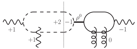
Figure 1: An illustration of the mechanism giving rise to $\cos 3\phi$ azimuthal asymmetry. The solid line represents the quark propagator, while the pion propagator is indicated by the dashed line.

II numerical estimations

We now introduce all ingredients that are necessary for numerical calculations. Most of them follow our previous work Xing et al. (2020). We first introduce the parametrization for the $b_{\perp}$ dependent dipole-nucleus and dipole-nucleon scattering amplitudes. For the dipole-nucleus scattering amplitude, we adopt the parametrization Kowalski and Teaney (2003); Kowalski et al. (2006),

$$N(b_{\perp},r_{\perp})=1-e^{-2\pi B_{p}AT_{A}(b_{\perp}){\cal N}(r_{\perp})}$$ (9)

Here the nuclear thickness function $T_{A}(b_{\perp})$ is computed with the Woods-Saxon distribution, and $B_{p}=4{\text{ GeV}}^{2}$ in the IPsat model. For the dipole-nucleon scattering amplitude, we adopt a conventional parameterization, namely, the GBW model Golec-Biernat and Wusthoff (1998, 1999): ${\cal N}(r_{\perp})=1-e^{-\frac{Q_{s}^{2}r_{\perp}^{2}}{4}}$. For the scalar part of vector meson wave function, we use ”Gaus-LC” wave function also taken from Ref. Kowalski and Teaney (2003); Kowalski et al. (2006).

$$\Phi^{*}(|r_{\perp}|,z)=\beta z(1-z)\exp\left[-\frac{r_{\perp}^{2}}{2R_{\perp}^{2}}\right]$$ (10)

with $\beta=4.47$, $R_{\perp}^{2}=21.9\ \text{GeV}^{-2}$ for $\rho$ meson.

${\cal F}(x,k_{\perp})$ describes the probability amplitude for finding a photon carries certain momentum. The squared ${\cal F}(x,k_{\perp})$ is just the standard photon TMD distribution $f(x,k_{\perp})$. At low transverse momentum it can be commonly computed with the equivalent photon approximation(also often referred to as the Weizs$\ddot{a}$cker-Williams method) which has been widely used to compute UPC observables(see for example Klein et al. (2019); Zha et al. (2020); Klein et al. (2020)). In the equivalent photon approximation, ${\cal F}(x,k_{\perp})$ reads,

$${\cal F}(x,k_{\perp})=\frac{Z\sqrt{\alpha_{e}}}{\pi}|k_{\perp}|\frac{F(k_{\perp}^{2}+x^{2}M_{p}^{2})}{(k_{\perp}^{2}+x^{2}M_{p}^{2})}$$ (11)

where $x$ is constrained according to $x=\sqrt{\frac{P_{\perp}^{2}+m_{\pi}^{2}}{S}}(e^{y_{1}}+e^{y_{2}})$. $M_{p}$ is proton mass. $F$ is the nuclear charge form factor which is assumed to take the Woods-Saxon distribution as well,

$$F(\vec{k}^{2})=\int d^{3}re^{i\vec{k}\cdot\vec{r}}\frac{C^{0}}{1+\exp{\left[(r-R_{A})/d\right]}}$$ (12)

where $R_{A}$(Au: 6.38 fm, pb: 6.62 fm) is the radius and d(Au:0.535 fm, Pb:0.546 fm) is the skin depth. $C^{0}$ is a normalization factor.

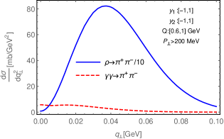
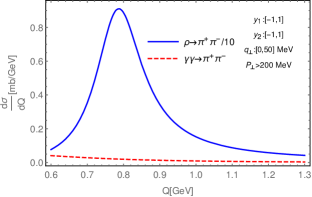
Figure 2: The unpolarized differential cross section as the function of $q_{\perp}$(left panel) and the invariant mass(right panel). The photonuclear cross section $d\sigma_{\rho\rightarrow\pi\pi}$ is rescaled by a factor 1/10.

UPC events are usually triggered at RHIC and LHC by detecting neutrons emitted at forward angles from a scattered nuclei. The probability for emitting a neutron is strongly dependent of the impact parameter. To account for this effect, one should integrate the differential cross section over impact parameter range from $2R_{A}$ to $\infty$ with a weight function,

$$2\pi\int_{2R_{A}}^{\infty}\tilde{b}_{\perp}d\tilde{b}_{\perp}P^{2}(\tilde{b}_{\perp})d\sigma(\tilde{b}_{\perp},\ ...)$$ (13)

where the probability $P(\tilde{b}_{\perp})$ of emitting a neutron from the scattered nucleus is conventionally parameterized as Baur et al. (1998) $P(\tilde{b}_{\perp})=P_{1n}(\tilde{b}_{\perp})\exp\left[-P_{1n}(\tilde{b}_{\perp})\right]$ which is denoted as the “1” event, while for emitting any number of neutrons (“X” event), the probability is given by $P(\tilde{b}_{\perp})=1-\exp\left[-P_{1n}(\tilde{b}_{\perp})\right]$ with $P_{1n}(\tilde{b}_{\perp})=5.45*10^{-5}\frac{Z^{3}(A-Z)}{A^{2/3}\tilde{b}_{\perp}^{2}}\ \text{fm}^{2}$. All the subsequent numerical estimations are made for the “Xn” event. Having all these parameters specified, we are now ready to perform numerical calculation of the azimuthal asymmetries for dipion production in UPCs.

We first present the contributions from the EM interaction and the photonuclear reaction to the azimuthal averaged cross section as the function of the invariant mass and pair transverse momentum in Fig.2. One can see that the EM contribution is not negligible at low transverse momentum and in the low invariant mass region. It is worthy to emphasize again that the interference term drops out in the azimuthal averaged cross section. The suppression of the unpolarized cross section at low $q_{\perp}<40$ MeV is due to the destructive interference that was first discussed in Ref. Klein and Nystrand (2000).

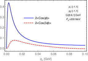
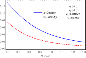
Figure 3: $\cos\phi$ and $\cos 3\phi$ azimuthal asymmetries as the function of $q_{\perp}$(left panel) and the invariant mass(right panel).

The azimuthal asymmetries from the interference term are displayed in Fig. 3, where the asymmetries, i.e. the average value of $\cos 3\phi$ and $\cos\phi$ are defined as,

$$\langle\cos(n\phi)\rangle=\frac{\int\frac{d\sigma}{d{\cal P.S.}}\cos n\phi\ d{\cal P.S.}}{\int\frac{d\sigma}{d{\cal P.S.}}d{\cal P.S.}}$$ (14)

with $n=1,3$. These asymmetries are calculated at the RHIC energy $\sqrt{S}=200{\text{ GeV}}$. Both $\langle\cos\phi\rangle$ and $\langle\cos 3\phi\rangle$ reach the maximal value at very low $q_{\perp}$ and then start to decrease with increasing $q_{\perp}$. They remain sizable and are roughly few percentage level in the transverse momentum region $20\ {\text{MeV}}<q_{\perp}<60{\text{ MeV}}$. The analysing power is basically of the same order of that from the helicity flip amplitude in elastic proton-proton scatterings, where the interference at low transverse momentum between the EM and hadronic contributions has long been used as a tool in the study of the phase of the hadronic amplitude Buttimore et al. (1978, 1999) (see also a recent development Hagiwara et al. (2020) ).

III conclusion

In summary, we have studied the $\cos\phi$ and $\cos 3\phi$ azimuthal angular correlations in exclusive $\pi^{+}\pi^{-}$ pair production near $\rho^{0}$ resonance peak in ultraperipheral heavy ion collisions, where $\phi$ is defined as the angle between pion’s transverse momentum and pair’s transverse momentum. The asymmetry essentially results from the linear polarization of incident coherent photons. We focus on low pair transverse momentum where the electromagnetic and nuclear amplitudes of dipion production are comparable. In this work, we demonstrate that $\cos\phi$ and $\cos 3\phi$ azimuthal asymmetries are the characteristic signals of the CNI effect in exclusive pion pair production in UPCs. These azimuthal asymmetries are shown to be sizable in the kinematic region of interest, thus can serve as an alternative method to constrain the phase of the dipole amplitude. It should be feasible to measure the proposed observables at RHIC and LHC. We notice that the direct pion pair continuum receives contributions from several different channels Soding (1966); Brodsky et al. (1971); Klusek-Gawenda and Szczurek (2013); Bolz et al. (2015). Though they unlikely dominate low pair transverse momentum spectrum, it would be interesting to carry out a more comprehensive analysis in a future publication.

References

Ryskin (1993)
M. Ryskin, Z.
Phys. C 57, 89
(1993).
Brodsky et al. (1994)
S. J. Brodsky,
L. Frankfurt,
J. Gunion,
A. H. Mueller,
and M. Strikman,
Phys. Rev. D 50,
3134 (1994), eprint hep-ph/9402283.
Klein and Nystrand (1999)
S. Klein and
J. Nystrand,
Phys. Rev. C 60,
014903 (1999), eprint hep-ph/9902259.
Munier et al. (2001)
S. Munier,
A. Stasto, and
A. H. Mueller,
Nucl. Phys. B 603,
427 (2001), eprint hep-ph/0102291.
Kowalski and Teaney (2003)
H. Kowalski and
D. Teaney,
Phys. Rev. D 68,
114005 (2003), eprint hep-ph/0304189.
Kowalski et al. (2006)
H. Kowalski,
L. Motyka, and
G. Watt,
Phys. Rev. D 74,
074016 (2006), eprint hep-ph/0606272.
Strikman (2008)
M. Strikman,
Nucl. Phys. B Proc. Suppl.
179-180, 111
(2008).
Rebyakova et al. (2012)
V. Rebyakova,
M. Strikman, and
M. Zhalov,
Phys. Lett. B 710,
647 (2012), eprint 1109.0737.
Guzey and Zhalov (2013)
V. Guzey and
M. Zhalov,
JHEP 10, 207
(2013), eprint 1307.4526.
Lappi and Mantysaari (2011)
T. Lappi and
H. Mantysaari,
Phys. Rev. C 83,
065202 (2011), eprint 1011.1988.
Xie and Chen (2016)
Y.-p. Xie and
X. Chen,
Eur. Phys. J. C 76,
316 (2016), eprint 1602.00937.
Cai et al. (2020)
Y. Cai,
W. Xiang,
M. Wang, and
D. Zhou,
Chin. Phys. C 44,
074110 (2020), eprint 2002.12610.
Hagiwara et al. (2017)
Y. Hagiwara,
Y. Hatta,
R. Pasechnik,
M. Tasevsky, and
O. Teryaev,
Phys. Rev. D 96,
034009 (2017), eprint 1706.01765.
Hatta et al. (2020)
Y. Hatta,
M. Strikman,
J. Xu, and
F. Yuan,
Phys. Lett. B 803,
135321 (2020), eprint 1911.11706.
Khachatryan et al. (2017)
V. Khachatryan
et al. (CMS), Phys.
Lett. B 772, 489
(2017), eprint 1605.06966.
Adamczyk et al. (2017)
L. Adamczyk et al.
(STAR), Phys. Rev. C
96, 054904
(2017), eprint 1702.07705.
Adam et al. (2019a)
J. Adam et al.
(STAR), Phys. Rev. Lett.
123, 132302
(2019a), eprint 1904.11658.
Sirunyan et al. (2019)
A. M. Sirunyan
et al. (CMS), Eur.
Phys. J. C 79, 702
(2019), eprint 1902.01339.
Acharya et al. (2020)
S. Acharya et al.
(ALICE), JHEP
06, 035 (2020),
eprint 2002.10897.
Soding (1966)
P. Soding,
Phys. Lett. 19,
702 (1966).
Brodsky et al. (1971)
S. J. Brodsky,
T. Kinoshita,
and H. Terazawa,
Phys. Rev. D 4,
1532 (1971).
Klusek-Gawenda and
Szczurek (2013)
M. Klusek-Gawenda
and A. Szczurek,
Phys. Rev. C 87,
054908 (2013), eprint 1302.4204.
Bolz et al. (2015)
A. Bolz,
C. Ewerz,
M. Maniatis,
O. Nachtmann,
M. Sauter, and
A. Schöning,
JHEP 01, 151
(2015), eprint 1409.8483.
Li et al. (2019)
C. Li,
J. Zhou, and
Y.-J. Zhou,
Phys. Lett. B 795,
576 (2019), eprint 1903.10084.
Li et al. (2020)
C. Li,
J. Zhou, and
Y.-J. Zhou,
Phys. Rev. D 101,
034015 (2020), eprint 1911.00237.
Xiao et al. (2020)
B.-W. Xiao,
F. Yuan, and
J. Zhou
(2020), eprint 2003.06352.
Adam et al. (2019b)
J. Adam et al.
(STAR) (2019b),
eprint 1910.12400.
Brandenburg et al. (2019)
J. D. Brandenburg
et al. (STAR), talk
presented in Quark Matter 2019, Wuhan, China (2019).
Xing et al. (2020)
H. Xing,
C. Zhang,
J. Zhou, and
Y.-J. Zhou,
JHEP 10, 064
(2020), eprint 2006.06206.
Klein and Nystrand (2000)
S. R. Klein and
J. Nystrand,
Phys. Rev. Lett. 84,
2330 (2000), eprint hep-ph/9909237.
Abelev et al. (2009)
B. Abelev et al.
(STAR), Phys. Rev. Lett.
102, 112301
(2009), eprint 0812.1063.
Zha et al. (2019)
W. Zha,
L. Ruan,
Z. Tang,
Z. Xu, and
S. Yang,
Phys. Rev. C 99,
061901 (2019), eprint 1810.10694.
Klein et al. (2020)
S. Klein,
A. Mueller,
B.-W. Xiao, and
F. Yuan
(2020), eprint 2003.02947.
Sun et al. (2020)
Z.-h. Sun,
D.-x. Zheng,
J. Zhou, and
Y.-j. Zhou,
Phys. Lett. B 808,
135679 (2020), eprint 2002.07373.
Golec-Biernat and
Wusthoff (1998)
K. J. Golec-Biernat
and M. Wusthoff,
Phys. Rev. D 59,
014017 (1998), eprint hep-ph/9807513.
Golec-Biernat and
Wusthoff (1999)
K. J. Golec-Biernat
and M. Wusthoff,
Phys. Rev. D 60,
114023 (1999), eprint hep-ph/9903358.
Klein et al. (2019)
S. Klein,
A. Mueller,
B.-W. Xiao, and
F. Yuan,
Phys. Rev. Lett. 122,
132301 (2019), eprint 1811.05519.
Zha et al. (2020)
W. Zha,
J. D. Brandenburg,
Z. Tang, and
Z. Xu, Phys.
Lett. B 800, 135089
(2020), eprint 1812.02820.
Baur et al. (1998)
G. Baur,
K. Hencken, and
D. Trautmann,
J. Phys. G 24,
1657 (1998), eprint hep-ph/9804348.
Buttimore et al. (1978)
N. H. Buttimore,
E. Gotsman, and
E. Leader,
Phys. Rev. D 18,
694 (1978), [Erratum:
Phys.Rev.D 35, 407 (1987)].
Buttimore et al. (1999)
N. H. Buttimore,
B. Kopeliovich,
E. Leader,
J. Soffer, and
T. Trueman,
Phys. Rev. D 59,
114010 (1999), eprint hep-ph/9901339.
Hagiwara et al. (2020)
Y. Hagiwara,
Y. Hatta,
R. Pasechnik,
and J. Zhou,
Eur. Phys. J. C 80,
427 (2020), eprint 2003.03680.