Regret Bounds for Adaptive Nonlinear Control

Abstract

We study the problem of adaptively controlling a known discrete-time nonlinear system subject to unmodeled disturbances. We prove the first finite-time regret bounds for adaptive nonlinear control with matched uncertainty in the stochastic setting, showing that the regret suffered by certainty equivalence adaptive control, compared to an oracle controller with perfect knowledge of the unmodeled disturbances, is upper bounded by $\widetilde{O}(\sqrt{T})$ in expectation. Furthermore, we show that when the input is subject to a $k$ timestep delay, the regret degrades to $\widetilde{O}(k\sqrt{T})$. Our analysis draws connections between classical stability notions in nonlinear control theory (Lyapunov stability and contraction theory) and modern regret analysis from online convex optimization. The use of stability theory allows us to analyze the challenging infinite-horizon single trajectory setting.

1 Introduction

The goal of adaptive nonlinear control (Slotine and Li, 1991; Ioannou and Sun, 1996; Fradkov et al., 1999) is to control a continuous-time dynamical system in the presence of unknown dynamics; it is the study of concurrent learning and control of dynamical systems. There is a rich body of literature analyzing the stability and convergence properties of classical adaptive control algorithms. Under suitable assumptions (e.g., Lyapunov stability of the known part of the system), typical results guarantee asymptotic convergence of the unknown system to a fixed point or desired trajectory.

On the other hand, due to recent successes of reinforcement learning (RL) in the control of physical systems (Yang et al., 2019; OpenAI et al., 2019; Hwangbo et al., 2019; Williams et al., 2017; Levine et al., 2016), there has been a flurry of research in online RL algorithms for continuous control. In contrast to the classical setting of adaptive nonlinear control, online RL algorithms operate in discrete-time, and often come with finite-time regret bounds (Wang et al., 2019; Kakade et al., 2020; Jin et al., 2020; Cao and Krishnamurthy, 2020; Cai et al., 2020; Agarwal et al., 2020). These bounds provide a quantitative rate at which the control performance of the online algorithm approaches the performance of an oracle equipped with hindsight knowledge of the uncertainty.

In this work, we revisit the analysis of adaptive nonlinear control algorithms through the lens of modern reinforcement learning. Specifically, we show how to systematically port matched uncertainty adaptive control algorithms to discrete-time, and we use the machinery of online convex optimization (Hazan, 2016) to prove finite-time regret bounds. Our analysis uses the notions of contraction and incremental stability (Lohmiller and Slotine, 1998; Angeli, 2002) to draw a connection between control regret, the quantity we are interested in, and function prediction regret, the quantity online convex optimization enables us to bound.

We present two main sets of results. First, we provide a discrete-time analysis of velocity gradient adaptation (Fradkov et al., 1999), a broad framework which encompasses e.g., classic adaptive sliding control (Slotine and Coetsee, 1986). We prove that in the deterministic setting, if a Lyapunov function describing the nominal system is strongly convex in the state, then the corresponding velocity gradient algorithm achieves constant regret with respect to a baseline controller having full knowledge of the system. Our second line of results considers the use of online least-squares gradient based optimization for the parameters. Under an incremental input-to-state stability assumption, we prove $\widetilde{O}(\sqrt{T})$ regret bounds in the presence of stochastic process noise. We further show that when the input is delayed by $k$ timesteps, the regret degrades to $\widetilde{O}(k\sqrt{T})$. Importantly, our bounds hold for the challenging single trajectory infinite horizon setting, rather than the finite-horizon episodic setting more frequently studied in reinforcement learning. We conclude with simulations showing the efficacy of our proposed discrete-time algorithms in quickly adapting to unmodeled disturbances.

2 Related Work

There has been a renewed focus on the continuous state and action space setting in the reinforcement learning (RL) literature. The most well-studied problem for continuous control in RL is the Linear Quadratic Regulator (LQR) problem with unknown dynamics. For LQR, both upper and lower bounds achieving $\sqrt{T}$ regret are available (Abbasi-Yadkori and Szepesvári, 2011; Agarwal et al., 2019a; Mania et al., 2019; Cohen et al., 2019; Simchowitz and Foster, 2020; Hazan et al., 2020), for stochastic and adversarial noise processes. Furthermore, in certain settings it is even possible to obtain logarithmic regret (Agarwal et al., 2019b; Cassel et al., 2020; Foster and Simchowitz, 2020).

Results that extend beyond the classic LQR problem are less complete, but are rapidly growing. Recently, Kakade et al. (2020) showed $\sqrt{T}$ regret bounds in the finite horizon episodic setting for dynamics of the form $x_{t+1}=A\phi(x_{t},u_{t})+w_{t}$ where $A$ is an unknown operator and $\phi$ is a known feature map, though their algorithm is generally not tractable to implement. Mania et al. (2020) show how to actively recover the parameter matrix $A$ using trajectory optimization. Azizzadenesheli et al. (2018); Jin et al. (2020); Yang and Wang (2020); Zanette et al. (2020) show $\sqrt{T}$ regret bounds for linear MDPs, which implies that the associated $Q$-function is linear after a known feature transformation. Wang et al. (2019) extend this model to allow for generalized linear model $Q$-functions. Unlike the stability notions considered in this work, we are unaware of any algorithmic method of verifying the linear MDP assumption. Furthermore, the aforementioned regret bounds are for the finite-horizon episodic setting; we study the infinite-horizon single trajectory setting without resets.

Very few results categorizing regret bounds for adaptive nonlinear control exist; one recent example is Gaudio et al. (2019), who highlight that simple model reference adaptive controllers obtain constant regret in the continuous-time deterministic setting. In contrast, our work simultaneously tackles the issues of more general models, discrete-time systems, and stochastic noise. We note that several authors have ported various adaptive controllers into discrete-time (Pieper, 1996; Bartolini et al., 1995; Loukianov et al., 2018; Muñoz and Sbarbaro, 2000; Kanellakopoulos, 1994; Ordóñez et al., 2006). These results, however, are mostly concerned with asymptotic stability of the closed-loop system, as opposed to finite-time regret bounds.

3 Problem Statement

In this work, we focus on the following discrete-time, time-varying, and nonlinear dynamical system with linearly parameterized unknown in the matched uncertainty setting:

$$x_{t+1}=f(x_{t},t)+B(x_{t},t)(u_{t}-Y(x_{t},t)\alpha)+w_{t}\>.$$ (3.1)

Here $x_{t}\in\mathbb{R}^{n}$, $u_{t}\in\mathbb{R}^{d}$, $f:\mathbb{R}^{n}\times\mathbb{N}\rightarrow\mathbb{R}^{n}$ is a known nominal dynamics model, $B:\mathbb{R}^{n}\times\mathbb{N}\rightarrow\mathbb{R}^{n\times d}$ is a known input matrix, $Y:\mathbb{R}^{n}\times\mathbb{N}\rightarrow\mathbb{R}^{d\times p}$ is a matrix of known basis functions, and $\alpha\in\mathbb{R}^{p}$ is a vector of unknown parameters. The sequence of noise vectors $\{w_{t}\}\subseteq\mathbb{R}^{n}$ is assumed to satisfy the distributional requirements $\mathbb{E}[w_{t}]=0$, $\lVert w_{t}\rVert\leqslant W$ almost surely, and that $w_{s}$ is independent of $w_{t}$ for all $s\neq t$. We further assume that $\alpha\in\mathcal{C}:=\{\alpha\in\mathbb{R}^{p}:\lVert\alpha\rVert\leqslant D\}$, and that an upper bound for $D$ is known. Without loss of generality, we set the origin to be a fixed-point of the nominal dynamics, so that $f(0,t)=0$ for all $t$. Because the nominal dynamics is time-varying, this formalism captures the classic setting of nonlinear adaptive control, which considers the problem of tracking a time-varying desired trajectory $x^{d}_{t}$.

We study certainty equivalence controllers. In particular, we maintain a parameter estimate $\hat{\alpha}_{t}\in\mathcal{C}$ and play the input $u_{t}=Y(x_{t},t)\hat{\alpha}_{t}$. Our goal is to design a learning algorithm that updates $\hat{\alpha}_{t}$ to cancel the unknown and which provides a guarantee of fast convergence to the performance of an ideal comparator. The comparator that we will study is an oracle that plays the ideal control $u_{t}=Y(x_{t},t)\alpha$ at every timestep, leading to the dynamics $x_{t+1}=f(x_{t},t)+w_{t}$. To measure the rate of convergence to this comparator, we study the following notion of control regret:

$$\mathsf{Regret}(T):=\mathbb{E}_{\{w_{t}\}}\left[\sum_{t=0}^{T-1}\lVert x_{t}^{a}\rVert^{2}-\lVert x_{t}^{c}\rVert^{2}\right]\>.$$ (3.2)

Here, the trajectory $\{x_{t}^{a}\}$ is generated by an adaptive control algorithm, while the trajectory $\{x_{t}^{c}\}$ is generated by the oracle with access to the true parameters $\alpha$. Our notation for $x_{t}^{a}$ and $x_{t}^{c}$ suppresses the dependence of the trajectory on the noise sequence $\{w_{t}\}$. Our goal will be to design algorithms that exhibit sub-linear regret, i.e., $\mathsf{Regret}(T)=o(T)$, which ensures that the time-averaged regret asymptotically converges to zero. For ease of exposition, in the sequel we define $Y_{t}:=Y(x_{t}^{a},t)$ and $B_{t}:=B(x_{t}^{a},t)$, and we use the symbol $\tilde{\alpha}_{t}$ to denote the parameter estimation error $\ \hat{\alpha}_{t}-\alpha$.

3.1 Parameter Update Algorithms

We study two primary classes of parameter update algorithms inspired by online convex optimization (Hazan, 2016). The first is the family of velocity gradient algorithms (Fradkov et al., 1999), which perform online gradient-based optimization on a Lyapunov function for the nominal system. The second obviates the need for a known Lyapunov function, and directly performs online optimization on the least-squares prediction error. Here we discuss the discrete-time formulation, but a self-contained introduction to these algorithms in continuous-time can be found in Appendix A.

3.1.1 Velocity gradient algorithms

Velocity gradient algorithms exploit access to a known Lyapunov function for the nominal dynamics. Specifically, assume the existence of a non-negative function $Q(x,t):\mathbb{R}^{n}\times\mathbb{N}\rightarrow\mathbb{R}_{\geqslant 0}$, which is differentiable in its first argument, and a constant $\rho\in(0,1)$ such that for all $x,t$:

$$Q(f(x,t),t+1)\leqslant Q(x,t)-\rho\lVert x\rVert^{2}\>.$$ (3.3)

Given such a $Q(x,t)$, velocity gradient methods update the parameters according to the iteration

$$\hat{\alpha}_{t+1}=\Pi_{\mathcal{C}}[\hat{\alpha}_{t}-\eta_{t}Y(x_{t},t)^{\mathsf{T}}B(x_{t},t)^{\mathsf{T}}\nabla Q(x_{t+1},t+1)]\>,\>\>\Pi_{\mathcal{C}}[x]:=\arg\min_{y\in\mathcal{C}}\lVert x-y\rVert\>,$$ (3.4)

which can alternatively be viewed as projected gradient descent with respect to the parameters after noting that $Y(x_{t},t)^{\mathsf{T}}B(x_{t},t)^{\mathsf{T}}\nabla Q(x_{t+1},t+1)=\nabla_{\hat{\alpha}_{t}}Q(x_{t+1},t+1)$. As we will demonstrate, the use of $\nabla Q(x_{t+1},t+1)$ instead of $\nabla Q(x_{t},t)$ in (3.4) is key to unlocking a sublinear regret bound.

3.1.2 Online least-squares

Online least-squares algorithms are motivated by minimizing the approximation error directly rather than through stability considerations. For each time $t$, define the prediction error loss function

$$f_{t}(\hat{\alpha}):=\frac{1}{2}\lVert B(x_{t},t)Y(x_{t},t)(\hat{\alpha}-\alpha)+w_{t}\rVert^{2}\>.$$ (3.5)

Unlike in the usual optimization setting, the loss at time $t$ is unknown to the controller, due to its dependence on the unknown parameters $\alpha$. However, its gradient $\nabla f_{t}(\hat{\alpha}_{t})$ can be implemented after observing $x_{t+1}$ through a discrete-time analogue of Luenberger’s well-known approach for reduced-order observer design (Luenberger, 1979):

$$\nabla f_{t}(\hat{\alpha}_{t})=Y(x_{t},t)^{\mathsf{T}}B(x_{t},t)^{\mathsf{T}}(x_{t+1}-f(x_{t},t))\>.$$ (3.6)

The simplest update rule that uses the gradient $\nabla f_{t}(\hat{\alpha}_{t})$ is online gradient descent:

$$\hat{\alpha}_{t+1}=\Pi_{\mathcal{C}}[\hat{\alpha}_{t}-\eta_{t}\nabla f_{t}(\hat{\alpha}_{t})]\>,$$ (3.7)

while a more sophisticated update rule is the online Newton method:

$$\hat{\alpha}_{t+1}=\Pi_{\mathcal{C},t}[\hat{\alpha}_{t}-\eta A_{t}^{-1}\nabla f_{t}(\hat{\alpha}_{t})]\>,\>\>A_{t}=\lambda I+\sum_{s=0}^{t}M_{s}^{\mathsf{T}}M_{s}\>,\>\>M_{s}=B(x_{s},s)Y(x_{s},s)\>.$$ (3.8)

Above, the operator $\Pi_{\mathcal{C},t}[\cdot]$ denotes projection w.r.t. the $A_{t}$-norm: $\Pi_{\mathcal{C},t}[x]:=\arg\min_{y\in\mathcal{C}}\lVert x-y\rVert_{A_{t}}$.

4 Regret Bounds for Velocity Gradient Algorithms

In this section, we provide a regret analysis for the velocity gradient algorithm. Here, we will assume a deterministic system, so that $w_{t}\equiv 0$. Unrolling the Lyapunov stability assumption (3.3) and using the non-negativity of $Q(x,t)$ yields $\sum_{t=0}^{T-1}\lVert x_{t}^{c}\rVert^{2}\leqslant\frac{Q(x_{0},0)}{\rho}$, which shows that the contribution of $\sum_{t=0}^{T-1}\lVert x_{t}^{c}\rVert^{2}$ to the regret is $O(1)$. Therefore, it suffices to bound $\sum_{t=0}^{T-1}\lVert x_{t}^{a}\rVert^{2}$ directly. The key assumption that enables application of the velocity gradient method in discrete-time is strong convexity of the Lyapunov function $Q(x,t)$ with respect to $x$. Recall that a $C^{1}$ function $h(x)$ is $\mu$-strongly convex if for all $x$ and $y$, $h(y)\geqslant h(x)+\langle\nabla h(x),y-x\rangle+\frac{\mu}{2}\lVert y-x\rVert^{2}$. Our first result is a data-dependent regret bound for the velocity gradient algorithm.

Theorem 4.1.

Fix a $\lambda>0$. Consider the velocity gradient update (3.4) with $\hat{\alpha}_{0}\in\mathcal{C}$ and learning rate $\eta_{t}=\frac{D}{\sqrt{\lambda+\sum_{i=0}^{t}\lVert Y_{i}^{\mathsf{T}}B_{i}^{\mathsf{T}}\nabla Q(x_{i+1}^{a},i+1)\rVert^{2}}}$. Assume that the Lyapunov stability condition (3.3) is verified, and that for every $t$, the map $x\mapsto Q(x,t)$ is $\mu$-strongly convex. Then for any $T\geqslant 1$:

$$\sum_{t=0}^{T-1}\lVert x_{t}^{a}\rVert^{2}+\frac{\mu}{2\rho}\sum_{t=0}^{T-1}\lVert B_{t}Y_{t}\tilde{\alpha}_{t}\rVert^{2}\leqslant\frac{Q(x_{0},0)}{\rho}+\frac{5\sqrt{\lambda}D}{\rho}+\frac{3D}{\rho}\sqrt{\sum_{t=0}^{T-1}\lVert Y_{t}^{\mathsf{T}}B_{t}^{\mathsf{T}}\nabla Q(x_{t+1}^{a},t+1)\rVert^{2}}\>.$$

By Theorem 4.1, a bound on $\sum_{t=0}^{T-1}\lVert Y_{t}^{\mathsf{T}}B_{t}^{\mathsf{T}}\nabla Q(x_{t+1}^{a},t+1)\rVert^{2}$ ensures a bound on the control regret. One way to obtain a bound is to assume that $\lVert Y_{t}^{\mathsf{T}}B_{t}^{\mathsf{T}}\nabla Q(x_{t+1}^{a},t+1)\rVert\leqslant G$ for all $t$, in which case Theorem 4.1 yields the sublinear guarantee $\mathsf{Regret}(T)\leqslant O(\sqrt{T})$. However, this can be strengthened by assuming that both $\nabla Q(x,t)$ and $f(x,t)$ are Lipschitz continuous.

Theorem 4.2.

Suppose that for every $x$ and $t$, $\lVert\nabla Q(x,t)\rVert\leqslant L_{Q}\lVert x\rVert$ and $\lVert f(x,t)\rVert\leqslant L_{f}\lVert x\rVert$. Further assume that $\sup_{x,t}\lVert B(x,t)\rVert\leqslant M$ and $\sup_{x,t}\lVert Y(x,t)\rVert\leqslant M$. Then, under the hypotheses of Theorem 4.1, for any $T\geqslant 1$:

$$\sum_{t=0}^{T-1}\lVert x_{t}^{a}\rVert^{2}+\frac{\mu}{2\rho}\sum_{t=0}^{T-1}\lVert B_{t}Y_{t}\tilde{\alpha}_{t}\rVert^{2}\leqslant\frac{3}{2}\left(\frac{Q(x_{0},0)}{\rho}+\frac{5\sqrt{\lambda}D}{\rho}\right)+\frac{27D^{2}}{\rho^{2}}M^{4}L_{Q}^{2}\max\left\{L_{f}^{2},\frac{2\rho}{\mu}\right\}\>.$$

Theorem 4.2 yields the constant bound $\mathsf{Regret}(T)\leqslant O(1)$, which mirrors an earlier result in the continuous-time deterministic setting due to Gaudio et al. (2019).

5 Regret Bounds for Online Least-Squares Algorithms

In this section we study the use of online least-squares algorithms for adaptive control in the stochastic setting. A core challenge in this setting is that neither $\mathbb{E}\sum_{t=0}^{T-1}\lVert x_{t}^{a}\rVert^{2}$ nor $\mathbb{E}\sum_{t=0}^{T-1}\lVert x_{t}^{c}\rVert^{2}$ converges to a constant, but rather each grows as $\Omega(T)$. Any analysis yielding a sublinear regret bound must therefore consider the behavior of the trajectory $x_{t}^{a}$ together with the trajectory $x_{t}^{c}$, and cannot bound the two terms independently. Our approach couples the trajectories together with the same noise realization $\{w_{t}\}$, and then utilizes incremental stability to compare trajectories of the comparator and the adaptation algorithm. We first provide a brief introduction to contraction and incremental stability, and then we discuss our results.

5.1 Contraction and Incremental Stability

To prove regret bounds for our least-squares algorithms, we use the following generalization of input-to-state stability, which allows for a direct comparison between two trajectories of the system in terms of the strength of past inputs.

Definition 5.1 (cf. Angeli (2002)).

Let constants $\beta,\gamma$ be positive and $\rho\in(0,1)$. The discrete-time dynamical system $f(x,t)$ is called $(\beta,\rho,\gamma)$-exponentially-incrementally-input-to-state-stable (E-$\delta$ISS) for a pair of initial conditions $(x_{0},y_{0})$ and signal $u_{t}$ (which is possibly adapted to the history $\{x_{s}\}_{s\leqslant t}$) if the trajectories $x_{t+1}=f(x_{t},t)+u_{t}$ and $y_{t+1}=f(y_{t},t)$ satisfy for all $t\geqslant 0$:

$$\lVert x_{t}-y_{t}\rVert\leqslant\beta\rho^{t}\lVert x_{0}-y_{0}\rVert+\gamma\sum_{k=0}^{t-1}\rho^{t-1-k}\lVert u_{k}\rVert\>.$$ (5.1)

A system is $(\beta,\rho,\gamma)$-E-$\delta$ISS if it is $(\beta,\rho,\gamma)$-E-$\delta$ISS for all initial conditions $(x_{0},y_{0})$ and signals $u_{t}$.

Definition 5.1 can be verified by checking if the system $f(x,t)$ is contracting.

Definition 5.2 (cf. Lohmiller and Slotine (1998)).

The discrete-time dynamical system $f(x,t)$ is contracting with rate $\gamma\in(0,1)$ in the metric $M(x,t)$ if for all $x$ and $t$:

$$\frac{\partial f}{\partial x}(x,t)^{\mathsf{T}}M(f(x,t),t+1)\frac{\partial f}{\partial x}(x,t)\preccurlyeq\gamma M(x,t)\>.$$

Proposition 5.3.

Let $f(x,t)$ be contracting with rate $\gamma\in(0,1)$ in the metric $M(x,t)$. Assume that for all $x,t$ we have $0\prec\mu I\preccurlyeq M(x,t)\preccurlyeq LI$. Then $f(x,t)$ is $(\sqrt{L/\mu},\sqrt{\gamma},\sqrt{L/\mu})$-E-$\delta$ISS.

Furthermore, contraction is robust to small perturbations – if the dynamics $f(x,t)$ are contracting, so are the dynamics $f(x,t)+w_{t}$ for small enough $w_{t}$.

Proposition 5.4.

Let $\{w_{t}\}$ be a fixed sequence satisfying $\sup_{t\geqslant 0}\lVert w_{t}\rVert\leqslant W$. Suppose that $f(x,t)$ is contracting with rate $\gamma$ in the metric $M(x,t)$ with $M(x,t)\succcurlyeq\mu I$. Define the perturbed dynamics $g(x,t):=f(x,t)+w_{t}$. Suppose that for all $t$, the function $x\mapsto M(x,t)$ is $L_{M}$-Lipschitz. Furthermore, suppose that $\sup_{x,t}\lVert\frac{\partial f}{\partial x}(x,t)\rVert\leqslant L_{f}$. Then as long as $W\leqslant\frac{\mu(1-\gamma)}{L_{f}^{2}L_{M}}$, we have that $g(x,t)$ is contracting with rate $\gamma+\frac{L_{f}^{2}L_{M}W}{\mu}$ in the metric $M(x,t)$.

Note that if the metric is state independent (i.e., $M(x,t)=M(t)$), then we can take $L_{M}=0$ and hence the perturbed system $g(x,t)$ is contracting at rate $\gamma$ for all realizations $\{w_{t}\}$.

5.2 Main Results

Our analysis proceeds by assuming that for almost all noise realizations $\{w_{t}\}$, the perturbed nominal system $f(x,t)+w_{t}$ is incrementally stable (E-$\delta$ISS). We apply incremental stability to bound the control regret directly in terms of the prediction regret, $\mathsf{Regret}(T)\leqslant O(\sqrt{T}\sqrt{\sum_{t=0}^{T-1}\mathbb{E}\lVert B_{t}Y_{t}\tilde{\alpha}_{t}\rVert^{2}})$. Because online convex optimization methods provide explicit guarantees on the prediction regret, we can apply existing results from the online optimization literature to generate a bound on the control regret. To see this, recall that the sequence of prediction error functions $\{f_{t}\}$ from (3.5) has the form $f_{t}(\hat{\alpha})=\frac{1}{2}\lVert B_{t}Y_{t}(\hat{\alpha}-\alpha)+w_{t}\rVert^{2}$. Hence:

$$\frac{1}{2}\mathbb{E}\sum_{t=0}^{T-1}\lVert B_{t}Y_{t}\tilde{\alpha}_{t}\rVert^{2}=\mathbb{E}\left[\sum_{t=0}^{T-1}f_{t}(\hat{\alpha}_{t})-f_{t}(\alpha)\right]\leqslant\mathbb{E}\left[\sup_{\alpha\in\mathcal{C}}\sum_{t=0}^{T-1}f_{t}(\hat{\alpha}_{t})-f_{t}(\alpha)\right]\>.$$

In this section, we make the following assumption regarding the dynamics.

Assumption 5.5.

The perturbed system $g(x_{t},t):=f(x_{t},t)+w_{t}$ is $(\beta,\rho,\gamma)$-E-$\delta$ISS for all realizations $\{w_{t}\}$ satisfying $\sup_{t}\lVert w_{t}\rVert\leqslant W$. Also $\sup_{x,t}\lVert B(x,t)\rVert\leqslant M$ and $\sup_{x,t}\lVert Y(x,t)\rVert\leqslant M$.

We define the constant $B_{x}:=\beta\lVert x_{0}\rVert+\frac{\gamma(2DM^{2}+W)}{1-\rho}$ and $G:=M^{2}(2DM^{2}+W)$. A key result, which relates control regret to prediction regret, is given in the following theorem.

Theorem 5.6.

Consider any adaptive update rule $\{\hat{\alpha}_{t}\}$. Under Assumption 5.5, for all $T\geqslant 1$:

$$\mathbb{E}\left[\sum_{t=0}^{T-1}\lVert x_{t}^{a}\rVert^{2}-\lVert x_{t}^{c}\rVert^{2}\right]\leqslant\frac{2B_{x}\gamma}{1-\rho}\sqrt{T}\sqrt{\sum_{t=0}^{T-1}\mathbb{E}\lVert B_{t}Y_{t}\tilde{\alpha}_{t}\rVert^{2}}\>.$$

We can immediately specialize Theorem 5.6 to both online gradient descent and online Newton. Both corollaries are a direct consequence of applying well-known regret bounds in online convex optimization to Theorem 5.6 (cf. Proposition E.1 and Proposition E.2 in Appendix F). Our first corollary shows that online gradient descent achieves a $O(T^{3/4})$ control regret bound.

Corollary 5.7.

Suppose we use online gradient descent (3.7) to update the parameters, setting the learning rate $\eta_{t}=\frac{D}{G\sqrt{t+1}}$. Under Assumption 5.5, for all $T\geqslant 1$:

$$\mathbb{E}\left[\sum_{t=0}^{T-1}\lVert x_{t}^{a}\rVert^{2}-\lVert x_{t}^{c}\rVert^{2}\right]\leqslant 2\sqrt{6}B_{x}\frac{\gamma}{1-\rho}\sqrt{GD}T^{3/4}\>.$$

This result immediately generalizes to the case of mirror descent, where dimension-dependence implicit in $G$ and $D$ can be reduced, and where recent implicit regularization results apply (Boffi and Slotine, 2020). Next, the regret can be improved to $O(\sqrt{T\log{T}})$ by using online Newton.

Corollary 5.8.

Suppose we use the online Newton method (3.8) to update the parameters, setting $\eta=1$. Suppose furthermore that $M\geqslant 1$. Under Assumption 5.5, for all $T\geqslant 1$:

$$\mathbb{E}\left[\sum_{t=0}^{T-1}\lVert x_{t}^{a}\rVert^{2}-\lVert x_{t}^{c}\rVert^{2}\right]\leqslant\frac{2B_{x}\gamma}{1-\rho}\sqrt{T}\sqrt{4D^{2}(\lambda+M^{4})+pG^{2}\log(1+M^{4}T/\lambda)}\>.$$

We also note that in the deterministic setting, online gradient descent to update the parameters achieves $O(1)$ prediction and control regret, which is consistent with the results in Section 4 and with the results in Gaudio et al. (2019). We give a self-contained proof of this in Appendix A.

5.3 Input Delay Results

Motivated by extended matching conditions commonly considered in continuous-time adaptive control (Krstić et al., 1995), we now extend our previous results to a setting where the input is time-delayed by $k$ steps. Specifically, we consider the modified system:

$$x_{t+1}=f(x_{t},t)+B(x_{t},t)(\xi_{t}-Y(t)\alpha)+w_{t}\>,\>\>\xi_{t}=u_{t-k}\>.$$ (5.2)

Here, we simplify part of the model (3.1) by assuming that the matrix $Y(t)$ is state-independent. With this simplification, the certainty equivalence controller is given by $u_{t}=Y(t+k)\hat{\alpha}_{t}$. The baseline we compare to in the definition of regret is the nominal system $x_{t+1}^{c}=f(x_{t}^{c},t)+w_{t}$, which is equivalent to playing the input $u_{t}=Y(t+k)\alpha$. Note that the gradient $\nabla f_{t}(\hat{\alpha}_{t})$ can be implemented by the controller as $\nabla f_{t}(\hat{\alpha}_{t})=Y_{t}^{\mathsf{T}}B_{t}^{\mathsf{T}}(x_{t+1}-f(x_{t},t)-B_{t}(\xi_{t}-Y_{t}\hat{\alpha}_{t}))$.

Folk wisdom and basic intuition suggest that nonlinear adaptive control algorithms for the extended matching setting will perform worse than their matched counterparts; however, standard asymptotic guarantees do not distinguish between the performance of these two classes of algorithms. Here we show that the control regret rigorously captures this gap in performance. We begin with online gradient descent, which provides a regret bound of $O(T^{3/4}+k\sqrt{T})$.

Theorem 5.9.

Consider the online gradient descent update (3.7) for the $k$-step delayed system (5.2) with step size $\eta_{t}=\frac{D}{G\sqrt{t+1}}$. Under Assumption 5.5 and with state-independent $Y_{t}$, for all $T\geqslant k$:

$$\mathbb{E}\left[\sum_{t=0}^{T-1}\lVert x_{t}^{a}\rVert^{2}-\lVert x_{t}^{c}\rVert^{2}\right]\leqslant kB_{x}^{2}+\frac{2B_{x}M^{2}D\gamma}{(1-\rho)^{2}}+\frac{2\sqrt{6}B_{x}\gamma\sqrt{GD}}{1-\rho}T^{3/4}+\frac{4B_{x}\gamma M^{2}D}{1-\rho}k\sqrt{T}\>.$$

Furthermore, the regret improves to $O(k\sqrt{T\log{T}})$ when we use the online Newton method.

Theorem 5.10.

Consider the online Newton update (3.8) for the $k$-step delayed system (5.2) with $\eta=1$. Suppose $M\geqslant 1$. Under Assumption 5.5 and with state-independent $Y_{t}$, for all $T\geqslant k$:

$$\mathbb{E}\left[\sum_{t=0}^{T-1}\lVert x_{t}^{a}\rVert^{2}-\lVert x_{t}^{c}\rVert^{2}\right] \leqslant kB_{x}^{2}+\frac{2B_{x}M^{2}D\gamma}{(1-\rho)^{2}}+\frac{2B_{x}\gamma Gk}{1-\rho}\sqrt{\frac{pT}{\lambda}\log(1+M^{2}T/\lambda)}$$

$$\qquad+\frac{2B_{x}\gamma}{1-\rho}\sqrt{T}\sqrt{4D^{2}(\lambda+M^{4})+pG^{2}\log(1+M^{4}T/\lambda)}\>.$$

5.4 Is Incremental Stability Necessary?

The results in this section have crucially relied on incremental input-to-state stability (Definition 5.1). A natural question to ask is if it possible to relax this assumption to input-to-state stability (Sontag, 2008), while still retaining regret guarantees. In the appendix, we provide a partial answer to this question, which we outline here. We build on the observation of Rüffer et al. (2013), who show that a convergent system is incrementally stable over a compact set (cf. Theorem 8 of Rüffer et al. (2013)). However, their analysis does not preserve rates of convergence, e.g., it does not show that an exponentially convergent system is also exponentially incrementally stable on a compact set.

In Appendix G, we show in Lemma G.5 that if a system is exponentially input-to-state stable (cf. Definition G.1), then it is E-$\delta$ISS on a compact set of initial conditions, but only for certain admissible inputs. Next, we prove that under a persistence of excitation condition, the disturbances $\{B_{t}Y_{t}\tilde{\alpha}_{t}\}$ due to parameter mismatch yield an admissible sequence of inputs with high probability. Combining these results, we show a $\sqrt{T}\log{T}$ regret bound that holds with constant probability (cf. Theorem G.10). We are currently unable to recover a high probability regret bound since the $(\beta,\rho,\gamma)$ constants for our E-$\delta$ISS reduction depend exponentially on the original problem constants and the size of the compact set. We leave resolving this issue, in addition to removing the persistence of excitation condition, to future work.

6 Simulations

6.1 Velocity Gradient Adaptation

We consider the cartpole stabilization problem, where we assume the true parameters are unknown. Let $q$ be the cart position, $\theta$ the pole angle, and $u$ the force applied to the cart. The dynamics are:

$$\ddot{q} =\frac{1}{m_{c}+m_{p}\sin^{2}{\theta}}\left(u+m_{p}\sin{\theta}(\ell\dot{\theta}^{2}+g\cos{\theta})\right)\>,$$

$$\ddot{\theta} =\frac{1}{\ell(m_{c}+m_{p}\sin^{2}{\theta})}\left(-u\cos{\theta}-m_{p}\ell\dot{\theta}^{2}\cos{\theta}\sin{\theta}-(m_{c}+m_{p})g\sin{\theta}\right)\>.$$

We discretize the dynamics via the Runge-Kutta method with timestep $\Delta t=.01$. The true (unknown) parameters are the cart mass $m_{c}=1$g, the pole mass $m_{p}=1$g, and pole length $\ell=1$m. Let the state $x=(q,\dot{q},\theta,\dot{\theta})$. We solve a discrete-time infinite-horizon LQR problem (with $Q=I_{4}$ and $R=.5$) for the linearization at $x_{\mathrm{eq}}:=(0,0,\pi,0)$, using the wrong parameters $m_{c}=.45$g, $m_{p}=.45$g, $\ell=.8$m. This represents a simplified model of uncertainty in the system or a simulation-to-reality gap. The solution to the discrete-time LQR problem yields a Lyapunov function $Q(x)=\frac{1}{2}(x-x_{\mathrm{eq}})^{\mathsf{T}}P(x-x_{\mathrm{eq}})$, and a control law $u_{t}=-K(x_{t}-x_{\mathrm{eq}})$ that would locally stabilize the system around $x_{\mathrm{eq}}$ if the parameters were correct.

We use adaptive control to bootstrap our control policy computed with incorrect parameters to a stabilizing law for the true system. Specifically, we run the velocity gradient adaptive law (3.4) on the LQR Lyapunov function $Q(x)$ with basis functions $Y(x,t)\in\mathbb{R}^{1\times 400}$ given by random Gaussian features $\cos(\omega^{\mathsf{T}}x+b)$ with $\omega\sim N(0,1)$ and $b\sim\mathsf{Unif}(0,2\pi)$ (cf. Rahimi and Recht (2007)). We rollout $500$ trajectories initialized uniformly at random in an $\ell_{\infty}$ ball of radius $\frac{1}{2}$ around $x_{\mathrm{eq}}$, and measure the performance of the system both with and without adaptation through the average control regret $\frac{1}{T}\sum_{t=1}^{T}\lVert x_{t}-x_{\mathrm{eq}}\rVert^{2}$. The results are shown in the bottom-right pane of Figure 1. Without adaptation, every trajectory diverges, and an example is shown in the left inset. On the other hand, adaptation is often able to successfully stabilize the system. One example trajectory with adaptation is shown in the body of the pane. The right inset shows the empirical CDF of the average control cost with adaptation, indicating that $\sim 60\%$ of trajectories with adaptation have an average control regret less than $0.1$, and $\sim 80\%$ less than $1$. More generally, our approach of improving the quality of a controller through online adaptation with expressive, unstructured basis functions could be used as an additional layer on top of existing adaptive control algorithms to correct for errors in the structured, physical basis functions originating from the dynamics model.

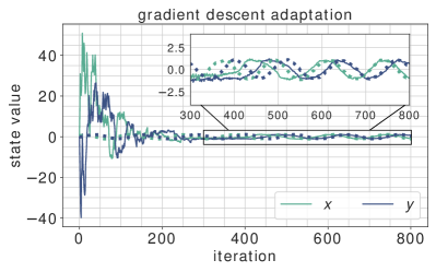
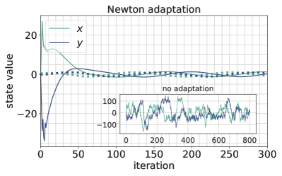
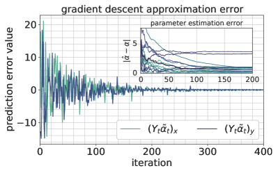
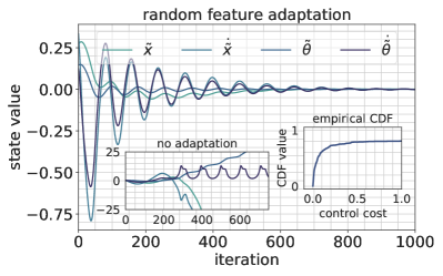
Figure 1: (Top left) Sample trajectory for online gradient descent (solid) and the comparator (dotted). Inset shows a close-up view near convergence. (Top right) Sample trajectory for online gradient descent (solid) and the comparator (dotted). Inset shows poor performance of the system without adaptation. (Bottom left) Prediction error for gradient descent (main figure) and parameter estimation error (inset). The parameters do not converge due to a lack of persistent excitation, but the prediction error still tends to zero. (Bottom right) LQR experiment with random features. Main figure shows the performance of one trajectory with adaptation. The right inset shows the empirical CDF of average control performance with random feature adaptation. The left inset shows divergent behavior of one trajectory without adaptation.

6.2 Online Convex Optimization Adaptation

To demonstrate the applicability of our OCO-inspired discrete-time adaptation laws, we study the following discrete-time nonlinear system

$$x_{t+1} =x_{t}+\tau\left(-y_{t}+\frac{x_{t}}{\sqrt{x_{t}^{2}+y_{t}^{2}}}-x_{t}+Y_{x}(x_{t},t)^{\mathsf{T}}\tilde{\alpha}_{t}\right)+\sqrt{\tau}\sigma w_{t,1}\>,$$ (6.1)

$$y_{t+1} =y_{t}+\tau\left(x_{t}+\frac{y_{t}}{\sqrt{x_{t}^{2}+y_{t}^{2}}}-y_{t}+Y_{y}(y_{t},t)^{\mathsf{T}}\tilde{\alpha}_{t}\right)+\sqrt{\tau}\sigma w_{t,2}$$

for $\tau=0.05$, $\sigma=0.1$, and $w_{t,i}\sim N(0,1)$. The nominal system for (6.1) is a forward-Euler discretization of the continuous-time system $\dot{x}=-y+\frac{x}{\sqrt{x^{2}+y^{2}}}-x$, $\dot{y}=x+\frac{y}{\sqrt{x^{2}+y^{2}}}-y$. In polar coordinates, the nominal system reads $\dot{r}=-(r-1)$, $\dot{\theta}=1$, which is contracting in the Euclidean metric towards the limit cycle $\dot{\theta}=1$ on the unit circle. This shows that the system in Euclidean coordinates is contracting in the radial direction in the metric $M(x,y)=\frac{\partial g}{\partial x}(x,y)^{\mathsf{T}}\frac{\partial g}{\partial x}(x,y)$, where $g$ is the nonlinear mapping $(x,y)\mapsto(r,\theta)$. The basis functions are taken to be $Y_{z}(z_{t},t)^{\mathsf{T}}=\sin(\omega(z_{t}+\sin(t)))$ where $z\in\{x,y\}$, the outer $\sin$ is taken element-wise, and $\omega\in\mathbb{R}^{p}$ is a vector of frequencies sampled uniformly between $0$ and $2\pi$. The estimated parameters $\hat{\alpha}_{t}$ are updated according to the OCO-inspired adaptive laws (3.7) or (3.8) analyzed in Section 5.2.

Results are shown in Figure 1. In the top-left pane, convergence of a sample trajectory towards the limit cycle is shown for gradient descent in solid, with the limit cycle itself plotted in dots. The inset displays a close-up view of convergence. In the top-right pane, convergence is shown for the online Newton method, which converges significantly faster and has a smoother trajectory than gradient descent. The inset displays a failure to converge without adaptation, demonstrating improved performance of the two adaptation algorithms in comparison to the system without adaptation. The bottom-left pane shows convergence of the two components of the prediction error $Y_{t}\tilde{\alpha}_{t}$ for gradient descent in the main figure, and shows parameter error trajectories in the inset. Note that the parameters do not converge to the true values due to a lack of persistent excitation.

7 Conclusion and Future Work

We present the first finite-time regret bounds for nonlinear adaptive control in discrete-time. Our work opens up many future directions of research. One direction is the possibility of logarithmic regret in our setting, given that it is achievable in various LQR problems (Agarwal et al., 2019b; Cassel et al., 2020; Foster and Simchowitz, 2020). A second question is handling state-dependent $Y(x,t)$ matrices in the $k$ timestep delay setting, or more broadly, studying the extended matching conditions of Kanellakopoulos et al. (1989); Krstić et al. (1995) for which timestep delays are a special case. Another direction concerns proving regret bounds for the velocity gradient algorithm in a stochastic setting. Furthermore, in the spirit of Agarwal et al. (2019a); Hazan et al. (2020), an extension of our analysis to handle more general cost functions and adversarial noise sequences would be quite impactful. Finally, understanding if sublinear regret guarantees are possible for a non-exponentially incrementally stable system would be interesting.

Appendix A Velocity Gradient Algorithms in Continuous-Time

In this section, we provide a brief introduction to the continuous-time formulation of velocity gradient algorithms, and show how the continuum limit of the online convex optimization-inspired algorithms from Section 3.1.2 can be seen as a particular case. A comprehensive treatment of velocity gradient algorithms in continuous-time can be found in Fradkov et al. (1999), Chapter 3.

In this section, we study the nonlinear dynamics with matched uncertainty

$$\dot{x}=f(x,t)+B(x,t)\left(u-Y(x,t)\alpha\right),$$ (A.1)

with $f(x,t)$ a known nominal dynamics satisfying $f(0,t)=0$ for all $t$, $B(x,t)$ and $Y(x,t)$ known matrix-valued functions, and $\alpha$ an unknown vector of parameters. As in the main text, we consider the certainty equivalence control input $u=Y(x,t)\hat{\alpha}$. We assume that $f(x,t)$, $B(x,t)$, and $Y(x,t)$ are continuous in $x$ and $t$.

The first result from Fradkov et al. (1999) we describe concerns the class of “local” velocity gradient algorithms, which use a Lyapunov function for the nominal system to adapt to unknown disturbances.

Theorem A.1.

Consider the system dynamics (A.1). Suppose $f(x,t)$ admits a twice continuously differentiable Lyapunov function $Q(x,t)$ satisfying for some positive $\rho,\mu$:

1. $Q(0,t)=0$ and $Q(x,t)\geqslant\mu\lVert x\rVert^{2}$ for all $x,t$.

2. For all $x,t$, $\langle\nabla_{x}Q(x,t),f(x,t)\rangle+\frac{\partial Q}{\partial t}(x,t)\leqslant-\rho Q(x,t)$.

Define

$$\omega(x,\hat{\alpha},t):=\langle\nabla_{x}Q(x,t),f(x,t)+B(x,t)Y(x,t)(\hat{\alpha}-\alpha)\rangle+\frac{\partial Q}{\partial t}(x,t)\>.$$

Then the adaptation law

$$\dot{\hat{\alpha}}=-\nabla_{\hat{\alpha}}\omega(x(t),\hat{\alpha}(t),t)$$ (A.2)

ensures that:

1. The solution $(x(t),\hat{\alpha}(t))$ exists and is unique for all $t\geqslant 0$.

2. The solution $(x(t),\hat{\alpha}(t))$ satisfies

   $$\int_{0}^{\infty}\lVert x(t)\rVert^{2}\>dt\leqslant\frac{1}{\rho\mu}\left(Q(x(0),0)+\frac{1}{2}\lVert\hat{\alpha}(0)-\alpha\rVert^{2}\right)\>.$$

3. The solution $(x(t),\hat{\alpha}(t))$ satisfies $x(t)\rightarrow 0$.

Proof.

By our continuity assumptions, we have that the closed-loop dynamics

$$\dot{x} =f(x,t)+B(x,t)Y(x,t)(\hat{\alpha}-\alpha)\>,$$

$$\dot{\hat{\alpha}} =-\nabla_{\hat{\alpha}}\omega(x,\hat{\alpha},t)\>,$$

is continuous in $t$ and locally Lipschitz in $(x,\alpha)$. Therefore, there exists a maximal interval $I(x(0),\hat{\alpha}(0))\subseteq\mathbb{R}_{\geqslant 0}$ for which the solution $(x(t),\hat{\alpha}(t))$ exists and is unique. Consider the Lyapunov-like function

$$V(x(t),\hat{\alpha}(t),t)=Q(x(t),t)+\frac{1}{2}\lVert\tilde{\alpha}(t)\rVert^{2}.$$

It is simple to show that $V$ has time derivative

$$\dot{V}(x(t),\hat{\alpha}(t),t)=\omega(x(t),\hat{\alpha}(t),t)-\langle\tilde{\alpha}(t),\nabla_{\hat{\alpha}}\omega(x(t),\hat{\alpha}(t),t)\rangle.$$

Hence,

$$\dot{V}(x(t),\hat{\alpha}(t),t)=\omega(x(t),\alpha,t)=\langle\nabla_{x}Q(x(t),t),f(x,t)\rangle+\frac{\partial Q}{\partial t}(x,t)\leqslant-\rho Q(x(t),t)\leqslant-\rho\mu\lVert x(t)\rVert^{2},$$

which shows that $x(t)$ and $\hat{\alpha}(t)$ remain uniformly bounded for all $t\in I(x(0),\hat{\alpha}(0))$. This in turn implies that the solution $(x(t),\hat{\alpha}(t))$ exists and is unique for all $t\geqslant 0$ (see e.g., Theorem 3.3 of Khalil (2002)).

Integrating both sides of the above differential inequality shows that

$$\int_{0}^{\infty}\lVert x(t)\rVert^{2}\>dt\leqslant\frac{1}{\rho\mu}\left(Q(x(0),0)+\frac{1}{2}\lVert\hat{\alpha}(0)-\alpha\rVert^{2}\right).$$

By the assumption that $f$, $B$, and $Y$ are continuous and that $Q$ is twice continuously differentiable, it is straightforward to check that $\sup_{t\geqslant 0}|\ddot{V}(x(t),\hat{\alpha}(t),t)|<\infty$. We have therefore shown that $\lim_{t\to\infty}V(x(t),\hat{\alpha}(t),t)$ exists and is finite, and also that $\dot{V}(x(t),\hat{\alpha}(t),t)$ is uniformly continuous in $t$. Applying Barbalat’s lemma (see e.g., Section 4.5.2 of Slotine and Li (1991)) yields the conclusion that $\lim_{t\to\infty}\dot{V}(x(t),\hat{\alpha}(t),t)=0$. But this implies that:

$$0=\lim_{t\to\infty}\dot{V}(x(t),\hat{\alpha}(t),t)\leqslant\limsup_{t\to\infty}\left[-\rho\mu\lVert x(t)\rVert^{2}\right]\leqslant 0\>.$$

Hence $x(t)\rightarrow 0$ as $t\rightarrow\infty$. ∎

In general, the proof of Theorem A.1 works as long as $\omega(x,\hat{\alpha},t)$ is convex in $\hat{\alpha}$. In this case, one has that the inequality $\dot{V}(x(t),\hat{\alpha}(t),t)\leqslant\omega(x(t),\alpha,t)$ holds.

The continuous-time formulation (A.2) gives justification for the name “velocity gradient”; $\omega(x(t),\hat{\alpha}(t),t)$ is the time derivative (velocity) of $Q(x(t),t)$ along the flow of the disturbed system. The adaptation algorithm is then derived by taking the gradient with respect to the parameters of this velocity. Moreover, (A.2) provides an explanation for the discrete-time requirement that $\nabla_{x}Q(x,t)$ be evaluated at $x_{t+1}$. In continuous-time, the instantaneous time derivative of $Q(x(t),t)$ provides information about the current function approximation error $B(x(t),t)Y(x(t),t)\tilde{\alpha}(t)$, which is only contained in $x_{t+1}$ in discrete-time.

A second class of “integral” velocity gradient algorithms from Fradkov et al. (1999) can be obtained under a different set of assumptions, as shown next. These algorithms proceed by updating the parameters along the gradient of an instantaneous loss function $R(x,\hat{\alpha},t)$. They then provide guarantees on the integral of $R(x,\hat{\alpha},t)$ along trajectories of the system. In general, such a guarantee does not imply boundedness of the state, which must be shown independently.

Theorem A.2.

Let $R(x,\hat{\alpha},t)$ denote a non-negative function that is convex in $\hat{\alpha}$ for all $x,t$. Let $\mu(t)$ denote a non-negative function such that $\int_{0}^{\infty}\mu(t)\>dt<\infty$ and $\lim_{t\rightarrow\infty}\mu(t)=0$. Assume there exists some vector of parameters $\alpha$ satisfying $R(x,\alpha,t)\leqslant\mu(t)$ for all $x,t$. Then the adaptation law

$$\dot{\hat{\alpha}}=-\nabla_{\hat{\alpha}}R(x(t),\hat{\alpha}(t),t)$$ (A.3)

ensures that

$$\int_{0}^{t}R(x(t^{\prime}),\hat{\alpha}(t^{\prime}),t^{\prime})\>dt^{\prime}\leqslant\frac{1}{2}\lVert\hat{\alpha}(0)-\alpha\rVert^{2}+\int_{0}^{\infty}\mu(t)\>dt.$$

for any $t\geqslant 0$ in the maximal interval of existence $I(x(0),\hat{\alpha}(0))$.

Proof.

Consider the Lyapunov-like function

$$V(x(t),\hat{\alpha}(t),t)=\int_{0}^{t}R(x(t^{\prime}),\hat{\alpha}(t^{\prime}),t^{\prime})\>dt^{\prime}+\frac{1}{2}\lVert\tilde{\alpha}(t)\rVert^{2}+\int_{t}^{\infty}\mu(t^{\prime})\>dt^{\prime}.$$

Note that $V(x(t),\hat{\alpha}(t),t)$ has its time derivative given by

$$\dot{V}(x(t),\hat{\alpha}(t),t)=R(x(t),\hat{\alpha}(t),t)-\langle\tilde{\alpha}(t),\nabla_{\hat{\alpha}}R(x(t),\hat{\alpha}(t),t)\rangle-\mu(t).$$

By convexity of $R(x,\hat{\alpha},t)$ in $\hat{\alpha}$, we have

$$\dot{V}(x(t),\hat{\alpha}(t),t)\leqslant R(x(t),\alpha,t)-\mu(t)\leqslant 0.$$

Because $\dot{V}(x(t),\hat{\alpha}(t),t)\leqslant 0$, and because each term in $V(x(t),\hat{\alpha}(t),t)$ is positive,

$$\int_{0}^{t}R(x(t^{\prime}),\hat{\alpha}(t^{\prime}),t^{\prime})\>dt^{\prime}\leqslant V(x(t),\hat{\alpha}(t),t)\leqslant V(x(0),\hat{\alpha}(0),0)=\frac{1}{2}\lVert\hat{\alpha}(0)-\alpha\rVert^{2}+\int_{0}^{\infty}\mu(t)\>dt.$$

∎

An important case for Theorem A.2 is when $R(x(t),\hat{\alpha}(t),t)$ is the squared prediction error, i.e.,

$$R(x,\hat{\alpha},t)=\frac{1}{2}\lVert B(x,t)Y(x,t)\tilde{\alpha}\rVert^{2}.$$ (A.4)

In this case, $R(x,\alpha,t)=0$, so that $\mu(t)$ can be taken to be zero. With the choice of $R$ given in (A.4), the resulting adaptation law (A.3) becomes the gradient flow dynamics

$$\dot{\hat{\alpha}}=-Y(x,t)^{\mathsf{T}}B(x,t)^{\mathsf{T}}B(x,t)Y(x,t)\tilde{\alpha}\>.$$ (A.5)

Furthermore, Theorem A.2 states that for any $t$ in the maximal interval of existence,

$$\int_{0}^{t}\lVert B(x(s),s)Y(x(s),s)\tilde{\alpha}(s)\rVert^{2}\>ds\leqslant\lVert\hat{\alpha}(0)-\alpha\rVert^{2}\>.$$

In this sense, the least-squares algorithms in Section 3.1.2 can be seen as an instance of the integral form of velocity gradient. Because we consider the deterministic setting here, we can state a stronger result: by Barbalat’s Lemma, this $O(1)$ guarantee on the prediction regret also implies that the function approximation error $B(x(t),t)Y(x(t),t)\tilde{\alpha}(t)\rightarrow 0$. Furthermore, the next proposition shows how to turn this $O(1)$ prediction regret bound into an $O(1)$ bound on the control regret.

Proposition A.3.

Suppose $f(x,t)$ admits a continuously differentiable Lyapunov function $Q(x,t)$ satisfying for some positive $\rho,\mu,L_{Q}$:

1. $Q(0,t)=0$ and $Q(x,t)\geqslant\mu\lVert x\rVert^{2}$ for all $x,t$.

2. $x\mapsto\nabla_{x}Q(x,t)$ is $L_{Q}$-Lipschitz for all $t$.

3. For all $x,t$, $\langle\nabla_{x}Q(x,t),f(x,t)\rangle+\frac{\partial Q}{\partial t}(x,t)\leqslant-\rho Q(x,t)$.

Let $u(x,\xi,t)$ and $g(x,\xi,t)$ be continuous functions, and consider the dynamics:

$$\dot{x}(t) =f(x,t)+u(x,\xi,t)\>,$$

$$\dot{\xi}(t) =g(x,\xi,t)\>.$$

For every $t\geqslant 0$ in the maximal interval of existence $I(x(0),\xi(0))$, we have:

$$\lVert x(t)\rVert\leqslant\sqrt{\frac{Q(x(0),0)}{\mu}+\frac{L_{Q}^{2}}{4\mu(1-\gamma)\rho}\int_{0}^{t}\lVert u(x(s),\xi(s),s)\rVert^{2}\>ds}\>.$$ (A.6)

Furthermore, for all $T\in I(x(0),\xi(0))$, we have:

$$\int_{0}^{T}\lVert x(t)\rVert^{2}\>dt\leqslant\frac{Q(x(0),0)}{\mu\gamma\rho}+\frac{L_{Q}^{2}}{4\mu^{2}(1-\gamma)\gamma\rho^{2}}\int_{0}^{T}\lVert u(x(t),\xi(t),t)\rVert^{2}\>dt\>.$$ (A.7)

Finally, suppose that for all $t\in I(x(0),\xi(0))$ the following inequality holds:

$$\int_{0}^{t}\lVert u(x(s),\xi(s),s)\rVert^{2}\>ds\leqslant B_{0}\>.$$

Then, the solution $(x(t),\xi(t))$ exists for all $t\geqslant 0$, and therefore:

$$\int_{0}^{\infty}\lVert x(t)\rVert^{2}\>dt\leqslant\frac{Q(x(0),0)}{\mu\gamma\rho}+\frac{L_{Q}^{2}B_{0}}{4\mu^{2}(1-\gamma)\gamma\rho^{2}}\>.$$ (A.8)

Proof.

Since zero is a global minimum of the map $x\mapsto Q(x,t)$ for all $t$, we have that $\nabla_{x}Q(0,t)=0$ for all $t$. Therefore, for any $\varepsilon>0$:

$$\frac{d}{dt}Q(x,t) =\langle\nabla_{x}Q(x,t),f(x,t)+u(x,t)\rangle+\frac{\partial Q}{\partial t}(x,t)$$

$$=\langle\nabla_{x}Q(x,t),f(x,t)\rangle+\frac{\partial Q}{\partial t}(x,t)+\langle\nabla_{x}Q(x,t),u(x,t)\rangle$$

$$\leqslant-\rho Q(x,t)+\lVert\nabla_{x}Q(x,t)\rVert\lVert u(x,t)\rVert$$

$$\leqslant-\rho Q(x,t)+L_{Q}\lVert x(t)\rVert\lVert u(x,t)\rVert$$

$$\leqslant-\rho Q(x,t)+\frac{\varepsilon L_{Q}^{2}}{2}\lVert x(t)\rVert^{2}+\frac{1}{2\varepsilon}\lVert u(x,t)\rVert^{2}$$

$$\leqslant-\gamma\rho Q(x,t)+\left[-(1-\gamma)\rho+\frac{\varepsilon L_{Q}^{2}}{2\mu}\right]Q(x,t)+\frac{1}{2\varepsilon}\lVert u(x,t)\rVert^{2}\>.$$

Setting $\varepsilon=2\mu(1-\gamma)\rho/L_{Q}^{2}$,

$$\frac{d}{dt}Q(x,t)\leqslant-\gamma\rho Q(x,t)+\frac{L_{Q}^{2}}{4\mu(1-\gamma)\rho}\lVert u(x,t)\rVert^{2}\>.$$

By the comparison lemma,

$$\mu\lVert x(t)\rVert^{2} \leqslant Q(x(t),t)\leqslant e^{-\gamma\rho t}Q(x(0),0)+\frac{L_{Q}^{2}}{4\mu(1-\gamma)\rho}\int_{0}^{t}e^{-\gamma\rho(t-s)}\lVert u(x(s),s)\rVert^{2}\>ds\>.$$

This establishes (A.6). Furthermore, integrating the above inequality from zero to $T$,

$$\int_{0}^{T}\lVert x(t)\rVert^{2}\>dt \leqslant\frac{Q(x(0),0)}{\mu}\int_{0}^{T}e^{-\gamma\rho t}\>dt+\frac{L_{Q}^{2}}{4\mu^{2}(1-\gamma)\rho}\int_{0}^{T}\int_{0}^{t}e^{-\gamma\rho(t-s)}\lVert u(x(s),s)\rVert^{2}\>ds\>dt$$

$$=\frac{Q(x(0),0)}{\mu}\int_{0}^{T}e^{-\gamma\rho t}\>dt+\frac{L_{Q}^{2}}{4\mu^{2}(1-\gamma)\rho}\int_{0}^{T}\left[\int_{0}^{T-t}e^{-\gamma\rho s}\>ds\right]\lVert u(x(t),t)\rVert^{2}\>dt$$

$$\leqslant\frac{Q(x(0),0)}{\mu\gamma\rho}+\frac{L_{Q}^{2}}{4\mu^{2}(1-\gamma)\gamma\rho^{2}}\int_{0}^{T}\lVert u(x(t),t)\rVert^{2}\>dt\>.$$

This establishes (A.7). The claim (A.8) follows from (A.6), (A.7), and Theorem 3.3 of Khalil (2002). ∎

We conclude this section by noting that (A.5) cannot be directly implemented due to the dependence on $\tilde{\alpha}(t)$. In discrete-time, this can be remedied as described in Section 3.1.2. In continuous-time, additional structural requirements are needed, which we briefly describe. Because the quantity $B(x(t),t)Y(x(t),t)\tilde{\alpha}(t)$ is contained in $\dot{x}$, the update (A.5) can be implemented through the proportional-integral construction (see e.g., Astolfi and Ortega (2003); Boffi and Slotine (2020))

$$\hat{\alpha}(t) =\bar{\alpha}(t)-Y^{\mathsf{T}}(x(t),t)B^{\mathsf{T}}(x(t),t)x(t)+\psi(x(t))\>,$$

$$\dot{\bar{\alpha}}(t) =Y^{\mathsf{T}}(x(t),t)B^{\mathsf{T}}(x(t),t)f(x(t),t)+\frac{\partial\left[Y^{\mathsf{T}}(x(t),t)B^{\mathsf{T}}(x(t),t)\right]}{\partial t}x(t)\>.$$

Here, $\psi(x)$ is a function that satisfies

$$\frac{\partial\psi(x)}{\partial x_{i}}=\frac{\partial\left[Y(x,t)^{\mathsf{T}}B(x,t)^{\mathsf{T}}\right]}{\partial x_{i}}x\>,$$

i.e., $\frac{\partial\left[Y(x,t)^{\mathsf{T}}B(x,t)^{\mathsf{T}}\right]}{\partial x_{i}}x$ must be the gradient of some auxiliary function $\psi(x)$. In general, this is a strong requirement that may not be satisfied by the system.

Appendix B Discrete-Time Stability of Zero-Order Hold Closed-Loop Systems

In this section, we study under what conditions the stability behavior of a continuous-time system is preserved under discrete sampling. In particular, we consider the following continuous-time system $f(x,u,t)$ with a continuous-time feedback law $\pi(x,t)$:

$$\dot{x}(t)=f(x(t),\pi(x(t),t),t)\>.$$

We are interested in understanding the effect of a discrete implementation for the control law $\pi$ via a zero-order hold at resolution $\tau$, specifically:

$$\dot{x}(t)=f(x(t),\pi(x(\lfloor t/\tau\rfloor\tau),\lfloor t/\tau\rfloor\tau),t)\>.$$

We will view this zero-order hold as inducing an associated discrete-time system. Let the flow map $\Phi(x,s,t)$ denote the solution $\xi(t)$ of the dynamics

$$\dot{\xi}(t)=f(\xi(t),\pi(x,s),t)\>,\>\>\xi(s)=x\>.$$

For simplicity, we assume in this section that the solution $\Phi(x,s,t)$ exists and is unique. The closed-loop discrete-time system we consider is

$$x_{t+1}=g(x_{t},t):=\Phi(x_{t},\tau t,\tau(t+1))\>.$$

We address two specific questions. First, if $Q(x,t)$ is a Lyapunov function for $f(x,\pi(x,t),t)$, when does $(x,t)\mapsto Q(x,\tau t)$ remain a discrete-time Lyapunov function for $g(x,t)$? Similarly, if $M(x,t)$ is a contraction metric for $f(x,\pi(x,t),t)$, when does $(x,t)\mapsto M(x,\tau t)$ remain a discrete-time contraction metric for $g(x,t)$? To do so, we will derive upper bounds on the sampling rate to ensure preservation of these stability properties. For simplicity, we perform our analysis at fixed resolution, but irregularly sampled time points may also be used so long as they satisfy our restrictions.

Before we begin our analysis, we start with a regularity assumption on both the dynamics $f$ and the policy $\pi$.

Definition B.1.

Let $f(x,u,t)$ and $\pi(x,t)$ be a dynamics and a policy. We say that $(f,\pi)$ is $(L_{f},L_{\pi})$-regular if $f\in C^{2}$, $\pi\in C^{0}$, and the following conditions hold:

1. $f(0,0,t)=0$  for all $t$.

2. $\pi(0,t)=0$  for all $t$.

3. $\max\left\{\left\lVert\frac{\partial f}{\partial x}(x,u,t)\right\rVert,\left\lVert\frac{\partial f}{\partial u}(x,u,t)\right\rVert,\left\lVert\frac{\partial^{2}f}{\partial x\partial t}(x,u,t)\right\rVert,\left\lVert\frac{\partial^{2}f}{\partial u\partial t}(x,u,t)\right\rVert,\left\lVert\frac{\partial^{2}f}{\partial x^{2}}(x,u,t)\right\rVert\right\}\leqslant L_{f}$ for all $x,u,t$.

4. $\left\lVert\frac{\partial\pi}{\partial x}(x,t)\right\rVert\leqslant L_{\pi}$ for all $x,t$.

Our first proposition bounds how far the solution $\Phi(x,s,s+\tau)$ deviates from the initial condition $x$ over a time period $\tau$. Roughly speaking, the proposition states that the deviation is a constant factor of $\lVert x\rVert$ as long as $\tau$ is on the order of $1/L_{f}$. Note that for notational simplicity a common bound $L_{f}$ is used Definition B.1, although our results extends immediately to finer individual bounds.

Proposition B.2.

Let $(f,\pi)$ be $(L_{f},L_{\pi})$-regular. Let the flow map $\Phi(x,s,t)$ denote the solution $\xi(t)$ of the dynamics

$$\dot{\xi}(t)=f(\xi(t),\pi(x,s),t)\>,\>\>\xi(s)=x\>.$$

We have that for any $\tau>0$:

$$\lVert\Phi(x,s,s+\tau)-x\rVert\leqslant(1+3L_{\pi})(e^{L_{f}\tau}-1)\lVert x\rVert\>.$$

As a consequence, we have:

$$\lVert\Phi(x,s,s+\tau)\rVert\leqslant(e^{L_{f}\tau}+3L_{\pi}(e^{L_{f}\tau}-1))\lVert x\rVert\leqslant(1+3L_{\pi})e^{L_{f}\tau}\lVert x\rVert\>.$$

Proof.

The proof follows by a direct application of the comparison lemma. We use the Lipschitz properties of both $f$ and $\pi$, which are implied by the regularity assumptions, to establish the necessary differential inequality. Let $v(t):=\lVert\xi(t)-x\rVert$. We note for any signal $z(t)$, we have $\frac{d}{dt}\lVert z(t)\rVert\leqslant\lVert\dot{z}\rVert$. Therefore, setting $\xi=\xi(t)$ to simplify the notation:

$$\frac{d}{dt}v(t) \leqslant\lVert\dot{\xi}(t)\rVert$$

$$=\lVert f(\xi,\pi(x,s),t)\rVert$$

$$=\lVert f(\xi,\pi(x,s),t)-f(x,\pi(x,t),t)+f(x,\pi(x,t),t)-f(0,0,t)\rVert$$

$$\leqslant\lVert f(\xi,\pi(x,s),t)-f(x,\pi(x,t),t)\rVert+\lVert f(x,\pi(x,t),t)-f(0,0,t)\rVert$$

$$=:T_{1}+T_{2}\>.$$

Next,

$$T_{1} =\lVert f(\xi,\pi(x,s),t)-f(x,\pi(x,t),t)\rVert$$

$$=\lVert f(\xi,\pi(x,s),t)-f(x,\pi(x,s),t)+f(x,\pi(x,s),t)-f(x,\pi(x,t),t)\rVert$$

$$\leqslant L_{f}\lVert\xi-x\rVert+L_{f}\lVert\pi(x,s)-\pi(x,t)\rVert$$

$$=L_{f}\lVert\xi-x\rVert+L_{f}\lVert\pi(x,s)-\pi(0,s)+\pi(0,t)-\pi(x,t)\rVert$$

$$\leqslant L_{f}\lVert\xi-x\rVert+2L_{f}L_{\pi}\lVert x\rVert\>.$$

Also,

$$T_{2} =\lVert f(x,\pi(x,t),t)-f(0,0,t)\rVert$$

$$=\lVert f(x,\pi(x,t),t)-f(0,\pi(x,t),t)+f(0,\pi(x,t),t)-f(0,0,t)\rVert$$

$$\leqslant L_{f}\lVert x\rVert+L_{f}\lVert\pi(x,t)\rVert$$

$$=L_{f}\lVert x\rVert+L_{f}\lVert\pi(x,t)-\pi(0,t)\rVert$$

$$\leqslant L_{f}(1+L_{\pi})\lVert x\rVert\>.$$

Therefore we have the following differential inequality:

$$\frac{d}{dt}v(t)\leqslant L_{f}v(t)+L_{f}(1+3L_{\pi})\lVert x\rVert\>.$$

The claim now follows by the comparison lemma. ∎

The next proposition shows that the error of the forward Euler approximation of the flow map $\Phi(x,s,s+\tau)$ and also its derivative $\frac{\partial\Phi}{\partial x}(x,s,s+\tau)$ scales as $O(\tau^{2})$.

Proposition B.3.

Let $(f,\pi)$ be $(L_{f},L_{\pi})$-regular, with $\min\{L_{f},L_{\pi}\}\geqslant 1$. Let $\Phi(x,s,t)$ be the solution $\xi(t)$ for the dynamics

$$\dot{\xi}(t)=f(\xi(t),\pi(x,s),t)\>,\>\>\xi(s)=x\>.$$

Fix any $\tau>0$. We have that:

$$\lVert\Phi(x,s,s+\tau)-(x+\tau f(x,\pi(x,s),s))\rVert\leqslant 5\tau^{2}L_{f}^{2}L_{\pi}e^{L_{f}\tau}\lVert x\rVert\>.$$ (B.1)

We also have:

$$\left\lVert\frac{\partial\Phi}{\partial x}(x,s,s+\tau)-\left(I+\tau\frac{\partial f}{\partial x}(x,\pi(x,s),s)\right)\right\rVert\leqslant\frac{7\tau^{2}}{2}L_{f}^{2}L_{\pi}e^{2L_{f}\tau}\max\{1,\lVert x\rVert\}\>.$$ (B.2)

Proof.

We first differentiate $\Phi(x,s,t)$ w.r.t. $t$ twice:

$$\frac{\partial\Phi}{\partial t}(x,s,t) =f(\xi(t),\pi(x,s),t)\>,$$

$$\frac{\partial^{2}\Phi}{\partial t^{2}}(x,s,t) =\frac{df}{dt}(\xi(t),\pi(x,s),t)=\frac{\partial f}{\partial x}(\xi(t),\pi(x,s),t)f(\xi(t),\pi(x,s),t)+\frac{\partial f}{\partial t}(\xi(t),\pi(x,s),t)\>.$$

By Taylor’s theorem, there exists some $\iota\in[s,s+\tau]$ such that:

$$\Phi(x,s,s+\tau)=\Phi(x,s,s)+\frac{\partial\Phi}{\partial t}(x,s,s)\tau+\frac{\tau^{2}}{2}\frac{\partial^{2}\Phi}{\partial t^{2}}(x,s,\iota)$$

$$=x+\tau f(x,\pi(x,s),s)+\frac{\tau^{2}}{2}\left(\frac{\partial f}{\partial x}(\xi(\iota),\pi(x,s),\iota)f(\xi(\iota),\pi(x,s),\iota)+\frac{\partial f}{\partial t}(\xi(\iota),\pi(x,s),\iota)\right)\>.$$

In order to bound the error term above, we make a few intermediate calculations. We use Proposition B.2 to bound:

$$\lVert f(\xi(\iota),\pi(x,s),\iota)\rVert =\lVert f(\xi(\iota),\pi(x,s),\iota)-f(0,\pi(x,s),\iota)+f(0,\pi(x,s),\iota)-f(0,0,\iota)\rVert$$

$$\leqslant L_{f}\lVert\xi(\iota)\rVert+L_{f}\lVert\pi(x,s)\rVert$$

$$=L_{f}\lVert\xi(\iota)\rVert+L_{f}\lVert\pi(x,s)-\pi(0,s)\rVert$$

$$\leqslant L_{f}\lVert\xi(\iota)\rVert+L_{f}L_{\pi}\lVert x\rVert$$

$$\leqslant L_{f}(1+3L_{\pi})e^{L_{f}\tau}\lVert x\rVert+L_{f}L_{\pi}\lVert x\rVert$$

$$\leqslant L_{f}(1+4L_{\pi})e^{L_{f}\tau}\lVert x\rVert$$

$$\leqslant 5L_{f}L_{\pi}e^{L_{f}\tau}\lVert x\rVert\>.$$

Again we use Proposition B.2, along with the fact that $\frac{\partial f}{\partial t}(0,0,t)=0$ for all $t$ due to the regularity assumptions on $f$, to bound:

$$\left\lVert\frac{\partial f}{\partial t}(\xi(\iota),\pi(x,s),\iota)\right\rVert =\left\lVert\frac{\partial f}{\partial t}(\xi(\iota),\pi(x,s),\iota)-\frac{\partial f}{\partial t}(0,\pi(x,s),\iota)+\frac{\partial f}{\partial t}(0,\pi(x,s),\iota)-\frac{\partial f}{\partial t}(0,0,\iota)\right\rVert$$

$$\leqslant L_{f}\lVert\xi(\iota)\rVert+L_{f}\lVert\pi(x,s)\rVert$$

$$\leqslant L_{f}\lVert\xi(\iota)\rVert+L_{f}L_{\pi}\lVert x\rVert$$

$$\leqslant 5L_{f}L_{\pi}e^{L_{f}\tau}\lVert x\rVert\>.$$

Therefore:

$$\lVert\Phi(x,s,s+\tau)-(x+\tau f(x,\pi(x,s),s))\rVert$$

$$\leqslant\left\lVert\frac{\tau^{2}}{2}\left(\frac{\partial f}{\partial x}(\xi(\iota),\pi(x,s),\iota)f(\xi(\iota),\pi(x,s),\iota)+\frac{\partial f}{\partial t}(\xi(\iota),\pi(x,s),\iota)\right)\right\rVert$$

$$\leqslant 5\tau^{2}L_{f}^{2}L_{\pi}e^{L_{f}\tau}\lVert x\rVert\>.$$

This establishes (B.1).

Next, let $\Psi(x,s,t)$ be the solution $\Xi(t)$ for the matrix-valued dynamics:

$$\dot{\Xi}(t)=\frac{\partial f}{\partial x}(\xi(t),\pi(x,s),t)\Xi(t)\>,\>\>\Xi(s)=I\>.$$

A standard result in the theory of ordinary differential equations states that $\frac{\partial\Phi}{\partial x}(x,s,t)=\Psi(x,s,t)$. We can bound the norm $\lVert\Psi(x,s,t)\rVert$ as follows:

$$\lVert\Psi(x,s,t)\rVert =\left\lVert\exp\left(\int_{s}^{t}\frac{\partial f}{\partial x}(\xi(\tau),\pi(x,s),\tau)\>d\tau\right)\right\rVert$$

$$\leqslant\exp\left(\int_{s}^{t}\left\lVert\frac{\partial f}{\partial x}(\xi(\tau),\pi(x,s),\tau)\right\rVert\>d\tau\right)\leqslant\exp(L_{f}(t-s))\>.$$

Furthermore, differentiating $\Psi$ w.r.t. $t$ twice:

$$\frac{\partial\Psi}{\partial t}(x,s,t) =\frac{\partial f}{\partial x}(\xi(t),\pi(x,s),t)\Xi(t)\>,$$

$$\frac{\partial^{2}\Psi}{\partial t^{2}}(x,s,t) =\frac{d}{dt}\left(\frac{\partial f}{\partial x}(\xi(t),\pi(x,s),t)\Xi(t)\right)$$

$$=\frac{\partial f}{\partial x}(\xi(t),\pi(x,s),t)\frac{\partial f}{\partial x}(\xi(t),\pi(x,s),t)\Xi(t)$$

$$\qquad+\left(\frac{\partial^{2}f}{\partial x^{2}}(\xi(t),\pi(x,s),t)f(\xi(t),\pi(x,s),t)+\frac{\partial^{2}f}{\partial t\partial x}(\xi(t),\pi(x,s),t)\right)\Xi(t)\>.$$

By Taylor’s theorem, there exists an $\iota\in[s,s+\tau]$ such that:

$$\Psi(x,s,s+\tau) =\Psi(x,s,s)+\tau\frac{\partial\Psi}{\partial t}(x,s,s)+\frac{\tau^{2}}{2}\frac{\partial^{2}\Psi}{\partial t^{2}}(x,s,\iota)$$

$$=I+\tau\frac{\partial f}{\partial x}(x,\pi(x,s),s)+\frac{\tau^{2}}{2}\frac{\partial^{2}\Psi}{\partial t^{2}}(x,s,\iota)\>.$$

Using the estimate on $\lVert\Psi(x,s,t)\rVert$ above, we bound:

$$\left\lVert\frac{\partial f}{\partial x}(\xi(\iota),\pi(x,s),\iota)\frac{\partial f}{\partial x}(\xi(\iota),\pi(x,s),\iota)\Xi(\iota)\right\rVert\leqslant L_{f}^{2}e^{L_{f}\tau}\>.$$

Furthermore by the estimates on $\lVert\Psi(x,s,t)\rVert$ and $\lVert f(\xi(t),\pi(x,s),t)\rVert$,

$$\left\lVert\left(\frac{\partial^{2}f}{\partial x^{2}}(\xi(\iota),\pi(x,s),\iota)f(\xi(\iota),\pi(x,s),\iota)+\frac{\partial^{2}f}{\partial t\partial x}(\xi(\iota),\pi(x,s),\iota)\right)\Xi(\iota)\right\rVert$$

$$\leqslant L_{f}(1+\lVert f(\xi(\iota),\pi(x,s),\iota)\rVert)e^{L_{f}\tau}$$

$$\leqslant L_{f}(1+5L_{f}L_{\pi}e^{L_{f}\tau}\lVert x\rVert)e^{L_{f}\tau}$$

$$\leqslant 6L_{f}^{2}L_{\pi}e^{2L_{f}\tau}\max\{1,\lVert x\rVert\}\>.$$

Therefore:

$$\left\lVert\Psi(x,s,s+\tau)-\left(I+\tau\frac{\partial f}{\partial x}(x,\pi(x,s),s)\right)\right\rVert \leqslant\left\lVert\frac{\tau^{2}}{2}\frac{\partial^{2}\Psi}{\partial t^{2}}(x,s,\iota)\right\rVert$$

$$\leqslant\frac{\tau^{2}}{2}\left[L_{f}^{2}e^{L_{f}\tau}+6L_{f}^{2}L_{\pi}e^{2L_{f}\tau}\max\{1,\lVert x\rVert\}\right]$$

$$\leqslant\frac{7\tau^{2}}{2}L_{f}^{2}L_{\pi}e^{2L_{f}\tau}\max\{1,\lVert x\rVert\}\>.$$

This establishes (B.2). ∎

Our first main result gives conditions on $\tau$ for which Lyapunov stability is preserved with zero-order holds.

Theorem B.4.

Let $(f,\pi)$ be $(L_{f},L_{\pi})$-regular, with $\min\{L_{f},L_{\pi}\}\geqslant 1$. Let $\Phi(x,s,t)$ be the solution $\xi(t)$ for the dynamics

$$\dot{\xi}(t)=f(\xi(t),\pi(x,s),t)\>,\>\>\xi(s)=x\>.$$

Let $Q(x,t)\in C^{2}$ be a Lyapunov function that satisfies, for positive $\mu,\rho$ and $L_{Q}\geqslant 1$, the conditions:

1. $Q(0,t)=0$ for all $t$.

2. $Q(x,t)\geqslant\mu\lVert x\rVert^{2}$ for all $x,t$.

3. $\langle\nabla_{x}Q(x,t),f(x,\pi(x,t),t)\rangle+\frac{\partial Q}{\partial t}(x,t)\leqslant-\rho Q(x,t)$ for all $x,t$.

4. $\left\lVert\frac{\partial^{2}Q}{\partial x^{2}}(x,t)\right\rVert\leqslant L_{Q}$ for all $x,t$.

5. $\left\lVert\frac{\partial^{2}Q}{\partial t\partial x}(x,t)-\frac{\partial^{2}Q}{\partial t\partial x}(y,t)\right\rVert\leqslant L_{Q}\lVert x-y\rVert$ for all $x,y,t$.

6. $\left|\frac{\partial^{2}Q}{\partial t^{2}}(x,t)\right|\leqslant L_{Q}\lVert x\rVert^{2}$ for all $x,t$.

Fix a $\gamma\in(0,1)$ and $\tau>0$. Define the discrete-time system $g(x,t):=\Phi(x,\tau t,\tau(t+1))$. As long as $\tau$ satisfies:

$$\tau\leqslant\min\left\{\frac{1}{L_{f}},\frac{1}{\gamma\rho},\frac{2(1-\gamma)\rho\mu}{895L_{Q}L_{f}^{2}L_{\pi}^{2}}\right\}\>,$$

then the function $V(x,t):=Q(x,\tau t)$ is a valid Lyapunov function for $g(x,t)$ with rate $(1-\gamma\tau\rho)$, i.e., for all $x,t$:

$$V(g(x,t),t+1)\leqslant(1-\gamma\tau\rho)V(x,t)\>.$$ (B.3)

Proof.

We define the function $h(t):=Q(\Phi(x,s,t),t)$. Differentiating $h$ twice,

$$\frac{\partial h}{\partial t}(t) =\frac{\partial Q}{\partial x}(\Phi(x,s,t),t)f(\xi(t),\pi(x,s),t)+\frac{\partial Q}{\partial t}(\Phi(x,s,t),t)\>,$$

$$\frac{\partial^{2}h}{\partial t^{2}}(t) =\frac{\partial Q}{\partial x}(\Phi(x,s,t),t)\left(\frac{\partial f}{\partial x}(\xi(t),\pi(x,s),t)f(\xi(t),\pi(x,s),t)+\frac{\partial f}{\partial t}(\xi(t),\pi(x,s),t)\right)$$

$$\qquad+\left(\frac{\partial^{2}Q}{\partial x^{2}}(\Phi(x,s,t),t)f(\xi(t),\pi(x,s),t)+\frac{\partial^{2}Q}{\partial t\partial x}(\Phi(x,s,t),t)\right)f(\xi(t),\pi(x,s),t)$$

$$\qquad+\frac{\partial^{2}Q}{\partial x\partial t}(\Phi(x,s,t),t)f(\xi(t),\pi(x,s),t)+\frac{\partial^{2}Q}{\partial t^{2}}(\Phi(x,s,t),t)\>.$$

By Taylor’s theorem, there exists an $\iota\in[s,s+\tau]$ such that:

$$h(s+\tau) =h(s)+\tau\frac{\partial h}{\partial t}(s)+\frac{\tau^{2}}{2}\frac{\partial^{2}h}{\partial t^{2}}(\iota)$$

$$=Q(x,s)+\tau\left[\langle\nabla_{x}Q(x,s),f(x,\pi(x,s),s)\rangle+\frac{\partial Q}{\partial t}(x,s)\right]+\frac{\tau^{2}}{2}\frac{\partial^{2}h}{\partial t^{2}}(\iota)$$

$$\leqslant Q(x,s)-\tau\rho Q(x,s)+\frac{\tau^{2}}{2}\frac{\partial^{2}h}{\partial t^{2}}(\iota)$$

$$=(1-\tau\rho\gamma)Q(x,s)-\tau\rho(1-\gamma)Q(x,s)+\frac{\tau^{2}}{2}\frac{\partial^{2}h}{\partial t^{2}}(\iota)$$

$$\leqslant(1-\tau\rho\gamma)Q(x,s)-\tau\rho(1-\gamma)\mu\lVert x\rVert^{2}+\frac{\tau^{2}}{2}\frac{\partial^{2}h}{\partial t^{2}}(\iota)\>.$$ (B.4)

Above, the first inequality follows from the continuous-time Lyapunov condition. The remainder of the proof focuses on estimating a bound for $\left|\frac{\partial^{2}h}{\partial t^{2}}(t)\right|$. First, we collect a few useful facts. Since zero is a global minimum of $x\mapsto Q(x,t)$ for every $t$, we have that $\frac{\partial Q}{\partial x}(0,t)=0$ for every $t$. Therefore:

$$\left\lVert\frac{\partial Q}{\partial x}(\xi(\iota),\iota)\right\rVert =\left\lVert\frac{\partial Q}{\partial x}(\xi(\iota),\iota)-\frac{\partial Q}{\partial x}(0,\iota)\right\rVert\leqslant L_{Q}\lVert\xi(\iota)\rVert$$

$$\leqslant L_{Q}(1+3L_{\pi})e^{L_{f}\tau}\lVert x\rVert\leqslant 4L_{Q}L_{\pi}e^{L_{f}\tau}\lVert x\rVert\>.$$

Above, the second to last inequality follows from Proposition B.2. Next, the proof of Proposition B.3 derives the following estimates:

$$\max\left\{\lVert f(\xi(\iota),\pi(x,s),\iota)\rVert,\left\lVert\frac{\partial f}{\partial t}(\xi(t),\pi(x,s),t)\right\rVert\right\}\leqslant 5L_{f}L_{\pi}e^{L_{f}\tau}\lVert x\rVert\>.$$

Using these estimates, we can bound:

$$\left|\frac{\partial Q}{\partial x}(\xi(\iota),\iota)\left(\frac{\partial f}{\partial x}(\xi(\iota),\pi(x,s),\iota)f(\xi(\iota),\pi(x,s),\iota)+\frac{\partial f}{\partial t}(\xi(\iota),\pi(x,s),\iota)\right)\right|$$

$$\leqslant 4L_{Q}L_{\pi}e^{L_{f}\tau}\lVert x\rVert\cdot\left[5L_{f}^{2}L_{\pi}e^{L_{f}\tau}\lVert x\rVert+5L_{f}L_{\pi}e^{L_{f}\tau}\lVert x\rVert\right]$$

$$\leqslant 40L_{Q}L_{f}^{2}L_{\pi}^{2}e^{2L_{f}\tau}\lVert x\rVert^{2}\>.$$

Next, we observe that $\frac{\partial^{2}Q}{\partial t\partial x}(0,t)=0$ for all $t$, which allows us to bound:

$$\left|\left(\frac{\partial^{2}Q}{\partial x^{2}}(\xi(\iota),\iota)f(\xi(\iota),\pi(x,s),\iota)+\frac{\partial^{2}Q}{\partial t\partial x}(\xi(\iota),\iota)\right)f(\xi(\iota),\pi(x,s),\iota)\right|$$

$$\leqslant L_{Q}\lVert f(\xi(\iota),\pi(x,s),\iota)\rVert^{2}+\left\lVert\frac{\partial^{2}Q}{\partial t\partial x}(\xi(\iota),\iota)\right\rVert\lVert f(\xi(\iota),\pi(x,s),\iota)\rVert$$

$$\leqslant L_{Q}\lVert f(\xi(\iota),\pi(x,s),\iota)\rVert^{2}+L_{Q}\lVert\xi(\iota)\rVert\lVert f(\xi(\iota),\pi(x,s),\iota)\rVert$$

$$\leqslant 25L_{Q}L_{f}^{2}L_{\pi}^{2}e^{2L_{f}\tau}\lVert x\rVert^{2}+L_{Q}(1+3L_{\pi})e^{L_{f}\tau}\lVert x\rVert\cdot 5L_{f}L_{\pi}e^{L_{f}\tau}\lVert x\rVert$$

$$\leqslant 45L_{Q}L_{f}^{2}L_{\pi}^{2}e^{2L_{f}\tau}\lVert x\rVert^{2}\>.$$

Finally, we bound:

$$\left|\frac{\partial^{2}Q}{\partial x\partial t}(\xi(\iota),\iota)f(\xi(\iota),\pi(x,s),\iota)+\frac{\partial^{2}Q}{\partial t^{2}}(\xi(\iota),\iota)\right|$$

$$\leqslant\left\lVert\frac{\partial^{2}Q}{\partial x\partial t}(\xi(\iota),\iota)\right\rVert\lVert f(\xi(\iota),\pi(x,s),\iota)\rVert+L_{Q}\lVert\xi(\iota)\rVert^{2}$$

$$\leqslant L_{Q}\lVert\xi(\iota)\rVert\lVert f(\xi(\iota),\pi(x,s),\iota)\rVert+L_{Q}\lVert\xi(\iota)\rVert^{2}$$

$$\leqslant L_{Q}(1+3L_{\pi})e^{L_{f}\tau}\lVert x\rVert\cdot 5L_{f}L_{\pi}e^{L_{f}\tau}\lVert x\rVert+L_{Q}(1+3L_{\pi})^{2}e^{2L_{f}\tau}\lVert x\rVert^{2}$$

$$\leqslant 36L_{Q}L_{f}L_{\pi}^{2}e^{2L_{f}\tau}\lVert x\rVert^{2}\>.$$

Combining these estimates:

$$\left|\frac{\partial^{2}h}{\partial t^{2}}(\iota)\right| \leqslant 40L_{Q}L_{f}^{2}L_{\pi}^{2}e^{2L_{f}\tau}\lVert x\rVert^{2}+45L_{Q}L_{f}^{2}L_{\pi}^{2}e^{2L_{f}\tau}\lVert x\rVert^{2}+36L_{Q}L_{f}L_{\pi}^{2}e^{2L_{f}\tau}\lVert x\rVert^{2}$$

$$\leqslant 121L_{Q}L_{f}^{2}L_{\pi}^{2}e^{2L_{f}\tau}\lVert x\rVert^{2}\leqslant 121e^{2}L_{Q}L_{f}^{2}L_{\pi}^{2}\lVert x\rVert^{2}\>,$$

where the last inequality follows since we assume $\tau\leqslant 1/L_{f}$. Continuing from (B.4),

$$h(s+\tau) \leqslant(1-\tau\rho\gamma)Q(x,s)-\tau\rho(1-\gamma)\mu\lVert x\rVert^{2}+\frac{\tau^{2}}{2}\frac{\partial^{2}h}{\partial t^{2}}(\iota)$$

$$\leqslant(1-\tau\rho\gamma)Q(x,s)-\tau\rho(1-\gamma)\mu\lVert x\rVert^{2}+\tau^{2}\frac{121}{2}e^{2}L_{Q}L_{f}^{2}L_{\pi}^{2}\lVert x\rVert^{2}$$

$$=(1-\tau\rho\gamma)Q(x,s)+\left[-\rho(1-\gamma)\mu+\tau\frac{121}{2}e^{2}L_{Q}L_{f}^{2}L_{\pi}^{2}\right]\tau\lVert x\rVert^{2}\>.$$

Hence as long as

$$-\rho(1-\gamma)\mu+\tau\frac{121}{2}e^{2}L_{Q}L_{f}^{2}L_{\pi}^{2}\leqslant 0\>,$$

then (B.3) holds. It is straightforward to check that the following condition suffices:

$$\tau\leqslant\frac{2\rho(1-\gamma)\mu}{895L_{Q}L_{f}^{2}L_{\pi}^{2}}\>.$$

The claim now follows. ∎

Before we proceed, we briefly describe the condition $\left|\frac{\partial^{2}Q}{\partial t^{2}}(x,t)\right|\leqslant L_{Q}\lVert x\rVert^{2}$ in Theorem B.4. Let us suppose that $Q\in C^{4}$, and define the function $\psi(x,t):=\frac{\partial^{2}Q}{\partial t^{2}}(x,t)$. By Taylor’s theorem, there exists a $\tilde{x}$ satisfying $\lVert\tilde{x}\rVert\leqslant\lVert x\rVert$ such that:

$$\psi(x,t)=\psi(0,t)+\frac{\partial\psi}{\partial x}(0,t)x+\frac{1}{2}x^{\mathsf{T}}\frac{\partial^{2}\psi}{\partial x^{2}}(\tilde{x},t)x\>.$$

First, since $Q(0,t)=0$ for all $t$, we know that $\frac{\partial Q}{\partial t}(0,t)=0$ for all $t$. Repeating this argument yields that $\frac{\partial^{2}Q}{\partial t^{2}}(0,t)=0$ for all $t$. Next, we know that $\frac{\partial Q}{\partial x}(0,t)=0$ for all $t$ because $x=0$ is a global minima of the function $x\mapsto Q(x,t)$ for all $t$. This means that $\frac{\partial^{2}Q}{\partial t\partial x}(0,t)=0$ for all $t$. Repeating this argument yields $\frac{\partial^{3}Q}{\partial t^{2}\partial x}(0,t)=0$ for all $t$. Swapping the order of differentiation yields that $\psi(0,t)=\frac{\partial}{\partial x}\frac{\partial^{2}Q}{\partial t^{2}}(0,t)=\frac{\partial^{3}Q}{\partial t^{2}\partial x}(0,t)=0$. Hence:

$$\left|\psi(x,t)\right|\leqslant\frac{1}{2}\left\lVert\frac{\partial^{2}\psi}{\partial x^{2}}(\tilde{x},t)\right\rVert\lVert x\rVert^{2}\>.$$

Therefore if $\frac{\partial^{2}\psi}{\partial x^{2}}$ is uniformly bounded, then this condition holds.

Our next main result gives conditions on $\tau$ for which contraction is preserved with zero-order holds.

Theorem B.5.

Let $(f,\pi)$ be $(L_{f},L_{\pi})$-regular, with $\min\{L_{f},L_{\pi}\}\geqslant 1$. Let $\Phi(x,s,t)$ be the solution $\xi(t)$ for the dynamics

$$\dot{\xi}(t)=f(\xi(t),\pi(x,s),t)\>,\>\>\xi(s)=x\>.$$

Let $M(x,t)\in C^{2}$ be a positive definite metric that satisfies, for positive $\mu,\lambda$ and $\min\{L,L_{M}\}\geqslant 1$, the conditions:

1. $\mu I\preccurlyeq M(x,t)\preccurlyeq LI$ for all $x,t$.

2. $\frac{\partial f}{\partial x}(x,\pi(x,t),t)^{\mathsf{T}}M(x,t)+M(x,t)\frac{\partial f}{\partial x}(x,\pi(x,t),t)+\dot{M}(x,t)\preccurlyeq-2\lambda M(x,t)$ for all $x,t$.

3. $\max\left\{\left\lVert\frac{\partial M}{\partial x}(x,t)\right\rVert,\left\lVert\frac{\partial M}{\partial t}(x,t)\right\rVert,\left\lVert\frac{\partial^{2}M}{\partial^{2}x}(x,t)\right\rVert,\left\lVert\frac{\partial^{2}M}{\partial x\partial t}(x,t)\right\rVert,\left\lVert\frac{\partial^{2}M}{\partial t^{2}}(x,t)\right\rVert\right\}\leqslant L_{M}$ for all $x,t$.

Pick a $\gamma\in(0,1)$, $\tau>0$, and $D\geqslant 1$. Define the discrete system $g(x,t):=\Phi(x,\tau t,\tau(t+1))$. As long as $\tau$ satisfies:

$$\tau\leqslant\min\left\{\frac{1}{L_{f}},\frac{1}{2\lambda\gamma},\frac{2\lambda(1-\gamma)\mu}{1463D^{2}LL_{M}L_{f}^{2}L_{\pi}^{2}}\right\}\>,$$

then for any $x$ satisfying $\lVert x\rVert\leqslant D$ and for any $t$, we have that $g(x,t)$ is contracting in the metric $V(x,t):=M(x,\tau t)$ with rate $(1-2\lambda\gamma\tau)$, i.e.,

$$\frac{\partial g}{\partial x}(x,t)^{\mathsf{T}}V(g(x,t),t+1)\frac{\partial g}{\partial x}(x,t)\preccurlyeq(1-2\lambda\gamma\tau)V(x,t)\>.$$ (B.5)

Proof.

We fix an $x$ satisfying $\lVert x\rVert\leqslant D$. Let $\Delta(x,s,\tau):=\frac{\partial\Phi}{\partial x}(x,s,s+\tau)-\left(I+\tau\frac{\partial f}{\partial x}(x,\pi(x,s),s)\right)$ denote the error of the forward Euler approximation to the variational dynamics. From Proposition B.3, we have the bound:

$$\lVert\Delta(x,s,\tau)\rVert\leqslant\frac{7\tau^{2}}{2}L_{f}^{2}L_{\pi}e^{2L_{f}\tau}\max\{1,\lVert x\rVert\}\leqslant\frac{7e^{2}}{2}\tau^{2}DL_{f}^{2}L_{\pi}\>.$$

The last inequality follows from our assumption that $\tau\leqslant 1/L_{f}$ and $\lVert x\rVert\leqslant D$. Therefore we can expand out the LHS of (B.5) as follows:

$$\frac{\partial\Phi}{\partial x}(x,s,s+\tau)^{\mathsf{T}}M(\Phi(x,s,s+\tau),s+\tau)\frac{\partial\Phi}{\partial x}(x,s,s+\tau)$$

$$=\left(I+\tau\frac{\partial f}{\partial x}(x,\pi(x,s),s)+\Delta(x,s,\tau)\right)^{\mathsf{T}}M(\Phi(x,s,s+\tau),s+\tau)\left(I+\tau\frac{\partial f}{\partial x}(x,\pi(x,s),s)+\Delta(x,s,\tau)\right)$$

$$=\left(I+\tau\frac{\partial f}{\partial x}(x,\pi(x,s),s)\right)^{\mathsf{T}}M(\Phi(x,s,s+\tau),s+\tau)\left(I+\tau\frac{\partial f}{\partial x}(x,\pi(x,s),s)\right)$$

$$\qquad+\left(I+\tau\frac{\partial f}{\partial x}(x,\pi(x,s),s)\right)^{\mathsf{T}}M(\Phi(x,s,s+\tau),s+\tau)\Delta(x,s,\tau)$$

$$\qquad+\Delta(x,s,\tau)^{\mathsf{T}}M(\Phi(x,s,s+\tau),s+\tau)\left(I+\tau\frac{\partial f}{\partial x}(x,\pi(x,s),s)\right)$$

$$\qquad+\Delta(x,s,\tau)^{\mathsf{T}}M(\Phi(x,s,s+\tau),s+\tau)\Delta(x,s,\tau)$$

$$=:T_{1}+T_{2}+T_{3}+T_{4}\>.$$

We first bound $T_{2}$, $T_{3}$, and $T_{4}$ using our estimate on $\lVert\Delta(x,s,\tau)\rVert$ and the assumption that $\tau\leqslant 1/L_{f}$:

$$\max\{\lVert T_{2}\rVert,\lVert T_{3}\rVert\} \leqslant(1+\tau L_{f})L\lVert\Delta(x,s,\tau)\rVert\leqslant(1+\tau L_{f})L\cdot\frac{7\tau^{2}}{2}DL_{f}^{2}L_{\pi}e^{2}\leqslant 7e^{2}\tau^{2}DLL_{f}^{2}L_{\pi}\>,$$

$$\lVert T_{4}\rVert \leqslant L\lVert\Delta(x,s,\tau)\rVert^{2}\leqslant\frac{49e^{4}}{4}\tau^{4}D^{2}LL_{f}^{4}L_{\pi}^{2}\leqslant\frac{49e^{4}}{4}\tau^{2}D^{2}LL_{f}^{2}L_{\pi}^{2}\>.$$

It remains to bound $T_{1}$. To do this, we define $H(t):=M(\Phi(x,s,t),t)$, and compute its first and second derivatives:

$$\frac{\partial H}{\partial t}(t) =\frac{\partial M}{\partial x}(\Phi(x,s,t),t)f(\xi(t),\pi(x,s),t)+\frac{\partial M}{\partial t}(\Phi(x,s,t),t)\>,$$

$$\frac{\partial^{2}H}{\partial t^{2}}(t) =\frac{\partial M}{\partial x}(\Phi(x,s,t),t)\left(\frac{\partial f}{\partial x}(\xi(t),\pi(x,s),t)f(\xi(t),\pi(x,s),t)+\frac{\partial f}{\partial t}(\xi(t),\pi(x,s),t)\right)$$

$$\qquad+\left(\frac{\partial^{2}M}{\partial x^{2}}(\Phi(x,s,t),t)f(\xi(t),\pi(x,s),t)+\frac{\partial^{2}M}{\partial t\partial x}(\Phi(x,s,t),t)\right)f(\xi(t),\pi(x,s),t)$$

$$\qquad+\frac{\partial^{2}M}{\partial x\partial t}(\Phi(x,s,t),t)f(\xi(t),\pi(x,s),t)+\frac{\partial^{2}M}{\partial t^{2}}(\Phi(x,s,t),t)\>.$$

By Taylor’s theorem, there exists an $\iota\in[s,s+\tau]$ such that

$$H(s+\tau) =H(s)+\frac{\partial H}{\partial t}(s)\tau+\frac{\tau^{2}}{2}\frac{\partial^{2}H}{\partial t^{2}}(\iota)$$

$$=M(x,s)+\tau\left(\frac{\partial M}{\partial x}(x,s)f(x,\pi(x,s),s)+\frac{\partial M}{\partial t}(x,s)\right)+\frac{\tau^{2}}{2}\frac{\partial^{2}H}{\partial t^{2}}(\iota)$$

$$=M(x,s)+\tau\dot{M}(x,s)+\frac{\tau^{2}}{2}\frac{\partial^{2}H}{\partial t^{2}}(\iota)\>.$$

The proof of Proposition B.3 derives the following estimates:

$$\max\left\{\lVert f(\xi(\iota),\pi(x,s),\iota)\rVert,\left\lVert\frac{\partial f}{\partial t}(\xi(t),\pi(x,s),t)\right\rVert\right\}\leqslant 5DL_{f}L_{\pi}e^{L_{f}\tau}\>.$$

Therefore:

$$\left\lVert\frac{\partial^{2}H}{\partial t^{2}}(\iota)\right\rVert \leqslant 10DL_{M}L_{f}^{2}L_{\pi}e^{L_{f}\tau}+30D^{2}L_{M}L_{f}^{2}L_{\pi}^{2}e^{2L_{f}\tau}+5DL_{M}L_{f}L_{\pi}e^{L_{f}\tau}+L_{M}$$

$$\leqslant 46D^{2}L_{M}L_{f}^{2}L_{\pi}^{2}e^{2L_{f}\tau}\>.$$

Defining $\Delta_{M}(x,s,\tau):=M(\Phi(x,s,s+\tau),s+\tau)-(M(x,s)+\tau\dot{M}(x,s))$, we have shown that:

$$\lVert\Delta_{M}(x,s,\tau)\rVert\leqslant\left\lVert\frac{\tau^{2}}{2}\frac{\partial^{2}H}{\partial t^{2}}(\iota)\right\rVert\leqslant 23\tau^{2}D^{2}L_{M}L_{f}^{2}L_{\pi}^{2}e^{2L_{f}\tau}\leqslant 23e^{2}\tau^{2}D^{2}L_{M}L_{f}^{2}L_{\pi}^{2}\>,$$

where the last inequality uses our assumption that $\tau\leqslant 1/L_{f}$. We can now expand $T_{1}$ as follows:

$$T_{1} =\left(I+\tau\frac{\partial f}{\partial x}(x,\pi(x,s),s)\right)^{\mathsf{T}}M(\Phi(x,s,s+\tau),s+\tau)\left(I+\tau\frac{\partial f}{\partial x}(x,\pi(x,s),s)\right)$$

$$=\left(I+\tau\frac{\partial f}{\partial x}(x,\pi(x,s),s)\right)^{\mathsf{T}}(M(x,s)+\tau\dot{M}(x,s))\left(I+\tau\frac{\partial f}{\partial x}(x,\pi(x,s),s)\right)$$

$$\qquad+\left(I+\tau\frac{\partial f}{\partial x}(x,\pi(x,s),s)\right)^{\mathsf{T}}\Delta_{M}(x,s,\tau)\left(I+\tau\frac{\partial f}{\partial x}(x,\pi(x,s),s)\right)$$

$$=:T_{1,1}+T_{1,2}\>.$$

We can bound $T_{1,2}$ by using our estimate on $\lVert\Delta_{M}(x,s,t)\rVert$ and the assumption that $\tau\leqslant 1/L_{f}$:

$$\lVert T_{1,2}\rVert\leqslant(1+\tau L_{f})^{2}\lVert\Delta_{M}(x,s,\tau)\rVert\leqslant 92e^{2}\tau^{2}D^{2}L_{M}L_{f}^{2}L_{\pi}^{2}\>.$$

Next, we expand $T_{1,1}$ as follows:

$$T_{1,1} =\left(I+\tau\frac{\partial f}{\partial x}(x,\pi(x,s),s)\right)^{\mathsf{T}}(M(x,s)+\tau\dot{M}(x,s))\left(I+\tau\frac{\partial f}{\partial x}(x,\pi(x,s),s)\right)$$

$$=M(x,s)+\tau\left(\frac{\partial f}{\partial x}(x,\pi(x,s),s)^{\mathsf{T}}M(x,s)+M(x,s)\frac{\partial f}{\partial x}(x,\pi(x,s),s)+\dot{M}(x,s)\right)$$

$$\qquad+\tau^{2}\left(\frac{\partial f}{\partial x}(x,\pi(x,s),s)^{\mathsf{T}}\dot{M}(x,s)+\dot{M}(x,s)\frac{\partial f}{\partial x}(x,\pi(x,s),s)\right)$$

$$\qquad+\tau^{2}\frac{\partial f}{\partial x}(x,\pi(x,s),s)^{\mathsf{T}}(M(x,s)+\tau\dot{M}(x,s))\frac{\partial f}{\partial x}(x,\pi(x,s),s)$$

$$\preccurlyeq M(x,s)-2\lambda\tau M(x,s)$$

$$\qquad+\tau^{2}\left(\frac{\partial f}{\partial x}(x,\pi(x,s),s)^{\mathsf{T}}\dot{M}(x,s)+\dot{M}(x,s)\frac{\partial f}{\partial x}(x,\pi(x,s),s)\right)$$

$$\qquad+\tau^{2}\frac{\partial f}{\partial x}(x,\pi(x,s),s)^{\mathsf{T}}(M(x,s)+\tau\dot{M}(x,s))\frac{\partial f}{\partial x}(x,\pi(x,s),s)$$

$$=:T_{1,1,1}+T_{1,1,2}+T_{1,1,3}\>.$$

Above, the semidefinite inequality uses the continuous-time contraction inequality. Next, we bound $T_{1,1,1}$ as follows:

$$T_{1,1,1} =M(x,s)-2\lambda\tau M(x,s)=(1-2\lambda\tau\gamma)M(x,s)-2\lambda\tau(1-\gamma)M(x,s)$$

$$\preccurlyeq(1-2\lambda\tau\gamma)M(x,s)-2\lambda\tau(1-\gamma)\mu I\>.$$

To bound $T_{1,1,2}$ and $T_{1,1,3}$, we first estimate a bound on $\dot{M}(x,s)$ as follows:

$$\lVert\dot{M}(x,s)\rVert =\left\lVert\frac{\partial M}{\partial x}(x,s)f(x,\pi(x,s),s)+\frac{\partial M}{\partial t}(x,s)\right\rVert$$

$$\leqslant L_{M}\lVert f(x,\pi(x,s),s)\rVert+L_{M}$$

$$\leqslant 2L_{M}L_{f}L_{\pi}\lVert x\rVert+L_{M}$$

$$\leqslant 3DL_{M}L_{f}L_{\pi}\>.$$

This estimate allows us to bound:

$$\lVert T_{1,1,2}\rVert \leqslant 6\tau^{2}DL_{M}L_{f}^{2}L_{\pi}\>,$$

$$\lVert T_{1,1,3}\rVert \leqslant 4\tau^{2}DL_{M}L_{f}^{2}L_{\pi}\>.$$

We are now in a position to establish (B.5). Combining our bounds above,

$$\frac{\partial\Phi}{\partial x}(x,s,s+\tau)^{\mathsf{T}}M(\Phi(x,s,s+\tau),s+\tau)\frac{\partial\Phi}{\partial x}(x,s,s+\tau)$$

$$\preccurlyeq T_{1}+T_{2}+T_{3}+T_{4}$$

$$\preccurlyeq T_{1,1,1}+T_{1,1,2}+T_{1,1,3}+T_{1,2}+T_{2}+T_{3}+T_{4}$$

$$\preccurlyeq(1-2\lambda\tau\gamma)M(x,s)-2\lambda\tau(1-\gamma)\mu I+10\tau^{2}DL_{M}L_{f}^{2}L_{\pi}I+92e^{2}\tau^{2}D^{2}L_{M}L_{f}^{2}L_{\pi}^{2}I$$

$$\qquad+14e^{2}\tau^{2}DLL_{f}^{2}L_{\pi}I+\frac{49e^{4}}{4}\tau^{2}D^{2}LL_{f}^{2}L_{\pi}^{2}I\>.$$

Observe that as long as

$$-2\lambda(1-\gamma)\mu+10\tau DL_{M}L_{f}^{2}L_{\pi}+92e^{2}\tau D^{2}L_{M}L_{f}^{2}L_{\pi}^{2}+14e^{2}\tau DLL_{f}^{2}L_{\pi}+\frac{49e^{4}}{4}\tau D^{2}LL_{f}^{2}L_{\pi}^{2}\leqslant 0\>,$$ (B.6)

then

$$\frac{\partial\Phi}{\partial x}(x,s,s+\tau)^{\mathsf{T}}M(\Phi(x,s,s+\tau),s+\tau)\frac{\partial\Phi}{\partial x}(x,s,s+\tau)\preccurlyeq(1-2\lambda\tau\gamma)M(x,s)\>,$$

which is precisely (B.5). A straightforward calculation shows that the following condition ensures that (B.6) holds:

$$\tau\leqslant\frac{2\lambda(1-\gamma)\mu}{1463D^{2}LL_{M}L_{f}^{2}L_{\pi}^{2}}\>.$$

The claim now follows. ∎

Appendix C Omitted Proofs for Velocity Gradient Results

We first state a technical lemma which will be used in the proof of Theorem 4.1.

Proposition C.1 (cf. Lemma 3.5 of Auer and Cesa-Bianchi (2002)).

For any sequence $\{g_{t}\}_{t=1}^{T}$, let $A_{t}=\sum_{i=1}^{t}g_{i}^{2}$. We have that:

$$\sqrt{A_{T}}\leqslant\sum_{t=1}^{T}\frac{g_{t}^{2}}{\sqrt{A_{t}}}\leqslant 2\sqrt{A_{T}}\>.$$

Proof.

The lower bound is trivial since $A_{t}$ is increasing in $t$ and hence:

$$\sum_{t=1}^{T}\frac{g_{t}^{2}}{\sqrt{A_{t}}}\geqslant\frac{1}{\sqrt{A_{T}}}\sum_{t=1}^{T}g_{t}^{2}=\frac{A_{T}}{\sqrt{A_{T}}}=\sqrt{A_{T}}\>.$$

We now proceed to the upper bound. The proof is by induction. Assume w.l.o.g. that $g_{t}$ is a non-negative sequence. First, for $T=1$, if $g_{1}=0$ there is nothing to prove. Otherwise, the claim states that $g_{1}^{2}/\sqrt{g_{1}^{2}}\leqslant 2\sqrt{g_{1}^{2}}$ which trivially holds.

Now we assume the claim holds for $T$. If $g_{T+1}=0$ then there is nothing to prove. Now assume $g_{T+1}\neq 0$. Observe that:

$$\sum_{t=1}^{T+1}\frac{g_{t}^{2}}{\sqrt{A_{t}}} =\sum_{t=1}^{T}\frac{g_{t}^{2}}{\sqrt{A_{t}}}+\frac{g_{T+1}^{2}}{\sqrt{A_{T+1}}}\stackrel{{\scriptstyle(a)}}{{\leqslant}}2\sqrt{A_{T}}+\frac{g_{T+1}^{2}}{\sqrt{A_{T+1}}}=\frac{2\sqrt{A_{T}}\sqrt{A_{T+1}}+g_{T+1}^{2}}{\sqrt{A_{T+1}}}$$

$$\stackrel{{\scriptstyle(b)}}{{\leqslant}}\frac{A_{T}+A_{T+1}+g_{T+1}^{2}}{\sqrt{A_{T+1}}}=\frac{2A_{T+1}}{\sqrt{A_{T+1}}}=2\sqrt{A_{T+1}}\>.$$

Above, (a) follows from the inductive hypothesis and (b) follows from the inequality $2ab\leqslant a^{2}+b^{2}$ valid for any $a,b\in\mathbb{R}$. The claim now follows. ∎

We now restate and prove Theorem 4.1. See 4.1

Proof.

Observe that by $\mu$-strong convexity of $Q$, we have that for any $x,t,d$,

$$Q(f(x,t),t+1)\geqslant Q(f(x,t)+d,t+1)-\langle\nabla Q(f(x,t)+d,t+1),d\rangle+\frac{\mu}{2}\lVert d\rVert^{2}\>.$$

Re-arranging,

$$Q(f(x,t)+d,t+1)\leqslant Q(f(x,t),t+1)+\langle\nabla Q(f(x,t)+d,t+1),d\rangle-\frac{\mu}{2}\lVert d\rVert^{2}\>.$$ (C.1)

Define $\eta_{-1}:=\frac{D}{\sqrt{\lambda}}$, and consider the Lyapunov-like function $V_{t}:=Q(x_{t}^{a},t)+\frac{1}{2\eta_{t-1}}\lVert\tilde{\alpha}_{t}\rVert^{2}$. Then,

$$V_{t+1} =Q(x_{t+1}^{a},t+1)+\frac{1}{2\eta_{t}}\lVert\tilde{\alpha}_{t+1}\rVert^{2}$$

$$\stackrel{{\scriptstyle(a)}}{{\leqslant}}Q(x_{t+1}^{a},t+1)+\frac{1}{2\eta_{t}}[\lVert\tilde{\alpha}_{t}\rVert^{2}+\eta_{t}^{2}\lVert Y_{t}^{\mathsf{T}}B_{t}^{\mathsf{T}}\nabla Q(x_{t+1}^{a},t+1)\rVert^{2}-2\eta_{t}\tilde{\alpha}_{t}^{\mathsf{T}}Y_{t}^{\mathsf{T}}B_{t}^{\mathsf{T}}\nabla Q(x_{t+1}^{a},t+1)]$$

$$=Q(f(x_{t}^{a},t)+B_{t}Y_{t}\tilde{\alpha}_{t},t+1)-\tilde{\alpha}_{t}^{\mathsf{T}}Y_{t}^{\mathsf{T}}B_{t}^{\mathsf{T}}\nabla Q(x_{t+1}^{a},t+1)+\frac{1}{2\eta_{t}}\lVert\tilde{\alpha}_{t}\rVert^{2}+\frac{\eta_{t}}{2}\lVert Y_{t}^{\mathsf{T}}B_{t}^{\mathsf{T}}\nabla Q(x_{t+1}^{a},t+1)\rVert^{2}$$

$$\stackrel{{\scriptstyle(b)}}{{\leqslant}}Q(f(x_{t}^{a},t),t+1)-\frac{\mu}{2}\lVert B_{t}Y_{t}\tilde{\alpha}_{t}\rVert^{2}+\frac{1}{2\eta_{t}}\lVert\tilde{\alpha}_{t}\rVert^{2}+\frac{\eta_{t}}{2}\lVert Y_{t}^{\mathsf{T}}B_{t}^{\mathsf{T}}\nabla Q(x_{t+1}^{a},t+1)\rVert^{2}$$

$$\stackrel{{\scriptstyle(c)}}{{\leqslant}}Q(x_{t}^{a},t)-\rho\lVert x_{t}^{a}\rVert^{2}-\frac{\mu}{2}\lVert B_{t}Y_{t}\tilde{\alpha}_{t}\rVert^{2}+\frac{1}{2\eta_{t}}\lVert\tilde{\alpha}_{t}\rVert^{2}+\frac{\eta_{t}}{2}\lVert Y_{t}^{\mathsf{T}}B_{t}^{\mathsf{T}}\nabla Q(x_{t+1}^{a},t+1)\rVert^{2}$$

$$=V_{t}+\frac{1}{2}\left(\frac{1}{\eta_{t}}-\frac{1}{\eta_{t-1}}\right)\lVert\tilde{\alpha}_{t}\rVert^{2}-\rho\lVert x_{t}^{a}\rVert^{2}-\frac{\mu}{2}\lVert B_{t}Y_{t}\tilde{\alpha}_{t}\rVert^{2}+\frac{\eta_{t}}{2}\lVert Y_{t}^{\mathsf{T}}B_{t}^{\mathsf{T}}\nabla Q(x_{t+1}^{a},t+1)\rVert^{2}$$

$$\stackrel{{\scriptstyle(d)}}{{\leqslant}}V_{t}+\left(\frac{1}{\eta_{t}}-\frac{1}{\eta_{t-1}}\right)2D^{2}-\rho\lVert x_{t}^{a}\rVert^{2}-\frac{\mu}{2}\lVert B_{t}Y_{t}\tilde{\alpha}_{t}\rVert^{2}+\frac{\eta_{t}}{2}\lVert Y_{t}^{\mathsf{T}}B_{t}^{\mathsf{T}}\nabla Q(x_{t+1}^{a},t+1)\rVert^{2}\>,$$

where (a) holds by the Pythagorean theorem, (b) uses the inequality (C.1) with $x=x_{t+1}^{a}$ and $d=B_{t}Y_{t}\tilde{\alpha}_{t}$, (c) uses the Lyapunov stability assumption (3.3), and (d) holds after noting that $\eta_{t}\leqslant\eta_{t-1}$. Unrolling this relation,

$$V_{T} \leqslant V_{0}+2D^{2}\sum_{t=0}^{T-1}\left(\frac{1}{\eta_{t}}-\frac{1}{\eta_{t-1}}\right)-\rho\sum_{t=0}^{T-1}\lVert x_{t}^{a}\rVert^{2}-\frac{\mu}{2}\sum_{t=0}^{T-1}\lVert B_{t}Y_{t}\tilde{\alpha}_{t}\rVert^{2}+\frac{1}{2}\sum_{t=0}^{T-1}\eta_{t}\lVert Y_{t}^{\mathsf{T}}B_{t}^{\mathsf{T}}\nabla Q(x_{t+1}^{a},t+1)\rVert^{2}$$

$$=Q(x_{0},0)+\frac{\sqrt{\lambda}}{2D}\lVert\tilde{\alpha}_{0}\rVert^{2}+2D^{2}\left(\frac{1}{\eta_{T-1}}-\frac{1}{\eta_{-1}}\right)-\rho\sum_{t=0}^{T-1}\lVert x_{t}^{a}\rVert^{2}-\frac{\mu}{2}\sum_{t=0}^{T-1}\lVert B_{t}Y_{t}\tilde{\alpha}_{t}\rVert^{2}$$

$$\qquad+\frac{1}{2}\sum_{t=0}^{T-1}\eta_{t}\lVert Y_{t}^{\mathsf{T}}B_{t}^{\mathsf{T}}\nabla Q(x_{t+1}^{a},t+1)\rVert^{2}$$

$$\leqslant Q(x_{0},0)+2\sqrt{\lambda}D+\frac{2D^{2}}{\eta_{T-1}}-\rho\sum_{t=0}^{T-1}\lVert x_{t}^{a}\rVert^{2}-\frac{\mu}{2}\sum_{t=0}^{T-1}\lVert B_{t}Y_{t}\tilde{\alpha}_{t}\rVert^{2}+\frac{1}{2}\sum_{t=0}^{T-1}\eta_{t}\lVert Y_{t}^{\mathsf{T}}B_{t}^{\mathsf{T}}\nabla Q(x_{t+1}^{a},t+1)\rVert^{2}\>.$$

Using the fact that $V_{T}\geqslant 0$ and re-arranging the inequality above,

$$\sum_{t=0}^{T-1}\lVert x_{t}^{a}\rVert^{2}+\frac{\mu}{2\rho}\sum_{t=0}^{T-1}\lVert B_{t}Y_{t}\tilde{\alpha}_{t}\rVert^{2}\leqslant\frac{Q(x_{0},0)}{\rho}+\frac{2\sqrt{\lambda}D}{\rho}+\frac{2D^{2}}{\rho\eta_{T-1}}+\frac{1}{2\rho}\sum_{t=0}^{T-1}\eta_{t}\lVert Y_{t}^{\mathsf{T}}B_{t}^{\mathsf{T}}\nabla Q(x_{t+1}^{a},t+1)\rVert^{2}\>.$$ (C.2)

Now we apply Proposition C.1 to the sequence $\{g_{t}\}_{t=0}^{T}$ defined as $g_{0}=\sqrt{\lambda}$ and $g_{i}=\lVert Y_{i-1}^{\mathsf{T}}B_{i-1}^{\mathsf{T}}\nabla Q(x_{i}^{a},i)\rVert$ for $i=1,...,T$ to conclude that

$$\sum_{t=0}^{T-1}\eta_{t}\lVert Y_{t}^{\mathsf{T}}B_{t}^{\mathsf{T}}\nabla Q(x_{t+1}^{a},t+1)\rVert^{2}\leqslant 2D\sqrt{\lambda+\sum_{t=0}^{T-1}\lVert Y_{t}^{\mathsf{T}}B_{t}^{\mathsf{T}}\nabla Q(x_{t+1}^{a},t+1)\rVert^{2}}\>.$$

Plugging the above inequality into (C.2):

$$\sum_{t=0}^{T-1}\lVert x_{t}^{a}\rVert^{2}+\frac{\mu}{2\rho}\sum_{t=0}^{T-1}\lVert B_{t}Y_{t}\tilde{\alpha}_{t}\rVert^{2} \leqslant\frac{Q(x_{0},0)}{\rho}+\frac{2\sqrt{\lambda}D}{\rho}+\frac{3D}{\rho}\sqrt{\lambda+\sum_{t=0}^{T-1}\lVert Y_{t}^{\mathsf{T}}B_{t}^{\mathsf{T}}\nabla Q(x_{t+1}^{a},t+1)\rVert^{2}}$$

$$\leqslant\frac{Q(x_{0},0)}{\rho}+\frac{5\sqrt{\lambda}D}{\rho}+\frac{3D}{\rho}\sqrt{\sum_{t=0}^{T-1}\lVert Y_{t}^{\mathsf{T}}B_{t}^{\mathsf{T}}\nabla Q(x_{t+1}^{a},t+1)\rVert^{2}}\>.$$

∎

We now restate and prove Theorem 4.2. See 4.2

Proof.

Using our assumptions and the inequality $(a+b)^{2}\leqslant 2a^{2}+2b^{2}$, we have:

$$\sum_{t=0}^{T-1}\lVert Y_{t}^{\mathsf{T}}B_{t}^{\mathsf{T}}\nabla Q(x_{t+1}^{a},t+1)\rVert^{2}\leqslant M^{4}\sum_{t=0}^{T-1}\lVert\nabla Q(x_{t+1}^{a},t+1)\rVert^{2}\leqslant M^{4}L_{Q}^{2}\sum_{t=0}^{T-1}\lVert x_{t+1}^{a}\rVert^{2}$$

$$=M^{4}L_{Q}^{2}\sum_{t=0}^{T-1}\lVert f(x_{t}^{a},t)+B_{t}Y_{t}\tilde{\alpha}_{t}\rVert^{2}\leqslant 2M^{4}L_{Q}^{2}\sum_{t=0}^{T-1}(\lVert f(x_{t}^{a},t)\rVert^{2}+\lVert B_{t}Y_{t}\tilde{\alpha}_{t}\rVert^{2})$$

$$\leqslant 2M^{4}L_{Q}^{2}\sum_{t=0}^{T-1}(L_{f}^{2}\lVert x_{t}^{a}\rVert^{2}+\lVert B_{t}Y_{t}\tilde{\alpha}_{t}\rVert^{2})\leqslant 2M^{4}L_{Q}^{2}\max\left\{L_{f}^{2},\frac{2\rho}{\mu}\right\}\sum_{t=0}^{T-1}(\lVert x_{t}^{a}\rVert^{2}+\frac{\mu}{2\rho}\lVert B_{t}Y_{t}\tilde{\alpha}_{t}\rVert^{2})\>.$$

Define $R:=\frac{\mu}{2\rho}\sum_{t=0}^{T-1}\lVert B_{t}Y_{t}\tilde{\alpha}_{t}\rVert^{2}+\sum_{t=0}^{T-1}\lVert x_{t}^{a}\rVert^{2}$. From Theorem 4.1 we have,

$$R \leqslant\frac{Q(x_{0},0)}{\rho}+\frac{5\sqrt{\lambda}D}{\rho}+\frac{3D}{\rho}\sqrt{\sum_{t=0}^{T-1}\lVert Y_{t}^{\mathsf{T}}B_{t}^{\mathsf{T}}\nabla Q(x_{t+1}^{a},t+1)\rVert^{2}}$$

$$\leqslant\frac{Q(x_{0},0)}{\rho}+\frac{5\sqrt{\lambda}D}{\rho}+\frac{3\sqrt{2}D}{\rho}M^{2}L_{Q}\max\left\{L_{f},\sqrt{\frac{2\rho}{\mu}}\right\}\sqrt{R}\>.$$

This is an inequality of the form $R\leqslant A+B\sqrt{R}$. Any positive solution to this inequality can be upper bounded as $R\leqslant\frac{3}{2}(A+B^{2})$. From this we conclude:

$$R\leqslant\frac{3}{2}\left(\frac{Q(x_{0},0)}{\rho}+\frac{5\sqrt{\lambda}D}{\rho}\right)+\frac{27D^{2}}{\rho^{2}}M^{4}L_{Q}^{2}\max\left\{L_{f}^{2},\frac{2\rho}{\mu}\right\}\>.$$

∎

Appendix D Contraction implies Incremental Stability

In this section, we prove Proposition 5.3 and Proposition 5.4. For completeness, we first state and prove a few well-known technical lemmas in contraction theory. For a Riemannian metric $M(x)$, we denote the geodesic distance $d_{M}(x,y)$ as:

$$d_{M}(x,y):=\inf_{\gamma\in\Gamma(x,y)}\sqrt{\int_{0}^{1}\frac{\partial\gamma}{\partial s}(s)^{\mathsf{T}}M(\gamma(s))\frac{\partial\gamma}{\partial s}(s)\>ds}\>,$$

where $\Gamma(x,y)$ is the set of all smooth curves $\gamma$ with boundary conditions $\gamma(0)=x$ and $\gamma(1)=y$.

Proposition D.1 (cf. Lemma 1 of Pham (2008)).

Let $f(x,t)$ be contracting with rate $\gamma$ in the metric $M(x,t)$. Then for all $x,y,t$:

$$d_{M_{t+1}}^{2}(f(x,t),f(y,t))\leqslant\gamma d_{M_{t}}^{2}(x,y)\>.$$

Here, $d_{M_{t}}$ is the geodesic distance associated with $M(x,t)$.

Proof.

Let $\gamma$ denote the geodesic curve under $M_{t}$ with $\gamma(0)=x$ and $\gamma(1)=y$. By differentiability of $f(x,t)$, we have that $\zeta(s):=f(\gamma(s),t)$ is a smooth curve between $f(x,t)$ and $f(y,t)$. Furthermore:

$$\frac{\partial\zeta}{\partial s}(s)=\frac{\partial f}{\partial x}(\gamma(s),t)\frac{\partial\gamma}{\partial s}(s)\>.$$

Therefore, noting that the geodesic length between $f(x,t)$ and $f(y,t)$ under $M_{t+1}$ must be less than the curve length of $\zeta(\cdot)$ under $M_{t+1}$,

$$d_{M_{t+1}}^{2}(f(x,t),f(y,t)) \leqslant\int_{0}^{1}\frac{\partial\zeta}{\partial s}(s)^{\mathsf{T}}M(\zeta(s),t+1)\frac{\partial\zeta}{\partial s}(s)\>ds$$

$$=\int_{0}^{1}\frac{\partial\gamma}{\partial s}(s)^{\mathsf{T}}\frac{\partial f}{\partial x}(\gamma(s),t)^{\mathsf{T}}M(f(\gamma(s),t),t+1)\frac{\partial f}{\partial x}(\gamma(s),t)\frac{\partial\gamma}{\partial s}(s)\>ds$$

$$\leqslant\gamma\int_{0}^{1}\frac{\partial\gamma}{\partial s}(s)^{\mathsf{T}}M(\gamma(s),t)\frac{\partial\gamma}{\partial s}(s)\>ds$$

$$=\gamma d_{M_{t}}^{2}(x,y)\>.$$

∎

Proposition D.2.

Let the metric $M(x)$ satisfy $\mu I\preccurlyeq M(x)\preccurlyeq LI$ for all $x$. Then for all $x,y$:

$$\sqrt{\mu}\lVert x-y\rVert\leqslant d_{M}(x,y)\leqslant\sqrt{L}\lVert x-y\rVert\>.$$

Proof.

We first prove the upper bound. Let $\gamma$ denote a straight line between $x,y$. Then:

$$d_{M}^{2}(x,y)\leqslant\int_{0}^{1}\frac{\partial\gamma}{\partial s}(s)^{\mathsf{T}}M(\gamma(s))\frac{\partial\gamma}{\partial s}(s)\>ds\leqslant L\int_{0}^{1}\left\lVert\frac{\partial\gamma}{\partial s}(s)\right\rVert^{2}\>ds=L\lVert x-y\rVert^{2}\>.$$

Taking square roots on both sides yields the result. For the lower bound, let $\gamma$ denote the geodesic curve between $x$ and $y$ under $M$. Then:

$$\mu\lVert x-y\rVert^{2}\leqslant\int_{0}^{1}\frac{\partial\gamma}{\partial s}(s)^{\mathsf{T}}(\mu I)\frac{\partial\gamma}{\partial s}(s)\>ds\leqslant\int_{0}^{1}\frac{\partial\gamma}{\partial s}(s)^{\mathsf{T}}M(\gamma(s))\frac{\partial\gamma}{\partial s}(s)\>ds=d_{M}^{2}(x,y)\>.$$

Taking square roots on both sides yields the result. ∎

We now restate and prove Proposition 5.3. See 5.3

Proof.

Let $u_{t}$ be an arbitrary signal and consider the two systems:

$$x_{t+1} =f(x_{t},t)+u_{t}\>,$$

$$y_{t+1} =f(y_{t},t)\>.$$

We have for all $t\geqslant 0$:

$$d_{M_{t+1}}(y_{t+1},x_{t+1}) =d_{M_{t+1}}(y_{t+1},f(x_{t},t)+u_{t})$$

$$\leqslant d_{M_{t+1}}(y_{t+1},f(x_{t},t))+d_{M_{t+1}}(f(x_{t},t),f(x_{t},t)+u_{t})$$

$$=d_{M_{t+1}}(f(y_{t},t),f(x_{t},t))+d_{M_{t+1}}(f(x_{t},t),f(x_{t},t)+u_{t})$$

$$\leqslant\sqrt{\gamma}d_{M_{t}}(y_{t},x_{t})+\sqrt{L}\lVert u_{t}\rVert\>.$$

Above, the first inequality follows by the triangle inequality and the last inequality follows from Propositions D.1 and D.2. Unrolling this recursion and using Proposition D.2 again:

$$\sqrt{\mu}\lVert x_{t}-y_{t}\rVert \leqslant d_{M_{t}}(y_{t},x_{t})$$

$$\leqslant\gamma^{t/2}d_{M_{0}}(x_{0},y_{0})+\sqrt{L}\sum_{k=0}^{t-1}\gamma^{(t-1-k)/2}\lVert u_{k}\rVert$$

$$\leqslant\sqrt{L}\gamma^{t/2}\lVert x_{0}-y_{0}\rVert+\sqrt{L}\sum_{k=0}^{t-1}\gamma^{(t-1-k)/2}\lVert u_{k}\rVert\>.$$

∎

Next, we restate and prove Proposition 5.4. See 5.4

Proof.

Observe that $\frac{\partial g}{\partial x}(x,t)=\frac{\partial f}{\partial x}(x,t)$. Then for any $x,t$:

$$\frac{\partial g}{\partial x}(x,t)^{\mathsf{T}}M(g(x,t),t+1)\frac{\partial g}{\partial x}(x,t)$$

$$=\frac{\partial f}{\partial x}(x,t)^{\mathsf{T}}M(f(x,t)+w_{t},t+1)\frac{\partial f}{\partial x}(x,t)$$

$$=\frac{\partial f}{\partial x}(x,t)^{\mathsf{T}}M(f(x,t),t+1)\frac{\partial f}{\partial x}(x,t)$$

$$\qquad+\frac{\partial f}{\partial x}(x,t)^{\mathsf{T}}(M(f(x,t)+w_{t},t+1)-M(f(x,t),t+1))\frac{\partial f}{\partial x}(x,t)$$

$$\preccurlyeq\gamma M(x,t)+\left\lVert\frac{\partial f}{\partial x}(x,t)\right\rVert^{2}\lVert M(f(x,t)+w_{t},t+1)-M(f(x,t),t+1)\rVert I$$

$$\preccurlyeq\gamma M(x,t)+L_{f}^{2}L_{M}WI$$

$$\preccurlyeq\left(\gamma+\frac{L_{f}^{2}L_{M}W}{\mu}\right)M(x,t)\>.$$

∎

Appendix E Review of Regret Bounds in Online Convex Optimization

For completeness, we review basic results in online convex optimization (OCO) specialized to the case of online least-squares. A reader who is already familiar with OCO may freely skip this section. See Hazan (2016) for a more complete treatment of the subject.

In particular, we consider the sequence of functions:

$$f_{t}(\hat{\alpha}):=\frac{1}{2}\lVert M_{t}\hat{\alpha}-y_{t}\rVert^{2}\>,\>\>t=1,2,...,T\>,$$

where $\hat{\alpha}\in\mathbb{R}^{p}$ is constrained to lie in the set $\mathcal{C}:=\{\hat{\alpha}\in\mathbb{R}^{p}:\lVert\hat{\alpha}\rVert\leqslant D\}$. All algorithms are initialized with an arbitrary $\hat{\alpha}_{1}\in\mathcal{C}$. We define the prediction regret as:

$$\mathsf{PredictionRegret}(T):=\sup_{\alpha\in\mathcal{C}}\sum_{t=1}^{T}f_{t}(\hat{\alpha}_{t})-f_{t}(\alpha)\>.$$

For what follows, we will assume that $\lVert M_{t}\rVert\leqslant M$ and $\lVert Y_{t}\rVert\leqslant Y$, so that $\lVert\nabla f_{t}(\hat{\alpha})\rVert\leqslant G:=M(DM+Y)$.

E.1 Online Gradient Descent

The online gradient descent update is:

$$\hat{\alpha}_{t+1}=\Pi_{\mathcal{C}}[\hat{\alpha}_{t}-\eta_{t}\nabla f_{t}(\hat{\alpha}_{t})]\>.$$

The following proposition shows that online gradient descent achieves $\sqrt{T}$ regret.

Proposition E.1 (cf. Theorem 3.1 of Hazan (2016)).

Suppose we run the online gradient descent update with $\eta_{t}:=\frac{D}{G\sqrt{t}}$. We have:

$$\sup_{\alpha\in\mathcal{C}}\sum_{t=1}^{T}f_{t}(\hat{\alpha}_{t})-f_{t}(\alpha)\leqslant 3GD\sqrt{T}\>.$$

Proof.

Fix any $\alpha\in\mathcal{C}$ and define $\tilde{\alpha}_{t}:=\hat{\alpha}_{t}-\alpha$. We abbreviate $\nabla_{t}:=\nabla f_{t}(\hat{\alpha}_{t})$. First, using the Pythagorean theorem, we perform the following expansion for $t\geqslant 1$:

$$\lVert\tilde{\alpha}_{t+1}\rVert^{2}\leqslant\lVert\tilde{\alpha}_{t}\rVert^{2}-2\eta_{t}\langle\tilde{\alpha}_{t},\nabla_{t}\rangle+\eta_{t}^{2}\lVert\nabla_{t}\rVert^{2}\>.$$

Re-arranging the above inequality yields:

$$\langle\tilde{\alpha}_{t},\nabla_{t}\rangle\leqslant\frac{1}{2\eta_{t}}(\lVert\tilde{\alpha}_{t}\rVert^{2}-\lVert\tilde{\alpha}_{t+1}\rVert^{2})+\frac{\eta_{t}}{2}\lVert\nabla_{t}\rVert^{2}\>.$$

Therefore by convexity of the $f_{t}$’s:

$$\sum_{t=1}^{T}f_{t}(\hat{\alpha}_{t})-f_{t}(\alpha) \leqslant\sum_{t=1}^{T}\langle\tilde{\alpha}_{t},\nabla_{t}\rangle\leqslant\sum_{t=1}^{T}\frac{1}{2\eta_{t}}(\lVert\tilde{\alpha}_{t}\rVert^{2}-\lVert\tilde{\alpha}_{t+1}\rVert^{2})+\frac{\eta_{t}}{2}\lVert\nabla_{t}\rVert^{2}$$

$$\leqslant\frac{1}{2}\left(\frac{\lVert\tilde{\alpha}_{1}\rVert^{2}}{\eta_{1}}-\frac{\lVert\tilde{\alpha}_{T+1}\rVert^{2}}{\eta_{T}}\right)+\frac{1}{2}\sum_{t=2}^{T}\lVert\tilde{\alpha}_{t}\rVert^{2}\left(\frac{1}{\eta_{t}}-\frac{1}{\eta_{t-1}}\right)+\frac{1}{2}\sum_{t=1}^{T}\eta_{t}\lVert\nabla_{t}\rVert^{2}$$

$$\leqslant\frac{2D^{2}}{\eta_{1}}+2D^{2}\sum_{t=2}^{T}\left(\frac{1}{\eta_{t}}-\frac{1}{\eta_{t-1}}\right)+\frac{1}{2}\sum_{t=1}^{T}\eta_{t}\lVert\nabla_{t}\rVert^{2}$$

$$=\frac{2D^{2}}{\eta_{1}}+2D^{2}\left(\frac{1}{\eta_{T}}-\frac{1}{\eta_{1}}\right)+\frac{1}{2}\sum_{t=1}^{T}\eta_{t}\lVert\nabla_{t}\rVert^{2}$$

$$=\frac{2D^{2}}{\eta_{T}}+\frac{1}{2}\sum_{t=1}^{T}\eta_{t}\lVert\nabla_{t}\rVert^{2}\leqslant\frac{2D^{2}}{\eta_{T}}+\frac{G^{2}}{2}\sum_{t=1}^{T}\eta_{t}$$

$$=2GD\sqrt{T}+\frac{GD}{2}\sum_{t=1}^{T}\frac{1}{\sqrt{t}}\leqslant 3GD\sqrt{T}\>.$$

∎

E.2 Online Newton Method

The online Newton algorithm we consider is:

$$\hat{\alpha}_{t+1}=\Pi_{\mathcal{C},t}[\hat{\alpha}_{t}-\eta A_{t}^{-1}\nabla f_{t}(\hat{\alpha}_{t})]\>,\>\>A_{t}=\lambda I+\sum_{i=1}^{t}M_{i}^{\mathsf{T}}M_{i}\>.$$

Here, $\Pi_{\mathcal{C},t}$ is a generalized projection with respect to the $A_{t}$ norm:

$$\Pi_{\mathcal{C},t}[x]=\arg\min_{y\in\mathcal{C}}\lVert x-y\rVert_{A_{t}}\>.$$

The following result is the regret bound for the online Newton method, specialized to the least-squares setting rather than the more general exp-concave setting handled in Hazan (2016).

Proposition E.2 (cf. Theorem 4.4 of Hazan (2016)).

Suppose we run the online Newton update with any $\lambda>0$ and $\eta\geqslant 1$. Then we have:

$$\sup_{\alpha\in\mathcal{C}}\sum_{t=1}^{T}f_{t}(\hat{\alpha}_{t})-f_{t}(\alpha)\leqslant\frac{2D^{2}}{\eta}(\lambda+M^{2})+\frac{\eta p}{2}(DM+Y)^{2}\log(1+M^{2}T/\lambda)\>.$$

Proof.

Let $\alpha$ be any fixed point in $\mathcal{C}$. By the Pythagorean theorem, for any $\hat{\alpha}$, we have that $\lVert\Pi_{\mathcal{C},t}(\hat{\alpha})-\alpha\rVert_{A_{t}}\leqslant\lVert\hat{\alpha}-\alpha\rVert_{A_{t}}$. Therefore, defining $\tilde{\alpha}_{t}:=\hat{\alpha}_{t}-\alpha$ and abbreviating $\nabla_{t}:=\nabla f_{t}(\hat{\alpha}_{t})$, for any $t\geqslant 1$:

$$\lVert\tilde{\alpha}_{t+1}\rVert^{2}_{A_{t}}\leqslant\lVert\tilde{\alpha}_{t}\rVert^{2}_{A_{t}}+\eta^{2}\lVert\nabla_{t}\rVert^{2}_{A_{t}^{-1}}-2\eta\langle\tilde{\alpha}_{t},\nabla_{t}\rangle\>.$$

Re-arranging the above inequality yields,

$$\langle\tilde{\alpha}_{t},\nabla_{t}\rangle\leqslant\frac{1}{2\eta}(\lVert\tilde{\alpha}_{t}\rVert^{2}_{A_{t}}-\lVert\tilde{\alpha}_{t+1}\rVert^{2}_{A_{t}})+\frac{\eta}{2}\lVert\nabla_{t}\rVert^{2}_{A_{t}^{-1}}\>.$$

Because $f_{t}$ is quadratic, its second order Taylor expansion yields the identity:

$$f_{t}(\hat{\alpha}_{t})-f_{t}(\alpha)=\langle\nabla_{t},\tilde{\alpha}_{t}\rangle-\frac{1}{2}\lVert\tilde{\alpha}_{t}\rVert^{2}_{M_{t}^{\mathsf{T}}M_{t}}\>.$$

Therefore,

$$\sum_{t=1}^{T}f_{t}(\hat{\alpha}_{t})-f_{t}(\alpha) =\sum_{t=1}^{T}\langle\nabla_{t},\tilde{\alpha}_{t}\rangle-\frac{1}{2}\lVert\tilde{\alpha}_{t}\rVert^{2}_{M_{t}^{\mathsf{T}}M_{t}}$$

$$\leqslant\sum_{t=1}^{T}\frac{1}{2\eta}(\lVert\tilde{\alpha}_{t}\rVert^{2}_{A_{t}}-\lVert\tilde{\alpha}_{t+1}\rVert^{2}_{A_{t}})+\frac{\eta}{2}\lVert\nabla_{t}\rVert^{2}_{A_{t}^{-1}}-\frac{1}{2}\lVert\tilde{\alpha}_{t}\rVert^{2}_{M_{t}^{\mathsf{T}}M_{t}}\>.$$

Next, we observe that:

$$\sum_{t=1}^{T}(\lVert\tilde{\alpha}_{t}\rVert^{2}_{A_{t}}-\lVert\tilde{\alpha}_{t+1}\rVert^{2}_{A_{t}})\leqslant\lVert\tilde{\alpha}_{1}\rVert^{2}_{A_{1}}+\sum_{t=2}^{T}\tilde{\alpha}_{t}^{\mathsf{T}}(A_{t}-A_{t-1})\tilde{\alpha}_{t}=\lVert\tilde{\alpha}_{1}\rVert^{2}_{A_{1}}+\sum_{t=2}^{T}\lVert\tilde{\alpha}_{t}\rVert^{2}_{M_{t}^{\mathsf{T}}M_{t}}\>.$$

Therefore as long as $\eta\geqslant 1$,

$$\sum_{t=1}^{T}f_{t}(\hat{\alpha}_{t})-f_{t}(\alpha) \leqslant\frac{1}{2\eta}\lVert\tilde{\alpha}_{1}\rVert^{2}_{A_{1}}+\frac{\eta}{2}\sum_{t=1}^{T}\lVert\nabla_{t}\rVert^{2}_{A_{t}^{-1}}\>.$$

Let $\nabla_{t}=M_{t}^{\mathsf{T}}r_{t}$ with $r_{t}:=M_{t}\hat{\alpha}_{t}-y_{t}$. With this notation:

$$\lVert\nabla_{t}\rVert^{2}_{A_{t}^{-1}} =\operatorname*{\mathrm{tr}}(\nabla_{t}^{\mathsf{T}}A_{t}^{-1}\nabla_{t})=\operatorname*{\mathrm{tr}}(M_{t}A_{t}^{-1}M_{t}^{\mathsf{T}}r_{t}r_{t}^{\mathsf{T}})\leqslant\lVert r_{t}\rVert^{2}\operatorname*{\mathrm{tr}}(A_{t}^{-1}M_{t}^{\mathsf{T}}M_{t})$$

$$=\lVert r_{t}\rVert^{2}\operatorname*{\mathrm{tr}}(A_{t}^{-1}(A_{t}-A_{t-1}))\leqslant\lVert r_{t}\rVert^{2}\log\frac{\det{A_{t}}}{\det{A_{t-1}}}\>.$$

Above, the last inequality follows from Lemma 4.6 of Hazan (2016). Therefore:

$$\sum_{t=1}^{T}f_{t}(\hat{\alpha}_{t})-f_{t}(\alpha) \leqslant\frac{1}{2\eta}\lVert\tilde{\alpha}_{1}\rVert^{2}_{A_{1}}+\frac{\eta}{2}\sum_{t=1}^{T}\lVert M_{t}\hat{\alpha}_{t}-y_{t}\rVert^{2}\log\frac{\det(A_{t})}{\det(A_{t-1})}$$

$$\leqslant\frac{1}{2\eta}\lVert\tilde{\alpha}_{1}\rVert^{2}_{A_{1}}+\frac{\eta}{2}\max_{t=1,...,T}\lVert M_{t}\hat{\alpha}_{t}-y_{t}\rVert^{2}\sum_{t=1}^{T}\log\frac{\det(A_{t})}{\det(A_{t-1})}$$

$$=\frac{1}{2\eta}\lVert\tilde{\alpha}_{1}\rVert^{2}_{A_{1}}+\frac{\eta}{2}\max_{t=1,...,T}\lVert M_{t}\hat{\alpha}_{t}-y_{t}\rVert^{2}\log\frac{\det(A_{T})}{\det(A_{0})}$$

$$\leqslant\frac{1}{2\eta}4D^{2}(\lambda+M^{2})+\frac{\eta}{2}(DM+Y)^{2}p\log(1+M^{2}T/\lambda)\>.$$

∎

Appendix F Omitted Proofs for Online Least-Squares Results

We first restate and prove Theorem 5.6 See 5.6

Proof.

Fix a realization $\{w_{t}\}$. We first compare the two trajectories:

$$x^{c}_{t+1} =f(x^{c}_{t},t)+w_{t}\>,\>\>x^{c}_{0}=x_{0}\>,$$

$$y_{t+1} =f(y_{t},t)\>,\>\>y_{0}=0\>.$$

Since the zero trajectory is a valid trajectory for $f(x,t)$, and since the system $f(x,t)$ is $(\beta,\rho,\gamma)$-E-$\delta$ISS, we have by (5.1) for all $t\geqslant 0$:

$$\lVert x_{t}^{c}\rVert\leqslant\beta\rho^{t}\lVert x_{0}\rVert+\gamma\sum_{k=0}^{t}\rho^{t-1-k}\lVert w_{k}\rVert\leqslant\beta\lVert x_{0}\rVert+\frac{W\gamma}{1-\rho}\>.$$

Next, we compare the two trajectories:

$$x^{a}_{t+1} =f(x^{a}_{t},t)+B_{t}Y_{t}\tilde{\alpha}_{t}+w_{t}\>,\>\>x^{a}_{0}=x_{0}\>,$$

$$x^{c}_{t+1} =f(x^{c}_{t},t)+w_{t}\>,\>\>x^{c}_{0}=x_{0}\>.$$

Since the system $g(x,t)$ is also $(\beta,\rho,\gamma)$-E-$\delta$ISS, we have by (5.1) for all $t\geqslant 0$:

$$\lVert x_{t}^{a}-x_{t}^{c}\rVert\leqslant\gamma\sum_{k=0}^{t-1}\rho^{t-1-k}\lVert B_{k}Y_{k}\tilde{\alpha}_{k}\rVert\>.$$

We can upper bound the RHS of the above inequality by $\frac{2M^{2}D\gamma}{1-\rho}$. Therefore, we have for all $t\geqslant 0$:

$$\max\{\lVert x_{t}^{a}\rVert,\lVert x_{t}^{c}\rVert\}\leqslant\beta\lVert x_{0}\rVert+\frac{(2M^{2}D+W)\gamma}{1-\rho}=B_{x}\>.$$

We now write:

$$\sum_{t=0}^{T-1}\lVert x_{t}^{a}\rVert^{2}-\lVert x_{t}^{c}\rVert^{2} \leqslant\sum_{t=0}^{T-1}(\lVert x_{t}^{a}\rVert+\lVert x_{t}^{c}\rVert)\lVert x_{t}^{a}-x_{t}^{c}\rVert\leqslant 2B_{x}\gamma\sum_{t=0}^{T-1}\sum_{k=0}^{t-1}\rho^{t-1-k}\lVert B_{k}Y_{k}\tilde{\alpha}_{k}\rVert$$

$$\leqslant\frac{2B_{x}\gamma}{1-\rho}\sum_{t=0}^{T-1}\lVert B_{t}Y_{t}\tilde{\alpha}_{t}\rVert\leqslant\frac{2B_{x}\gamma}{1-\rho}\sqrt{T}\sqrt{\sum_{t=0}^{T-1}\lVert B_{t}Y_{t}\tilde{\alpha}_{t}\rVert^{2}}\>.$$

The first inequality follows by factorization and the reverse triangle inequality, while the last follows by Cauchy-Schwarz. The above inequality holds for every realization $\{w_{t}\}$. Therefore, taking an expectation and using Jensen’s inequality to move the expectation under the square root:

$$\mathbb{E}\left[\sum_{t=0}^{T-1}\lVert x_{t}^{a}\rVert^{2}-\lVert x_{t}^{c}\rVert^{2}\right]\leqslant\frac{2B_{x}\gamma}{1-\rho}\sqrt{T}\sqrt{\sum_{t=0}^{T-1}\mathbb{E}\lVert B_{t}Y_{t}\tilde{\alpha}_{t}\rVert^{2}}\>.$$

∎

We first prove a result analogous to Theorem 5.6 for the $k$ timestep delayed system (5.2).

Lemma F.1.

Consider the $k$ timestep delayed system (5.2). Suppose that Assumption 5.5 holds. We have for every realization $\{w_{t}\}$ satisfying $\sup_{t}\lVert w_{t}\rVert\leqslant W$ and every $T\geqslant k$:

$$\sum_{t=0}^{T-1}\lVert x_{t}^{a}\rVert^{2}-\lVert x_{t}^{c}\rVert^{2} \leqslant kB_{x}^{2}+\frac{2B_{x}M^{2}D\gamma}{(1-\rho)^{2}}+\frac{2B_{x}\gamma}{1-\rho}\left(\sum_{t=0}^{T-1}\lVert B_{t}Y_{t}\tilde{\alpha}_{t}\rVert+\sum_{s=k}^{T-2}\lVert B_{s}Y_{s}(\hat{\alpha}_{s}-\hat{\alpha}_{s-k})\rVert\right)\>.$$

Proof.

Fix a realization $\{w_{t}\}$. We compare the two dynamical systems:

$$x_{t+1}^{a} =f(x_{t}^{a},t)+B(x_{t}^{a},t)(\xi_{t}-Y_{t}\alpha)+w_{t}\>,\>\>x_{0}^{a}=x_{0}\>,$$

$$x_{t+1}^{c} =f(x_{t}^{c},t)+w_{t}\>,\>\>x_{0}^{c}=x_{0}\>.$$

Let $\hat{\alpha}_{t}=0$ for all $t<0$. Because $f(x,t)+w_{t}$ is $(\beta,\rho,\gamma)$-E-$\delta$ISS, then for all $t\geqslant 0$ we have:

$$\lVert x_{t}^{a}-x_{t}^{c}\rVert \leqslant\gamma\sum_{s=0}^{t-1}\rho^{t-1-s}\lVert B_{s}(\xi_{s}-Y_{s}\alpha)\rVert$$

$$=\gamma\sum_{s=0}^{t-1}\rho^{t-1-s}\lVert B_{s}(u_{s-k}-Y_{s}\alpha)\rVert$$

$$=\gamma\sum_{s=0}^{t-1}\rho^{t-1-s}\lVert B_{s}Y_{s}\tilde{\alpha}_{s-k}\rVert$$

$$\leqslant\gamma\sum_{s=0}^{t-1}\rho^{t-1-s}\lVert B_{s}Y_{s}\tilde{\alpha}_{s}\rVert+\gamma\sum_{s=0}^{t-1}\rho^{t-1-s}\lVert B_{s}Y_{s}(\hat{\alpha}_{s}-\hat{\alpha}_{s-k})\rVert\>.$$

Therefore:

$$\sum_{t=k}^{T-1}\lVert x_{t}^{a}-x_{t}^{c}\rVert \leqslant\gamma\sum_{t=k}^{T-1}\sum_{s=0}^{t-1}\rho^{t-1-s}\lVert B_{s}Y_{s}\tilde{\alpha}_{s}\rVert+\gamma\sum_{t=k}^{T-1}\sum_{s=0}^{t-1}\rho^{t-1-s}\lVert B_{s}Y_{s}(\hat{\alpha}_{s}-\hat{\alpha}_{s-k})\rVert$$

$$\leqslant\frac{\gamma}{1-\rho}\sum_{t=0}^{T-1}\lVert B_{t}Y_{t}\tilde{\alpha}_{t}\rVert+M^{2}D\gamma\sum_{t=k}^{T-1}\sum_{s=0}^{k-1}\rho^{t-1-s}+\gamma\sum_{t=k}^{T-1}\sum_{s=k}^{t-1}\rho^{t-1-s}\lVert B_{s}Y_{s}(\hat{\alpha}_{s}-\hat{\alpha}_{s-k})\rVert$$

$$\leqslant\frac{\gamma}{1-\rho}\sum_{t=0}^{T-1}\lVert B_{t}Y_{t}\tilde{\alpha}_{t}\rVert+M^{2}D\gamma\frac{(1-\rho^{k})(1-\rho^{T-k})}{(1-\rho)^{2}}+\frac{\gamma}{1-\rho}\sum_{s=k}^{T-2}\lVert B_{s}Y_{s}(\hat{\alpha}_{s}-\hat{\alpha}_{s-k})\rVert$$

$$\leqslant\frac{\gamma}{1-\rho}\sum_{t=0}^{T-1}\lVert B_{t}Y_{t}\tilde{\alpha}_{t}\rVert+M^{2}D\frac{\gamma}{(1-\rho)^{2}}+\frac{\gamma}{1-\rho}\sum_{s=k}^{T-2}\lVert B_{s}Y_{s}(\hat{\alpha}_{s}-\hat{\alpha}_{s-k})\rVert\>.$$

By an identical argument as in Theorem 5.6, we can bound:

$$\max\{\lVert x_{t}^{a}\rVert,\lVert x_{t}^{c}\rVert\}\leqslant\beta\lVert x_{0}\rVert+\frac{(2M^{2}D+W)\gamma}{1-\rho}=B_{x}\>.$$

Hence:

$$\sum_{t=0}^{T-1}\lVert x_{t}^{a}\rVert^{2}-\lVert x_{t}^{c}\rVert^{2}$$

$$=\sum_{t=0}^{k-1}\lVert x_{t}^{a}\rVert^{2}-\lVert x_{t}^{c}\rVert^{2}+\sum_{t=k}^{T-1}\lVert x_{t}^{a}\rVert^{2}-\lVert x_{t}^{c}\rVert^{2}$$

$$\leqslant kB_{x}^{2}+\sum_{t=k}^{T-1}(\lVert x_{t}^{a}\rVert+\lVert x_{t}^{c}\rVert)\lVert x_{t}^{a}-x_{t}^{c}\rVert$$

$$\leqslant kB_{x}^{2}+2B_{x}\left(\frac{\gamma}{1-\rho}\sum_{t=0}^{T-1}\lVert B_{t}Y_{t}\tilde{\alpha}_{t}\rVert+M^{2}D\frac{\gamma}{(1-\rho)^{2}}+\frac{\gamma}{1-\rho}\sum_{s=k}^{T-2}\lVert B_{s}Y_{s}(\hat{\alpha}_{s}-\hat{\alpha}_{s-k})\rVert\right)\>.$$

∎

Lemma F.1 shows that the extra work needed to bound the control regret in the delayed setting is to control the drift error $\sum_{s=k}^{T-2}\lVert B_{s}Y_{s}(\hat{\alpha}_{s}-\hat{\alpha}_{s-k})\rVert$. We have two proof strategies for bounding this term, one for each of online gradient descent and online Newton.

We first focus on the proof of Theorem 5.9, which is the result for online gradient descent. Towards this goal, we require a proposition that bounds the drift of the parameters $\hat{\alpha}_{t}$. While this type of result is standard in the online learning community, we replicate its proof for completeness.

Proposition F.2.

Consider the online gradient descent update (3.7). Suppose that $\sup_{x,t}\lVert B(x,t)\rVert\leqslant M$ and $\sup_{x,t}\lVert Y(x,t)\rVert\leqslant M$. Put $G=M^{2}(2DM^{2}+W)$ and let $\eta_{t}=\frac{D}{G\sqrt{t+1}}$. Then we have for any $t\geqslant 0$ and $k\geqslant 1$:

$$\lVert\tilde{\alpha}_{t+k}-\tilde{\alpha}_{t}\rVert\leqslant\frac{Dk}{\sqrt{t+1}}\>.$$

Proof.

First, we observe that by the Pythagorean theorem:

$$\lVert\tilde{\alpha}_{t+1}-\tilde{\alpha}_{t}\rVert =\lVert\hat{\alpha}_{t+1}-\hat{\alpha}_{t}\rVert=\lVert\Pi_{\mathcal{C}}[\hat{\alpha}_{t}-\eta_{t}Y_{t}^{\mathsf{T}}B_{t}^{\mathsf{T}}(B_{t}Y_{t}\tilde{\alpha}_{t}+w_{t})]-\hat{\alpha}_{t}\rVert$$

$$\leqslant\eta_{t}\lVert Y_{t}^{\mathsf{T}}B_{t}^{\mathsf{T}}(B_{t}Y_{t}\tilde{\alpha}_{t}+w_{t})\rVert\leqslant\eta_{t}M^{2}(2DM^{2}+W)=\eta_{t}G\>.$$

Therefore for any $k\geqslant 1$:

$$\lVert\tilde{\alpha}_{t+k}-\tilde{\alpha}_{t}\rVert =\left\lVert\sum_{i=0}^{k-1}(\hat{\alpha}_{t+i+1}-\hat{\alpha}_{t+i})\right\rVert\leqslant\sum_{i=0}^{k-1}\lVert\hat{\alpha}_{t+i+1}-\hat{\alpha}_{t+i}\rVert\leqslant G\sum_{i=0}^{k-1}\eta_{t+i}$$

$$=D\sum_{i=0}^{k-1}\frac{1}{\sqrt{t+i+1}}=\frac{D}{\sqrt{t+1}}+D\sum_{i=1}^{k-1}\frac{1}{\sqrt{t+i+1}}$$

$$\leqslant\frac{D}{\sqrt{t+1}}+D\int_{0}^{k-1}\frac{1}{\sqrt{t+x+1}}\>dx=\frac{D}{\sqrt{t+1}}+2D(\sqrt{t+k}-\sqrt{t+1})$$

$$\leqslant\frac{D}{\sqrt{t+1}}+\frac{D(k-1)}{\sqrt{t+1}}=\frac{Dk}{\sqrt{t+1}}\>.$$

∎

We now restate and prove Theorem 5.9. See 5.9

Proof.

By Proposition F.2, we bound:

$$\sum_{s=k}^{T-2}\lVert B_{s}Y_{s}(\hat{\alpha}_{s}-\hat{\alpha}_{s-k})\rVert \leqslant M^{2}\sum_{s=k}^{T-2}\lVert\hat{\alpha}_{s}-\hat{\alpha}_{s-k}\rVert\leqslant M^{2}Dk\sum_{s=k}^{T-2}\frac{1}{\sqrt{s-k+1}}$$

$$\leqslant M^{2}Dk\left(1+2\sqrt{T-2-k+1}-2\right)\leqslant 2M^{2}Dk\sqrt{T}\>.$$

Hence by Lemma F.1:

$$\sum_{t=0}^{T-1}\lVert x_{t}^{a}\rVert^{2}-\lVert x_{t}^{c}\rVert^{2} \leqslant kB_{x}^{2}+\frac{2B_{x}M^{2}D\gamma}{(1-\rho)^{2}}+\frac{2B_{x}\gamma}{1-\rho}\left(\sum_{t=0}^{T-1}\lVert B_{t}Y_{t}\tilde{\alpha}_{t}\rVert+\sum_{s=k}^{T-2}\lVert B_{s}Y_{s}(\hat{\alpha}_{s}-\hat{\alpha}_{s-k})\rVert\right)$$

$$\leqslant kB_{x}^{2}+\frac{2B_{x}M^{2}D\gamma}{(1-\rho)^{2}}+\frac{2B_{x}\gamma}{1-\rho}\left(\sqrt{T}\sqrt{\sum_{t=0}^{T-1}\lVert B_{t}Y_{t}\tilde{\alpha}_{t}\rVert^{2}}+2M^{2}Dk\sqrt{T}\right)$$

Taking expectations and using Jensen’s inequality followed by Proposition E.1:

$$\mathbb{E}\left[\sum_{t=0}^{T-1}\lVert x_{t}^{a}\rVert^{2}-\lVert x_{t}^{c}\rVert^{2}\right] \leqslant kB_{x}^{2}+\frac{2B_{x}M^{2}D\gamma}{(1-\rho)^{2}}+\frac{2B_{x}\gamma}{1-\rho}\left(\sqrt{T}\sqrt{\sum_{t=0}^{T-1}\mathbb{E}\lVert B_{t}Y_{t}\tilde{\alpha}_{t}\rVert^{2}}+2M^{2}Dk\sqrt{T}\right)$$

$$\leqslant kB_{x}^{2}+\frac{2B_{x}M^{2}D\gamma}{(1-\rho)^{2}}+\frac{2B_{x}\gamma}{1-\rho}\left(\sqrt{T}\sqrt{6GDT^{1/2}}+2M^{2}Dk\sqrt{T}\right)$$

$$=kB_{x}^{2}+\frac{2B_{x}M^{2}D\gamma}{(1-\rho)^{2}}+\frac{2\sqrt{6}B_{x}\gamma\sqrt{GD}}{1-\rho}T^{3/4}+\frac{4B_{x}\gamma M^{2}D}{1-\rho}k\sqrt{T}\>.$$

∎

Next, we turn to proving the result for online Newton’s method. The following two propositions will allow us to bound the drift error.

Proposition F.3.

For the online Newton update (3.8), we have for every $t\geqslant 0$:

$$\lVert\hat{\alpha}_{t+1}-\hat{\alpha}_{t}\rVert_{A_{t}}\leqslant\eta\lVert\nabla f_{t}(\hat{\alpha}_{t})\rVert_{A_{t}^{-1}}\>.$$

Proof.

Since $\Pi_{\mathcal{C},t}[\cdot]$ is the orthogonal projection onto $\mathcal{C}$ in the $\lVert\cdot\rVert_{A_{t}}$-norm, by the Pythagorean theorem:

$$\lVert\hat{\alpha}_{t+1}-\hat{\alpha}_{t}\rVert_{A_{t}}=\lVert\Pi_{\mathcal{C},t}[\hat{\alpha}_{t}-\eta A_{t}^{-1}\nabla f_{t}(\hat{\alpha}_{t})]-\hat{\alpha}_{t}\rVert_{A_{t}}\leqslant\eta\lVert A_{t}^{-1}\nabla f_{t}(\hat{\alpha}_{t})\rVert_{A_{t}}=\eta\lVert\nabla f_{t}(\hat{\alpha}_{t})\rVert_{A_{t}^{-1}}\>.$$

∎

Proposition F.4.

Consider the online Newton update (3.8). Suppose that $\sup_{x,t}\lVert B(x,t)\rVert\leqslant M$ and $\sup_{x,t}\lVert Y(x,t)\rVert\leqslant M$. For any $1\leqslant k\leqslant s$, we have:

$$\lVert B_{s}Y_{s}(\hat{\alpha}_{s}-\hat{\alpha}_{s-k})\rVert\leqslant\frac{M^{2}\eta}{\sqrt{\lambda}}\sum_{\ell=1}^{k}\lVert\nabla f_{s-\ell}(\hat{\alpha}_{s-\ell})\rVert_{A^{-1}_{s-\ell}}\>.$$

Proof.

First, by definition of $A_{t}$, we have that $A_{t}\succcurlyeq\lambda I$ for every $t\geqslant 0$. Therefore, for any $t\geqslant 0$:

$$(B_{s}Y_{s})^{\mathsf{T}}(B_{s}Y_{s})\preccurlyeq M^{4}I\preccurlyeq\frac{M^{4}}{\lambda}A_{t}\>.$$

Therefore by Proposition F.3:

$$\lVert B_{s}Y_{s}(\hat{\alpha}_{s}-\hat{\alpha}_{s-k})\rVert =\left\lVert B_{s}Y_{s}\left(\sum_{\ell=0}^{k-1}\hat{\alpha}_{s-\ell}-\hat{\alpha}_{s-\ell-1}\right)\right\rVert\leqslant\sum_{\ell=0}^{k-1}\lVert B_{s}Y_{s}(\hat{\alpha}_{s-\ell}-\hat{\alpha}_{s-\ell-1})\rVert$$

$$=\sum_{\ell=0}^{k-1}\sqrt{(\hat{\alpha}_{s-\ell}-\hat{\alpha}_{s-\ell-1})^{\mathsf{T}}(B_{s}Y_{s})^{\mathsf{T}}(B_{s}Y_{s})(\hat{\alpha}_{s-\ell}-\hat{\alpha}_{s-\ell-1})}$$

$$\leqslant\sum_{\ell=0}^{k-1}\sqrt{(\hat{\alpha}_{s-\ell}-\hat{\alpha}_{s-\ell-1})^{\mathsf{T}}\left(\frac{M^{4}}{\lambda}A_{s-\ell-1}\right)(\hat{\alpha}_{s-\ell}-\hat{\alpha}_{s-\ell-1})}$$

$$=\frac{M^{2}}{\sqrt{\lambda}}\sum_{\ell=0}^{k-1}\lVert\hat{\alpha}_{s-\ell}-\hat{\alpha}_{s-\ell-1}\rVert_{A_{s-\ell-1}}\leqslant\frac{M^{2}\eta}{\sqrt{\lambda}}\sum_{\ell=0}^{k-1}\lVert\nabla f_{s-\ell-1}(\hat{\alpha}_{s-\ell-1})\rVert_{A_{s-\ell-1}^{-1}}\>.$$

∎

We now restate and prove Theorem 5.10. See 5.10

Proof.

By Proposition F.4, we bound:

$$\sum_{s=k}^{T-2}\lVert B_{s}Y_{s}(\hat{\alpha}_{s}-\hat{\alpha}_{s-k})\rVert \leqslant\frac{M^{2}}{\sqrt{\lambda}}\sum_{s=k}^{T-2}\sum_{\ell=1}^{k}\lVert\nabla f_{s-\ell}(\hat{\alpha}_{s-\ell})\rVert_{A_{s-\ell}^{-1}}\leqslant\frac{M^{2}k}{\sqrt{\lambda}}\sum_{t=0}^{T-1}\lVert\nabla f_{t}(\hat{\alpha}_{t})\rVert_{A_{t}^{-1}}$$

$$\leqslant\frac{M^{2}k}{\sqrt{\lambda}}\sqrt{T}\sqrt{\sum_{t=0}^{T-1}\lVert\nabla f_{t}(\hat{\alpha}_{t})\rVert^{2}_{A_{t}^{-1}}}$$

$$\stackrel{{\scriptstyle(a)}}{{\leqslant}}\frac{M^{2}k}{\sqrt{\lambda}}\sqrt{T}\sqrt{(2DM^{2}+W)^{2}\sum_{t=0}^{T-1}\log\frac{\det{A_{t}}}{\det{A_{t-1}}}}$$

$$\leqslant M^{2}(2DM^{2}+W)k\sqrt{\frac{pT}{\lambda}\log(1+M^{2}T/\lambda)}$$

$$=Gk\sqrt{\frac{pT}{\lambda}\log(1+M^{2}T/\lambda)}\>.$$

Above, (a) follows from Lemma 4.6 of Hazan (2016) (cf. the analysis in Proposition E.2). Therefore by Lemma F.1:

$$\sum_{t=0}^{T-1}\lVert x_{t}^{a}\rVert^{2}-\lVert x_{t}^{c}\rVert^{2}$$

$$\leqslant kB_{x}^{2}+\frac{2B_{x}M^{2}D\gamma}{(1-\rho)^{2}}+\frac{2B_{x}\gamma}{1-\rho}\left(\sum_{t=0}^{T-1}\lVert B_{t}Y_{t}\tilde{\alpha}_{t}\rVert+\sum_{s=k}^{T-2}\lVert B_{s}Y_{s}(\hat{\alpha}_{s}-\hat{\alpha}_{s-k})\rVert\right)$$

$$\leqslant kB_{x}^{2}+\frac{2B_{x}M^{2}D\gamma}{(1-\rho)^{2}}+\frac{2B_{x}\gamma}{1-\rho}\left(\sqrt{T}\sqrt{\sum_{t=0}^{T-1}\lVert B_{t}Y_{t}\tilde{\alpha}_{t}\rVert^{2}}+Gk\sqrt{\frac{pT}{\lambda}\log(1+M^{2}T/\lambda)}\right)\>.$$

Taking expectations and using Jensen’s inequality combined with Proposition E.2:

$$\mathbb{E}\left[\sum_{t=0}^{T-1}\lVert x_{t}^{a}\rVert^{2}-\lVert x_{t}^{c}\rVert^{2}\right]$$

$$\leqslant kB_{x}^{2}+\frac{2B_{x}M^{2}D\gamma}{(1-\rho)^{2}}+\frac{2B_{x}\gamma}{1-\rho}\left(\sqrt{T}\sqrt{\sum_{t=0}^{T-1}\mathbb{E}\lVert B_{t}Y_{t}\tilde{\alpha}_{t}\rVert^{2}}+Gk\sqrt{\frac{pT}{\lambda}\log(1+M^{2}T/\lambda)}\right)$$

$$\leqslant kB_{x}^{2}+\frac{2B_{x}M^{2}D\gamma}{(1-\rho)^{2}}+\frac{2B_{x}\gamma}{1-\rho}\sqrt{T}\sqrt{4D^{2}(\lambda+M^{4})+pG^{2}\log(1+M^{4}T/\lambda)}$$

$$\qquad+\frac{2B_{x}\gamma Gk}{1-\rho}\sqrt{\frac{pT}{\lambda}\log(1+M^{2}T/\lambda)}\>.$$

∎

Appendix G From Stability to Incremental Stability

In this section, we study the relationship between stability and incremental stability and the consequences of this relationship for control regret bounds. We first start with the definition of stability we will consider here.

Definition G.1.

Let $\beta,\gamma$ be positive and $\rho\in(0,1)$. The discrete-time dynamical system $f(x,t)$ is called $(\beta,\rho,\gamma)$-exponentially-input-to-state-stable (E-ISS) for an initial condition $x_{0}$ and a signal $u_{t}$ (which is possibly adapted to the history $\{x_{s}\}_{s\leqslant t}$) if the trajectory $x_{t+1}=f(x_{t},t)+u_{t}$ satisfies for all $t\geqslant 0$:

$$\lVert x_{t}\rVert\leqslant\beta\rho^{t}\lVert x_{0}\rVert+\gamma\sum_{k=0}^{t-1}\rho^{t-1-k}\lVert u_{k}\rVert\>.$$ (G.1)

A system is called $(\beta,\rho,\gamma)$-E-ISS if it is $(\beta,\rho,\gamma)$-E-ISS for all initial conditions $x_{0}$ and signals $u_{t}$.

The following proposition shows that Definition G.1 is satisfied by an exponentially stable system with a well-behaved Lyapunov function. It is analogous to how Proposition 5.3 demonstrates that contraction implies E-$\delta$ISS.

Proposition G.2.

Consider a dynamical system $f(x,t)$ with $f(0,t)=0$ for all $t$. Suppose $Q(x,t)$ is a Lyapunov function satisfying for some positive $\mu,L,L_{Q}$ and $\rho\in(0,1)$:

1. $\mu\lVert x\rVert^{2}\leqslant Q(x,t)\leqslant L\lVert x\rVert^{2}$ for all $x,t$.

2. $Q(f(x,t),t+1)\leqslant\rho Q(x,t)$ for all $x,t$.

3. $x\mapsto\nabla Q(x,t)$ is $L_{Q}$-Lipschitz for all $t$.

Then the system $f(x,t)$ is $(\sqrt{L/\mu},\sqrt{\rho},L_{Q}/(2\mu))$-E-ISS.

Proof.

Fix any $x,t$. We have:

$$\nabla V(x,t)=\frac{1}{2\sqrt{Q(x,t)}}\nabla Q(x,t)\>.$$

Hence since zero is a local minima of the function $x\mapsto Q(x,t)$,

$$\lVert\nabla V(x,t)\rVert=\frac{1}{2\sqrt{Q(x,t)}}\lVert\nabla Q(x,t)\rVert\leqslant\frac{1}{2\sqrt{\mu}\lVert x\rVert}L_{Q}\lVert x\rVert=\frac{L_{Q}}{2\sqrt{\mu}}\>.$$

Therefore by Taylor’s theorem:

$$|V(f(x,t)+u,t+1)-V(f(x,t),t+1)|\leqslant\frac{L_{Q}}{2\sqrt{\mu}}\lVert u\rVert\>.$$

Hence:

$$V(f(x,t)+u,t+1) \leqslant V(f(x,t),t+1)+\frac{L_{Q}}{2\sqrt{\mu}}\lVert u\rVert\leqslant\sqrt{\rho}V(x,t)+\frac{L_{Q}}{2\sqrt{\mu}}\lVert u\rVert\>.$$

Now consider the trajectory

$$x_{t+1}=f(x_{t},t)+u_{t}\>.$$

By the inequality above, we have that:

$$V(x_{t+1},t+1)\leqslant\sqrt{\rho}V(x_{t},t)+\frac{L_{Q}}{2\sqrt{\mu}}\lVert u_{t}\rVert\>.$$

Unrolling this recursion,

$$\sqrt{\mu}\lVert x_{t}\rVert \leqslant V(x_{t},t)\leqslant\rho^{t/2}V(x_{0},0)+\frac{L_{Q}}{2\sqrt{\mu}}\sum_{k=0}^{t-1}\rho^{(t-k-1)/2}\lVert u_{k}\rVert$$

$$\leqslant\sqrt{L}\rho^{t/2}\lVert x_{0}\rVert+\frac{L_{Q}}{2\sqrt{\mu}}\sum_{k=0}^{t-1}\rho^{(t-k-1)/2}\lVert u_{k}\rVert\>.$$

Therefore:

$$\lVert x_{t}\rVert\leqslant\sqrt{\frac{L}{\mu}}\rho^{t/2}\lVert x_{0}\rVert+\frac{L_{Q}}{2\mu}\sum_{k=0}^{t-1}\rho^{(t-k-1)/2}\lVert u_{k}\rVert\>.$$

∎

G.1 Incremental Stability over a Restricted Set

In this section, we give a set of sufficient conditions under which an E-ISS system can also be considered an E-$\delta$ISS system, when we restrict both the set of initial conditions and the admissible inputs. The results in this section are inspired from the work of Rüffer et al. (2013), who show that convergent systems can be considered incrementally stable when restricted to a compact set of initial conditions. Their analysis, however, does not preserve rates, which we aim to do in this section.

We start off with a basic definition that quantifies the rate of stability of a discrete-time stable matrix.

Definition G.3 (cf. Mania et al. (2019)).

A matrix $A\in\mathbb{R}^{n\times n}$ is $(C,\rho)$ discrete-time stable for some $C\geqslant 1$ and $\rho\in(0,1)$ if $\lVert A^{t}\rVert\leqslant C\rho^{t}$ for all $t\geqslant 0$.

The next proposition shows how we can upper bound the operator norm of the product of perturbed discrete-time stable matrices.

Proposition G.4.

Let $A$ be a $(C,\rho)$ discrete-time stable matrix. Let $\Delta_{1},...,\Delta_{t}$ be arbitrary perturbations. We have that for all $t\geqslant 1$:

$$\left\lVert\prod_{i=1}^{t}(A+\Delta_{i})\right\rVert\leqslant C\prod_{i=1}^{t}(\rho+C\lVert\Delta_{i}\rVert)\>.$$

Proof.

This proof is inspired by Lemma 5 of Mania et al. (2019). The proof works by considering all $2^{t}$ terms $\{T_{k}\}$ of the product on the left-hand side. Suppose that a term $T_{k}$ has $\ell$ occurrences of $\Delta_{i}$ terms, namely $\Delta_{i_{1}},...,\Delta_{i_{\ell}}$. This means there are at most $\ell+1$ slots for the $t-\ell$ $A$’s to appear consecutively. Then since $C\geqslant 1$, we can bound:

$$\lVert T_{k}\rVert\leqslant C^{\ell+1}\rho^{t-\ell}\lVert\Delta_{i_{1}}\rVert\cdot...\cdot\lVert\Delta_{i_{\ell}}\rVert=C\cdot\rho^{t-\ell}(C\lVert\Delta_{i_{1}}\rVert)\cdot...\cdot(C\lVert\Delta_{i_{\ell}}\rVert)\>.$$

Now notice that each term of the form $\rho^{t-\ell}(C\lVert\Delta_{i_{1}}\rVert)\cdot...\cdot(C\lVert\Delta_{i_{\ell}}\rVert)$ can be identified uniquely with a term in the product $\prod_{i=1}^{t}(\rho+C\lVert\Delta_{i}\rVert)$. The claim now follows. ∎

The next lemma is the main result of this section.

Lemma G.5.

Consider an autonomous system $f(x)$ with $f(0)=0$. Suppose that $f(x)$ is $(\beta,\rho,\gamma)$-E-ISS, that the linearization $A_{0}:=\frac{\partial f}{\partial x}(0)$ is a $(C,\zeta)$ discrete-time stable matrix, and that $\frac{\partial f}{\partial x}$ is $L$-Lipschitz. Define the system $g(x_{t},t):=f(x_{t})+w_{t}$, which is the original dynamics $f(x)$ driven by the noise sequence $\{w_{t}\}$. Choose any $\psi\in(0,1-\zeta)$ and suppose that:

$$\sup_{t\geqslant 0}\lVert w_{t}\rVert\leqslant W:=\frac{1-\rho}{CL\gamma}(1-\zeta-\psi)\>.$$

Fix a $D>0$. Let $h(\psi,B):(0,1)\times\mathbb{R}_{+}\rightarrow\mathbb{R}_{+}$ be a function which is monotonically increasing in its second argument. Let $\mathcal{D}_{h}(\psi,B)$ denote a family of admissible sequences defined as:

$$\mathcal{D}_{h}(\psi,B):=\left\{\{d_{t}\}_{t\geqslant 0}:\sup_{t\geqslant 0}\lVert d_{t}\rVert\leqslant D\>,\>\>\sup_{t\geqslant 1}\max_{0\leqslant k\leqslant t-1}\left[-(t-k)\psi+B\sum_{s=k}^{t-1}\lVert d_{s}\rVert\right]\leqslant h(\psi,B)\right\}\>.$$ (G.2)

Then for any initial conditions $(x_{0},y_{0})$ satisfying $\lVert x_{0}\rVert\leqslant B_{0}$, $\lVert y_{0}\rVert\leqslant B_{0}$ and any sequence $\{d_{t}\}\in\mathcal{D}_{h}(\psi/2,\frac{CL\gamma}{1-\rho})$, we have that $g(x_{t},t)$ is $(\beta^{\prime},\rho^{\prime},\gamma^{\prime})$-E-$\delta$ISS for $(x_{0},y_{0},\{d_{t}\})$ with:

$$\beta^{\prime} =\gamma^{\prime}=C\exp\left(\frac{CL\beta}{1-\rho}\left(\beta B_{0}+\frac{\gamma(W+D)}{1-\rho}\right)+h\left(\psi/2,\frac{CL\gamma}{1-\rho}\right)\right)\>,$$

$$\rho^{\prime} =e^{-\psi/2}\>.$$

Proof.

By E-ISS (G.1), we have that for all $t\geqslant 0$, for the dynamics $x_{t+1}=f(x_{t})+w_{t}+d_{t}$:

$$\lVert x_{t}\rVert\leqslant\beta\rho^{t}\lVert x_{0}\rVert+\gamma\sum_{s=0}^{t-1}\rho^{t-1-s}\lVert w_{s}+d_{s}\rVert\>.$$

In particular, this implies that for all $t\geqslant 0$:

$$\lVert x_{t}\rVert\leqslant\beta\lVert x_{0}\rVert+\frac{\gamma(W+D)}{1-\rho}\>.$$

Define $g_{t}(x):=f(x)+w_{t}+d_{t}$ and for $t\geqslant 1$:

$$\Phi_{t}(x_{0},d_{0},...,d_{t-1}):=(g_{t-1}\circ g_{t-2}\circ...\circ g_{0})(x_{0})\>.$$

Observe that $\frac{\partial g_{t}}{\partial x}(x)=\frac{\partial f}{\partial x}(x)$. By the chain rule:

$$\frac{\partial\Phi_{t}}{\partial x_{0}}(x_{0},d_{0},...,d_{t-1}) =\frac{\partial g_{t-1}}{\partial x}(x_{t-1})\frac{\partial g_{t-2}}{\partial x}(x_{t-2})\cdots\frac{\partial g_{0}}{\partial x}(x_{0})$$

$$=\frac{\partial f}{\partial x}(x_{t-1})\frac{\partial f}{\partial x}(x_{t-2})\cdots\frac{\partial f}{\partial x}(x_{0})$$

$$=\left(A_{0}+\frac{\partial f}{\partial x}(x_{t-1})-A_{0}\right)\left(A_{0}+\frac{\partial f}{\partial x}(x_{t-2})-A_{0}\right)\cdots\left(A_{0}+\frac{\partial f}{\partial x}(x_{0})-A_{0}\right)\>.$$

Define $\Delta_{t}:=\frac{\partial f}{\partial x}(x_{t})-A_{0}$. By the assumption that $\frac{\partial f}{\partial x}$ is $L$-Lipschitz, we have that $\lVert\Delta_{t}\rVert\leqslant L\lVert x_{t}\rVert$. Therefore by Proposition G.4:

$$\left\lVert\frac{\partial\Phi_{t}}{\partial x_{0}}(x_{0},d_{0},...,d_{t-1})\right\rVert \leqslant C\exp\left(-t(1-\zeta)+CL\sum_{s=0}^{t-1}\lVert x_{s}\rVert\right)$$

$$\leqslant C\exp\left(-t(1-\zeta)+CL\sum_{s=0}^{t-1}\left(\beta\rho^{s}\lVert x_{0}\rVert+\gamma\sum_{k=0}^{s-1}\rho^{s-1-k}(W+\lVert d_{k}\rVert)\right)\right)$$

$$\leqslant C\exp\left(-t(1-\zeta)+\frac{CL\beta}{1-\rho}\lVert x_{0}\rVert+\frac{CL\gamma Wt}{1-\rho}+\frac{CL\gamma}{1-\rho}\sum_{s=0}^{t-1}\lVert d_{s}\rVert\right)$$

$$\stackrel{{\scriptstyle(a)}}{{\leqslant}}C\exp\left(-t\psi+\frac{CL\beta}{1-\rho}\lVert x_{0}\rVert+\frac{CL\gamma}{1-\rho}\sum_{s=0}^{t-1}\lVert d_{s}\rVert\right)$$

$$\stackrel{{\scriptstyle(b)}}{{\leqslant}}C\exp\left(-t\psi/2+\frac{CL\beta}{1-\rho}\lVert x_{0}\rVert+h\left(\psi/2,\frac{CL\gamma}{1-\rho}\right)\right)\>,$$

where (a) follows from our assumption on $W$ and (b) follows from the definition of $\mathcal{D}_{h}$. Now let us look at $\frac{\partial\Phi_{t}}{\partial d_{k}}(x_{0},d_{0},...,d_{t-1})$ for some $0\leqslant k\leqslant t-1$. Again by the chain rule:

$$\frac{\partial\Phi_{t}}{\partial d_{k}}(x_{0},d_{0},...,d_{t-1}) =\frac{\partial g_{t-1}}{\partial x}(x_{t-1})\frac{\partial g_{t-2}}{\partial x}(x_{t-2})\cdots\frac{\partial g_{k+1}}{\partial x}(x_{k+1})$$

$$=\frac{\partial f}{\partial x}(x_{t-1})\frac{\partial f}{\partial x}(x_{t-2})\cdots\frac{\partial f}{\partial x}(x_{k+1})$$

$$=\left(A_{0}+\frac{\partial f}{\partial x}(x_{t-1})-A_{0}\right)\left(A_{0}+\frac{\partial f}{\partial x}(x_{t-2})-A_{0}\right)\cdots\left(A_{0}+\frac{\partial f}{\partial x}(x_{k+1})-A_{0}\right)\>.$$

Using Proposition G.4 again:

$$\left\lVert\frac{\partial\Phi_{t}}{\partial d_{k}}(x_{0},d_{0},...,d_{t-1})\right\rVert\leqslant C\exp\left(-(t-k-1)(1-\zeta)+CL\sum_{s=k+1}^{t-1}\lVert x_{s}\rVert\right)$$

$$\leqslant C\exp\left(-(t-k-1)(1-\zeta)+CL\sum_{s=k+1}^{t-1}\left(\beta\rho^{s-(k+1)}\lVert x_{k+1}\rVert+\gamma\sum_{\ell=0}^{s-(k+1)-1}\rho^{s-(k+1)-1-\ell}(W+\lVert d_{k+1+\ell}\rVert)\right)\right)$$

$$\leqslant C\exp\left(-(t-k-1)(1-\zeta)+\frac{CL\beta}{1-\rho}\lVert x_{k+1}\rVert+\frac{CL\gamma W(t-k-1)}{1-\rho}+\frac{CL\gamma}{1-\rho}\sum_{s=k+1}^{t-1}\lVert d_{s}\rVert\right)$$

$$\leqslant C\exp\left(-(t-k-1)\psi+\frac{CL\beta}{1-\rho}\lVert x_{k+1}\rVert+\frac{CL\gamma}{1-\rho}\sum_{s=k+1}^{t-1}\lVert d_{s}\rVert\right)$$

$$\leqslant C\exp\left(-(t-k-1)\psi+\frac{CL\beta}{1-\rho}\left(\beta\lVert x_{0}\rVert+\frac{\gamma(W+D)}{1-\rho}\right)+\frac{CL\gamma}{1-\rho}\sum_{s=k+1}^{t-1}\lVert d_{s}\rVert\right)$$

$$\leqslant C\exp\left(-(t-k-1)\psi/2+\frac{CL\beta}{1-\rho}\left(\beta\lVert x_{0}\rVert+\frac{\gamma(W+D)}{1-\rho}\right)+h\left(\psi/2,\frac{CL\gamma}{1-\rho}\right)\right)\>.$$

Now let $x_{0},y_{0}$ be norm bounded by $B_{0}$. Let $(\tilde{z}_{0},\tilde{d}_{0},...,\tilde{d}_{t-1})$ be an element along the ray connecting $(x_{0},d_{0},...,d_{t-1})$ with $(y_{0},0,...,0)$. Observe that $\lVert\tilde{z}_{0}\rVert\leqslant B_{0}$ and furthermore $(\tilde{d}_{0},...,\tilde{d}_{t-1},0,0,...)\in\mathcal{D}_{h}(\psi/2,\frac{CL\gamma}{1-\rho})$. Therefore by Taylor’s theorem,

$$\lVert\Phi_{t}(x_{0},d_{0},...,d_{t-1})-\Phi_{t}(y_{0},0,...,0)\rVert$$

$$\leqslant\left\lVert\frac{\partial\Phi_{t}}{\partial x_{0}}(\tilde{z}_{0},\tilde{d}_{0},...,\tilde{d}_{t-1})\right\rVert\lVert x_{0}-y_{0}\rVert+\sum_{s=0}^{t-1}\left\lVert\frac{\partial\Phi_{t}}{\partial d_{s}}(\tilde{z}_{0},\tilde{d}_{0},...,\tilde{d}_{t-1})\right\rVert\lVert d_{s}\rVert$$

$$\leqslant C\exp\left(\frac{CL\beta}{1-\rho}\left(\beta B_{0}+\frac{\gamma(W+D)}{1-\rho}\right)+g\left(\psi/2,\frac{CL\gamma}{1-\rho}\right)\right)\times$$

$$\qquad\left(e^{-(\psi/2)t}\lVert x_{0}-y_{0}\rVert+\sum_{s=0}^{t-1}e^{-(\psi/2)(t-s-1)}\lVert d_{s}\rVert\right)\>.$$

∎

G.2 Admissibility Bounds for Least-Squares

In this section, we show that under a persistence of excitation assumption, regularized least-squares for estimating the parameters admits an admissible sequence (G.2) with high probability. The statistical model we consider is the following. Let $\{M_{t}\}_{t\geqslant 1}\subseteq\mathbb{R}^{n\times p}$ be a sequence of matrix-valued covariates adapted to a filtration $\{\mathcal{F}_{t}\}_{t\geqslant 1}$. Let $\{w_{t}\}_{t\geqslant 1}\subseteq\mathbb{R}^{n}$ be a martingale difference sequence adapted to $\{\mathcal{F}_{t}\}_{t\geqslant 2}$. Assume that for all $t$, $w_{t}$ is conditionally a $\sigma$-sub-Gaussian random vector:

$$\forall v\in\mathbb{R}^{n}\text{ s.t. }\lVert v\rVert=1,\>\>\mathbb{E}[\exp(\lambda\langle v,w_{t}\rangle)|\mathcal{F}_{t}]\leqslant\exp\left(\frac{\lambda^{2}\sigma^{2}}{2}\right)\text{ a.s.}\>.$$

Let the vector-valued responses $\{y_{t}\}_{t\geqslant 1}\subseteq\mathbb{R}^{n}$ be given by $y_{t}=M_{t}\alpha_{\star}+w_{t}$, for an unknown $\alpha_{\star}\in\mathcal{C}$ which we wish to recover. Fix a $\lambda>0$. The estimator we will study is the projected regularized least-squares estimator:

$$\overline{\alpha}_{t} =\arg\min_{\alpha\in\mathbb{R}^{p}}\frac{1}{2}\sum_{k=1}^{t}\lVert M_{t}\alpha-y_{t}\rVert^{2}+\frac{\lambda}{2}\lVert\alpha\rVert^{2}\>,$$

$$\hat{\alpha}_{t} =\Pi_{\mathcal{C}}[\overline{\alpha}_{t}]\>.$$

The closed-form solution for $\overline{\alpha}_{t}$ is $\overline{\alpha}_{t}=\left(\sum_{k=1}^{t}M_{k}^{\mathsf{T}}M_{k}+\lambda I\right)^{-1}\sum_{k=1}^{t}M_{k}^{\mathsf{T}}y_{t}$. The next lemma gives us a high probability bound on the estimation error $\lVert\hat{\alpha}_{t}-\alpha_{\star}\rVert$ under a persistence of excitation condition.

Lemma G.6.

Let $\{M_{t}\}$, $\{\mathcal{F}_{t}\}$, $\{w_{t}\}$, $\{y_{t}\}$, and $\{\hat{\alpha}_{t}\}$ be as defined previously. Let $V_{t}:=\sum_{k=1}^{t}M_{k}^{\mathsf{T}}M_{k}+V$, with $V\in\mathbb{R}^{p\times p}$ a fixed positive definite matrix. We have with probability at least $1-\delta$, for all $t\geqslant 1$:

$$\left\lVert\sum_{k=1}^{t}M_{i}^{\mathsf{T}}w_{k}\right\rVert_{V_{t}}^{2}\leqslant 2\sigma^{2}\log\left(\frac{1}{\delta}\frac{\det(V_{t})^{1/2}}{\det(V)^{1/2}}\right)\>.$$ (G.3)

Now suppose furthermore that almost surely for all $t\geqslant T_{0}$, the following persistence of excitation condition holds for some $\mu>0$:

$$\frac{1}{t}\sum_{k=1}^{t}M_{k}^{\mathsf{T}}M_{k}\succcurlyeq\mu I\>.$$ (G.4)

Suppose also that $\lVert M_{t}\rVert\leqslant M$ a.s. for all $t\geqslant 1$. Then with probability at least $1-\delta$, for all $t\geqslant T_{0}$:

$$\lVert\hat{\alpha}_{t}-\alpha_{\star}\rVert\leqslant\frac{\sigma}{\sqrt{\lambda+\mu t}}\sqrt{3p\log\left(\frac{1}{\delta}\left(1+\frac{tM^{2}}{\lambda}\right)\right)}+\frac{\lambda}{\lambda+\mu t}\lVert\alpha_{\star}\rVert\>.$$ (G.5)

Proof.

The inequality (G.3) comes from a straightforward modification of Theorem 3 and Corollary 1 in Abbasi-Yadkori and Szepesvári (2011) for scalar-valued regression. In particular, the super-martingale $P_{t}^{\lambda}$ in Lemma 1 is replaced with:

$$P_{t}^{\lambda}=\exp\left(\sum_{k=1}^{t}\frac{\langle\lambda,M_{k}^{\mathsf{T}}w_{k}\rangle}{\sigma^{2}}-\frac{1}{2}\lVert M_{k}\lambda\rVert^{2}\right)\>.$$

The rest of the proof of Theorem 3 and Corollary 1 proceeds without modification.

Now we turn to (G.5). We let $V=\lambda I$. Then we have for any $t\geqslant 1$:

$$\overline{\alpha}_{t} =V_{t}^{-1}\sum_{k=1}^{t}M_{k}^{\mathsf{T}}(M_{k}\alpha_{\star}+w_{k})=V_{t}^{-1}\sum_{k=1}^{t}M_{k}^{\mathsf{T}}w_{k}+V_{t}^{-1}\sum_{k=1}^{t}M_{k}^{\mathsf{T}}M_{k}\alpha_{\star}$$

$$=\alpha_{\star}+V_{t}^{-1}\sum_{k=1}^{t}M_{k}^{\mathsf{T}}w_{k}-\lambda V_{t}^{-1}\alpha_{\star}\>.$$

Hence by the Pythagorean theorem:

$$\lVert\hat{\alpha}_{t}-\alpha_{\star}\rVert \leqslant\lVert\overline{\alpha}_{t}-\alpha_{\star}\rVert\leqslant\left\lVert V_{t}^{-1}\sum_{k=1}^{t}M_{k}^{\mathsf{T}}w_{k}\right\rVert+\lambda\lVert V_{t}^{-1}\alpha_{\star}\rVert$$

$$\leqslant\lVert V_{t}^{-1/2}\rVert\left\lVert V_{t}^{-1/2}\sum_{k=1}^{t}M_{k}^{\mathsf{T}}w_{k}\right\rVert+\lambda\lVert V_{t}^{-1}\alpha_{\star}\rVert$$

$$=\lVert V_{t}^{-1/2}\rVert\left\lVert\sum_{k=1}^{t}M_{k}^{\mathsf{T}}w_{k}\right\rVert_{V_{t}^{-1}}+\lambda\lVert V_{t}^{-1}\alpha_{\star}\rVert\>.$$

Now for $t\geqslant T_{0}$, we know that by the persistence of excitation condition:

$$V_{t}^{1/2}\succcurlyeq\sqrt{\lambda+\mu t}\cdot I\>.$$

Hence we have $\lVert V_{t}^{-1/2}\rVert\leqslant\frac{1}{\sqrt{\lambda+\mu t}}$. Now suppose we are on the event given by (G.3). Then:

$$\lVert\hat{\alpha}_{t}-\alpha_{\star}\rVert \leqslant\frac{1}{\sqrt{\lambda+\mu t}}\left\lVert\sum_{k=1}^{t}M_{k}^{\mathsf{T}}w_{k}\right\rVert_{V_{t}}+\frac{\lambda}{\lambda+\mu t}\lVert\alpha_{\star}\rVert$$

$$\leqslant\frac{\sigma}{\sqrt{\lambda+\mu t}}\sqrt{3p\log\left(\frac{1}{\delta}\left(1+\frac{tM^{2}}{\lambda}\right)\right)}+\frac{\lambda}{\lambda+\mu t}\lVert\alpha_{\star}\rVert\>.$$

∎

The next proposition is a technical result which derives an upper bound on the functional inverse of $t\mapsto\log(c_{1}t)/t$.

Proposition G.7 (cf. Proposition F.4 of Krauth et al. (2019)).

Fix positive constants $c_{1},c_{2}$. We have that for any

$$t\geqslant\max\left\{e/c_{1},1.582\frac{1}{c_{2}}\log(c_{1}/c_{2})\right\}\>,$$

the following inequality holds:

$$\frac{\log(c_{1}t)}{t}\leqslant c_{2}\>.$$

Proof.

First, we observe that:

$$\frac{\log(c_{1}t)}{t}\leqslant c_{2}\Longleftrightarrow\frac{\log(c_{1}t)}{(c_{1}t)}\leqslant\frac{c_{2}}{c_{1}}\>.$$

Now we change variables $x\leftarrow c_{1}t$, and hence we have the equivalent problem:

$$\frac{\log{x}}{x}\leqslant\frac{c_{2}}{c_{1}}\>.$$

Let $f(x):=\log{x}/x$. It is straightforward to check that $f^{\prime}(x)\leqslant 0$ for all $x\geqslant e$ and hence the function $f(x)$ is decreasing whenever $x\geqslant e$.

Case $c_{2}/c_{1}>1/e$.

In this setting, $f(e)=1/e<c_{2}/c_{1}$, so for any $x^{\prime}\geqslant e$ we have $f(x^{\prime})\leqslant c_{2}/c_{1}$. Undoing our change of variables, it suffices to take $t\geqslant e/c_{1}$.

Case $c_{2}/c_{1}\leqslant 1/e$.

Now we assume $c_{2}/c_{1}\leqslant 1/e$. Then $f(x^{\prime})\leqslant c_{2}/c_{1}$ for any $x^{\prime}\geqslant x$ where $x$ is solution to $f(x)=c_{2}/c_{1}$. Hence it suffices to upper bound the solution $x$. To do this, we write $x$ in terms of the secondary branch $W_{-1}$ of the Lambert $W$ function. We claim that $x=\exp(-W_{-1}(-c_{2}/c_{1}))$. First we note that $-c_{2}/c_{1}\geqslant-1/e$ by assumption, so $W_{-1}(-c_{2}/c_{1})$ is well-defined. Next, observe that:

$$\frac{\log{x}}{x}=\frac{-W_{-1}(-c_{2}/c_{1})}{\exp(-W_{-1}(-c_{2}/c_{1}))}=-W_{-1}(-c_{2}/c_{1})e^{W_{-1}(-c_{2}/c_{1})}=c_{2}/c_{1}\>.$$

It remains to lower bound $W_{-1}(-c_{2}/c_{1})$. From Theorem 3.2 of Alzahrani and Salem (2018), for any $t\geqslant 0$ we have:

$$W_{-1}(-e^{-t-1})>-\log(t+1)-t-\alpha\>,\>\>\alpha=2-\log(e-1)\>.$$ (G.6)

Hence:

$$W_{-1}(-c_{2}/c_{1}) =W_{-1}(-\exp(\log(c_{2}/c_{1})))=W_{-1}(-\exp(-\log(c_{1}/c_{2})))$$

$$=W_{-1}(-\exp(-(\log(c_{1}/c_{2})-1)-1))\>.$$

Since $\log(c_{1}/c_{2})-1\geqslant 0$, we can apply (G.6) to bound:

$$W_{-1}(-c_{2}/c_{1})\geqslant-\log\log(c_{1}/c_{2})-\log(c_{1}/c_{2})+1-\alpha\>.$$

Therefore:

$$x =\exp(-W_{-1}(c_{2}/c_{1}))\leqslant\exp(\log\log(c_{1}/c_{2})+\log(c_{1}/c_{2})+\alpha-1)$$

$$=e^{\alpha-1}\frac{c_{1}}{c_{2}}\log(c_{1}/c_{2})\leqslant 1.582\frac{c_{1}}{c_{2}}\log(c_{1}/c_{2})\>.$$

Now we undo our change of variables to conclude that the solution to $\log(c_{1}t)/t=c_{2}$ is upper bounded by $t\leqslant 1.582\frac{1}{c_{2}}\log(c_{1}/c_{2})$. ∎

Proposition G.8.

Let $\{\hat{\alpha}_{t}\}$ be as defined above. Suppose the persistence of excitation condition (G.4) holds. Let $d_{t}:=M_{t}(\hat{\alpha}_{t}-\alpha_{\star})$ and suppose that $\lVert M_{t}\rVert\leqslant M$ a.s. for all $t$. Let $M_{+}:=\max\{M,\sqrt{\lambda}\}$. With probability at least $1-\delta$, for all positive $B,\psi$, we have:

$$\sup_{t\geqslant 1}\max_{0\leqslant k\leqslant t-1}\left[-(t-k)\psi+B\sum_{s=k}^{t-1}\lVert d_{s}\rVert\right]\leqslant 4BM_{+}D\max\left\{T_{0},\frac{2\lambda}{\mu\psi}BM_{+}D,\frac{38\sigma^{2}p}{\psi^{2}\mu}\log\left(\frac{96M_{+}^{2}\sigma^{2}p}{\delta\lambda\psi^{2}\mu}\right)\right\}\>.$$

Proof.

Assume that $M^{2}/\lambda\geqslant 1$ w.l.o.g. (otherwise take $M\leftarrow\max\{M,\sqrt{\lambda}\}$. We want to compute a $t_{0}\geqslant T_{0}$ such that for all $t\geqslant t_{0}$,

$$\frac{BM\sigma}{\sqrt{\lambda+\mu t}}\sqrt{3p\log\left(\frac{1}{\delta}\left(1+\frac{tM^{2}}{\lambda}\right)\right)}+\frac{\lambda BMD}{\lambda+\mu t}\leqslant\psi/2\>.$$ (G.7)

It suffices to find a $t_{0}$ such that for all $t\geqslant t_{0}$, both inequalities hold:

$$\frac{\sigma}{\sqrt{\lambda+\mu t}}\sqrt{3p\log\left(\frac{1}{\delta}\left(1+\frac{tM^{2}}{\lambda}\right)\right)} \leqslant\psi/4\>,\>\>\frac{\lambda BMD}{\lambda+\mu t}\leqslant\psi/4\>.$$

The second inequality is satisfied for

$$t_{0}\geqslant\frac{4\lambda}{\mu\psi}BMD\>.$$

The first inequality is more involved. It is sufficient to require:

$$\frac{1}{t}\log\left(\frac{1}{\delta}+\frac{tM^{2}}{\delta\lambda}\right)\leqslant\frac{\psi^{2}\mu}{48\sigma^{2}p}$$

By the assumption that $M^{2}/\lambda\geqslant 1$, it suffices to require:

$$\frac{1}{t}\log\left(\frac{2M^{2}}{\delta\lambda}t\right)\leqslant\frac{\psi^{2}\mu}{48\sigma^{2}p}$$

We are now in a position to invoke Proposition G.7 with $c_{1}=\frac{2M^{2}}{\delta\lambda}$ and $c_{2}=\frac{\psi^{2}\mu}{48\sigma^{2}p}$ The conclusion is that we can take:

$$t_{0}\geqslant\max\left\{T_{0},\frac{e\delta\lambda}{2M^{2}},1.582\cdot\frac{48\sigma^{2}p}{\psi^{2}\mu}\log\left(\frac{96M^{2}\sigma^{2}p}{\delta\lambda\psi^{2}\mu}\right)\right\}$$

Since $M^{2}/\lambda\geqslant 1$ and $\delta\in(0,1)$, we have $e\delta\lambda/(2M^{2})\leqslant e/2\leqslant 2$. Hence the final requirement for $t_{0}$ is:

$$t_{0}\geqslant\max\left\{T_{0},2,\frac{4\lambda}{\mu\psi}BMD,\frac{76\sigma^{2}p}{\psi^{2}\mu}\log\left(\frac{96M^{2}\sigma^{2}p}{\delta\lambda\psi^{2}\mu}\right)\right\}\>.$$

With these bounds in place, we look at:

$$\sup_{t\geqslant 1}\max_{0\leqslant k\leqslant t-1}\left[-(t-k)\psi+B\sum_{s=k}^{t-1}\lVert d_{s}\rVert\right]\>.$$

First suppose that $t\leqslant t_{0}$, then we have the trivial bound:

$$-(t-k)\psi+B\sum_{s=k}^{t-1}\leqslant 2BMDt_{0}\>.$$

Now suppose that $t\geqslant t_{0}$ but $k\leqslant t_{0}$. Then:

$$-(t-k)\psi+B\sum_{s=k}^{t-1}\lVert d_{s}\rVert =-(t_{0}-k)\psi+B\sum_{s=k}^{t_{0}-1}\lVert d_{s}\rVert+\left[-(t-t_{0})\psi+B\sum_{s=t_{0}}^{t-1}\lVert d_{s}\rVert\right]$$

$$\leqslant 2BMDt_{0}+\max_{t_{0}\leqslant k\leqslant t-1}\left[-(t-k)\psi+B\sum_{s=k}^{t-1}\lVert d_{s}\rVert\right]\>.$$

Hence we can assume that $t_{0}\leqslant k\leqslant t-1$. Now assume the event described by (G.5) holds. Then for each $s\geqslant t_{0}$, $B\lVert d_{s}\rVert\leqslant\psi/2$ by (G.7), and hence

$$\max_{t_{0}\leqslant k\leqslant t-1}\left[-(t-k)\psi+B\sum_{s=k}^{t-1}\lVert d_{s}\rVert\right]\leqslant 0\>.$$

∎

G.3 Regret Bounds from Stability

We are now ready to combine the results from Section G.1 and Section G.2 into a regret bound. As is done in Section 5.2, we focus on the system (3.1). Unlike Section 5.2 however, the online parameter estimator we consider is based on regularized least-squares. We will discuss the issues of using online convex optimization algorithms at the end of this section.

We consider the following estimator, which starts with a fixed $\lambda>0$ and an arbitrary $\hat{\alpha}_{0}\in\mathcal{C}$ and iterates:

$$\varphi_{t} =f(x_{t},t)+B_{t}u_{t}-x_{t+1}\>,$$ (G.8a)

$$\hat{\alpha}_{t+1} =\Pi_{\mathcal{C}}\left[\left(\sum_{k=0}^{t}Y_{t}^{\mathsf{T}}B_{t}^{\mathsf{T}}B_{t}Y_{t}+\lambda I\right)^{-1}\sum_{k=0}^{t}Y_{t}^{\mathsf{T}}B_{t}^{\mathsf{T}}\varphi_{t}\right]\>.$$ (G.8b)

Observe that $\varphi_{t}=B_{t}Y_{t}\alpha-w_{t}$, which fits the statistical model setup of Section G.2. Letting $V_{t}:=\left(\sum_{k=0}^{t}Y_{t}^{\mathsf{T}}B_{t}^{\mathsf{T}}B_{t}Y_{t}+\lambda I\right)^{-1}\sum_{k=0}^{t}$ and $M_{t}:=B_{t}Y_{t}$, we note that by the Woodbury matrix identity

$$V_{t+1}^{-1}=V_{t}^{-1}-V_{t}^{-1}M_{t+1}^{\mathsf{T}}(I+M_{t+1}V_{t}^{-1}M_{t+1}^{\mathsf{T}})^{-1}M_{t+1}V_{t}^{-1}\>,$$

and hence if $n\ll p$, the quantity $V_{t}^{-1}$ can be computed efficiently in an online manner.

The next proposition is a simple technical result which will allow us to estimate the growth of admissible sequences.

Proposition G.9.

Let $c_{0},c_{1}$ be positive constants. Fix any integers $s,t$ satisfying $\max\{4,c_{0}/c_{1}\}\leqslant s\leqslant t$. We have that:

$$\sum_{i=s}^{t}\frac{\log(c_{0}+c_{1}i)}{i}\leqslant\log(2c_{1})(\log(t)-\log(s-1))+\frac{1}{2}(\log^{2}(t)-\log^{2}(s-1))\>.$$

Proof.

Whenever $i\geqslant c_{0}/c_{1}$, we have that $c_{0}+c_{1}i\leqslant 2c_{i}i$. Hence:

$$\sum_{i=s}^{t}\frac{\log(c_{0}+c_{1}i)}{i}\leqslant\sum_{i=s}^{t}\frac{\log(2c_{1}i)}{i}=\log(2c_{1})\sum_{i=s}^{t}\frac{1}{i}+\sum_{i=s}^{t}\frac{\log{i}}{i}\>.$$

The function $x\mapsto\log{x}/x$ is monotonically decreasing whenever $x\geqslant e$. Hence:

$$\sum_{i=s}^{t}\frac{\log{i}}{i}\leqslant\int_{s-1}^{t}\frac{\log{x}}{x}\>dx=\frac{1}{2}(\log^{2}(t)-\log^{2}(s-1))\>.$$

Similarly:

$$\sum_{i=s}^{t}\frac{1}{i}\leqslant\int_{s-1}^{t}\frac{1}{x}\>dx=\log(t)-\log(s-1)\>.$$

∎

We are now in a position to state our main regret bound for E-ISS systems.

Theorem G.10.

Fix a constant $B_{0}>0$. Consider the dynamics $f(x)$ with $f(0)=0$, and suppose that $f(x)$ is $(\beta,\rho,\gamma)$-E-ISS, that the linearization $\frac{\partial f}{\partial x}(0)$ is a $(C,\zeta)$ discrete-time stable matrix, and that $\frac{\partial f}{\partial x}$ is $L$-Lipschitz. Choose any $\psi\in(0,1-\zeta)$ and define $W:=\frac{1-\rho}{CL\gamma}(1-\zeta-\psi)$. Consider the regularized least-squares parameter update rule (G.8). Suppose that $\sup_{x,t}\lVert B(x,t)\rVert\leqslant M$ and $\sup_{x,t}\lVert Y(x,t)\rVert\leqslant M$. With constant probability (say $9/10$), for any initial condition $x_{0}$ satisfying $\lVert x_{0}\rVert\leqslant B_{0}$ and noise sequence $\{w_{t}\}$ satisfying $\sup_{t}\lVert w_{t}\rVert\leqslant W$, we have that for all $T\geqslant 1$:

$$\sum_{t=0}^{T-1}\lVert x_{t}^{a}\rVert^{2}-\lVert x_{t}^{c}\rVert^{2}\leqslant\exp\left(\mathrm{poly}\left(\frac{1}{1-\rho},\frac{1}{\psi},\frac{1}{\mu},\beta,\gamma,B_{0},D,M,W,\lambda,\log(1/\lambda),p\right)\right)\sqrt{T}\log{T}\>.$$

The explicit form of the leading constant is given in the proof.

Proof.

First we establish state bounds on the algorithm $x_{t}^{a}$ and the comparator $x_{t}^{c}$. Define $B_{x}:=\beta B_{0}+\frac{\gamma(W+2DM^{2})}{1-\rho}$. By E-ISS (G.1),

$$\lVert x_{t}^{c}\rVert\leqslant\beta\rho^{t}\lVert x_{0}\rVert+\gamma\sum_{k=0}^{t-1}\rho^{t-1-k}\lVert w_{k}\rVert\leqslant\beta\lVert x_{0}\rVert+\frac{\gamma W}{1-\rho}\leqslant B_{x}\>.$$

Similarly:

$$\lVert x_{t}^{a}\rVert\leqslant\beta\rho^{t}\lVert x_{0}\rVert+\gamma\sum_{k=0}^{t-1}\rho^{t-1-k}\lVert w_{k}+B_{k}Y_{k}\tilde{\alpha}_{k}\rVert\leqslant\beta\lVert x_{0}\rVert+\frac{\gamma(W+2DM^{2})}{1-\rho}\leqslant B_{x}\>.$$

Hence:

$$\sum_{t=0}^{T-1}\lVert x_{t}^{a}\rVert^{2}-\lVert x_{t}^{c}\rVert^{2}\leqslant\sum_{t=0}^{T-1}(\lVert x_{t}^{a}\rVert+\lVert x_{t}^{c}\rVert)\lVert x_{t}^{a}-x_{t}^{c}\rVert\leqslant 2B_{x}\sum_{t=0}^{T-1}\lVert x_{t}^{a}-x_{t}^{c}\rVert\>.$$

We suppose that the event prescribed by (G.5) holds. Since the noise $w_{t}$ is bounded by $W$ a.s., it is a $W$-sub-Gaussian random vector (see e.g., Chapter 2 of Wainwright (2019)). Put $M_{+}=\max\{M^{2},\sqrt{\lambda}\}$ and define $h(\psi,B)$ as:

$$h(\psi,B):=4BM_{+}D\max\left\{T_{0},\frac{2\lambda}{\mu\psi}BM_{+}D,\frac{38Wp}{\psi^{2}\mu}\log\left(\frac{96M_{+}^{2}Wp}{\delta\lambda\psi^{2}\mu}\right)\right\}\>.$$

Combining Lemma G.5 and Proposition G.8, we have that $g(x_{t},t):=f(x_{t})+w_{t}$ is $(\beta^{\prime},\rho^{\prime},\gamma^{\prime})$-E-$\delta$ISS for initial conditions $(x_{0},y_{0})$ and signal $\{B_{t}Y_{t}\tilde{\alpha}_{t}\})$ with constants:

$$\beta^{\prime} =\gamma^{\prime}=C\exp\left(\frac{CL\beta}{1-\rho}\left(\beta B_{0}+\frac{\gamma(W+2DM^{2})}{1-\rho}\right)+h\left(\psi/2,\frac{CL\gamma}{1-\rho}\right)\right)\>,$$

$$\rho^{\prime} =e^{-\psi/2}\>.$$

By E-$\delta$ISS (5.1):

$$\sum_{t=0}^{T-1}\lVert x_{t}^{a}\rVert^{2}-\lVert x_{t}^{c}\rVert^{2} \leqslant 2B_{x}\sum_{t=0}^{T-1}\lVert x_{t}^{a}-x_{t}^{c}\rVert\leqslant 2B_{x}\gamma^{\prime}\sum_{t=0}^{T-1}\sum_{k=0}^{t-1}{\rho^{\prime}}^{t-1-k}\lVert B_{k}Y_{k}\tilde{\alpha}_{k}\rVert$$

$$\leqslant\frac{2B_{x}\gamma^{\prime}}{1-\rho^{\prime}}\sum_{t=0}^{T-1}\lVert B_{t}Y_{t}\tilde{\alpha}_{t}\rVert\leqslant\frac{2B_{x}\gamma^{\prime}}{1-\rho^{\prime}}\sqrt{T}\sqrt{\sum_{t=0}^{T-1}\lVert B_{t}Y_{t}\tilde{\alpha}_{t}\rVert^{2}}\>.$$

We now bound using Proposition G.9:

$$\sum_{t=0}^{T-1}\lVert B_{t}Y_{t}\tilde{\alpha}_{t}\rVert^{2}\leqslant M^{4}\sum_{t=0}^{T-1}\lVert\tilde{\alpha}_{t}\rVert^{2}\leqslant 4M^{4}D^{2}T_{0}+M^{4}\sum_{t=T_{0}}^{T-1}\lVert\tilde{\alpha}_{t}\rVert^{2}$$

$$\leqslant 4M^{4}D^{2}T_{0}+\frac{6M^{4}Wp}{\mu}\sum_{t=T_{0}}^{T-1}\frac{1}{t}\log\left(\frac{1}{\delta}+\frac{tM^{4}}{\delta\lambda}\right)+2\lambda^{2}M^{4}D^{2}\sum_{t=T_{0}}^{T-1}\frac{1}{(\lambda+\mu t)^{2}}$$

$$\leqslant 4M^{4}D^{2}T_{0}^{2}+\frac{6M^{4}Wp}{\mu}\left(\log\left(\frac{2M^{4}}{\delta\lambda}\right)(\log(T-1)-\log(T_{0}-1))+\frac{1}{2}(\log^{2}(T-1)-\log^{2}(T_{0}-1))\right)$$

$$\qquad+\frac{2\lambda^{2}M^{4}D^{2}}{\mu}\left(\frac{1}{\lambda+\mu(T_{0}-1)}-\frac{1}{\lambda+\mu(T-1)}\right)$$

$$\leqslant 4M^{4}D^{2}T_{0}^{2}+\frac{6M^{4}Wp}{\mu}\log\left(\frac{2M^{4}}{\delta\lambda}\right)\log{T}+\frac{3M^{4}Wp}{\mu}\log^{2}{T}+\frac{2\lambda M^{4}D^{2}}{\mu}\>.$$

The claim now follows by combining the previous inequalities. ∎

We conclude this section on a discussion regarding the admissibility of online convex optimization algorithms with respect to (G.2). In the context of adaptive control, the sequence $\{d_{t}\}$ is given by $d_{t}=\lVert B_{t}Y_{t}\tilde{\alpha}_{t}\rVert$. By Cauchy-Schwarz, we can bound:

$$-(t-k)\psi+B\sum_{s=k}^{t-1}\lVert d_{s}\rVert\leqslant-(t-k)\psi+B\sqrt{t-k}\sqrt{\sum_{s=k}^{t-1}\lVert B_{t}Y_{t}\tilde{\alpha}_{t}\rVert^{2}}\>.$$ (G.9)

The term $\sum_{s=k}^{t-1}\lVert B_{t}Y_{t}\tilde{\alpha}_{t}\rVert^{2}$ is closely related to the prediction regret of the online convex optimization algorithm; in particular, we have $\sum_{s=0}^{t-1}\mathbb{E}\lVert B_{t}Y_{t}\tilde{\alpha}_{t}\rVert^{2}\leqslant\mathsf{PredictionRegret}(T)=o(T)$. The key difference, however, is that in order for (G.2) to be controlled, we need the tail regret $\sum_{s=k}^{t-1}\mathbb{E}\lVert B_{t}Y_{t}\tilde{\alpha}_{t}\rVert^{2}\leqslant o(T-k)$ for $k=o(T)$. To the best of our knowledge, such a guarantee is not achieved by the online algorithms we consider in this paper. The tail regret is related to a stronger notion of regret in the literature known as strongly adaptive regret (SA-Regret) (Jun et al., 2017). However, the best known bounds for SA-Regret scale as $\sqrt{(T-k)\log{T}}$ (Jun et al., 2017), which is not strong enough to ensure that (G.9) remains finite when $k=o(T)$ due to the presence of the $\log{T}$ term. It remains open whether or not an online algorithm is capable of producing admissible sequences with respect to (G.2) without requiring parameter convergence.

References

• Abbasi-Yadkori and Szepesvári (2011) Yasin Abbasi-Yadkori and Csaba Szepesvári. Regret bounds for the adaptive control of linear quadratic systems. In Conference on Learning Theory, 2011.
• Agarwal et al. (2019a) Naman Agarwal, Brian Bullins, Elad Hazan, Sham Kakade, and Karan Singh. Online control with adversarial disturbances. In International Conference on Machine Learning, 2019a.
• Agarwal et al. (2019b) Naman Agarwal, Elad Hazan, and Karan Singh. Logarithmic regret for online control. In Neural Information Processing Systems, 2019b.
• Agarwal et al. (2020) Naman Agarwal, Nataly Brukhim, Elad Hazan, and Zhou Lu. Boosting for control of dynamical systems. In International Conference on Machine Learning, 2020.
• Alzahrani and Salem (2018) Faris Alzahrani and Ahmed Salem. Sharp bounds for the lambert w function. Integral Transforms and Special Functions, 29(12):971–978, 2018.
• Angeli (2002) David Angeli. A lyapunov approach to incremental stability properties. IEEE Transactions on Automatic Control, 47(3):410–421, 2002.
• Astolfi and Ortega (2003) Alessandro Astolfi and Romeo Ortega. Immersion and invariance: a new tool for stabilization and adaptive control of nonlinear systems. IEEE Transactions on Automatic Control, 48(4):590–606, 2003.
• Auer and Cesa-Bianchi (2002) Peter Auer and Nicoló Cesa-Bianchi. Adaptive and self-confident on-line learning algorithms. Journal of Computer and System Sciences, 64:48–75, 2002.
• Azizzadenesheli et al. (2018) Kamyar Azizzadenesheli, Emma Brunskill, and Animashree Anandkumar. Efficient exploration through bayesian deep q-networks. In 2018 Information Theory and Applications Workshop (ITA), 2018.
• Bartolini et al. (1995) Giorgio Bartolini, Antonella Ferrara, and Vadim I. Utkin. Adaptive sliding mode control in discrete-time systems. Automatica, 31(5):769–773, 1995.
• Boffi and Slotine (2020) Nicholas M. Boffi and Jean-Jacques E. Slotine. Implicit regularization and momentum algorithms in nonlinear adaptive control and prediction. arXiv:1912.13154, 2020.
• Cai et al. (2020) Qi Cai, Zhuoran Yang, Chi Jin, and Zhaoran Wang. Provably efficient exploration in policy optimization. In International Conference on Machine Learning, 2020.
• Cao and Krishnamurthy (2020) Tongyi Cao and Akshay Krishnamurthy. Provably adaptive reinforcement learning in metric spaces. arXiv:2006.10875, 2020.
• Cassel et al. (2020) Asaf Cassel, Alon Cohen, and Tomer Koren. Logarithmic regret for learning linear quadratic regulators efficiently. In International Conference on Machine Learning, 2020.
• Cohen et al. (2019) Alon Cohen, Tomer Koren, and Yishay Mansour. Learning linear-quadratic regulators efficiently with only $\sqrt{T}$ regret. In International Conference on Machine Learning, 2019.
• Foster and Simchowitz (2020) Dylan J. Foster and Max Simchowitz. Logarithmic regret for adversarial online control. In International Conference on Machine Learning, 2020.
• Fradkov et al. (1999) Alexander L. Fradkov, Iliya V. Miroshnik, and Vladimir O. Nikiforov. Nonlinear and Adaptive Control of Complex Systems. 1999.
• Gaudio et al. (2019) Joseph E. Gaudio, Travis E. Gibson, Anuradha M. Annaswamy, Michael A. Bolender, and Eugene Lavretsky. Connections between adaptive control and optimization in machine learning. In 2019 IEEE 58th Conference on Decision and Control (CDC), 2019.
• Hazan (2016) Elad Hazan. Introduction to online convex optimization. Foundations and Trends® in Optimization, 2(3-4):157–325, 2016.
• Hazan et al. (2020) Elad Hazan, Sham M. Kakade, and Karan Singh. The nonstochastic control problem. In 31st International Conference on Algorithmic Learning Theory, 2020.
• Hwangbo et al. (2019) Jemin Hwangbo, Joonho Lee, Alexey Dosovitskiy, Dario Bellicoso, Vassilios Tsounis, Vladlen Koltun, and Marco Hutter. Learning agile and dynamic motor skills for legged robots. Science Robotics, 4(26), 2019.
• Ioannou and Sun (1996) Petros A. Ioannou and Jing Sun. Robust Adaptive Control. 1996.
• Jin et al. (2020) Chi Jin, Zhuoran Yang, Zhaoran Wang, and Michael I. Jordan. Provably efficient reinforcement learning with linear function approximation. In Conference on Learning Theory, 2020.
• Jun et al. (2017) Kwang-Sung Jun, Francesco Orabona, Stephen Wright, and Rebecca Willett. Improved strongly adaptive online learning using coin betting. In 20th International Conference on Artificial Intelligence and Statistics, 2017.
• Kakade et al. (2020) Sham Kakade, Akshay Krishnamurthy, Kendall Lowrey, Motoya Ohnishi, and Wen Sun. Information theoretic regret bounds for online nonlinear control. In Neural Information Processing Systems, 2020.
• Kanellakopoulos (1994) Ioannis Kanellakopoulos. A discrete-time adaptive nonlinear system. IEEE Transactions on Automatic Control, 39(11):2362–2365, 1994.
• Kanellakopoulos et al. (1989) Ioannis Kanellakopoulos, Petar V. Kokotovic, and Riccardo Marino. Robustness of adaptive nonlinear control under an extended matching condition. IFAC Proceedings Volumes, 22(3):245–250, 1989.
• Khalil (2002) Hassan K. Khalil. Nonlinear Systems. Prentice Hall, 2002.
• Krauth et al. (2019) Karl Krauth, Stephen Tu, and Benjamin Recht. Finite-time analysis of approximate policy iteration for the linear quadratic regulator. In Neural Information Processing Systems, 2019.
• Krstić et al. (1995) Miroslav Krstić, Ioannis Kanellakopoulos, and Petar Kokotović. Nonlinear and Adaptive Control Design. 1995.
• Levine et al. (2016) Sergey Levine, Chelsea Finn, Trevor Darrell, and Pieter Abbeel. End-to-end training of deep visuomotor policies. Journal of Machine Learning Research, 17(39):1–40, 2016.
• Lohmiller and Slotine (1998) Winfried Lohmiller and Jean-Jacques E. Slotine. On contraction analysis for non-linear systems. Automatica, 34(6):683–696, 1998.
• Loukianov et al. (2018) Alexander G. Loukianov, Antonio Navarrete-Guzmán, and Jorge Rivera. Adaptive discrete time sliding mode control for a class of nonlinear systems. In 2018 15th International Workshop on Variable Structure Systems (VSS), 2018.
• Luenberger (1979) David G. Luenberger. Introduction to Dynamic Systems. 1979.
• Mania et al. (2019) Horia Mania, Stephen Tu, and Benjamin Recht. Certainty equivalence is efficient for linear quadratic control. In Neural Information Processing Systems, 2019.
• Mania et al. (2020) Horia Mania, Michael I. Jordan, and Benjamin Recht. Active learning for nonlinear system identification with guarantees. arXiv:2006.10277, 2020.
• Muñoz and Sbarbaro (2000) David Muñoz and Daniel Sbarbaro. An adaptive sliding-mode controller for discrete nonlinear systems. IEEE Transactions on Industrial Electronics, 47(3):574–581, 2000.
• OpenAI et al. (2019) OpenAI, Ilge Akkaya, Marcin Andrychowicz, Maciek Chociej, Mateusz Litwin, Bob McGrew, Arthur Petron, Alex Paino, Matthias Plappert, Glenn Powell, Raphael Ribas, Jonas Schneider, Nikolas Tezak, Jerry Tworek, Peter Welinder, Lilian Weng, Qiming Yuan, Wojciech Zaremba, and Lei Zhang. Solving rubik’s cube with a robot hand. arXiv:1910.07113, 2019.
• Ordóñez et al. (2006) Raúl Ordóñez, Jeffrey T. Spooner, and Kevin M. Passino. Experimental studies in nonlinear discrete-time adaptive prediction and control. IEEE Transactions on Fuzzy Systems, 14(2):275–286, 2006.
• Pham (2008) Quang-Cuong Pham. Analysis of discrete and hybrid stochastic systems by nonlinear contraction theory. In 2008 10th International Conference on Control, Automation, Robotics and Vision, 2008.
• Pieper (1996) Jeff K. Pieper. A discrete time adaptive sliding mode controller. IFAC Proceedings Volumes, 29(1):5227–5231, 1996.
• Rahimi and Recht (2007) Ali Rahimi and Benjamin Recht. Random features for large-scale kernel machine. In Neural Information Processing Systems, 2007.
• Rüffer et al. (2013) Björn S. Rüffer, Nathan van de Wouw, and Markus Mueller. Convergent systems vs. incremental stability. Systems & Control Letters, 62(3):277–285, 2013.
• Simchowitz and Foster (2020) Max Simchowitz and Dylan J. Foster. Naive exploration is optimal for online lqr. In International Conference on Machine Learning, 2020.
• Slotine and Coetsee (1986) Jean-Jacques E. Slotine and J. A. Coetsee. Adaptive sliding controller synthesis for non-linear systems. International Journal of Control, 43(6):1631–1651, 1986.
• Slotine and Li (1991) Jean-Jacques E. Slotine and Weiping Li. Applied Nonlinear Control. 1991.
• Sontag (2008) Eduardo D. Sontag. Input to State Stability: Basic Concepts and Results, pages 163–220. Springer Berlin Heidelberg, Berlin, Heidelberg, 2008.
• Wainwright (2019) Martin J. Wainwright. High-Dimensional Statistics: A Non-Asymptotic Viewpoint. 2019.
• Wang et al. (2019) Yining Wang, Ruosong Wang, Simon S. Du, and Akshay Krishnamurthy. Optimism in reinforcement learning with generalized linear function approximation. arXiv:1912.04136, 2019.
• Williams et al. (2017) Grady Williams, Nolan Wagener, Brian Goldfain, Paul Drews, James M. Rehg, Byron Boots, and Evangelos A. Theodorou. Information theoretic mpc for model-based reinforcement learning. In 2017 IEEE International Conference on Robotics and Automation (ICRA), 2017.
• Yang and Wang (2020) Lin F. Yang and Mengdi Wang. Reinforcement learning in feature space: Matrix bandit, kernels, and regret bound. In International Conference on Machine Learning, 2020.
• Yang et al. (2019) Yuxiang Yang, Ken Caluwaerts, Atil Iscen, Tingnan Zhang, Jie Tan, and Vikas Sindhwani. Data efficient reinforcement learning for legged robots. In Conference on Robot Learning, 2019.
• Zanette et al. (2020) Andrea Zanette, David Brandfonbrener, Emma Brunskill, Matteo Pirotta, and Alessandro Lazaric. Frequentist regret bounds for randomized least-squares value iteration. In 23rd International Conference on Artificial Intelligence and Statistics (AISTATS), 2020.