Predictive PER: Balancing Priority and Diversity towards Stable Deep Reinforcement Learning

Abstract

Prioritized experience replay (PER) samples important transitions, rather than uniformly, to improve the performance of a deep reinforcement learning agent. We claim that such prioritization has to be balanced with sample diversity for making the DQN stabilized and preventing forgetting. Our proposed improvement over PER, called Predictive PER (PPER), takes three countermeasures (TDInit, TDClip, TDPred) to (i) eliminate priority outliers and explosions and (ii) improve the sample diversity and distributions, weighted by priorities, both leading to stabilizing the DQN. The most notable among the three is the introduction of the second DNN called TDPred to generalize the in-distribution priorities. Ablation study and full experiments with Atari games show that each countermeasure by its own way and PPER contribute to successfully enhancing stability and thus performance over PER.

1 Introduction

Deep reinforcement learning (DRL) has come to be a promising methodology for solving sequential decision-making problems. Its performance surpassed the human level in the game of Go (Silver et al., 2017), and many of the Atari games (Mnih et al., 2015). This success technically relies on the advances in the deep learning plus a series of methods—slow target network update, experience replay, etc. (e.g., see Mnih et al., 2013; 2015)—to alleviate the detrimental effects of the non-stationary nature, temporal data correlation, and the inefficient use of data.

Prioritized Experience Replay. Experience replay (ER) stores sequential transition data, called experiences or transitions, into the memory and then sample them uniformly to (re-)use in the update rules (Lin, 1992). Mnih et al. (2013; 2015) successfully implemented this technique with deep Q-network (DQN) to un-correlate the experiences and improve both sample efficiency and stability of the training process. Furthermore, Schaul et al. (2016) proposed prioritized experience replay (PER), which inherits the same idea but samples the transitions in the memory according to the distribution determined by the so-called priorities, rather than uniformly. In PER, a priority is assigned to each experience of the replay memory. It is either proportional to its absolute TD-error (proportional-based) or inversely to the rank of the absolute TD-error in the memory (rank-based). Such extensions of ER were experimentally validated on the Atari games in the framework of deep Q-learning (DQL); the PER showed the promising performance improvement over the uniform ER (Wang et al., 2015; Schaul et al., 2016; Hessel et al., 2018).

Predictive PER. In this paper, we improve PER (Schaul et al., 2016, proportional-based). We claim that too much biased prioritization in PER, due to outliers, spikes, and explosions of priorities, harm the sample diversity, leading to destabilizing the DQN and forgetting. While the uniform ER has the maximum sample diversity, we take the following three countermeasures to achieve a good balance between priority and diversity. The first one is TDInit: for new experiences, PER assigns the maximum priority ever computed; we instead assign priorities proportionally to their TD errors, as batch priority updates work in the original PER. The second is TDClip, which upper- and lower-clips priorities using stochastically adaptive thresholds. Finally and most notably, we use a DNN called TDPred that is trained to estimate TD errors (hence, priorities). The generalization capabilities of the TDPred can aggressively stabilize the priority distribution hence the training procedure. These three ideas compose our proposed method, called predictive PER (PPER). It utilizes two DNNs (DQN and TDPred); we mitigate the additional training cost by letting TDPred reuse DQN’s convolution layers. Figure 1 illustrates an overview of the proposed PPER; related works are given in Appendix A.

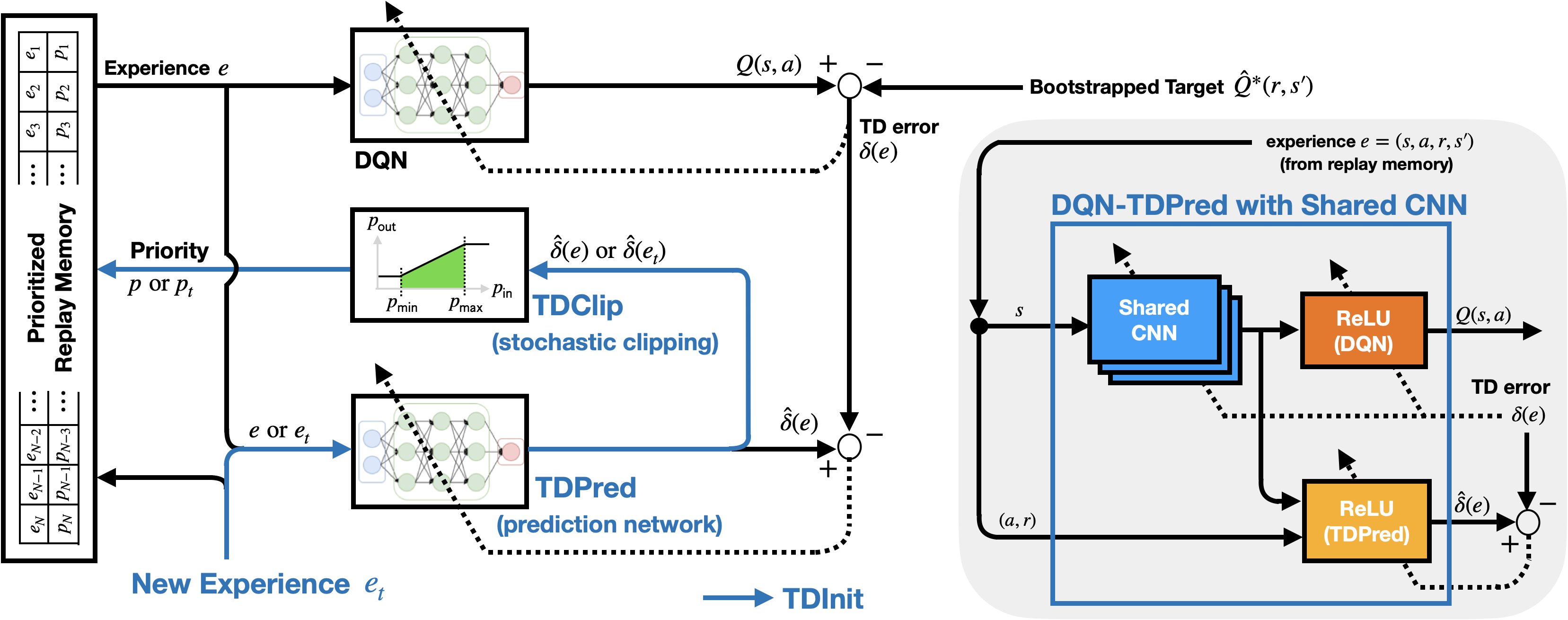
Figure 1: Overview of the proposed method, predictive PER (PPER), where the (initial) priorities are determined based on the TD-error (TDInit), its statistical clipping (TDClip), and its prediction (TDPred). TDPred reuses DQN’s convolution layers that are trained by DQL (right).

Atari Experiments

We experimentally validate the stability and performance of the three countermeasures and PPER by comparing them with PER, all applied to Atari games with double DQN and dueling network structure. We consider 5 and total 58 Atari tasks for the ablation study in Section 3 and the full evaluation in Section 4, respectively. In the experiments, $50$ millions ($=T_{\mathsf{max}}$) training steps are performed with consistent hyper-parameters (see Appendix C for details).

2 Prioritized Experience Replay, Revisited

To motivate our work, we revisit the original PER (Schaul et al., 2016). It has a prioritized replay memory $\mathscr{D}$. Each data $e\in\mathscr{D}$ has a priority $p\geq 0$; when a new experience comes and its length $N:=|\mathscr{D}|$ reaches the maximum capacity, the oldest is removed from $\mathscr{D}$. Algorithm 1 describes the DQL with PER. At each time $t=1,\cdots,T_{\mathsf{max}}$, the agent stores the observed transition tuple $e_{t}=\langle s_{t-1},a_{t-1},r_{t},s_{t}\rangle$ into $\mathscr{D}$, with its priority $p_{t}=p_{\mathsf{max}}$ (lines 1–1), where $p_{\mathsf{max}}$ denotes the largest priority ever computed (line 1); the action $a_{t-1}$ is sampled and applied to the environment, according to the distribution $\pi_{\theta}(s_{t-1})$ on the finite action space $\mathscr{A}$. The behavior policy $\pi_{\theta}$ maps each state $s$ to a distribution on $\mathscr{A}$ and typically depends on the DQN $Q_{\theta}$ (e.g., $\epsilon$-greedy).

Every $t_{\mathsf{replay}}$ instant, a batch of a $K$-number of transitions $e=\langle s,a,r,s^{\prime}\rangle$’s are sampled from $\mathscr{D}$, from the experience distribution $\mathrm{Dist}_{\mathscr{D}}$ on $\mathscr{D}$ defined by the priorities as

$$\mathrm{Dist}_{\mathscr{D}}(i)\,:=\,p_{i}^{\alpha}\,\big{/}\,{\smash{\textstyle\sum_{j=1}^{N}}p_{j}^{\alpha}}\qquad\quad(\alpha\in[0,1])$$ (1)

at each index $i=1,\cdots,N$. The selected batch is then used to calculate the gradient $\nabla_{\theta}Q_{\theta}(s,a)$ and the TD error $\delta(e)={\hat{Q}}^{*}(s^{\prime},r;\theta,\theta^{-})-Q_{\theta}(s,a)$, by which the agent updates all the batch priorities $p$’s, the largest priority $p_{\mathsf{max}}$ ever computed, and with importance sampling (IS), the DQN weights $\theta$ (lines 1–1). The priority $p$ is updated proportionally to $|\delta|$ (line 1). The bootstrapped target $\hat{Q}^{*}(r,s^{\prime};\theta,\theta^{-}):=r+\gamma\cdot Q_{\theta^{-}}(s^{\prime},\textstyle\operatorname*{arg\,max}_{a^{\prime}\in\mathscr{A}}Q_{\theta}(s^{\prime},a^{\prime}))$ (Van Hasselt et al., 2016), where $Q_{\theta^{-}}$ is the target DQN that has the same structure as $Q_{\theta}$, with its weights $\theta^{-}$. Every $t_{\mathsf{target}}$ instant, the target DQN $Q_{\theta^{-}}$ copies the DQN weights $\theta$, i.e., $\theta^{-}\leftarrow\theta$ (line 1). This happens with a large enough $t_{\mathsf{target}}$, e.g., $t_{\mathsf{target}}=\smash{10^{4}}$ and $t_{\mathsf{replay}}=4$ in our experiments and Schaul et al. (2016)’s.

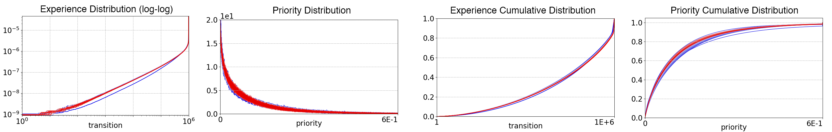
(a) Seaquest, a good example

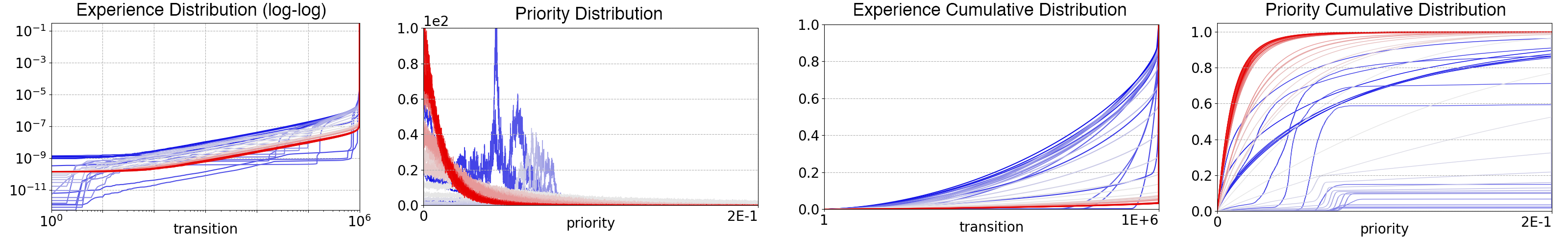
(b) Zaxxon, a bad example

Figure 2: (Cumulative) distributions in PER, from blue ($t=1$) to red $(t=T_{\mathsf{max}}$).

For notational convenience, we assume without loss of generality that the priorities are sorted, so that $p_{i}\leq p_{j}$ and thus $\mathrm{Dist}_{\mathscr{D}}(i)\leq\mathrm{Dist}_{\mathscr{D}}(j)$ if $i\leq j$. Similarly, $p_{i_{k}}\!\leq p_{i_{l}}$ for any batch $\langle p_{i_{k}}\rangle_{k=1}^{K}$ if $k\leq l$. With this convention, the last priorities $p_{N}$ and $p_{i_{K}}$ denote the maximum priorities $\max_{1\leq i\leq N}p_{i}$ in the memory $\mathscr{D}$ and $\max_{1\leq k\leq K}p_{i_{k}}$ in the batch, respectively. We also define priority distribution $\mathscr{P}_{\mathscr{D}}(p):=\smash{\sum_{i=1}^{N}}\mathbb{1}(p=p_{i})/N$, where $\mathbb{1}(\cdot)$ is the indicator function. Both distributions $\mathrm{Dist}_{\mathscr{D}}$ and $\mathscr{P}_{\mathscr{D}}$ are the main topic of this work. Figure 2 shows the (a) good and (b) bad examples of those distributions (left) in PER and their cumulative ones (right).

Experience sampling (line 1) is central to PER. It provides a trade-off between priority and diversity of samples. At one extreme, if $\mathrm{Dist}_{\mathscr{D}}=1/N$ (i.e., $\alpha=0$ or $p_{i}$’s are all the same for all $i$), then PER is of no effect and reduced to uniform sampling (maximum diversity, minimum prioritization). On the other hand, if $\mathrm{Dist}_{\mathscr{D}}(i)=\mathbb{1}(p_{i}=p_{N})/N^{\prime}$ for $N^{\prime}:=N\!\cdot\!\mathscr{P_{D}}(p_{N})$, then PER always chooses the experiences that have the maximum priority $p_{N}$ (minimum diversity). Equation 1 lies in between these two extremes, balancing priority and diversity of sampled data. Here, we note that an adequate level of diversity in the samples can be a key to stable DRL — if the diversity is too low, then the agent would use just a tiny highly-prioritized subset of $\mathscr{D}$ and never sample any of the other experiences in $\mathscr{D}$ for a long time, starting to (slowly) forget what it has already learned! Figure 2(b) (e.g., see middle-right) shows such an example, where transitions to the impulsive experience distribution results in disastrous loss of diversity in samples, leading to severe forgetting, eventually. In short, PER needs to maintain a certain level of diversity of experience samples to prevent such forgetting. The proposed PPER and its three countermeasures (TDInit, TDClip, TDPred) are designed for such purpose.

1 Initialize: the DQN weights $\theta$; the target DQN weights $\theta^{-}\leftarrow\theta$;

2 Observe an initial state $s_{0}$; set the replay memory $\mathscr{D}=\varnothing$ and $p_{\mathsf{max}}\leftarrow 1$;

3 for $t=1\;\mathrm{to}\;T_{\mathsf{max}}$ do

4       Apply an action $a_{t-1}\sim\pi_{\theta}(s_{t-1})$ and observe the reward $r_{t}$ and the next state $s_{t}$;

5       Store the experience $e_{t}:=\langle s_{t-1},a_{t-1},r_{t},s_{t}\rangle$ into $\mathscr{D}$, with its priority $p_{t}\leftarrow p_{\mathsf{max}}$;

6       if $t\emph{ mod }t_{\mathsf{replay}}=0$  then $\Delta\leftarrow 0$;

7             for $k=1\;\mathrm{to}\;K$ do

8                   Sample a transition index $i_{k}\sim\mathrm{Dist}_{\mathscr{D}}(\cdot)$ of $\mathscr{D}$ (Equation 1);

9                   Compute the IS weight $w_{k}\leftarrow(N\cdot\mathrm{Dist}_{\mathscr{D}}(i_{k}))^{-1}$;

10                   Get the experience $e:=\langle s,a,r,s^{\prime}\rangle\in\mathscr{D}$ at the index $i_{k}$;

11                   Compute the TD error $\delta\leftarrow{\hat{Q}}^{*}(r,s^{\prime};\theta,\theta^{-})-Q_{\theta}(s,a)$;

12                   Update the priority $p\leftarrow|\delta|$ at the index $i_{k}$ of $\mathscr{D}$; then, set $p_{\mathsf{max}}\leftarrow\max\{p_{\mathsf{max}},p\}$;

13                   Accumulate the weight update: $\Delta\leftarrow\Delta+\smash{w_{k}^{\beta}}\cdot\delta\cdot\nabla_{\theta}Q_{\theta}(s,a)$;

14                  

15             Update the weights $\theta\leftarrow\theta+\eta\cdot\Delta\big{/}\big{(}\max_{k}w_{k}^{\beta}\big{)}$;

16            

17       $\theta^{-}\leftarrow\theta$ if $t\text{ mod }t_{\mathsf{target}}=0$;

18      

Algorithm 1 Prioritized Experience Replay (Schaul et al., 2016)

2.1 Priority Outliers and Explosions

Priority outliers are experiences with extremely large or small priorities: they make the experience distribution $\mathrm{Dist}_{\mathscr{D}}(i)$ towards $\mathbb{1}(p_{i}=p_{N})/N^{\prime}$, losing diversity in samples hence stability of the DQN, as discussed above. Priority explosions refer to abrupt increases of priorities over time: they generate a bulky amount of extremely large priorities in a period of time, making the current priorities relatively but extremely small, hence resulting in a massive amount of priority outliers, with unstable priority and experience distributions. Once the explosion happens, the DQN weights $\theta$ can rapidly change since $\mathrm{Dist}_{\mathscr{D}}$ and thus the DQN inputs do. If the behavior policy $\pi_{\theta}$ becomes significantly different or bad accordingly, then there would become no way to recover the past experiences, meaning that the DQN will be forgetting what it has already learned, on and on. Figures 2(b) (right-most, blue curves) and 5(d) (high variance TD error) illustrate such outliers in PER and when the explosion happens, respectively.

The main working hypothesis of the current paper is that, for the above reasons, priority outliers and explosions should be avoided. We shall now discuss how they occur in PER.

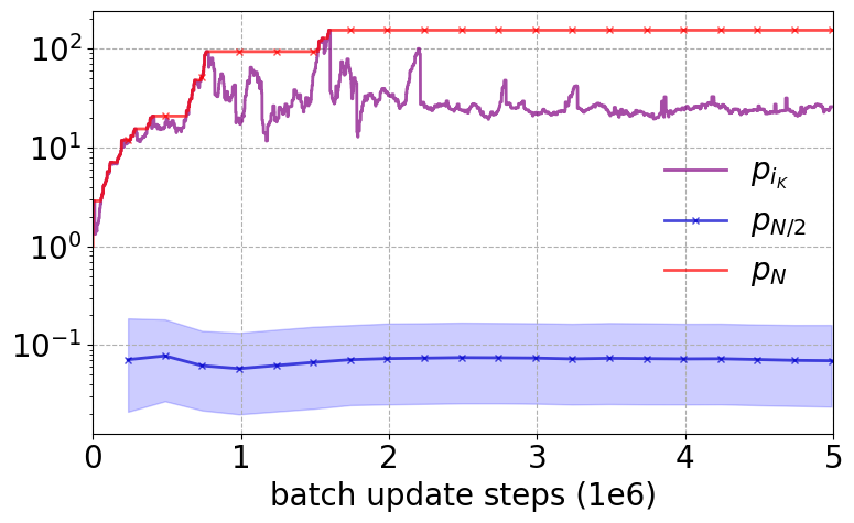
Figure 3: Smoothed trajectories of priorities $p_{i_{K}}$, $p_{\lceil N/2\rceil}$, and $p_{N}$ (Seaquest).

Choice of Initial Priorities

Our first observation is that the choice of an initial priority in PER causes priority outliers. According to line 1, the initial priority $p_{t}$ is the largest priority $p_{\mathsf{max}}$ ever computed in the PER that is in general an upper bound of the priority maximum $p_{N}$. In PER, $p_{N}=p_{\mathsf{max}}$ always since the initial priorities $p_{t}$’s set to $p_{\mathsf{max}}$ come into play (line 1). However, the TD error $|\delta|$, and thus the priorities $p$’s once updated by $p\leftarrow|\delta|$ (line 1), eventually become much smaller, as training progresses and comes to stabilization. Moreover, by the update $p_{\mathsf{max}}\leftarrow\max\{p_{\mathsf{max}},p\}$ (line 1), $p_{\mathsf{max}}$ can ever increase. As a consequence, $p_{\mathsf{max}}$ and thus all initial priorities $p_{t}$’s can become extremely large and out of the current priority distribution (e.g., see Figures 2(b)), meaning that they act as priority outliers. The experimental result in Figure 3 supports this claim: it shows the trajectory of $p_{\mathsf{max}}$ ($=p_{N}$) and the transition of the median priority $p_{\lceil N/2\rceil}$. We see the large gap between the two, and that $p_{\mathsf{max}}$ never decreases even though the maximal priority $p_{i_{K}}$ in the batch (violet) starts to decrease at early steps. TDInit provides a solution for this issue due to the ever increasing $p_{\mathsf{max}}$ (lines 1 and 1).

Distributions and Spikings of TD-errors

TD errors, thus priorities, have a distribution that is dense near zero, as shown in Figure 2(a) and (b) (see middle-left). Such a distribution can induce lots of experiences with almost zero priorities that are useless as they are almost never sampled (de Bruin et al., 2018). The other issue is that the TD error $\delta$ can spike. Spikes in $\delta$ affect both the initial priorities, by making $p_{\mathsf{max}}$ larger, and the batch priority update (lines 1 and 1), both causing priorities to spike. Such spikes typically occur with (i) new experiences that have not explored or well-exploited yet and (ii) old ones that were not replayed for a long time; then, the TD errors $|\delta|$’s tend to be initially very high or different from the previous’, respectively. Figure 3 shows that this is indeed the case: for example, the maximal batch priority $p_{i_{K}}$ are seen to be far above the median priority $p_{\lceil N/2\rceil}$ in $\mathscr{D}$. A series of TD-error spikes dense-in-time can rapidly ruin the sample diversity thus induce a priority explosion. This is especially when the agent learns a new task or stays in a region that is not explored before. In this case, most of the new TD-errors are expected to be large relative to the old ones, hence may act as spikes, eventually losing lots of past data without sampling them enough. We use two ideas to alleviate this difficulty: TDClip and TDPred.

3 Predictive Prioritized Experience Replay

We made a hypothesis: priority outliers and explosions harm the stability of PER. We now introduce the three countermeasures for reducing them: TD-error-based initial priorities (TDInit), statistical TD-error clipping (TDClip), and TD-error prediction network (TDPred). Their combination constitutes our proposed Predictive PER (PPER). In this section, PPER and each idea are experimentally evaluated via ablation study on 5 Atari games as shown in Figures 4 and 6 (see Appendix D for more).

3.1 TDInit: TD-error-based Initial Priorities

A possible way of avoiding the outliers—resulting from $p\leftarrow p_{\mathsf{max}}$—is to take the current median priority $p_{\lceil N/2\rceil}$, replacing line 1 with $p_{t}\leftarrow p_{\lceil N/2\rceil}$. TDInit is more informative: it takes $|\delta_{t}|$ as the initial priority. Therefore, line 1 becomes $p_{t}\leftarrow|\delta_{t}|$ that is now the same as the batch priority update rule (line 1). With this modification, the TD errors $|\delta|$’s and thus the maximal priority $p_{N}$ are expected to decrease as the training goes on and on, whereas $p_{N}$ ($=p_{\mathsf{max}}$) in PER never decreases.

As shown in Figure 4, TDInit can resolve severe forgetting of PER (BattleZone; Robotank) or even improve overall performance (Robotank; Seaquest). However, TDInit alone may not be enough since other types of priority outliers can occur, which cause priority explosions (e.g., TD-error spikes). Figure 4 shows such examples (Tennis; Zaxxon), where TDInit cannot prevent the severe forgetting or even make it worse. Also notice a lot of distributional variations with priority outliers and explosions (Figures 5(a) and (d), resp.). Bounding the priorities (e.g., TDClip) or reducing their (distributional) variance (e.g., TDPred) can solve or significantly alleviate such phenomena.

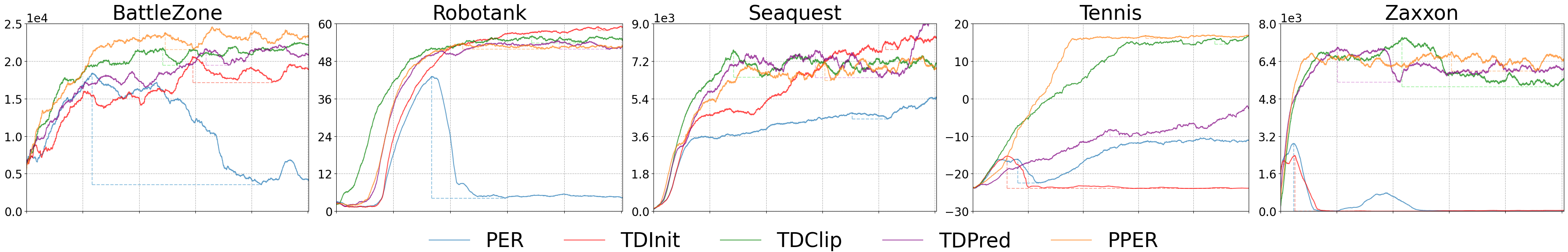
Figure 4: Training scores of PER, PPER, and the three countermeasures, up to $T_{\mathsf{max}}=50$M steps.

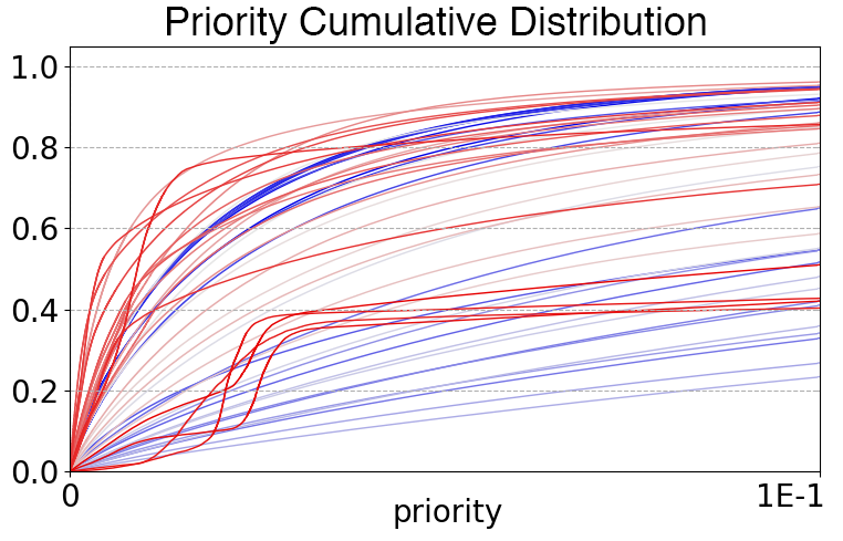
(a) TDInit, Tennis

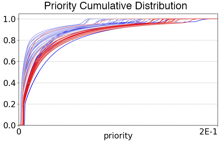
(b) TDClip, Tennis

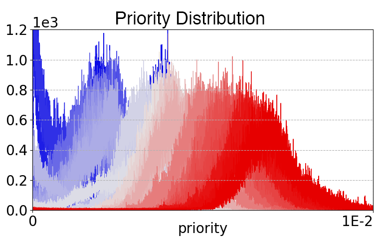
(c) TDPred , Zaxxon

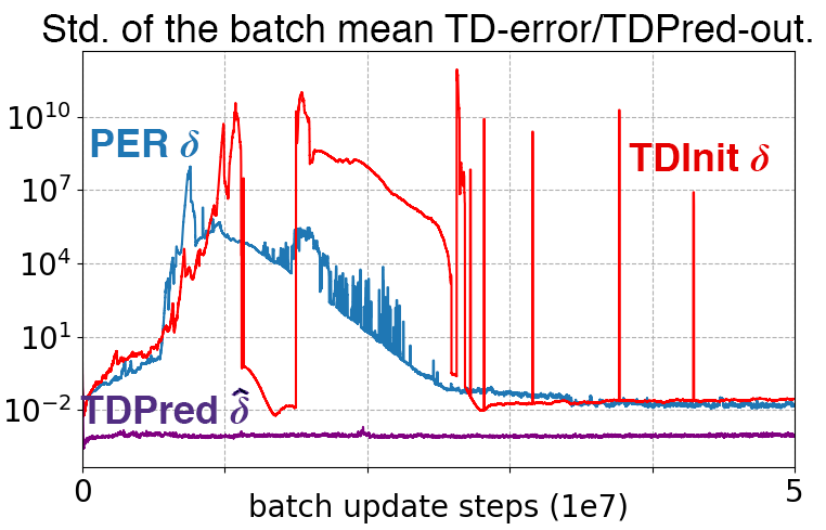
(d) Zaxxon

Figure 5: (a)–(c) Priority distributions; (d) std. of batch mean of $\delta$ (PER/TDInit) and $\hat{\delta}$ (TDPred)

3.2 TDClip: Statistical TD-error Clipping

TDClip clips the absolute TD errors to remove priority outliers. One naive approach of such is by fixed clipping bounds. However, such a scheme can be ineffective since the TD errors can be large in the beginning but tend to decrease in magnitudes. Their statistics change over the training.

To come up with such difficulty, we actively estimate the average $\mu:=\sum_{i=1}^{N}|\delta(e_{i})|/N$ of the current TD errors $|\delta(e)|$’s of all the experiences $e$ in $\mathscr{D}$. In each priority update, we use the estimate $\tilde{p}$ of $\mu$ to statistically clip the priority in its update rule: $p\leftarrow\mathrm{median}\smash{\big{\{}p_{\mathsf{min}},\,|\delta|,\,p_{\mathsf{max}}\big{\}}}$. Here, the clipping bounds $\langle p_{\mathsf{min}},p_{\mathsf{max}}\rangle$ are initialized to $\langle 0,1\rangle$ and updated to $\langle\rho_{\mathsf{min}},\rho_{\mathsf{max}}\rangle\cdot\tilde{p}$ whenever $\tilde{p}$ is updated. Our design choice is $\langle\rho_{\mathsf{min}},\rho_{\mathsf{max}}\rangle=\langle 0.12,3.7\rangle$, which makes $p_{\mathsf{min}}$ and $p_{\mathsf{max}}$ the $0.1\sigma$ and $3\sigma$ points of the distribution of TD error $\delta$ over $\mathscr{D}$ if $\delta\sim\mathcal{N}(0,\sigma)$ (Appendix B). At each batch update step $k$, we update $\tilde{p}$ with an estimate $\Delta_{\mathsf{a}}:=\sum_{k=1}^{K}w_{k}\cdot|\delta(e_{i_{k}})|/K$ of the current $\mu$ via

$$\kappa\leftarrow\lambda\cdot\kappa+1\quad\text{and then}\quad\tilde{p}\leftarrow\tilde{p}+\big{(}\Delta_{\mathsf{a}}-\tilde{p}\big{)}/\kappa$$ (2)

where both $\kappa$ and $\tilde{p}$ are initialized to zero; the forgetting factor $\lambda\in(0,1)$, which we set $\lambda=0.9985$ in all of the experiments, compensates the non-stationary nature of the TD error distribution. For more details with theoretical analysis, see Appendix B.

Figure 4 shows that TDClip prevents forgetting and thus achieves higher scores than PER’s, in all 5 Atari games including those where TDInit cannot (Tennis; Zaxxon)—TDClip effectively clips the outliers that exist in PER and TDInit as shown in Figure 5(b). Also note that by TDClip, $p_{\mathsf{max}}$ can now decrease and be located at the edge of the priority in-distribution, without TDInit.

3.3 TDPred: TD-error Prediction Network

The TD-error prediction network (TDPred) ${\hat{\delta}}\equiv\hat{\delta}_{\vartheta}$, parameterized by $\vartheta$, smoothly generalizes the in-distribution experiences in $\mathscr{D}$ with a variance-reduced Gaussian-like distribution, by minimizing the mean squared loss $L_{\mathscr{D}}(\vartheta):=\mathbb{E}_{i\sim\mathrm{Dist}_{\mathscr{D}}(\cdot)}\big{[}\,(\hat{\delta}_{\vartheta}(e_{i})-\delta(e_{i}))^{2}\,\big{]}$ in an online supervised manner, where $\delta(e)$ and $\smash{\hat{\delta}}_{\vartheta}(e)$ denote the TD error and the TDPred output, w.r.t. the input experience $e\in\mathscr{D}$. The corresponding stochastic gradient descent update is: $\vartheta\leftarrow\vartheta+\eta_{\mathsf{p}}\cdot\big{(}\delta(e_{i})-\smash{\hat{\delta}_{\vartheta}(e_{i})}\big{)}\cdot\nabla_{\vartheta}{\hat{\delta}}_{\vartheta}(e_{i})$ for a learning rate $\eta_{\mathsf{p}}$, where the index $i\sim\mathrm{Dist}_{\mathscr{D}}(\cdot)$. The idea of TDPred is to employ its output to assign the priority as $p\leftarrow|\smash{\hat{\delta}_{\vartheta}}|$, and its effect on $p$ has three folds below. In short, TDPred’s generalization capabilities allow us to smooth out TD errors—especially for new experiences on which the DQN is not trained enough—and avoid priority outliers, spikes, and explosions. Figure 4 shows that the stability is indeed enhanced as TDPred shows no severe forgetting while PER does.

Regularization

The TDPred output $\smash{\hat{\delta}}_{\vartheta}$ varies over time more slowly than the TD error $\delta$, due to its $\vartheta$-update process. Hence, the use of TDPred regularizes the abrupt distributional changes in the priorities to avoid them from being outliers and prevent their explosions (see Figure 5(c) and (d)).

Gaussian-like Priority Distribution

The output of a wide DNN is typically Gaussian (Matthews et al., 2018). Likewise, as in Figure 5(c) and Appendix D, the priority $p$ of TDPred (under small variance), updated proportionally to $|\hat{\delta}_{\vartheta}|$, has a Gaussian-like distribution, eventually — even for the case where the network is not wide, except a few (Appendices D and G). This can reduce priority outliers as the distribution is symmetric and heavily centered at the mean, whereas the power-law priority distributions in PER and TDInit are heavily tailed, skewed towards and dense near zero.

Variance Reduction

A modern analysis shows that DNNs can significantly reduce both variance of the outputs and bias from the target (Neal et al., 2018), overcoming traditional bias-variance dilemma (Geman et al., 1992). The use of TDPred therefore results in variance reduction of its outputs $\smash{\hat{\delta}}_{\vartheta}$’s (hence, the priorities $p$’s) while keeping the bias reasonably small (i.e., $\big{|}\mathbb{E}_{i\sim\mathrm{Dist}_{\mathscr{D}}(\cdot)}[\delta(e_{i})-\hat{\delta}_{\vartheta}(e_{i})]\big{|}\ll 1$). Figure 5(d) and Appendix D show that this is indeed true for all 5 Atari games — for the sampled experience $e_{i_{k}}\in\mathscr{D}$, the variances of $|\smash{\hat{\delta}}_{\vartheta}|$’s and $p$’s in TDPred are typically at least 10 times smaller than those of $|\delta|$ in PER, while keeping the error $|\smash{\hat{\delta}}_{\vartheta}|-|\delta|$ reasonably small. As a result, TDPred removes high-variance priority outliers and makes the distribution more centered and denser around the mean, making itself insensitive to large TD-error deviations hence explosions. Regarding the bias, we note that as in rank-based prioritization (Schaul et al., 2016), the high precision of the TD errors is not always necessary.

Our Design Choices We empirically found that TDPred must be a ConvNet to learn $\delta$. We let TDPred share DQN’s convolutional layers, which has two advantages: 1) establishing the common ground of two function approximators, 2) reducing computational cost of TDPred’s update. Update of TDPred is only relevant to its fully-connected layers (see Section 4 and Appendix C for more).

1 Initialize: the DQN weights $\theta$; the target network weights $\theta^{-}\leftarrow\theta$; the TDPred weights $\vartheta$;

2 Observe $s_{0}$; set the replay memory $\mathscr{D}=\varnothing$; $\kappa\leftarrow 0$ and $\langle p_{\mathsf{min}},\;\tilde{p},\;p_{\mathsf{max}}\rangle\leftarrow\langle 0,0,1\rangle$;

3 for $t=1\;\mathrm{to}\;T_{\mathsf{max}}$ do

4       Apply an action $a_{t-1}\sim\pi_{\theta}(s_{t-1})$ and observe the reward $r_{t}$ and the next state $s_{t}$;

5       Compute TDPred output ${\hat{\delta}}_{t}\leftarrow{\hat{\delta}}_{\vartheta}(e_{t})$ for the transition $e_{t}:=\langle s_{t-1},a_{t-1},r_{t},s_{t}\rangle$;

6       Compute priority $p_{t}\leftarrow\mathrm{median}\big{\{}p_{\mathsf{min}},\,|\smash{\hat{\delta}}_{t}|,\,p_{\mathsf{max}}\big{\}}$ and store $(e_{t},p_{t})$ in $\mathscr{D}$;

7       if $t\emph{ mod }t_{\mathsf{replay}}=0$ then $\langle\Delta_{\mathsf{q}},\Delta_{\mathsf{p}},\Delta_{\mathsf{a}}\rangle\leftarrow\langle 0,0,0\rangle$;

8             for $k=1\;\mathrm{to}\;K$  do

9                   Sample a transition index $i_{k}\sim\mathrm{Dist}_{\mathscr{D}}(\cdot)$ and compute $w_{k}\leftarrow(N\cdot\mathrm{Dist}_{\mathscr{D}}(i_{k}))^{-1}$;

10                   Get the experience $e:=\langle s,a,r,s^{\prime}\rangle\in\mathscr{D}$ at the index $i_{k}$;

11                   Compute TD error $\delta\leftarrow{\hat{Q}}_{*}(r,s^{\prime};\theta,\theta^{-})-Q_{\theta}(s,a)$ and TDPred output ${\hat{\delta}}\leftarrow{\hat{\delta}}_{\vartheta}(e)$;

12                   Update the priority $p\leftarrow\mathrm{median}\big{\{}p_{\mathsf{min}},\,|\smash{\hat{\delta}}|,\,p_{\mathsf{max}}\big{\}}$ at the index $i_{k}$ of $\mathscr{D}$;

13                   $\big{\langle}\Delta_{\mathsf{a}},\Delta_{\mathsf{p}},\Delta_{\mathsf{q}}\big{\rangle}\leftarrow\big{\langle}\Delta_{\mathsf{a}},\Delta_{\mathsf{p}},\Delta_{\mathsf{q}}\big{\rangle}\,+\,\big{\langle}w_{k}\cdot|\delta|/K,\;\;(\delta-\hat{\delta})\cdot\nabla_{\vartheta}{\hat{\delta}}_{\vartheta}(e),\;\;w_{k}^{\beta}\cdot\delta\cdot\nabla_{\theta}Q_{\theta}(s,a)\big{\rangle}$;

14                  

15             Update the weights $\theta\leftarrow\theta+\eta_{\mathsf{q}}\cdot\Delta_{\mathsf{q}}\big{/}\big{(}\max_{k}w_{k}^{\beta}\big{)}$ and $\vartheta\leftarrow\vartheta+\eta_{\mathsf{p}}\cdot\Delta_{\mathsf{p}}$;

16             Update $\kappa$ and then $\tilde{p}$ via Equation 2; then, set $\langle p_{\mathsf{min}},p_{\mathsf{max}}\rangle\leftarrow\langle\rho_{\mathsf{min}},\rho_{\mathsf{max}}\rangle\cdot\tilde{p}$;

17            

18       $\theta^{-}\leftarrow\theta$ if $t\text{ mod }t_{\mathsf{target}}=0$;

19      

Algorithm 2 Predictive Prioritized Experience Replay (PPER)

3.4 PPER, A Stable Priority Updater

Our proposal, PPER, combines the above three countermeasures, each of which increases sample diversity (i.e., making the distribution $\mathrm{Dist}_{\mathscr{D}}(i)$ away from $\mathbb{1}(p_{i}=p_{N})/N^{\prime}$ but towards $1/N$ in a degree) and thus contributes to stability of the prioritized DQN. The pseudo-code of PPER is provided in Algorithm 2. As PPER inherits the features and properties of the three countermeasures, it is expected that PPER can best stabilize the DQN although not best performing, as shown in Figure 4, due to the loss of prioritization at the cost of increasing sample diversity.

To quantify stability for each case and PPER, we evaluated the $\mathrm{normalized\_max\_forget}$ measure:

$$\mathrm{normalized\_max\_forget}:=\frac{\mathrm{score}(t_{T^{*}})-\min_{t_{T^{*}}\leq t\leq T_{\mathsf{max}}}\mathrm{score}(t)}{\mathrm{score}(t_{T^{*}})-\min_{1\leq t\leq T_{\mathsf{max}}}\mathrm{score}(t)}\in[0,1],$$ (3)

where $\mathrm{score}(t)$ is the game score on a learning curve in Figure 4, $t_{T}:=\textstyle\operatorname*{arg\,max}_{1\leq t\leq T}\mathrm{score}(t)$ denotes the first time at which the score becomes the maximum within the horizon $T\leq T_{\mathsf{max}}$, and $T^{*}$ is the horizon $T$ at which the $\mathrm{forget}(T):=\mathrm{score}(t_{T})-\textstyle\min_{t_{T}\leq t\leq T_{\mathsf{max}}}\mathrm{score}(t)$ is maximized. The numerator of Equation 3 is equal to $\mathrm{forget}(T^{*})$, the score the agent maximally forgets during the training; the denominator normalizes it by the gap between $\mathrm{score}(t_{T^{*}})$ and the minimum score. Note that $\mathrm{normalized\_max\_forget}=1$ means that the agent at the end has forgot everything it had learned; it is zero when no forgetting observed on a training curve. For each case, the vertical dotted line in Figure 4 indicates the $\mathrm{forget}(T^{*})$.

Figure 6(a) presents the normalized maximum forgets (Equation 3) of PER, the three countermeasures (TDInit, TDClip, TDPred), their combinations (TDInitPred, TDInitClip, TDClipPred), and PPER, in percents. PER showed the severe forgetting in 4 out of 5 games (i.e., except Seaquest), whereas all the forgetting metrics of the proposed countermeasures, their combinations, and PPER, except TDInit (Tennis; Zaxxon) and TDInitPred (Tennis), remain within around 25% as shown in Figure 6(a). Overall, PPER is the minimum among them. Except TDInit, the average learning performance of all cases are better than PER as summarized in Figure 4(b); PPER gives higher average scores than any other cases but TDClipPred. We note that (i) the four (resp. two) best-performing ones in Figure 4(b) all combine TDClip (resp. TDClip and TDPred); (ii) combined with TDPred, the priorities at the end always show a variance-reduced Gaussian-like distribution (Appendix D). More ablation study (e.g., TDClipPred/TDInit) remains as a future work.

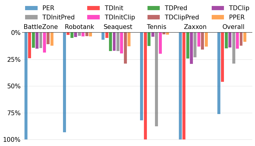
(a) Normalized Maximum Forgets

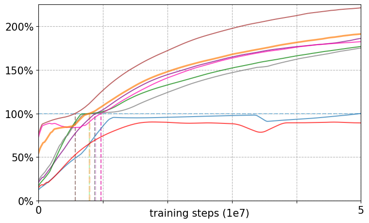
(b) The Median of Mean Scores, PER-normalized

Figure 6: Summary of ablation study. (a) normalized maximum forgets for all cases; (b) the medium over 5-games of each average of the scores so far, normalized by PER.

4 Experiments on Atari 2600 Environments

Through Atari experiments, we evaluate stability and performance of PPER, relative to the original PER, the baseline. The result shows that PPER indeed improves the stability during training with the test score also higher than PER on the average. We designed the TDPred in a way that its convolutional layers, shared with the DQN, are followed by a fully-connected layer with $M$-neurons. Details on the experimental settings are provided in Appendix C. In the first place, we experimented the total 58 Atari games with $M=512$ and the results are shown in Figures 7, 8(a), and 8(b).

Stability

We first see how much the stability of PPER is improved, by measuring

$$\mathrm{relative\_stability\_score}:=\mathrm{normalized\_max\_forget}_{\mathsf{PER}}-\mathrm{normalized\_max\_forget}_{\mathsf{PPER}}$$

where $\mathrm{normalized\_max\_forget}_{m}$ is the normalized maximum forget, given by Equation 3, of the prioritization method $m$, with the $\mathrm{score}$’s coming from its training histories (see Appendix E). If relative stability score is $1$, then it means that PER completely forgets whereas the PPER never, and vice versa if $\mathrm{relative\_stability\_score}=-1$. A positive relative stability score indicates that PPER less forgets than PER. As shown in Figure 7(a), PPER less forgets in 42 out of 58 games, with $\mathrm{relative\_stability\_score}\approx 23.2\%$ on the average. In Appendix H, one can see that PPER indeed reduces the variance of the priorities, which can improve the sample diversity, hence stability.

Training Performance

Figure 8 shows (a) the median over 53 games of maximum PER-normalized scores achieved so far, and (b) the same as (a) but with the maximum replaced by average. Both represent the peak and the average performance over the training steps, respectively (see also Schaul et al., 2016, Figure 4). It is clear that the average performance growth of PPER has been improved notably, as it reaches at the same level of PER’s at 45% of the total training steps approximately, but the peak performance in Figure 8(a) has not. From the training curves in Appendix E, we observed that this is mainly from the stabilized training of PPER—PER can reach more or less the same maximum score as PPER (similar peak performance), but since PER forgets (sometimes severely), its average performance goes down.

Evaluation via Testing We evaluate the learned policies in relative test scores, which measures the performance gap between PER and PPER with each game’s difficulty taken into account:

$$\mathrm{relative\_test\_score}:=\frac{(\mathrm{score_{\mathsf{PPER}}}-\mathrm{score_{\mathsf{PER}}})}{\max\{\mathrm{score_{\mathsf{Human}}},\mathrm{score_{\mathsf{PER}}}\}-\mathrm{score_{\mathsf{Random}}}}.$$

Here $\mathrm{score_{\mathsf{PPER}}}$ and $\mathrm{score_{\mathsf{PER}}}$ are corresponding test scores, $\mathrm{score_{\mathsf{Human}}}$ and $\mathrm{score_{\mathsf{Random}}}$ are the human- and random-play scores reported by Wang et al. (2015). For $\mathrm{score_{\mathsf{PPER}}}$ and $\mathrm{score_{\mathsf{PER}}}$, we take the average score over 200 repetitions of the no-ops start test with the best-performing model (Mnih et al., 2015; Van Hasselt et al., 2016). From Figure 7(b), we observed that policies are improved in PPER on 34 of 53 games. For those games, we found that its training curves are mainly either gradually increasing without, or less suffering from forgettings. Also, unlike PER, priority distributions of PPER are Gaussian-like, where priority outliers and explosion are removed. As we claimed above, such a difference is the key to balance priority and diversity in experience sampling, which eventually contributes to stabilized, efficient training (See Appendices D for Gaussian-like priority distributions of PPER and F for full test scores)

Stability and Performance When $M$ is Smaller In this second experiment, we trained the DQN with PPER over 15 Atari games under the same experimental settings as above, except that the number $M$ of the neurons in TDPred’s fully-connected layer is reduced to 256, 128, 64 and 32. Figures 8(c) and (d) summarize training of those variations in median scores, which can answer “No” to: “If the TDPred becomes simpler, then will it terribly affects the performance?” Indeed, Figure 8(d) shows that for all such variations, the training efficiency has been improved on the average, even when $M=32$, the minimum. Moreover, except for a few case(s) with $M=32$, the priority distributions are still Gaussian-like with no explosion or no significant outliers, meaning that PPER with much smaller TDPred can also enhance stability of training. The learning curves in Appendix G clearly show PPER in this case has higher scores and forgets less than PER.

However, the priority distributions of those variations are not identical, which potentially changes the level of diversity PPER pursues. In DemonAttack, for example, $M=32$ performed best among all the variations probably because its weakest diversity pursuing behavior helps it focus priority the most. Consequently, $M$ is a hyper-parameter of PPER, which trades off prioritization, sample diversity, and complexity. Regarding complexity, the training cost of TDPred reported in Table 2 (Appendix G) is about 10.9% of DQN’s for $M=512$ and 6.6% for $M=128$, which are significantly less than DQN’s, thanks to our design choice. See Appendix G for details of the experiment.

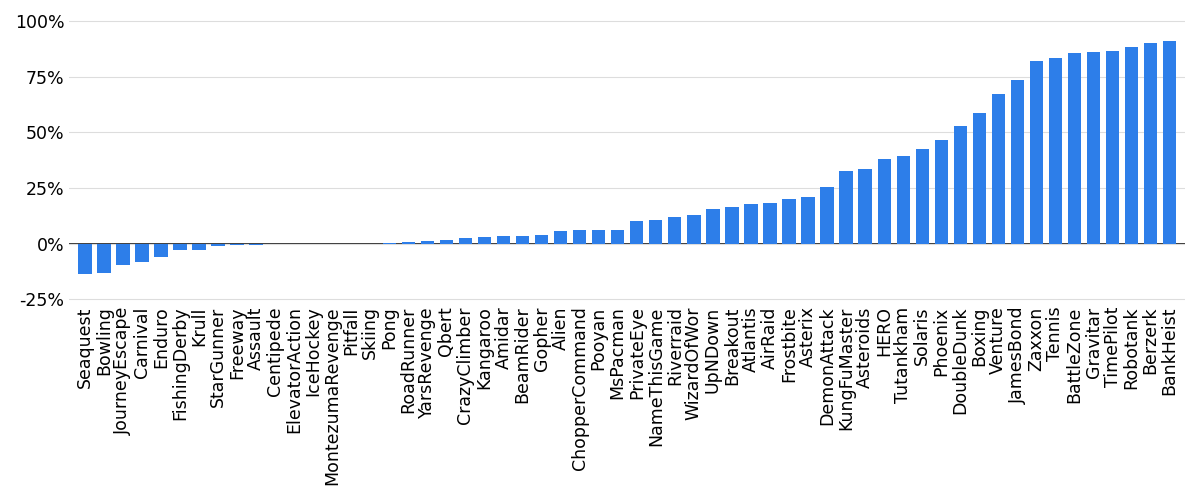
(a) Relative stability scores (58 games)

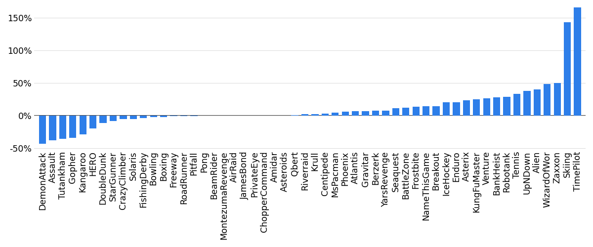
(b) Relative test scores (53 games)

Figure 7: Stability and test scores of PPER relative to PER in percents, trained up to 50M frames.

(a) Median Max Score

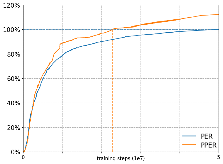
(b) Median Avg Score

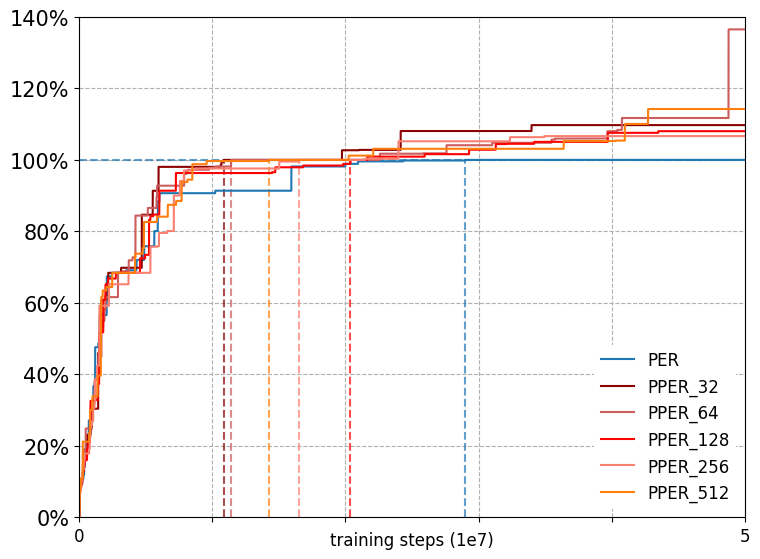
(c) Median Max Score

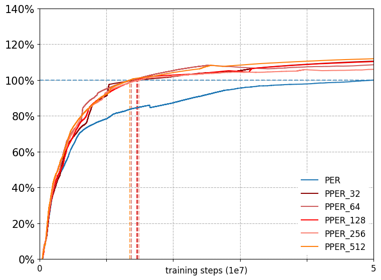
(d) Median Avg Score

Figure 8: Summary of training over 53 games (a, b) / over 15 games with smaller $M$’s (c, d).

5 Conclusions

This paper proposed predictive PER (PPER) which combines three countermeasures (TDInit, TDClip, and TDPred) designed to effectively remove the outliers, spikes, and explosions of priorities for balancing diversity of samples over prioritization. Ablation and full experimental studies with Atari games justified our claim: a certain level of diversity should be kept for maintaining stability. The experimental results showed PPER improves both performance and notably, stability. The authors believe that the proposed methods can be served as ingredients for building stable DRL systems.

Acknowledgments

The authors gratefully acknowledge the support of the Japanese Science and Technology agency (JST) ERATO project JPMJER1603: HASUO Metamathematics for Systems Design.

Appendix A Related Works.

ER and Its Extensions

ER has been employed in deep Q-learning (Mnih et al., 2013; 2015), its extensions (Wang et al., 2015; Van Hasselt et al., 2016), and the other DRL methods (Lillicrap et al., 2015; Wang et al., 2016), as an essential ingredient for providing un-correlated experiences and improving stability and sample efficiency. Several state-of-the-art extensions exist such as hindsight ER (Andrychowicz et al., 2017), curiosity-driven ER (Zhao & Tresp, 2019), ER optimization (Zha et al., 2019), distributed ER (Nair et al., 2015), and our focus, PER (Schaul et al., 2016). Other researchers have also investigated the effects of ER, and its components, on (D)RL (de Bruin et al., 2015; 2018; van Seijen & Sutton, 2015; Zhang & Sutton, 2017; Pan et al., 2018).

PER and Underlying Ideas

Many researchers have utilized PER in DRL methods — DQN and its extensions (Schaul et al., 2016; Wang et al., 2015; Hessel et al., 2018; Hester et al., 2018) and others (Wang et al., 2016; Hou et al., 2017; Vecerik et al., 2017) — for more efficient experience sampling in replay. The underlying idea of PER is known as prioritized sweeping, which prioritizes the samples in proportion to their absolute TD errors. The idea was originally applied to reinforcement planning, e.g., Dyna-Q (Sutton & Barto, 2018), and value iteration (Moore & Atkeson, 1993; Andre et al., 1998).

Extensions of PER

PER has been extended by storing and sampling the experiences from either the demonstration (Vecerik et al., 2017; Hester et al., 2018), or the distributed actors (Horgan et al., 2018). Brittain et al. (2019) proposed the Prioritized Sequence ER (PSER), which also extends the idea of PER. All of those extensions were provided with their promising experimental performance on Atari and/or continuous control tasks. PSER additionally updates all the priorities along the backward-in-time trajectory of each transition currently sampled. When updating the priorities, PSER tries to prevent the priorities from going suddenly small by slowly decaying them. In PPER, the same purpose is served by TDPred and lower-clipping in TDClip (Sections 3.2 and 3.3).

Appendix B Details on TDClip

This appendix describes the details of TDClip: (i) the update rule (Equation 2) of the estimate $\tilde{p}$ of $\sum_{i=1}^{N}|\delta(e_{i})|/N$, and (ii) the hyper-param setting $\langle\rho_{\mathsf{min}},\rho_{\mathsf{max}}\rangle=\langle 0.12,3.7\rangle$.

B.1 Estimating the Average Absolute TD-error in $\mathscr{D}$

The update rule (Equation 2) of the estimate $\tilde{p}$ can be rewritten as

$$\kappa_{n+1}=\lambda\cdot\kappa_{n}+1\quad\text{and then}\quad{\tilde{p}}_{n+1}={\tilde{p}}_{n}+\big{(}{\hat{\mu}}_{n+1}-{\tilde{p}}_{n}\big{)}/\kappa_{n+1},$$ (B.1)

where $\kappa_{n}$ and ${\tilde{p}}_{n}$ denote $\kappa$ and $\tilde{p}$ at the $n$th batch update, respectively; $\lambda\in(0,1)$ is the forgetting factor; $\textstyle{\hat{\mu}}_{n}:=\Delta_{a}$ is the estimate of $\mu_{n}:=\sum_{i=1}^{N}|\delta(e_{i})|/N$, the true average absolute TD error over the replay memory $\mathscr{D}$, at the $n$th batch update. Note that $\Delta_{a}=\sum_{k=1}^{K}w(i_{k})\cdot|\delta(e_{i_{k}})|/K$, where $w(i):=(N\cdot\mathrm{Dist}_{\mathscr{D}}(i))^{-1}$, and that by the initializations of $\kappa$ and ${\tilde{p}}$, we have $\kappa_{0}={\tilde{p}}_{0}=0$.

Note that the TD-error $\delta$, the IS weight $w$, and the replay memory $\mathscr{D}$ are typically varying over the batch update step $n$ since at every batch step, updated are the weights $\theta$ and $\theta^{-}$ of the DQNs and the experiences and priorities in $\mathscr{D}$. For notational simplicity, however, we made their dependency on the batch step $n$ implicit.

Lemma B.1.

For each $n\in\mathbb{N}$, ${\hat{\mu}}_{n}$ is an unbiased estimator of $\mu_{n}$.

Proof.

Fix $n\in\mathbb{N}$ and note that by the IS weight $w(i):=(N\cdot\mathrm{Dist}_{\mathscr{D}}(i))^{-1}$,

$$\mathbb{E}_{i\sim\mathrm{Dist}_{\mathscr{D}}(\cdot)}\Big{[}w(i)\cdot|\delta(e_{i})|\Big{]}=\sum_{i=1}^{N}\mathrm{Dist}_{\mathscr{D}}(i)\cdot w(i)\cdot|\delta(e_{i})|=\frac{1}{N}\sum_{i=1}^{N}|\delta(e_{i})|=\mu_{n}.$$

Since each index $i_{k}$ in the batch is sampled from $\mathrm{Dist}_{\mathscr{D}}(\cdot)$, we have

$$\mathbb{E}\big{[}{\hat{\mu}}_{n}\big{]}=\sum_{k=1}^{K}\mathbb{E}_{i_{k}\sim\mathrm{Dist}_{\mathscr{D}}(\cdot)}\Big{[}w(i_{k})\!\cdot|\delta(e_{i_{k}})|\Big{]}/K=\mu_{n}\cdot\sum_{k=1}^{K}1/K=\mu_{n},$$

which completes the proof. ∎

Lemma B.2.

For each $n\in\mathbb{N}$, ${\tilde{p}}_{n}=\dfrac{{\hat{\mu}}_{n}+\lambda\cdot{\hat{\mu}}_{n-1}+\cdots+\lambda^{n-1}\cdot{\hat{\mu}}_{1}}{1+\lambda+\cdots+\lambda^{n-1}}=\dfrac{\sum_{m=0}^{n-1}\lambda^{m}\cdot{\hat{\mu}}_{n-m}}{\sum_{m=0}^{n-1}\lambda^{m}}$.

Proof.

First, note that $\kappa_{n}=\sum_{m=0}^{n-1}\lambda^{m}$ since $\kappa_{1}=1$ and

$$\kappa_{n}=\lambda\kappa_{n-1}+1=\lambda^{2}\kappa_{n-2}+(\lambda+1)=\cdots=\lambda^{n-1}\kappa_{1}+(\lambda^{n-2}+\lambda^{n-3}+\cdots+\lambda+1).$$

Hence, extending ${\tilde{p}}_{n}$ in a similar manner, we obtain:

$$\kappa_{n}\cdot{\tilde{p}}_{n} =\kappa_{n}\cdot{\tilde{p}}_{n-1}+({\hat{\mu}}_{n}-{\tilde{p}}_{n-1})$$

$$={\hat{\mu}}_{n}+(\kappa_{n}-1)\cdot{\tilde{p}}_{n-1}$$

$$={\hat{\mu}}_{n}+\lambda\cdot\kappa_{n-1}\cdot{\tilde{p}}_{n-1}$$

$$={\hat{\mu}}_{n}+\lambda\cdot{\hat{\mu}}_{n-1}+\lambda^{2}\cdot\kappa_{n-2}\cdot{\tilde{p}}_{n-2}$$

$$={\hat{\mu}}_{n}+\lambda\cdot{\hat{\mu}}_{n-1}+\lambda^{2}\cdot{\hat{\mu}}_{n-2}+\lambda^{3}\cdot\kappa_{n-3}\cdot{\tilde{p}}_{n-3}$$

$$\;\,\vdots$$

$$={\hat{\mu}}_{n}+\lambda\cdot{\hat{\mu}}_{n-1}+\lambda^{2}\cdot{\hat{\mu}}_{n-2}+\lambda^{3}\cdot{\hat{\mu}}_{n-3}+\cdots+\lambda^{n-1}\cdot\kappa_{1}\cdot{\tilde{p}}_{1}.$$

This completes the proof since $\kappa_{n}=\sum_{m=0}^{n-1}\lambda^{m}$, $\kappa_{1}=1$, and ${\hat{\mu}}_{1}={\tilde{p}}_{1}$. ∎

Theorem B.1.

For each $n\in\mathbb{N}$, $\mathbb{E}[\tilde{p}_{n}]=\dfrac{\sum_{m=0}^{n-1}\lambda^{m}\cdot{\mu}_{n-m}}{\sum_{m=0}^{n-1}\lambda^{m}}$.

Proof.

By Lemmas B.1 and B.2, it is obvious that for each $n\in\mathbb{N}$,

$$\mathbb{E}[{\tilde{p}}_{n}]=\dfrac{\sum_{m=0}^{n-1}\lambda^{m}\cdot\mathbb{E}[{\hat{\mu}}_{n-m}]}{\sum_{m=0}^{n-1}\lambda^{m}}=\dfrac{\sum_{m=0}^{n-1}\lambda^{m}\cdot\mu_{n-m}}{\sum_{m=0}^{n-1}\lambda^{m}}$$

which completes the proof. ∎

By Theorem B.1, if the priority mean is stationary, i.e., if $\mu:=\mu_{1}=\mu_{2}=\cdots=\mu_{n},$ then ${\tilde{p}}_{n}$ serves as an unbiased estimator of $\mu$. In general, by Theorem B.1, $\mathbb{E}[{\tilde{p}}_{n}]$ is the mean of the mixture distribution $f$ of absolute TD errors $|\delta|$’s over replay memories $\mathscr{D}_{k}$’s, at batch steps $k=1,2,\cdots,n$:

$$f(x):=\dfrac{\sum_{m=0}^{n-1}\lambda^{m}\cdot f_{n-m}(x)}{\sum_{m=0}^{n-1}\lambda^{m}}$$

where $f_{k}(x):=\sum_{e\in\mathscr{D}_{k}}\mathbb{1}(x=|\delta(e)|)/N_{k}$ is the distribution of $|\delta|$ over $\mathscr{D}_{k}$ and $N_{k}:=|\mathscr{D}_{k}|$ is the length of the replay memory $\mathscr{D}_{k}$, both at batch step $k$.

Note that each ${\hat{\mu}}_{n}$ is obtained with ordinary importance sampling (OIS) technique (Mahmood et al., 2014), which can be replaced by weighted importance sampling (WIS). However, our simple tests with the estimator (Equation B.1) on stationary distributions suggested using OIS rather than WIS since the former performed better than the latter in those tests, without increasing the variance. Of course, it is open to investigate more on better design choices of the estimate ${\hat{\mu}}_{n}$ for TDClip.

B.2 Selection of the Hyper-parameters

At each batch step $n$, the hyper-parameters $\rho_{\mathsf{min}}$ and $\rho_{\mathsf{max}}$ are used to determine the lower- and upper-clipping thresholds from the estimated absolute TD-error average ${\tilde{p}}$ over $\mathscr{D}$ as $p_{\mathsf{min}}=\rho_{\mathsf{min}}\cdot{\tilde{p}}$ and $p_{\mathsf{max}}=\rho_{\mathsf{max}}\cdot{\tilde{p}}$, respectively. To select those hyper-parameters, assume simply that the distribution of the TD error $\delta$ over $\mathscr{D}$ is zero-mean Gaussian with the standard deviation $\sigma$. Then, the absolute TD error $|\delta|$ has a folded Gaussian distribution whose mean is given by $\mathbb{E}[|\delta|]=\sigma\sqrt{2/\pi}$.

Considering $\xi\sigma$-point ($\xi>0$) of the original Gaussian distribution $\mathscr{N}(0,\sigma)$, we determine the multiplier $\rho>0$ satisfying

$$\xi\cdot\sigma=\rho\cdot\mathbb{E}[|\delta|]\;(=\rho\cdot\sigma\sqrt{2/\pi})$$

under the aforementioned Gaussian assumption: $\delta\sim\mathscr{N}(0,\sigma)$. Rearranging the equation, we finally obtain the equation $\rho=\xi\sqrt{\pi/2}$ for the hyper-parameters $\rho_{\mathsf{min}}$ and $\rho_{\mathsf{max}}$. For the upper-clipping, any TD error $\delta$ above the $3\sigma$-point (i.e., $\xi=3$) in its magnitude is considered as an outlier and thus clipped to the $3\sigma$-point. So, we decide $\rho_{\mathsf{max}}=3.7\approx 3\sqrt{\pi/2}$. For the lower-clipping, we decided to clip any absolute TD-errors less than the $0.1\sigma$-point (i.e., $\xi=0.1$), so $\rho_{\mathsf{min}}=0.12\approx 0.1\sqrt{\pi/2}$.

One technique to decide $p_{\mathsf{min}}$ and $p_{\mathsf{max}}$ would be to estimate the variance of $|\delta|$ and actively use it. However, in such a variant, the variance estimate at some point can possibly (i) be very small, making PPER too uniform, or (ii) even become negative. Moreover, variance of the TDPred output $\smash{\hat{\delta}}$ is much reduced from the TD error $\delta$ (see Section 3.3 and Appendix H), which increases the possibility of having the two cases (i) and (ii) above. For such reasons, we observed no performance improvement with such a variant based on variance-mean estimation.

Appendix C Atari 2600 Experimental Settings

In Section 4, we experimentally compared the performance of PER and PPER applied to the double DQN agents (Van Hasselt et al., 2016) with dueling network architecture (Wang et al., 2015). Here, We first introduce experimental settings that are common for both PER and PPER.

Input Preprocessing

Each input to the DQN is a sequence of preprocessed observation frames with a size of $84\times 84\times 4$. The preprocessing has done in exactly the same way to the nature DQN: gray-scaling, max operation with the previous observations, and resizing (Mnih et al., 2015).

Hidden Layers

It is as same as the nature DQN (Mnih et al., 2015). Specifically, our DQN contains an overall $4$ hidden layers. Convolutional are the first $3$ hidden layers that have $32$ of $8\times 8$ filters with stride $4$, $64$ of $4\times 4$ filters with stride $2$, and $64$ of $3\times 3$ filters with stride $1$, respectively. The last hidden layer is ReLU and fully-connected with $512$ neurons, whose input is the flattened output of the last convolutional layer.

Output Layer: Dueling Network

Instead of using a single output layer, we adopted the dueling network (Wang et al., 2015), which estimates the state and advantage values in a split manner and combines them to output and better approximate the Q-values.

Proportional-based PER

We adopted exactly the same exponents $\alpha$ and $\beta$ to proportional-based PER (Schaul et al., 2016). We fixed $\alpha=0.6$ for prioritization (Equation 1) but linearly scheduled $\beta$, starting from $0.4$ and reaching $1.0$ at the end of the training, for IS weights compensation. Note that the learning rate $\eta_{\mathsf{q}}$ of the DQN should be regulated by $1/4$, since the typical gradient magnitudes are much larger than the DQN without PER (Schaul et al., 2016).

Training the DQN Agent

We trained the dueling double DQN agents up to the $50$ million frames, with frame skipping of $4$, where each episode starts with the no-ops start, up to 30 steps. For the exploration, we used $\epsilon$-greedy policy, where $\epsilon$ is linearly scheduled from $1.0$ to $0.1$ up to the first $1$ million frames, and then fixed to $0.1$ thereafter. Each agent starts learning once its replay memory is filled with $50,000$ experiences. The capacity $N$ of the replay memory $\mathscr{D}$ is $10^{6}$. For every $t_{\mathsf{replay}}=4$ steps, the agent first samples minibatch of $K=32$ experiences from the replay memory and then updates its parameters. The total number of training steps is $T_{\mathsf{max}}=50$ millions.

The networks are trained with the Adam optimizer and the gradient clipping of $\pm 10$; the Huber loss is minimized for stability reason. The discount factor $\gamma=0.99$. Note that we set the learning rate of the DQN’s optimizer as $\eta_{\mathsf{q}}=0.00025/4$. We empirically observed that our simulation settings—the Huber loss, the Adam optimizer with the gradient clipping, and regulated $\eta_{\mathsf{q}}$—imply rather stable hence better training results in PER, for some games.

Finally, the target network is updated for every 10,000 steps by copying the parameters of the DQN. Also note that we clipped the rewards to fall into the range of $[-1,1]$ to share all the same hyperparameters over diverse Atari games with different score scales, as done by Mnih et al. (2015).

Priority

To ensure that every experience in the replay memory has some positive probability being sampled, we used the priority “$p+\varepsilon$” rather than $p$ itself, with $\varepsilon=10^{-6}$, and $p_{t}+\varepsilon$ rather than $p_{t}$ whenever TDInit is combined.

C.1 Additional Experimental Settings for PPER

TDPred Architecture

The same convolutional layers of the DQN are used in PPER, two in parallel (one for the DQN and the other for the TDPred), for extracting the feature vectors from two consecutive observation frames $s$ and $s^{\prime}$. Then two flattened feature vectors for both $s$ and $s^{\prime}$, the reward $r$ and the action $a$ are passed to one ReLU, fully-connected layer of the TDPred followed by a $1$-linear fully-connected layer resulting in one scalar output ${\hat{\delta}}(s,a,r,s^{\prime})$ of the TDPred.

Training the TDPred

Since the TDPred reuses the convolutional output of the DQN, the update of the TDPred simply means the update of its fully-connected part only, using the sampled mini-batch. We synchronized this update with that of the DQN: whenever the DQN computes the lose for a sampled mini-batch, the TDPred’s loss is also computed as the Huber loss, between corresponding TD-error $\delta$ and the TDPred output $\hat{\delta}$. Here, the optimization of the TDPred is performed by an Adam optimizer with a different learning rate $\eta_{\mathsf{p}}$ than $\eta_{\mathsf{q}}$, and without the gradient clipping. We empirically chose $\eta_{\mathsf{p}}=1.5~{}\eta_{\mathsf{q}}$.

Statistical Priority Clipping

The derivation of hyper-parameters $\rho_{\mathsf{min}}$ and $\rho_{\mathsf{max}}$ for statistical priority clipping is given in Appendix B. We selected $\langle\rho_{\mathsf{min}},\rho_{\mathsf{max}}\rangle=\langle 0.12,3.7\rangle$ so that priorities are clipped to the range $\approx[0.1\sigma_{n},3\sigma_{n}]$. The forgetting factor $\lambda=0.9985$ is used for all experiments.

C.2 Designing the TDPred

The TDPred takes an experience tuple $e=(s,a,r,s^{\prime})$ as its input and outputs a real value ${\hat{\delta}}(e)$ that approximates the TD-error $\delta(e)$. Here the experiences are also shared by both TDPred and DQN. The architecture introduced above was adopted in our Atari experiments since it was best-performing over all our trials, with reasonable computational costs. Two main features of our TDPred design are as follow.

Convolutional Layers Required

There are many possible ways to design the TDPred . One example is to compose the TDPred with fully-connected layers only. However, we empirically concluded that such an approach might be too naive; the TDPred without any convolutional layers seemed to be not able to learn complicated behaviors of ${\delta}(e)$. We hypothesize that the TDPred must contain convolutional layers, as much as the DQN has, to close the gap between the TDPred and the DQN.

Reusing Convolutional Layers

Reusing convolutional layers of the DQN is also the key, not just because it reduces the computational cost of the updates, but it establishes a common ground of the DQN and the TDPred. Otherwise, the TDPred will optimize its own convolutional filters independently, which potentially results over-approximation of itself. We observed such over-approximation when we do not reuse convolutional layers in the same TDPred architecture previously described.

Appendix D More on Ablation Study

Here, we show the details on the ablation study, i.e., the study on the individual three countermeasures (TDInit, TDClip, TDPred) and their combinations (TDInitPred, TDInitClip, TDClipPred). The following is the learning curves for the latter (for the former, see Figure 4).

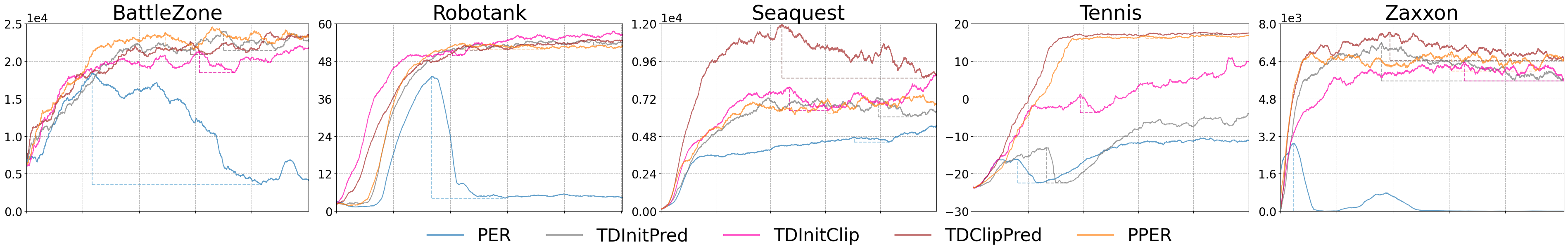
Figure 9: Traing curves of PER, PPER, and the three combinations (TDInitPred, TDInitClip, and TDClipPred). Except TDInitPred in Tennis, all the proposed methods overcome the severe forgetting that PER has experienced in the games.

The following figures show the statistically stable behavior of TDPred. See also Figure 5(d) and related discussions in Section 3.

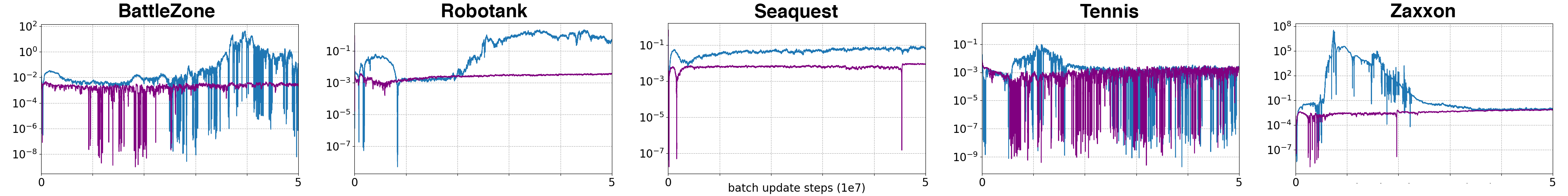
(a) Magnitude of average

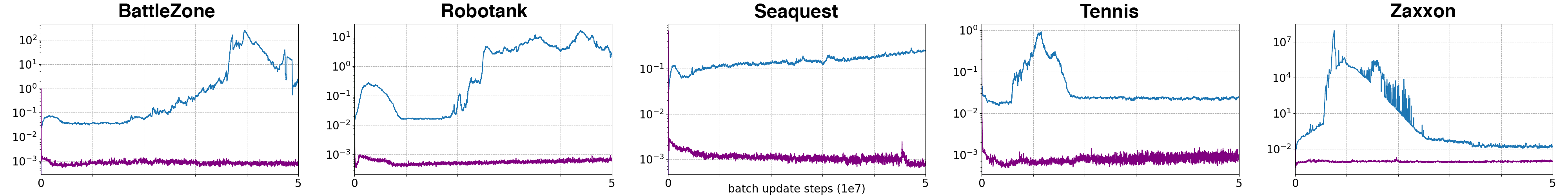
(b) Standard Deviation

Figure 10: Statistics of the batch mean of $\delta$ (PER, blue) and $\hat{\delta}$ (TDPred , violet), up to $T_{\mathsf{max}}=50$M training steps. In the figures, (a) magnitude of average and (b) standard deviation for the TDPred are much stabilized, with (b) much lower variance than PER, showing the stable behavior that can prevents priority explosion.

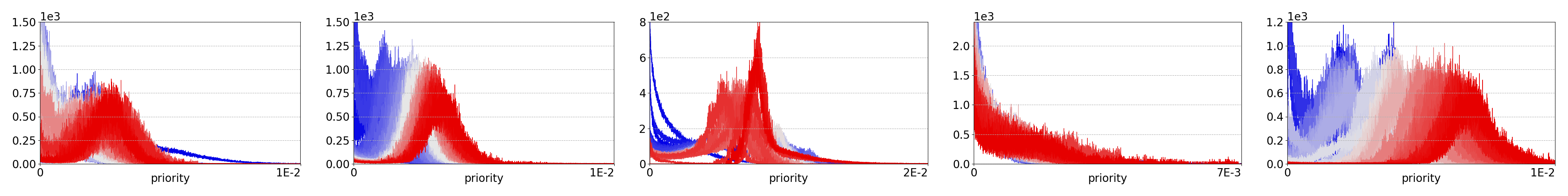
(a) Priority distributions of TDPred

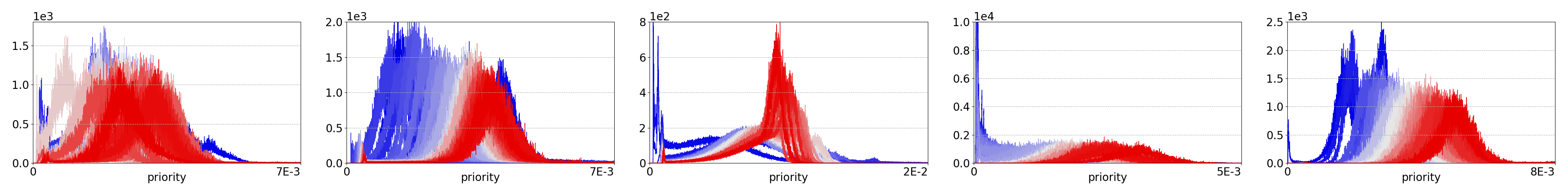
(b) Priority distributions of PPER

Figure 11: Priority distribution changes over the training for 5 Atari games (from left: BattleZone, Robotank, Seaquest, Tennis and Zaxxon). The colors of distributions change from blue to red as the training steps increase up to $T_{\mathsf{max}}=50$M.

Appendix E Training Curves

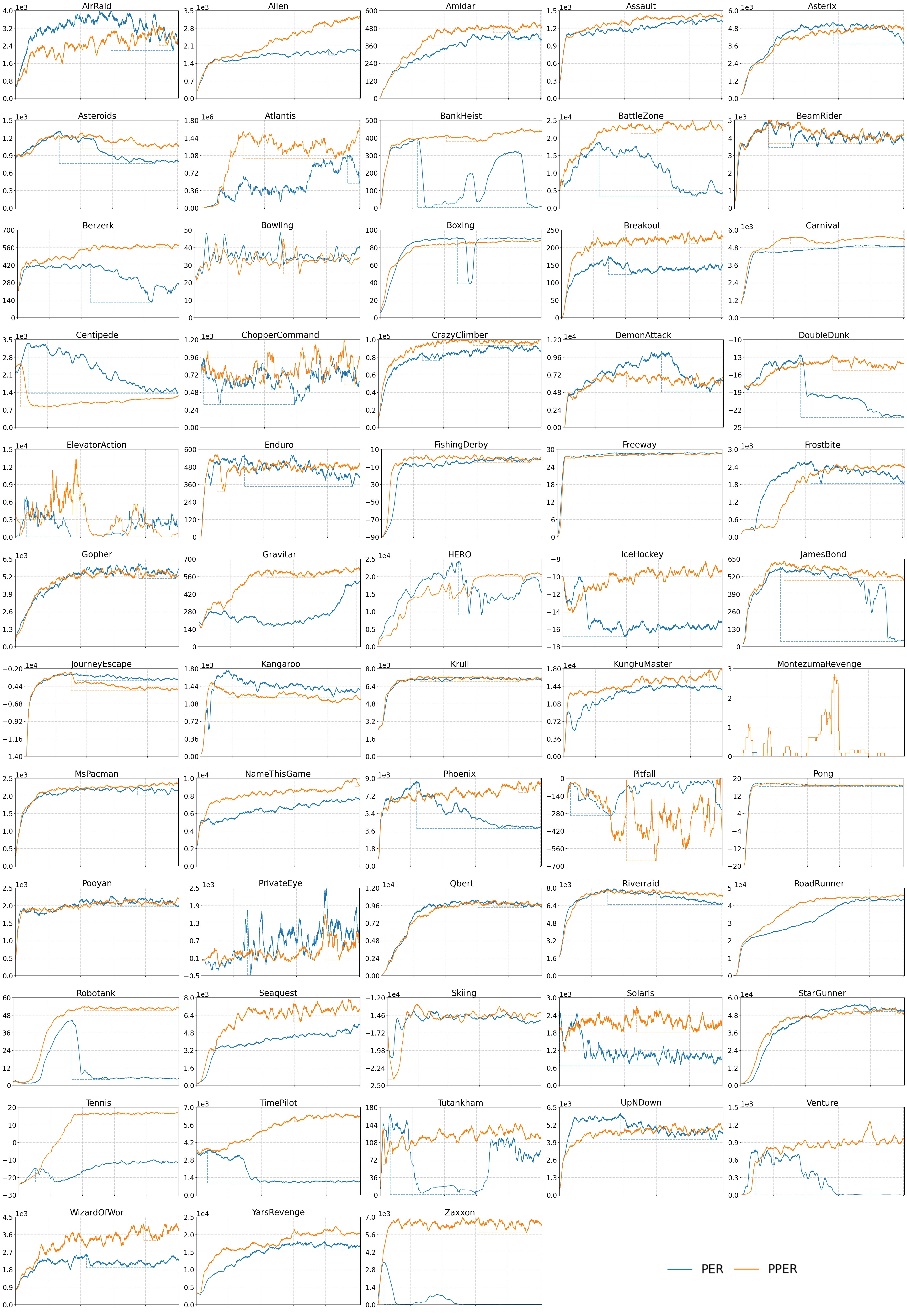
Figure 12: Training curves up to 50 million frames, in raw scores, for 58 games of Atari 2600. In most of the cases, PPER either reaches outperforming performance of PER in the early stage and then tends to be stabilized, or keeps/improves the score steadily over the entire training, with no or less forgetting — showing the stable learning performance of PPER. The vertical dotted line of each learning curve represents $\mathrm{forget}(T^{*})$, the maximum score forget.

Appendix F Raw Test Scores of 58 Atari 2600 Games

Games	Scores				Relative Scores
	Random	Human	PER (50M)	PPER (50M)
AirRaid	-	-	5817.9	6281.8	-
Alien	227.8	7127.7	2220.5	5009.5	40.42
Amidar	5.8	1719.5	573.1	574.1	0.05
Assault	222.4	742.0	3656.0	2371.8	-37.40
Asterix	210.0	8503.3	5904.0	7835.5	23.28
Asteroids	719.1	47388.7	1232.8	1261.5	0.06
Atlantis	12850	29028.1	657339.0	699726.0	6.57
BankHeist	14.2	753.1	712.3	921.8	28.35
BattleZone	2360	37187.5	22110.0	26295.0	12.01
BeamRider	363.9	16926.5	7025.2	6999.3	-0.15
Berzerk	123.7	2630.4	615.8	804.6	7.53
Bowling	23.1	160.7	28.8	25.4	-2.47
Boxing	0.1	12.1	98.0	96.2	-1.83
Breakout	1.7	30.5	356.8	409.4	14.81
Carnival	-	-	5079.4	5624.9	-
Centipede	2090.9	12017.0	3088.7	3416.2	3.29
ChopperCommand	811.0	7387.8	821.0	824.0	0.04
CrazyClimber	10780.5	35829.4	125451.5	119479.5	-5.20
DemonAttack	152.1	1971.0	21292.5	12223.0	-42.90
DoubleDunk	-18.6	16.4	-9.6	-13.5	-11.14
ElevatorAction	-	-	5197.5	6763.0	-
Enduro	0.0	860.5	954.7	1152.0	20.66
FishingDerby	-91.7	-38.7	3.4	-0.3	-3.89
Freeway	0.0	29.6	33.6	33.3	-0.89
Frostbite	65.2	4334.7	2823.2	3396.4	13.42
Gopher	257.6	2412.5	12880.5	8599.4	-33.91
Gravitar	173.0	3351.4	439.0	662.5	7.03
HERO	1027.0	30826.4	25319.6	19555.1	-19.34
IceHockey	-11.2	0.9	-10.0	-7.5	20.66
Jamesbond	29.0	302.8	649.8	676.3	4.26
JourneyEscape	-	-	-1457.5	-1742.5	-
Kangaroo	52.0	3035.0	3434.5	2466.0	-28.63
Krull	1598.0	2665.5	8259.8	8433.6	2.60
KungFuMaster	258.5	22736.3	13632.0	19339.5	25.39
MontezumaRevenge	0.0	4753.3	0.0	0.0	0.00
MsPacman	307.3	6951.6	2131.3	2434.2	4.55
NameThisGame	2292.3	8049.0	9275.0	10293.3	14.58
Phoenix	761.4	7242.6	12035.3	12719.9	6.07
Pitfall	-229.4	6463.7	-1.7	-46.1	-0.66
Pong	-20.7	14.6	20.8	20.7	-0.24
Pooyan	-	-	4116.6	2476.5	-
PrivateEye	24.9	69571.3	0.0	0.5	0.00
Qbert	163.9	13455.0	14804.6	14897.9	0.63
Riverraid	1338.5	17118.0	11045.8	11422.7	2.38
RoadRunner	11.5	7845.0	56092.5	55692.0	-0.71
Robotank	2.2	11.9	44.4	56.6	28.90
Seaquest	68.4	42054.7	6359.5	11055.7	11.18
Skiing	-17098.1	-4336.9	-29974.3	-11665.5	143.40
Solaris	1236.3	12326.7	3899.2	3332.1	-5.11
StarGunner	664.0	10250.0	64750.0	59603.5	-8.03
Tennis	-23.8	-8.3	10.0	21.4	33.72
TimePilot	3568.0	5229.2	3800.0	6557.5	165.90
Tutankham	11.4	167.6	144.2	89.2	-35.21
UpNDown	533.4	11693.2	12493.2	17059.2	38.17
Venture	0.0	1187.5	932.0	1251.5	26.90
WizardOfWor	563.5	4756.5	2286.0	4326.5	48.66
YarsRevenge	3092.9	54576.9	26539.8	30567.5	7.82
Zaxxon	32.5	9173.3	4066.5	8632.5	49.95

Appendix G Experiments on PPER
  with A Smaller Fully-connected Layer of TDPred

Our TDPred architecture is reasonable in the context of following assumptions: 1) it should contain convolutional layers as much as the DQN has, 2) reusing DQN’s convolutional layers is important to establish the common ground of DQN and TDPred (See Section 3.3; Appendix C.2 for details). However, as we introduced in Section 4, the number of neurons $M$ in TDPred’s fully-connected layer is an important hyperparameter of proposed method: it trades off priority and diversity of experience sampling, and also the complexity of algorithm. Here we provide detailed experimental results including test scores.

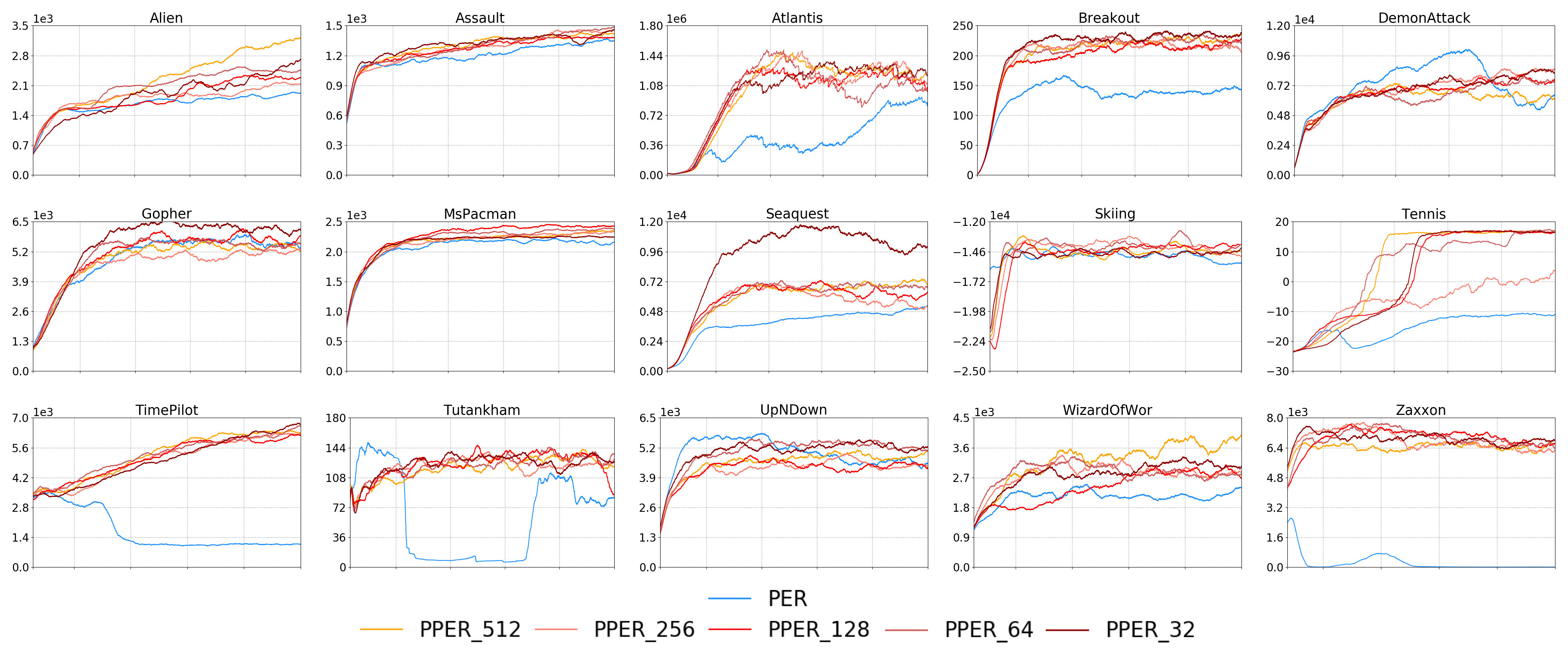
Figure 13: Training curves in raw scores up to 50 million frames of PPER for the number of neurons $M=32,64,128,256,512$ in TDPred’s fully connected layer.

Figure 13 shows training curves of 15 games, for all variations of PPER. We first observe that the ability of PPER—stable and steady learning—is not sensitive to $M$ in most cases. Also there is no general tendency of relation between $M$ and training performance. This is probably because each environment has different characteristic, requiring different balancing of priority and diversity.

We summarized the no-ops start test results in Table 1, where each score is averaged over $200$ repetitions. Based on this experimental result, we hypothesize that the capability of PPN does not significantly affect the effectiveness of the PPER algorithm, possibly the precision of TD-error approximation is less critical in the prioritization scheme, as in rank-based PER (Schaul et al., 2016).

Table 1: Test scores of 15 Atari 2600 games.

Games	Scores
	PER	PPER_512	PPER_256	PPER_128	PPER_64	PPER_32
Alien	2220.5	5009.5	2354.0	2850.6	2786.8	2410.0
Assault	3656.0	2371.8	3995.0	3214.0	3993.2	2927.4
Atlantis	657339.0	699726.0	744829.5	763022.5	753323.5	625574.0
Breakout	356.8	409.4	413.6	235.8	432.9	440.6
DemonAttack	21292.5	12223.0	16835.4	12304.4	15513.5	16937.4
Gopher	12880.5	8599.4	6546.8	11138.4	10587.4	12395.6
MsPacman	2131.3	2434.2	2306.2	2701.5	2694.2	2351.6
Seaquest	6359.5	11055.7	8725.6	11495.8	13061	16210.5
Skiing	-29974.3	-11665.5	-26158.3	-9379.1	-29973.7	-29974.8
Tennis	10.0	21.4	18.0	20.7	21.8	21.8
TimePilot	3800.0	6557.5	6369.5	6277.0	7363.0	6414.5
Tutankham	144.2	89.2	214.8	180.7	117.4	75.5
UpNDown	12493.2	17059.2	6077.1	11480.4	7818.9	7735.9
WizardOfWor	2286.0	4326.5	2566.5	1513.5	3660.0	4081.0
Zaxxon	4066.5	8632.5	9166.5	8526.0	8677.0	8433.0

The computational cost of TDPred’s update dominates the computational overhead of PPER. However, in Table 2 we computed and listed computational costs of the TDPred’s tasks. Updating the TDPred used in experiments adds up about 10.9% of computational cost without GPU usage, which is not a significant increase. This is because TDPred of proposed method is designed to simply reuse the outputs of the convolutional layers of the DQN $Q_{\theta}$ for each frame input $s$ and $s^{\prime}$, since both $\delta$ and $\hat{\delta}$ are computed at the same place in the batch loop of PPER (lines 2–2).

Table 2: Relative computational costs of TDPred’s task, 100% means the cost is equal to DQN’s.

	Computing TD-error ${\hat{\delta}}_{\vartheta}$	Updating the weights $\vartheta$
PPER_512	66.3%	10.9%
PPER_256	62.5%	7.5%
PPER_128	60.9%	6.6%

Another notable fact is that the TDPred can predict TD-errors with approximately 33% less computation: it only requires a single feed-forwarding, while computing the raw TD error for the double DQN bootstrapped target requires feed-forwarding three times.

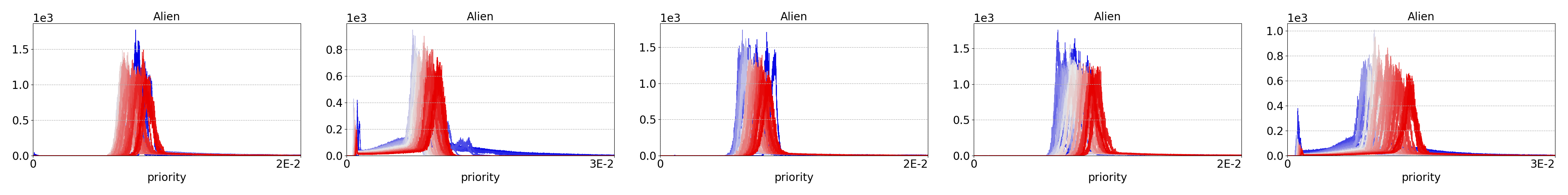
(a) Priority distributions of Alien

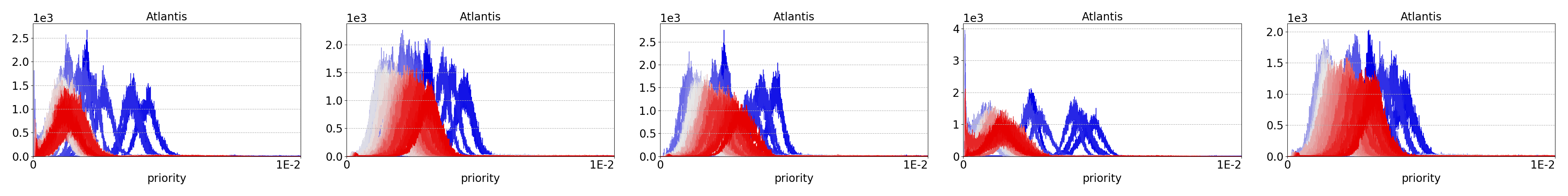
(b) Priority distributions of Atlantis

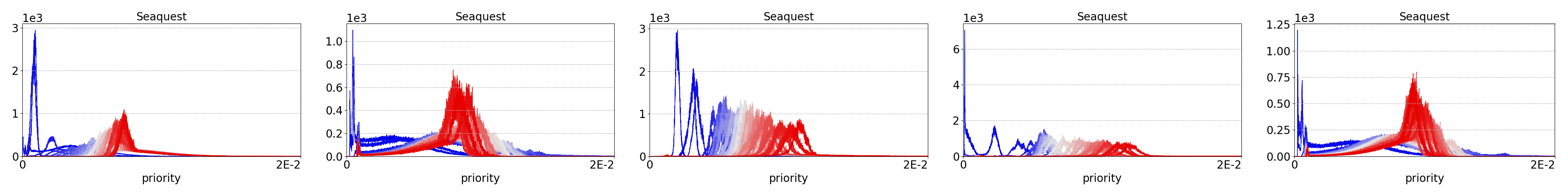
(c) Priority distributions Seaquest

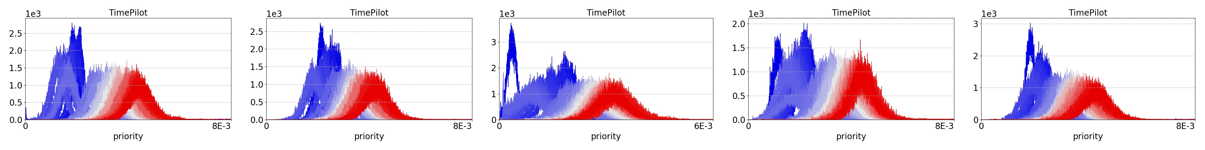
(d) Priority distributions TimePilot

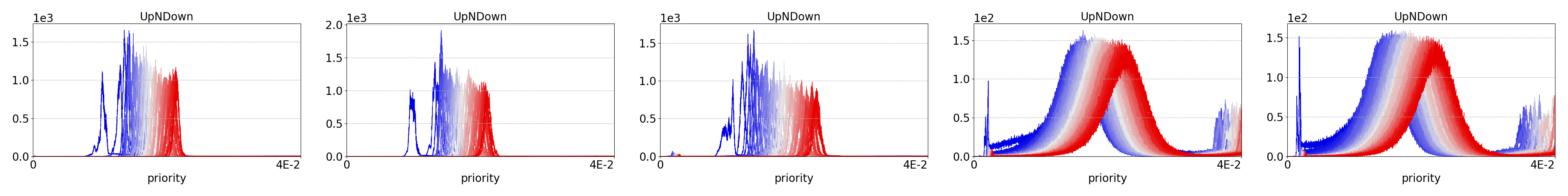
(e) Priority distributions UpNDown

Figure 14: Priority distribution changes over the training for all variations (From left: PPER_32, PPER_64, PPER_128, PPER_256 and PPER_512). The colors of distributions change from blue to red, as the training steps increase up to $T_{\mathsf{max}}=50$M.

Appendix H Statistics of TD-error $\delta$ and TDPred Output $\hat{\delta}$

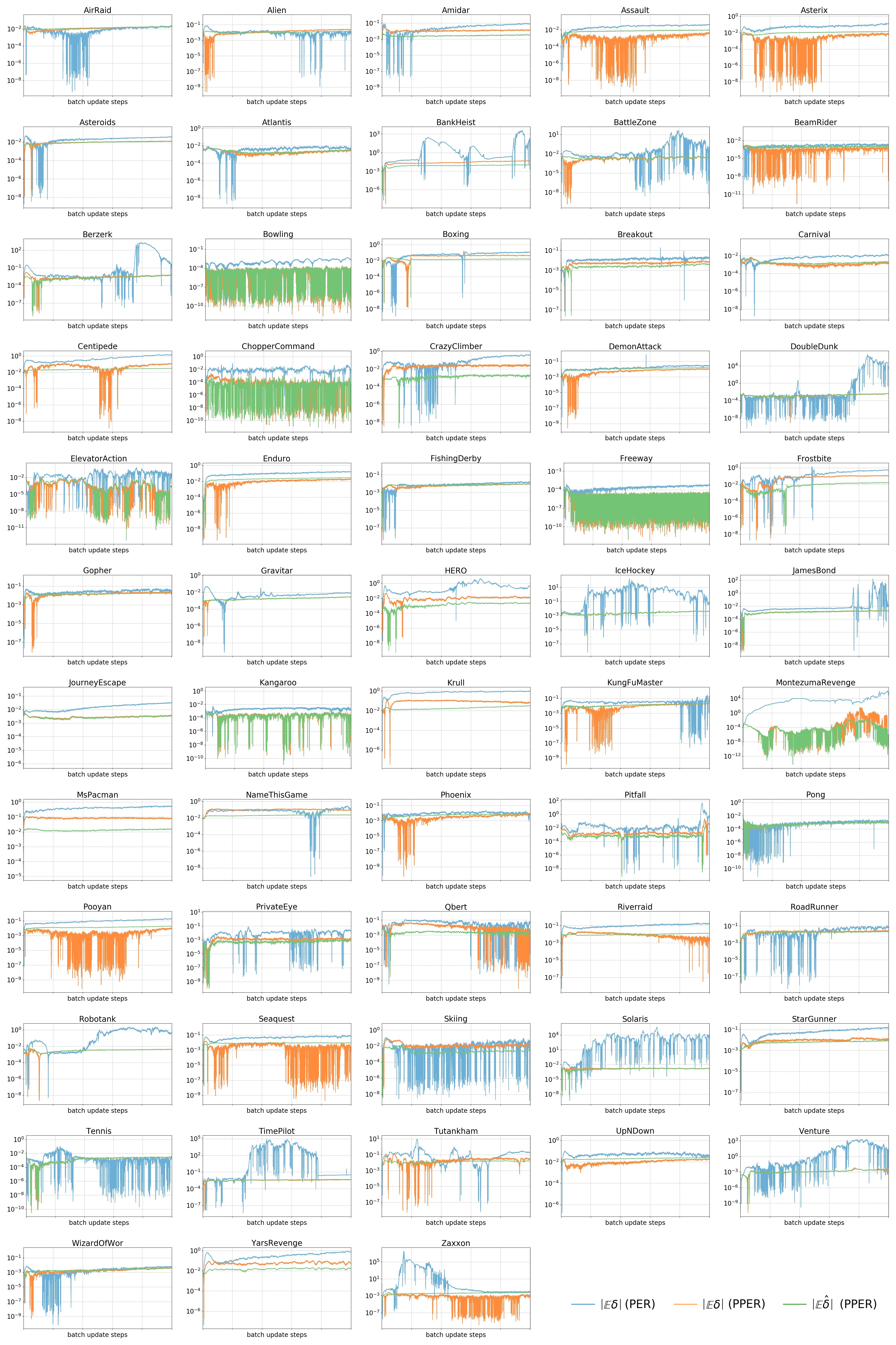
Figure 15: Magnitudes of averages of batch mean $\delta$ (PER, PPER) and ${\hat{\delta}}$ (PPER), over 58 Atari game. Note that (i) the mean of $\hat{\delta}$ (PPER, green) follows that of $\delta$ (PPER, orange) quite accurately, with small biases; (ii) PER (blue) shows huge priority explosions for some cases, while PPER does not.

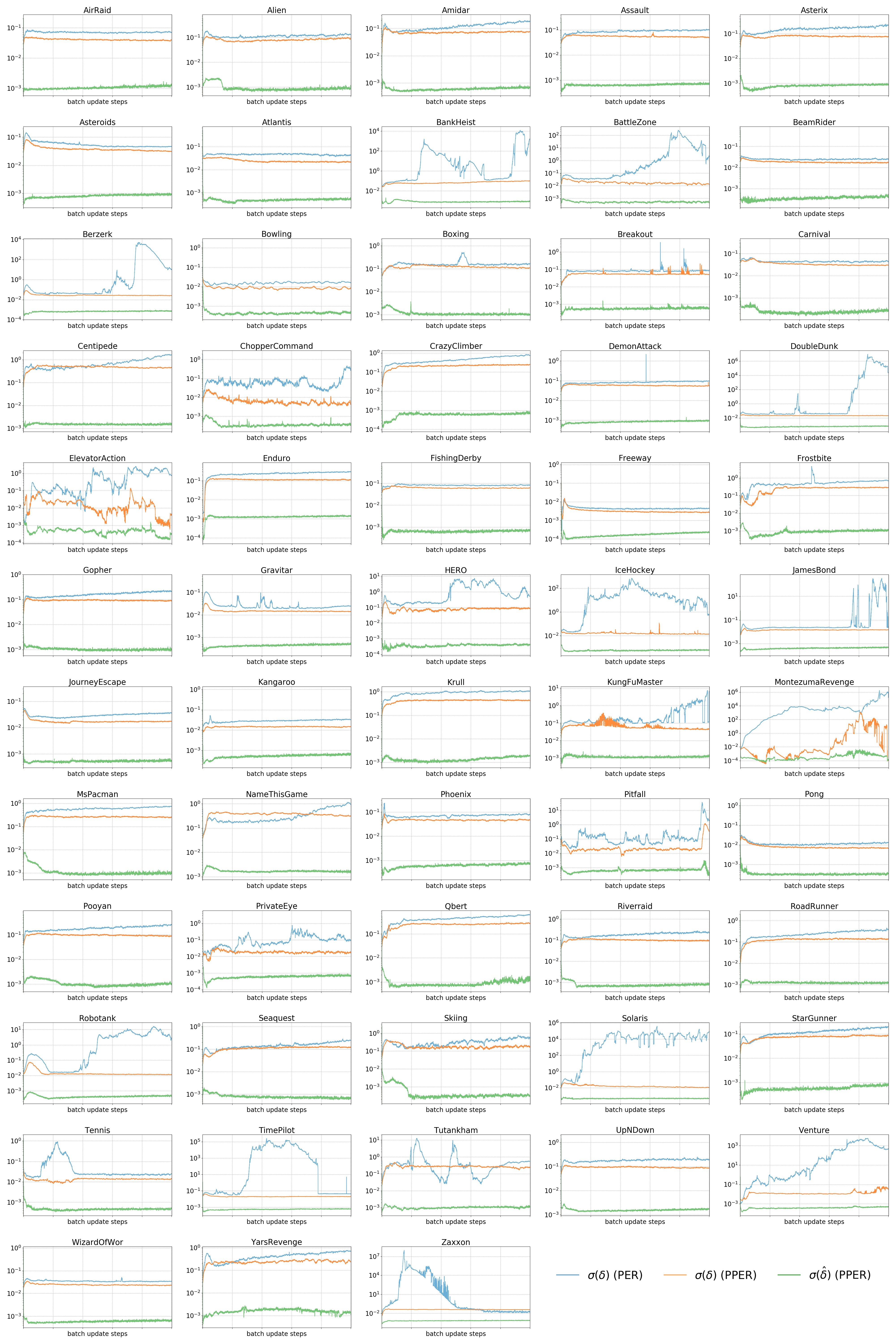
Figure 16: Standard deviations of batch mean $\delta$ (PER, PPER) and ${\hat{\delta}}$ (PPER) over 58 Atari games. Note (i) the reduced standard deviation of $\hat{\delta}$ (PPER, green) and that (ii) the standard deviation of $\delta$ in PPER (orange) is more stabilized than that in PER (blue).

References

- Andre et al. (1998) David Andre, Nir Friedman, and Ronald Parr. Generalized prioritized sweeping. In M. I. Jordan, M. J. Kearns, and S. A. Solla (eds.), Advances in Neural Information Processing Systems 10, pp. 1001–1007. MIT Press, 1998. URL http://papers.nips.cc/paper/1409-generalized-prioritized-sweeping.pdf.
- Andrychowicz et al. (2017) Marcin Andrychowicz, Filip Wolski, Alex Ray, Jonas Schneider, Rachel Fong, Peter Welinder, Bob McGrew, Josh Tobin, OpenAI Pieter Abbeel, and Wojciech Zaremba. Hindsight experience replay. In Advances in neural information processing systems, pp. 5048–5058, 2017.
- Brittain et al. (2019) Marc Brittain, Josh Bertram, Xuxi Yang, and Peng Wei. Prioritized sequence experience replay. arXiv preprint arXiv:1905.12726, 2019.
- de Bruin et al. (2015) Tim de Bruin, Jens Kober, Karl Tuyls, and Robert Babuška. The importance of experience replay database composition in deep reinforcement learning. In Deep reinforcement learning workshop, NIPS, 2015.
- de Bruin et al. (2018) Tim de Bruin, Jens Kober, Karl Tuyls, and Robert Babuška. Experience selection in deep reinforcement learning for control. Journal of Machine Learning Research, 19(9):1–56, 2018. URL http://jmlr.org/papers/v19/17-131.html.
- Geman et al. (1992) Stuart Geman, Elie Bienenstock, and René Doursat. Neural networks and the bias/variance dilemma. Neural computation, 4(1):1–58, 1992.
- Hessel et al. (2018) Matteo Hessel, Joseph Modayil, Hado Van Hasselt, Tom Schaul, Georg Ostrovski, Will Dabney, Dan Horgan, Bilal Piot, Mohammad Azar, and David Silver. Rainbow: Combining improvements in deep reinforcement learning. In Thirty-Second AAAI Conference on Artificial Intelligence, 2018.
- Hester et al. (2018) Todd Hester, Matej Vecerik, Olivier Pietquin, Marc Lanctot, Tom Schaul, Bilal Piot, Dan Horgan, John Quan, Andrew Sendonaris, Ian Osband, et al. Deep q-learning from demonstrations. In Thirty-Second AAAI Conference on Artificial Intelligence, 2018.
- Horgan et al. (2018) Dan Horgan, John Quan, David Budden, Gabriel Barth-Maron, Matteo Hessel, Hado van Hasselt, and David Silver. Distributed prioritized experience replay. In International Conference on Learning Representations, 2018. URL https://openreview.net/forum?id=H1Dy---0Z.
- Hou et al. (2017) Yuenan Hou, Lifeng Liu, Qing Wei, Xudong Xu, and Chunlin Chen. A novel ddpg method with prioritized experience replay. In 2017 IEEE International Conference on Systems, Man, and Cybernetics (SMC), pp. 316–321. IEEE, 2017.
- Lillicrap et al. (2015) Timothy P Lillicrap, Jonathan J Hunt, Alexander Pritzel, Nicolas Heess, Tom Erez, Yuval Tassa, David Silver, and Daan Wierstra. Continuous control with deep reinforcement learning. arXiv preprint arXiv:1509.02971, 2015.
- Lin (1992) Long-Ji Lin. Self-improving reactive agents based on reinforcement learning, planning and teaching. Machine learning, 8(3-4):293–321, 1992.
- Mahmood et al. (2014) A Rupam Mahmood, Hado P van Hasselt, and Richard S Sutton. Weighted importance sampling for off-policy learning with linear function approximation. In Advances in Neural Information Processing Systems, pp. 3014–3022, 2014.
- Matthews et al. (2018) Alexander G de G Matthews, Mark Rowland, Jiri Hron, Richard E Turner, and Zoubin Ghahramani. Gaussian process behaviour in wide deep neural networks. arXiv preprint arXiv:1804.11271, 2018.
- Mnih et al. (2013) Volodymyr Mnih, Koray Kavukcuoglu, David Silver, Alex Graves, Ioannis Antonoglou, Daan Wierstra, and Martin Riedmiller. Playing atari with deep reinforcement learning. arXiv preprint arXiv:1312.5602, 2013.
- Mnih et al. (2015) Volodymyr Mnih, Koray Kavukcuoglu, David Silver, Andrei A Rusu, Joel Veness, Marc G Bellemare, Alex Graves, Martin Riedmiller, Andreas K Fidjeland, Georg Ostrovski, et al. Human-level control through deep reinforcement learning. Nature, 518(7540):529–533, 2015.
- Moore & Atkeson (1993) Andrew W Moore and Christopher G Atkeson. Prioritized sweeping: Reinforcement learning with less data and less time. Machine learning, 13(1):103–130, 1993.
- Nair et al. (2015) Arun Nair, Praveen Srinivasan, Sam Blackwell, Cagdas Alcicek, Rory Fearon, Alessandro De Maria, Vedavyas Panneershelvam, Mustafa Suleyman, Charles Beattie, Stig Petersen, et al. Massively parallel methods for deep reinforcement learning. arXiv preprint arXiv:1507.04296, 2015.
- Neal et al. (2018) Brady Neal, Sarthak Mittal, Aristide Baratin, Vinayak Tantia, Matthew Scicluna, Simon Lacoste-Julien, and Ioannis Mitliagkas. A modern take on the bias-variance tradeoff in neural networks. arXiv preprint arXiv:1810.08591, 2018.
- Pan et al. (2018) Yangchen Pan, Muhammad Zaheer, Adam White, Andrew Patterson, and Martha White. Organizing experience: a deeper look at replay mechanisms for sample-based planning in continuous state domains. arXiv preprint arXiv:1806.04624, 2018.
- Schaul et al. (2016) Tom Schaul, John Quan, Ioannis Antonoglou, and David Silver. Prioritized experience replay. In Yoshua Bengio and Yann LeCun (eds.), 4th International Conference on Learning Representations, ICLR 2016, San Juan, Puerto Rico, May 2-4, 2016, Conference Track Proceedings, 2016. URL http://arxiv.org/abs/1511.05952.
- Silver et al. (2017) David Silver, Julian Schrittwieser, Karen Simonyan, Ioannis Antonoglou, Aja Huang, Arthur Guez, Thomas Hubert, Lucas Baker, Matthew Lai, Adrian Bolton, et al. Mastering the game of go without human knowledge. Nature, 550(7676):354–359, 2017.
- Sutton & Barto (2018) R. S. Sutton and A. G. Barto. Reinforcement learning: an introduction. Second Edition, MIT Press, Cambridge, MA (available at http://incompleteideas.net/book/the-book.html), 2018.
- Van Hasselt et al. (2016) Hado Van Hasselt, Arthur Guez, and David Silver. Deep reinforcement learning with double q-learning. In Thirtieth AAAI conference on artificial intelligence, 2016.
- van Seijen & Sutton (2015) Harm van Seijen and Rich Sutton. A deeper look at planning as learning from replay. In International conference on machine learning, pp. 2314–2322, 2015.
- Vecerik et al. (2017) Mel Vecerik, Todd Hester, Jonathan Scholz, Fumin Wang, Olivier Pietquin, Bilal Piot, Nicolas Heess, Thomas Rothörl, Thomas Lampe, and Martin Riedmiller. Leveraging demonstrations for deep reinforcement learning on robotics problems with sparse rewards. arXiv preprint arXiv:1707.08817, 2017.
- Wang et al. (2015) Ziyu Wang, Tom Schaul, Matteo Hessel, Hado Van Hasselt, Marc Lanctot, and Nando De Freitas. Dueling network architectures for deep reinforcement learning. arXiv preprint arXiv:1511.06581, 2015.
- Wang et al. (2016) Ziyu Wang, Victor Bapst, Nicolas Heess, Volodymyr Mnih, Remi Munos, Koray Kavukcuoglu, and Nando de Freitas. Sample efficient actor-critic with experience replay. arXiv preprint arXiv:1611.01224, 2016.
- Zha et al. (2019) Daochen Zha, Kwei-Herng Lai, Kaixiong Zhou, and Xia Hu. Experience replay optimization. In Proceedings of the 28th International Joint Conference on Artificial Intelligence, pp. 4243–4249. AAAI Press, 2019.
- Zhang & Sutton (2017) Shangtong Zhang and Richard S Sutton. A deeper look at experience replay. arXiv preprint arXiv:1712.01275, 2017.
- Zhao & Tresp (2019) Rui Zhao and Volker Tresp. Curiosity-driven experience prioritization via density estimation. arXiv preprint arXiv:1902.08039, 2019.