Fast and Accurate Anomaly Detection in Dynamic Graphs
with a Two-Pronged Approach

Abstract.

Given a dynamic graph stream, how can we detect the sudden appearance of anomalous patterns, such as link spam, follower boosting, or denial of service attacks? Additionally, can we categorize the types of anomalies that occur in practice, and theoretically analyze the anomalous signs arising from each type?

In this work, we propose AnomRank, an online algorithm for anomaly detection in dynamic graphs. AnomRank uses a two-pronged approach defining two novel metrics for anomalousness. Each metric tracks the derivatives of its own version of a ‘node score’ (or node importance) function. This allows us to detect sudden changes in the importance of any node. We show theoretically and experimentally that the two-pronged approach successfully detects two common types of anomalies: sudden weight changes along an edge, and sudden structural changes to the graph. AnomRank is (a) Fast and Accurate: up to 49.5$\times$ faster or 35% more accurate than state-of-the-art methods, (b) Scalable: linear in the number of edges in the input graph, processing millions of edges within 2 seconds on a stock laptop/desktop, and (c) Theoretically Sound: providing theoretical guarantees of the two-pronged approach.

1. Introduction

Network-based systems including computer networks and social network services have been a focus of various attacks. In computer networks, distributed denial of service (DDOS) attacks use a number of machines to make connections to a target machine to block their availability. In social networks, users pay spammers to ”Like” or ”Follow” their page to manipulate their public trust. By abstracting those networks to a graph, we can detect those attacks by finding suddenly emerging anomalous signs in the graph.

Various approaches have been proposed to detect anomalies in graphs, the majority of which focus on static graphs (Akoglu et al., 2010; Chakrabarti, 2004; Hooi et al., 2017; Jiang et al., 2016; Kleinberg, 1999; Shin et al., 2018a; Tong and Lin, 2011). However, many real-world graphs are dynamic, with timestamps indicating the time when each edge was inserted/deleted. Static anomaly detection methods, which are solely based on static connections, miss useful temporal signals of anomalies.

Several approaches (Eswaran et al., 2018; Shin et al., 2017; Eswaran and Faloutsos, 2018) have been proposed to detect anomalies on dynamic graphs (we review these in greater detail in Section 2 and Table 1). However, they are not satisfactory in terms of accuracy and speed. Accurately detecting anomalies in near real-time is important in order to cut back the impact of malicious activities and start recovery processes in a timely manner.

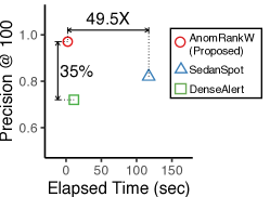
(a) Speed and precision of AnomRank

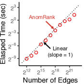
(b) Scalability of AnomRank

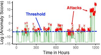
(c) Effectiveness of AnomRank

Figure 1. AnomRank is accurate, fast, and scalable: (a) Precision at top-100 and running time on the DARPA dataset: AnomRank is significantly faster than state-of-the-art methods while achieving higher accuracy. (b) AnomRank scales linearly with the number of edges in the input dynamic graph. (c) AnomRank computes anomaly scores (green line) on the DARPA dataset. Red crosses indicate ground truth anomalies; the blue line is an anomalousness threshold. $77$% of green spikes above the blue line are true positives; see Section 5 for details.

In this paper, we propose AnomRank, a fast and accurate online algorithm for detecting anomalies in dynamic graphs with a two-pronged approach. We classify anomalies in dynamic graphs into two types: AnomalyS and AnomalyW. AnomalyS denotes suspicious changes to the structure of the graph, such as through the addition of edges between previously unrelated nodes in spam attacks. AnomalyW indicates anomalous changes in the weight (i.e. number of edges) between connected nodes, such as suspiciously frequent connections in port scan attacks.

Various node score functions have been proposed to map each node of a graph to an importance score: PageRank (Page et al., 1999), HITS and its derivatives (SALSA) (Kleinberg, 1999; Lempel and Moran, 2001), Fiedler vector (Chung, 1994), etc. Our intuition is that anomalies induce sudden changes in node scores. Based on this intuition, AnomRank focuses on the 1st and 2nd order derivatives of node scores to detect anomalies with large changes in node scores within a short time. To detect AnomalyS and AnomalyW effectively, we design two versions of node score functions based on characteristics of these two types of anomalies. Then, we define two novel metrics, AnomRankS and AnomRankW, which measure the 1st and 2nd order derivatives of our two versions of node score functions, as a barometer of anomalousness. We theoretically analyze the effectiveness of each metric on the corresponding anomaly type, and provide rigid guarantees on the accuracy of AnomRank. Through extensive experiments with real-world and synthetic graphs, we demonstrate the superior performance of AnomRank over existing methods. Our main contributions are:

• Online, two-pronged approach: We introduce AnomRank, an online detection method, for two types of anomalies (AnomalyS, AnomalyW) in dynamic graphs.

• Theoretical guarantees: We prove the effectiveness of our proposed metrics, AnomRankS and AnomRankW, theoretically (Theorems 1 and 2).

• Practicality: Experiments on public benchmarks show that AnomRank outperforms state-of-the-art competitors, being up to $49.5\times$ faster or $35\%$ more accurate (Figure 1). Moreover, thanks to its two-pronged approach, it spots anomalies that the competitors miss (Figure 4).

Reproducibility: our code and data are publicly available. The paper is organized in the usual way (related work, preliminaries, proposed method, experiments, and conclusions).

2. Related Work

We discuss previous work on detecting anomalous entities (nodes, edges, events, etc.) on static and dynamic graphs. See (Akoglu et al., 2015) for an extensive survey on graph-based anomaly detection.

Anomaly detection in static graphs can be described under the following categories:

• Anomalous Node Detection: (Akoglu et al., 2010) extracts egonet-based features and finds empirical patterns with respect to the features. Then, it identifies nodes whose egonets deviate from the patterns. (Xu et al., 2007) groups nodes that share many neighbors and spots nodes that cannot be assigned to any community.

• Anomalous Edge Detection: (Chakrabarti, 2004) encodes the input graph based on similar connectivity between nodes, then spots edges whose removal significantly reduces the total encoding cost. (Tong and Lin, 2011) factorizes the adjacency matrix and flags edges which introduce high reconstruction error as outliers.

• Anomalous Subgraph Detection: (Hooi et al., 2017) and (Shin et al., 2018a) measure the anomalousness of nodes and edges, then find a dense subgraph consisting of many anomalous nodes and edges.

Anomaly detection in dynamic graphs can also be described under the following categories:

• Anomalous Node Detection: (Sun et al., 2006) approximates the adjacency matrix of the current snapshot based on incremental matrix factorization. Then, it spots nodes corresponding to rows with high reconstruction error. (Wang et al., 2015) computes nodes features (degree, closeness centrality, etc) in each graph snapshot. Then, it identifies nodes whose features are notably different from their previous values and the features of nodes in the same community.

• Anomalous Edge Detection: (Eswaran and Faloutsos, 2018) detects edges that connect sparsely-connected parts of a graph. (Ranshous et al., 2016) spots edge anomalies based on their occurrence, preferential attachment and mutual neighbors.

• Anomalous Subgraph Detection: (Beutel et al., 2013) spots near-bipartite cores where each node is connected to others in the same core densly within a short time. (Jiang et al., 2016) and (Shin et al., 2018b) detect groups of nodes who form dense subgraphs in a temporally synchronized manner. (Shin et al., 2017) identifies dense subtensors created within a short time.

• Event Detection: (Eswaran et al., 2018; Aggarwal et al., 2011; Koutra et al., 2016; Henderson et al., 2010) detect the following events: sudden appearance of many unexpected edges (Aggarwal et al., 2011), sudden appearance of a dense graph (Eswaran et al., 2018), sudden drop in the similarity between two consecutive snapshots (Koutra et al., 2016), and sudden prolonged spikes and lightweight stars (Henderson et al., 2010).

Our proposed AnomRank is an anomalous event detection method with fast speed and high accuracy. It can be easily extended to localize culprits of anomalies into nodes and substructures (Section 4.4), and it detects various types of anomalies in dynamic graphs in a real-time. Table 1 compares AnomRank to existing methods.

Table 1. AnomRank out-features competitors: comparison of our proposed AnomRank and existing methods for anomaly detection in dynamic graphs.

	Oddball (Akoglu et al., 2010)	MetricFor. (Henderson et al., 2010)	CC, CS(Beutel et al., 2013; Jiang et al., 2016)	DenseAlert (Shin et al., 2017)	SpotLight (Eswaran et al., 2018)	SedanSpot (Eswaran and Faloutsos, 2018)	AnomRank
Real-time detection∗				✓			✓
Allow edge deletions				✓	✓		✓
Structural anomalies	✓	✓					✓
Edge weight anomalies	✓	✓	✓	✓	✓	✓	✓

• ^∗compute $1$M edges within $5$ seconds.

3. Preliminaries

Table 2 gives a list of symbols and definitions.

Various node score functions have been designed to estimate importance (centrality, etc.) of nodes in a graph: PageRank (Page et al., 1999); HITS (Kleinberg, 1999) and its derivatives (SALSA) (Lempel and Moran, 2001); Fiedler vector (Chung, 1994); all the centrality measures from social network analysis (eigenvector-, degree-, betweeness-centrality (Wasserman and Faust, 1994)). Among them, we extend PageRank to design our node score functions in Section 4.2 because (a) it is fast to compute, (b) it led to the ultra-successful ranking method of Google, (c) it is intuitive (‘your importance depends on the importance of your neighbors’). Next, we briefly review PageRank and its incremental version in dynamic graphs.

PageRank

As shown in (Yoon et al., 2018b), PageRank scores for all nodes are represented as a PageRank score vector $\mathbf{p}$ which is defined by the following equation:

$$\mathbf{p}=(1-c)\sum_{i=0}^{\infty}(c\mathbf{\tilde{A}}^{\top})^{i}\mathbf{b}$$

where $c$ is a damping factor, $\mathbf{\tilde{A}}$ is the row-normalized adjacency matrix, and $\mathbf{b}$ is the starting vector. This equation is interpreted as a propagation of scores across a graph: initial scores in the starting vector $\mathbf{b}$ are propagated across the graph by multiplying with $\mathbf{\tilde{A}}^{\top}$; since the damping factor $c$ is smaller than $1$, propagated scores converge, resulting in PageRank scores. As shown in (Yoon et al., 2018a), PageRank computation time is proportional to the L1 length of the starting vector $\mathbf{b}$, since small L1 length of $\mathbf{b}$ leads to faster convergence of iteration ($\sum_{i=0}^{\infty}(c\mathbf{\tilde{A}}^{\top})^{i}$) with damping factor $c$. Here L1 length of a vector is defined as the sum of absolute values of its entries. The L1 length of a matrix is defined as the maximum L1 length of its columns.

Incremental PageRank

When edges are inserted or deleted, PageRank scores can be updated incrementally from the previous PageRank scores. Let $\mathbf{\tilde{A}}$ be the row-normalized adjacency matrix of a graph $G$ and $\mathbf{\tilde{B}}$ be the row-normalized adjacency matrix after a change $\Delta G$ happened during $\Delta t$. From now on, denote $\Delta\mathbf{A}=\mathbf{\tilde{B}}^{\top}-\mathbf{\tilde{A}}^{\top}$, the difference between transpose of normalized matrices $\mathbf{\tilde{A}}^{\top}$ and $\mathbf{\tilde{B}}^{\top}$.

Lemma 1 (Dynamic PageRank, Theorem 3.2 in (Yoon et al., 2018a)).

Given updates $\Delta\mathbf{A}$ in a graph during $\Delta t$, an updated PageRank vector $\mathbf{p}(t+\Delta t)$ is computed incrementally from a previous PageRank vector $\mathbf{p}(t)$ as follows:

$$\mathbf{p}(t+\Delta t)=\mathbf{p}(t)+\sum_{k=0}^{\infty}(c(\mathbf{\tilde{A}}^{\top}+\Delta\mathbf{A}))^{k}c\Delta\mathbf{A}\mathbf{p}(t)$$

Note that, for small changes in a graph, the L1 length of the starting vector $c\Delta\mathbf{A}\mathbf{p}(t)$ is much smaller than $1$, the L1 length of the starting vector $\mathbf{b}$ in the static PageRank equation, resulting in much faster convergence.

Table 2. Table of symbols.

Symbol	Definition
$G$	(un)directed and (un)weighted input graph
$\Delta G$	update in graph
$n,m$	numbers of nodes and edges in $G$
$\mathbf{\tilde{A}}$	($n\times n$) row-normalized adjacency matrix of $G$
$\mathbf{\tilde{B}}$	($n\times n$) row-normalized adjacency matrix of $G+\Delta G$
$\Delta\mathbf{A}$	($n\times n$) difference between $\mathbf{\tilde{A}}^{\top}$ and $\mathbf{\tilde{B}}^{\top}$ ($=\mathbf{\tilde{B}}^{\top}-\mathbf{\tilde{A}}^{\top}$)
$c$	damping factor of PageRank
$\mathbf{b}_{s}$	($n\times 1$) uniform starting vector
$\mathbf{b}_{w}$	($n\times 1$) out-edge proportional starting vector
$\mathbf{\tilde{A}}_{s}$	($n\times n$) row-normalized unweighted adjacency matrix
$\mathbf{\tilde{A}}_{w}$	($n\times n$) row-normalized weighted adjacency matrix

4. Proposed Method

Node scores present the importance of nodes across a given graph. Thus, as the graph evolves under normal behavior with the insertion and deletion of edges, node scores evolve smoothly. In contrast, anomalies such as network attacks or rating manipulation often aim to complete their goals in a short time, e.g. to satisfy their clients, inducing large and abrupt changes in node scores. Our key intuition is that such abrupt gains or losses are reflected in the 1st and 2nd derivative of node scores: large 1st derivative identifies large changes, while large 2nd derivative identifies abrupt changes in the trend of the data, thereby distinguishing changes from normal users who evolve according to smooth trends. Thus, tracking 1st and 2nd order derivatives helps detect anomalies in dynamic graphs.

Changes in a dynamic graph are classified into two types: structure changes and edge weight changes. Since these two types of changes affect node scores of the graph differently (more details in Section 4.2), we need to handle them separately. Thus, first, we classify anomalies in dynamic graphs into two types: AnomalyS and AnomalyW (Section 4.1). Then we design two node score functions based on characteristics of these two types of anomalies, respectively (Section 4.2). Next, we define two novel metrics for anomalousness using 1st and 2nd order derivatives of our node scores, and verify the effectiveness of each metric on the respective type of anomalies theoretically (Section 4.3). Based on these analyses, we introduce our method AnomRank, a fast and accurate anomaly detection algorithm in dynamic graphs (Section 4.4).

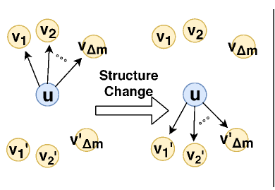
(a) Structure Change

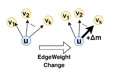
(b) Edge Weight Change

Figure 2. Two-pronged approach: Changes in dynamic graphs are classified into two types, structure change and edge weight change.

4.1. Anomalies in Dynamic Graphs

We classify anomalies in dynamic graphs into two types: AnomalyS and AnomalyW.

4.1.1. AnomalyS

It is suspicious if a number of edges are inserted/deleted among nodes which are previously unrelated/related. Hence, AnomalyS denotes a massive change with regard to the graph structure. One example of AnomalyS is spam in mail network graphs: a spammer sends mail to many unknown individuals, generating out-edges toward previously unrelated nodes. Data exfiltration attacks in computer network graphs are another example: attackers transfer a target’s data stealthily, generating unseen edges around a target machine to steal information. As illustrated in Figure 2, we define a structure change as follows:

Definition 1 (Structure Change).

If a node $u$ changes the destination of $\Delta m$ of its out-edges from previous neighbors $v_{1},\dots,v_{\Delta m}$ to new neighbors $v_{1}^{\prime},\dots,v_{\Delta m}^{\prime}$, we call the change a structure change of size $\Delta m$.

With abnormally large $\Delta m$, a structure change becomes an AnomalyS. To detect AnomalyS, we need to focus on the existence of edges between two nodes, rather than the number of occurrences of edges between two nodes.

4.1.2. AnomalyW

In dynamic graphs, an edge between two nodes could occur several times. Edge weight is proportional to the number of edge occurrences. AnomalyW denotes a massive change of edge weights in a graph. One example of AnomalyW is port scan attacks in computer network graphs: to scan ports in a target IP address, attackers repeatedly connect to the IP address, thus increasing the number of edge occurrences to the target node. On Twitter, high edge density on a user-keyword graph could indicate bot-like behavior, e.g. bots posting about the same content repeatedly. As illustrated in Figure 2, we define an edge weight change as follows:

Definition 2 (Edge Weight Change).

If a node $u$ adds/subtracts $\Delta m$ out-edges to neighbor node $v$, we call the change an edge weight change of size $\Delta m$.

With abnormally large $\Delta m$, an edge weight change becomes an AnomalyW. In contrast to AnomalyS, here we focus on the number of occurrences of each edge, rather than only the presence or absence of an edge.

4.2. Node Score Functions for Detecting AnomalyS and AnomalyW

To detect AnomalyS and AnomalyW, we first define two node score functions, ScoreS and ScoreW, which we use to define our anomalousness metrics in Section 4.3.

4.2.1. ScoreS

We introduce node score ScoreS, which we use to catch AnomalyS. Define the row-normalized unweighted adjacency matrix $\mathbf{\tilde{A}}_{s}$, a starting vector $\mathbf{b}_{s}$ which is an all-$\frac{1}{n}$ vector of length $n$ (the number of nodes), and the damping factor $c$.

Definition 3 (ScoreS).

ScoreS node score vector $\mathbf{p}_{s}$ is defined by the following iterative equation:

$$\mathbf{p}_{s}=c\mathbf{\tilde{A}}_{s}^{\top}\mathbf{p}_{s}+(1-c)\mathbf{b}_{s}$$

For this (unweighted) case, ScoreS is the same as PageRank, but we refer to it as ScoreS for consistency with our later definitions. Note that the number of edge occurrences between nodes is not considered in ScoreS. Using Lemma 1, we can compute ScoreS incrementally at fast speed, in dynamic graphs.

4.2.2. ScoreW

Next, we introduce the second node score, ScoreW, which we use to catch AnomalyW. To incorporate edge weight, we use the weighted adjacency matrix $\mathbf{A}_{w}$ instead of $\mathbf{A}_{s}$. However, this is not enough on its own: imagine an attacker node who adds a massive number of edges, all toward a single target node, and the attacker has no other neighbors. Since $\mathbf{\tilde{A}}_{w}$ is row-normalized, this attacker appears no different in $\mathbf{\tilde{A}}_{w}$ as if they only added a single edge toward the same target. Hence, to catch such attackers, we also introduce an out-degree proportional starting vector $\mathbf{b}_{w}$, i.e. setting the initial scores of each node proportional to its outdegree.

Definition 4 (ScoreW).

ScoreW node score vector $\mathbf{p}_{w}$ is defined by the following iterative equation:

$$\mathbf{p}_{w}=c\mathbf{\tilde{A}}_{w}^{\top}\mathbf{p}_{w}+(1-c)\mathbf{b}_{w}$$

$\mathbf{A}_{w}(i,j)$ is the edge weight from node $i$ to node $j$. $\mathbf{b}_{w}(i)$ is $\frac{m_{i}}{m}$, where $m_{i}$ denotes the total edge weight of out-edges of node $i$, and $m$ denotes the total edge weight of the graph.

Next, we show how ScoreW is computed incrementally in a dynamic graph. Assume that a change $\Delta G$ happens in graph $G$ in time interval $\Delta t$, inducing changes $\Delta\mathbf{A}_{w}$ and $\Delta\mathbf{b}_{w}$ in the adjacency matrix and the starting vector, respectively.

Lemma 2 (Dynamic ScoreW).

Given updates $\Delta\mathbf{A}_{w}$ and $\Delta\mathbf{b}_{w}$ in a graph during $\Delta t$, an updated score vector $\mathbf{p}_{w}(t+\Delta t)$ is computed incrementally from a previous score vector $\mathbf{p}_{w}(t)$ as follows:

$$\mathbf{p}_{w}(t+\Delta t)=~{} \mathbf{p}_{w}(t)+\sum_{k=0}^{\infty}(c(\mathbf{\tilde{A}}_{w}^{\top}+\Delta\mathbf{A}_{w}))^{k}c\Delta\mathbf{A}_{w}\mathbf{p}_{w}(t)$$

$$+(1-c)\sum_{k=0}^{\infty}(c(\mathbf{\tilde{A}}_{w}^{\top}+\Delta\mathbf{A}_{w}))^{k}\Delta\mathbf{b}_{w}$$

Proof.

For brevity, $\mathbf{p}_{w}^{n}\leftarrow\mathbf{p}_{w}(t+\Delta t)$ and $\mathbf{p}_{w}^{o}\leftarrow\mathbf{p}_{w}(t)$.

$$\mathbf{p}_{w}^{n}=(1-c)\sum_{k=0}^{\infty}c^{k}(\mathbf{\tilde{A}}_{w}^{\top}+\Delta\mathbf{A}_{w})^{k}(\mathbf{b}_{w}+\Delta\mathbf{b}_{w})$$

$$=(1-c)\sum_{k=0}^{\infty}c^{k}(\mathbf{\tilde{A}}_{w}^{\top}+\Delta\mathbf{A}_{w})^{k}\mathbf{b}_{w}+(1-c)\sum_{k=0}^{\infty}c^{k}(\mathbf{\tilde{A}}_{w}^{\top}+\Delta\mathbf{A}_{w})^{k}\Delta\mathbf{b}_{w}$$

$$=\mathbf{p}_{w}^{o}+\sum_{k=0}^{\infty}(c(\mathbf{\tilde{A}}_{w}^{\top}+\Delta\mathbf{A}_{w}))^{k}c\Delta\mathbf{A}_{w}\mathbf{p}_{w}^{o}+(1-c)\sum_{k=0}^{\infty}(c(\mathbf{\tilde{A}}_{w}^{\top}+\Delta\mathbf{A}_{w}))^{k}\Delta\mathbf{b}_{w}$$

In the third line, we use Lemma 1. $\hfill\blacksquare$

Note that, for small changes in a graph, the starting vectors of the last two terms, $c\Delta\mathbf{A}_{w}\mathbf{p}_{w}(t)$ and $\Delta\mathbf{b}_{w}$ have much smaller $L1$ lengths than the original starting vector $\mathbf{b}_{w}$, so they can be computed at fast speed.

4.2.3. Suitability

We estimate changes in ScoreS induced by a structure change (Definition 1) and compare the changes with those in ScoreW to prove the suitability of ScoreS for detecting AnomalyS.

Lemma 3 (Upper Bound for Structure Change in ScoreS).

When a structure change of size $\Delta m$ happens around a node $u$ with $k$ out-neighbors, $\lVert\Delta\mathbf{A}_{s}\rVert_{1}$ is upper-bounded by $\frac{2\Delta m}{k}$.

Proof.

In $\Delta\mathbf{A}_{s}$, only the $u$-th column has nonzeros. Thus, $\lVert\Delta\mathbf{A}_{s}\rVert_{1}$ $=\lVert\Delta\mathbf{A}_{s}(u)\rVert_{1}$. $\Delta\mathbf{A}_{s}(u)$ is normalized by $k$ as the total number of out-neighbors of node $u$ is $k$. For out-neighbors $v_{i}=v_{1},\dots,v_{\Delta m}$ who lose edges, $\Delta\mathbf{A}_{s}(v_{i},u)=-\frac{1}{k}$. For out-neighbors $v_{i}^{\prime}=v_{1}^{\prime},\dots,v_{\Delta m}^{\prime}$ who earn edges, $\Delta\mathbf{A}_{s}(v_{i}^{\prime},u)=\frac{1}{k}$. Then $\lVert\Delta\mathbf{A}_{s}\rVert_{1}=\lVert\Delta\mathbf{A}_{s}(u)\rVert_{1}=\frac{\Delta m}{k}+\frac{\Delta m}{k}=\frac{2\Delta m}{k}$. $\hfill\blacksquare$

When a structure change is presented in ScoreW, $\lVert\Delta\mathbf{b}_{w}\rVert_{1}=0$ since there is no change in the number of edges. Moreover $\lVert\Delta\mathbf{A}_{w}\rVert_{1}=\frac{2\Delta m}{m_{u}}$ since each row in $\mathbf{A}_{w}$ is normalized by the total sum of out-edge weights, $m_{u}$, which is larger than the total number of out-neighbors $k$. In other words, a structure change generates larger changes in ScoreS ($\frac{2\Delta m}{k}$) than ScoreW ($\frac{2\Delta m}{m_{u}}$). Thus ScoreS is more suitable to detect AnomalyS than ScoreW.

Similarly, we estimate changes in ScoreW induced by an edge weight change (Definition 2) and compare the changes with those in ScoreS to prove the suitability of ScoreW for detecting AnomalyW.

Lemma 4 (Upper Bound for Edge Weight Change in ScoreW).

When an edge weight change of size $\Delta m$ happens around a node $u$ with $m_{u}$ out-edge weights in a graph with $m$ total edge weights, $\lVert\Delta\mathbf{A}_{w}\rVert_{1}$ and $\lVert\Delta\mathbf{b}_{w}\rVert_{1}$ are upper bounded by $\frac{2\Delta m}{m_{u}}$ and $\frac{2\Delta m}{m}$, respectively.

Proof.

In $\Delta\mathbf{A}_{w}$, only the $u$-th column has nonzeros. Then $\lVert\Delta\mathbf{A}_{w}\rVert_{1}$ $=\lVert\Delta\mathbf{A}_{w}(u)\rVert_{1}$. Node $u$ has $m_{v_{i}}$ edges toward each out-neighbor $v_{i}(i=1,\dots,k)$. Thus the total sum of out-edge weights, $m_{u}$, is $\sum_{i=1}^{k}m_{v_{i}}$. Since an weighted adjacency matrix is normalized by the total out-edge weights, $\mathbf{\tilde{A}}_{w}^{\top}(v_{i},u)=\frac{m_{v_{i}}}{m_{u}}$. After $\Delta m$ edges are added from node $u$ to node $v_{k}$, $\Delta\mathbf{A}_{w}(v_{i},u)=\frac{m_{v_{i}}}{m_{u}+\Delta m}-\frac{m_{v_{i}}}{m_{u}}$ for $i\neq k$, $\Delta\mathbf{A}_{w}(v_{i},u)=\frac{m_{v_{i}}+\Delta m}{m_{u}+\Delta m}-\frac{m_{v_{i}}}{m_{u}}$ for $i=k$. Then $\lVert\Delta\mathbf{A}_{w}\rVert_{1}=\lVert\Delta\mathbf{A}_{w}(u)\rVert_{1}$ is bounded as follows:

$$\lVert\Delta\mathbf{A}_{w}\rVert_{1}=\lVert\Delta\mathbf{A}_{w}(u)\rVert_{1} =\sum_{i=1}^{k}m_{v_{i}}(\frac{1}{m_{u}}-\frac{1}{m_{u}+\Delta m})+\frac{\Delta m}{m_{u}+\Delta m}$$

$$=\frac{2\Delta m}{m_{u}+\Delta m}\leq\frac{2\Delta m}{m_{u}}$$

$\mathbf{b}_{w}(i)=\frac{m_{i}}{m}$ where $m_{i}$ is the total sum of out-edge weights of node $i$. After $\Delta m$ edges are added from node $u$ to node $v_{k}$, $\Delta\mathbf{b}_{w}(i)=\frac{m_{i}}{m+\Delta m}-\frac{m_{i}}{m}$ for $i\neq u$, $\Delta\mathbf{b}_{w}(i)=\frac{m_{i}+\Delta m}{m+\Delta m}-\frac{m_{i}}{m}$ for $i=u$. Then $\lVert\Delta\mathbf{b}_{w}\rVert_{1}$ is bounded as follows:

$$\lVert\Delta\mathbf{b}_{w}\rVert_{1}=\sum_{i=1}^{n}m_{i}(\frac{1}{m}-\frac{1}{m+\Delta m})+\frac{\Delta m}{m+\Delta m}=\frac{2\Delta m}{m+\Delta m}\leq\frac{2\Delta m}{m}$$

$\hfill\blacksquare$

In contrast, when an edge weight change is presented in ScoreS, $\lVert\Delta\mathbf{A}_{s}\rVert_{1}=0$ since the number of out-neighbors is unchanged. Note that $\lVert\Delta\mathbf{b}_{s}\rVert_{1}=0$ since $\mathbf{b}_{s}$ is fixed in ScoreS. In other words, AnomalyW does not induce any change in ScoreS.

4.3. Metrics for AnomalyS and AnomalyW

Next, we define our two novel metrics for evaluating the anomalousness at each time in dynamic graphs.

4.3.1. AnomRankS

First, we discretize the first order derivative of ScoreS vector $\mathbf{p}_{s}$ as follows:

$$\mathbf{p}_{s}^{\prime}=\frac{\mathbf{p}_{s}(t+\Delta t)-\mathbf{p}_{s}(t)}{\Delta t}$$

Similarly, the second order derivative of $\mathbf{p}_{s}$ is discretized as follows:

$$\mathbf{p}_{s}^{\prime\prime}=\frac{(\mathbf{p}_{s}(t+\Delta t)-\mathbf{p}_{s}(t))-(\mathbf{p}_{s}(t)-\mathbf{p}_{s}(t-\Delta t))}{\Delta t^{2}}$$

Next, we define a novel metric AnomRankS which is designed to detect AnomalyS effectively.

Definition 5 (AnomRankS).

Given ScoreS vector $\mathbf{p}_{s}$, AnomRankS $\mathbf{a}_{s}$ is an $(n\times 2)$ matrix $[\mathbf{p}_{s}^{\prime}~{}\mathbf{p}_{s}^{\prime\prime}]$, concatenating 1st and 2nd derivatives of $\mathbf{p}_{s}$. The AnomRankS score is $\lVert\mathbf{a}_{s}\rVert_{1}$.

Next, we study how AnomRankS scores change under the assumption of a normal stream, or an anomaly, thus explaining how it distinguishes anomalies from normal behavior. First, we model a normal graph stream based on Lipschitz continuity to capture smoothness:

Assumption 1 ($\lVert\mathbf{p}_{s}(t)\rVert_{1}$ in Normal Stream).

In a normal graph stream, $\lVert\mathbf{p}_{s}(t)\rVert_{1}$ is Lipschitz continuous with positive real constants $K_{1}$ and $K_{2}$ such that,

$$\lVert\mathbf{p}_{s}^{\prime}\rVert_{1}\leq K_{1}~{}and~{}\lVert\mathbf{p}_{s}^{\prime\prime}\rVert_{1}\leq K_{2}$$

In Lemma 5, we back up Assumption 1 by upper-bounding $\lVert\mathbf{p}_{s}^{\prime}\rVert_{1}$ and $\lVert\mathbf{p}_{s}^{\prime\prime}\rVert_{1}$. For brevity, all proofs of this subsection are given in Supplement A.3.

Lemma 5 (Upper bound of $\lVert\mathbf{p}_{s}^{\prime}\rVert_{1}$).

Given damping factor $c$ and updates $\Delta\mathbf{A}_{s}$ in the adjacency matrix during $\Delta t$, $\lVert\mathbf{p}_{s}^{\prime}\rVert_{1}$ is upper-bounded by $\frac{c}{1-c}\lVert\frac{\Delta\mathbf{A}_{s}}{\Delta t}\rVert_{1}$.

Proof.

Proofs are given in Supplement A.3. $\hfill\blacksquare$

We bound the $L1$ length of $\mathbf{p}_{s}^{\prime\prime}$ in terms of $L1$ length of $\Delta\mathbf{A}_{s_{o}}$ and $\Delta\mathbf{A}_{s_{n}}$, where $\Delta\mathbf{A}_{s_{o}}$ denotes the changes in $\mathbf{A}_{s}$ from time $(t-\Delta t)$ to time $t$, and $\Delta\mathbf{A}_{s_{n}}$ denotes the changes in $\mathbf{A}_{s}$ from $t$ to $(t+\Delta t)$.

Lemma 6 (Upper bound of $\lVert\mathbf{p}_{s}^{\prime\prime}\rVert_{1}$).

Given damping factor $c$ and sequencing updates $\Delta\mathbf{A}_{s_{o}}$ and $\Delta\mathbf{A}_{s_{n}}$, $\lVert\mathbf{p}_{s}^{\prime\prime}\rVert_{1}$ is upper-bounded by $\frac{1}{\Delta t^{2}}(\frac{c}{1-c}\lVert\Delta\mathbf{A}_{s_{n}}-\Delta\mathbf{A}_{s_{o}}\rVert_{1}+(\frac{c}{1-c})^{2}\lVert\Delta\mathbf{A}_{s_{n}}\rVert_{1}^{2}+(\frac{c}{1-c})^{2}\lVert\Delta\mathbf{A}_{s_{o}}\rVert_{1}^{2})$.

Proof.

Proofs are given in Supplement A.3. $\hfill\blacksquare$

Normal graphs have small changes thus having small $\lVert\Delta\mathbf{A}_{s}\rVert_{1}$. This results in small values of $\lVert\mathbf{p}_{s}^{\prime}\rVert_{1}$. In addition, normal graphs change gradually thus having small$\lVert\Delta\mathbf{A}_{s_{n}}-\Delta\mathbf{A}_{s_{o}}\rVert_{1}$. This leads to small values of $\lVert\mathbf{p}_{s}^{\prime\prime}\rVert_{1}$. Then, AnomRankS score $\lVert\mathbf{a}_{s}\rVert_{1}=\max(\lVert\mathbf{p}_{s}^{\prime}\rVert_{1},\lVert\mathbf{p}_{s}^{\prime\prime}\rVert_{1})$ has small values in normal graph streams under small upper bounds.

Observation 1 (AnomalyS in AnomRankS).

AnomalyS involves sudden structure changes, inducing large AnomRankS scores.

AnomalyS happens with massive changes ($\frac{\Delta m}{\Delta t}$) abruptly ($\frac{\Delta^{2}m}{\Delta t^{2}}$). In the following Theorem 1, we explain Observation 1 based on large values of $\frac{\Delta m}{\Delta t}$ and $\frac{\Delta^{2}m}{\Delta t^{2}}$ in AnomalyS.

Theorem 1 (Upper bounds of $\lVert\mathbf{p}_{s}^{\prime}\rVert_{1}$ and $\lVert\mathbf{p}_{s}^{\prime\prime}\rVert_{1}$ with AnomalyS).

When AnomalyS occurs with large $\frac{\Delta m}{\Delta t}$ and $\frac{\Delta^{2}m}{\Delta t^{2}}$, L1 lengths of $\mathbf{p}_{s}^{\prime}$ and $\mathbf{p}_{s}^{\prime\prime}$ are upper-bounded as follows:

$$\lVert\mathbf{p}_{s}^{\prime}\rVert_{1} \leq\frac{c}{1-c}\frac{2}{k}\frac{\Delta m}{\Delta t}$$

$$\lVert\mathbf{p}_{s}^{\prime\prime}\rVert_{1} \leq\frac{c}{1-c}\frac{2}{k}\frac{\Delta^{2}m}{\Delta t^{2}}+2(\frac{c}{1-c})^{2}(\frac{2}{k})^{2}(\frac{\Delta m}{\Delta t})^{2}$$

Proof.

Proofs are given in Supplement A.3. $\hfill\blacksquare$

Based on Theorem 1, AnomalyS has higher upper bounds of $\lVert\mathbf{p}_{s}^{\prime}\rVert_{1}$ and $\lVert\mathbf{p}_{s}^{\prime\prime}\rVert_{1}$ than normal streams. This gives an intuition for why AnomalyS results in high AnomRankS scores (Figure 1(c)). We detect AnomalyS successfully based on AnomRankS scores in real-world graphs (Figure 3).

4.3.2. AnomRankW

We discretize the first and second order derivatives $\mathbf{p}_{w}^{\prime}$ and $\mathbf{p}_{w}^{\prime\prime}$ of $\mathbf{p}_{w}$ as follows:

$$\mathbf{p}_{w}^{\prime} =\frac{\mathbf{p}_{w}(t+\Delta t)-\mathbf{p}_{w}(t)}{\Delta t}$$

$$\mathbf{p}_{w}^{\prime\prime} =\frac{(\mathbf{p}_{w}(t+\Delta t)-\mathbf{p}_{w}(t))-(\mathbf{p}_{w}(t)-\mathbf{p}_{w}(t-\Delta t))}{\Delta t^{2}}$$

Then we define the second metric AnomRankW which is designed to find AnomalyW effectively.

Definition 6 (AnomRankW).

Given ScoreW vector $\mathbf{p}_{w}$, AnomRankW $\mathbf{a}_{w}$ is a $(n\times 2)$ matrix $[\mathbf{p}_{w}^{\prime}~{}\mathbf{p}_{w}^{\prime\prime}]$, concatenating 1st and 2nd derivatives of $\mathbf{p}_{w}$. The AnomRankW score is $\lVert\mathbf{a}_{w}\rVert_{1}$.

We model smoothness of $\lVert\mathbf{p}_{w}(t)\rVert_{1}$ in a normal graph stream using Lipschitz continuity in Assumption 2. Then, similar to what we have shown in the previous Section 4.3.1, we show upper bounds of $\lVert\mathbf{p}_{w}^{\prime}\rVert_{1}$ and $\lVert\mathbf{p}_{w}^{\prime\prime}\rVert_{1}$ in Lemmas 7 and  8 to explain Assumption 2.

Assumption 2 ($\lVert\mathbf{p}_{w}(t)\rVert_{1}$ in Normal Stream).

In a normal graph stream, $\lVert\mathbf{p}_{w}(t)\rVert_{1}$ is Lipschitz continuous with positive real constants $C_{1}$ and $C_{2}$ such that,

$$\lVert\mathbf{p}_{w}^{\prime}\rVert_{1}\leq C_{1}~{}and~{}\lVert\mathbf{p}_{w}^{\prime\prime}\rVert_{1}\leq C_{2}$$

Lemma 7 (Upper bound of $\lVert\mathbf{p}_{w}^{\prime}\rVert_{1}$).

Given damping factor $c$, updates $\Delta\mathbf{A}_{w}$ in the adjacency matrix, and updates $\Delta\mathbf{b}_{w}$ in the starting vector during $\Delta t$, $\lVert\mathbf{p}_{w}^{\prime}\rVert_{1}$ is upper-bounded by $\frac{1}{\Delta t}(\frac{c}{1-c}\lVert\Delta\mathbf{A}_{w}\rVert_{1}+\lVert\Delta\mathbf{b}_{w}\rVert_{1})$.

Proof.

Proofs are given in Supplement A.3. $\hfill\blacksquare$

In the following lemma, $\lVert\mathbf{p}_{s}^{\prime\prime}\rVert_{max}$ denotes the upper bound of $\lVert\mathbf{p}_{s}^{\prime\prime}\rVert_{1}$ which we show in Lemma 6. $\Delta\mathbf{A}_{w_{o}}$ is the changes in $\mathbf{A}_{w}$ from time $(t-\Delta t)$ to time $t$, and $\Delta\mathbf{A}_{w_{n}}$ is the changes in $\mathbf{A}_{w}$ from $t$ to $(t+\Delta t)$. $\Delta\mathbf{b}_{w_{o}}$ is the changes in $\mathbf{b}_{w}$ from time $(t-\Delta t)$ to time $t$, and $\Delta\mathbf{b}_{w_{n}}$ is the changes in $\mathbf{b}_{w}$ from $t$ to $(t+\Delta t)$.

Lemma 8 (Upper bound of $\lVert\mathbf{p}_{w}^{\prime\prime}\rVert_{1}$).

Given damping factor $c$, sequencing updates $\Delta\mathbf{A}_{w_{o}}$ and $\Delta\mathbf{A}_{w_{n}}$, and sequencing updates $\Delta\mathbf{b}_{w_{o}}$ and $\Delta\mathbf{b}_{w_{n}}$, the upper bound of $\lVert\mathbf{p}_{w}^{\prime\prime}\rVert_{1}$ is presented as follows:

$$\lVert\mathbf{p}_{s}^{\prime\prime}\rVert_{max}+\frac{1}{\Delta t^{2}}(\lVert\Delta\mathbf{b}_{w_{n}}-\Delta\mathbf{b}_{w_{o}}\rVert_{1}+\frac{c}{1-c}\lVert\Delta\mathbf{A}_{w_{n}}\rVert_{1}\lVert\Delta\mathbf{b}_{w_{n}}\rVert_{1})$$

Proof.

Proofs are given in Supplement A.3. $\hfill\blacksquare$

Normal graph streams have small changes (small $\lVert\Delta\mathbf{A}_{w}\rVert_{1}$ and small $\lVert\Delta\mathbf{b}_{w}\rVert_{1}$) and evolve gradually (small $\lVert\Delta\mathbf{b}_{w_{n}}-\Delta\mathbf{b}_{w_{o}}\rVert_{1}$). Then, normal graph streams have small AnomRankW scores under small upper bounds of $\lVert\mathbf{p}_{w}^{\prime}\rVert_{1}$ and $\lVert\mathbf{p}_{w}^{\prime\prime}\rVert_{1}$.

Observation 2 (AnomalyW in AnomRankW).

AnomalyW involves sudden edge weight changes, inducing large AnomRankW.

We explain Observation 2 by showing large upper bounds of $\lVert\mathbf{p}_{w}^{\prime}\rVert_{1}$ and $\lVert\mathbf{p}_{w}^{\prime\prime}\rVert_{1}$ induced by large values of $\frac{\Delta m}{\Delta t}$ and $\frac{\Delta^{2}m}{\Delta t^{2}}$ in AnomalyW.

Theorem 2 (Upper bounds of $\lVert\mathbf{p}_{w}^{\prime}\rVert_{1}$ and $\lVert\mathbf{p}_{w}^{\prime\prime}\rVert_{1}$ with AnomalyW).

When AnomalyW occurs with large $\frac{\Delta m}{\Delta t}$ and $\frac{\Delta^{2}m}{\Delta t^{2}}$, L1 lengths of $\mathbf{p}_{w}^{\prime}$ and $\mathbf{p}_{w}^{\prime\prime}$ are upper-bounded as follows:

$$\lVert\mathbf{p}_{w}^{\prime}\rVert_{1} \leq\frac{c}{1-c}\frac{2}{m_{u}}\frac{\Delta m}{\Delta t}+\frac{2}{m}\frac{\Delta m}{\Delta t}$$

$$\lVert\mathbf{p}_{w}^{\prime\prime}\rVert_{1} \leq\frac{c}{1-c}\frac{2}{k}\frac{\Delta^{2}m}{\Delta t^{2}}+\frac{2}{m}\frac{\Delta^{2}m}{\Delta t^{2}}$$

$$+2(\frac{c}{1-c})^{2}(\frac{2}{k})^{2}(\frac{\Delta m}{\Delta t})^{2}+\frac{c}{1-c}\frac{2}{m_{u}}\frac{2}{m}(\frac{\Delta m}{\Delta t})^{2}$$

Proof.

Proofs are given in Supplement A.3. $\hfill\blacksquare$

With high upper bounds of $\lVert\mathbf{p}_{w}^{\prime}\rVert_{1}$ and $\lVert\mathbf{p}_{w}^{\prime\prime}\rVert_{1}$, shown in Theorem 2, AnomalyW has high AnomRankW scores (Figure 1(c)). We detect AnomalyW successfully based on AnomRankW scores in real-world graphs (Figure 3).

0:  updates in a graph: $\Delta G$, previous ScoreS/W: $\mathbf{p}_{s}^{old},\mathbf{p}_{w}^{old}$ 0:  anomaly score: $s_{\text{anomaly}}$, updated ScoreS/W: $\mathbf{p}_{s}^{new},\mathbf{p}_{w}^{new}$ 1:  compute updates $\Delta\mathbf{A}_{s},\Delta\mathbf{A}_{w}$ and $\Delta\mathbf{b}_{w}$ 2:  compute $\mathbf{p}_{s}^{new}$ and $\mathbf{p}_{w}^{new}$ incrementally from $\mathbf{p}_{s}^{old}$ and $\mathbf{p}_{w}^{old}$ using $\Delta\mathbf{A}_{s},\Delta\mathbf{A}_{w}$ and $\Delta\mathbf{b}_{w}$ 3:  $s_{\text{anomaly}}=\textit{ComputeAnomalyScore}(\mathbf{p}_{s}^{new},\mathbf{p}_{w}^{new})$ 4:  return  $s_{\text{anomaly}}$

Algorithm 1 AnomRank

0:  ScoreS and ScoreW vectors: $\mathbf{p}_{s},\mathbf{p}_{w}$ 0:  anomaly score: $s_{\text{anomaly}}$ 1:  compute AnomRankS $\mathbf{a}_{s}=[\mathbf{p}_{s}^{\prime}~{}\mathbf{p}_{s}^{\prime\prime}]$ 2:  compute AnomRankW $\mathbf{a}_{w}=[\mathbf{p}_{w}^{\prime}~{}\mathbf{p}_{w}^{\prime\prime}]$ 3:  $s_{\text{anomaly}}=\lVert\mathbf{a}\rVert_{1}=\max(\lVert\mathbf{a}_{s}\rVert_{1},\lVert\mathbf{a}_{w}\rVert_{1})$ 4:  return  $s_{\text{anomaly}}$

Algorithm 2 ComputeAnomalyScore

4.4. Algorithm

Algorithm 1 describes how we detect anomalies in a dynamic graph. We first calculate updates $\Delta\mathbf{A}_{s}$ in the unweighted adjacency matrix, updates $\Delta\mathbf{A}_{w}$ in the weighted adjacency matrix, and updates $\Delta\mathbf{b}_{w}$ in the out-edge proportional starting vector (Line 1). These computations are proportional to the number of edge changes, taking a few milliseconds for small changes. Then, AnomRank updates ScoreS and ScoreW vectors using the update rules in Lemmas 1 and  2 (Line 2). Then AnomRank calculates an anomaly score given ScoreS and ScoreW in Algorithm 2. AnomRank computes AnomRankS and AnomRankW, and returns the maximum L1 length between them as the anomaly score.

Normalization: As shown in Theorems 1 and 2, the upper bounds of AnomRankS and AnomRankW are based on the number of out-neighbors $k$ and the number of out-edge weights $m_{u}$. This leads to skew in anomalousness score distributions since many real-world graphs have skewed degree distributions. Thus, we normalize each node’s AnomRankS and AnomRankW scores by subtracting its mean and dividing by its standard deviation, which we maintain along the stream.

Explainability and Attribution: AnomRank explains the type of anomalies by comparing AnomRankS and AnomRankW: higher scores of AnomRankS suggest that AnomalyS has happened, and vice versa. High scores of both metrics indicate a large edge weight change that also alters the graph structure. Furthermore, we can localize culprits of anomalies by ranking AnomRank scores of each node in the score vector, as computed in Lines 1 and 2 of Algorithm 2. We show this localization experimentally in Section 5.5.

$\Delta t$ selection: Our analysis and proofs, hold for any value of $\Delta t$. The choice of $\Delta t$ is outside the scope of this paper, and probably best decided by a domain expert: large $\Delta t$ is suitable for slow (’low temperature’) attacks; small $\Delta t$ spots fast and abrupt attacks. In our experiments, we chose $\Delta t=1$ hour, and $1$ day, respectively, for a computer-network intrusion setting, and for a who-emails-whom network.

5. Experiments

In this section, we evaluate the performance of AnomRank compared to state-of-the-art anomaly detection methods on dynamic graphs. We aim to answer the following questions:

• Q1. Practicality. How fast, accurate, and scalable is AnomRank compared to its competitors? (Section 5.2)

• Q2. Effectiveness of two-pronged approach. How do our two metrics, AnomRankS and AnomRankW, complement each other in real-world and synthetic graphs? (Section 5.3)

• Q3. Effectiveness of two-derivatives approach. How do the 1st and 2nd order derivatives of ScoreS and ScoreW complement each other? (Section 5.4)

• Q4. Attribution. How accurately does AnomRank localize culprits of anomalous events? (Section 5.5)

5.1. Setup

We use SedanSpot (Eswaran and Faloutsos, 2018) and DenseAlert (Shin et al., 2017), state-of-the-art anomaly detection methods on dynamic graphs as our baselines. We use two real-world dynamic graphs, DARPA and ENRON, and one synthetic dynamic graph, RTM, with two anomaly injection scenarios. Anomalies are verified by comparing to manual annotations or by correlating with real-world events. More details of experimental settings and datasets are described in Supplement A.1 and A.2.

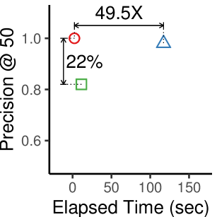
(a) Precision@50 vs. time taken

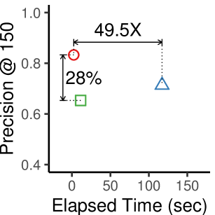
(b) Precision@150 vs. time taken

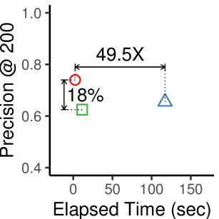
(c) Precision@200 vs. time taken

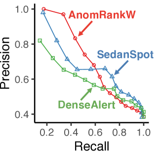
(d) Precision vs. Recall

Figure 3. AnomRank is fastest and most accurate: (a-c) AnomRank outperforms the baselines in terms of both accuracy and speed on the DARPA dataset. (d) AnomRank achieves better precision and recall on high ranks (top-$50,\dots,250$) than its competitors.

5.2. Practicality

We examine the practicality of AnomRank on the DARPA dataset, a public benchmark for Network Intrusion Detection Systems. In this network intrusion setting, our focus is on detecting high-volume (i.e. high edge-weight) intrusions such as denial of service (DOS) attacks, which are typically the focus of graph mining-based detection approaches. Hence, we use only the AnomRankW metric.

Precision and Recall: Using each method, we first compute anomaly scores for each of the $1139$ graph snapshots, then select the top-k most anomalous snapshots ($k=50,100,\cdots,800$). Then we compute precision and recall for each method’s output. In Figure 3(d), AnomRank shows higher precision and recall than DenseAlert and SedanSpot on high ranks (top-$50,\dots,250$). Considering that anomaly detection tasks in real-world settings are generally focused on the most anomalous instances, high accuracy on high ranks is more meaningful than high accuracy on low ranks. Moreover, considering that the number of ground truth anomalies is $288$, its precision and recall up to top-$250$ better reflects its practicality.

Accuracy vs. Running Time: In Figures 1(a) and 3(a-c), AnomRank is most accurate and fastest. Compared to SedanSpot, AnomRank achieves up to $18\%$ higher precision on top-k ranks with $49.5\times$ faster speed. Compared to DenseAlert, AnomRank achieves up to $35\%$ higher precision with $4.8\times$ faster speed. DenseAlert and SedanSpot require several subprocesses (hashing, random-walking, reordering, sampling, etc), resulting in large computation time.

Scalability: Figure 1(b) shows the scalability of AnomRank with the number of edges. We plot the wall-clock time needed to run on the (chronologically) first $2,2^{2},\dots,2^{22}$ edges of the DARPA dataset. This confirms the linear scalability of AnomRank with respect to the number of edges in the input dynamic graph. Note that AnomRank processes $1M$ edges within $1$ second, allowing real-time anomaly detection.

Effectiveness: Figure 1(c) shows changes of AnomRank scores in the DARPA dataset, with time window of $\Delta T=1$ hour. Consistently with the large upper bounds shown in Theorems 1 and 2, ground truth attacks (red crosses) have large AnomRank scores in Figure 1(c). Given mean and std of anomaly scores of all snapshots, setting an anomalousness threshold of (mean + $\frac{1}{2}$std), $77\%$ of spikes above the threshold are true positives. This shows the effectiveness of AnomRank as a barometer of anomalousness.

5.3. Effectiveness of Two-Pronged Approach

In this experiment, we show the effectiveness of our two-pronged approach using real-world and synthetic graphs.

5.3.1. Real-World Graph

We measure anomaly scores based on four metrics: AnomRankS, AnomRankW, SedanSpot, and DenseAlert, on the ENRON dataset. In Figure 4, AnomRankW and SedanSpot show similar trends, while AnomRankS detects different events as anomalies on the same dataset. DenseAlert shows similar trends with the sum of AnomRankS and AnomRankW, while missing several anomalous events. This is also reflected in the low accuracy of DenseAlert on the DARPA dataset in Figure 3. The anomalies detected by AnomRankS and AnomRankW coincide with major events in the ENRON timeline as follows:

1. June 12, 2000: Skilling makes joke at Las Vegas conference, comparing California to the Titanic.

2. August 23, 2000: FERC orders an investigation into Timothy Belden’s strategies designed to drive electricity prices up in California.

3. Oct. 3, 2000: Enron attorney Richard Sanders travels to Portland to discuss Timothy Belden’s strategies.

4. Dec. 13, 2000: Enron announces that Jeffrey Skilling will take over as chief executive.

5. Mar. 2001: Enron transfers large portions of EES business into wholesale to hide EES losses.

6. July 13, 2001: Skilling announces desire to resign to Lay. Lay asks Skilling to take the weekend and think it over.

7. Oct. 17, 2001: Wall Street Journal reveals the precarious nature of Enron’s business.

8. Nov. 19, 2001: Enron discloses it is trying to restructure a 690 million obligation.

9. Jan. 23-25, 2002: Lay resigns as chairman and CEO of Enron. Cliff Baxter, former Enron vice chairman, commits suicide.

10. Feb. 2, 2002: The Powers Report, a summary of an internal investigation into Enron’s collapse spreads out.

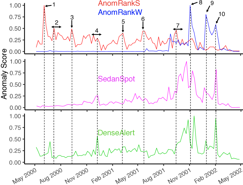
Figure 4. Two-pronged approach pays off: AnomRankW and SedanSpot show similar trends on the Enron dataset, while AnomRankS detects different events as anomalies on the same dataset. DenseAlert shows similar trends with the sum of AnomRankS and AnomRankW while missing several anomalous events.

The high anomaly scores of AnomRankS coincide with the timeline events when Enron conspired to drive the California electricity price up (Events 1,2,3) and office politics played out in Enron (Events 4,5,6). Meanwhile, AnomRankW shows high anomaly scores when the biggest scandals of the company continued to unfold (Events 7, 8,9,10). Note that AnomRankS and AnomRankW are designed to detect different properties of anomalies on dynamic graphs. AnomRankS is effective at detecting AnomalyS like unusual email communications for conspiration, while AnomRankW is effective at detecting AnomalyW like massive email communications about big scandals that swept the whole company. The non-overlapping trends of AnomRankS and AnomRankW show that the two metrics complement each other successfully in real-world data. Summarizing the two observations we make:

• Observation 1. AnomRankS and AnomRankW spot different types of anomalous events.

• Observation 2. DenseAlert and SedanSpot detect a subset of the anomalies detected by AnomRank.

5.3.2. Synthetic Graph

In our synthetic graph generated by RTM method, we inject two types of anomalies to examine the effectiveness of our two metrics. Details of the injections are as follows:

• InjectionS: We choose $50$ timestamps uniformly at random: at each chosen timestamp, we select $8$ nodes uniformly at random, and introduce all edges between these nodes in both directions.

• InjectionW: We choose $50$ timestamps uniformly at random: at each chosen timestamp, we select two nodes uniformly at random, and add $70$ edges from the first to the second.

A clique is an example of AnomalyS with unusual structure pattern, while high edge weights are an example of AnomalyW. Hence, InjectionS and InjectionW are composed of AnomalyS and AnomalyW, respectively.

Then we evaluate the precision of the top-50 highest anomaly scores output by the AnomRankS metric and the AnomRankW metric. We also evaluate each metric on the DARPA dataset based on their top-250 anomaly scores. In Table 3, AnomRankS shows higher precision on InjectionS than AnomRankW, while AnomRankW has higher precision on InjectionW and DARPA. In Section 4.2.3, we showed theoretically that AnomalyS induces larger changes in AnomRankS than AnomRankW, explaining the higher precision of AnomRankS than AnomRankW on InjectionS. We also showed that adding additional edge weights has no effect on AnomRankS, explaining that AnomRankS does not work on InjectionW. For the DARPA dataset, AnomRankW shows higher accuracy than AnomRankS. DARPA contains 2.7M attacks, and $90\%$ of the attacks (2.4M attacks) are DOS attacks generated from only 2-3 source IP adderesses toward 2-3 target IP addresses. These attacks are of AnomalyW type with high edge weights. Thus AnomRankW shows higher precision on DARPA than AnomRankS.

Table 3. AnomRankS and AnomRankW complement each other:
we measure precision of the two metrics on the synthetic graph with two injection scenarios (InjectionS, InjectionW) and the real-world graph DARPA. We measure precision on top-50 and top-250 ranks on the synthetic graph and DARPA, respectively.

	InjectionS	InjectionW	DARPA
AnomRankS only	.96	.00	.42
AnomRankW only	.82	.79	.69

Table 4. 1st and 2nd order derivatives complement each other:
AnomRankW-1st and AnomRankW-2nd are 1st and 2nd derivatives of ScoreW. Combining AnomRankW-1st and AnomRankW-2nd results in the highest precision.

	InjectionS	InjectionW	DARPA
AnomRankW-1st	.06	.11	.65
AnomRankW-2nd	.80	.78	.61
AnomRankW	.82	.79	.69

5.4. Effectiveness of Two-Derivatives Approach

In this experiment, we show the effectiveness of 1st and 2nd order derivatives of ScoreS and ScoreW in detecting anomalies in dynamic graphs. For brevity, we show the result on ScoreW; result on ScoreS is similar. Recall that AnomRankW score is defined as the L1 length of $\mathbf{a}_{w}=[\mathbf{p}_{w}^{\prime}~{}\mathbf{p}_{w}^{\prime\prime}]$ where $\mathbf{p}_{w}^{\prime}$ and $\mathbf{p}_{w}^{\prime\prime}$ are the 1st and 2nd order derivatives of ScoreW, respectively. We define two metrics, AnomRankW-1st and AnomRankW-2nd, which denote the L1 lengths of $\mathbf{p}_{w}^{\prime}$ and $\mathbf{p}_{w}^{\prime\prime}$, respectively. By estimating precision using AnomRankW-1st and AnomRankW-2nd individually, we examine the effectiveness of each derivative using the same injection scenarios and evaluation approach as Section 5.3.2.

In Table 4, AnomRankW-1st shows higher precision on the DARPA dataset, while AnomRankW-2nd has higher precision on injection scenarios. AnomRankW-1st detects suspiciously large anomalies based on L1 length of 1st order derivatives, while AnomRa nkW-2nd detects abruptness of anomalies based on L1 length of 2nd order derivatives. Note that combining 1st and 2nd order derivatives leads to better precision. This shows that 1st and 2nd order derivatives complement each other.

5.5. Attribution

In this experiment, we show that AnomRank successfully localizes the culprits of anomalous events as explained in the last paragraph of Section 4.4. In Figure 5, given a graph snapshot detected as an anomaly in the DARPA dataset, nodes (IP addresses) are sorted in order of their AnomRank scores. Outliers with significantly large scores correspond to IP addresses which are likely to be engaged in network intrusion attacks. At the $15$th snapshot ($T=15$) when Back DOS attacks occur, the attacker IP ($135.008.060.182$) and victim IP ($172.016.114.050$) have the largest AnomRank scores. In the $133$th snapshot ($T=133$) where Nmap probing attacks take place, the victim IP ($172.016.112.050$) has the largest score.

6. Conclusion

In this paper, we proposed a two-pronged approach for detecting anomalous events in a dynamic graph.

Our main contributions are:

• Online, Two-Pronged Approach We introduced AnomRank, a novel and simple detection method in dynamic graphs.

• Theoretical Guarantees We present theoretical analysis (Theorems 1 and 2) on the effectiveness of AnomRank.

• Practicality In Section 5, we show that AnomRank outperforms state-of-the-art baselines, with up to $\mathit{49.5\times}$ faster speed or $\mathit{35\%}$ higher accuracy. AnomRank is fast, taking about 2 seconds on a graph with 4.5 million edges.

Our code and data are publicly available.

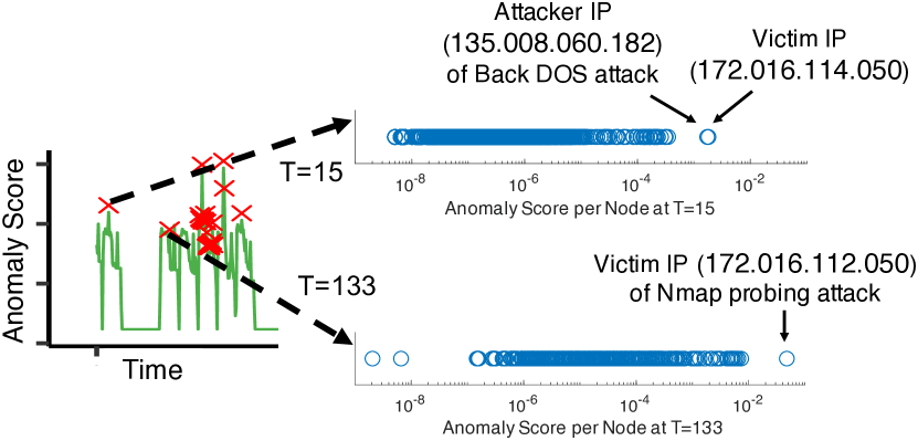
Figure 5. Attribution: AnomRank localizes the culprits of anomalous events in the DARPA dataset: in a Back DOS attack, the attacker and victim IP have the top-2 largest scores; in an Nmap probing attack, the victim IP has the largest AnomRank score.

Appendix A Supplement

A.1. Experimental Setting

All experiments are carried out on a 3 GHz Intel Core i5 iMac, 16 GB RAM, running OS X 10.13.6. We implemented AnomRank and SedanSpot in C++, and we used an open-sourced implementation of DenseAlert, provided by the authors of (Shin et al., 2017). To show the best trade-off between speed and accuracy, we set the sample size to 50 for SedanSpot and follow other parameter settings as suggested in the original paper (Eswaran and Faloutsos, 2018). For AnomRank, we set the damping factor $c$ to $0.5$, and stop iterations for computing node score vectors when $L1$ changes of node score vectors are less than $10^{-3}$.

A.2. Dataset

DARPA (Lippmann et al., 1999) has 4.5M IP-IP communications between 9.4K source IP and 2.3K destination IP over 87.7K minutes. Each communication is a directed edge (srcIP, dstIP, timestamp, attack) where the attack label indicates whether the communication is an attack or not. We aggregate edges occurring in every hour, resulting in a stream of 1463 graphs. We annotate a graph snapshot as anomalous if it contains at least 50 attack edges. Then there are 288 ground truth anomalies ($23.8\%$ of total). We use the first 256 graphs for initializing means and variances needed during normalization (as described in Section 4.4).

ENRON (Shetty and Adibi, 2004) contains 50K emails from 151 employees over 3 years in the ENRON Corporation. Each email is a directed edge (sender, receiver, timestamp). We aggregate edges occurring in every day duration, resulting in a stream of 1139 graphs. We use the first 256 graphs for initializing means and variances.

RTM method (Akoglu et al., 2008) generates time-evolving graphs with repeated Kronecker products. We use the publicly available code. The generated graph is a directed graph with 1K nodes and 8.1K edges over 2.7K timestamps. We use the first 300 timestamps for initializing means and variances.

A.3. Proofs

We prove upper bounds on the 1st and 2nd derivatives of ScoreS and ScoreW, showing their effectiveness in detecting AnomalyS and AnomalyW.

Proof of Lemma 5 (Upper bound of $\lVert\mathbf{p}_{s}^{\prime}\rVert_{1}$).

For brevity, $\mathbf{p}_{s}^{n}\leftarrow\mathbf{p}_{s}(t+\Delta t),\mathbf{p}_{s}^{o}\leftarrow\mathbf{p}_{s}(t)$. By Lemma 1, $\lVert\mathbf{p}_{s}^{n}-\mathbf{p}_{s}^{o}\rVert_{1}$ is presented as follows:

$$\lVert\mathbf{p}_{s}^{n}-\mathbf{p}_{s}^{o}\rVert_{1} =\lVert\sum_{k=0}^{\infty}c^{k}(\mathbf{\tilde{A}}_{s}^{\top}+\Delta\mathbf{A}_{s})^{k}c(\Delta\mathbf{A}_{s}\mathbf{p}_{s}^{o})\rVert_{1}$$

$$\leq c\sum_{k=0}^{\infty}\lVert c^{k}(\mathbf{\tilde{A}}_{s}^{\top}+\Delta\mathbf{A}_{s})^{k}\rVert_{1}\lVert\Delta\mathbf{A}_{s}\mathbf{p}_{s}^{o}\rVert_{1}$$

$$\leq\frac{c}{1-c}\lVert\Delta\mathbf{A}_{s}\mathbf{p}_{s}^{o}\rVert_{1}\leq\frac{c}{1-c}\lVert\Delta\mathbf{A}_{s}\rVert_{1}$$

$$\lVert\mathbf{p}_{s}^{\prime}\rVert_{1} =\lVert\frac{\mathbf{p}_{s}^{n}-\mathbf{p}_{s}^{o}}{\Delta t}\rVert_{1}\leq\frac{c}{1-c}\lVert\frac{\Delta\mathbf{A}_{s}}{\Delta t}\rVert_{1}$$

Note that $\lVert(\mathbf{\tilde{A}}_{s}^{\top}+\Delta\mathbf{A}_{s})^{k}\rVert_{1}=\lVert\mathbf{p}_{s}^{o}\rVert_{1}=1$ since $(\mathbf{\tilde{A}}_{s}^{\top}+\Delta\mathbf{A}_{s})$ is a column-normalized stochastic matrix, and $\mathbf{p}_{s}^{o}$ is a PageRank vector. $\hfill\blacksquare$

Proof of Lemma 6 (Upper bound of $\lVert\mathbf{p}_{s}^{\prime\prime}\rVert_{1}$).

For brevity, $\mathbf{p}_{0}\leftarrow\mathbf{p}_{s}(t-\Delta t),\mathbf{p}_{1}\leftarrow\mathbf{p}_{s}(t),\mathbf{p}_{2}\leftarrow\mathbf{p}_{s}(t+\Delta t),\Delta\mathbf{p}^{o}\leftarrow\mathbf{p}_{1}-\mathbf{p}_{0},\Delta\mathbf{p}^{n}\leftarrow\mathbf{p}_{2}-\mathbf{p}_{1},\mathbf{A}\leftarrow\mathbf{\tilde{A}}_{s}^{\top},\Delta\mathbf{A}_{1}\leftarrow\Delta\mathbf{A}_{s_{o}}$ and $\Delta\mathbf{A}_{2}\leftarrow\Delta\mathbf{A}_{s_{n}}$. In addition, we omit $c$ by substituting $\mathbf{A}\leftarrow c\mathbf{A}$ and $\Delta\mathbf{A}\leftarrow c\Delta\mathbf{A}$ during this proof. By Lemma 1, $\Delta\mathbf{p}^{n}$ is:

$$\Delta\mathbf{p}^{n} =\sum_{k=0}^{\infty}(\mathbf{A}+\Delta\mathbf{A}_{1}+\Delta\mathbf{A}_{2})^{k}(\Delta\mathbf{A}_{2}\mathbf{p}_{1})$$

$\Delta\mathbf{p}^{n}$ can be viewed as an updated ScoreS with the original adjacency matrix $Y_{1}=(\mathbf{A}+\Delta\mathbf{A}_{1})$, the update $\Delta\mathbf{A}_{2}$, and the starting vector $(\Delta\mathbf{A}_{2}\mathbf{p}_{1})$ from an original vector $\mathbf{p}_{temp}=\sum_{k=0}^{\infty}Y_{1}^{k}(\Delta\mathbf{A}_{2}\mathbf{p}_{1})$. Then, by Lemma 1, $\Delta\mathbf{p}^{n}$ is presented as follows:

$$\Delta\mathbf{p}^{n} =\mathbf{p}_{temp}+\sum_{k=0}^{\infty}(Y_{1}+\Delta\mathbf{A}_{2})^{k}\Delta\mathbf{A}_{2}\mathbf{p}_{temp}$$

$$=\sum_{k=0}^{\infty}Y_{1}^{k}(\Delta\mathbf{A}_{2}\mathbf{p}_{1})+\sum_{k=0}^{\infty}(Y_{1}+\Delta\mathbf{A}_{2})^{k}\Delta\mathbf{A}_{2}\sum_{i=0}^{\infty}Y_{1}^{i}(\Delta\mathbf{A}_{2}\mathbf{p}_{1})$$

Then $\Delta\mathbf{p}^{n}-\Delta\mathbf{p}^{o}$ becomes as follows:

$$\Delta\mathbf{p}^{o} =\sum_{k=0}^{\infty}(\mathbf{A}+\Delta\mathbf{A}_{1})^{k}(\Delta\mathbf{A}_{1}\mathbf{p}_{0})=\sum_{k=0}^{\infty}Y_{1}^{k}(\Delta\mathbf{A}_{1}\mathbf{p}_{0})$$

$$\Delta\mathbf{p}^{n}-\Delta\mathbf{p}^{o}= \sum_{k=0}^{\infty}Y_{1}^{k}(\Delta\mathbf{A}_{2}-\Delta\mathbf{A}_{1})\mathbf{p}_{1}+\sum_{k=0}^{\infty}Y_{1}^{k}\Delta\mathbf{A}_{1}(\mathbf{p}_{1}-\mathbf{p}_{0})$$

$$+\sum_{k=0}^{\infty}(Y_{1}+\Delta\mathbf{A}_{2})^{k}\Delta\mathbf{A}_{2}\sum_{i=0}^{\infty}Y_{1}^{i}(\Delta\mathbf{A}_{2}\mathbf{p}_{1})$$

Since $\mathbf{p}_{1}-\mathbf{p}_{0}=\Delta\mathbf{p}^{o}=\sum_{k=0}^{\infty}Y_{1}^{k}(\Delta\mathbf{A}_{1}\mathbf{p}_{0})$, the second term $\sum_{k=0}^{\infty}Y_{1}^{k}\Delta\mathbf{A}_{1}(\mathbf{p}_{1}-\mathbf{p}_{0})$ in the equation above is:

$$\sum_{k=0}^{\infty}Y_{1}^{k}\Delta\mathbf{A}_{1}(\mathbf{p}_{1}-\mathbf{p}_{0})=\sum_{k=0}^{\infty}Y_{1}^{k}\Delta\mathbf{A}_{1}\sum_{i=0}^{\infty}Y_{1}^{i}(\Delta\mathbf{A}_{1}\mathbf{p}_{0})$$

Note that$\lVert\mathbf{p}_{0}\rVert_{1}=\lVert\mathbf{p}_{1}\rVert_{1}=1$ since $\mathbf{p}_{0}$ and $\mathbf{p}_{1}$ are PageRank vectors. Recovering $c$ from $\mathbf{A}$ and $\Delta\mathbf{A}$, $\lVert\sum_{k=0}^{\infty}Y_{1}^{k}\rVert_{1}$ and $\lVert\sum_{k=0}^{\infty}(Y_{1}+\Delta\mathbf{A}_{2})^{k}\rVert_{1}$ becomes as follows:

$$\lVert\sum_{k=0}^{\infty}Y_{1}^{k}\rVert_{1} =\lVert\sum_{k=0}^{\infty}c^{k}(\mathbf{A}+\Delta\mathbf{A}_{1})^{k}\rVert_{1}=\frac{1}{1-c}$$

$$\lVert\sum_{k=0}^{\infty}(Y_{1}+\Delta\mathbf{A}_{2})^{k}\rVert_{1} =\lVert\sum_{k=0}^{\infty}c^{k}(\mathbf{A}+\Delta\mathbf{A}_{1}+\Delta\mathbf{A}_{2})^{k}\rVert_{1}=\frac{1}{1-c}$$

Note that $\mathbf{A}+\Delta\mathbf{A}_{1}$ and $\mathbf{A}+\Delta\mathbf{A}_{1}+\Delta\mathbf{A}_{2}$ are column-normalized stochastic matrices. Then $\lVert\Delta\mathbf{p}^{n}-\Delta\mathbf{p}^{o}\rVert_{1}$ is bounded as follow:

$$\lVert\Delta\mathbf{p}^{n}-\Delta\mathbf{p}^{o}\rVert_{1}\leq\frac{c}{1-c}\lVert\Delta\mathbf{A}_{2}-\Delta\mathbf{A}_{1}\rVert_{1}+(\frac{c}{1-c})^{2}(\lVert\Delta\mathbf{A}_{1}\rVert_{1}^{2}+\lVert\Delta\mathbf{A}_{2}\rVert_{1}^{2})$$

Then, recovering $c$ from all terms, $\lVert\mathbf{p}_{s}^{\prime\prime}\rVert_{1}$ is bounded as follows:

$$\lVert\mathbf{p}_{s}^{\prime\prime}\rVert_{1}=\frac{\lVert\Delta\mathbf{p}^{n}-\Delta\mathbf{p}^{o}\rVert_{1}}{\Delta t^{2}}$$

$$\leq\frac{\frac{c}{1-c}\lVert\Delta\mathbf{A}_{2}-\Delta\mathbf{A}_{1}\rVert_{1}+(\frac{c}{1-c})^{2}(\lVert\Delta\mathbf{A}_{1}\rVert_{1}^{2}+\lVert\Delta\mathbf{A}_{2}\rVert_{1}^{2})}{\Delta t^{2}}$$

$\hfill\blacksquare$

Proof of Theorem 1.

(Upper bounds of $\lVert\mathbf{p}_{s}^{\prime}\rVert_{1}$ and $\lVert\mathbf{p}_{s}^{\prime\prime}\rVert_{1}$ with AnomalyS) Use Lemma 3 and 5. $\hfill\blacksquare$

Proof of Lemma 7 (Upper bounds of $\lVert\mathbf{p}_{w}^{\prime}\rVert_{1}$).

For brevity, denote $\mathbf{p}_{w}^{o}\leftarrow\mathbf{p}_{w}(t)$ and $\mathbf{p}_{w}^{n}\leftarrow\mathbf{p}_{w}(t+\Delta t)$. By Lemma 2, $\lVert\mathbf{p}_{w}^{n}-\mathbf{p}_{w}^{o}\rVert_{1}$ is presented as follows:

$$\mathbf{p}_{w}^{n}-\mathbf{p}_{w}^{o}=~{} \sum_{k=0}^{\infty}c^{k}(\mathbf{\tilde{A}}_{w}^{\top}+\Delta\mathbf{A}_{w})^{k}c\Delta\mathbf{A}_{w}\mathbf{p}_{w}^{o}$$

$$+(1-c)\sum_{k=0}^{\infty}c^{k}(\mathbf{\tilde{A}}_{w}^{\top}+\Delta\mathbf{A}_{w})^{k}\Delta\mathbf{b}_{w}$$

$$\lVert\mathbf{p}_{w}^{n}-\mathbf{p}_{w}^{o}\rVert_{1}\leq~{} \frac{c}{1-c}\lVert\Delta\mathbf{A}_{w}\rVert_{1}+\lVert\Delta\mathbf{b}_{w}\rVert_{1}$$

$$\lVert\mathbf{p}_{w}^{\prime}\rVert_{1}=~{} \frac{\lVert\mathbf{p}_{w}^{n}-\mathbf{p}_{w}^{o}\rVert_{1}}{\Delta t}\leq\frac{1}{\Delta t}(\frac{c}{1-c}\lVert\Delta\mathbf{A}_{w}\rVert_{1}+\lVert\Delta\mathbf{b}_{w}\rVert_{1})$$

$\lVert(\mathbf{\tilde{A}}_{w}^{\top}+\Delta\mathbf{A}_{w})^{k}\rVert_{1}=\lVert\mathbf{p}_{w}^{o}\rVert_{1}=1$ since $\mathbf{\tilde{A}}_{w}^{\top}+\Delta\mathbf{A}_{w}$ is a column-normalized stochastic matrix and $\mathbf{p}_{w}^{o}$ is a PageRank vector. $\hfill\blacksquare$

Proof of Lemma 8 (Upper bound of $\lVert\mathbf{p}_{w}^{\prime\prime}\rVert_{1}$).

For brevity, denote $\mathbf{p}_{0}\leftarrow\mathbf{p}_{w}(t-\Delta t),\mathbf{p}_{1}\leftarrow\mathbf{p}_{w}(t),\mathbf{p}_{2}\leftarrow\mathbf{p}_{w}(t+\Delta t),\Delta\mathbf{p}^{o}\leftarrow\mathbf{p}_{1}-\mathbf{p}_{0},\Delta\mathbf{p}^{n}\leftarrow\mathbf{p}_{2}-\mathbf{p}_{1},\mathbf{A}\leftarrow\mathbf{\tilde{A}}_{w}^{\top},\Delta\mathbf{A}_{1}\leftarrow\Delta\mathbf{A}_{w_{o}},\Delta\mathbf{A}_{2}\leftarrow\Delta\mathbf{A}_{w_{n}},\Delta\mathbf{b}_{1}\leftarrow\Delta\mathbf{b}_{w_{o}}$ and $\Delta\mathbf{b}_{2}\leftarrow\Delta\mathbf{b}_{w_{n}}$. In addition, we omit the $c$ term by substituting $\mathbf{A}\leftarrow c\mathbf{A},\Delta\mathbf{A}\leftarrow c\Delta\mathbf{A}$ and $\Delta\mathbf{b}\leftarrow(1-c)\Delta\mathbf{b}$ during this proof. By Lemma 2, $\Delta\mathbf{p}^{o}$ and $\Delta\mathbf{p}^{n}$ are presented as follows:

$$\Delta\mathbf{p}^{o} =\sum_{k=0}^{\infty}(\mathbf{A}+\Delta\mathbf{A}_{1})^{k}\Delta\mathbf{A}_{1}\mathbf{p}_{0}+\sum_{k=0}^{\infty}(\mathbf{A}+\Delta\mathbf{A}_{1})^{k}\Delta\mathbf{b}_{1}$$

$$\Delta\mathbf{p}^{n} =\sum_{k=0}^{\infty}(\mathbf{A}+\Delta\mathbf{A}_{1}+\Delta\mathbf{A}_{2})^{k}\Delta\mathbf{A}_{2}\mathbf{p}_{1}+\sum_{k=0}^{\infty}(\mathbf{A}+\Delta\mathbf{A}_{1}+\Delta\mathbf{A}_{2})^{k}\Delta\mathbf{b}_{2}$$

Substracting the first term of $\Delta\mathbf{p}^{o}$ from the first term of $\Delta\mathbf{p}^{n}$ is equal to $\mathbf{p}_{s}^{\prime\prime}$ as shown in Lemma 6. Then $\Delta\mathbf{p}^{n}-\Delta\mathbf{p}^{o}$ is:

$$\Delta\mathbf{p}^{n}-\Delta\mathbf{p}^{o}=\mathbf{p}_{s}^{\prime\prime}+\sum_{k=0}^{\infty}(\mathbf{A}+\Delta\mathbf{A}_{1}+\Delta\mathbf{A}_{2})^{k}\Delta\mathbf{b}_{2}-\sum_{k=0}^{\infty}(\mathbf{A}+\Delta\mathbf{A}_{1})^{k}\Delta\mathbf{b}_{1}$$

By substituting $\mathbf{A}+\Delta\mathbf{A}_{1}$ with $Y_{2}$, the last two terms in the above equation are presented as follows:

$$\sum_{k=0}^{\infty}(Y_{2}+\Delta\mathbf{A}_{2})^{k}\Delta\mathbf{b}_{2}-\sum_{k=0}^{\infty}Y_{2}^{k}\Delta\mathbf{b}_{1}$$

$$=\sum_{k=0}^{\infty}Y_{2}^{k}\Delta\mathbf{b}_{2}+\sum_{k=0}^{\infty}(Y_{2}+\Delta\mathbf{A}_{2})^{i}\Delta\mathbf{A}_{2}\sum_{i=0}^{\infty}Y_{2}^{k}\Delta\mathbf{b}_{2}-\sum_{k=0}^{\infty}Y_{2}^{k}\Delta\mathbf{b}_{1}$$

$$=\sum_{k=0}^{\infty}Y_{2}^{k}(\Delta\mathbf{b}_{2}-\Delta\mathbf{b}_{1})+\sum_{k=0}^{\infty}(Y_{2}+\Delta\mathbf{A}_{2})^{i}\Delta\mathbf{A}_{2}\sum_{i=0}^{\infty}Y_{2}^{k}\Delta\mathbf{b}_{2}$$

In the first equation, we treat $\sum_{k=0}^{\infty}(Y_{2}+\Delta\mathbf{A}_{2})^{k}\Delta\mathbf{b}_{2}$ as an updated PageRank with the update $\Delta\mathbf{A}_{2}$ from an original PageRank $\sum_{k=0}^{\infty}Y_{2}^{k}\Delta\mathbf{b}_{2}$, then apply Lemma 1. Note that both $\lVert\sum_{k=0}^{\infty}Y_{2}^{k}\rVert_{1}$ and $\lVert\sum_{k=0}^{\infty}(Y_{2}+\Delta\mathbf{A}_{2})^{k}\rVert_{1}$ have value $\frac{1}{1-c}$ since the original expressions with $c$ terms are as follows:

$$\sum_{k=0}^{\infty}Y_{2}^{k} =\sum_{k=0}^{\infty}c^{k}(\mathbf{\tilde{A}}_{w}^{\top}+\Delta\mathbf{A}_{w_{o}})^{k}$$

$$\sum_{k=0}^{\infty}(Y_{2}+\Delta\mathbf{A}_{2})^{k} =\sum_{k=0}^{\infty}c^{k}(\mathbf{\tilde{A}}_{w}^{\top}+\Delta\mathbf{A}_{w_{o}}+\Delta\mathbf{A}_{w_{n}})^{k}$$

$(\mathbf{\tilde{A}}_{w}^{\top}+\Delta\mathbf{A}_{w_{o}})$ and $(\mathbf{\tilde{A}}_{w}^{\top}+\Delta\mathbf{A}_{w_{o}}+\Delta\mathbf{A}_{w_{n}})$ are column-normalized stochastic matrices. Then, recovering $c$ from all terms, $\lVert\mathbf{p}_{w}^{\prime\prime}\rVert_{1}$ is bounded as follow:

$$\frac{\lVert\Delta\mathbf{p}^{n}-\Delta\mathbf{p}^{o}\rVert_{1}}{\Delta t^{2}} \leq\lVert\mathbf{p}_{s}^{\prime\prime}\rVert_{max}$$

$$+\frac{1}{\Delta t^{2}}(\lVert\Delta\mathbf{b}_{2}-\Delta\mathbf{b}_{1}\rVert_{1}+\frac{c}{1-c}\lVert\Delta\mathbf{A}_{2}\rVert_{1}\lVert\Delta\mathbf{b}_{2}\rVert_{1})$$

$\hfill\blacksquare$

Proof of Theorem 2.

(Upper bounds of $\lVert\mathbf{p}_{w}^{\prime}\rVert_{1}$ and $\lVert\mathbf{p}_{w}^{\prime\prime}\rVert_{1}$ with AnomalyW) Use Lemma 4, 6 and 8. $\hfill\blacksquare$

References

- (1)
- Aggarwal et al. (2011) Charu C Aggarwal, Yuchen Zhao, and Philip S Yu. 2011. Outlier detection in graph streams. In ICDE.
- Akoglu et al. (2008) Leman Akoglu, Mary McGlohon, and Christos Faloutsos. 2008. RTM: Laws and a recursive generator for weighted time-evolving graphs. In ICDM.
- Akoglu et al. (2010) Leman Akoglu, Mary McGlohon, and Christos Faloutsos. 2010. Oddball: Spotting anomalies in weighted graphs. In PAKDD.
- Akoglu et al. (2015) Leman Akoglu, Hanghang Tong, and Danai Koutra. 2015. Graph based anomaly detection and description: a survey. DMKD 29, 3 (2015), 626–688.
- Beutel et al. (2013) Alex Beutel, Wanhong Xu, Venkatesan Guruswami, Christopher Palow, and Christos Faloutsos. 2013. Copycatch: stopping group attacks by spotting lockstep behavior in social networks. In WWW.
- Chakrabarti (2004) Deepayan Chakrabarti. 2004. Autopart: Parameter-free graph partitioning and outlier detection. In PKDD.
- Chung (1994) F.R.K. Chung. 1994. Spectral Graph Theory. Number no. 92 in CBMS Regional Conference Series. Conference Board of the Mathematical Sciences.
- Eswaran and Faloutsos (2018) Dhivya Eswaran and Christos Faloutsos. 2018. SEDANSPOT: Detecting Anomalies in Edge Streams. In ICDM.
- Eswaran et al. (2018) Dhivya Eswaran, Christos Faloutsos, Sudipto Guha, and Nina Mishra. 2018. SpotLight: Detecting Anomalies in Streaming Graphs. In KDD.
- Henderson et al. (2010) Keith Henderson, Tina Eliassi-Rad, Christos Faloutsos, Leman Akoglu, Lei Li, Koji Maruhashi, B Aditya Prakash, and Hanghang Tong. 2010. Metric forensics: a multi-level approach for mining volatile graphs. In KDD.
- Hooi et al. (2017) Bryan Hooi, Kijung Shin, Hyun Ah Song, Alex Beutel, Neil Shah, and Christos Faloutsos. 2017. Graph-based fraud detection in the face of camouflage. TKDD 11, 4 (2017), 44.
- Jiang et al. (2016) Meng Jiang, Peng Cui, Alex Beutel, Christos Faloutsos, and Shiqiang Yang. 2016. Catching synchronized behaviors in large networks: A graph mining approach. TKDD 10, 4 (2016), 35.
- Kleinberg (1999) Jon M Kleinberg. 1999. Authoritative sources in a hyperlinked environment. JACM 46, 5 (1999), 604–632.
- Koutra et al. (2016) Danai Koutra, Neil Shah, Joshua T Vogelstein, Brian Gallagher, and Christos Faloutsos. 2016. DeltaCon: principled massive-graph similarity function with attribution. TKDD 10, 3 (2016), 28.
- Lempel and Moran (2001) Ronny Lempel and Shlomo Moran. 2001. SALSA: the stochastic approach for link-structure analysis. ACM Trans. Inf. Syst. 19, 2 (2001), 131–160.
- Lippmann et al. (1999) Richard Lippmann, Robert K Cunningham, David J Fried, Isaac Graf, Kris R Kendall, Seth E Webster, and Marc A Zissman. 1999. Results of the DARPA 1998 Offline Intrusion Detection Evaluation.. In Recent advances in intrusion detection, Vol. 99. 829–835.
- Page et al. (1999) Lawrence Page, Sergey Brin, Rajeev Motwani, and Terry Winograd. 1999. The PageRank citation ranking: Bringing order to the web. Technical Report. Stanford InfoLab.
- Ranshous et al. (2016) Stephen Ranshous, Steve Harenberg, Kshitij Sharma, and Nagiza F Samatova. 2016. A scalable approach for outlier detection in edge streams using sketch-based approximations. In SDM.
- Shetty and Adibi (2004) Jitesh Shetty and Jafar Adibi. 2004. The Enron email dataset database schema and brief statistical report. Information sciences institute technical report, University of Southern California 4, 1 (2004), 120–128.
- Shin et al. (2018a) Kijung Shin, Tina Eliassi-Rad, and Christos Faloutsos. 2018a. Patterns and anomalies in k-cores of real-world graphs with applications. KAIS 54, 3 (2018), 677–710.
- Shin et al. (2018b) Kijung Shin, Bryan Hooi, and Christo Faloutsos. 2018b. Fast, Accurate, and Flexible Algorithms for Dense Subtensor Mining. TKDD 12, 3 (2018), 28.
- Shin et al. (2017) Kijung Shin, Bryan Hooi, Jisu Kim, and Christos Faloutsos. 2017. DenseAlert: Incremental dense-subtensor detection in tensor streams. In KDD.
- Sun et al. (2006) Jimeng Sun, Dacheng Tao, and Christos Faloutsos. 2006. Beyond streams and graphs: dynamic tensor analysis. In KDD.
- Tong and Lin (2011) Hanghang Tong and Ching-Yung Lin. 2011. Non-negative residual matrix factorization with application to graph anomaly detection. In SDM.
- Wang et al. (2015) Teng Wang, Chunsheng Fang, Derek Lin, and S Felix Wu. 2015. Localizing temporal anomalies in large evolving graphs. In SDM.
- Wasserman and Faust (1994) Stanley Wasserman and Katherine Faust. 1994. Social network analysis: Methods and applications. Cambridge university press.
- Xu et al. (2007) Xiaowei Xu, Nurcan Yuruk, Zhidan Feng, and Thomas AJ Schweiger. 2007. Scan: a structural clustering algorithm for networks. In KDD.
- Yoon et al. (2018a) Minji Yoon, Woojeong Jin, and U Kang. 2018a. Fast and Accurate Random Walk with Restart on Dynamic Graphs with Guarantees. In WWW.
- Yoon et al. (2018b) Minji Yoon, Jinhong Jung, and U Kang. 2018b. TPA: Fast, Scalable, and Accurate method for Approximate Random Walk with Restart on Billion Scale Graphs. In ICDE.