Omni-GAN: On the Secrets of cGANs and Beyond
Abstract
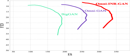
The conditional generative adversarial network (cGAN) is a powerful tool of generating high-quality images, but existing approaches mostly suffer unsatisfying performance or the risk of mode collapse. This paper presents Omni-GAN, a variant of cGAN that reveals the devil in designing a proper discriminator for training the model. The key is to ensure that the discriminator receives strong supervision to perceive the concepts and moderate regularization to avoid collapse. Omni-GAN is easily implemented and freely integrated with off-the-shelf encoding methods (e.g., implicit neural representation, INR). Experiments validate the superior performance of Omni-GAN and Omni-INR-GAN in a wide range of image generation and restoration tasks. In particular, Omni-INR-GAN sets new records on the ImageNet dataset with impressive Inception scores of 262.85 and 343.22 for the image sizes of 128 and 256, respectively, surpassing the previous records by 100+ points. Moreover, leveraging the generator prior, Omni-INR-GAN can extrapolate low-resolution images to arbitrary resolution, even up to higher resolution. Code will be available111https://github.com/PeterouZh/Omni-GAN-PyTorch.
1 Introduction
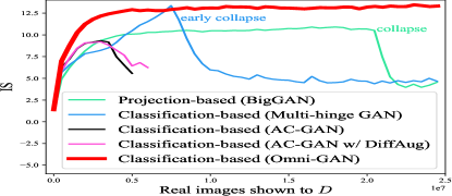
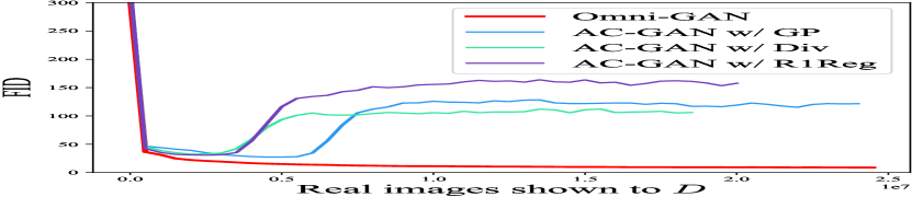
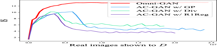
The Generative Adversarial Network (GAN) [19] is a powerful tool for image generation [2, 30, 46] and domain adaptation [8, 26, 39, 70]. The big family of GAN can be roughly divided into two parts, i.e., the unconditional GANs [32, 33] and conditional GANs (cGANs) [45, 6], differing from each other in whether the class labels (e.g., cat, car, flower, etc.) are used for image generation. In practice, cGAN often suffers severe collapse when the number of categories is large. As shown in Fig. 1, all of BigGAN [6], Multi-hinge GAN [34], and AC-GAN [49] achieve high Inception scores, but the curves drop dramatically at some point of training. This makes the cGAN training procedure unstable and thus early termination trick is used by the community [6].
 |
 |
| (a) | (b) |
It has been noticed [31] that the instability of the training procedure is highly related to the discriminator, i.e., the module that outputs a value indicating the reality of the generated image. The existing cGAN discriminators are roughly categorized into two types, namely, the projection-based [47, 6] and classification-based [49, 34] ones, according to whether the discriminator is required to output an explicit class label for each image. We find that, although the former choice (i.e., a projection-based, with a weaker, implicit discriminator) is inferior to the latter in terms of the Inception score, the latter is prone to collapse (e.g., in Fig. 1, Multi-hinge GAN achieves a high Inception score but collapses earlier).
This paper investigates the reason behind this phenomenon. We formulate the classification-based and projection-based discriminator into a multi-label classification framework, which offers us an opportunity to observe the advantages and disadvantages of them. As a result, we find that combining strong supervision (classification loss) and moderate regularization (to prevent it from quickly memorizing the training image set) is the best choice, where the GAN model enjoys high quality in image generation yet has a low risk of mode collapse. In practice, we use weight decay as the choice of regularization, and our algorithm, named Omni-GAN, is easily implemented in any deep learning framework (adding a few lines of code beyond BigGAN). To show that our discovery generalizes to a wide range of cGAN models, we further integrate implicit neural representation (INR) [51, 44, 11], an off-the-shelf encoding method, into Omni-GAN. This not only improves the generation quality of Omni-GAN, but also enables it to generate images of any aspect ratio and any resolution, facilitating its application to downstream tasks.
We validate the advantages of our approach with extensive experiments on image generation and restoration. The image generation task is performed on CIFAR10, CIFAR100 [35], and ImageNet [15], three popular datasets. Omni-GAN surpasses the baselines in terms of the Fréchet Inception distance [22] and Inception score [60]. In particular, in generating and images on ImageNet, Omni-GAN achieves surprising Inception scores of and , respectively, both of which surpassing the previous records by more than points. The image restoration part involves colorization and single image super-resolution, where Omni-INR-GAN is more flexible than BigGAN and significantly outperforms other restoration methods like DIP [71] and LIIF [10], arguably because the prior learned by the generator is stronger.
We highlight the contributions of this paper as follows:
-
•
The core discovery is that combining strong supervision and moderate regularization is the key to cGAN optimization. We achieve this goal easily with the proposed Omni-GAN framework.
-
•
We integrate Omni-GAN into a recently published encoding named INR to validate its generalized ability and extend its range of applications.
-
•
Omni-GAN achieves the state-of-the-art on the task of image generation on ImageNet, surpassing the prior best results by significant margins. It also requires fewer computational costs to gain the ability of high-quality image generation.
We will release the code to the public. We hope that our discovery can inspire the community in studying the principle of generative models and designing powerful algorithms.
2 Preliminaries
2.1 Conditional GANs
Conditional GAN (cGAN) [45] adds conditional information to the generator and discriminator of GANs [28, 27, 1, 2, 43, 58, 22, 29, 4, 61, 69, 12, 18, 41, 55, 9, 63]. There are some ways to incorporate class information into the generator, such as conditional batch normalization (CBN) [14], conditional instance normalization (CIN) [17, 23], class-modulated convolution (CMConv) [82], etc. There are also many ways to add class information to the discriminator. A simple way is to directly concatenate the class information with the input or features from some middle layers [16, 57, 76, 54, 59]. Next, we expound on several slightly complicated methods.
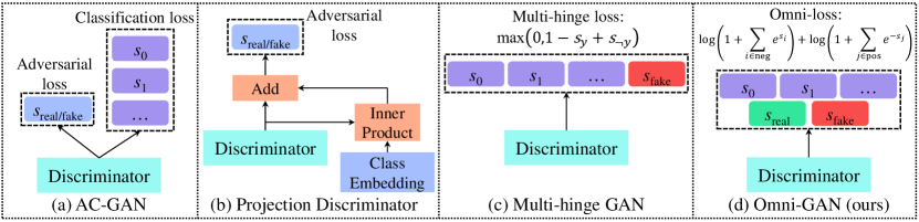
AC-GAN Auxiliary classifier GAN (AC-GAN) [49] uses an auxiliary classifier to enhance the standard GAN model (see Fig. 2a). In particular, the objective function consists of tow parts: the GAN loss, , and the classification loss, :
| (1) | ||||
| (2) |
where g denotes the label of . and represent a real image and a generated image respectively. The discriminator of AC-GAN is trained to maximize , and the generator is trained to maximize . We will show that the discriminator loss of AC-GAN is not optimal (see Sec. 3.3).
Projection Discriminator Projection discriminator [47] incorporates class information into the discriminator of GANs in a projection-based way (see Fig. 2b). The mathematical form of the projection discriminator is given by
| (3) |
where and denote the input image and one-hot label vector respectively. is a class embedding matrix, is a vector function, and is a scalar function. are learned parameters of . The discriminator only outputs a scalar for each pair of and .
2.2 Implicit Neural Representation
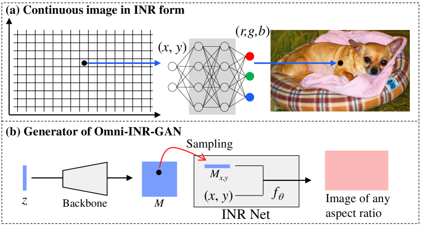
Images are usually represented by a set of pixels with fixed resolution. A popular method named implicit neural representation (INR) is prevalent in the 3D field [51, 44, 11, 3, 20, 7, 53, 25]. Recently, people introduced the INR method to 2D images [10, 65, 64, 5, 66]. The INR of an image directly maps (, ) coordinates to image’s RGB pixel values. Since the coordinates are continuous, once we get the INR of an image, we can get images of arbitrary resolutions by sampling different numbers of coordinates.
2.3 Unified Loss for Feature Learning
There is a unified perspective for classification tasks. We denote the positive score set as , and negative score set as , respectively. Sun et al. [68] proposed a unified loss to maximize as well as to minimize . The loss is defined as
3 Omni-GAN
3.1 Omni-GAN and One-sided Omni-GAN
We commence from defining the omni-loss. Based on this loss, we design two versions of cGANs: Omni-GAN, being a classification-based cGAN, and one-sided Omni-GAN, being a projection-based cGAN. These two cGANs enable us to fairly and intuitively explore the secrets behind classification-based cGANs and projection-based cGANs.
Let and denote an image and its multi-label vector respectively. is a classifier. Suppose that there are positive labels and negative labels. Then is a dimensional score vector. The omni-loss is defined as
|
|
(5) |
where is a set consisting of indexes of negative scores (i.e., ), and consists of indexes of positive scores (i.e., ). represents the element of vector . [67] shows that Eq. (5) is a special case of Eq. (4). We provide a detailed derivation from Eq. (4) to Eq. (5) in Appendix A. Next, we introduce two versions of Omni-GAN by setting different labels for the omni-loss.
The classification-based Omni-GAN.
We first elucidate the loss of the discriminator for Omni-GAN. The discriminator loss consists of two parts, one for (drawn from the training data), and the other for (drawn from the generator). For , its multi-label vector is given by
| (6) |
whose dimension is , with being the number of classes of the training dataset. is if its index in the vector is equal to the ground truth label of , otherwise . We use to denote the corresponding score belongs to the positive set, and to the negative set. The multi-label vector of is also a dimensional vector:
| (7) |
where only the last element is .
According to Eq. (5), (6), and (7), we define the discriminator loss as
| (8) | ||||
where is the training data distribution, and is the generated data distribution. It is obvious that the discriminator actually acts as a multi-label classifier, which takes as input , and outputs a score vector .
The generator attempts to fool the discriminator into believing its samples are real. To this end, its multi-label is set to be
| (9) |
which is the same as defined in Eq. (6). is if its index in the vector is equal to the label adopted by the generator to generate , otherwise . The generator loss is then given by
| (10) |
The projection-based (one-sided) Omni-GAN.
We imitate the way how the projection-based discriminator [47] utilizes class labels (see Eq. (3)), and design a projection-based variant of Omni-GAN, named one-sided Omni-GAN, which does not fully utilize the class supervision.
It is easy to implement one-sided Omni-GAN: only slightly modify the multi-label vector, . Following the setting above, the multi-label vector for is set to be
| (11) |
where is if its index in the vector is equal to the ground truth label of , otherwise . And means that the corresponding score will be ignored when calculating the omni-loss. The multi-label vector for is given by
| (12) |
where is if its index in the vector is equal to the label adopted by the generator to generate , otherwise . The discriminator loss is the same as that defined in Eq. (8).
For generator, its multi-label vector for is
| (13) |
where is if its index in the vector is equal to the label adopted by the generator to generate , otherwise . The generator loss is the same as that defined in Eq. (10).
In summary, we introduce two versions of Omni-GAN by setting different multi-label vector for the omni-loss (defined in Eq. (5)). It is easy to implement these two GANs in practice: as shown in Fig. 2d, first, let the discriminator output a vector instead of a scalar; second, apply the omni-loss to the output vector.
3.2 The Devil Lies in Combination of Strong Supervision and Moderate Regularization
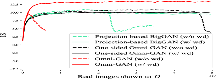
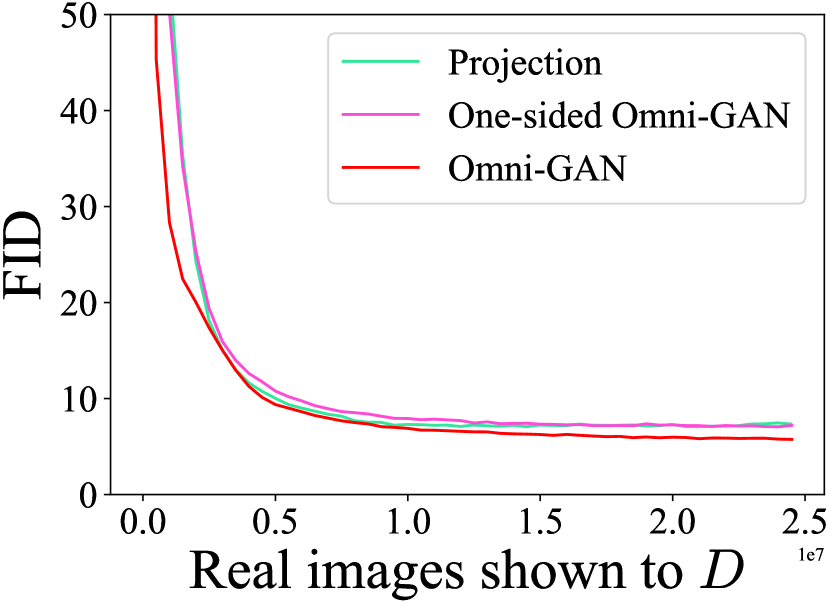
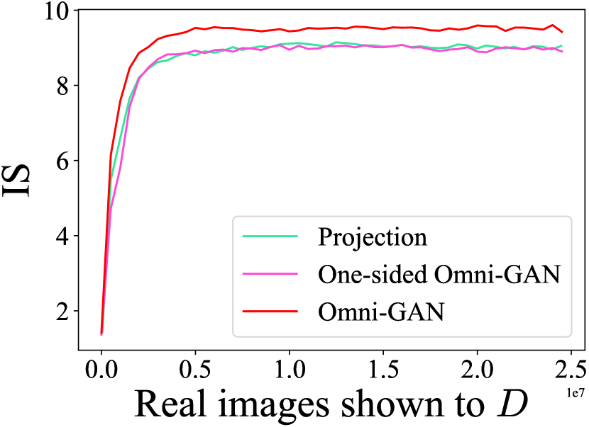
We conducted control experiments on CIFAR100 [35], and compared Omni-GAN and one-sided Omni-GAN with a projection-based cGAN, namely BigGAN [6]. As shown in Fig. 3, One-sided Omni-GAN is on par with BigGAN in terms of IS, indicating that one-sided Omni-GAN is indeed a projection-based cGAN. We can see from Eq. (11), (12) and (13) that one-sided Omni-GAN does not make full use of the class label’s supervision. Those elements with label in the output vector of the discriminator are ignored (i.e., they are not used to calculate the omni-loss, meaning these elements will not get gradients when backpropagation). Therefore, we think that the projection-based cGAN is an implicit and weaker cGAN in the sense that it does not make full use of the supervision of the class label.
On the other hand, as a classification-based cGAN, Omni-GAN makes full use of class supervision (strong supervision). However, it suffers a severe collapse in the initial stages of training. As shown in Fig. 3, the IS of Omni-GAN shows a significant upward compared to the projection-based cGAN but drops dramatically when about M real images ( epoch) are shown to the discriminator.
Our core discovery is that a moderate regularization effectively prevents the early collapse of classification-based cGANs. In practice, we use weight decay [36] as the choice of regularization. We call weight decay moderate regularization in that it does not introduce considerable computational overhead as other regularizations do, such as gradient penalty [21, 42, 74]. Therefore, Omni-GAN can be trained efficiently on large-scale datasets such as ImageNet. As shown in Fig. 3, combined with weight decay, Omni-GAN has greatly improved its IS compared to BigGAN. Moreover, we observe the projection-based cGAN, BigGAN, also collapses after long training. Weight decay is also effective for alleviating the collapse of BigGAN.
Note that we are not the first to use weight decay in GANs. [81] applys weight decay to unconditional GANs. However, our main contribution is to emphasize that the combination of strong supervision and weight decay is the key to cGANs. In fact, combining weight decay with weakly supervised cGANs even hurts performance. As shown in Fig. 3, both projection-based BigGAN and one-sided Omni-GAN suffer performance degradation after combined with weight decay.
In summary, we claim that the combination of strong supervision and weight decay is critical for cGANs. Strong supervision helps boost the performance of cGANs but causes severe early collapse. Weight decay effectively alleviates early collapse, so that cGANs can fully enjoy the benefits of strong supervision.
3.3 Comparison to Previous Approaches
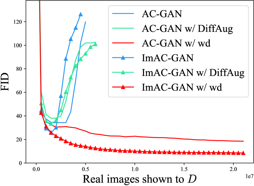
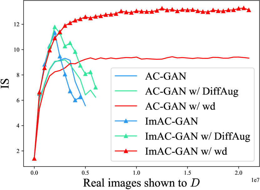
We study another well-known classification-based cGAN, AC-GAN [49], and show its results in Fig. 4. AC-GAN also suffers severe early collapse like Omni-GAN does. One possible explanation for the early collapse of classification-based cGANs is that the discriminator overfits the training data [31]. Therefore, we study whether data augmentation is effective to alleviate the early collapse. As shown in Fig. 4, AC-GAN combined with differentiable data augmentation (DiffAug) [79]222We did not choose ADA augmentation because ADA needs to design different overfitting heuristics for different losses. still cannot avoid early collapse. However, weight decay is still very effective in alleviating the early collapse of AC-GAN.
We emphasize that weight decay prevents overfitting of the discriminator at the model level, and data augmentation does at the data level. We will show in experiments that both methods are effective for improving the performance of cGANs. However, we empirically find that weight decay is almost effective in preventing the early collapse of classification-based cGANs, but data augmentation is not always effective.
Next, we investigate whether spectral normalization (SN) [46] and gradient penalty [21, 42, 74] will alleviate early collapse. Because the network architectures of the generator and discriminator we used in our experiments employ SN by default, Omni-GAN and AC-GAN still suffer severe early collapse, indicating that SN cannot alleviate the collapse problem of classification-based cGANs. In addition, we have empirically found that gradient penalty cannot help classification-based cGANs avoid early collapse (refer to Appendix B for experimental results).
Finally, by comparing AC-GAN and Omni-GAN’s loss functions, we found that the original AC-GAN still has room for improvement. Due to space limitations, we put the details in Appendix C. We name the improved AC-GAN ImAC-GAN. As shown in Fig. 4, the performance of ImAC-GAN is significantly better than that of AC-GAN, and is comparable to that of Omni-GAN (refer to Sec. 4.1).
To sum up, our results reveals that fully utilizing the supervision can improve performance of cGANs, but at the risk of early collapse. This work offers a practical way (weight decay) to overcome the collapse issue, so that the trained model enjoys both superior performance and safe optimization.
 |
 |
 |
 |
 |
 |
| (a) Grayscale image | (b) Autocolorize [37] | (c) Zhang et al. [78] | (d) Restored image (DGP w/ BigGAN) | (e) Restored image (DGP w/ Omni-INR-GAN) | (f) Ground truth |
3.4 Omni-INR-GAN: Being Friendly to Downstream Tasks
Omni-GAN is easily implemented and freely integrated with off-the-shelf encoding methods. We derive Omni-INR-GAN by integrating implicit neural representation (INR) [51, 44, 11] into Omni-GAN. Omni-INR-GAN employs INR to enhance the generator’s output layer. Due to limited space, we detail technical details in Appendix D.
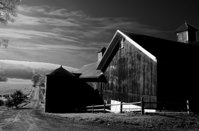
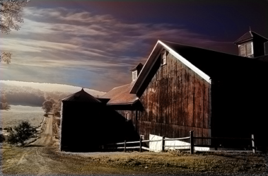
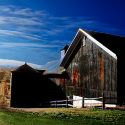
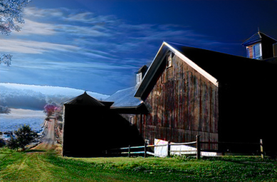
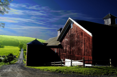
Omni-INR-GAN has the ability to output images with any aspect ratio and any resolution. Thus it is friendly to downstream tasks like image restoration. Fig. 5 shows an example of combining Omni-INR-GAN with DGP [50] for colorization. As shown in Fig. 5 (d), the DGP with BigGAN model only colorize a square patch in the original image. This is because BigGAN only generates fixed-size images, which is inflexible for downstream tasks. On the other hand, Omni-INR-GAN is able to generate images with any aspect ratio and any resolution easily so as to directly handle the entire degraded image. Because the generator has seen considerable numbers of natural images, it owns a wealth of prior knowledge. As shown in Fig. 5 (e), utilizing the generator prior helps get a plausible color image.
Another benefit is that just adding a simple INR network, whose parameters can be neglected compared to the backbone of the generator, greatly boost Omni-GAN’s performance on ImageNet. For example, Omni-INR-GAN improves the IS of Omni-GAN from to on ImageNet , and from to on ImageNet , respectively (refer to experiments for details).
4 Experiments
| No. | Method | CIFAR10 | CIFAR100 | ||||
| FID | IS | Collapse? | FID | IS | Collapse? | ||
| - | FQ-GAN [80] | No | No | ||||
| - | Multi-hinge [34] | No | Yes | ||||
| - | ADA [31] | - | - | - | - | ||
| 0 | BigGAN, wd [6] | Yes | Yes | ||||
| 1 | BigGAN, wd | No | No | ||||
| 2 | BigGAN, DiffAug, wd | No | No | ||||
| 3 | BigGAN, DiffAug, wd | No | No | ||||
| 4 | AC-GAN, wd [49] | Yes | Yes | ||||
| 5 | AC-GAN, wd | No | No | ||||
| 6 | AC-GAN, DiffAug, wd | No | Yes | ||||
| 7 | AC-GAN, DiffAug, wd | No | No | ||||
| 8 | ImAC-GAN, wd | Yes | Yes | ||||
| 9 | ImAC-GAN, wd | No | No | ||||
| 10 | ImAC-GAN, DiffAug, wd | No | Yes | ||||
| 11 | ImAC-GAN, DiffAug, wd | No | No | ||||
| 12 | Omni-GAN, wd | Yes | Yes | ||||
| 13 | Omni-GAN, wd | No | No | ||||
| 14 | Omni-GAN, DiffAug, wd | No | Yes | ||||
| 15 | Omni-GAN, DiffAug, wd | 10.37 | No | 15.37 | No | ||
| 16 | Omni-INR-GAN, wd | Yes | Yes | ||||
| 17 | Omni-INR-GAN, wd | No | No | ||||
| 18 | Omni-INR-GAN, DiffAug, wd | Yes | Yes | ||||
| 19 | Omni-INR-GAN, DiffAug, wd | No | 6.70 | No | |||
| Method | ImageNet | ImageNet | ||||||
| FID (train) | FID (val) | IS | G Params | FID (train) | FID (val) | IS | G Params | |
| CR-BigGAN† [77] | - | - | - | - | - | - | - | |
| S3GAN† [40] | - | - | - | - | - | - | ||
| BigGAN‡ [6] | M | - | - | - | - | |||
| BigGAN⋆ | M | M | ||||||
| Omni-GAN | M | M | ||||||
| Omni-INR-GAN | M | M | ||||||
4.1 Evaluation on CIFAR
We compare a projection-based cGAN, BigGAN, and several classification-based cGANs, including AC-GAN, ImAC-GAN, Omni-GAN, and Omni-INR-GAN. We also study the effects of data augmentation and weight decay on these methods. Results are summarized in Table 1.
First, let us focus on the projection-based cGAN, BigGAN. We found that data augmentation helps improve the performance of BigGAN, but weight decay cannot, even being harmful. This is reasonable because BigGAN belongs to projection-based cGANs, whose discriminator is essentially a weak implicit classifier. Weight decay constrains the fitting ability of the discriminator (i.e., a weak network). Moreover, the supervision for the discriminator is too weak (i.e., a weak supervision). As such, the performance is naturally not good.
Next, we compare AC-GAN and ImAC-GAN, which belong to classification-based cGANs. ImAC-GAN has a clear and consistent improvement over AC-GAN in all experiments. This improvement is achieved by slightly modifying the loss function of AC-GAN to be consistent with Omni-GAN (refer to Appendix C for technical details).
Third, ImAC-GAN and Omni-GAN are both superior classification-based cGANs, and their performance is comparable. ImAC-GAN uses cross-entropy as the classification loss, so it only supports single-label classification. However, the omni-loss used by Omni-GAN naturally supports multi-label classification. Therefore when the image owns multiple positive labels, Omni-GAN is more flexible than ImAC-GAN. We give an example of using Omni-GAN to generate images with multiple positive labels in Appendix E.
We find that training collapse is more likely to appear on CIFAR100 that owns more classes. For example, all classification-based cGANs, including AC-GAN, ImAC-GAN, Omni-GAN, and Omni-INR-GAN, collapsed on CIFAR100 (shown in Table 1, No. #4, #8, #12, #16). Even if equipped with data augmentation, they still collapsed (No. #6, #10, #14, #18). However, weight decay effectively alleviates the training collapse of these methods. On CIFAR10, data augmentation can alleviate the collapse issue of classification-based cGANs (No. #6, #10, #14). We think a possible reason is that CIFAR10 has a relatively small number of categories, and each category has training images. Combining with data augmentation can effectively prevent the discriminator from overfitting the training data. An anomaly is that data augmentation cannot prevent the collapse of Omni-INR-GAN on CIFAR10 (#18). We found in our experiments that data augmentation seems to be somewhat exclusive with Omni-INR-GAN. We guess that one possible reason is that some random shift operations in data augmentation destroy some prior information to be learned by Omni-INR-GAN from the coordinates.
Last but not least, we have tried to combine Omni-GAN with the network architecture of StyleGAN2 [33], but failed. StyleGAN2 employs some technologies like equalized learning rate [30] (explicitly scales the weights at runtime) during the training process. We found that these techniques seem to conflict with weight decay, which is the key for classification-based cGANs to avoid early collapse. Combining strong classification loss with StyleGANs while avoiding early collapse needs further exploration.
4.2 Evaluation on ImageNet
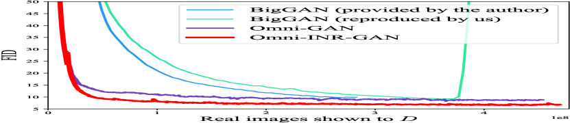
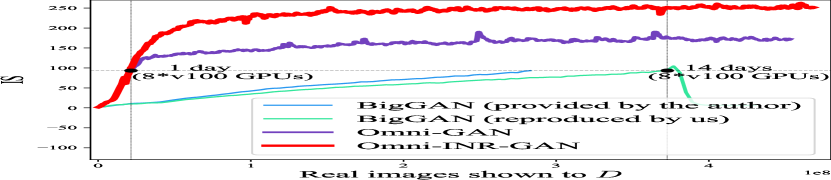
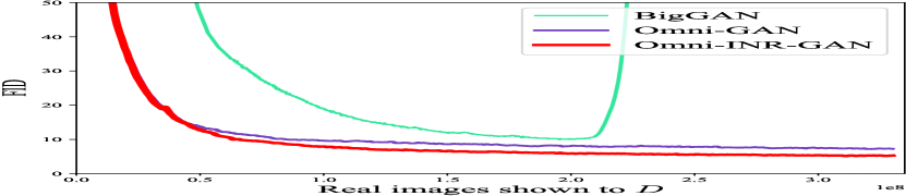
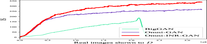
ImageNet [15] is a large dataset with number of classes and approximate M training data. We trained BigGAN333https://github.com/ajbrock/BigGAN-PyTorch., Omni-GAN, and Omni-INR-GAN on ImageNet and , respectively. The results are shown in Table 2, and the convergence curves are shown in Fig. 6 (please refer to Appendix G for more results).
As shown in Table 2 and Fig. 6, Omni-GAN shows significant advantages over BigGAN, both in terms of convergence speed and final performance. For example, Omni-GAN only took one day to reach the IS of BigGAN trained for days on ImageNet . Besides, its IS is almost twice that of BigGAN, namely vs. .
Omni-INR-GAN consistently outperforms BigGAN and Omni-GAN. As shown in Table 2, on ImageNet , the IS of Omni-INR-GAN is times that of BigGAN. We also show the number of parameters of the generator in Table 2. The number of parameters of Omni-INR-GAN is on par with that of BigGAN and Omni-GAN, indicating that the improvement does not lie in the number of parameters. We think the possible reason is that Omni-INR-GAN introduces coordinates as input, which helps the generator learn some prior knowledge of the natural images (for example, the sky often appears in the upper part of an image, and the grass often appears in the lower part on the contrary).
In summary, the significant improvement of Omni-GAN lies in the combination of strong supervision and weight decay. Strong supervision helps boost the performance of cGANs, but it causes the training to collapse earlier. Weight decay effectively alleviates the collapse problem, so that cGANs fully enjoy the benefits from strong supervision.
4.3 Application to Image-to-Image Translation
We improve the mIoU of SPADE [52] from to by only using Omni-GAN loss and weight decay for the discriminator (please refer to Appendix H for details). We believe that the improvement comes from the improved ability of the discriminator in distinguishing different classes, so that the generator receives better guidance and thus produces images with richer semantic information.
| BigGAN | Omni-GAN | Omni-INR-GAN | |
| PSNR | |||
| SSIM |
 |
|
 |
 |
 |
 |
 |
|
 |
 |
|
 |
 |
 |
 |
 |
|
 |
| Grayscale image | Finetuning iterations | Restored image | Ground truth | |||||
 |
 |

|
 |
 |
| Size () | Size () | () | () | () |
| (a) Ground truth | (b) Input | (c) LIIF | ||
 |
 |

|
 |
 |
| () | () | () | () | () |
| (d) DIP | (e) DGP w/ BigGAN | (f) DGP w/ Omni-INR-GAN (ours) | ||
4.4 Application to Downstream Tasks
Colorization. Fig. 7 shows an example of using the pre-trained BigGAN and Omni-INR-GAN to colorize images, respectively. See Appendix I for technical details. Omni-INR-GAN directly colorizes the entire image because it has the ability to output images of any resolution. However, BigGAN cannot do this. Another interesting phenomenon is that Omni-INR-GAN gradually overlays colors on the corresponding objects, indicating that the finetuning process is mining GAN’s prior information.
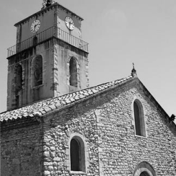
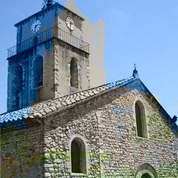
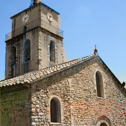
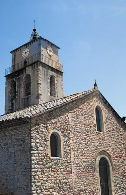
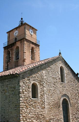
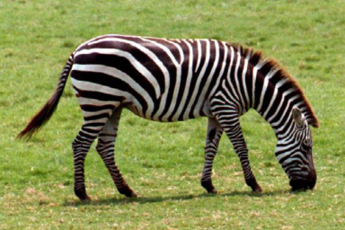
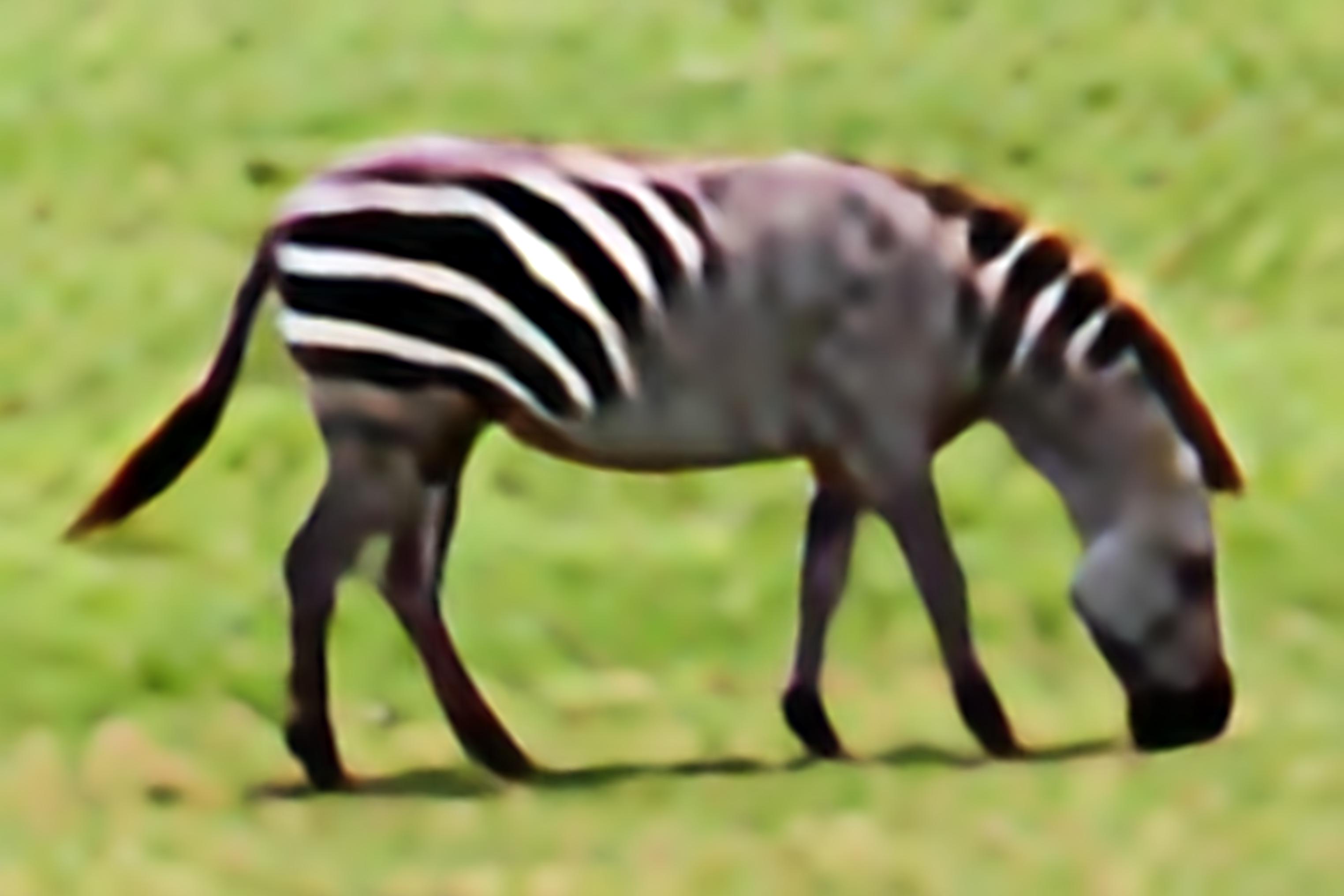
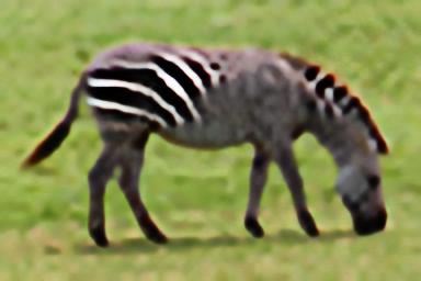
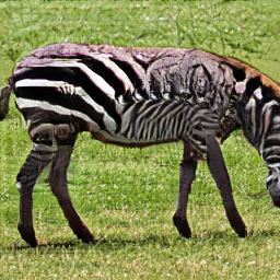
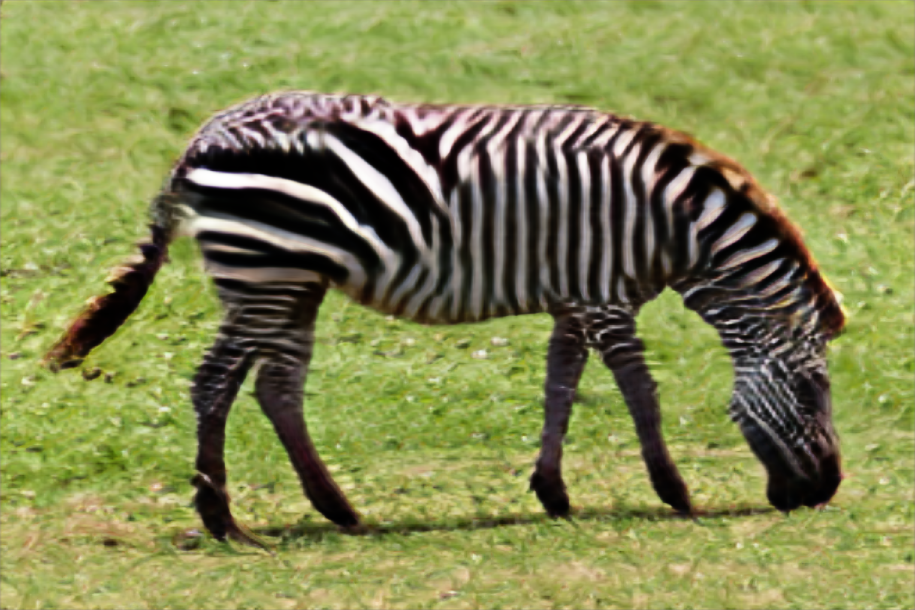
Prior Enhanced Super-Resolution Fig. 8 shows an example of using pre-trained Omni-INR-GAN for super-resolution. We deliver two messages. First, Omni-INR-GAN can extrapolate low-resolution images to any resolution. Fig. 8 (f) shows the results with upsampling scales of , , and even . Second, Omni-INR-GAN has a wealth of prior knowledge, which helps complement the missing semantics of the input. For example, for the extremely low-resolution zebra image shown in Fig. 8 (b), the image details are severely missing. In this case, although LIIF [10] has the ability to up-sample images at any scale, it cannot fill in the missing stripes of the zebra, as shown in Fig. 8 (c).
In Fig. 8 (d), DIP [71] also fails. DIP only leverages the input image and the structure of a ConvNet as the image prior. It cannot work when the input image’s resolution is too low. DGP [50] with BigGAN can only handle fixed-size images, limiting its practical application (Fig. 8 (e)). However, DGP with Omni-INR-GAN can super-resolve the entire image and extrapolate the input at any scale. In Fig. 8 (f), by mining Omni-INR-GAN’s prior, the missing zebra stripes are complemented, and a clear foreground and background are obtained. Even the shadow of the zebra is clearly visible.
5 Conclusion
This paper presents an elegant and practical solution to training effective conditional GAN models. The key discovery is that strong supervision can largely improve the upper-bound of image generation quality, but it also makes the model collapse earlier. We design the Omni-GAN algorithm that equips the classification-based loss with regularization (in particular, weight decay) to alleviate collapse. Our algorithm achieves notable performance gain in various scenarios including image generation and restoration. Our research implies that there may be more ‘secrets’ in optimizing cGAN models. We look forward to applying the proposed algorithm and pre-trained models to more scenarios and investigating further properties to improve cGAN.
References
- [1] Martin Arjovsky and Léon Bottou. Towards Principled Methods for Training Generative Adversarial Networks. arXiv:1701.04862 [cs, stat], 2017.
- [2] Martin Arjovsky, Soumith Chintala, and Léon Bottou. Wasserstein Generative Adversarial Networks. In ICML, 2017.
- [3] Matan Atzmon and Yaron Lipman. SAL: Sign Agnostic Learning of Shapes from Raw Data. arXiv:1911.10414 [cs], 2020.
- [4] David Bau, Jun-Yan Zhu, Hendrik Strobelt, Bolei Zhou, Joshua B. Tenenbaum, William T. Freeman, and Antonio Torralba. GAN Dissection: Visualizing and Understanding Generative Adversarial Networks. arXiv:1811.10597 [cs], 2018.
- [5] Mojtaba Bemana, Karol Myszkowski, Hans-Peter Seidel, and Tobias Ritschel. X-Fields: Implicit Neural View-, Light- and Time-Image Interpolation. arXiv:2010.00450 [cs], 2020.
- [6] Andrew Brock, Jeff Donahue, and Karen Simonyan. Large scale gan training for high fidelity natural image synthesis. arXiv:1809.11096, 2018.
- [7] Rohan Chabra, Jan Eric Lenssen, Eddy Ilg, Tanner Schmidt, Julian Straub, Steven Lovegrove, and Richard Newcombe. Deep Local Shapes: Learning Local SDF Priors for Detailed 3D Reconstruction. arXiv:2003.10983 [cs], 2020.
- [8] Minghao Chen, Shuai Zhao, Haifeng Liu, and Deng Cai. Adversarial-Learned Loss for Domain Adaptation. In AAAI, 2020.
- [9] Tianlong Chen, Yu Cheng, Zhe Gan, Jingjing Liu, and Zhangyang Wang. Ultra-Data-Efficient GAN Training: Drawing A Lottery Ticket First, Then Training It Toughly. arXiv:2103.00397 [cs], 2021.
- [10] Yinbo Chen, Sifei Liu, and Xiaolong Wang. Learning Continuous Image Representation with Local Implicit Image Function. arXiv:2012.09161 [cs], 2020.
- [11] Zhiqin Chen and Hao Zhang. Learning Implicit Fields for Generative Shape Modeling. arXiv:1812.02822 [cs], 2019.
- [12] Yunjey Choi, Youngjung Uh, Jaejun Yoo, and Jung-Woo Ha. StarGAN v2: Diverse Image Synthesis for Multiple Domains. In CVPR, 2020.
- [13] Marius Cordts, Mohamed Omran, Sebastian Ramos, Timo Rehfeld, Markus Enzweiler, Rodrigo Benenson, Uwe Franke, Stefan Roth, and Bernt Schiele. The Cityscapes Dataset for Semantic Urban Scene Understanding. In CVPR, 2016.
- [14] Harm de Vries, Florian Strub, Jérémie Mary, Hugo Larochelle, Olivier Pietquin, and Aaron Courville. Modulating early visual processing by language. In NeurIPS, 2017.
- [15] Jia Deng, Wei Dong, Richard Socher, Li-Jia Li, Kai Li, and Li Fei-Fei. ImageNet: A large-scale hierarchical image database. In CVPR, Miami, FL, 2009.
- [16] Emily Denton, Soumith Chintala, Arthur Szlam, and Rob Fergus. Deep Generative Image Models using a Laplacian Pyramid of Adversarial Networks. arXiv:1506.05751 [cs], 2015.
- [17] Vincent Dumoulin, Jonathon Shlens, and Manjunath Kudlur. A Learned Representation For Artistic Style. In ICLR, 2017.
- [18] Xinyu Gong, Shiyu Chang, Yifan Jiang, and Zhangyang Wang. AutoGAN: Neural Architecture Search for Generative Adversarial Networks. In ICCV, 2019.
- [19] Ian Goodfellow, Jean Pouget-Abadie, Mehdi Mirza, Bing Xu, David Warde-Farley, Sherjil Ozair, Aaron Courville, and Yoshua Bengio. Generative Adversarial Nets. In NeurIPS, 2014.
- [20] Amos Gropp, Lior Yariv, Niv Haim, Matan Atzmon, and Yaron Lipman. Implicit Geometric Regularization for Learning Shapes. arXiv:2002.10099 [cs, stat], 2020.
- [21] Ishaan Gulrajani, Faruk Ahmed, Martin Arjovsky, Vincent Dumoulin, and Aaron C Courville. Improved training of wasserstein gans. In NeurIPS, 2017.
- [22] Martin Heusel, Hubert Ramsauer, Thomas Unterthiner, Bernhard Nessler, and Sepp Hochreiter. GANs Trained by a Two Time-Scale Update Rule Converge to a Local Nash Equilibrium. In NeurIPS, 2017.
- [23] Xun Huang and Serge Belongie. Arbitrary Style Transfer in Real-time with Adaptive Instance Normalization. In ICCV, 2017.
- [24] Phillip Isola, Jun-Yan Zhu, Tinghui Zhou, and Alexei A. Efros. Image-to-Image Translation with Conditional Adversarial Networks. In CVPR, 2017.
- [25] Chiyu Max Jiang, Avneesh Sud, Ameesh Makadia, Jingwei Huang, Matthias Nießner, and Thomas Funkhouser. Local Implicit Grid Representations for 3D Scenes. arXiv:2003.08981 [cs], 2020.
- [26] Xiang Jiang, Qicheng Lao, Stan Matwin, and Mohammad Havaei. Implicit Class-Conditioned Domain Alignment for Unsupervised Domain Adaptation. In ICML, 2020.
- [27] Alexia Jolicoeur-Martineau. The relativistic discriminator: A key element missing from standard GAN. In ICLR, 2019.
- [28] Minguk Kang and Jaesik Park. ContraGAN: Contrastive learning for conditional image generation. In NeurIPS, 2020.
- [29] Animesh Karnewar and Oliver Wang. MSG-GAN: Multi-Scale Gradient GAN for Stable Image Synthesis. arXiv:1903.06048 [cs, stat], 2019.
- [30] Tero Karras, Timo Aila, Samuli Laine, and Jaakko Lehtinen. Progressive Growing of GANs for Improved Quality, Stability, and Variation. arXiv:1710.10196 [cs, stat], 2017.
- [31] Tero Karras, Miika Aittala, Janne Hellsten, Samuli Laine, Jaakko Lehtinen, and Timo Aila. Training Generative Adversarial Networks with Limited Data. arXiv:2006.06676 [cs, stat], 2020.
- [32] Tero Karras, Samuli Laine, and Timo Aila. A Style-Based Generator Architecture for Generative Adversarial Networks. In CVPR, 2019.
- [33] Tero Karras, Samuli Laine, Miika Aittala, Janne Hellsten, Jaakko Lehtinen, and Timo Aila. Analyzing and Improving the Image Quality of StyleGAN. arXiv:1912.04958 [cs, eess, stat], 2019.
- [34] Ilya Kavalerov, Wojciech Czaja, and Rama Chellappa. cGANs with Multi-Hinge Loss. arXiv:1912.04216 [cs, stat], 2019.
- [35] Alex Krizhevsky, Geoffrey Hinton, et al. Learning multiple layers of features from tiny images. Technical report, Citeseer, 2009.
- [36] Anders Krogh and John A. Hertz. A Simple Weight Decay Can Improve Generalization. In NeurIPS, 1992.
- [37] Gustav Larsson, Michael Maire, and Gregory Shakhnarovich. Learning Representations for Automatic Colorization. In ECCV, 2016.
- [38] Yann LeCun, Léon Bottou, Yoshua Bengio, Patrick Haffner, et al. Gradient-based learning applied to document recognition. Proceedings of the IEEE, 86(11), 1998.
- [39] Mingsheng Long, Zhangjie Cao, Jianmin Wang, and Michael I. Jordan. Conditional Adversarial Domain Adaptation. In NeurIPS, 2018.
- [40] Mario Lucic, Michael Tschannen, Marvin Ritter, Xiaohua Zhai, Olivier Bachem, and Sylvain Gelly. High-Fidelity Image Generation With Fewer Labels. arXiv:1903.02271 [cs, stat], 2019.
- [41] Xudong Mao, Qing Li, Haoran Xie, Raymond Y. K. Lau, Zhen Wang, and Stephen Paul Smolley. Least Squares Generative Adversarial Networks. arXiv:1611.04076 [cs], 2016.
- [42] Lars Mescheder, Andreas Geiger, and Sebastian Nowozin. Which training methods for GANs do actually Converge? In ICML, 2018.
- [43] Lars Mescheder, Sebastian Nowozin, and Andreas Geiger. The Numerics of GANs. In NeurIPS, 2017.
- [44] Lars Mescheder, Michael Oechsle, Michael Niemeyer, Sebastian Nowozin, and Andreas Geiger. Occupancy Networks: Learning 3D Reconstruction in Function Space. arXiv:1812.03828 [cs], 2019.
- [45] Mehdi Mirza and Simon Osindero. Conditional Generative Adversarial Nets. arXiv:1411.1784 [cs, stat], 2014.
- [46] Takeru Miyato, Toshiki Kataoka, Masanori Koyama, and Yuichi Yoshida. Spectral Normalization for Generative Adversarial Networks. arXiv:1802.05957 [cs, stat], 2018.
- [47] Takeru Miyato and Masanori Koyama. cGANs with Projection Discriminator. In ICLR, 2018.
- [48] Yuval Netzer, Tao Wang, Adam Coates, Alessandro Bissacco, Bo Wu, and Andrew Y Ng. Reading digits in natural images with unsupervised feature learning. 2011.
- [49] Augustus Odena, Christopher Olah, and Jonathon Shlens. Conditional Image Synthesis With Auxiliary Classifier GANs. arXiv:1610.09585 [cs, stat], 2017.
- [50] Xingang Pan, Xiaohang Zhan, Bo Dai, Dahua Lin, Chen Change Loy, and Ping Luo. Exploiting Deep Generative Prior for Versatile Image Restoration and Manipulation. In ECCV, 2020.
- [51] Jeong Joon Park, Peter Florence, Julian Straub, Richard Newcombe, and Steven Lovegrove. DeepSDF: Learning Continuous Signed Distance Functions for Shape Representation. arXiv:1901.05103 [cs], 2019.
- [52] Taesung Park, Ming-Yu Liu, Ting-Chun Wang, and Jun-Yan Zhu. Semantic Image Synthesis with Spatially-Adaptive Normalization. In CVPR, 2019.
- [53] Songyou Peng, Michael Niemeyer, Lars Mescheder, Marc Pollefeys, and Andreas Geiger. Convolutional Occupancy Networks. arXiv:2003.04618 [cs], 2020.
- [54] Guim Perarnau, Joost van de Weijer, Bogdan Raducanu, and Jose M. Álvarez. Invertible Conditional GANs for image editing. arXiv:1611.06355 [cs], 2016.
- [55] Guo-Jun Qi. Loss-Sensitive Generative Adversarial Networks on Lipschitz Densities. arXiv:1701.06264 [cs], 2017.
- [56] Xiaojuan Qi, Qifeng Chen, Jiaya Jia, and Vladlen Koltun. Semi-parametric Image Synthesis. In CVPR, 2018.
- [57] Scott Reed, Zeynep Akata, Xinchen Yan, Lajanugen Logeswaran, Bernt Schiele, and Honglak Lee. Generative Adversarial Text to Image Synthesis. In ICML, 2016.
- [58] Kevin Roth, Aurelien Lucchi, Sebastian Nowozin, and Thomas Hofmann. Stabilizing Training of Generative Adversarial Networks through Regularization. In NeurIPS, 2017.
- [59] Masaki Saito, Eiichi Matsumoto, and Shunta Saito. Temporal Generative Adversarial Nets with Singular Value Clipping. In ICCV, 2017.
- [60] Tim Salimans, Ian Goodfellow, Wojciech Zaremba, Vicki Cheung, Alec Radford, Xi Chen, and Xi Chen. Improved Techniques for Training GANs. In NeurIPS, 2016.
- [61] Edgar Schönfeld, Bernt Schiele, and Anna Khoreva. A U-Net Based Discriminator for Generative Adversarial Networks. In CVPR, 2020.
- [62] Florian Schroff, Dmitry Kalenichenko, and James Philbin. FaceNet: A Unified Embedding for Face Recognition and Clustering. In CVPR, 2015.
- [63] Woohyeon Shim and Minsu Cho. CircleGAN: Generative Adversarial Learning across Spherical Circles. 2020.
- [64] Vincent Sitzmann, Julien N. P. Martel, Alexander W. Bergman, David B. Lindell, and Gordon Wetzstein. Implicit Neural Representations with Periodic Activation Functions. In NeurIPS, 2020.
- [65] Ivan Skorokhodov, Savva Ignatyev, and Mohamed Elhoseiny. Adversarial Generation of Continuous Images. arXiv:2011.12026 [cs], 2020.
- [66] Kenneth O. Stanley. Compositional pattern producing networks: A novel abstraction of development. Genetic Programming and Evolvable Machines, 8(2), 2007.
- [67] Jianlin Su. Extending Cross-Entropy of Softmax to Multi-Label Classification. https://kexue.fm/archives/7359, 2020.
- [68] Yifan Sun, Changmao Cheng, Yuhan Zhang, Chi Zhang, Liang Zheng, Zhongdao Wang, and Yichen Wei. Circle Loss: A Unified Perspective of Pair Similarity Optimization. In CVPR, 2020.
- [69] Yuesong Tian, Li Shen, Li Shen, Guinan Su, Zhifeng Li, and Wei Liu. AlphaGAN: Fully Differentiable Architecture Search for Generative Adversarial Networks. arXiv:2006.09134 [cs, eess], 2020.
- [70] Eric Tzeng, Judy Hoffman, Kate Saenko, and Trevor Darrell. Adversarial Discriminative Domain Adaptation. arXiv:1702.05464 [cs], 2017.
- [71] Dmitry Ulyanov, Andrea Vedaldi, and Victor Lempitsky. Deep Image Prior. arXiv:1711.10925 [cs, stat], 2018.
- [72] Ting-Chun Wang, Ming-Yu Liu, Jun-Yan Zhu, Guilin Liu, Andrew Tao, Jan Kautz, and Bryan Catanzaro. Video-to-Video Synthesis. In NeurIPS, 2018.
- [73] Ting-Chun Wang, Ming-Yu Liu, Jun-Yan Zhu, Andrew Tao, Jan Kautz, and Bryan Catanzaro. High-Resolution Image Synthesis and Semantic Manipulation with Conditional GANs. In CVPR, 2018.
- [74] Jiqing Wu, Zhiwu Huang, Janine Thoma, Dinesh Acharya, and Luc Van Gool. Wasserstein divergence for gans. In ECCV, 2018.
- [75] Fisher Yu, Vladlen Koltun, and Thomas Funkhouser. Dilated Residual Networks. In CVPR, Honolulu, HI, 2017.
- [76] Han Zhang, Tao Xu, Hongsheng Li, Shaoting Zhang, Xiaogang Wang, Xiaolei Huang, and Dimitris Metaxas. StackGAN: Text to Photo-realistic Image Synthesis with Stacked Generative Adversarial Networks. In ICCV, 2017.
- [77] Han Zhang, Zizhao Zhang, Augustus Odena, and Honglak Lee. Consistency Regularization for Generative Adversarial Networks. arXiv:1910.12027 [cs, stat], 2020.
- [78] Richard Zhang, Phillip Isola, and Alexei A. Efros. Colorful Image Colorization. arXiv:1603.08511 [cs], 2016.
- [79] Shengyu Zhao, Zhijian Liu, Ji Lin, Jun-Yan Zhu, and Song Han. Differentiable Augmentation for Data-Efficient GAN Training. arXiv:2006.10738 [cs], 2020.
- [80] Yang Zhao, Chunyuan Li, Ping Yu, Jianfeng Gao, and Changyou Chen. Feature Quantization Improves GAN Training. arXiv:2004.02088 [cs, stat], 2020.
- [81] Brady Zhou and Philipp Krähenbühl. Don’t let your Discriminator be fooled. In International Conference on Learning Representations, 2018.
- [82] Peng Zhou, Lingxi Xie, Xiaopeng Zhang, Bingbing Ni, and Qi Tian. Searching towards Class-Aware Generators for Conditional Generative Adversarial Networks. arXiv:2006.14208 [cs], 2020.
Omni-GAN and Omni-INR-GAN
Supplementary Material
Appendix A Derivation from Unified Loss to Omni-loss.
A.1 Derivation of Omni-loss
The unified loss [68] is defined as
|
|
(14) |
where stands for a scale factor, and for a margin between positive and negative scores. and denote positive score set and negative score set, respectively. Eq. (14) aims to maximize and to minimize .
The omni-loss is defined as
|
|
(15) |
where is a set consisting of indexes of negative scores (), and consists of indexes of positive scores ().
Eq. (15) is a special case of Eq. (14), which has been proved by [67]. For the convenience of readers in the English community, we provide our proof here. Let be and be , then
| (16) | ||||
where means .
A.2 Gradient Analysis
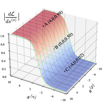
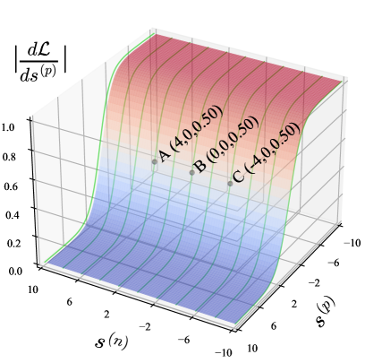
The gradients of omni-loss have two properties: on one hand, the gradients w.r.t. and are independent; on the other hand, the gradients w.r.t. (or ), , are automatically balanced. To illustrate these properties, we visualize the gradients of omni-loss. Fig. 9a shows a case that only contains one and one . , , and have the same , which is , but different (i.e., , respectively). As a result, the gradients w.r.t. at these three points are the same (i.e., ). Nevertheless, the gradients w.r.t. at these three points are different. For example, the gradient w.r.t. at is largest (equal to ). The reason for this is that the objective of omni-loss is to minimize . Thus the larger the , the larger the gradient w.r.t. .
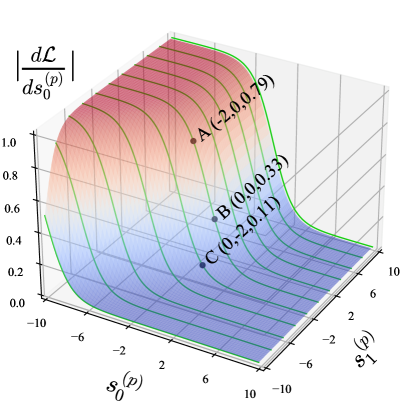
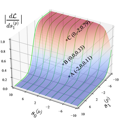
In Fig. 9b, we show the ability of omni-loss to automatically balance gradients. We consider a case with only two positive labels, namely and . We can observe that for , its is smaller than (i.e., -2 vs. 0). As a result, the gradients w.r.t. is larger than that w.r.t. (i.e., 0.79 vs. 0.11), meaning that the omni-loss try to increase with higher superiority. A similar analysis applies to as well. For , since and are equal, the gradients of them are also equal ().
Appendix B Gradient Penalty for Classification-based cGANs
We investigate whether gradient penalty will alleviate early collapse. We chose AC-GAN [49], the currently widely known classification-based cGAN, as the testbed, and evaluate three gradient penalty methods: WGAN-GP [21], WGAN-div [42], and R1 regularization [74]. Because cGANs are more likely to collapse when the number of categories is large, we evaluate them on CIFAR100 instead of CIFAR10. As shown in Fig. 10, none of the three gradient penalty methods can prevent AC-GAN from collapsing. We emphasize that computing gradient penalties will introduce additional computational overhead during GAN’s training, which is very unfriendly to large-scale datasets such as ImageNet. However, weight decay effectively alleviates the collapse problem without adding any additional training overhead.
Appendix C Improved AC-GAN (ImAC-GAN)
Auxiliary classifier GAN (AC-GAN) [49] uses an auxiliary classifier to enhance the standard GAN model. Its objective function consists of tow parts: the GAN loss, , and the classification loss, :
| (21) | ||||
| (22) |
where g is a random variable denoting the class label and is the ground truth label of . and represent a real image and a generated image respectively. The discriminator of AC-GAN is trained to maximize , and the generator is trained to maximize .
The discriminator loss of AC-GAN is not optimal. We give a slightly modified version below. Suppose the dataset owns categories, then the discriminator is trained to maximize
| (23) | ||||
where is the ground truth class label of , and means that belongs to the fake class. To sum up, we use an additional class to represent the generated image. In practice, this is achieved by setting the dimension of the fully connected layer of the auxiliary classification layer to be rather than .
The objective function of the generator is consistent with that of the original AC-GAN, i.e., maximizing
| (24) |
where is the class label used by the generator to generate .
We name this improved version of AC-GAN ImAC-GAN. As shown in the paper, ImAC-GAN is comparable to Omni-GAN, both of which achieve superior performance compared to projection-based cGANs. However, because ImAC-GAN uses cross-entropy as the loss function for classification, it can only handle the case where the sample has a positive label. Omni-GAN uses omni-loss, essentially a multi-label classification loss, which naturally supports handling samples with one positive label or multiple positive labels. We will give an example of generating images with multiple positive labels in Sec. E.
Appendix D Technical Details of Omni-INR-GAN
Learning image prior model is helpful for image restoration and manipulation, such as denoising, inpainting, and harmonizing. Deep generative prior (DGP) [50] showed the potential of employing the generator prior captured by a pre-trained GAN model (i.e., a BigGAN model trained on a large-scale image dataset, ImageNet). However, BigGAN can only output images with a fixed aspect ratio, limiting the practical application of DGP. To make the pre-trained GAN model more flexible for downstream tasks, we propose a new GAN named Omni-INR-GAN, which can output images with any aspect ratio and any resolution.
Images are usually represented by a set of pixels with fixed resolution. A popular method named implicit neural representation (INR) is prevalent in the 3D field [51, 44, 11]. Recently, people introduced the INR method to 2D images [10, 65]. As shown in Fig. 11 (a), the INR of an image directly maps (, ) coordinates to image’s RGB pixel values. Since the coordinates are continuous, once we get the INR of an image, we can get images of arbitrary resolutions by sampling different numbers of coordinates.
Inspired by the local implicit image function (LIIF) [10], we use INR to enhance Omni-GAN, with the goal of enabling the generator to output images with any aspect ratios and any resolution. We name our method Omni-INR-GAN. As shown in Fig. 11 (b), we keep the backbone of the generator network unchanged and employ an INR network for the output layer. Let represent the output feature map of the backbone, be the implicit neural function. Then the RGB signal at (, ) coordinate is given by , where stands for the feature vector at (, ). Note that since and can be any real numbers, may not exist in . In such a case, we adopt the bilinear interpolation of the four feature vectors near (, ) as the feature at (, ).
Omni-INR-GAN can generate images with any aspect ratio, so as to be more friendly to downstream tasks like image restoration and manipulation. After trained on the large-scale dataset ImageNet, Omni-INR-GAN can be combined with DGP to do restoration tasks. Omni-INR-GAN eliminates cropping operations before image restoration, making it possible to repair the entire image directly. Since the generator has seen considerable natural images, utilizing the generator prior can facilitate downstream tasks significantly.
Appendix E An Example of Multi-label Discriminator
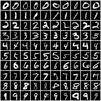
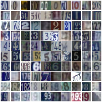
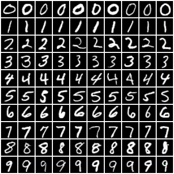
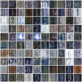
Omni-loss is essentially a multi-label classification loss and naturally supports classification with multiple positive labels. To verify the ability of Omni-GAN for generating samples with multiple positive labels, we construct a mixed dataset containing images of digits from two distinct domains, namely MNIST [38] of handwritten digits and SVHN [48] of house numbers. Some example images from the datasets are shown in Fig. 13. In this setting, the discriminator needs to predict three attributes, class (recognizing digits), domain, and reality.
Let us take images of MNIST as an example, and show how to set the loss for the discriminator. As for SVHN, the case is analogous. Suppose is an image sampled from MNIST, its multi-label vector is given by
| (25) |
where means the corresponding score belongs to the negative set, and to the positive set. As can be seen, possesses three positive labels. The multi-label vector for is then given by
| (26) |
which is a one-hot vector with the last element being . The discriminator loss is given by
| (27) | ||||
For generator, its goal is to cheat the discriminator. The multi-label vector for is given by
| (28) |
where is if its index in the vector is equal to the label adopted by the generator to generate , otherwise . The generator loss is given by.
| (29) |
We experimentally found that this multi-label discriminator can instruct the generator to generate images from different domains. Some generated images are shown in Fig. 13. We must emphasize that this is only a preliminary experiment to verify the function of the multi-label discriminator. We look forward to applying the multi-label discriminator to other tasks in the future, such as translation between images in different domains, domain adaptation, etc.
Appendix F Additional Results on CIFAR
F.1 Over-fitting of the Discriminator
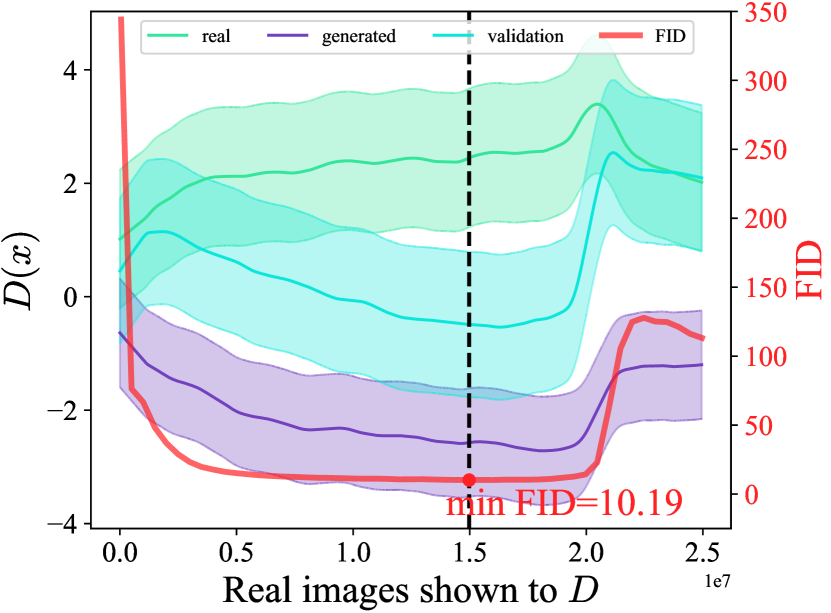
Karras et al. [31] found that the discriminator overfits the training dataset, which will lead to incorrect gradients provided to the generator. Thus the training diverges. To verify that the collapse of the projection-based cGAN is due to the over-fitting of the discriminator, we plotted the scalar output of the discriminator, , over the course of training. We utilized the test set of CIFAR100 containing images as the verification set, which was not used in the training.
As shown in Fig. 14a, obviously, as training progresses, the of the validation set tends to that of the generated images, substantiating that the discriminator overfits the training data. We also plotted the FID curve in the same figure. We can see that the training commences diverging when showing about M real images (i.e., around epoch) to the discriminator. The best FID is obtained when approximately M real images are shown to the discriminator.
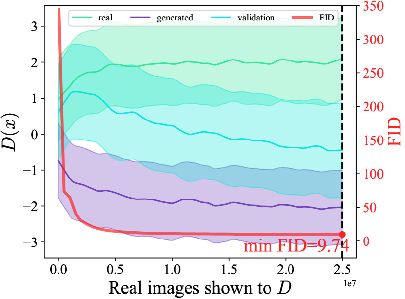
In Fig. 14b, we show the and FID after applying weight decay to the projection-based discriminator. We can find that although the discriminator still overfits the training data, the training dose not collapse during the whole training process (the minimum FID, , is reached at the end of the training).
F.2 Comparison of One-sided Omni-GAN and Projection-based GAN on CIFAR10
We provide the results of one-sided Omni-GAN and projection-based BigGAN on CIFAR10. As shown in Fig. 15, one-sided Omni-GAN is comparable to the projection-based BigGAN in terms of both FID and IS. This proves that one-sided Omni-GAN indeed belongs to projection-based cGANs. Both one-sided Omni-GAN and projection-based BigGAN are inferior to Omni-GAN. Because the only difference between one-sided Omni-GAN and Omni-GAN is whether the supervision is fully utilized, we conclude that the superiority of Omni-GAN lies in the full use of supervision.
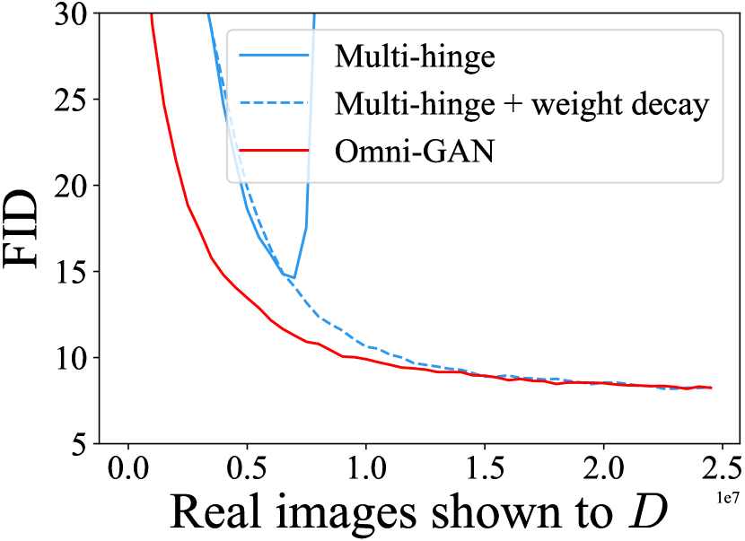
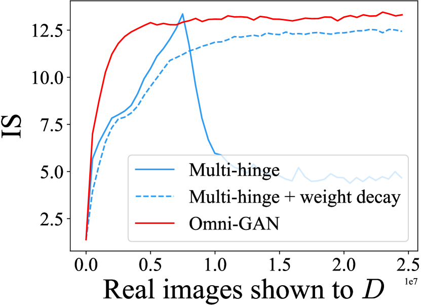
F.3 Comparison with Multi-hinge GAN
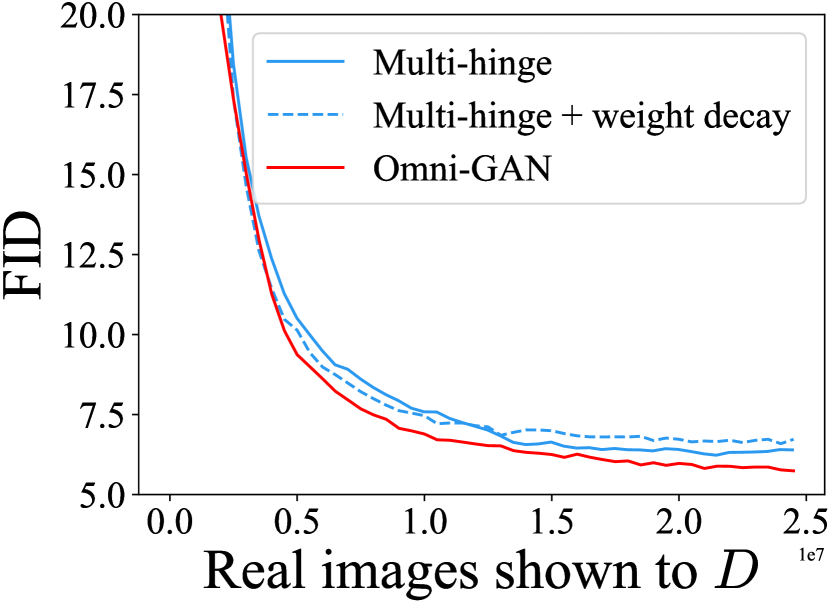
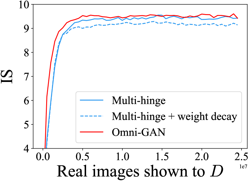
Multi-hinge GAN belongs to classification-based cGANs, and also suffers from the early collapse issue. We study whether weight decay is effective for Multi-hinge GAN. As shown in Fig. 16, original Multi-hinge GAN suffers a severe early collapse issue. After equipped with weight decay, Multi-hinge GAN enjoys a safe optimization and its FID is even comparable to that of Omni-GAN. However, its IS is worse than that of Omni-GAN.
Multi-hinge GAN combined with weight decay does not always perform well. The results on CIFAR10 are shown in Fig. 17. Weight decay deteriorates Multi-hinge GAN in terms of both FID and IS. However, Omni-GAN outperforms Multi-hinge GAN. In addition, omni-loss is more flexible than multi-hinge loss. It supports implementing a multi-label discriminator. As a result, we suggest first considering using Omni-GAN when choosing cGANs.
F.4 Applying Weight Decay to the Generator
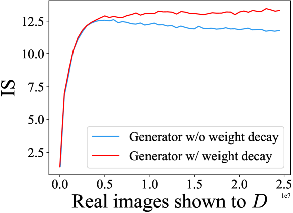
We found empirically that applying weight decay also to the generator can make training more stable. As shown in Fig. 18, although only applying weight decay to the discriminator can avoid the risk of collapse earlier, the IS has a trend of gradually decreasing as the training progresses. Fortunately, applying weight decay (set to be in our most experiments) to the generator can solve this problem. This phenomenon seems to indicate that the generator is also at a risk of over-fitting.
F.5 How to Set the Weight Decay?
We did a grid search for the weight decay on CIFAR and found that its value is related to the size of the training dataset. For CIFAR100, there are only images per class, and the weight decay is set to be . For CIFAR10, there are images per class, and the weight decay is set to be . For ImageNet, it is a large dataset with a considerable number of training data (approximate M). The weight decay is set to 0.00001. The conclusion is that the smaller the dataset, the higher the risk of over-fitting for the discriminator. Then weight decay should be larger.
Appendix G Additional Results on ImageNet
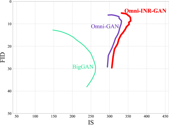
We provide convergence curves on ImageNet . As shown in Fig. 19, both Omni-GAN and Omni-INR-GAN converge faster than BigGAN, proving the effectiveness of combining strong supervision and weight decay. Omni-INR-GAN clearly outperforms Omni-GAN, showing its significant potential for future applications. In Fig. 20, we show the tradeoff curve of these methods using the truncation trick on ImageNet . Omni-INR-GAN is consistently superior to Omni-GAN and BigGAN.
Appendix H Application to Image-to-Image Translation
| SPADE [52] | road | sidewalk | building | wall | fence | pole | traffic light | traffic sign | vegetation | terrain |
| sky | person | rider | car | truck | bus | train | motorcycle | bicycle | mIoU | |
| + Omni-GAN | road | sidewalk | building | wall | fence | pole | traffic light | traffic sign | vegetation | terrain |
| sky | person | rider | car | truck | bus | train | motorcycle | bicycle | mIoU | |
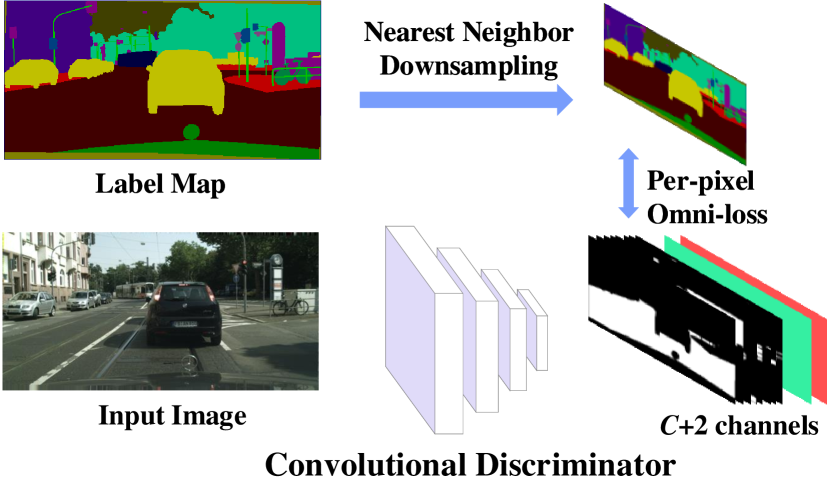
Omni-GAN can be used for image-to-image translation tasks. We verify the effectiveness of Omni-GAN on semantic image synthesis [72, 56]. In particular, we replace the GAN loss of SPADE [52] with Omni-GAN’s loss, and keep other hyper-parameters unchanged. The discriminator is a fully convolutional network, which is widely adopted by image-to-image translation tasks [52, 24, 73]. As shown in Fig. 21, the discriminator takes images as input and outputs feature maps with the number of channels being . represents the number of classes which is analogous to that of the semantic segmentation task. indicates there are two extra feature maps representing to what extent the input image is real or fake. We adopt nearest neighbor downsampling to downsample the label map to the same resolution as the output feature maps of the discriminator. Then we use the downsampled label map as the ground truth label, and apply a per-pixel omni-loss to the output feature maps of the discriminator.
We use Cityscapes dataset [13] as a testbed, and train models on the training set with size of . The images is resized to . Models are evaluated by the mIoU of the generated images on the test set with images. We use a pre-trained DRN-D-105 [75] as the segmentation model for the sake of evaluation. As shown in Table 4, Omni-GAN improves the mIoU score of SPADE from to , substantiating that the synthesized images possess more semantic information. We believe that the improvement comes from the improved ability of the discriminator in distinguishing different classes, so that the generator receives better guidance and thus produces images with richer semantic information.
Appendix I Application to Downstream Tasks
I.1 Colorization and Super-resolution
Deep generative prior (DGP) [50] showed the potential of employing image prior captured by a pre-trained GAN model. Our colorization and super-resolution schemes are based on DGP. We first introduce the preliminary knowledge of DGP.
Suppose is a natural image and is a degradation function, e.g., gray transform for colorization and down-sampling for super-resolution. Then represents the degraded image, i.e., a partial observation of the original image, . The goal of image restoration is to recover from with the help of some statistical image prior of . DGP proposes employing the image prior stored in a pre-trained GAN’s generator. The objective is defined as
| (30) |
where is a noise vector. represents the generator in GAN and is parameterized by . is a discriminator-based distance metric: . is the discriminator coupled with . is a index set for feature maps of different blocks of . Note that both and have been trained on a large-scale natural image dataset. DGP employs the prior of by fine-tuning and . After fine-tuning, we get the restored image .
Although DGP has achieved noteworthy results in image restoration and manipulation, it has limitations due to the inflexibility of the pre-trained GAN model. For example, if DGP adopts a BigGAN model, DGP must first crop the original image into image patch of size before restoration, restricting its practical application. However, because Omni-INR-GAN can output images of any resolution, combining it with DGP can directly restore the original image.
We use Omni-INR-GAN pre-trained on ImageNet for colorization and super-resolution. Eq. (30) is the objective. For colorization, is a grayscale image, and for super-resolution, is a low-resolution image. We resize the input image’s short edge to and keep the aspect ratio of the image unchanged. After fine-tuning, is the restored image. Because represents in the INR form, we can get the restored image at any resolution through . Therefore, Omni-INR-GAN is more friendly to downstream tasks.
I.2 Reconstruction
We compare pre-trained GAN models for image reconstruction tasks. Specifically, we finetune the parameters of the generator to make it reconstruct given images. Note that we do not use mse or L1 loss, because these loss functions make it easy for the generator to overfit the given image, as long as the training iterations are enough. Instead, we only use the discriminator feature loss, because it has been proven to be very effective for utilizing the prior of the generator. For the dataset, we use 1k images sampled from the ImageNet validation set, which is the same as DGP’s choice. Note that these data have not been used in GAN’s training. We adopt the progressive reconstruction strategy of DGP [50], and finetune each GAN model for the same number of iterations.
Appendix J Implementation Details
We adopt BigGAN architectures of and in our experiments. Table 5, 6, 7, and 8 show the architectural details. Each experiment is conducted on eight v100 GPUs. Training Omni-GAN on ImageNet and took days and days, respectively. Training Omni-INR-GAN on ImageNet and took days and days, respectively. No collapse occurred during the entire training process. We have found experimentally that classification-based cGANs cannot set a large batch size like projection-based BigGAN. For all experiments of Omni-GAN and Omni-INR-GAN, the batch size is set to . We adopt the ADAM optimizer in all experiments, with betas being and . The learning rates of the generator and discriminator are set to and , respectively.
For experiments, the generator and discriminator use non-local block at resolution. The generator is updated once every time the discriminator is updated. The weight decay of the generator and discriminator are set to and , respectively. For Omni-INR-GAN, we removed the non-local block at resolution of the discriminator. Because when Omni-INR-GAN is used for downstream tasks, the input image of the discriminator may be of any size, so the middle layer of the discriminator may not output resolution features. Moreover, although Omni-INR-GAN can generate images of any resolution, we did not adopt a multi-scale training strategy. We found that multi-scale training led to training collapse. We think that a possible reason is that multi-scale training enhances the discriminator, resulting in the ability of the generator and the discriminator to be out of balance. Thus we only generate images during training, and the real images are also resized to .
For experiments, the weight decay of the generator and discriminator are set to and , respectively. The generator is updated once every time the discriminator is updated twice. We have found experimentally that this will make training more stable. The generator and discriminator use non-local block at resolution rather than due to limited GPU memory. For Omni-INR-GAN, in order to support downstream tasks friendly, we do not use non-local block in the discriminator. Moreover, due to GPU memory limitation, we reduce the batch size to and accumulate the gradient twice to approximate the gradient when the batch size is . We did not adopt a multi-scale training strategy. Only images are generated during training, and the real images are also resized to .
| Linear |
| ResBlock up |
| ResBlock up |
| ResBlock up |
| ResBlock up |
| Non-local Block () |
| ResBlock up |
| BN, ReLU, Conv |
| Tanh |
| RGB image |
| ResBlock down |
| Non-local Block () |
| ResBlock down |
| ResBlock down |
| ResBlock down |
| ResBlock down |
| ResBlock |
| ReLU, global sum pooling |
| Linear |
| Linear |
| ResBlock up |
| ResBlock up |
| ResBlock up |
| ResBlock up |
| Non-local Block () |
| ResBlock up |
| ResBlock up |
| BN, ReLU, Conv |
| Tanh |
| RGB image |
| ResBlock down |
| ResBlock down |
| Non-local Block () |
| ResBlock down |
| ResBlock down |
| ResBlock down |
| ResBlock down |
| ResBlock |
| ReLU, global sum pooling |
| Linear |
| Linear |
| ResBlock up |
| ResBlock up |
| ResBlock up |
| ResBlock up |
| Non-local Block () |
| ResBlock up |
| Unfold(kernel_size=3) |
| Grid_sample(), Concat feature and |
| Linear, Relu |
| Linear, Relu |
| Linear |
| Tanh |
| RGB image |
| ResBlock down |
| ResBlock down |
| ResBlock down |
| ResBlock down |
| ResBlock down |
| ResBlock |
| ReLU, global sum pooling |
| Linear |
| Linear |
| ResBlock up |
| ResBlock up |
| ResBlock up |
| ResBlock up |
| Non-local Block () |
| ResBlock up |
| ResBlock up |
| Unfold(kernel_size=3) |
| Grid_sample(), Concat feature and |
| Linear, Relu |
| Linear, Relu |
| Linear |
| Tanh |
| RGB image |
| ResBlock down |
| ResBlock down |
| ResBlock down |
| ResBlock down |
| ResBlock down |
| ResBlock down |
| ResBlock |
| ReLU, global sum pooling |
| Linear |
Appendix K Additional Results
K.1 Generated Images on CIFAR
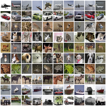
In Fig. 22 and 23, we show generated images from Omni-GAN on CIFAR10, CIFAR100 respectively. Due to limited space, we only show images of some categories on CIFAR100.
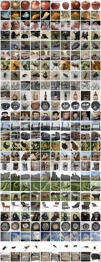
K.2 Generated Images on ImageNet
Omni-INR-GAN inherently supports generating images of arbitrary resolution. We adopt the Omni-INR-GAN model to generate some images with different resolutions, e.g., Fig. 24, 25, etc.
 |
 |
 |
 |
 |
 |
||
|
|
|
|
|
|
||
|
|
|
|
|
|
||
|
|
|
|
|
|
||
|
|
|
|
|
|
||
|
|
|
|
|
|
||
|
|
|
|
|
|
||
|
|
|
|
|
|
||
|
|
|
|
|
|
||
|
|
|
|
|
|
||
|
|
|
|
|
|
||
|
|
|
|
|
|
||
|
|
|
|
|
|
||
|
|
|
|
|
|
||
|
|
|
|
|
|
||
|
|
|
|
|
|
||
|
|
|
|
|
|
||
|
|
|
|
|
|
||
 |
 |

|
 |
 |
| Size () | Size () | () | () | () |
| (a) Ground truth | (b) Input | (c) LIIF | ||
 |
 |

|
 |
 |
| () | () | () | () | () |
| (d) DIP | (e) DGP w/ BigGAN | (f) DGP w/ Omni-INR-GAN (ours) | ||
K.3 Results of Semantic Image Synthesis
In Fig. 43, we show several results of Omni-GAN as well as those of SPADE for semantic image synthesis. The label maps and the ground truth images are from the first ten items in the test set of Cityscapes dataset, without cherry-picking.
| Label | Ground Truth | SPADE | Ours |
 |
 |
 |
 |
 |
 |
 |
 |
 |
 |
 |
 |
 |
 |
 |
 |
 |
 |
 |
 |
 |
 |
 |
 |
 |
 |
 |
 |
 |
 |
 |
 |
 |
 |
 |
 |
 |
 |
 |
 |