Early Life Cycle Software Defect Prediction.
Why? How?

Abstract

Many researchers assume that, for software analytics, “more data is better.” We write to show that, at least for learning defect predictors, this may not be true.

To demonstrate this, we analyzed hundreds of popular GitHub projects. These projects ran for 84 months and contained 3,728 commits (median values). Across these projects, most of the defects occur very early in their life cycle. Hence, defect predictors learned from the first 150 commits and four months perform just as well as anything else. This means that, at least for the projects studied here, after the first few months, we need not continually update our defect prediction models.

We hope these results inspire other researchers to adopt a “simplicity-first” approach to their work. Some domains require a complex and data-hungry analysis. But before assuming complexity, it is prudent to check the raw data looking for “short cuts” that can simplify the analysis.

I Introduction

This paper proposes a data-lite method that finds effective software defect predictors using data just from the first 4% of a project’s lifetime. Our new method is recommended since it means that we need not always revise defect prediction models, even if new data arrives. This is important since managers, educators, vendors, and researchers lose faith in methods that are always changing their conclusions.

Figure 1: 1.2 million commits for 155 GitHub projects. Black:Red (shaded) = Clean:Defective commits. In this paper, we compare (a) models learned up to the vertical green (dotted) line to (b) models learned using more data.

Our method is somewhat unusual since it takes an opposite approach to data-hungry methods that (e.g.) use data collected across many years of a software project [1, 2]. Such data-hungry methods are often cited as the key to success for data mining applications. For example, in his famous talk, “The Unreasonable Effectiveness of Data,” Google’s Chief Scientist Peter Norvig argues that “billions of trivial data points can lead to understanding” [3] (a claim he supports with numerous examples from vision research).

But what if some Software Engineering (SE) data was not like Norvig’s data? What if SE needs its own AI methods, based on what we learned about the specifics of software projects? If that were true, then data-hungry methods might be needless over-elaborations of a fundamentally simpler process.

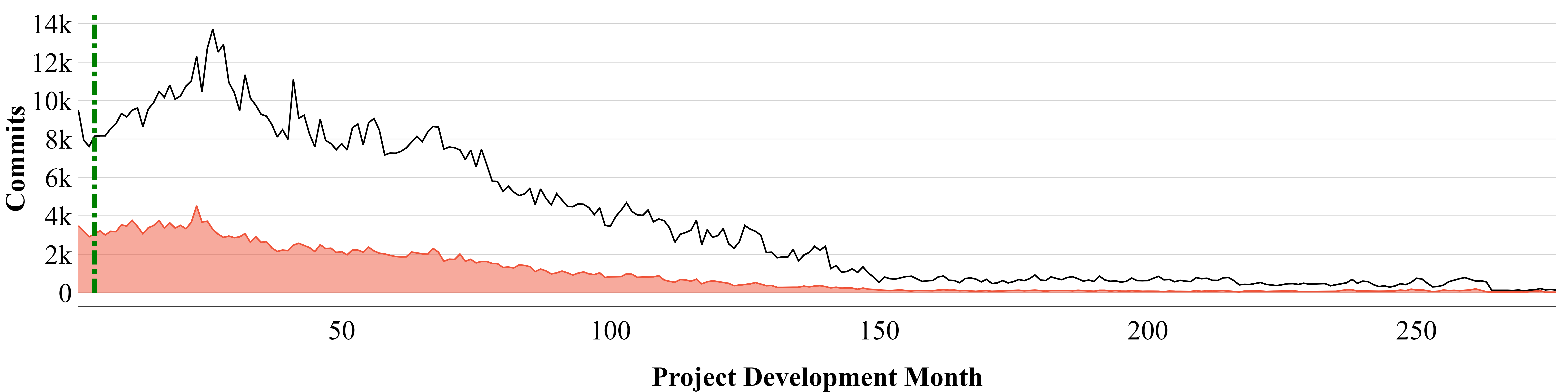
This paper shows that for one specific software analytics task (learning defect predictors), we do not need a data-hungry approach. We observe in Figure 1 that while the median lifetime of many projects is 84 months, most of the defects from those projects occur much earlier than that. That is, very little of the defect experience occurs later in the life cycle. Hence, predictors learned after 4 months (the vertical green dotted line in Figure 1) do just as well as anything else; i.e. learning can stop after just $4$% of the life cycle (i.e., 4/84 months). That is to say, when learning defect predictors:

96% of the time, we do not want and
we do not need data-hungry methods.

We stress that we have only shown an “early data is enough” effect in the special case of (a) defect prediction for (b) long-running non-trivial engineering GitHub projects studied here (what Munaiah et al.[4] would call “organizational projects”). Such projects can be readily identified by how many “stars” (approval marks) they have accumulated from GitHub users. Like other researchers (e.g., see the TSE’20 article by Yan et al. [5]), we explore projects with at least 1000 stars.

That said, even within these restrictions, we believe we are exploring an interesting range of projects. Our sample includes numerous widely used applications developed by Elastic (search-engine), Google (core libraries), Numpy (Scientific computing), etc. Also, our sample of projects is written in widely used programming languages, including C, C++, Java, C#, Ruby, Python, JavaScript, and PHP.

Nevertheless, in future work, we need to explore the external validity of our results to other SE tasks (other than defect prediction) and for other kinds of data. For example, Abdalkareem et al. [6] show that up to 16% of Python and JavaScript packages are “trivially small” (their terminology); i.e., have less than 250 lines of code. It is an open issue if our methods work for other kinds of software such as those trivial Javascript and Python packages. To support such further explorations, we have placed all our data, scripts on-line.

The rest of this paper is structured as follows. In §2, we discuss the negative consequences of excessive data collection, then in §3 we show that for hundreds of GitHub [7] projects, the defect data from the latter life cycle defect data is relatively uninformative. This leads to the definition of experiments in the early life cycle defect prediction (see §4,§5). From those experiments (in §6), we show that at least for defect prediction, a small sample of data is useful, but (in contrast to Norvig’s claim) more data is not more useful. Lastly, §7 discusses some threats, and conclusions are presented in §8.

II Background

II-A About Defect Prediction

Defect prediction uses data miners to input static code attributes and output models that predict where the code probably contains most bugs [8, 9]. Wan et al. [10] reports that there is much industrial interest in these predictors since they can guide the deployment of more expensive and time-consuming quality assurance methods (e.g., human inspection). Misirili et al [11] and Kim et al. [12] report considerable cost savings when such predictors are used in guiding industrial quality assurance processes. Also, Rahman et al. [13] show that such predictors are competitive with more elaborate approaches.

In defect prediction, data-hungry researchers assume that if data is useful, then even more data is much more useful. For example:

• “..as long as it is large; the resulting prediction performance is likely to be boosted more by the size of the sample than it is hindered by any bias polarity that may exist” [14].

• “It is natural to think that a closer previous release has more similar characteristics and thus can help to train a more accurate defect prediction model. It is also natural to think that accumulating multiple releases can be beneficial because it represents the variability of a project” [15].

• “Long-term JIT models should be trained using a cache of plenty of changes” [16].

Not only are researchers hungry for data, but they are also most hungry for the most recent data. For example: Hoang et al. say “We assume that older commits changes may have characteristics that no longer effects to the latest commits” [17]. Also, it is common practice in defect prediction to perform “recent validation” where predictors are tested on the latest release after training from the prior one or two releases [18, 16, 19, 20]. For a project with multiple releases, recent validation ignores any insights that are available from older releases.

II-B Problems with Defect Prediction: “Conclusion Instability”

If we revise old models whenever new data becomes available, then this can lead to “conclusion instability” (where new data leads to different models). Conclusion instability is well documented. Zimmermann et al. [21] learned defect predictors from 622 pairs of projects (project1, project2). In only 4% of pairs, predictors from project1 worked on project2. Also, Menzies et al. [22] studied defect prediction results from 28 recent studies, most of which offered widely differing conclusions about what most influences software defects. Menzies et al. [23] reported experiments where data for software projects are clustered, and data mining is applied to each cluster. They report that very different models are learned from different parts of the data, even from the same projects.

In our own past work, we have found conclusion instability, meaning there we had to throw years of data. In one sample of GitHub data, we sought to learn everything we could from 700,000+ commits. The web slurping required for that process took nearly 500 days of CPU (using five machines with 16 cores, over 7 days). Within that data space, we found significant differences in the models learned from different parts of the data. So even after all that work, we were unable to offer our business users a stable predictor for their domain.

Is that the best we can do? Are there general defect prediction principles we can use to guide project management, software standards, education, tool development, and legislation about software? Or is SE some “patchwork quilt” of ideas and methods where it only makes sense to reason about specific, specialized, and small sets of related projects? Note that if the software was a “patchwork” of ideas, then there would be no stable conclusions about what constitutes best practice for software engineering (since those best practices would keep changing as we move from project to project). Such conclusion instability would have detrimental implications for trust, insight, training, and tool development.

Trust: Conclusion instability is unsettling for project managers. Hassan [24] warns that managers lose trust in software analytics if its results keep changing. Such instability prevents project managers from offering clear guidelines on many issues, including (a) when a certain module should be inspected; (b) when modules should be refactored; and (c) deciding where to focus on expensive testing procedures.

Insight: Sawyer et al. assert that insights are essential to catalyzing business initiative [25]. From Kim et al. [26] perspective, software analytics is a way to obtain fruitful insights that guide practitioners to accomplish software development goals, whereas for Tan et al. [27] such insights are a central goal. From a practitioner’s perspective Bird et al. [28] report, insights occur when users respond to software analytics models. Frequent model generation could exhaust users’ ability for confident conclusions from new data.

Tool development and Training: Shrikanth and Menzies [29] warns that unstable models make it hard to onboard novice software engineers. Without knowing what factors most influence the local project, it is hard to design and build appropriate tools for quality assurance activities

Figure 2: Work duration histograms on particular projects; from [30]. Data from: Facebook, eBay, Apple, 3M, Intel and Motorola.

All these problems with trust, insight, training, and tool development could be solved, if early on in the project, a defect prediction model can be learned that is effective for the rest of the life cycle. As mentioned in the introduction, we study here GitHub projects spanning 84 months and containing 3,728 commits (median values). Within that data, we have found that models learned after just 150 commits (and four months of data collection), perform just as well as anything else. In terms of resolving conclusion instability, this is a very significant result since it means that for $4/84=96\%$ of the life cycle, we can offer stable defect predictors.

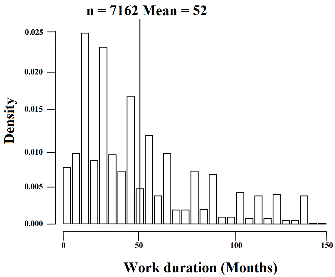
One way to consider the impact of such early life cycle predictors is to use the data of Figure 2. That plot shows that software employees usually change projects every 52 months (either moving between companies or changing projects within an organization). This means that in seven years (84 months), the majority of workers and managers would first appear on a job after the initial four months required to learn a defect predictor. Hence, for most workers and managers, the detectors learned via the methods of this paper would be the “established wisdom” and “the way we do things here” for their projects. This means that a detector learned in the first four months would be a suitable oracle to guide training and hiring; the development of code review practices; the automation of local “bad smell detectors”; as well as tool selection and development.

Paper	Year	Citations	Sampling	Projects	Paper	Year	Citations	Sampling	Projects	Paper	Year	Citations	Sampling	Projects
[31]	2008	172	All	12	[20]	2016	111	Release	17	[32]	2018	61	All	9
[33]	2010	21	All	5	[34]	2016	28	Release	10	[35]	2018	43	Percentage	101
[36]	2010	347	Percentage	10	[37]	2016	130	Release	10	[38]	2018	15	Release	13
[39]	2011	94	All	8	[40]	2017	44	All	6	[41]	2019	16	Percentage	7
[2]	2012	264	All	11	[16]	2017	36	Month	6	[42]	2019	14	Month	10
[1]	2012	387	All	5	[43]	2017	220	All	34	[44]	2019	11	Percentage	26
[45]	2013	322	All	10	[46]	2017	44	Percentage	255	[47]	2019	14	Slice	6
[48]	2014	105	All	1,403	[49]	2017	8	All	10	[50]	2019	1	All	10
[51]	2014	44	Release	1	[52]	2018	36	All	11	[53]	2019	0	Percentage	6
[13]	2014	93	Release	5	[54]	2018	66	Percentage		[55]	2019	4	Release	9
[18]	2015	129	All	7	[56]	2018	33	All	18	[57]	2019	10	Release	20
[58]	2016	87	All	10	[59]	2018	25	All	16	[17]	2019	8	All, Slice	2
[60]	2016	42	Release	23	[61]	2018	40	All	6	[19]	2020	0	All	6

TABLE I: Papers discussing different sampling policies. All (papers that utilize all historical data to build defect prediction models, shaded in gray).

III Why Early Defect Prediction Might Work

III-A GitHub Results

Recently (2020), Shrikanth and Menzies found defect-prediction beliefs not supported by available evidence [29]. We looked for why such confusions exist – which lead to the discovery that pattern in Figure 1 of project data changes dramatically over the life-cycle. Figure 1 shows data from 1.2m GitHub commits from 155 popular GitHub projects (the criteria for selecting those particular projects is detailed below). Note how the frequency defect data (shown in red/shaded) starts collapsing early in the life cycle (after 12 months). This observation suggests that it might be relatively uninformative to learn from later life cycle data. This was an interesting finding since, as mentioned in the introduction, it is common practice in defect prediction to perform “recent validation” where predictors are tested on the latest release after training from the prior one or two releases [18, 16, 19]. In terms of Figure 1, that strategy would train on red dots (shaded) taken near the right-hand-side, then test on the most right-hand-side dot. Given the shallowness of the defect data in that region, such recent validation could lead to results that are not representative of the whole life cycle.

Accordingly, we sat out to determine how different training and testing sampling policies across the life cycle of Figure 1 affected the results. After much experimentation (described below), we assert that if data is collected up until the vertical green line of Figure 1, then that generates a model as good as anything else.

III-B Related Work

Before moving on, we first discuss related work on early life cycle defect prediction. In 2008, Fenton et al. [62] explored the use of human judgment (rather than data collected from the domain) to handcraft a causal model to predict residual defects (defects caught during independent testing or operational usage) [62]. Fenton needed two years of expert interaction to build models that compete with defect predictors learned by data miners from domain data. Hence we do not explore those methods here since they were very labor-intensive.

In 2010, Zhang and Wu showed that it is possible to estimate the project quality with fewer programs sampled from an entire space of programs (covering the entire project life-cycle) [63]. Although we too draw fewer samples (commits), we sample them ‘early’ in the project life-cycle to build defect prediction models. In another 2013 study about sample size, Rahman et al. stress the importance of using a large sample size to overcome bias in defect prediction models [14]. We find our proposed ‘data-lite’ approach performs similar to ‘data-hungry’ approaches while we do not deny bias in defect prediction data sets. Our proposed approach and recent defect prediction work handle bias by balancing defective and non-defective samples [57, 32] (class-imbalance).

Recently (2020), Arokiam and Jeremy [64] explored bug severity prediction. They show it is possible to predict bug-severity early in the project development by using data transferred from other projects [64]. Their analysis was on the cross-projects, but unlike this paper, they did not explore just how early in the life cycle did within project data became effective. In similar work to Arokiam and Jeremy, in 2020, Sousuke  [15] explored another early life cycle, Cross-Version defect prediction (CVDP) using Cross-Project Defect Prediction (CPDP) data. Their study was not as extensive as ours (only 41 releases). CVDP uses the project’s prior releases to build defect prediction models. Sousuke compared defect prediction models trained using three within project scenarios (recent project release, all past releases, and earliest project release) to endorse recent project release. Sousuke also combined CVDP scenarios using CPDP (24 approaches) to recommend that the recent project release was still better than most CPDP approaches. However, unlike Sousuke, we offer contrary evidence in this work, as our endorsed policy based on earlier commits works similar to all other prevalent policies (including the most recent release) reported in the literature. Notably, we assess our approach on 1000+ releases and evaluate on seven performance measures.

In summary, as far as we can tell, ours is the first study to perform an extensive comparison of prevalent sampling policies practiced in the defect prediction space.

IV Sampling Polices

One way to summarize this paper is to evaluate a novel “stop early” sampling policy for collecting the data needed for defect prediction. This section describes a survey of sampling policies in defect prediction. Each sampling policy has its way of extracting training and test data from a project. As shown below, there is a remarkably diverse number of policies in the literature that have not been systematically and comparatively evaluated prior to this paper.

In April 2020, we found 737 articles in Google Scholar using the query (“software” AND “defect prediction” AND “just in time”, “software” AND “ defect prediction” AND “sampling policy”). “Just in time (JIT)” defect prediction is a widely-used approach where the code seen in each commit is assessed for its defect proneness [2, 65, 19, 18].

From the results of that query, we applied some temporal filtering: (1) we examined all articles more recent than 2017; (ii) for older articles, we examined all papers from the last 15 years with more than 10 citations per year. After reading the title, abstracts, and the methodology sections, we found the 39 articles of Table I that argued for particular sampling policies.

Figure 3: Summary of sampling types from Table I.

Figure 3 shows a high-level view of the sampling policies seen in the Table I papers:

• All: When the historical data (commits/files/modules etc) is used for evaluation within some cross-validation study (where the data is divided randomly into $N$ bins and the data from bin ‘$i\in N$’ is used to test a model trained from all other data) [1].

• Percentage: The historical data is stratified by some percentage, like 80-20%. The minimum % we found was 67% [35].

• Release: The models are trained on the immediate or more past releases in order to predict defects on the current release [57].

• Month: When 3 or 6 months of historical data is used to predict defects in future files, commits, or release [16].

• Slice: An arbitrary stratification is used to divide the data based on a specific number of days (like 180 days or six months in [48]).

Figure 4: A visual map of sampling. Project time-line divided into ‘Train commits’ and ‘Test commits’. Learners learn from ‘Train’ to classify defective commits in the ‘Test’.

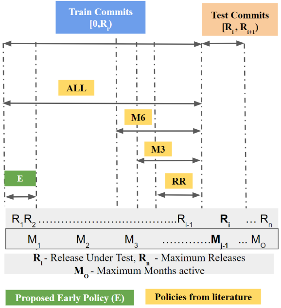
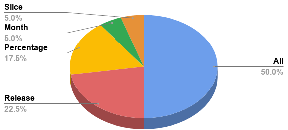
It turns out Figure 3 is only an approximation of the diverse number sampling policies we see in the literature. A more comprehensive picture is shown in Figure 4 where we divide software releases $R_{i}$ that occur over many months $M_{j}$ into some train and test set.

TABLE II: Four representative sampling policies from literature and an early life cycle policies (the row shown in gray).

Policy	Method
ALL	Train using all past software commits ($[0,R_{i})$) in the project before the first commit in the release under test $R_{i}$.
M6	Train using the recent six months of software commits ($[R_{i}-6months)$) made before the first commit in the release under test $R_{i}$.
M3	Train using the recent three months of software commits ($[R_{i}-3months)$) made before the first commit in the release under test $R_{i}$.
RR	Train using the software commits in the previous release $R_{i-1}$ before the first commit in the release under test $R_{i}$.
E	Train using early 50 commits (25 clean and 25 defective) randomly sampled within the first 150 commits before the first commit in the release under test $R_{i}$.

Using a little engineering judgment and guided by the frequency of different policies (from Figure 3), we elected to focus on four sampling policies from the literature and one ‘early stopping’ policy, see Table II). The % share in Figure 3 show ‘ALL and RR’ are prevalent practices whereas ‘M3 and M6’ though not prevalent are used in related literature [16, 17]. We did not consider separate policies for ‘Percentage’ and ‘Slice’ as the former is similar to ‘ALL’ (100% of historical data), and the latter is least prevalent and similar to M6 (180 days or six months).

Note the “magic numbers” in Table II:

• 3 months, 6 months: these are thresholds often seen in the literature.

• 25 clean + 25 defective commits: We arrived at these numbers based on the work of Nam et al. built defect prediction models for using just 50 samples [43].

• Sampling at random from the first 150 commits. Here, we did some experiments recursively dividing the data in half until defect prediction stopped working.

We will show below that early sampling (shown in gray in Table II) works just as well as the other policies.

V Methods

V-A Data

This section describes the data used in this study as well as what we mean by “clean” and “defective” commits.

All our data comes from open source (OS) GitHub projects [7] that we mined randomly using Commit Guru [66]. Commit Guru is a publicly available tool based on a 2015 ESEC/FSE paper used in numerous prior works [67, 19]. Commit Guru provides a portal where it takes a request (URL) to process a GitHub repository. It extracts all commits and their features to be exported to a file. Commits are categorized (based on the occurrence of certain keywords) similar to the approach in SZZ algorithm [68]. The “defective” (bug-inducing) commits are traced using the git diff (show changes between commits) feature from bug fixing commits; the rest are labeled “clean”.

But data from Commit Guru does not contain release information, which we extract separately from the project tags. Then we use scripts to associate the commits to the release dates. Then those codes associated with those changes were then summarized by Commit Guru using the attributes of Table III. Those attributes became the independent attributes used in our analysis. Note that the use of these particular attributes has been endorsed by prior studies  [2, 69].

SE researchers have warned against using all GitHub data since this website contains many projects that might be categories as “non-serious” (such as homework assignments). Accordingly, following the advice of prior researchers [5, 4], we ignored projects with

• Less than 1000 stars;

• Less than 1% defects;

• Less than two releases;

• Less than one year of activity;

• No license information.

• Less than 5 defective and 5 clean commits.

This resulted in 155 projects developed written in many languages across various domains, as discussed in §I.

TABLE III: 14 Commit level features that Commit Guru tool [2, 66] mines from GitHub repositories

Dimension	Feature	Definition
	NS	Number of modified subsystems
	ND	Number of modified directories
	NF	Number of modified Files
Diffusion	ENTROPY	Distribution of modified code across each file
	LA	Lines of code added
	LD	Lines of code deleted
Size	LT	Lines of code in a file before the change
Purpose	FIX	Whether the change is defect Changes that fixing the defect are more likely to introduce more defects fixing ?
	NDEV	Number of developers that changed the modified files
	AGE	The average time interval from the last to the current change
History	NUC	Number of unique changes to the modified files before
	EXP	Developer experience
	REXP	Recent developer experience
Experience	SEXP	Developer experience on a subsystem

Figure 5: Distributions seen in all 1.2 millions commits of all 155 projects: median values of commits (3,728), percent of defective commits (20%), life span in years (7), releases (59) and stars (9,149).

Figure 6: Distributions seen in the first 150 commits of all 155 projects; median values of project releases (5), project development months (4) and defective commits (41)

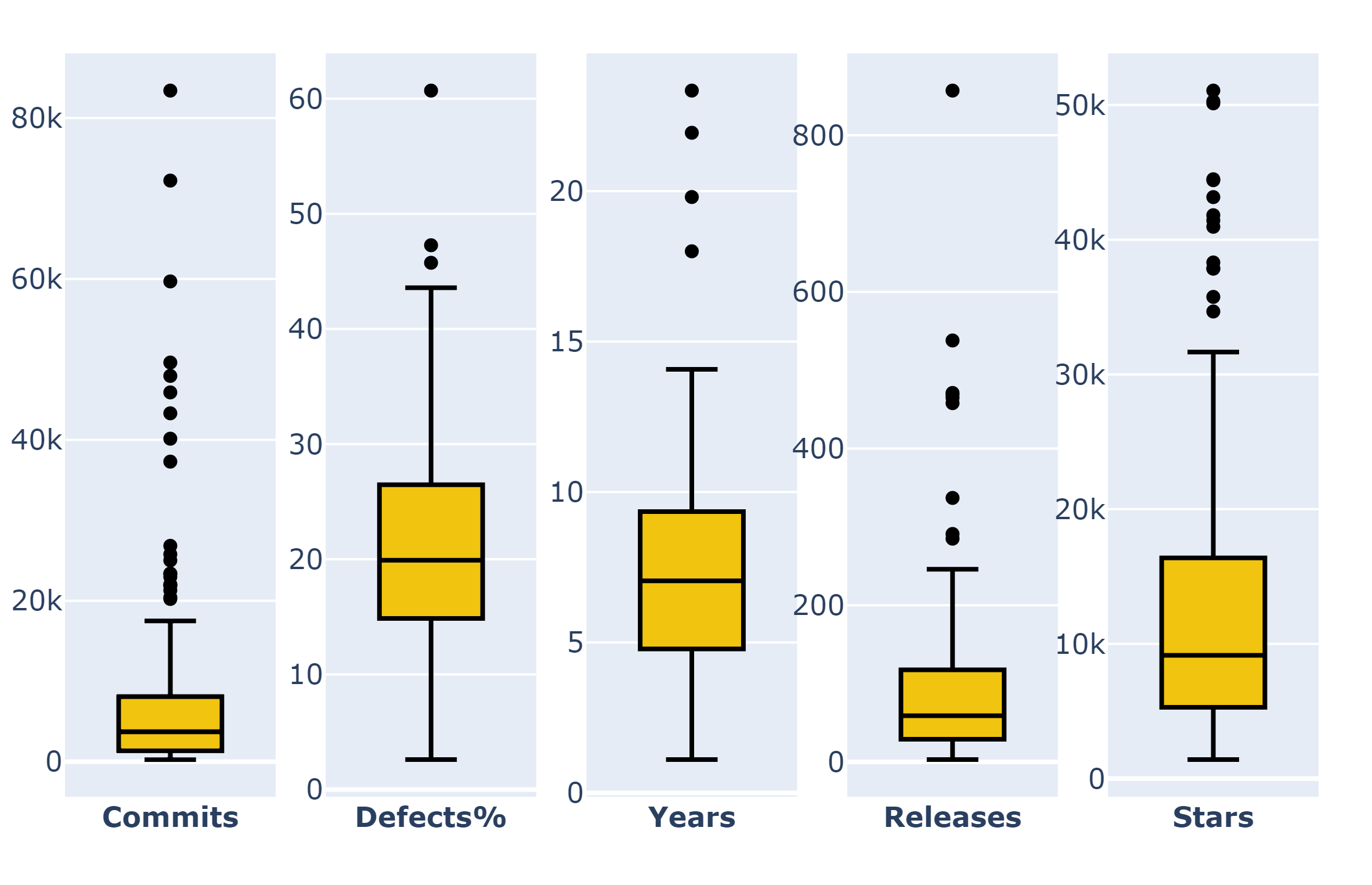
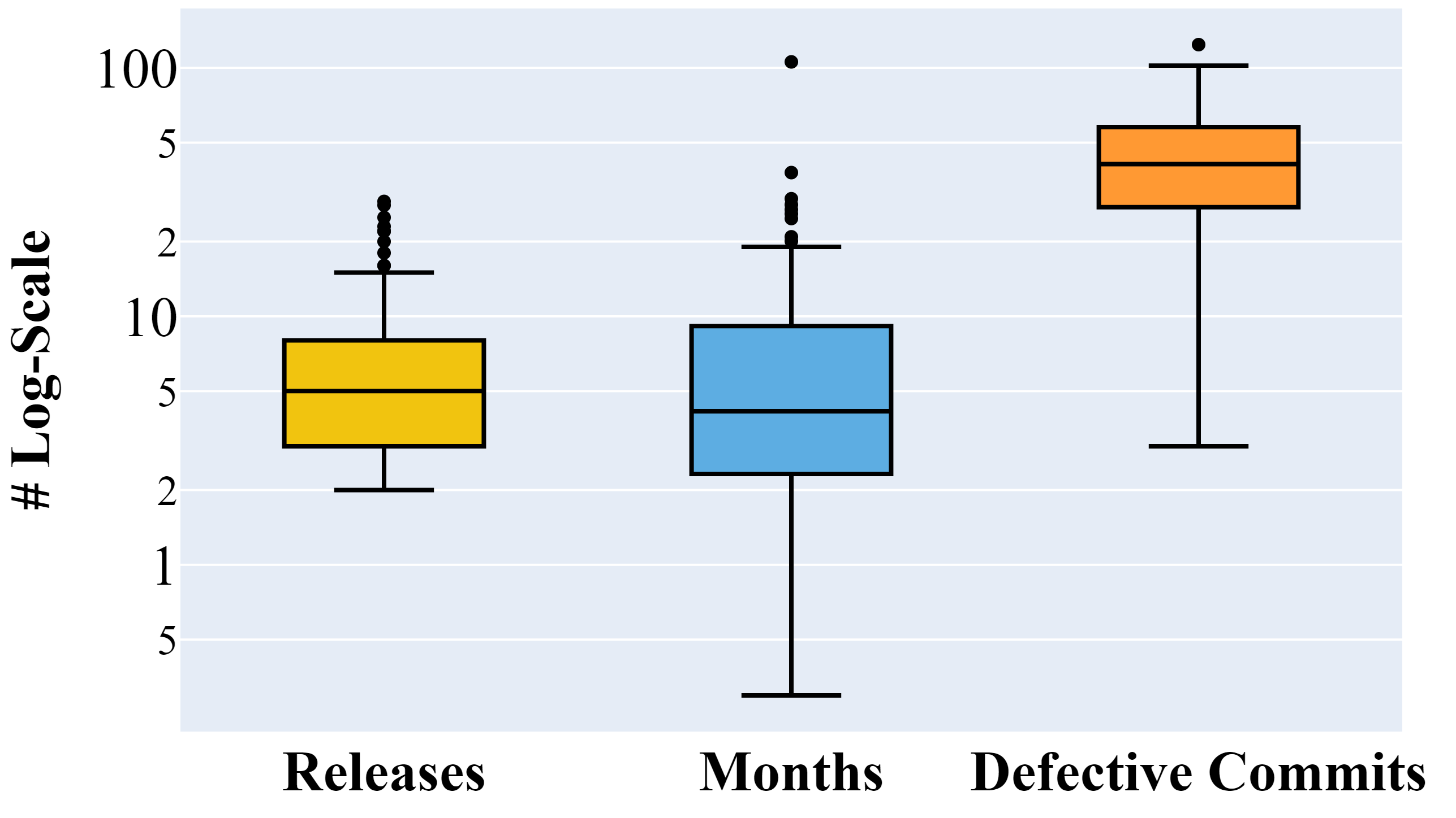
Figure 5 shows information on our selected projects. As shown in that figure, our projects have:

• Median life spans of 84 months with 59 releases;

• The projects have (265, 3,728, 83,409) commits (min, median, max) with data up to December 2019;

• 20% (median) of project commits introduce bugs.

Figure 6 focuses on just the data used in the early life cycle ” E ” sampler described in Figure 4. In the median case, by the time we can collect 150 commits, projects have had five releases in 4 months (median values).

V-B Algorithms

Our study uses three sets of algorithms:

• The five sampling policies described above;

• The six classifiers described here;

• Pre-processing for some of the sampling policies.

V-B1 Classifiers

After an extensive analysis, Ghotra et al.  [70] rank over 30 defect prediction algorithms into four ranks. For our work, we take six of their learners that are widely used in the literature and which can be found at all four ranks of the Ghtora et al., study. Those learners were:

• Logistic Regression (LR);

• Nearest neighbour (KNN) (minimum 5 neighbors);

• Decision Tree (DT);

• Random Forrest (RF)

• Naïve Bayes (NB);

• Support Vector Machines (SVM)

V-B2 Pre-processers

Following some advice from the literature, we applied some feature engineering to the Table III data. Based on advice by Nagappan and Ball, we generated relative churn and normalized LA and LD attributes by dividing by LT and LT and NUC dividing by NF [71]. Also, we dropped ND and REXP since Kamei et al. reported that NF and ND are highly correlated with REXP and EXP. Lastly, we applied the logarithmic transform to the remaining process measures (except the boolean variable ‘FIX’) to alleviate skewness [72].

In other pre-processing steps, we applied Correlation-based Feature Selection (CFS). Our initial experiments with this data set lead to unpromising results (recalls less than 40%, high false alarms). However, those results improved after we applied feature subset selection to remove spurious attributes. CFS is a widely applied feature subset selection method proposed by Hall  [73] and is recommended in building supervised defect prediction models [44]. CFS is a heuristic-based method to find (evaluate) a subset of features incrementally. CFS performs a best-first search to find influential sets of features that are not correlated with each other, however, correlated with the classification. Each subset is computed as follows: $\mathit{merit}s=kr{\mathit{cf}}/\sqrt{k+k(k-1)r_{\mathit{ff}}}$ where:

• $\mathit{merit}s$ is the value of subset $s$ with $k$ features;

• $r{\mathit{cf}}$ is a score that explains the connection of that feature set to the class;

• $r{\mathit{ff}}$ is the feature to feature mean and connection between the items in $s$, where $r{\mathit{cf}}$ should be large and $r_{\mathit{ff}}$.

Another pre-processor that was applied to some sampling policies was Synthetic Minority Over-Sampling, or SMOTE. When the proportion of defective and clean commits (or modules, files, etc.) is not equal, learners can struggle to find the target class. SMOTE, proposed by Chawla et al.  [74] is often applied in defect prediction literature to overcome this problem [32, 54]. To achieve balance, SMOTE artificially synthesizes examples (commits) extrapolating using K-nearest neighbors (minimum five commits required) in the data set (training commits in our case) [74]. Note that:

• We do not apply SMOTE to policies that already guarantee class balancing. For example, our preferred early life-cycle method selects at random 25 defective, and 25 non-defective (clean) commits from the first 150 commits.

• Also, just to document that we avoided a potential methodological error [32], we record here that we applied SMOTE to the training data, but never the test data.

V-C Evaluation Criteria

Defect prediction studies evaluated their model performance using a variety of criteria. From the literature, we used what we judged to be the most widely-used measures [31, 45, 54, 57, 48, 16, 35, 19, 55, 50, 46, 1, 2]. For the following seven criteria:

• Nearly all have the range 0 to 1 (except Initial number of False Alarms, which can be any positive number);

• Four of these criteria need to be minimized: D2H, IFA, Brier, PF; i.e., for these criteria less is better.

• Three of these criteria need to be maximized: AUC, Recall, G-Measure; i.e. for these criteria more is better.

One reason we avoid precision is that prior work shows this measure has significant issues for unbalanced data [31].

V-C1 Brier

Recent defect prediction papers [16, 54, 35, 19] measure the model performance using the Brier absolute predictive accuracy measure. Let $C$ be the total number of the test commits. Let $y_{i}$ be 1 (for defective commits) or 0 otherwise. Let $\hat{y_{i}}$ be the probability of commit being defective (calculated from the loss functions in scikit-learn classifiers [75]). Then:

$$\footnotesize\mathit{Brier}=\frac{1}{C}\sum\limits_{t=1}^{C}(y_{i}-\hat{y_{i}})^{2}\,\!\$$ (1)

V-C2 Initial number of False Alarms (IFA)

Parnin and Orso  [76] say that developers lose faith in analytics if they see too many initial false alarms. IFA is simply the number of false alarms encountered after sorting the commits in the order of probability of being detective, then counting the number of false alarms before finding the first true alarm.

V-C3 Recall

Recall is the proportion of inspected defective commits among all the actual defective commits.

$$\footnotesize\mathit{Recall}=\frac{\mathit{True\ Positives}}{\mathit{True\ Positives+False\ Negatives}}$$ (2)

V-C4 False Positive Rate (PF)

The proportion of predicted defective commits those are not defective among all the predicted defective commits.

$$\footnotesize\mathit{PF}=\frac{\mathit{False\ Positives}}{\mathit{False\ Positives+True\ Negatives}}$$ (3)

V-C5 Area Under the Receiver Operating Characteristic curve (AUC)

AUC is the area under the curve between the true positive rate and false-positive rate.

V-C6 Distance to Heaven (D2H)

D2H or “distance to heaven” aggregates on two metrics Recall and False Positive Rate (PF) to show how close to “heaven” (Recall=1 and PF=0) [77].

$$\footnotesize\mathit{D2H}=\frac{\sqrt{(1-\mathit{Recall})^{2}+(0-\mathit{PF})^{2}}}{\sqrt{2}}$$ (4)

V-C7 G-measure (GM)

A harmonic mean between Recall and the compliment of PF measured, as shown below.

$$\footnotesize\mathit{G-Measure}=\frac{2*\mathit{Recall}*(1-\mathit{PF})}{\mathit{Recall}+(1-\mathit{PF})}$$ (5)

Even though GM and D2H combined the same underlying measures, we include both here since they both have been used separately in the literature. Also, as shown below, it is not necessarily true that achieving good results on GM means that good results will also be achieved with D2H.

Due to the nature of the classification process, some criteria will always offer contradictory results:

• A learner can achieve 100% recall just by declaring that all examples belong to the target class. This method will incur a high false alarm rate.

• A learner can achieve 0% false alarms just by declaring that no examples belong to the target class. This method will incur a very low recall rate.

• Similarly, Brier and Recall are also antithetical since reducing the loss function also means missing some conclusions and lowering recall.

V-D Statistical Test

Later in §VI, we compare distributions of evaluation measures of various sampling policies that may have the same median while their distribution could be very different. Hence to identify significant differences (rank) among two or more populations, we use the Scott-Knott test recommended by Mittas et al. in TSE’13 paper [78]. This test is a top-down bi-clustering approach for ranking different treatments, sampling policies in our case. This method sorts a list of $l$ sampling policy evaluations with $\mathit{ls}$ measurements by their median score. It then splits $l$ into sub-lists m, n in order to maximize the expected value of differences in the observed performances before and after divisions.

For lists $l,m,n$ of size $\mathit{ls},\mathit{ms},\mathit{ns}$ where $l=m\cup n$, the “best” division maximizes $E(\Delta)$; i.e. the difference in the expected mean value before and after the spit:

$$E(\Delta)=\frac{ms}{ls}abs(m.\mu-l.\mu)^{2}+\frac{ns}{ls}abs(n.\mu-l.\mu)^{2}$$

We also employ the conjunction of bootstrapping and A12 effect size test by Vargha and Delaney [79] to avoid “small effects” with statistically significant results.

Important note: we apply our statistical methods separately to all the evaluation criteria; i.e., when we compute ranks, we do so for (say) false alarms separately to recall.

V-E Experimental Rig

By definition, our different sampling policies have different train and different test sets. But, methodologically, when we compare these different policies, we have to compare results on the same sets of releases. To handle this we:

• First, run all our six policies, combined with all our six learners. This offers multiple predictions to different commits.

• Next, for each release, we divide the predictions into those that come from the same learner:policy pair. These divisions are then assessed with statistical methods described above.

Policy	Classifier	Wins	D2H-	AUC+	IFA-	Brier-	Recall+	PF-	GM+
M6	NB	4	0.37	0.67	1.0	0.32	0.78	0.33	0.67
M3	NB		0.37	0.67	1.0	0.31	0.76	0.32	0.68
E	LR		0.36	0.68	1.0	0.32	0.71	0.31	0.68
M6	SVM		0.43	0.65	0.0	0.21	0.44	0.1	0.48
M3	SVM		0.43	0.65	0.0	0.21	0.43	0.1	0.48
ALL	NB	3	0.4	0.65	1.0	0.36	0.83	0.40	0.67
E	KNN	2	0.39	0.65	1.0	0.33	0.65	0.32	0.62
ALL	LR		0.38	0.66	1.0	0.3	0.65	0.25	0.62
M6	LR		0.36	0.68	1.0	0.25	0.59	0.19	0.60
M3	LR		0.36	0.68	1.0	0.24	0.58	0.17	0.60
M6	KNN		0.4	0.65	0.0	0.23	0.50	0.14	0.53
ALL	SVM		0.4	0.66	0.0	0.25	0.50	0.14	0.54
M3	KNN		0.41	0.65	0.0	0.23	0.47	0.13	0.51
M6	RF		0.44	0.63	0.0	0.24	0.43	0.12	0.47
E	SVM	1	0.4	0.64	1.0	0.31	0.6	0.26	0.59
ALL	KNN		0.38	0.66	1.0	0.25	0.55	0.17	0.57
ALL	DT		0.42	0.62	1.0	0.32	0.52	0.25	0.54
M6	DT		0.43	0.62	1.0	0.29	0.5	0.2	0.51
ALL	RF		0.42	0.64	1.0	0.26	0.49	0.15	0.51
M3	DT		0.43	0.62	1.0	0.28	0.48	0.19	0.5
M3	RF		0.44	0.63	1.0	0.24	0.42	0.11	0.46
E	DT	0	0.46	0.58	1.0	0.38	0.57	0.35	0.54
E	NB		0.54	0.54	1.0	0.37	0.55	0.29	0.41
E	RF		0.44	0.61	1.0	0.33	0.52	0.26	0.52

KEY:   More data (ALL,M6 and M3) Early (E)

TABLE IV: 24 defect prediction models tested in all 4,876 applicable project releases. In the first row “+” and “-” denote the criteria that need to be maximized or minimized, respectively. ‘Wins’ is the frequency of the policy found in the top #1 Scott-Knott rank in each of the seven evaluation measures (the cells shaded in gray).

Policy	Classifier	Wins	D2H-	AUC+	IFA-	Brier-	Recall+	PF-	GM+
E	LR	4	0.36	0.68	1.0	0.32	0.71	0.31	0.68
RR	NB	3	0.38	0.66	1.0	0.32	0.71	0.30	0.65
RR	LR	3	0.35	0.68	1.0	0.24	0.59	0.18	0.61
RR	SVM	3	0.42	0.64	0.0	0.23	0.47	0.12	0.5
E	KNN	2	0.39	0.64	1.0	0.34	0.64	0.32	0.62
RR	KNN	2	0.41	0.64	1.0	0.25	0.5	0.15	0.53
RR	RF	2	0.43	0.63	1.0	0.24	0.43	0.13	0.48
E	SVM	1	0.4	0.64	1.0	0.31	0.6	0.26	0.59
E	DT	0	0.46	0.58	1.0	0.39	0.56	0.35	0.54
E	NB	0	0.54	0.54	1.0	0.37	0.54	0.29	0.42
E	RF	0	0.44	0.61	1.0	0.33	0.52	0.26	0.53
RR	DT	0	0.42	0.62	1.0	0.28	0.50	0.20	0.51

KEY: Recency (RR) Early (E)

TABLE V: 12 defect prediction models tested on 3,704 project releases. In the first row “+” and “-” denote criteria that need to be maximized or minimized, respectively. ‘Wins’ is the frequency of the policy found in the top #1 Scott-Knott rank in each of the seven evaluation measures (the cells shaded in gray).

VI Results

Tables IV and V show results when our six learners applied our five sampling policies. We splot these results into two tables since Our policies lead to results with different samples sizes: the recent release, or “RR”, the policy uses data from just two releases while “ALL” uses everything.

In the first row of those tables, “+” and “-” denote criteria that need to be maximized or minimized, respectively. Within the tables, gray cells show statistical test results (conducted separately on each criterion). Anything ranked “best” is colored gray, while all else have white backgrounds.

Columns one and two show the policy/learners that lead to these results. Rows are sorted by how often policy/learners “win”; i.e., achieve best ranks across all criteria. In Tables IV and V, no policy+learner wins 7 out of 7 times on all criteria, so some judgment will be required to make an overall conclusion. Specifically, based on results from the multi-objective optimization literature, we will first remove the policies+learners that score worse on most criteria, then debate trade-offs between the rest.

To simplify that trade-off debate, we offer two notes. Firstly, cross all our learners, the median value for IFA is very small– zero or one; i.e., developers using these tools only need to suffer one false alarm or less before finding something they need to fix. Since these observed IFA scores are so small, we say that “losing” on IFA is hardly a reason to dismiss a learner/sampler combination. Secondly, D2H and GM combine multiple criteria. For example, “winning” on D2H and GM means performing well on both Recall and PF; i.e. these two criteria are somewhat more informative than the others.

Turning now to those results, we explore two issues. For defect prediction:

RQ1: Is more data, better?

RQ2: When is more recent data better than older data?

Note that we do explore a third research issue: are different learners better at learning from a little, a lot, or all the available data. Based on our results, we have nothing definitive to offer on that issue. That said, if we were pressed to recommend a particular learning algorithm, then we say there are no counterexamples to the claim that “it is useful to apply CFS+LR”.

RQ1: Is more data, better?

Belief1: Our introduction included examples where proponents of data-hungry methods advocated that if data is useful, then even more data is much more useful.

Prediction:1 If that belief was the case, then in Table IV, data-hungry sampling policies that used more data should defeat “data-lite” sampling policies.

Observation1a: In Table IV, Our “data hungriest” sampling policy (ALL) loses on on most criteria. While it achieves the highest Recall (83%), it also has the highest false alarm range (40%). As to which other policy is preferred in the best wins=4 zone of Table IV, there is no clear winner. What we would say here is that our preferred “data-lite” method called “E” (that uses 25 defective and 25 non-defective commits selected at random from the first 150 commits) is competitive with the rest. Hence:

Observations1b: Figure 5 of this paper showed that within our sample of projects, we have data lasting a median of 84 months. Figure 6 noted that by the time we get to 150 commits, most projects are 4 months old (median values). The “E” results of Table IV showed that defect models learned from that 4 months of data are competitive with all the other policies studied here. Hence we say,

RQ2: When is more recent data better than older data?

Belief2: As discussed earlier in our introduction, many researchers prefer using recent data over data from earlier periods. For example, it is common practice in defect prediction to perform “recent validation” where predictors are tested on the latest release after training from the prior one or two releases [18, 16, 19, 20]. For a project with multiple releases, recent validation ignores all the insights that are available from older releases.

Prediction2: If recent data is comparatively more informative than older data, then defect predictors built on recent data should out-perform predictors built on much older data.

Observations2: We observe that:

• Figure 5 of this paper showed that within our sample of projects, we have data lasting a median of 84 months.

• Figure 6 noted that by the time we get to 150 commits, most projects are 4 months old (median values).

• Table V says that “E” wins over “RR” since it falls in the best wins=4 section.

• Hence we could conclude that older data is more effective than recent data.

That said, we feel somewhat more the circumspect conclusion is in order. When we compare E+LR to the next learner in that table (RR+NB) we only find a minimal difference in their performance scores. Hence we make a somewhat humbler conclusion:

This is a startling result for two reasons. Firstly, compared to the “RR” training data, the “E” training data is very old indeed. For projects lasting 84 months long, “RR” is trained on information from recent few months, with “E” data comes from years before that. Secondly, this result calls into question any conclusion made in a paper that used recent validation to assess their approach; e.g. [18, 16, 19, 20].

VII Threats to Validity

VII-A Sampling Bias

The conclusion’s generalizability will depend upon the samples considered; i.e., what matters here may not be true everywhere. To improve our conclusion’s generalizability, we mined 155 long-running OS projects that are developed for disparate domains and written in numerous programming languages. Sampling trivial projects (like homework assignments) is a potential threat to our analysis. To mitigate that, we adhered to the advice from prior researchers as discussed earlier in §I and §V-A. We find our sample of projects have 20% (median) defects as shown in Figure 5 nearly the same as data used by Tantithamthavorn et al. [35] who report 30% (median) defects.

VII-B Learner bias

Any single study can only explore a handful of classification algorithms. For building the defect predictors in this work, we elected six learners (Logistic Regression, Nearest neighbor, Decision Tree, Support Vector Machines, Random Forrest, and Naïve Bayes). These six learners represent a plethora of classification algorithms [70].

VII-C Evaluation bias

We use seven evaluation measures (Recall, PF, IFA, Brier, GM, D2H, and AUC). Other prevalent measures in this defect prediction space include precision. However, as mentioned earlier, precision has issues with unbalanced data [31].

VII-D Input Bias

Our proposed sampling policy ‘E’ randomly samples 50 commits from early 150 commits. Thus it may be true that different executions could yield different results. However, this is not a threat because each time, the early policy ‘E ’ randomly samples 50 commits from early 150 commits to test sizeable 8,490 releases (from Table IV and Table V) across all the six learners. In other words, our conclusions about ‘E’ hold on a large sample size of numerous releases.

VIII Conclusion

When data keep changing, the models we can learn from that data may also change. If conclusions become too fluid (i.e., change too often), then no one has a stable basis for making decisions or communicating insights.

Issues with conclusion instability disappear if, early in the life cycle, we can learn a predictive model that is effective for the rest of the project. This paper has proposed a methodology for assessing such early life cycle predictors.

1. Define a project selection criteria. For this paper, our selection criteria are taken from related work (from recent EMSE, TSE papers [5, 4]);

2. Select some software analytics task. For this paper, we have explored learning defect predictors.

3. See how early projects selected by the criteria can be modeled for that task. Here we found that defect predictors learned from the first four months of data perform as well as anything else.

4. Conclude that projects matching criteria need more data for task before time found in step 3. In this paper, we found that for 96% of the time, we neither want nor need data-hungry defect prediction.

We stress that this result has only been shown here for defect prediction and only for the data selected by our criteria.

As for future work, we have many suggestions:

• The clear next step in this work is to check the validity of this conclusion beyond the specific criteria and task explored here.

• We need to revisit all prior results that used recent validation to assess their approach; e.g. [18, 16, 19, 20] since our RQ2 suggests they may have been working in a relatively uninformative region of the data.

• While the performance scores of Tables IV and V are reasonable, there is still much room for improvement. Perhaps if we augmented early life cycle defect predictors with a little transfer learning (from other projects [43]), then we could generate better performing predictors.

• Further to the last point, another interesting avenue of future research might be hyper-parameter optimization (HPO) [80, 20, 81]. HPO is often not applied in software analytics due to its computational complexity. Perhaps that complexity can be avoided by focusing only on small samples of data from very early in the life cycle.

References

- [1] M. D’Ambros, M. Lanza, and R. Robbes, “Evaluating defect prediction approaches: a benchmark and an extensive comparison,” Empirical Software Engineering, vol. 17, no. 4-5, pp. 531–577, 2012.
- [2] Y. Kamei, E. Shihab, B. Adams, A. E. Hassan, A. Mockus, A. Sinha, and N. Ubayashi, “A large-scale empirical study of just-in-time quality assurance,” IEEE Transactions on Software Engineering, vol. 39, no. 6, pp. 757–773, 2012.
- [3] P. Norvig. (2011) The Unreasonable Effectiveness of Data. Youtube. [Online]. Available: https://www.youtube.com/watch?v=yvDCzhbjYWs
- [4] N. Munaiah, S. Kroh, C. Cabrey, and M. Nagappan, “Curating github for engineered software projects,” Empirical Software Engineering, vol. 22, no. 6, pp. 3219–3253, 2017.
- [5] M. Yan, X. Xia, Y. Fan, A. E. Hassan, D. Lo, and S. Li, “Just-in-time defect identification and localization: A two-phase framework,” IEEE Transactions on Software Engineering, 2020.
- [6] R. Abdalkareem, V. Oda, S. Mujahid, and E. Shihab, “On the impact of using trivial packages: an empirical case study on npm and pypi,” Empirical Software Engineering, vol. 25, no. 2, pp. 1168–1204, Mar. 2020. [Online]. Available: https://doi.org/10.1007/s10664-019-09792-9
- [7] “GitHub Inc - provides hosting for software development version control using git.” https://github.com/, accessed: 2019-03-18.
- [8] T. J. Ostrand, E. J. Weyuker, and R. M. Bell, “Predicting the location and number of faults in large software systems,” IEEE Transactions on Software Engineering, vol. 31, no. 4, pp. 340–355, 2005.
- [9] T. Menzies, J. Greenwald, and A. Frank, “Data mining static code attributes to learn defect predictors,” IEEE transactions on software engineering, vol. 33, no. 1, pp. 2–13, 2006.
- [10] Z. Wan, X. Xia, A. E. Hassan, D. Lo, J. Yin, and X. Yang, “Perceptions, expectations, and challenges in defect prediction,” IEEE Transactions on Software Engineering, 2018.
- [11] A. T. Misirli, A. Bener, and R. Kale, “Ai-based software defect predictors: Applications and benefits in a case study,” AI Magazine, vol. 32, no. 2, pp. 57–68, 2011.
- [12] M. Kim, D. Cai, and S. Kim, “An empirical investigation into the role of api-level refactorings during software evolution,” in Proceedings of the 33rd International Conference on Software Engineering. ACM, 2011, pp. 151–160.
- [13] F. Rahman, S. Khatri, E. T. Barr, and P. Devanbu, “Comparing static bug finders and statistical prediction,” in Proceedings of the 36th International Conference on Software Engineering, ser. ICSE 2014. New York, NY, USA: Association for Computing Machinery, 2014, p. 424–434. [Online]. Available: https://doi.org/10.1145/2568225.2568269
- [14] F. Rahman, D. Posnett, I. Herraiz, and P. Devanbu, “Sample size vs. bias in defect prediction,” in Proceedings of the 2013 9th joint meeting on foundations of software engineering. ACM, 2013, pp. 147–157.
- [15] S. Amasaki, “Cross-version defect prediction: use historical data, cross-project data, or both?” Empirical Software Engineering, pp. 1–23, 2020.
- [16] S. McIntosh and Y. Kamei, “Are fix-inducing changes a moving target? a longitudinal case study of just-in-time defect prediction,” IEEE Transactions on Software Engineering, vol. 44, no. 5, pp. 412–428, 2017.
- [17] T. Hoang, H. Khanh Dam, Y. Kamei, D. Lo, and N. Ubayashi, “Deepjit: An end-to-end deep learning framework for just-in-time defect prediction,” in 2019 IEEE/ACM 16th International Conference on Mining Software Repositories (MSR), 2019, pp. 34–45.
- [18] M. Tan, L. Tan, S. Dara, and C. Mayeux, “Online defect prediction for imbalanced data,” in 2015 IEEE/ACM 37th IEEE International Conference on Software Engineering, vol. 2. IEEE, 2015, pp. 99–108.
- [19] M. Kondo, D. M. German, O. Mizuno, and E.-H. Choi, “The impact of context metrics on just-in-time defect prediction,” Empirical Software Engineering, vol. 25, no. 1, pp. 890–939, 2020.
- [20] W. Fu, T. Menzies, and X. Shen, “Tuning for software analytics: Is it really necessary?” Information and Software Technology, vol. 76, pp. 135–146, 2016.
- [21] T. Zimmermann, N. Nagappan, H. Gall, E. Giger, and B. Murphy, “Cross-project defect prediction: a large scale experiment on data vs. domain vs. process,” in Proceedings of the 7th joint meeting of the European software engineering conference and the ACM SIGSOFT symposium on The foundations of software engineering, 2009, pp. 91–100.
- [22] T. Menzies, A. Butcher, D. Cok, A. Marcus, L. Layman, F. Shull, B. Turhan, and T. Zimmermann, “Local versus global lessons for defect prediction and effort estimation,” IEEE Transactions on software engineering, vol. 39, no. 6, pp. 822–834, 2013.
- [23] T. Menzies, A. Butcher, A. Marcus, T. Zimmermann, and D. Cok, “Local vs. global models for effort estimation and defect prediction,” in 2011 26th IEEE/ACM International Conference on Automated Software Engineering (ASE 2011). IEEE, 2011, pp. 343–351.
- [24] A. Hassan, “Remarks made during a presentation to the ucl crest open workshop,” Mar. 2017.
- [25] R. Sawyer, “Bi’s impact on analyses and decision making depends on the development of less complex applications,” in Principles and Applications of Business Intelligence Research. IGI Global, 2013, pp. 83–95.
- [26] M. Kim, T. Zimmermann, R. DeLine, and A. Begel, “The emerging role of data scientists on software development teams,” in Proceedings of the 38th International Conference on Software Engineering, ser. ICSE ’16. New York, NY, USA: ACM, 2016, pp. 96–107. [Online]. Available: http://doi.acm.org/10.1145/2884781.2884783
- [27] S.-Y. Tan and T. Chan, “Defining and conceptualizing actionable insight: a conceptual framework for decision-centric analytics,” arXiv preprint arXiv:1606.03510, 2016.
- [28] C. Bird, T. Menzies, and T. Zimmermann, The Art and Science of Analyzing Software Data, 1st ed. San Francisco, CA, USA: Morgan Kaufmann Publishers Inc., 2015.
- [29] N. Shrikanth and T. Menzies, “Assessing practitioner beliefs about software defect prediction,” in 2020 IEEE/ACM 42nd International Conference on Software Engineering: Software Engineering in Practice (ICSE-SEIP). IEEE, 2020, pp. 182–190.
- [30] A. Sela and H. Ben-Gal, “Big data analysis of employee turnover in global media companies, google, facebook and others,” 12 2018, pp. 1–5.
- [31] T. Menzies, B. Turhan, A. Bener, G. Gay, B. Cukic, and Y. Jiang, “Implications of ceiling effects in defect predictors,” in Proceedings of the 4th international workshop on Predictor models in software engineering, 2008, pp. 47–54.
- [32] A. Agrawal and T. Menzies, “Is”” better data”” better than”” better data miners””?” in 2018 IEEE/ACM 40th International Conference on Software Engineering (ICSE). IEEE, 2018, pp. 1050–1061.
- [33] H. Zhang, A. Nelson, and T. Menzies, “On the value of learning from defect dense components for software defect prediction,” in Proceedings of the 6th International Conference on Predictive Models in Software Engineering, 2010, pp. 1–9.
- [34] W. Fu, V. Nair, and T. Menzies, “Why is differential evolution better than grid search for tuning defect predictors?” arXiv preprint arXiv:1609.02613, 2016.
- [35] C. Tantithamthavorn, A. E. Hassan, and K. Matsumoto, “The impact of class rebalancing techniques on the performance and interpretation of defect prediction models,” IEEE Transactions on Software Engineering, pp. 1–1, 2018.
- [36] T. Menzies, Z. Milton, B. Turhan, B. Cukic, Y. Jiang, and A. Bener, “Defect prediction from static code features: current results, limitations, new approaches,” Automated Software Engineering, vol. 17, no. 4, pp. 375–407, 2010.
- [37] B. Ray, V. Hellendoorn, S. Godhane, Z. Tu, A. Bacchelli, and P. Devanbu, “On the ”naturalness” of buggy code,” in 2016 IEEE/ACM 38th International Conference on Software Engineering (ICSE), 2016, pp. 428–439.
- [38] L. Pascarella, F. Palomba, and A. Bacchelli, “Re-evaluating method-level bug prediction,” in 2018 IEEE 25th International Conference on Software Analysis, Evolution and Reengineering (SANER), 2018, pp. 592–601.
- [39] D. Romano and M. Pinzger, “Using source code metrics to predict change-prone java interfaces,” in 2011 27th IEEE International Conference on Software Maintenance (ICSM), 2011, pp. 303–312.
- [40] Q. Huang, X. Xia, and D. Lo, “Supervised vs unsupervised models: A holistic look at effort-aware just-in-time defect prediction,” in 2017 IEEE International Conference on Software Maintenance and Evolution (ICSME). IEEE, 2017, pp. 159–170.
- [41] X. Chen, D. Zhang, Y. Zhao, Z. Cui, and C. Ni, “Software defect number prediction: Unsupervised vs supervised methods,” Information and Software Technology, vol. 106, pp. 161–181, 2019.
- [42] L. Pascarella, F. Palomba, and A. Bacchelli, “Fine-grained just-in-time defect prediction,” Journal of Systems and Software, vol. 150, pp. 22–36, 2019.
- [43] J. Nam, W. Fu, S. Kim, T. Menzies, and L. Tan, “Heterogeneous defect prediction,” IEEE Transactions on Software Engineering, vol. 44, no. 9, pp. 874–896, 2017.
- [44] M. Kondo, C.-P. Bezemer, Y. Kamei, A. E. Hassan, and O. Mizuno, “The impact of feature reduction techniques on defect prediction models,” Empirical Software Engineering, vol. 24, no. 4, pp. 1925–1963, 2019.
- [45] S. Wang and X. Yao, “Using class imbalance learning for software defect prediction,” IEEE Transactions on Reliability, vol. 62, no. 2, pp. 434–443, 2013.
- [46] F. Zhang, A. E. Hassan, S. McIntosh, and Y. Zou, “The use of summation to aggregate software metrics hinders the performance of defect prediction models,” IEEE Transactions on Software Engineering, vol. 43, no. 5, pp. 476–491, 2017.
- [47] Q. Huang, X. Xia, and D. Lo, “Revisiting supervised and unsupervised models for effort-aware just-in-time defect prediction,” Empirical Software Engineering, vol. 24, no. 5, pp. 2823–2862, 2019.
- [48] F. Zhang, A. Mockus, I. Keivanloo, and Y. Zou, “Towards building a universal defect prediction model,” in Proceedings of the 11th Working Conference on Mining Software Repositories, 2014, pp. 182–191.
- [49] M. M. Öztürk, “Which type of metrics are useful to deal with class imbalance in software defect prediction?” Information and Software Technology, vol. 92, pp. 17–29, 2017.
- [50] M. Yan, X. Xia, D. Lo, A. E. Hassan, and S. Li, “Characterizing and identifying reverted commits,” Empirical Software Engineering, vol. 24, no. 4, pp. 2171–2208, 2019.
- [51] H. Lu, E. Kocaguneli, and B. Cukic, “Defect prediction between software versions with active learning and dimensionality reduction,” in 2014 IEEE 25th International Symposium on Software Reliability Engineering, 2014, pp. 312–322.
- [52] H. K. Dam, T. Pham, S. W. Ng, T. Tran, J. Grundy, A. Ghose, T. Kim, and C.-J. Kim, “Lessons learned from using a deep tree-based model for software defect prediction in practice,” in 2019 IEEE/ACM 16th International Conference on Mining Software Repositories (MSR). IEEE, 2019, pp. 46–57.
- [53] X. Yang, H. Yu, G. Fan, K. Yang, and K. Shi, “An empirical study on progressive sampling for just-in-time software defect prediction,” 2019.
- [54] C. Tantithamthavorn, S. McIntosh, A. E. Hassan, and K. Matsumoto, “The impact of automated parameter optimization on defect prediction models,” IEEE Transactions on Software Engineering, vol. 45, no. 7, pp. 683–711, 2018.
- [55] S. Yatish, J. Jiarpakdee, P. Thongtanunam, and C. Tantithamthavorn, “Mining software defects: should we consider affected releases?” in 2019 IEEE/ACM 41st International Conference on Software Engineering (ICSE). IEEE, 2019, pp. 654–665.
- [56] F. Wu, X.-Y. Jing, Y. Sun, J. Sun, L. Huang, F. Cui, and Y. Sun, “Cross-project and within-project semisupervised software defect prediction: A unified approach,” IEEE Transactions on Reliability, vol. 67, no. 2, pp. 581–597, 2018.
- [57] K. E. Bennin, J. W. Keung, and A. Monden, “On the relative value of data resampling approaches for software defect prediction,” Empirical Software Engineering, vol. 24, no. 2, pp. 602–636, 2019.
- [58] D. Ryu, O. Choi, and J. Baik, “Value-cognitive boosting with a support vector machine for cross-project defect prediction,” Empirical Software Engineering, vol. 21, no. 1, pp. 43–71, 2016.
- [59] S. Wang, T. Liu, J. Nam, and L. Tan, “Deep semantic feature learning for software defect prediction,” IEEE Transactions on Software Engineering, 2018.
- [60] R. Krishna, T. Menzies, and W. Fu, “Too much automation? the bellwether effect and its implications for transfer learning,” in Proceedings of the 31st IEEE/ACM International Conference on Automated Software Engineering, 2016, pp. 122–131.
- [61] X. Chen, Y. Zhao, Q. Wang, and Z. Yuan, “Multi: Multi-objective effort-aware just-in-time software defect prediction,” Information and Software Technology, vol. 93, pp. 1–13, 2018.
- [62] N. Fenton, M. Neil, W. Marsh, P. Hearty, Ł. Radliński, and P. Krause, “On the effectiveness of early life cycle defect prediction with bayesian nets,” Empirical Software Engineering, vol. 13, no. 5, p. 499, 2008.
- [63] H. Zhang and R. Wu, “Sampling program quality,” in 2010 IEEE International Conference on Software Maintenance. IEEE, 2010, pp. 1–10.
- [64] J. Arokiam and J. S. Bradbury, “Automatically predicting bug severity early in the development process,” in Proceedings of the ACM/IEEE 42nd International Conference on Software Engineering: New Ideas and Emerging Results, 2020, pp. 17–20.
- [65] T. Fukushima, Y. Kamei, S. McIntosh, K. Yamashita, and N. Ubayashi, “An empirical study of just-in-time defect prediction using cross-project models,” in Proceedings of the 11th Working Conference on Mining Software Repositories. ACM, 2014, pp. 172–181.
- [66] C. Rosen, B. Grawi, and E. Shihab, “Commit guru: analytics and risk prediction of software commits,” in Proceedings of the 2015 10th Joint Meeting on Foundations of Software Engineering. ACM, 2015, pp. 966–969.
- [67] X. Xia, E. Shihab, Y. Kamei, D. Lo, and X. Wang, “Predicting crashing releases of mobile applications,” in Proceedings of the 10th ACM/IEEE International Symposium on Empirical Software Engineering and Measurement, 2016, pp. 1–10.
- [68] J. Śliwerski, T. Zimmermann, and A. Zeller, “When do changes induce fixes?” in Proceedings of the 2005 International Workshop on Mining Software Repositories, ser. MSR ’05. New York, NY, USA: ACM, 2005, pp. 1–5. [Online]. Available: http://doi.acm.org/10.1145/1082983.1083147
- [69] F. Rahman and P. Devanbu, “How, and why, process metrics are better,” in 2013 35th International Conference on Software Engineering (ICSE). IEEE, 2013, pp. 432–441.
- [70] B. Ghotra, S. McIntosh, and A. E. Hassan, “Revisiting the impact of classification techniques on the performance of defect prediction models,” in 37th ICSE-Volume 1. IEEE Press, 2015, pp. 789–800.
- [71] N. Nagappan and T. Ball, “Use of relative code churn measures to predict system defect density,” in Proceedings of the 27th international conference on Software engineering. ACM, 2005, pp. 284–292.
- [72] E. Shihab, Z. M. Jiang, W. M. Ibrahim, B. Adams, and A. E. Hassan, “Understanding the impact of code and process metrics on post-release defects: a case study on the eclipse project,” in Proceedings of the 2010 ACM-IEEE International Symposium on Empirical Software Engineering and Measurement, 2010, pp. 1–10.
- [73] M. A. Hall and G. Holmes, “Benchmarking attribute selection techniques for discrete class data mining,” IEEE Transactions on Knowledge and Data engineering, vol. 15, no. 6, pp. 1437–1447, 2003.
- [74] N. V. Chawla, K. W. Bowyer, L. O. Hall, and W. P. Kegelmeyer, “Smote: synthetic minority over-sampling technique,” Journal of artificial intelligence research, vol. 16, pp. 321–357, 2002.
- [75] F. Pedregosa, G. Varoquaux, A. Gramfort, V. Michel, B. Thirion, O. Grisel, M. Blondel, P. Prettenhofer, R. Weiss, V. Dubourg, J. Vanderplas, A. Passos, D. Cournapeau, M. Brucher, M. Perrot, and E. Duchesnay, “Scikit-learn: Machine learning in Python,” Journal of Machine Learning Research, vol. 12, pp. 2825–2830, 2011.
- [76] C. Parnin and A. Orso, “Are automated debugging techniques actually helping programmers?” in Proceedings of the 2011 international symposium on software testing and analysis. ACM, 2011, pp. 199–209.
- [77] D. Chen, W. Fu, R. Krishna, and T. Menzies, “Applications of psychological science for actionable analytics,” FSE’19, 2018.
- [78] N. Mittas and L. Angelis, “Ranking and clustering software cost estimation models through a multiple comparisons algorithm,” IEEE Trans SE, vol. 39, no. 4, pp. 537–551, Apr. 2013.
- [79] A. Vargha and H. D. Delaney, “A critique and improvement of the cl common language effect size statistics of mcgraw and wong,” Journal of Educational and Behavioral Statistics, vol. 25, no. 2, pp. 101–132, 2000.
- [80] C. Tantithamthavorn, S. McIntosh, A. E. Hassan, and K. Matsumoto, “Automated parameter optimization of classification techniques for defect prediction models,” in ICSE 2016. ACM, 2016, pp. 321–332.
- [81] A. Agrawal, W. Fu, D. Chen, X. Shen, and T. Menzies, “How to” dodge” complex software analytics,” IEEE Transactions on Software Engineering, 2019.