Dirac neutrinos and $N_{{\rm eff}}$ II: the freeze-in case

Abstract

We discuss Dirac neutrinos whose right-handed component $\nu_{R}$ has new interactions that may lead to a measurable contribution to the effective number of relativistic neutrino species $N_{\rm eff}$. We aim at a model-independent and comprehensive study on a variety of possibilities. Processes for $\nu_{R}$-genesis from decay or scattering of thermal species, with spin-0, spin-1/2, or spin-1 initial or final states are all covered. We calculate numerically and analytically the contribution of $\nu_{R}$ to $N_{\rm eff}$ primarily in the freeze-in regime, since the freeze-out regime has been studied before. While our approximate analytical results apply only to freeze-in, our numerical calculations work for freeze-out as well, including the transition between the two regimes. Using current and future constraints on $N_{\rm eff}$, we obtain limits and sensitivities of CMB experiments on masses and couplings of the new interactions. As a by-product, we obtain the contribution of Higgs-neutrino interactions, $\Delta N_{\rm eff}^{\rm SM}\approx 7.5\times 10^{-12}$, assuming the neutrino mass is 0.1 eV and generated by the standard Higgs mechanism.

I Introduction

While the knowledge of the neutrino parameters has increased in recent years, the two most important aspects have not been pinned down yet. That is, the absolute mass scale and the question whether light neutrinos are self-conjugate or not. The neutrino mass scale is only bounded from above Aker:2019uuj , and both the Dirac and the Majorana character of neutrinos are compatible with all observations Dolinski:2019nrj . Here we will assume that they are not self-conjugate, hence neutrinos are Dirac particles. The necessary presence of the right-handed components $\nu_{R}$ in this case introduces the possibility that they contribute to the effective number of relativistic neutrino species $N_{\rm eff}$ Steigman:1979xp ; Olive:1980wz ; Dolgov:2002wy . While in the Standard Model (SM) the contribution via Higgs-neutrino interactions is tiny (as we will confirm as a by-product of our study), new interactions of Dirac neutrinos can easily increase it to measurable sizes. This exciting possibility has been considered in several recent studies Borah:2018gjk ; Abazajian:2019oqj ; Jana:2019mez ; Calle:2019mxn ; Luo:2020sho ; Borah:2020boy ; Adshead:2020ekg .

In general, the contribution of $\nu_{R}$ to $N_{\rm eff}$ depends on both the coupling strength and the energy scale of the new interactions. If the energy scale is high and the coupling strength sizable, $\nu_{R}$ are in thermal equilibrium with the dense and hot SM plasma at high temperatures. As the Universe cools down, the interaction rate decreases substantially due to the low densities and temperatures of $\nu_{R}$ and the SM particle species. When the interaction rate can no longer keep up with the Universe’s expansion, $\nu_{R}$ decouple from the SM plasma at a decoupling temperature $T_{\rm dec}$. Below $T_{\rm dec}$, the comoving entropy density of $\nu_{R}$ remains a constant (i.e., $\nu_{R}$ freeze out), which fixes the contribution of $\nu_{R}$ to $N_{\rm eff}$. If all three flavors of $\nu_{R}$ decouple at a temperature much higher than the electroweak scale, their contribution to $N_{\rm eff}$ is 0.14 Dolgov:2002wy ; Abazajian:2019oqj , which is close to present constraints Akrami:2018vks ; Aghanim:2018eyx and can easily be probed/excluded by upcoming surveys Benson:2014qhw ; Abitbol:2019nhf ; Abazajian:2016yjj ; Abazajian:2019eic .

In Ref. Luo:2020sho we have considered the most general effective four-fermion contact interactions of Dirac neutrinos with the SM fermions and their effect on $N_{\rm eff}$. Those contact interactions are assumed to be valid above the decoupling temperature, which usually holds for heavy particles with sizeable couplings (e.g., TeV particles with $>{\cal O}(10^{-2})$ couplings). However, small masses and/or tiny couplings are also rather common in many models, making these assumptions invalid.

In fact, if the interactions are mediated by very weakly coupled particles (like the SM Higgs-neutrino coupling), the right-handed neutrinos may never be in thermal equilibrium with the SM plasma. Nevertheless, via feeble interaction slowly some contribution of $\nu_{R}$ to the energy density and hence $N_{\rm eff}$ is built up, before the production stops (or becomes ineffective) because of dilution of the ingredients for $\nu_{R}$-genesis. In particular, if $\nu_{R}$ are produced from massive particles, the production rate becomes exponentially suppressed when the temperature is below their masses. Hence, the comoving entropy density of $\nu_{R}$ will also be frozen at a certain level. This freeze-in mechanism, first discussed in the context of dark matter Hall:2009bx , is the content of the present paper.

We will assume here the presence of new interactions of $\nu_{R}$ with some generic boson ($B$) and fermion ($F$) which may or may not be SM particles. In the most general set-up, one of, or both, $B$ and $F$ may be in equilibrium. In all cases, the mass hierarchy of $B$ and $F$ defines the dominating process that generates the $\nu_{R}$ density and thus the contribution to $N_{\rm eff}$. All possible cases are considered in this work, except the case when both $B$ and $F$ are not in equilibrium. In this case, additional interactions of those particles would be required to generate the $\nu_{R}$ density, which is beyond the model-independent study envisaged here. The case of a massless fermion $F$ includes $F$ being the left-handed component of the Dirac neutrino (which is in equilibrium due to its SM interactions), and is also automatically part of this analysis. We show in this paper that if decay (scattering) of new particles is the dominating freeze-in process, limits on the new coupling constants of order $10^{-9}$ ($10^{-4}$) may be constrained for new particle masses around GeV. Our framework also allows us to calculate the contribution of SM Dirac neutrinos to $N_{\rm eff}$, for which the freeze-in occurs via the tiny Yukawa interactions with the Higgs boson: $\Delta N_{\rm eff}^{\rm SM}\approx 7.5\times 10^{-12}\,(m_{\nu}/(0.1\,{\rm eV}))^{2}$.

The paper is built up as follows: In Section II we discuss our framework and the several cases that may be present. The calculation of the interaction rates is summarized in Section III. An analytical estimate of the resulting contribution to $N_{\rm eff}$ is given in Section IV, and compared to the numerical result for Dirac neutrino masses generated by the SM Higgs mechanism in Section V. The full numerical analysis for the general cases is presented in Section VI. We conclude in Section VII and put several technical details in Appendices.

II Framework

If neutrinos are Dirac particles and have beyond the Standard Model (BSM) interactions, generically one can consider the following Lagrangian:

$${\cal L}\supset g_{\nu}B\overline{F}\nu_{R}+{\rm h.c.},$$ (1)

where $g_{\nu}$ is a coupling constant, $B$ and $F$ stand for a scalar boson and a chiral fermion, respectively. Besides this scalar interaction, we also consider the vector case:

$${\cal L}\supset g_{\nu}B^{\mu}\overline{F}\gamma_{\mu}\nu_{R}+{\rm h.c.},$$ (2)

for which the analysis will be similar. In both cases, the masses of $B$ and $F$ are denoted by $m_{B}$ and $m_{F}$, respectively. Note that in our framework $B$ and $F$ can be BSM or SM particles. What is essentially relevant here is whether they are in thermal equilibrium or not during the $\nu_{R}$-genesis epoch. Therefore we have the following cases (see Tab. LABEL:tab:Dominant-processes):

• (I) Both $B$ and $F$ are in thermal equilibrium. In this case, the dominant process for $\nu_{R}$-genesis is $B$ or $F$ decay: $B\rightarrow F+\overline{\nu_{R}}$ (if $m_{B}>m_{F}$) or $F\rightarrow B+\nu_{R}$ (if $m_{F}>m_{B}$), to which we refer as subcases (I-1) and (I-2) respectively. Note that other processes such as $B+\overline{B}\rightarrow\nu_{R}+\overline{\nu_{R}}$ and $F+\overline{F}\rightarrow\nu_{R}+\overline{\nu_{R}}$ also contribute to $\nu_{R}$-genesis. Being typically a factor of $g_{\nu}^{2}/(16\pi^{2})$ smaller than the decay processes, their contributions in this case are subdominant.

• (II) Only $B$ is in thermal equilibrium while $F$ is not. If $B$ is heavier than $F$, defined as subcase (II-1), then the dominant process for $\nu_{R}$-genesis is still $B$ decay, similar to (I-1). We should note, however, that the collision term in (II-1) is different from that of (I-1), as will be shown later in Eqs. (65)-(70). If $F$ is heavier than $B$, since $F$ is assumed not to be in thermal equilibrium, $F$ decay is less productive than $B$ annihilation: $B+\overline{B}\rightarrow\nu_{R}+\overline{\nu_{R}}$ via the $t$-channel diagram in Tab. LABEL:tab:Dominant-processes. We refer to it as subcase (II-2).

• (III) Only $F$ is in thermal equilibrium while $B$ is not. Likewise, we have subcase (III-1) for $m_{F}>m_{B}$ and subcase (III-2) for $m_{B}>m_{F}$, with their dominant processes being $F\rightarrow B+\nu_{R}$ and $F+\overline{F}\rightarrow\nu_{R}+\overline{\nu_{R}}$, respectively.

• (IV) Neither $F$ or $B$ is in thermal equilibrium. If in a Dirac neutrino model, given a new interaction in Eq. (1) or (2), neither of them is in thermal equilibrium, one should check whether there are other interactions involving different particles, which would be the dominant contribution to $\nu_{R}$ production. If indeed all interactions of $\nu_{R}$ in the model are in case (IV), then typically the abundance of $\nu_{R}$ is suppressed. Although if neither of them is in thermal equilibrium, sizable abundances of $F$, $B$ and hence $\nu_{R}$ are still possible, quantitative results in this case depend however not only on $g_{\nu}$ but also on other parameters (e.g. the couplings of $F$ and $B$ to the SM content). Hence we leave this model-dependent case to future work.

We summarize the above cases in Tab. LABEL:tab:Dominant-processes. Note that we will remain agnostic about the origin of the above two interactions in Eqs. (1) and (2). Without a full-fledged UV-complete model there may arise conceptual issues for the vector case, which will be discussed later. In addition, if $B$ or $F$ are sufficiently light, they may also contribute to $N_{\rm eff}$ directly (see, e.g., Huang:2017egl ; Berbig:2020wve ; He:2020zns ), depending on whether they are SM particles or not, and on their thermal evolution. This possibility will not be studied in this work.

The $\nu_{R}$ energy density, $\rho_{\nu_{R}}$, is determined by the following Boltzmann equation Luo:2020sho :

$$\dot{\rho}_{\nu_{R}}+4H\rho_{\nu_{R}}=C_{\nu_{R}}.$$ (3)

Here $\dot{\rho}_{\nu_{R}}\equiv d\rho_{\nu_{R}}/dt$, $H$ is the Hubble parameter, and $C_{\nu_{R}}$ is referred to as the collision term. For a $2\rightarrow 2$ process, the collision term is computed from the following integral:

$$C_{\nu_{R}} \equiv N_{\nu_{R}}\int E_{\nu_{R}}d\Pi_{1}d\Pi_{2}d\Pi_{3}d\Pi_{4}(2\pi)^{4}\delta^{4}(p_{1}+p_{2}-p_{3}-p_{4})$$ (4)

$$\times S|{\cal M}|^{2}\left[f_{1}f_{2}(1\pm f_{3})(1\pm f_{4})-f_{3}f_{4}(1\pm f_{1})(1\pm f_{2})\right],$$

$$d\Pi_{i}\equiv\frac{1}{(2\pi)^{3}}\frac{d^{3}p_{i}}{2E_{i}},\ \ f_{i}\equiv\frac{1}{\exp\left(E_{i}/T_{i}\right)\mp 1},\ \ (i=1,\thinspace 2,\thinspace 3,\thinspace 4),$$ (5)

where $N_{\nu_{R}}=6$ (including $\nu$ and $\overline{\nu}$ of three flavors); $E_{\nu_{R}}$ is the energy of $\nu_{R}$; $S$ is the symmetry factor (which in most cases is $1$); $|{\cal M}|^{2}$ is the squared amplitude of the process; $p_{i}$, $E_{i}$, and $T_{i}$ denote the momentum, energy, and temperature of the $i$-th particle in the process. To be more specific, we have labeled the momenta $p_{1}$, $p_{2}$, $p_{3}$ and $p_{4}$ for each $2\rightarrow 2$ process in Tab. LABEL:tab:Dominant-processes. For decay processes presented in Tab. LABEL:tab:Dominant-processes we avoid using $p_{2}$, hence the final momenta are still $p_{3}$ and $p_{4}$, as already indicated in the diagrams in Tab. LABEL:tab:Dominant-processes. In this way, one can apply Eq. (4) to decay processes with a minimal modification: only quantities with subscripts “$2$” need to be removed. In addition, since in all the diagrams $p_{3}$ is always the momentum of $\nu_{R}$, we set $E_{\nu_{R}}=E_{3}$ in Eq. (4).

In the presence of energy injection to the $\nu_{R}$ sector, the SM sector obeys the following Boltzmann equation:

$$\dot{\rho}_{{\rm SM}}+3H(\rho_{{\rm SM}}+P_{{\rm SM}})=-C_{\nu_{R}},$$ (6)

where $\rho_{{\rm SM}}$ and $P_{{\rm SM}}$ are the energy density and pressure of SM particles. In later discussions, we may also use the entropy density of the SM, denoted by $s_{{\rm SM}}\equiv(\rho_{{\rm SM}}+P_{{\rm SM}})/T$. The three thermal quantities have the following temperature dependence:

$$\rho_{{\rm SM}}=g_{\star}^{(\rho)}\frac{\pi^{2}}{30}T^{4},\ \ P_{{\rm SM}}=g_{\star}^{(P)}\frac{\pi^{2}}{90}T^{4},\ \ s_{{\rm SM}}=g_{\star}^{(s)}\frac{2\pi^{2}}{45}T^{3}.$$ (7)

The effective degrees of freedom of the SM, namely $g_{\star}^{(\rho)}$, $g_{\star}^{(P)}$, and $g_{\star}^{(s)}$, can reach $106.75$ at sufficiently high temperatures, and for $T$ at a few MeV are almost equal to $10.75$, coming from three left-handed neutrinos, two chiral electrons, and one photon: $2\times 3\times 7/8+2\times 2\times 7/8+2=43/4$. We refer to Fig. 2.2 in Ref. Baumann:2019nls for recent calculations of $g_{\star}^{(\rho)}$ which will be used in our analyses. Regarding the small difference between $g_{\star}^{(P)}$ and $g_{\star}^{(\rho)}$ which is important for entropy conservation, we use $dg_{\star}^{(P)}/dT=3(g_{\star}^{(\rho)}-g_{\star}^{(P)})/T$ Luo:2020sho to obtain $g_{\star}^{(P)}$ from $g_{\star}^{(\rho)}$.

In this work, we study the effect of Dirac neutrinos on $N_{{\rm eff}}$ by solving Eqs. (3) and (6) analytically (see Sec. IV) or numerically (see Sec. VI). When the solution is obtained, the $\nu_{R}$ contribution to $N_{{\rm eff}}$ can be computed by

$$\Delta N_{{\rm eff}}=\frac{4}{7}g_{\star,{\rm dec}}^{(\rho)}\left[\frac{10.75}{g_{\star,{\rm dec}}^{(s)}}\right]^{4/3}\frac{\rho_{\nu_{R},{\rm dec}}}{\rho_{{\rm SM},{\rm dec}}},$$ (8)

where the subscript “dec” denotes any moment after $\nu_{R}$ is fully decoupled from the SM plasma. In practical use, one only needs to solve Eqs. (3) and (6) starting at a sufficiently high temperature and ending at any low temperature that is much smaller than $m_{F}$ or $m_{B}$, because at such temperatures $C_{\nu_{R}}$ no longer makes significant contributions. More practically, because $g_{\star}^{(\rho)}\approx g_{\star}^{(s)}\approx 10.75$ when $T$ is about a few MeV, Eq. (8) can be reduced to

$$\Delta N_{{\rm eff}}\approx N_{\nu}\left(\frac{T_{\nu_{R},{\rm low}}}{T_{{\rm low}}}\right)^{4},$$ (9)

where $N_{\nu}=3$ and the subscript “low” denotes generally any moment at which the approximation $g_{\star}^{(\rho)}\approx g_{\star}^{(s)}\approx 10.75$ is valid, typically between 5 and 10 MeV (at $T=10$ MeV, $g_{\star}^{(\rho)}\approx g_{\star}^{(s)}\approx 10.76$ and at $T=5$ MeV, $g_{\star}^{(\rho)}\approx g_{\star}^{(s)}\approx 10.74$ Husdal:2016haj ).

III Squared amplitudes

To proceed with the analyses on the various cases summarized in Tab. LABEL:tab:Dominant-processes, we need to compute the squared amplitude $|{\cal M}|^{2}$ for each dominant process and take the symmetry factors into account properly. The result is summarized in Tab. LABEL:tab:Dominant-processes.

III.1 $B$ decay (scalar case)

This is the dominant process of $\nu_{R}$-genesis for subcases (I-1) and (II-1), assuming $B$ is a scalar boson. The squared amplitude of scalar $B$ decay reads:

$$|{\cal M}|^{2}=\sum_{s_{4},\thinspace s_{3}}|g_{\nu}\overline{u_{4}}P_{R}v_{3}|^{2}=2|g_{\nu}|^{2}\left(p_{3}\cdot p_{4}\right)=|g_{\nu}|^{2}(m_{B}^{2}-m_{F}^{2}),$$ (10)

where $v_{3}$ and $u_{4}$ denote the final fermionic states. In the second “$=$”, we have applied the standard trace technology to the spin sum of $s_{3}$ and $s_{4}$ Note that due to the projector $P_{R}$ in Eq. (10), only right-handed neutrinos and left-handed $F$ are included. Despite being formally included in the summation of $s_{3}$ and $s_{4}$, contributions of left-handed neutrinos and right-handed $F$ automatically vanish. In the third “$=$”, we have used on-shell conditions. More specifically (and also for later use in other cases), we can expand $p_{1}^{2}=(p_{3}+p_{4})^{2}$, $p_{4}^{2}=(p_{1}-p_{3})^{2}$, and $p_{3}^{2}=(p_{1}-p_{4})^{2}$ to obtain

$$p_{3}\cdot p_{4} = (m_{1}^{2}-m_{3}^{2}-m_{4}^{2})/2,$$ (11)

$$p_{1}\cdot p_{3} = (m_{1}^{2}+m_{3}^{2}-m_{4}^{2})/2,$$ (12)

$$p_{1}\cdot p_{4} = (m_{1}^{2}-m_{3}^{2}+m_{4}^{2})/2,$$ (13)

where $m_{1}$, $m_{3}$, and $m_{4}$ are the masses of particles 1, 3, and 4, respectively. For the current process, we have $m_{1}=m_{B}$, $m_{3}=0$, and $m_{4}=m_{F}$.

III.2 $B$ decay (vector case)

This is the dominant process of $\nu_{R}$-genesis for subcases (I-1) and (II-1), assuming $B$ is a vector boson. The squared amplitude is similar to the previous one, execpt that here we add a polarization vector $\epsilon^{\mu}$ and a $\gamma_{\mu}$:

$$|{\cal M}|^{2}=\sum_{\epsilon}\sum_{s_{4},\thinspace s_{3}}|g_{\nu}\epsilon^{\mu}\overline{u_{4}}\gamma_{\mu}P_{R}v_{3}|^{2}.$$ (14)

Since the vector boson is in initial states, in principle, we would need to take the average over vector polarizations, which would imply that Eq. (14) should be divided by a factor of three. However, since a massive vector boson has three internal degrees of freedom and each degree of freedom contributes equally to $C_{\nu_{R}}$, we would have to multiply the integrand in Eq. (4) by a factor of three; or alternatively, the factor of three should be included in $d\Pi$ in Eq. (5). To keep Eqs. (4) and (5) in their current form, we do not add the factor of three in $|{\cal M}|^{2}$. As aforementioned, conceptually, we treat each internal degree of a particle as an independent thermal species. Hence $|{\cal M}|^{2}$ in Eq. (14) should be interpreted as the total squared amplitude of the three species decaying to $\nu_{R}$ and $F$.

When summing over vector polarization, we need

$$\sum_{\epsilon}\epsilon_{\mu}(q)\epsilon_{\nu}^{*}(q)=\frac{q_{\mu}q_{\nu}}{m_{B}^{2}}-g_{\mu\nu}.$$ (15)

Hence, after performing the summation of spins and vector polarization, we obtain

$$|{\cal M}|^{2} = |g_{\nu}|^{2}\sum_{\epsilon}\epsilon_{\mu}\epsilon_{\nu}^{*}\,{\rm tr\!}\left[(\not{p}_{4}+m_{4})\gamma^{\mu}P_{R}\not{p}_{3}P_{L}\gamma_{\nu}\right]$$ (16)

$$= |g_{\nu}|^{2}\left(2m_{B}^{2}-m_{F}^{2}-\frac{m_{F}^{4}}{m_{B}^{2}}\right),$$

where we have replaced scalar products of $p_{1}$ with $p_{3}$ and $p_{4}$ with particle masses according to Eqs. (11)-(13).

III.3 $F$ decay (scalar case)

This is the dominant process of $\nu_{R}$-genesis for subcases (I-2) and (III-1), assuming $B$ is a scalar boson. For these two subcases, the diagram shown in Tab. LABEL:tab:Dominant-processes is generated by $g_{\nu}^{*}B^{\dagger}\overline{\nu_{R}}F=g_{\nu}^{*}B^{\dagger}\overline{\nu_{R}}P_{L}F$ instead of $g_{\nu}B\overline{F}\nu_{R}$. Hence the squared amplitude reads:

$$|{\cal M}|^{2}=\sum_{s_{1},\thinspace s_{3}}|g_{\nu}^{*}\overline{u_{3}}P_{L}u_{1}|^{2}=2|g_{\nu}|^{2}\left(p_{1}\cdot p_{3}\right)=|g_{\nu}|^{2}(m_{F}^{2}-m_{B}^{2}),$$ (17)

where $u_{1}$ is the initial fermionic state. Note that due to the chiral projector $P_{L}$, only left-handed $F$ can decay to $\nu_{R}$. Therefore, the process can be treated either as unpolarized $F$ decay, which would contain a factor of $1/2$ in Eq. (17), or as polarized $F$ decay (left-handed), which does not contain such a factor. Although conceptually different, the two approaches are equivalent. When computing the collision term, the factor of $1/2$ in the unpolarized approach would be canceled by an additional factor of 2 in the integrand due to the inclusion of the right-handed component of $F$. Here we adopt the polarized approach because in some models where $F$ is a chiral fermion its right-handed component is absent.

III.4 $F$ decay (vector case)

This is the dominant process of $\nu_{R}$-genesis for subcases (I-2) and (III-1), assuming $B$ is a vector boson. Similar to the previous calculation, we add a polarization vector $\epsilon^{\mu}$ in Eq. (17) and sum over it according to Eq. (15). Therefore, the squared amplitude reads

$$|{\cal M}|^{2} = \sum_{\epsilon}\sum_{s_{4},\thinspace s_{3}}|g_{\nu}^{*}\epsilon_{\mu}^{*}\overline{u_{3}}P_{L}\gamma^{\mu}u_{1}|^{2}$$ (18)

$$= |g_{\nu}|^{2}\sum_{\epsilon}\epsilon_{\mu}\epsilon_{\nu}^{*}\,{\rm tr\!}\left[\not{p}_{3}P_{L}\gamma^{\mu}(\not{p}_{1}+m_{1})\gamma_{\nu}P_{R}\right]$$

$$= 2|g_{\nu}|^{2}\left[p_{1}\cdot p_{3}+\frac{2(p_{1}\cdot p_{4})(p_{3}\cdot p_{4})}{m_{B}^{2}}\right]$$

$$= |g_{\nu}|^{2}\frac{(m_{F}^{2}-m_{B}^{2})(2m_{B}^{2}+m_{F}^{2})}{m_{B}^{2}}.$$

Here we would like to discuss the IR divergence $m_{B}\rightarrow 0$ in the above result. The divergence of $m_{B}\rightarrow 0$ was already present in Eq. (15). Recall that in unbroken $U(1)$ gauge theories we have the Ward identity $q^{\mu}{\cal M}_{\mu}=0$ for any Feynman diagram with a photon external leg ($\epsilon^{\mu}$) being replaced by $q^{\mu}$. Therefore, whenever the Ward identity is valid, the longitudinal part $q^{\mu}q^{\nu}$ in Eq. (15) has no contribution. In our framework, we consider a generic interaction ($B^{\mu}F\gamma_{\mu}\nu_{R}$) without specifying the origin of the gauge boson mass. In this case, the Ward identity is in general not valid and the cancellation of the IR divergence becomes quite model dependent. In fact, when $m_{B}$ is small, generally one should not expect a strong hierarchy between $m_{F}$ and $m_{B}$ because the self-energy diagram of $B^{\mu}$ generated by two $g_{\nu}B^{\mu}F\gamma_{\mu}\nu_{R}$ vertices is of ${\cal O}(g_{\nu}^{2}m_{F}^{2}/16\pi^{2})$. Thus, a strong mass hierarchy such as $m_{B}^{2}/m_{F}^{2}\ll g_{\nu}^{2}/16\pi^{2}$ would be unstable under loop corrections. As a rule of thumb, we suggest that Eq. (18) should be used only when $m_{B}$ is in the regime of $m_{F}^{2}>m_{B}^{2}\apprge g_{\nu}^{2}m_{F}^{2}/16\pi^{2}$.

III.5 $B$ annihilation (scalar case)

This is the dominant process of $\nu_{R}$-genesis for subcase (II-2), assuming $B$ is a scalar boson. Let us first consider complex $B$ so that the two initial states are not identical particles. For complex $B$, the upper vertex of the Feynman diagram for subcase (II-2) is generated by $g_{\nu}B\overline{F}P_{R}\nu_{R}$, and the lower vertex by its conjugate ($g_{\nu}^{*}B^{\dagger}\overline{\nu_{R}}P_{L}F$). The squared amplitude reads:

$$|{\cal M}|^{2} = \sum_{s_{4},\thinspace s_{3}}\left|g_{\nu}^{*}\overline{u_{4}}P_{L}\frac{i}{\not{p}_{F}-m_{F}}g_{\nu}P_{R}v_{3}\right|^{2}$$

$$= \frac{|g_{\nu}|^{4}}{|p_{F}^{2}-m_{F}^{2}|^{2}}\,{\rm tr\!}\left[\not{p}_{4}P_{L}(\not{p}_{F}+m_{F})P_{R}\not{p}_{3}P_{L}(\not{p}_{F}+m_{F})P_{R}\right]$$

$$= 2|g_{\nu}|^{4}\frac{2(p_{1}\cdot p_{3})(p_{1}\cdot p_{4})-m_{B}^{2}(p_{3}\cdot p_{4})}{|{p}_{F}^{2}-m_{F}^{2}|^{2}}$$

$$= |g_{\nu}|^{4}\frac{tu-m_{B}^{4}}{|t-m_{F}^{2}|^{2}}\thinspace,$$ (20)

where $p_{F}=p_{1}-p_{3}$ and we have used the usual Mandelstam parameters:

$$s \equiv (p_{1}+p_{2})^{2}=(p_{3}+p_{4})^{2},$$ (21)

$$t \equiv (p_{1}-p_{3})^{2}=(p_{4}-p_{2})^{2},$$ (22)

$$u \equiv (p_{1}-p_{4})^{2}=(p_{3}-p_{2})^{2}.$$ (23)

In additon, we have used $s+t+u=\sum_{i}m_{i}^{2}$ to simplify the result in Eq. (20).

Next, we consider that $B$ is a real scalar which implies that the two initial states can be interchanged. In this case, we actually have two diagrams. The second diagram is obtained by interchanging the $p_{1}$ and $p_{2}$ lines. Due to identical particles, we have the symmetry factor $S=\frac{1}{2!}$. Therefore, Eq. (III.5) should be modified as

$$S|{\cal M}|^{2}=\frac{1}{2!}\sum_{s_{4},\thinspace s_{3}}\left|g_{\nu}^{*}\overline{u_{4}}P_{L}\left[\frac{i}{\not{p}_{F}-m_{F}}+\frac{i}{\not{p}^{\prime}_{F}-m_{F}}\right]g_{\nu}P_{R}v_{3}\right|^{2},$$ (24)

where $p_{F}^{\prime}=p_{2}-p_{3}$ is the momentum of $F$ in the second diagram. Following a similar calculation, we obtain

$$S|{\cal M}|^{2}=\frac{|g_{\nu}|^{4}}{2}\left[\frac{(t-u)^{2}(tu-m_{B}^{4})}{\left(t-m_{F}^{2}\right)^{2}\left(u-m_{F}^{2}\right)^{2}}\right].$$ (25)

As is expected, the full result is $p_{1}\leftrightarrow p_{2}$ (corresponding to $t\leftrightarrow u$) symmetric because the two initial particles are identical.

III.6 $B$ annihilation (vector case)

This is the dominant process of $\nu_{R}$-genesis for subcase (II-2), assuming $B$ is a vector boson. As a vector field, for $B^{\mu}$ it is also possible to be complex (similar to $W^{\pm}$ in the SM). For real $B^{\mu}$, again, we need to be careful about the issue of identical particles. Let us first consider complex $B$. In this case, the upper and lower vertices are generated by $g_{\nu}B^{\mu}\overline{F}\gamma_{\mu}P_{R}\nu_{R}$ and $g_{\nu}^{*}B^{*\mu}\overline{\nu_{R}}P_{L}\gamma_{\mu}F$. The initial states contain two polarization vectors, denoted as $\epsilon_{1}^{\mu}$ and $\epsilon_{2}^{\mu}$. Hence we modify Eq. (III.5) to the following form:

$$|{\cal M}|^{2}=\sum_{\epsilon_{1},\thinspace\epsilon_{2}}\sum_{s_{4},\thinspace s_{3}}|g_{\nu}^{*}\epsilon_{2}^{\mu}\overline{u_{4}}P_{L}\gamma_{\mu}\frac{i}{\not{p}_{F}-m_{F}}g_{\nu}\epsilon_{1}^{\rho}\gamma_{\rho}P_{R}v_{3}|^{2},$$ (26)

which gives

$$|{\cal M}|^{2} = \frac{|g_{\nu}|^{4}}{|p_{F}^{2}-m_{F}^{2}|^{2}}\left[\sum_{\epsilon_{2}}\epsilon_{2}^{\mu}\epsilon_{2}^{*\nu}\right]\left[\sum_{\epsilon_{1}}\epsilon_{1}^{\rho}\epsilon_{1}^{*\sigma}\right]$$ (27)

$$\times\,{\rm tr\!}\left[\not{p}_{4}P_{L}\gamma_{\mu}(\not{p}_{F}+m_{F})\gamma_{\rho}P_{R}\not{p}_{3}P_{L}\gamma_{\sigma}(\not{p}_{F}+m_{F})\gamma_{\nu}P_{R}\right]$$

$$= \frac{|g_{\nu}|^{4}}{|t-m_{F}^{2}|^{2}}\left[\frac{t^{3}u}{m_{B}^{4}}-\frac{4t^{2}(t+u)}{m_{B}^{2}}-4m_{B}^{4}+t(7t+4u)\right].$$

Now consider that $B^{\mu}$ is real. The analysis is similar to that above Eq. (24), which means we need to consider both $t$- and $u$-channel diagrams and add a factor of $\frac{1}{2!}$ due to the symmetry of identical particles. Hence the squared amplitude including the symmetry factor reads:

$$S|{\cal M}|^{2} = \frac{|g_{\nu}|^{4}}{2!}\sum_{\epsilon_{1},\thinspace\epsilon_{2}}\sum_{s_{4},\thinspace s_{3}}\left|\overline{u_{4}}P_{L}\left[\not{\epsilon}_{2}\frac{i}{\not{p}_{F}-m_{F}}\not{\epsilon}_{1}+\not{\epsilon}_{1}\frac{i}{\not{p}^{\prime}_{F}-m_{F}}\not{\epsilon}_{2}\right]P_{R}v_{3}\right|^{2},$$ (28)

where $p_{F}^{\prime}=p_{2}-p_{3}$ is the momentum of $F$ in the $u$-channel diagram. The remaining calculation is straightforward, though more complicated. A convenient approach is to separate the summation of vector polarization and the trace of Dirac matrices in the way similar to the first step in Eq. (27), then compute the trace using Package-X Patel:2015tea before the Lorentz indices are contracted. The result reads:

$$S|{\cal M}|^{2}=\frac{|g_{\nu}|^{4}K}{2m_{B}^{4}\left(t-m_{F}^{2}\right){}^{2}\left(u-m_{F}^{2}\right){}^{2}},$$ (29)

where

$$K \equiv -4m_{B}^{8}\left[6m_{F}^{2}(t+u)-6m_{F}^{4}+t^{2}-8tu+u^{2}\right]$$ (30)

$$-16m_{B}^{6}(t+u)\left(t-m_{F}^{2}\right)\left(u-m_{F}^{2}\right)$$

$$+m_{B}^{4}\left[m_{F}^{4}\left(7t^{2}-6tu+7u^{2}\right)-8m_{F}^{2}tu(t+u)+4tu\left(t^{2}+u^{2}\right)\right]$$

$$-4m_{B}^{2}m_{F}^{4}(t-u)^{2}(t+u)+m_{F}^{4}tu(t-u)^{2}.$$

Note that the result is, as it should, symmetric under $t\leftrightarrow u$.

III.7 $F$ annihilation (scalar case)

This is the dominant process of $\nu_{R}$-genesis for subcase (III-2), assuming $B$ is a scalar boson. In the diagram for subcase (III-2) in Tab. LABEL:tab:Dominant-processes, the upper and lower vertices correspond to $g_{\nu}B\overline{F}P_{R}\nu_{R}$ and $g_{\nu}^{*}B^{\dagger}\overline{\nu_{R}}P_{L}F$.

As previously discussed [see text below Eq. (17)], when $F$ is in the initial state, we treat it as polarized scattering which implies that we should sum over the initial spins, rather than taking the average. Thus, the squared amplitude reads:

$$|{\cal M}|^{2}=\sum_{s_{1},\thinspace s_{2}}\sum_{s_{4},\thinspace s_{3}}|g_{\nu}^{*}\overline{u_{4}}P_{L}u_{2}\frac{i}{p_{B}^{2}-m_{B}^{2}}g_{\nu}\overline{v_{1}}P_{R}v_{3}|^{2}.$$ (31)

The calculation is straightforward and leads to:

$$|{\cal M}|^{2}=\frac{4|g_{\nu}|^{4}}{|t-m_{B}^{2}|^{2}}(p_{1}\cdot p_{3})(p_{2}\cdot p_{4})=|g_{\nu}|^{4}\left(\frac{t-m_{F}^{2}}{t-m_{B}^{2}}\right)^{2}.$$ (32)

III.8 $F$ annihilation (vector case)

This is the dominant process of $\nu_{R}$-genesis for subcase (III-2), assuming $B$ is a vector boson. For a vector mediator, we modify Eq. (31) as follows:

$$|{\cal M}|^{2} = \sum_{s_{1},\thinspace s_{2}}\sum_{s_{4},\thinspace s_{3}}|g_{\nu}^{*}\overline{u_{4}}P_{L}\gamma_{\mu}u_{2}\frac{i}{p_{B}^{2}-m_{B}^{2}}g_{\nu}\overline{v_{1}}\gamma^{\mu}P_{R}v_{3}|^{2}$$ (33)

$$= \frac{|g_{\nu}|^{4}}{|p_{B}^{2}-m_{B}^{2}|^{2}}\,{\rm tr\!}\left[\not{p}_{4}P_{L}\gamma_{\mu}(\not{p}_{2}+m_{2})\gamma_{\nu}P_{R}\right]{\rm tr}\left[(\not{p}_{1}-m_{1})\gamma^{\mu}P_{R}\not{p}_{3}P_{L}\gamma^{\nu}\right].$$ (34)

The result is

$$|{\cal M}|^{2}=\frac{16|g_{\nu}|^{4}}{|t-m_{B}^{2}|^{2}}(p_{1}\cdot p_{4})(p_{2}\cdot p_{3})=4|g_{\nu}|^{4}\left(\frac{u-m_{F}^{2}}{t-m_{B}^{2}}\right)^{2}.$$ (35)

IV Approximate estimation

In this section, we analytically solve Eqs. (3) and (6) with a few crude approximations made on the collision terms and the temperature dependence of $g_{\star}^{(\rho)}$ and $g_{\star}^{(P)}$.

Since $\rho_{{\rm SM}}$ is much larger than $\rho_{\nu_{R}}$, the energy transfer from SM particles to $\nu_{R}$ has negligible effect on the SM sector. Therefore, the right-hand side of Eq. (6) can be neglected and the co-moving entropy of the SM sector is conserved, which implies

$$\frac{ds_{{\rm SM}}}{dt}=-3Hs_{{\rm SM}},$$ (36)

where $s_{{\rm SM}}$ is the entropy density of the SM. Using Eq. (36), we substitute $dt\rightarrow ds_{{\rm SM}}$ in Eq. (3) and obtain

$$\frac{d\rho_{\nu_{R}}}{ds_{{\rm SM}}}-\frac{4}{3}\frac{\rho_{\nu_{R}}}{s_{{\rm SM}}}\approx-\frac{C_{\nu_{R}}}{3Hs_{{\rm SM}}}.$$ (37)

The left-hand side of Eq. (37) can be written as a total derivative according to $d(\rho_{\nu_{R}}s_{{\rm SM}}^{-4/3})=s_{{\rm SM}}^{-4/3}(d\rho_{\nu_{R}}-\frac{4}{3}\rho_{\nu_{R}}s_{{\rm SM}}^{-1}ds_{{\rm SM}})$:

$$\frac{dY}{ds_{{\rm SM}}}\approx-\frac{C_{\nu_{R}}}{3Hs_{{\rm SM}}^{7/3}},$$ (38)

where we introduced the yield

$$Y\equiv\frac{\rho_{\nu_{R}}}{s_{{\rm SM}}^{4/3}}.$$ (39)

Therefore, by integrating Eq. (38) with respect to $s_{{\rm SM}}$, we obtain the solution for $Y$:

$$Y\approx\int_{s_{{\rm SM}}}^{\infty}\frac{C_{\nu_{R}}}{3H\tilde{s}_{{\rm SM}}^{7/3}}d\tilde{s}_{{\rm SM}}.$$ (40)

In the freeze-in regime, the contribution of the back-reaction, that is, the second part in the squared bracket in Eq. (4), is typically negligible and $C_{\nu_{R}}$ can be approximately treated as a function of the SM temperature $T$. Since $s_{{\rm SM}}$ is essentially a function of $T$, for practical use, we write Eq. (40) as an integral of $T$:

$$\rho_{\nu_{R}}(T)\approx s_{{\rm SM}}^{4/3}(T)\int_{T}^{\infty}\frac{C_{\nu_{R}}(\tilde{T})}{3H(\tilde{T})s_{{\rm SM}}^{7/3}(\tilde{T})}s_{{\rm SM}}^{\prime}(\tilde{T})d\tilde{T}.$$ (41)

Eq. (41) is the formula we will use to approximately estimate the abundance of $\nu_{R}$. To proceed with the integration in Eq. (41), we need to take some power-law approximations.

IV.1 Power-law approximation of collision terms

Decay processes

For decay processes, when the contribution of back-reaction can be neglected, we estimate the collision term as follows

$$C_{\nu_{R}}\sim N_{\nu_{R}}S|{\cal M}|^{2}\int E_{3}d\Pi_{1}d\Pi_{3}d\Pi_{4}(2\pi)^{4}\delta^{4}(p_{1}-p_{3}-p_{4})f_{1},$$ (42)

where $S|{\cal M}|^{2}$ for decay processes is actually a constant that can be fully determined by $m_{B}$, $m_{F}$ and $g_{\nu}$—see Tab. LABEL:tab:Dominant-processes. Therefore, we can extract it out of the integral. The $\delta$ function can be removed using the procedure introduced in Appendix. B. According to Eq. (84), we get

$$C_{\nu_{R}}\sim N_{\nu_{R}}S|{\cal M}|^{2}\int E_{3}\frac{|\boldsymbol{p}_{1}|^{2}d|\boldsymbol{p}_{1}|dc_{1}d\phi_{1}}{(2\pi)^{3}2E_{1}}\frac{|\boldsymbol{p}_{3}|^{2}dc_{3}d\phi_{3}}{(2\pi)^{3}2E_{3}}\frac{2\pi}{2E_{4}}J^{-1}f_{1},$$ (43)

where $dc_{i}=d\cos\theta_{i}$ and $J$ is an ${\cal O}(1)$ quantity with its explicit form given in Eq. (85). We further make the approximation that $f_{1}$ is either ${\cal O}(1)$ or exponentially suppressed, for $T>E_{1}/3$ or $T<E_{1}/3$, respectively. Therefore, we can remove $J^{-1}f_{1}$ in Eq. (43) and replace $\int d|\boldsymbol{p}_{i}|\rightarrow T$:

$$C_{\nu_{R}}\sim N_{\nu_{R}}S|{\cal M}|^{2}\frac{4\pi\langle|\boldsymbol{p}_{1}|^{2}\rangle T}{(2\pi)^{3}2\langle E_{1}\rangle}\frac{4\pi\langle|\boldsymbol{p}_{3}|^{2}\rangle}{2(2\pi)^{3}}\frac{2\pi}{2\langle E_{4}\rangle}.$$ (44)

Here $4\pi$ comes from $\int dc_{i}d\phi_{i}$ and “$\langle\ \rangle$” stands for mean values in the integral. Note that when $T\ll m_{1}$, $f_{1}$ would exponentially suppress the result. So we only consider the regime in which the temperature is larger or comparable to $m_{1}$, which implies that $\langle E_{i}\rangle$ and $\langle|\boldsymbol{p}_{i}|^{2}\rangle$ are roughly of the order of $T$ and $T^{2}$. Hence we replace $\langle E_{i}\rangle\rightarrow T$, $\langle|\boldsymbol{p}_{i}|^{2}\rangle\rightarrow T^{2}$ and get

$$C_{\nu_{R}}\sim\begin{cases}\frac{1}{16\pi^{3}}N_{\nu_{R}}S|{\cal M}|^{2}T^{3}&\ \ (T\gtrsim m_{1}/3)\\ 0&\ \ (T\lesssim m_{1}/3)\end{cases},\ ({\rm for\ }B/F\ {\rm decay})\thinspace,$$ (45)

where $m_{1}$ is $m_{B}$ or $m_{F}$ if the initial particle is $B$ or $F$, respectively.

Annihilation processes

For annihilation processes, the derivation is similar though there are two noteworthy differences. First, there is an additional $\langle d\Pi_{2}\rangle\sim\frac{4\pi\langle|\boldsymbol{p}_{2}|^{2}\rangle T}{(2\pi)^{3}2\langle E_{2}\rangle}$, which contributes to $C_{\nu_{R}}$ by a factor of $\frac{T^{2}}{(2\pi)^{2}}$. Besides, since $S|{\cal M}|^{2}$ depends on the momenta in the integral, to extract it out of the integral we replace it with its mean value and obtain

$$C_{\nu_{R}}\sim\begin{cases}\frac{1}{64\pi^{5}}N_{\nu_{R}}\langle S|{\cal M}|^{2}\rangle T^{5}&\ \ (T\gtrsim m_{1}/3)\\ 0&\ \ (T\lesssim m_{1}/3)\end{cases},\ ({\rm for\ }B/F\ {\rm annihilation}),$$ (46)

where $m_{1}$ is $m_{B}$ or $m_{F}$, depending on which particles annihilates. To estimate $\langle S|{\cal M}|^{2}\rangle$, we neglect some ${\cal O}(1)$ quantities in the expressions in Tab. LABEL:tab:Dominant-processes and take $t\rightarrow-2\langle p_{1}\cdot p_{3}\rangle\sim-2T^{2}$, $u\rightarrow-2\langle p_{1}\cdot p_{4}\rangle\sim-2T^{2}$. The result reads

$$\langle S|{\cal M}|^{2}\rangle\sim|g_{\nu}|^{4}\frac{T^{4}}{(T^{2}+m_{X}^{2}/2)^{2}},$$ (47)

where $m_{X}$ denotes the mediator mass:

$$m_{X}\equiv\begin{cases}m_{F}&\ \textrm{for\ case\ (II-2)}\\ m_{B}&\ \textrm{for\ case\ (III-2)}\end{cases}.$$ (48)

Substituting Eq. (47) in Eq. (46), we obtain

$$C_{\nu_{R}}\sim\begin{cases}\frac{1}{64\pi^{5}}N_{\nu_{R}}|g_{\nu}|^{4}T^{5}&\frac{m_{X}}{\sqrt{2}}\lesssim T\\[5.69054pt] \frac{1}{16\pi^{5}}N_{\nu_{R}}|g_{\nu}|^{4}m_{X}^{-4}T^{9}&\frac{1}{3}m_{1}\lesssim T\lesssim\frac{m_{X}}{\sqrt{2}}\\[5.69054pt] 0&T\lesssim\frac{1}{3}m_{1}\end{cases},\ ({\rm for\ }B/F\ {\rm annihilation}),$$ (49)

where $m_{X}$ is defined in Eq. (48), $m_{1}$ takes $m_{B}$ for subcase (II-2) or $m_{F}$ for subcase (III-2), respectively.

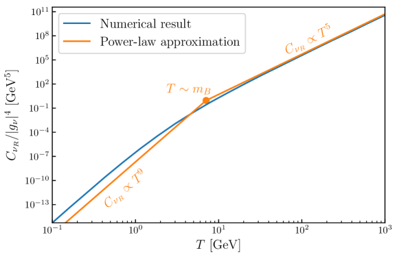
Figure 1: Power-law approximation of the collision term of $F+\overline{F}\rightarrow\nu_{R}+\overline{\nu_{R}}$ compared with the numerical (exact) result. In this illustration, the approximate curve is produced according to Eq. (49) with $N_{\nu_{R}}=1$, $m_{B}=10$ GeV and $m_{F}=0.1$ GeV. The numerical result is obtained using the method in Appendix B with the same values, assuming $B$ is a scalar and initial/final particles obey Fermi-Dirac statistics.

Eqs. (45) and (49) are our power-law approximations of collision terms for decay and annihilation processes, respectively. Since we have used several approximations in the derivation, it should only be an estimation of the order of magnitude. In Fig. 1, we compare our power-law approximation of the collision term for subcase (III-2) with the exact result which is obtained using the method introduced in Appendix B.

IV.2 Approximate result

With the power-law approximations of collision terms in Eqs. (45) and (49), we are ready to approximately estimate the abundance of $\nu_{R}$ using the integral in Eq. (41). The Hubble parameter is determined by $H^{2}=8\pi\rho_{{\rm tot}}/(3m_{{\rm pl}}^{2})$, where $\rho_{{\rm tot}}$ is the total energy density and $m_{{\rm pl}}=1.22\times 10^{19}$ GeV is the Planck mass. We take $\rho_{{\rm tot}}\approx\rho_{{\rm SM}}$ in the Hubble parameter so that

$$H\approx\sqrt{\frac{8\pi^{3}g_{\star}^{(\rho)}}{90}}\frac{T^{2}}{m_{{\rm pl}}}.$$ (50)

In the SM entropy density,

$$s_{{\rm SM}}(T)=\frac{2\pi^{2}}{45}g_{\star}^{(s)}T^{3},$$ (51)

we neglect the small difference between $g_{\star}^{(s)}$ and $g_{\star}^{(\rho)}$, and use $g_{\star}\approx g_{\star}^{(s)}\approx g_{\star}^{(\rho)}$. In addition, we treat $g_{\star}$ as a constant inside the integral. When we compute the derivative $s_{{\rm SM}}^{\prime}(T)$ and the integral, the mean value $\langle g_{\star}\rangle$ is used instead of $g_{\star}$.

For the following power-law form of $C_{\nu_{R}}$,

$$C_{\nu_{R}}(T)\approx\Lambda^{n-1}T^{6-n},\ (n>0),$$ (52)

the integral in Eq. (41) converges for $T\rightarrow\infty$. This can be seen from power counting: $s_{{\rm SM}}\sim T^{3}$, $s_{{\rm SM}}^{\prime}\sim T^{2}$, $H\sim T^{2}$, $C_{\nu_{R}}s_{{\rm SM}}^{\prime}/(Hs_{{\rm SM}}^{7/3})\sim 1/T^{n+1}$. To make the integral $\int^{\infty}\frac{1}{T^{n+1}}dT$ converge for $T\rightarrow\infty$, we need $n>0$. Therefore, in the freeze-in mechanism when $T$ increases to sufficiently large vales, $C_{\nu_{R}}$ should increase slower than $T^{6}$. Indeed, one can see that both Eqs. (45) and (49) satisfy this requirement.

Substituting Eqs. (45) and (49-51) in Eq. (41), we obtain

$$\frac{\rho_{\nu_{R}}}{\rho_{{\rm SM}}}\sim N_{\nu_{R}}S|{\cal M}|^{2}\frac{15\sqrt{5}g_{\star}^{1/3}m_{\text{pl}}}{16\pi^{13/2}\langle g_{\star}\rangle^{11/6}}\times\begin{cases}T^{-3}&\ \ (T\gtrsim m_{1}/3)\\ (m_{1}/3)^{-3}&\ \ (T\lesssim m_{1}/3)\end{cases},\ {\rm for\ }B/F\ {\rm decay},$$ (53)

and

$$\frac{\rho_{\nu_{R}}}{\rho_{{\rm SM}}}\sim N_{\nu_{R}}|g_{\nu}|^{4}\frac{45\sqrt{5}g_{\star}^{1/3}m_{\text{pl}}}{64\pi^{17/2}\langle g_{\star}\rangle^{11/6}}\begin{cases}\frac{1}{T}&\ \frac{m_{X}}{\sqrt{2}}\lesssim T\\[5.69054pt] \frac{4\sqrt{2}}{3m_{X}}-\frac{4T^{3}}{3m_{X}^{4}}&\ \frac{m_{1}}{3}\lesssim T\lesssim\frac{m_{X}}{\sqrt{2}}\\[5.69054pt] \frac{4\sqrt{2}}{3m_{X}}-\frac{4m_{1}^{3}}{81m_{X}^{4}}&\ T\lesssim\frac{m_{1}}{3}\end{cases},\ {\rm for\ }B/F\ {\rm annihilation}.$$ (54)

Note that $g_{\star}=g_{\star}(T)$ is a $T$-dependent quantity and $\langle g_{\star}\rangle$ is the effective mean value used in the integral. As an approximation, one can take $\langle g_{\star}\rangle\sim g_{\star}(T=m_{X})$ in Eq. (54) or $\langle g_{\star}\rangle\sim g_{\star}(T=m_{1})$ in Eq. (53), because $\nu_{R}$ is the most efficiently produced at this temperature.

We further translate the results of $\rho_{\nu_{R}}/\rho_{{\rm SM}}$ into $\Delta N_{{\rm eff}}$ according to Eq. (8), which results in

$$\Delta N_{{\rm eff}}\sim 2.7\frac{m_{\text{pl}}S|{\cal M}|^{2}}{\langle g_{\star}\rangle^{11/6}m_{1}^{3}}\sim 0.1\times\left(\frac{100}{\langle g_{\star}\rangle}\right)^{11/6}\left(\frac{700\ {\rm GeV}}{m_{1}}\right)\left|\frac{g_{\nu}}{10^{-7}}\right|^{2},$$ (55)

for $B$ or $F$ decay, and

$$\Delta N_{{\rm eff}}\sim 1.4\times 10^{-2}\frac{m_{\text{pl}}|g_{\nu}|^{4}}{\langle g_{\star}\rangle^{11/6}m_{X}}\sim 0.1\times\left(\frac{100}{\langle g_{\star}\rangle}\right)^{11/6}\left(\frac{400\ {\rm GeV}}{m_{X}}\right)\left|\frac{g_{\nu}}{10^{-3}}\right|^{4},$$ (56)

for $B$ or $F$ annihilation.

Eqs. (55) and (56) are our final results for the approximate estimation. Here $m_{1}$ is the initial particle mass and $m_{X}$ is $m_{F}$ for case (II-2) and $m_{B}$ for case (III-2). We stress that the results presented here are based on several approximations which might deviate from the exact result by one or even two orders of magnitude—see Fig. 1 for example. The results should only be used to qualitatively estimate the order of magnitude. In particular, since we ignored the back-reaction, it would be incorrect to apply Eqs. (55) and (56) to large $\Delta N_{{\rm eff}}$ due to saturated production rates. If the freeze-in process happens at temperatures well above the electroweak scale and $\nu_{R}$ has been decoupled since then, we know that $\Delta N_{{\rm eff}}$ should be smaller than 0.14 Abazajian:2019oqj ; Luo:2020sho . This provides a useful criterion to check whether the back-reaction can be neglected or not.

In the next section, we will discuss an example in which our approximate result is compared with the exact one, namely when Dirac neutrino masses are generated by the SM Higgs mechanism.

V The SM Higgs as an example

Let us assume neutrinos are Dirac particles and their masses originate from tiny Yukawa couplings with the SM Higgs (flavor indices are ignored here),

$${\cal L}\supset Y_{\nu}\overline{L}\tilde{H}\nu_{R},$$ (57)

where $L=(\nu_{L},\ e_{L})^{T}$, $\tilde{H}=i\sigma_{2}H^{*}$ and $H=\frac{1}{\sqrt{2}}(0,v+h)^{T}$ in the unitary gauge. Here $h$ is the Higgs boson and $v\approx 246$ GeV. Eq. (57) gives rise to neutrino masses $m_{\nu}=\frac{v}{\sqrt{2}}Y_{\nu}$, which implies that the Yukawa couplings should be

$$Y_{\nu}=\sqrt{2}\frac{m_{\nu}}{v}=5.7\times 10^{-13}\left(\frac{m_{\nu}}{0.1\ {\rm eV}}\right).$$ (58)

In the unitary gauge $\nu_{R}$ couples to the SM only via ${\cal L}\supset\frac{Y_{\nu}}{\sqrt{2}}h\overline{\nu_{L}}\nu_{R}$. According to our discussion in Sec. II, the dominant process for $\nu_{R}$ production is Higgs decay: $h\rightarrow\nu_{R}+\overline{\nu}_{L}$. According to Tab. LABEL:tab:Dominant-processes, the squared amplitude is

$$|{\cal M}|^{2}=\frac{1}{2}Y_{\nu}^{2}m_{h}^{2},$$ (59)

where $m_{h}\approx 125$ GeV is the Higgs mass. In the Maxwell-Boltzmann (MB) approximation, the collision term of $h\rightarrow\nu_{R}+\overline{\nu}_{L}$ can be computed analytically according to Appendix A—see also Ref. Escudero:2020dfa . The result reads:

$$C_{\nu_{R}}\approx N_{\nu_{R}}|{\cal M}|^{2}\frac{m_{h}^{2}}{64\pi^{3}}TK_{2}\left(\frac{m_{h}}{T}\right),\ \ {\rm(MB\ approximation}),$$ (60)

where $K_{2}$ is a $K$-type Bessel function of order $2$. Since $K_{2}(x)\approx 2x^{-2}$ for $x\ll 1$ and $K_{2}(x)\sim e^{-x}$ for $x\gg 1$, Eq. (60) is approximately consistent with the power-law approximation in Eq. (45).

To obtain the exact result using Bose-Einstein and Fermi-Dirac distributions, one has to invoke Monte-Carlo integration, which is detailed in Appendix B. In Fig. 2, we present the results obtained from exact numerical calculations and the aforementioned approximations (MB and power-law).

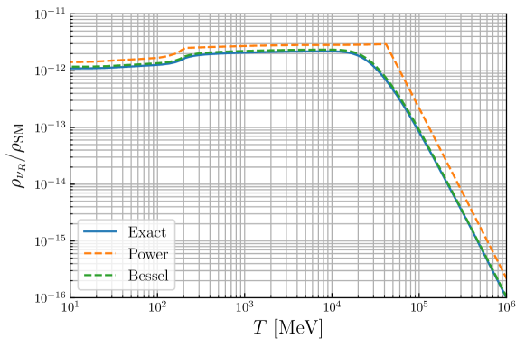
Figure 2: The SM Higgs as an example. Taking the Yukawa coupling in Eq. (58), we compute the effect of the Higgs-$\nu_{R}$-$\nu_{L}$ coupling on the $\nu_{R}$ abundance in the early Universe and obtain $\Delta N_{{\rm eff}}\approx 7.5\times 10^{-12}$. The blue curve is obtained by numerically solving the Boltzmann equation and invoking Monte-Carlo integration of the phase space. The orange curve is obtained using the power-law approximation—see Eq. (53). The green curve assumes Maxwell-Boltzmann statistics, so that the collision term can be analytically formulated as a Bessel function in Eq. (60).

Taking the low-temperature value of the blue curve in Fig. 2 and using Eq. (8), we obtain

$$\Delta N_{{\rm eff}}\approx 7.5\times 10^{-12}\left(\frac{m_{\nu}}{0.1\ {\rm eV}}\right)^{2}.$$ (61)

This is a precise result on $\Delta N_{{\rm eff}}$ that originates from the SM Higgs interaction with Dirac neutrinos.

VI Numerical approach

In this section, we numerically solve the Boltzmann equations (3) and (6) to investigate the evolution of the $\nu_{R}$ abundance for all cases outlined in Tab. LABEL:tab:Dominant-processes. Although solving the differential equation itself is not difficult, computing the collision term $C_{\nu_{R}}$ which is a 9- or 12-dimensional integral is computationally expensive. In some simple cases, the collision term is analytically calculable assuming that all thermal species obey the Maxwell-Boltzmann statistics. Known examples include decay of a massive particle to two massless particles (used in Section V) and $2\rightarrow 2$ scattering of four massless particles with contact interactions. The analytical expressions can be derived following the calculations in Appendix A of Ref. Dolgov:1997mb and Appendix D of Ref. Fradette:2018hhl , and the results can be found, e.g., in Appendix A of this paper (for $1\rightarrow 2$) or Appendix C in Ref. Luo:2020sho (for $2\rightarrow 2$). More complicated collision terms with Fermi-Dirac/Bose-Einstein statistics and/or with more massive states and/or with and non-contact interactions, can only be evaluated accurately via numerical approaches.

For numerical evaluation of high-dimensional integrals, usually one has to adopt the Monte-Carlo method. Monte-Carlo integration of multi-particle phase space is often used in collider phenomenology studies and has been implemented in a variety of packages including CalcHEP Belyaev:2012qa and similar other tools. However, since the Monte-Carlo module in CalcHEP is more dedicated to calculations of cross sections, in order to compute the collision terms more conveniently and efficiently, we develop our own Monte-Carlo module using similar techniques to that in Appendix I of the CalcHEP manual. The details are presented in Appendix B. As aforementioned, for both $1\rightarrow 2$ and $2\rightarrow 2$ processes, there are special cases with known analytical results. We have checked that our Monte-Carlo module can accurately reproduce those results.

It it important to note that when the $\nu_{R}$ temperature $T_{\nu_{R}}$ is much smaller than the SM temperature $T$, the collision term $C_{\nu_{R}}(T,\ T_{\nu_{R}})$, as a function of $T$ and $T_{\nu_{R}}$, is almost exclusively determined by $T$, i.e., $C_{\nu_{R}}(T,\ T_{\nu_{R}})\approx C_{\nu_{R}}(T,\ 0)$. When $T_{\nu_{R}}$ is approaching $T$, in order to take the back-reaction into account, we use

$$C_{\nu_{R}}(T,\ T_{\nu_{R}})\approx C_{\nu_{R}}(T,\ 0)-C_{\nu_{R}}(T_{\nu_{R}},\ 0),$$ (62)

which, as we have numerically checked, turns out to be a rather accurate approximation. Note that $C_{\nu_{R}}(T,\ T_{\nu_{R}})$ constructed in this way satisfies the condition of thermal equilibrium: $C_{\nu_{R}}(T,\ T_{\nu_{R}})=0$ when $T=T_{\nu_{R}}$. Furthermore, this treatment can be justified from analytical results as well. Taking subcase (III-2) for example, we know that when $m_{F}\ll T\ll m_{B}$ there is an analytical result: $C_{\nu_{R}}\propto T^{9}-T_{\nu_{R}}^{9}$ Luo:2020sho , which indeed can be decomposed in the form of Eq. (62).

We comment here that when $\nu_{R}$ is not in thermal equilibrium, the temperature $T_{\nu_{R}}$ is not well defined. Actually particles produced by freeze-in usually have non-thermal distributions very different from the Fermi-Dirac one (see e.g. Bae:2017dpt ; Ballesteros:2020adh ). Nevertheless, we find that in our case using the Fermi-Dirac distribution for $\nu_{R}$ causes very little deviation from the true value because the shapes of $f_{3}$ and $f_{4}$ affect the result mainly via the backreaction term which is negligible when $\rho_{\nu_{R}}$ is small. When $\rho_{\nu_{R}}$ saturates the upper bound of thermal equilibrium, it enters the freeze-out regime where the Fermi-Dirac distribution with a well-defined $T_{\nu_{R}}$ can be used. Only in a quite narrow window when $\rho_{\nu_{R}}/\rho_{\nu_{L}}$ is approaching $1$ (i.e. in the transition from the freeze-in to freeze-out regimes), the specific form of backreaction matters. We leave possible refinements in this window to future work.

By applying the Monte-Carlo procedure to each process in Tab. LABEL:tab:Dominant-processes with the assumption of Eq. (62), we obtain the numerical values of the collision terms which will be passed to the differential equation solver to solve $\rho_{\nu_{R}}$. Theoretically, the Boltzmann equations should be solved starting from the initial point at $T=\infty$ with $\rho_{\nu_{R}}=0$. According to our power-law analyses in Sec. IV, if we set the initial point at a finite $T$ with $\rho_{\nu_{R}}=0$, the deviation $\delta\rho_{\nu_{R}}$ from the true value is

$$\delta\rho_{\nu_{R}}/\rho_{\nu_{R}}\sim\begin{cases}{\cal O}(m_{B,F}^{3}/T^{3})&{\rm\ for\ decay}\\ {\cal O}(m_{B,F}/T)&{\rm\ for\ annihilation}\end{cases},$$ (63)

where $m_{B,F}=\max(m_{B},\ m_{F})$. Therefore to limit the error within, e.g., $1\%$, one only needs to set $T>{\cal O}(10^{2}\,m_{B,F})$.

Last, we note that the Boltzmann equations (3) and (6) can be combined as

$$\frac{d\rho_{\nu_{R}}}{d\rho_{{\rm SM}}}=\frac{4H\rho_{\nu_{R}}-C_{\nu_{R}}^{(\rho)}}{3H(\rho_{{\rm SM}}+P_{{\rm SM}})+C_{\nu_{R}}^{(\rho)}}.$$ (64)

We use Eq. (64) to avoid involving the time parameter $t$ for the sake of stability of the Boltzmann equation solver. Occasionally (when $\nu_{R}$ is strongly coupled to the SM plasma), we use ${dT_{\nu_{R}}}/{dT_{{\rm SM}}}$ instead of ${d\rho_{\nu_{R}}}/{d\rho_{{\rm SM}}}$ and impose an upper bound $T_{\nu_{R}}\leq T_{\rm SM}$ in the Boltzmann equation solver.

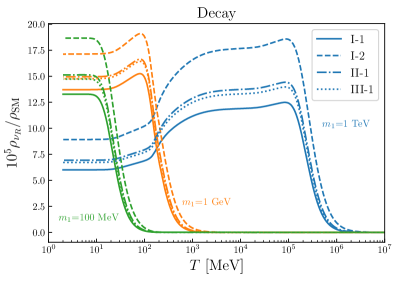
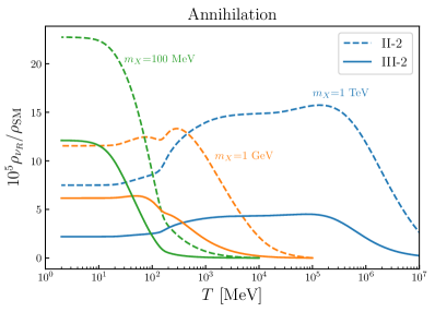
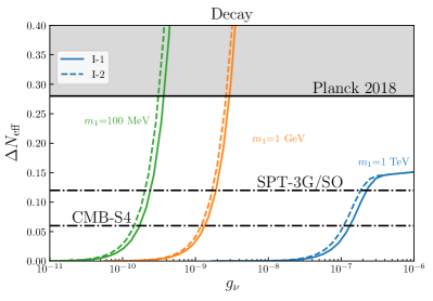
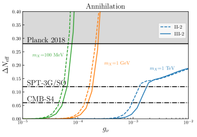
Figure 3: Upper panels: the energy density of right-handed neutrinos $\rho_{\nu_{R}}$ obtained by numerically solving the Boltzmann equations (3) and (6) for all cases listed in Tab. LABEL:tab:Dominant-processes. Lower panels: contributions of $\nu_{R}$ to $N_{{\rm eff}}$ for varying $g_{\nu}$. Here $m_{1}$ is the initial particle mass of the decay process and $m_{X}$ is the internal propagator mass of the annihilation process. Other relevant parameters are specified in the text.

In the upper panels of Fig. 3 we present the solutions obtained from Eq. (64) for several selected samples for decay (left) and annihilation (right) processes. The former includes four subcases: (I-1), (I-2), (II-1) and (III-1); and the later includes two subcases: (II-2) and (III-2). Their collision terms are computed according to Eq. (62) with $C_{\nu_{R}}(T,\ 0)$ given as follows:

$$C_{\nu_{R}}^{\textrm{(I-1)}}(T,\ 0) = S|{\cal M}|^{2}\int d\Pi_{1}d\Pi_{3}d\Pi_{4}\frac{E_{3}}{e^{E_{1}/T}-1}\left[1-\frac{1}{e^{E_{4}/T}+1}\right](2\pi)^{4}\delta^{4},$$ (65)

$$C_{\nu_{R}}^{\textrm{(I-2)}}(T,\ 0) = S|{\cal M}|^{2}\int d\Pi_{1}d\Pi_{3}d\Pi_{4}\frac{E_{3}}{e^{E_{1}/T}+1}\left[1+\frac{1}{e^{E_{4}/T}-1}\right](2\pi)^{4}\delta^{4},$$ (66)

$$C_{\nu_{R}}^{\textrm{(II-1)}}(T,\ 0) = S|{\cal M}|^{2}\int d\Pi_{1}d\Pi_{3}d\Pi_{4}\frac{E_{3}}{e^{E_{1}/T}-1}(2\pi)^{4}\delta^{4},$$ (67)

$$C_{\nu_{R}}^{\textrm{(III-1)}}(T,\ 0) = S|{\cal M}|^{2}\int d\Pi_{1}d\Pi_{3}d\Pi_{4}\frac{E_{3}}{e^{E_{1}/T}+1}(2\pi)^{4}\delta^{4},$$ (68)

$$C_{\nu_{R}}^{\textrm{(II-2)}}(T,\ 0) = \int d\Pi_{1}d\Pi_{2}d\Pi_{3}d\Pi_{4}\frac{(2\pi)^{4}\delta^{4}E_{3}S|{\cal M}|^{2}}{\left(e^{E_{1}/T}-1\right)\left(e^{E_{2}/T}-1\right)},$$ (69)

$$C_{\nu_{R}}^{\textrm{(III-2)}}(T,\ 0) = \int d\Pi_{1}d\Pi_{2}d\Pi_{3}d\Pi_{4}\frac{(2\pi)^{4}\delta^{4}E_{3}S|{\cal M}|^{2}}{\left(e^{E_{1}/T}+1\right)\left(e^{E_{2}/T}-1\right)}.$$ (70)

Here $\delta^{4}$ is short for $\delta^{4}(p_{1}-p_{3}-p_{4})$ or $\delta^{4}(p_{1}+p_{2}-p_{3}-p_{4})$. For $S|{\cal M}|^{2}$, we take the scalar results from Tab. LABEL:tab:Dominant-processes. Note that despite $S|{\cal M}|^{2}$ being the same for subcases (I-1) and (II-1), or for subcases (I-2) and (III-1), the above expressions of $C_{\nu_{R}}$ for these cases are different. The initial particle mass, $m_{1}$, should be either $m_{F}$ or $m_{B}$, as already specified in Tab. LABEL:tab:Dominant-processes for each subcase. We select in Fig. 3 three representative values of $m_{1}$: 1 TeV, 1 GeV, and 100 MeV, with $g_{\nu}=10^{-8}$ ($2.8\times 10^{-4})$, $1.6\times 10^{-10}$ ($4.4\times 10^{-5}$), and $2\times 10^{-11}$ ($1.8\times 10^{-5}$) in the left (right) panel, respectively. In Fig. 3, we set $m_{F}=0$ if $m_{F}<m_{B}$ or $m_{B}=0$ if $m_{B}<m_{F}$; the effect of nonzero $m_{F}$ or $m_{B}$ is shown in Fig. 4.

In the lower panels of Fig. 3, we show the contribution to $N_{\rm eff}$ according to Eqs. (8) or (9) as a function of $g_{\nu}$ with $m_{F}$ and $m_{B}$ being the same as in the upper panel. Results for subcases (II-1) and (III-1) are not presented in the lower left panel because, as already suggested by the upper left panel, they would be in between subcases (I-1) and (I-2). We confront the results with current and future experimental bounds on $\Delta N_{\rm eff}$ from Planck 2018 Akrami:2018vks ; Aghanim:2018eyx , the Simons Observatory (SO) Abitbol:2019nhf , the South Pole Telescope (SPT-3G) Benson:2014qhw , and CMB-S4 Abazajian:2016yjj ; Abazajian:2019eic . The Planck 2018 measurement gives $N_{{\rm eff}}=2.99\pm 0.17$ (1$\sigma$) which after subtracting the $\nu_{L}$ contribution ($2.99-3.045=-0.055$) is recast as $\Delta N_{{\rm eff}}<0.17\times 2-0.055=0.285$ at 2$\sigma$ C.L. The SO and SPT-3G sensitivities are similar ($\Delta N_{{\rm eff}}<0.12$ at 2$\sigma$ C.L.), labeled together as SO/SPT-3G. Finally, the future CMB-S4 limit is expected to reach 0.06, also at 2$\sigma$ C.L.

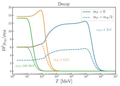
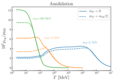
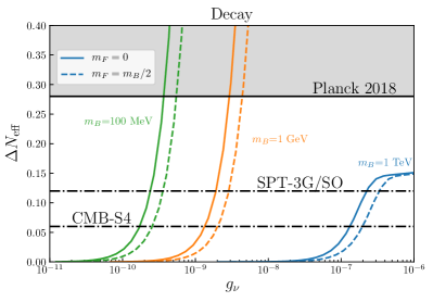
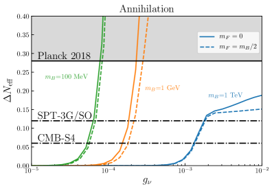
Figure 4: Similar to Fig. 3 but in order to illustrate the effect of $\min(m_{F},\,m_{B})\neq 0$, we compare curves of $m_{F}=m_{B}/2$ with $m_{F}=0$, assuming subcases (I-1) and (III-2) in the left and right panels, respectively. Other relevant parameters are specified in the text.

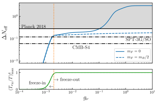
Figure 5: Transition from the freeze-in to freeze-out regimes when $g_{\nu}$ increases to sufficiently large values. The shown example takes $m_{B}=1$ TeV in subcase (III-2). In the lower panel, the maximal temperature ratio $(T_{\nu_{R}}/T)^{4}_{\max}$ indicates whether $\nu_{R}$ had been in thermal equilibrium. In the upper panel, the two plateaus at $\Delta N_{\rm eff}\approx 0.14$ and $\Delta N_{\rm eff}\approx 3$ correspond to $\nu_{R}$ decoupling above the electroweak scale and around the MeV scale, respectively. The latter does not exist for the dashed curve because with $m_{F}=m_{B}/2$, the collision term becomes exponentially suppressed below the electroweak scale—see the text for more discussions.

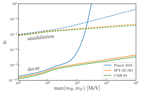
Figure 6: Upper bounds on $g_{\nu}$ obtained from the requirement that $\Delta N_{{\rm eff}}$ does not exceed the current measurement of Planck 2018 Akrami:2018vks ; Aghanim:2018eyx or the sensitivity of future CMB experiments including SO Abitbol:2019nhf , SPT-3G Benson:2014qhw , and CMB-S4 Abazajian:2016yjj ; Abazajian:2019eic .

As shown in Fig. 3, for decay processes the production of $\nu_{R}$ is most efficient when the temperature is lower than the initial particle mass $m_{1}$. Typically most $\nu_{R}$ are produced within $0.1m_{1}\lesssim T\lesssim m_{1}$. For annihilation processes, the production is most efficient around $T\sim m_{X}$, the mass of the internal particle in the process. After that, the $\rho_{\nu_{R}}/\rho_{\rm SM}$ curves would remain stable if the composition of the SM plasma was not changed. However, at low temperatures due to many heavy SM species annihilating or decaying into light ones, the comoving energy density of SM increases and hence $\rho_{\nu_{R}}/\rho_{\rm SM}$ decreases when $\nu_{R}$ is no longer effectively produced. The most significant decrease in the curve appears during 100 MeV $\lesssim T\lesssim 1$ GeV, where $g_{\star}$ becomes substantially smaller. This feature holds for GeV or TeV masses, for lighter particles $\nu_{R}$ has not been produced yet in significant amounts.

The differences between dashed and solid curves in Fig. 3 are caused by differences of $C_{\nu_{R}}$ in Eqs. (65)-(70), or more specifically, by the difference between Fermi-Dirac and Bose-Einstein statistics. The “$\pm$” and “$\mp$” signs in Eqs (4) and (5) can lead to enhancement or suppression of $\rho_{\nu_{R}}$ by a factor of $R$ with $R\lesssim 1.5$ (decay) or $R\lesssim 4$ (annihilation). Consequently, the effect on $\Delta N_{\rm eff}$-$g_{\nu}$ in the lower panels is approximately a horizontal shift by a factor of $R^{1/2}$ (decay) or $R^{1/4}$ (annihilation) because in the freeze-in mechanism we have $\Delta N_{\rm eff}\propto g_{\nu}^{2}$ and $\Delta N_{\rm eff}\propto g_{\nu}^{4}$ for decay and annihilation processes respectively. The effect of nonzero $\min(m_{B},\,m_{F})$ is quite similar, as shown in Fig. 4. Taking subcases (I-1) and (III-2) as examples, in which $m_{B}$ is assumed to be larger than $m_{F}$, we plot curves for both $m_{F}=m_{B}/2$ and $m_{F}=0$. The difference can be accounted for also by the $R$ factor which is typically around 2 or 3, leading to a $R^{1/2}$ or $R^{1/4}$ horizontal shift of the $\Delta N_{\rm eff}$-$g_{\nu}$ curves. Note that the case of $m_{F}=0$ could correspond to $F$ being the left-handed component of the Dirac neutrinos.

Here we comment on a noteworthy behavior of large $g_{\nu}$ when $m_{X}$, the propagator mass in the annihilation case, is above the electroweak scale. For sufficiently large $g_{\nu}$, $\nu_{R}$ can reach thermal equilibrium at a temperature well above the electroweak scale. If the initial particle mass $m_{1}=\min(m_{B},\,m_{F})$ is also above the electroweak scale, then at a lower (yet still above the electroweak scale) temperature $\nu_{R}$ will leave thermal equilibrium because the collision term is exponentially suppressed at $T\ll m_{1}$. Therefore, in this case, $\nu_{R}$ reaches and leaves thermal equilibrium at temperatures above the electroweak scale, leading to a constant $\Delta N_{\rm eff}\approx 0.14$ Abazajian:2019oqj ; Luo:2020sho . If $m_{1}$ is below the electroweak scale, the decoupling temperature generally depends on $g_{\nu}$. As shown by the blue dashed and solid curve in the lower right panel in Fig. 4, larger $g_{\nu}$ may or may not increase $\Delta N_{\rm eff}$, depending on whether $m_{1}$ is below or above the electroweak scale.

In Fig. 5, we further explore the dependence of $\Delta N_{\rm eff}$ on even larger $g_{\nu}$. Here we take subcase (III-2) with $m_{B}=1$ TeV and $m_{1}=m_{F}=\{0,m_{B}/2\}$. For more general values of $m_{1}$ below the electroweak scale, the result would be between the blue solid and dashed curves. As has been expected, for larger $g_{\nu}$, the blue solid curve further increases and eventually reaches the maximal value ($\Delta N_{\rm eff}=3$) that $\nu_{R}$ could produce (in this case we assume $F$ is $\nu_{L}$); while the blue dashed curve is insensitive to $g_{\nu}$, approximately keeping a constant value of $\Delta N_{\rm eff}$ at 0.14.

Fig. 5 also shows explicitly the transition of the freeze-in to freeze-out regimes. Actually, for strong couplings $\nu_{R}$ had been in thermal equilibrium, thus its relic abundance depends on how late it would decouple from the SM plasma rather than how fast it was initially produced. As indicated by the lower panel, $(T_{\nu_{R}}/T)^{4}_{\max}$, defined as the maximal value of $(T_{\nu_{R}}/T)^{4}$ during the entire evolution, reaches $1$ when $g_{\nu}\gtrsim 2\times 10^{-3}$ (the orange dashed line). This is a good measure for the transition from the freeze-in to the freeze-out regime.

Finally, by requiring that the contribution of $\nu_{R}$ to $N_{\rm eff}$ does not exceed the current limit or future sensitivities of the aforementioned CMB experiments, we can obtain upper bounds on $g_{\nu}$. They are presented in Fig. 6, where we select subcases (I-1) and (III-2) for the decay and annihilation curves, respectively. Here we set $\min(m_{B},\ m_{F})=0$ and $\max(m_{B},\ m_{F})\geq 10^{2}$ MeV. The latter is to ensure that the calculation is not affected by $\nu_{L}$ decoupling. As previously discussed, for decay processes most $\nu_{R}$ are produced within $0.1\lesssim T/\max(m_{B},\ m_{F})\lesssim 1$. For $\min(m_{B},\ m_{F})=0$, we assume that $B$ and $F$ do not contribute to $\Delta N_{{\rm eff}}$ significantly (e.g. $F$ may be $\nu_{L}$). One can also set $\min(m_{B},\ m_{F})$ to 10 MeV for example to suppress their contributions to $\Delta N_{{\rm eff}}$. This causes very insignificant changes in the final results. As we have demonstrated in Figs. 3 and 4, selecting other cases or using nonzero values of $\min(m_{B},m_{F})$ typically increases or reduces $\Delta N_{\rm eff}$ by a factor of $R\approx 2\sim 4$ and hence the bounds on $g_{\nu}$ by a factor of $R^{1/2}$ or $R^{1/4}$. However, since the Planck 2018 limit on $\Delta N_{\rm eff}$ is above 0.14, for large masses the bounds can be weakened drastically and become more mass dependent. In fact, if $\nu_{R}$ production and decoupling (if it ever reached thermal equilibrium) are all well beyond the electroweak scale (this leads to $\Delta N_{\rm eff}\leq 0.14$), Planck 2018 cannot provide a valid constraint on it. For the SO/SPT-3G and CMB-S4 curves, because these future experiments will be probing the freeze-in regime for large masses, the curves will not be significantly changed if nonzero values of $\min(m_{B},m_{F})$ are used. Generally, we can draw the conclusion that for $\max(m_{B},m_{F})<1$ GeV, the current CMB measurement excludes $g_{\nu}\gtrsim 10^{-9}$ or $g_{\nu}\gtrsim 10^{-3}$ via the decay or annihilation processes, respectively. For larger masses, the Planck 2018 bounds are more mass-dependent (depending on both $\min(m_{B},m_{F})$ and $\max(m_{B},m_{F})$), while the SO/SPT-3G and CMB-S4 bounds mainly depend on $\max(m_{B},m_{F})$, where power-law extrapolations according to Eqs. (55) and (56) can be used.

VII Conclusion

Dirac neutrinos with new interactions can have a measurable effect on the effective number of relativistic neutrino species $N_{\rm eff}$ in the early Universe, courtesy of a possible thermalization of the right-handed components $\nu_{R}$. We have computed here the effect of new vector and scalar interactions of right-handed neutrinos with new bosons and chiral fermions. Various special cases of this framework exist, depending on which particle is in equilibrium and which one is heavier, see Tab. LABEL:tab:Dominant-processes. We focused on freeze-in of the right-handed neutrinos, and confronted the results with present and upcoming precise determinations of $\Delta N_{\rm eff}$.

Approximate analytical results are given in Eqs. (55) and (56); the outcome of a numerical solutions of the relevant equations is given in Figs. 3 to 6. For instance, if decay (scattering) of new particles is the dominating freeze-in process, limits on the new coupling constants of order $10^{-4}$ ($10^{-9}$) may be constrained for new particle masses around GeV. Chiral fermions being in equilibrium and massless can correspond to SM neutrinos. This also allows to consider the case of Dirac neutrino masses generated by the SM Higgs mechanism, which gives (see Fig. 2) $\Delta N_{\rm eff}^{\rm SM}\approx 7.5\times 10^{-12}\,(m_{\nu}/(0.1\,{\rm eV}))^{2}$.

The results of this paper cover a wide range of possibilities, and demonstrate once more that cosmological measurements can constrain fundamental properties of particle physics, in particular neutrino physics.

Appendix A Analytical results of 3-particle phase space integrals

Since in many $1\rightarrow 2$ processes the squared amplitudes $|{\cal M}|^{2}$ are energy-independent, it is useful to present the analytical results of the following integrals:

$$I^{(n)} \equiv \int d\Pi_{1}d\Pi_{3}d\Pi_{4}(2\pi)^{4}\delta^{4}(p_{1}-p_{3}-p_{4})e^{-E_{1}/T},$$ (71)

$$I^{(\rho)} \equiv \int d\Pi_{1}d\Pi_{3}d\Pi_{4}(2\pi)^{4}\delta^{4}(p_{1}-p_{3}-p_{4})e^{-E_{1}/T}E_{3},$$ (72)

where $m_{1}\neq 0$ and $m_{3}=m_{4}=0$.

The results are

$$I^{(n)} \equiv \frac{1}{32\pi^{3}}m_{1}TK_{1}\left(\frac{m_{1}}{T}\right),$$ (73)

$$I^{(\rho)} \equiv \frac{1}{64\pi^{3}}m_{1}^{2}TK_{2}\left(\frac{m_{1}}{T}\right),$$ (74)

where $K_{1}$ and $K_{2}$ are $K$-type Bessel functions of order $1$ and $2$ respectively. Next we derive these two analytical results.

First, we substitute $(2\pi)^{3}\delta^{3}(\boldsymbol{p}_{1}-\boldsymbol{p}_{3}-\boldsymbol{p}_{4})=\int e^{i(\boldsymbol{p}_{1}-\boldsymbol{p}_{3}-\boldsymbol{p}_{4})\cdot\boldsymbol{\lambda}}d^{3}\boldsymbol{\lambda}$ and $d\Pi_{i}=\frac{p_{i}^{2}dp_{i}d\Omega_{i}}{(2\pi)^{3}2E_{i}}$ in Eqs. (71) and (72):

$$I\equiv\frac{1}{(2\pi)^{9}}\int\frac{p_{1}^{2}dp_{1}}{2E_{1}}\frac{p_{3}^{2}dp_{3}}{2E_{3}}\frac{p_{4}^{2}dp_{4}}{2E_{4}}2\pi\delta(E_{1}-p_{3}-p_{4})e^{-E_{1}/T}UI_{\Omega},$$ (75)

where $U=E_{3}$ for $I^{(\rho)}$ or $1$ for $I^{(n)}$, and $I_{\Omega}$ contains the angular part of the integral:

$$I_{\Omega} = \int d^{3}\boldsymbol{\lambda}\int d\Omega_{1}e^{i\boldsymbol{p}_{1}\cdot\boldsymbol{\lambda}}\int d\Omega_{3}e^{-i\boldsymbol{p}_{3}\cdot\boldsymbol{\lambda}}\int d\Omega_{4}e^{-i\boldsymbol{p}_{4}\cdot\boldsymbol{\lambda}}.$$ (76)

Since $\int d\Omega_{i}e^{\pm i\boldsymbol{p}_{i}\cdot\boldsymbol{\lambda}}=\int dc_{i}d\phi_{i}e^{\pm ip_{i}\lambda c_{i}}=4\pi\frac{\sin(p_{i}\lambda)}{p_{i}\lambda}$, we further get

$$I_{\Omega} = (4\pi)^{3}\int d^{3}\boldsymbol{\lambda}\frac{\sin(p_{1}\lambda)}{p_{1}\lambda}\frac{\sin(p_{3}\lambda)}{p_{3}\lambda}\frac{\sin(p_{4}\lambda)}{p_{4}\lambda}$$ (77)

$$= (4\pi)^{4}\int_{0}^{\infty}\frac{d\lambda}{p_{1}p_{3}p_{4}\lambda}\sum_{\eta_{1},\eta_{3},\eta_{4}}\frac{-\eta_{1}\eta_{3}\eta_{4}}{8}\sin\left(\eta_{1}p_{1}\lambda+\eta_{3}p_{3}\lambda+\eta_{4}p_{4}\lambda\right)$$

$$= \frac{32\pi^{5}}{p_{1}p_{3}p_{4}}\left[\frac{p_{1}-p_{3}+p_{4}}{|p_{1}-p_{3}+p_{4}|}+\frac{p_{1}+p_{3}-p_{4}}{|p_{1}+p_{3}-p_{4}|}-\frac{p_{1}-p_{3}-p_{4}}{|p_{1}-p_{3}-p_{4}|}-\frac{p_{1}+p_{3}+p_{4}}{|p_{1}+p_{3}+p_{4}|}\right],$$

where in the second line $\eta_{i}=\pm 1$ denotes positive/negative signs, and in the last line we have used $\int\frac{d\lambda}{\lambda p}\sin(\lambda p)=1/|p|$.

Using Eq. (77), it is straightforward to integrate out $p_{3}$ and $p_{4}$ in Eq. (75), leading to

$$I^{(n)} = \frac{1}{(2\pi)^{9}}\int\frac{16\pi^{6}p_{1}^{2}}{E_{1}}e^{-E_{1}/T}dp_{1}=\frac{1}{32\pi^{3}}\int_{m_{1}}^{\infty}p_{1}e^{-E_{1}/T}dE_{1},$$ (78)

$$I^{(\rho)} = \frac{1}{(2\pi)^{9}}\int 8\pi^{6}p_{1}^{2}e^{-E_{1}/T}dp_{1}=\frac{1}{64\pi^{3}}\int_{m_{1}}^{\infty}p_{1}E_{1}e^{-E_{1}/T}dE_{1}.$$ (79)

The above integrals can be expressed in terms of the Bessel functions, as already given in Eqs. (73) and (74).

Appendix B Monte-Carlo integration of general collision terms

In this appendix, we introduce the techniques we use to numerically evaluate the phase space integrals of collision terms. The method is based on Monte-Carlo integration and in principle applies to any $m\rightarrow n$ ($m$, $n=$1, 2, 3,$\cdots$) processes.

Consider the following integral

$$I[{\cal F}]\equiv\int d\Pi_{1}d\Pi_{2}\cdots d\Pi_{m+n}(2\pi)^{4}\delta^{4}(p_{1}+p_{2}+\cdots p_{m}-p_{m+1}-\cdots p_{m+n}){\cal F}(p_{1},\ p_{2},\ \cdots),$$ (80)

where $p_{1}$, $p_{2}$, $\cdots$, $p_{m}$ ($p_{m+1}$, $\cdots$, $p_{m+n}$) are momenta of initial (final) particles,

$$d\Pi_{i}=\frac{d^{3}p_{i}}{(2\pi)^{3}2E_{i}},$$ (81)

and ${\cal F}$ is a general function of all the momenta. For simplicity, we denote $p_{1}+p_{2}+\cdots p_{m}-p_{m+1}-\cdots-p_{m+n-2}$ by $q$, and the last two momenta $p_{m+n}$ and $p_{m+n-1}$ by $p_{\bar{1}}$ and $p_{\bar{2}}$, respectively.

There are two technical problems in the Monte-Carlo integration that we need to deal with properly, otherwise the Monte-Carlo integration would converge very slowly. The first one concerns the $\delta$ function, which will be removed by integrating out some part of the momenta. The second problem is that the integration domain is infinitely large, which can be avoided by a proper transformation of variables.

To remove the $\delta$ function, we first integrate out $\boldsymbol{p}_{\bar{1}}$ so that

$$I=\int d\Pi_{1}d\Pi_{2}\cdots d\Pi_{m+n-1}\frac{2\pi}{2E_{\bar{1}}}\delta(E_{q}-E_{\bar{2}}-E_{\bar{1}}){\cal F},$$ (82)

where $E_{q}$, $E_{\bar{2}}$ and $E_{\bar{1}}$ are the energies of the on-shell momenta $q$, $p_{\bar{1}}$ and $p_{\bar{2}}$, respectively. Note that since $\boldsymbol{p}_{\bar{1}}$ has already been integrated out in Eq. (82), instead of being a function of $\boldsymbol{p}_{\bar{1}}$, $E_{\bar{1}}$ should be interpreted as a function of $\boldsymbol{q}$ and $\boldsymbol{p}_{\bar{2}}$:

$$E_{\bar{1}}=\sqrt{m_{\bar{1}}^{2}+|\boldsymbol{q}-\boldsymbol{p}_{\bar{2}}|^{2}}.$$ (83)

Next, we integrate out $|\boldsymbol{p}_{\bar{2}}|$ in Eq. (82) and obtain

$$I=\int d\Pi_{1}d\Pi_{2}\cdots d\Pi_{m+n-2}\frac{|\boldsymbol{p}_{\bar{2}}|^{2}dc_{\bar{2}}d\phi_{\bar{2}}}{(2\pi)^{3}2E_{\bar{2}}}\frac{2\pi}{2E_{\bar{1}}}J^{-1}{\cal F}\Theta,$$ (84)

where $c_{\bar{2}}=\cos\theta_{\bar{2}}$, $\theta_{\bar{2}}$ and $\phi_{\bar{2}}$ are the polar and azimuthal angles in a spherical coordinate system with the zenith direction aligned with $\boldsymbol{q}$ (hence $\boldsymbol{p}_{\bar{2}}\cdot\boldsymbol{q}=|\boldsymbol{p}_{\bar{2}}||\boldsymbol{q}|c_{\bar{2}}$), and

$$J^{-1}=\left|\frac{\partial(E_{\bar{2}}+E_{\bar{1}})}{\partial|\boldsymbol{p}_{\bar{2}}|}\right|^{-1}=\left|\frac{|\boldsymbol{p}_{\bar{2}}|}{E_{\bar{2}}}+\frac{|\boldsymbol{p}_{\bar{2}}|-|\boldsymbol{q}|c_{\bar{2}}}{E_{\bar{1}}}\right|^{-1},$$ (85)

according to the property of $\delta$ function: $\delta(g(x))=\delta(x-x_{0})\left|g^{\prime}(x_{0})\right|^{-1}$ with $x_{0}$ being a root of $g(x_{0})=0$.

The Heaviside theta function $\Theta$ takes either 1 or 0 depending on whether $q^{\mu}$ and $c_{\bar{2}}$ lead to physical kinematics or not. Technically, it is computed as follows:

$$\Theta=\begin{cases}1&{\rm if}\ q^{2}>(m_{\bar{1}}+m_{\bar{2}})^{2}\ \&\ \Delta>0\\ 0&{\rm otherwise}\end{cases}\,,$$ (86)

where

$$\Delta\equiv m_{\bar{2}}^{4}+\left(m_{\bar{1}}^{2}-q^{2}\right){}^{2}-2m_{\bar{2}}^{2}\left[q^{2}+2\left(1-c_{\bar{2}}^{2}\right)|\boldsymbol{q}|^{2}+m_{\bar{1}}^{2}\right].$$ (87)

Note that in the above expression $q^{2}=E_{q}^{2}-|\boldsymbol{q}|^{2}$ is different from $|\boldsymbol{q}|^{2}$. The condition $q^{2}>(m_{\bar{1}}+m_{\bar{2}})^{2}$ enforces that $q$ provides sufficient energy to generate particles $\bar{2}$ and $\bar{1}$. This can be derived in the center-of-mass frame of particles $\bar{2}$ and $\bar{1}$, where $\boldsymbol{q}=0$ and it is obvious that near the threshold both particles should be almost at rest. Slightly above the threshold, we need $E_{q}$ to be slightly larger than $m_{\bar{1}}+m_{\bar{2}}$ to produce the two particles. So in the center-of-mass frame, $E_{q}>m_{\bar{1}}+m_{\bar{2}}$ is necessary and sufficient for $q$ to produce the two particles. In other frames with nonzero values of $|\boldsymbol{q}|$, by applying a Lorentz transformation, we get $q^{2}-(m_{\bar{1}}+m_{\bar{2}})^{2}>0$. The other requirement $\Delta>0$ puts a further constraint on the angles, which will be derived in Eq. (89).

Next, we need to reconstruct $\boldsymbol{p}_{\bar{2}}$ from given values of $E_{q}$, $\boldsymbol{q}$, and $\theta_{\bar{2}}$. In principle, $|\boldsymbol{p}_{\bar{2}}|$ in Eq. (84) should be interpreted as an implicit function of these quantities and $\phi_{\overline{2}}$. However, $\phi_{\overline{2}}$ turns out to be irrelevant here.

Given $E_{q}$, $\boldsymbol{q}$, and $c_{\bar{2}}$, $|\boldsymbol{p}_{\bar{2}}|$ is determined by

$$E_{q}=\sqrt{m_{\bar{2}}^{2}+|\boldsymbol{p}_{\bar{2}}|^{2}}+\sqrt{m_{\bar{1}}^{2}+|\boldsymbol{q}-\boldsymbol{p}_{\bar{2}}|^{2}},$$ (88)

which can be solved as a quadratic equation of $|\boldsymbol{p}_{\bar{2}}|$ and gives

$$|\boldsymbol{p}_{\bar{2}}|=\frac{c_{\bar{2}}|\boldsymbol{q}|\left(q^{2}-m_{\bar{1}}^{2}+m_{\bar{2}}^{2}\right)+E_{q}\sqrt{\Delta}}{2\left(E_{q}^{2}-c_{\bar{2}}^{2}|\boldsymbol{q}|^{2}\right)}.$$ (89)

Eq. (89) implies that $\Delta$ cannot be negative otherwise Eq. (88) would have no real solution. This sets a constraint on $c_{\bar{2}}$. As can be seen from Eq. (87), for a fixed value of $q^{2}$, one can boost $|\boldsymbol{q}|^{2}$ to an arbitrarily large value so that the $\left(1-c_{\bar{2}}^{2}\right)|\boldsymbol{q}|^{2}$ term is dominant and leads to $\Delta<0$, unless $1-c_{\bar{2}}^{2}$ is suppressed. So generally speaking, for very large $|\boldsymbol{q}|^{2}$ and nonzero $m_{\bar{2}}^{2}$, the physically allowed region for $1-c_{\bar{2}}^{2}$ is small. This feature could be used to improve the the efficiency of Monte-Carlo integration by limiting the sampling space of $c_{\bar{2}}^{2}$, though it has not been implemented in our code.

Once $|\boldsymbol{p}_{\bar{2}}|$ is determined from Eq. (89), we can readily compute $E_{\bar{2}}$, $E_{\bar{1}}$, and $|\boldsymbol{p}_{\bar{1}}|$.

The second problem concerns the infinitely large domain of integration (each $|\boldsymbol{p}_{i}|$ is integrated from 0 to $\infty$). We make the following variable transformation for each $|\boldsymbol{p}_{i}|$:

$$x_{i}\equiv\exp\left(-|\boldsymbol{p}_{i}|/\Lambda_{i}\right),\ \ {\rm or}\ \ |\boldsymbol{p}_{i}|=-\Lambda_{i}\log(x_{i}),$$ (90)

and integrate $x_{i}$ from 0 to 1. In our code we usually take $\Lambda_{i}=4T_{i}$, which usually leads to efficient convergence of the Monte-Carlo integration. The transformation also generates another Jacobian:

$$J_{i}\equiv dx_{i}/dp_{i}=-x_{i}/\Lambda\,,$$ (91)

which should be included in the integration via $dp_{i}\rightarrow dx_{i}/J_{i}$.

In summary, the Monte-Carlo integration of $I$ can be implemented as follows:

• Randomly generate values of $(x_{i},\ c_{i},\ \phi_{i})$ with $i=1,\cdots,n+m-2$, $x_{i}\in(0,\ 1)$, $c_{i}\in(-1,\ 1)$, and $\phi_{i}\in(0,\ 2\pi)$;

• Construct the spatial parts of the first $n+m-2$ momenta ($\boldsymbol{p}_{1}$, $\boldsymbol{p}_{2}$, $\cdots$, $\boldsymbol{p}_{n+m-2}$) from $(x_{i},\ c_{i},\ \phi_{i})$;

• Compute their respective energies $E_{1},E_{2},\cdots,E_{n+m-2}$ according to the on-shell condition;

• Construct $q=(E_{q},\ \boldsymbol{q})$ with $E_{q}=\sum_{i=1}^{n+m-2}E_{i}$ and $\boldsymbol{q}=\sum_{i=1}^{n+m-2}\boldsymbol{p}_{i}$;

• Randomly generate $c_{\bar{2}}$ and $\phi_{\bar{2}}$ in Eq. (84);

• Compute $|\boldsymbol{p}_{\bar{2}}|$ according to Eq. (89) so that the second last momentum $p_{\bar{2}}=(E_{\bar{2}},\ \boldsymbol{p}_{\bar{2}})$ can be reconstructed;

• Reconstruct the last momentum according to $p_{\bar{1}}=q-p_{\bar{2}}$;

• Evaluate the integrand in Eq. (84) and proceed with the standard Monte-Carlo procedure. Note that in addition to the Jacobian in Eq. (85), there is also another Jacobian $J_{i}$ in Eq. (91) that needs to be included.

B.1 Example: $1\rightarrow 2$ processes

As the simplest example, let us apply the above method to $1\rightarrow 2$ processes,

$$I\equiv\int d\Pi_{1}d\Pi_{2}d\Pi_{3}(2\pi)^{4}\delta^{4}(p_{1}-p_{2}-p_{3}){\cal F}(p_{1},\ p_{2},\ p_{3})\,.$$ (92)

Following the above notation, the $q$ momentum is identical to $p_{1}$ and hence $q^{2}=m_{1}^{2}$ which implies that in the $\Theta$ function the $q^{2}>(m_{2}+m_{3})^{2}$ condition (equivalent to $m_{1}>m_{2}+m_{3}$) can be ignored. The integral is computed as follows:

$$I=\left\langle\frac{|\boldsymbol{p}_{1}|^{2}}{(2\pi)^{3}2E_{1}}\frac{|\boldsymbol{p}_{2}|^{2}}{(2\pi)^{3}2E_{2}}\frac{2\pi}{2E_{3}}J^{-1}J_{1}{\cal F}\Theta\right\rangle V,$$ (93)

where $\langle\rangle$ stands for the mean value after a large number of evaluations of the inside quantity, $J_{1}$ is given in Eq. (91), and $V=1\times 2^{2}\times(2\pi)^{2}$ is the volume of the sampling space: $x_{1}\in(0,\ 1)$, $c_{1,2}\in(-1,\ 1)$, $\phi_{1,2}\in(0,\ 2\pi)$. Let us apply the the Monte-Carlo method to Eq. (72), which has a known analytical result. Taking $T=m_{1}=1$ GeV and assuming other particles are massless, the Bessel-form expression in Eq. (72) gives $I=8.188\times 10^{-4}\ {\rm GeV}^{3}$. Performing the Monte-Carlo evaluation of Eq. (93) with $10^{7}$ samples for ten times, we get $I/(10^{-4}\ {\rm GeV}^{3})=$ {8.196, 8.197, 8.203, 8.190, 8.164, 8.174, 8.186, 8.176, 8.195, 8.185}, which is consistent with the analytical result. Each evaluation with $10^{7}$ samples takes about three seconds using our code currently implemented in Python.

B.2 Example: $2\rightarrow 2$ processes

Consider a $2\rightarrow 2$ process with the kinematics $p_{1}+p_{2}=p_{3}+p_{4}$ and $q=p_{1}+p_{2}$. In this case, we have

$$I=\int d\Pi_{1}d\Pi_{2}\frac{|\boldsymbol{p}_{3}|^{2}dc_{3}d\phi_{3}}{(2\pi)^{3}2E_{3}}\frac{2\pi}{2E_{4}}J^{-1}{\cal F}\Theta,$$ (94)

where ${\cal F}$ contains statistical distribution functions and a scattering amplitude. The scattering amplitude usually can be expressed in terms of $p_{1}\cdot p_{2}$, $p_{1}\cdot p_{3}$ and $p_{2}\cdot p_{3}$. If it contains scalar products of $p_{4}$, then we can replace $p_{4}$ with $p_{1}+p_{2}-p_{3}$. For example, $p_{1}\cdot p_{4}$ can be written as $p_{1}\cdot(p_{1}+p_{2}-p_{3})=m_{1}^{2}+p_{1}\cdot p_{2}-p_{1}\cdot p_{3}$.

To facilitate the calculation of scalar products, it would be better to define all the polar angles (i.e. $\theta$’s) with respective to $\boldsymbol{q}$. But since $\boldsymbol{q}$ is constructed from $\boldsymbol{p}_{1}$ and $\boldsymbol{p}_{2}$, such definitions would be conceptually confusing. We perform the variable transformation: $(\boldsymbol{p}_{1},\ \boldsymbol{p}_{2})\rightarrow(\boldsymbol{q},\ \boldsymbol{p}_{2})=(\boldsymbol{p}_{1}+\boldsymbol{p}_{2},\ \boldsymbol{p}_{2})$ to avoid this confusion. Since the Jacobian of this transformation is $1$, after the transformation Eq. (94) becomes

$$I=\int\frac{|\boldsymbol{q}|^{2}d|\boldsymbol{q}|dc_{q}d\phi_{q}}{(2\pi)^{3}2E_{q}}\frac{|\boldsymbol{p}_{2}|^{2}d|\boldsymbol{p}_{2}|dc_{2}d\phi_{2}}{(2\pi)^{3}2E_{2}}\frac{|\boldsymbol{p}_{3}|^{2}dc_{3}d\phi_{3}}{(2\pi)^{3}2E_{3}}\frac{2\pi}{2E_{4}}J^{-1}{\cal F}\Theta,$$ (95)

where $c_{2}=\cos\theta_{2}$ and $\theta_{2}$ is defined as the angle between $\boldsymbol{p}_{2}$ and $\boldsymbol{q}$.

With the proper definition of $c_{2}$ (similar to $c_{3}$), we have

$$q\cdot p_{2}=E_{q}E_{2}-|\boldsymbol{q}||\boldsymbol{p}_{2}|c_{2},\ \ q\cdot p_{3}=E_{q}E_{3}-|\boldsymbol{q}||\boldsymbol{p}_{3}|c_{3},$$ (96)

and

$$p_{2}\cdot p_{3}=E_{2}E_{3}-|\boldsymbol{p}_{2}||\boldsymbol{p}_{3}|\left[s_{2}s_{3}\cos(\phi_{2}-\phi_{3})+c_{2}c_{3}\right],$$ (97)

where $(s_{2},\ s_{3})\equiv(\sin\theta_{2},\ \sin\theta_{3})$. From Eqs. (96) and (97), it is straightforward to obtain any scalar products of $p_{1}$, $p_{2}$, $p_{3}$, and $p_{4}$.

It is also known that in the MB approximation, the collision terms of contact interactions of four massless fermions are analytically calculable. For example, given

$${\cal F}=\exp(-E_{1}/T)\exp(-E_{2}/T)(p_{1}\cdot p_{2})(p_{3}\cdot p_{4}),$$ (98)

the analytical result is (see Tab. III in Ref. Luo:2020sho ):

$$I=\frac{3T^{8}}{8\pi^{5}}\approx 1.225\times 10^{-3}\ T^{8}.$$ (99)

Performing the Monte-Carlo integration described above with $10^{6}$ samples, we find that the numerical factor typically varies from $1.22\times 10^{-3}$ to $1.23\times 10^{-3}$, which is in agreement with the analytical result.

References

- (1) KATRIN Collaboration, M. Aker et al., Improved Upper Limit on the Neutrino Mass from a Direct Kinematic Method by KATRIN, Phys. Rev. Lett. 123 (2019), no. 22 221802, [1909.06048].
- (2) M. J. Dolinski, A. W. Poon, and W. Rodejohann, Neutrinoless Double-Beta Decay: Status and Prospects, Ann. Rev. Nucl. Part. Sci. 69 (2019) 219–251, [1902.04097].
- (3) G. Steigman, K. A. Olive, and D. Schramm, Cosmological Constraints on Superweak Particles, Phys. Rev. Lett. 43 (1979) 239–242.
- (4) K. A. Olive, D. N. Schramm, and G. Steigman, Limits on New Superweakly Interacting Particles from Primordial Nucleosynthesis, Nucl. Phys. B180 (1981) 497–515.
- (5) A. D. Dolgov, Neutrinos in cosmology, Phys. Rept. 370 (2002) 333–535, [hep-ph/0202122].
- (6) D. Borah, B. Karmakar, and D. Nanda, Common Origin of Dirac Neutrino Mass and Freeze-in Massive Particle Dark Matter, JCAP 07 (2018) 039, [1805.11115].
- (7) K. N. Abazajian and J. Heeck, Observing Dirac neutrinos in the cosmic microwave background, Phys. Rev. D 100 (2019) 075027, [1908.03286].
- (8) S. Jana, V. P. K., and S. Saad, Minimal dirac neutrino mass models from gauge symmetry and left–right asymmetry at colliders, Eur. Phys. J. C 79 (2019), no. 11 916, [1904.07407].
- (9) J. Calle, D. Restrepo, and O. Zapata, Dirac neutrino mass generation from a Majorana messenger, Phys. Rev. D 101 (2020), no. 3 035004, [1909.09574].
- (10) X. Luo, W. Rodejohann, and X.-J. Xu, Dirac neutrinos and , JCAP 06 (2020) 058, [2005.01629].
- (11) D. Borah, A. Dasgupta, C. Majumdar, and D. Nanda, Observing left-right symmetry in the cosmic microwave background, Phys. Rev. D 102 (2020), no. 3 035025, [2005.02343].
- (12) P. Adshead, Y. Cui, A. J. Long, and M. Shamma, Unraveling the Dirac Neutrino with Cosmological and Terrestrial Detectors, 2009.07852.
- (13) C. Boehm, M. J. Dolan, and C. McCabe, Increasing Neff with particles in thermal equilibrium with neutrinos, JCAP 1212 (2012) 027, [1207.0497].
- (14) A. Kamada and H.-B. Yu, Coherent Propagation of PeV Neutrinos and the Dip in the Neutrino Spectrum at IceCube, Phys. Rev. D92 (2015), no. 11 113004, [1504.00711].
- (15) P. F. de Salas and S. Pastor, Relic neutrino decoupling with flavour oscillations revisited, JCAP 07 (2016) 051, [1606.06986].
- (16) A. Kamada, K. Kaneta, K. Yanagi, and H.-B. Yu, Self-interacting dark matter and muon in a gauged U model, JHEP 06 (2018) 117, [1805.00651].
- (17) M. Escudero, Neutrino decoupling beyond the Standard Model: CMB constraints on the Dark Matter mass with a fast and precise evaluation, JCAP 1902 (2019) 007, [1812.05605].
- (18) P. F. Depta, M. Hufnagel, K. Schmidt-Hoberg, and S. Wild, BBN constraints on the annihilation of MeV-scale dark matter, JCAP 1904 (2019) 029, [1901.06944].
- (19) C. Lunardini and Y. F. Perez-Gonzalez, Dirac and Majorana neutrino signatures of primordial black holes, JCAP 2008 (2020) 014, [1910.07864].
- (20) M. Escudero Abenza, Precision Early Universe Thermodynamics made simple: and Neutrino Decoupling in the Standard Model and beyond, 2001.04466.
- (21) Planck Collaboration, N. Aghanim et al., Planck 2018 results. I. Overview and the cosmological legacy of Planck, Astron. Astrophys. 641 (2020) A1, [1807.06205].
- (22) Planck Collaboration, N. Aghanim et al., Planck 2018 results. VI. Cosmological parameters, Astron. Astrophys. 641 (2020) A6, [1807.06209].
- (23) SPT-3G Collaboration, B. Benson et al., SPT-3G: A Next-Generation Cosmic Microwave Background Polarization Experiment on the South Pole Telescope, Proc. SPIE Int. Soc. Opt. Eng. 9153 (2014) 91531P, [1407.2973].
- (24) Simons Observatory Collaboration, M. H. Abitbol et al., The Simons Observatory: Astro2020 Decadal Project Whitepaper, Bull. Am. Astron. Soc. 51 (2019) 147, [1907.08284].
- (25) CMB-S4 Collaboration, K. N. Abazajian et al., CMB-S4 Science Book, First Edition, 1610.02743.
- (26) K. Abazajian et al., CMB-S4 Science Case, Reference Design, and Project Plan, 1907.04473.
- (27) L. J. Hall, K. Jedamzik, J. March-Russell, and S. M. West, Freeze-In Production of FIMP Dark Matter, JHEP 03 (2010) 080, [0911.1120].
- (28) G.-y. Huang, T. Ohlsson, and S. Zhou, Observational Constraints on Secret Neutrino Interactions from Big Bang Nucleosynthesis, Phys. Rev. D97 (2018), no. 7 075009, [1712.04792].
- (29) M. Berbig, S. Jana, and A. Trautner, The Hubble tension and a renormalizable model of gauged neutrino self-interactions, 2004.13039.
- (30) H.-J. He, Y.-Z. Ma, and J. Zheng, Resolving Hubble Tension by Self-Interacting Neutrinos with Dirac Seesaw, JCAP 11 (2020) 003, [2003.12057].
- (31) B. Wallisch, Cosmological Probes of Light Relics. PhD thesis, Cambridge U., 2018. 1810.02800.
- (32) L. Husdal, On Effective Degrees of Freedom in the Early Universe, Galaxies 4 (2016), no. 4 78, [1609.04979].
- (33) H. H. Patel, Package-X: A Mathematica package for the analytic calculation of one-loop integrals, Comput. Phys. Commun. 197 (2015) 276–290, [1503.01469].
- (34) A. Dolgov, S. Hansen, and D. Semikoz, Nonequilibrium corrections to the spectra of massless neutrinos in the early universe, Nucl. Phys. B 503 (1997) 426–444, [hep-ph/9703315].
- (35) A. Fradette, M. Pospelov, J. Pradler, and A. Ritz, Cosmological beam dump: constraints on dark scalars mixed with the Higgs boson, Phys. Rev. D99 (2019), no. 7 075004, [1812.07585].
- (36) A. Belyaev, N. D. Christensen, and A. Pukhov, CalcHEP 3.4 for collider physics within and beyond the Standard Model, Comput. Phys. Commun. 184 (2013) 1729–1769, [1207.6082].
- (37) K. J. Bae, A. Kamada, S. P. Liew, and K. Yanagi, Light axinos from freeze-in: production processes, phase space distributions, and Ly- forest constraints, JCAP 1801 (2018) 054, [1707.06418].
- (38) G. Ballesteros, M. A. G. Garcia, and M. Pierre, How warm are non-thermal relics? Lyman- bounds on out-of-equilibrium dark matter, 2011.13458.