Unusually thick metal-insulator domain walls around the Mott point

Abstract

Many Mott systems feature a first-order metal-insulator transition at finite temperatures, with an associated phase coexistence region displaying inhomogeneities and local phase separation. Here one typically finds “bubbles” or domains of the respective phases, which are separated by surprisingly thick, or fat, domain walls, as revealed both by imaging experiments and recent theoretical modeling. To gain insight into this unexpected behavior, we perform a systematic model study of the structure of such metal-insulator domain walls around the Mott point, within the Dynamical Mean-Field Theory framework. Our study reveals that a mechanism producing such “fat” domain walls can be traced to strong magnetic frustration, which is expected to be a robust feature of “spin-liquid” Mott systems.

I Introduction

The Mott (interaction-driven) metal-insulator transition represents one of the most important phenomena in strongly correlated electron systems.Mott (1990) It was first recognized in a number of transition-metal oxides,Lederer et al. (1972); McWhan et al. (1973); Mazzaferro et al. (1980); Limelette et al. (2003); Qazilbash et al. (2007) and has been brought to notoriety with the discovery of the cuprate high-$T_{c}$ superconductors,Patrick A. Lee et al. (2006); Cai, P. et al. (2016) which raised much controversy surrounding its character and the underlying physical processes. One popular viewpoint, going back to early ideas of Slater, assumes that the key mechanism producing the Mott insulating state follows from magnetic order simply rearranging the band structure. An alternative perspective, pioneered by the seminal ideas of Mott and Anderson, argues that strong Coulomb repulsion may arrest the electronic motion even in the absence of magnetic order. Several theoretical scenarios Hubbard (1957, 1958); Brinkman and Rice (1970); A. Georges et al. (1996) have been proposed for the vicinity of the Mott point, but for many years the controversy remained unresolved.

More recent experiments have demonstrated Kurosaki et al. (2005) that a sharp Mott transition is indeed possible even in the absence of any magnetic order. Physically, this possibility is realized in systems where sufficiently strong magnetic frustrationPowell and McKenzie (2011) can suppress magnetic order down to low enough temperatures, thus revealing the “pure” Mott point. Precisely such behavior is found in a class $\kappa$-organic “spin-liquid” materials,Dressel and Tomic (2020) which have been recently recognizedVollhardt (2020) as the ideal realization of a single-band Hubbard model on a triangular lattice, allowing a remarkably detailed insight into the Mott transition region. While the intermediate-temperature metal-insulator crossover revealedFurukawa et al. (2015) some striking aspects of quantum criticalityH. Terletska et al. (2011) around the quantum Widom line, Vučičević et al. (2013); Pustogow et al. (2018) the transition was found to assume weakly first-order character at the lowest temperatures. Spectacular anomalies in dielectric response were observedPustogow et al. (2021) within the associated phase coexistence region, revealing percolative phase separation.

Remarkably, most qualitative and even semi-quantitative aspects of the behaviorDressel and Tomic (2020) observed around the Mott point were found to validate the predictions of Dynamical Mean-Field Theory (DMFT). Pruschke et al. (1995); A. Georges et al. (1996) This theoretical approach, which gained considerable popularity in recent years,Kotliar and Vollhardt (2004) focuses on the local effects of strong Coulomb repulsion, while disregarding certain nonlocal processes associated with inter-site magnetic correlations and/or fluctuating magnetic orders. It reconciled the earlier theories of HubbardHubbard (1957, 1958) with the viewpoint of Brinkman and Rice,Brinkman and Rice (1970) leading to a consistent non-perturbative picture of the Mott point.

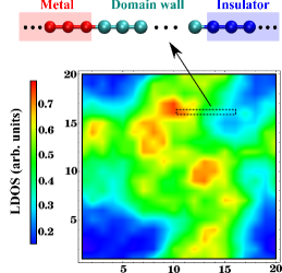
Figure 1: Spatial fluctuations of the local density of states (LDOS) found in a recent simulation of a moderately disordered two-dimensional Mott system, within the metal-insulator phase coexistence region.M. Y. Suárez-Villagrán et al. (2020) Note how the domain walls (green) covers a substantial area of the image, separating metallic (red) from the Mott-insulating domains (blue). Similar patterns have also been found in earlier imaging experiments on certain Mott oxides.Qazilbash et al. (2007)

While many aspects of crystalline Mott materials prove to be successfully described and interpreted from the perspective of DMFT, the situation is more complicated in the presence of disorder,Miranda and Dobrosavljević (2005); Tanasković et al. (2003); Dobrosavljević et al. (2003); M. C. O. Aguiar et al. (2004); Aguiar et al. (2005, 2009); Andrade et al. (2009, 2010) which breaks translational invariance. These effects are most pronounced, but least understood, within the metal-insulator phase coexistence region. Here even moderate disorder creates nucleation centers for the respective phases, leading to nano-scale phase separation. Some aspects of this behavior proved possible to be described from the perspective of a phenomenological percolation picture, including the effects of inhomogeneities caused by thermal fluctuations around the critical end-point,Papanikolaou et al. (2008) as well as the colossal dielectric response at lower temperatures.Pustogow et al. (2021)

A closer look at the microscopic structure of the corresponding patterns, however, revealed various puzzling features. Hints of remarkably complex behavior were provided by very recent large-scale numerical modelingM. Y. Suárez-Villagrán et al. (2020) of disordered Mott systems, as well as experimentally by nano-scale imaging of some Mott materials.Qazilbash et al. (2007) A typical situation is illustrated in Fig. 1, where we reproduce a result of our recent theoretical studyM. Y. Suárez-Villagrán et al. (2020) of this regime. Here we see clearly defined metallic domains separated from Mott-insulating regions by surprisingly thick domain walls, which in some cases cover a large fraction of the system volume (area). Remarkably, very similar fat domain walls were also observed in certain experiments,Qazilbash et al. (2007) suggesting robust new physics. This finding immediately brings into question the conventional percolation picture, where the domain walls are assumed to play only a secondary role. This observation also brings forth several important physical questions, which are the primary motivation for this work: (1) What is the physical reason for having rather thick or fat domain walls, and under which conditions is this expected to hold? (2) What are the physical properties of such “domain wall matter”, and how should they affect the physical observables?

In this study we present a detailed theoretical investigation of the structure of such domain walls not only in the vicinity to the critical end-pointLee and Yee (2017) (where one generally expects them to be thick), but also across the entire phase-coexistence region. Our results establish that, under certain conditions, such domain walls can remain thick in the entire range of temperatures, and reveal the underlying mechanism, at least within the DMFT picture we adopt. We argue that strong magnetic frustration acts as a key physical ingredient affecting the properties of such domain walls, also suggesting ways to further control their properties in “materials by design”.Adler et al. (2018)

II Model and method

To microscopically investigate metal-insulator domain walls in the vicinity of the Mott point, we focus on a single-band half-filled Hubbard model, as given by the Hamiltonian

$$H=-t\sum_{i\sigma}\left[c_{i\sigma}^{\dagger}c_{\left(i+1\right)\sigma}^{\phantom{\dagger}}+\mathrm{h.c.}\right]+U\sum_{i}\left(n_{i\uparrow}-\frac{1}{2}\right)\left(n_{i\downarrow}-\frac{1}{2}\right),$$ (1)

where $c_{i\sigma}^{\dagger}\left(c_{i\sigma}\right)$ is the creation (annihilation) operator of an electron with spin projection $\sigma$ on site $i$, $t$ is the hopping amplitude between nearest neighbors, $U$ is the on-site Coulomb repulsion, and $n_{i\sigma}=c_{i\sigma}^{\dagger}c_{i\sigma}$. We work in units such that $\hslash=k_{B}=a=1$, where $a$ is the lattice spacing. Energy will generally be given in the units of half-band width $D$, which for our half-filled situation is also the Fermi energy.

In general terms, a domain wall in $d$ dimensions is a ($d-1$)-dimensional surface separating two thermodynamic phases. To examine its basic properties, we follow a standard procedureGoldenfeld (1992) in assuming it to be flat, i.e. that its spatial variation across the wall is the only relevant one. To further simplify the calculation, we take advantage of the the well-established fact that, within the DMFT formulation we employ, the detailed form of the electronic band structure does not qualitatively affect the results.A. Georges et al. (1996); Helmes et al. (2008); Potthoff and Nolting (1999) This allows us follow the same strategy as in standard theories for domain walls, and reduce the problem to solving a one-dimensional model with appropriate boundary conditions on each end representing the respective thermodynamic phases.

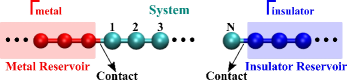
Figure 2: Schematic representation of the one-dimensional model we use to describe a domain wall. The central $N$-site sector, denoted as $H_{S}$ in the Hamiltonian, contains the domain wall. It is attached to semi-infinite leads on both sides; a uniform, strongly correlated metal on the left and a uniform Mott insulator on the right. Both these reservoirs are described by the $H_{R}$ term in the Hamiltonian. The $N$-site chain system is connected to the reservoirs through contact components, denoted as $H_{C}$ in the Hamiltonian.

To make our notation transparent, it is convenient to separate the Hamiltonian in three terms (see Fig. 2)

$$H=H_{S}+H_{R}+H_{C}.$$ (2)

The first term $H_{S}$ is a Hubbard Hamiltonian for the $N$ central sites (“system”)

$$H_{S} = -t\sum_{i=1,\sigma}^{N-1}\left[c_{i\sigma}^{\dagger}c_{\left(i+1\right)\sigma}^{\phantom{\dagger}}+\mathrm{h.c.}\right]$$ (3)

$$+U\sum_{i=1}^{N}\left(n_{i\uparrow}-\frac{1}{2}\right)\left(n_{i\downarrow}-\frac{1}{2}\right),$$

$H_{R}$ refers to the semi-infinite chains to the left and to the right of the system (“reservoirs”)

$$H_{R} = -t\left(\sum_{i=-\infty,\sigma}^{-1}+\sum_{i=N+1,\sigma}^{\infty}\right)\left[c_{i\sigma}^{\dagger}c_{\left(i+1\right)\sigma}^{\phantom{\dagger}}+\mathrm{h.c.}\right]$$ (4)

$$+U\left(\sum_{i=-\infty}^{0}+\sum_{i=N+1}^{\infty}\right)\left(n_{i\uparrow}-\frac{1}{2}\right)\left(n_{i\downarrow}-\frac{1}{2}\right),$$

and $H_{C}$ represent the coupling (“contacts”) of the central system to the reservoirs

$$H_{C}=-t\sum_{\sigma}\left[c_{0\sigma}^{\dagger}c_{1\sigma}^{\phantom{\dagger}}+c_{N\sigma}^{\dagger}c_{\left(N+1\right)\sigma}^{\phantom{\dagger}}+\mathrm{h.c.}\right].$$ (5)

In the following, we solve this model using Dynamical Mean-Field Theory (DMFT).Metzner and Vollhardt (1989); A. Georges and G. Kotliar (1992); Pruschke et al. (1995); A. Georges et al. (1996) The essential simplification of this approach is the assumption that the single-particle self-energy is a local but frequency-dependent quantity.Metzner and Vollhardt (1989) This self-energy is then calculated from the solution of an ensemble of auxiliary single-impurity problems supplemented with appropriate self-consistency conditions.A. Georges and G. Kotliar (1992) Within DMFT, the Mott transition at half-filling exhibits a coexistence region where both the metal and the insulator represent locally stable thermodynamic phases. This coexistence region is delimited in the $T$ vs. $U$ phase diagram by two spinodal lines, $U_{c1}(T)$ (where the insulator becomes unstable) and $U_{c2}(T)$ (for the instability of the metal), as shown in Fig. 3. We further concentrate on behavior along the first order transition line $U_{c}(T)$ (green line in Fig. 3) where the free energies of the respective phases become equal. H. Terletska et al. (2011); G. Moeller et al. (1999) To describe domain wall formation,Goldenfeld (1992) we impose boundary conditions such that the sites to the left of the system are in the metallic phase, whereas sites to the right of it correspond to the Mott insulator. The intermediate region will then have to smoothly interpolate between metal and insulator, thus producing a domain wall between the two phases.

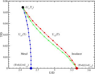
Figure 3: DMFT phase diagram for the Mott transition at half-filling, obtained using IPT as the impurity solver. The phase coexistence region is bounded by the spinodal lines $U_{c1}(T)$ (blue line) and $U_{c2}(T)$ (red line) where the respective insulating and metallic solutions become unstable. The green line marks the first order transition line $U_{c}(T)$, where the free energies of the two phases coincide.

Naturally, we will no longer be able to assume a uniform, i.e., site-independent self-energy throughout the system. We will thus generalize the assumptions of DMFT to accommodate a non-uniform albeit still site-diagonal self-energy function

$$\Sigma\left(\omega\right)\to\Sigma_{i}\left(\omega\right).$$ (6)

This approach was first proposed in the context of a disordered system in Refs. Dobrosavljević and Kotliar, 1997, 1998 (for a review, see Ref. E. Miranda and V. Dobrosavljević, 2012). In the following, we explain the details of how the self-energy is computed for the present model. Like in the homogeneous DMFT, we focus on site $i$, whose dynamics, we assume, is that of a single correlated impurity site embedded in a bath of conduction electrons, whose action in imaginary time is

$$S_{eff}\left(i\right) = \sum_{\sigma}\int_{0}^{\beta}d\tau c_{i\sigma}^{\dagger}\left(\tau\right)\left(\partial_{\tau}-U/2\right)c_{i\sigma}\left(\tau\right)$$ (7)

$$+ \sum_{\sigma}\int_{0}^{\beta}d\tau\int_{0}^{\beta}d\tau^{\prime}c_{i\sigma}^{\dagger}\left(\tau\right)\Delta_{i}\left(\tau-\tau^{\prime}\right)c_{i\sigma}\left(\tau^{\prime}\right)$$

$$+ U\int_{0}^{\beta}d\tau n_{i\uparrow}\left(\tau\right)n_{i\downarrow}\left(\tau\right).$$

The hybridization function $\Delta_{i}\left(\tau-\tau^{\prime}\right)$ describes processes whereby an electron hops out of site $i$ at time $\tau^{\prime}$, wanders through the rest of the lattice, and hops back onto $i$ at a later time $\tau$. We will specify how it is computed shortly. The local Green’s function of the impurity described by the action of Eq. (7) is

$$G_{i}\left(\tau\right)=-\left\langle T\left[c_{i\sigma}\left(\tau\right)c_{i\sigma}^{\dagger}\left(0\right)\right]\right\rangle_{eff},$$ (8)

where the subscript $eff$ emphasizes that it should be calculated under the dynamics of Eq. (7). The self-energy $\Sigma_{i}\left(i\omega_{n}\right)$ is then obtained from the Fourier transform to Matsubara frequencies

$$G_{i}\left(i\omega_{n}\right)=\frac{1}{i\omega_{n}+U/2-\Delta_{i}\left(i\omega_{n}\right)-\Sigma_{i}\left(i\omega_{n}\right)}.$$ (9)

The lattice single-particle Green’s function is given within this scheme by the resolvent (we use a hat to denote a matrix in the lattice site basis)

$$\widehat{G}\left(i\omega_{n}\right)=\left[i\omega_{n}-\widehat{H}_{0}-\widehat{\Sigma}\left(i\omega_{n}\right)\right]^{-1},$$ (10)

where $\widehat{H}_{0}$ is the non-interacting Hamiltonian [Eq. (1) with $U=0$] and the matrix elements of the self-energy operator $\widehat{\Sigma}\left(i\omega_{n}\right)$ in the site basis is

$$\left\langle i\left|\widehat{\Sigma}\left(i\omega_{n}\right)\right|j\right\rangle=\Sigma_{i}\left(i\omega_{n}\right)\delta_{ij}.$$ (11)

The self-consistency loop is closed by requiring that the site-diagonal elements of the lattice Green’s function coincide with the local Green’s functions of Eq. (8)

$$\left\langle i\left|\widehat{G}\left(i\omega_{n}\right)\right|i\right\rangle=\frac{1}{i\omega_{n}+U/2-\Delta_{i}\left(i\omega_{n}\right)-\Sigma_{i}\left(i\omega_{n}\right)}.$$ (12)

This last equation provides an expression for a self-consistent hybridization function for each site $\Delta_{i}\left(i\omega_{n}\right)$. In a completely homogeneous situation, the above scheme reduces to the standard DMFT.

The procedure described above requires the computation of the local Green’s function of Eq. (8) or, equivalently, the self-energy defined in Eq. (9) for the problem defined by the single-impurity action of Eq. (7). To this end, we utilized Iterated Perturbation Theory (IPT)A. Georges and G. Kotliar (1992); H. Kajueter and G. Kotliar (1996) as the required impurity solver. This procedure, while being computationally much more efficient than standard QMC methods, has previously been shown to properly capture both the insulating and the metallic solutions to the problem, as well as most other qualitative features of the full DMFT solution,Zhang et al. (1993) which will suffice for our purposes.

If the system size $N$ is large enough to accommodate the full extension of the domain wall, the self-energy will be practically uniform in the region of the reservoirs. In carrying out our computations for different values of $U$ and $T$, we carefully verified that this condition is satisfied. For the parameter range explored in this work, $N=50$ proved sufficient, except for the largest domain wall size we analyzed, for which a value of $N=70$ was required.

Although the system studied is infinite, the computation of the local Green’s function and self-energy in the domain wall region is all that is required, as we now explain. It is easy to see that the non-interacting Hamiltonian $\widehat{H}_{0}$ of the full infinite system has an obvious block structure given by

$$\widehat{H}_{0}=\left[\begin{array}[]{cc}\widehat{H}_{S}&\widehat{H}_{C}\\ \widehat{H}_{C}&\widehat{H}_{R}\end{array}\right].$$ (13)

Likewise, the self-energy can also be separated into system [$\widehat{\Sigma}_{S}\left(i\omega_{n}\right)$] and reservoir [$\widehat{\Sigma}_{R}\left(i\omega_{n}\right)$] blocks

$$\widehat{\Sigma}\left(i\omega_{n}\right)=\left[\begin{array}[]{cc}\widehat{\Sigma}_{S}\left(i\omega_{n}\right)&0\\ 0&\widehat{\Sigma}_{R}\left(i\omega_{n}\right)\end{array}\right].$$ (14)

The lattice Green’s function (10) satisfies the equation

$$\left[i\omega_{n}-\widehat{H}_{0}-\widehat{\Sigma}\left(i\omega_{n}\right)\right]\widehat{G}\left(i\omega_{n}\right)=\widehat{1},$$ (15)

where $\widehat{1}$ is the unit matrix. In block form, Eq. (15) reads

$$\left[\begin{array}[]{cc}i\omega_{n}-\widehat{H}_{S}-\widehat{\Sigma}_{S}\left(i\omega_{n}\right)&\widehat{H}_{C}\\ \widehat{H}_{C}&i\omega_{n}-\widehat{H}_{R}-\widehat{\Sigma}_{R}\left(i\omega_{n}\right)\end{array}\right]\left[\begin{array}[]{cc}\widehat{G}_{S}&\widehat{G}_{C}\\ \widehat{G}_{C}&\widehat{G}_{R}\end{array}\right]=\left[\begin{array}[]{cc}\widehat{1}&0\\ 0&\widehat{1}\end{array}\right],$$ (16)

which can be written out as

$$\left[i\omega_{n}-\widehat{H}_{S}-\widehat{\Sigma}_{S}\left(i\omega_{n}\right)\right]\widehat{G}_{S}+\widehat{H}_{C}\widehat{G}_{C} = \widehat{1},$$ (17)

$$\widehat{H}_{C}\widehat{G}_{S}+\left[i\omega_{n}-\widehat{H}_{R}-\widehat{\Sigma}_{R}\left(i\omega_{n}\right)\right]\widehat{G}_{C} = 0.$$ (18)

Eq. (18) can be solved to give

$$\widehat{G}_{C}=-\left[i\omega_{n}-\widehat{H}_{R}-\widehat{\Sigma}_{R}\left(i\omega_{n}\right)\right]^{-1}\widehat{H}_{C}\widehat{G}_{S},$$ (19)

and the result can be plugged into Eq. (17) to yield

$$\widehat{G}_{S} = \frac{1}{i\omega_{n}-\widehat{H}_{S}-\widehat{\Sigma}_{S}\left(i\omega_{n}\right)-\widehat{H}_{C}\left[\frac{1}{i\omega_{n}-\widehat{H}_{R}-\widehat{\Sigma}_{R}\left(i\omega_{n}\right)}\right]\widehat{H}_{C}}$$ (20)

$$\equiv \frac{1}{i\omega_{n}-\widehat{H}_{S}-\widehat{\Sigma}_{S}\left(i\omega_{n}\right)-\widehat{\Gamma}\left(i\omega_{n}\right)},$$ (21)

where

$$\widehat{\Gamma}\left(i\omega_{n}\right)=\widehat{H}_{C}\left[\frac{1}{i\omega_{n}-\widehat{H}_{R}-\widehat{\Sigma}_{R}\left(i\omega_{n}\right)}\right]\widehat{H}_{C},$$ (22)

contains all the information from the reservoirs needed for the calculation of the system’s Green’s function. Since the self-energy in the reservoirs is site-independent, we can write, for the one-dimensional lattice we are using,

$$\widehat{\Gamma}(i\omega_{n})=\widehat{\Gamma}_{L}(i\omega_{n})+\widehat{\Gamma}_{R}(i\omega_{n}),$$ (23)

where $\widehat{\Gamma}_{L(R)}\left(i\omega_{n}\right)$ is the contribution from the reservoir to the left (right) of the system. The latter quantities are given in terms of the (purely imaginary) self-energies on the left (metal) and right (insulator) $\Sigma_{L,R}\left(i\omega_{n}\right)$ as

$$\widehat{\Gamma}_{L(R)}(i\omega_{n}) = \frac{i}{2}\left\{\Omega_{L(R)}(i\omega_{n})\phantom{\sqrt{\left[\Omega_{L(R)}(i\omega_{n})\right]^{2}+4t\text{\texttwosuperior}}}\right.$$ (24)

$$\left.-\mathrm{sgn}\left(\omega_{n}\right)\sqrt{\left[\Omega_{L(R)}(i\omega_{n})\right]^{2}+4t\text{\texttwosuperior}}\right\},$$

where $\Omega_{L(R)}(i\omega_{n})=\omega_{n}-\mathrm{Im}\Sigma_{L(R)}(i\omega_{n})$.

In all our calculations we analytically continue the Matsubara Green’s functions and self-energies to the real axis using the Padé approximation.H. J. Vidberg and J. W. Serene (1977)

III Results

Next, we present the detailed results we obtained, exploring the behavior of a domain wall within the coexistence region, in the entire range of temperatures $0<T<T_{c}$, along the first-order transition line.

As we mentioned in Section II, an accurate calculation needs to make sure that the system size $N$ is large enough so that our position-dependent solution converges to the proper asymptotic limit (“reservoirs”), where the spatial variation can be ignored. To illustrate this, in Fig.4 we display the domain wall profile, as described by the spatial variation of the local density of states (DOS) $\rho(0,x)=-(1/\pi)\mathrm{Im}G(\omega=0,x)$, evaluated at $T/D=0.035$ and $U/D=2.697$, and plotted as a function of the coordinate $x$ perpendicular to the domain wall. This quantity is small in the insulator (approaching zero as $T\to 0$), but remains finite in the metal, thus displaying strong spatial variation across the domain wall. As we can see in

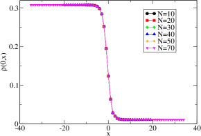
Figure 4: Spatial variation of the local DOS $\rho(0,x)$ at the Fermi energy, across the domain separating a strongly correlated metal (left) and a Mott insulator (right), corresponding to $T/D=0.0351$ and $U/D=2.69773$. Results are shown for different system sizes $N$ used in our simulation, demonstrating negligible finite-size effects of our results.

Fig.4, the spatial profile of the domain wall displays very little change with the size of the central region ($N$ sites), where we allow for spatial variation. This means that our system size $N$

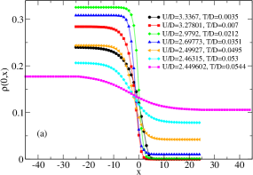
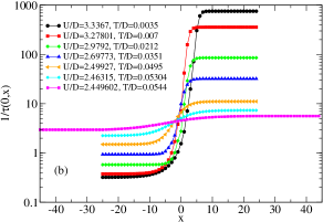
Figure 5: Variation of the domain wall profile with temperature: The local DOS (a) and the scattering rate (b) shown for different $T$ and $U$, following the first-order transition line. Note a slightly non-monotonic dependence on temperature.

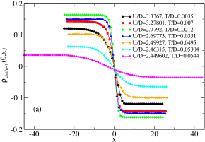
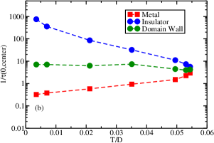
Figure 6: (a) Variation of the domain wall profile with temperature. Same data are shown in Fig. 5, but here they have been shifted both horizontally and vertically so that the domain wall center is located at the plot center. This way of plotting reveals more clearly the variation of the domain wall thickness as a function of temperature. (b) The scattering rate at the domain wall center ($x=0)$ displays very weak temperature dependence (central curve), in dramatic contrast to the behavior of either the insulator (top curve), or the metal (bottom curve) evaluated for same $T$ and $U$, along the first-order line.

is large enough to eliminate any finite-size effects from our calculation. Performing similar calculations for the different temperatures, we verified that $N=70$ is sufficient for an accurate description at all the relevant temperatures ($0<T<T_{c}$) within the coexistence region.

III.1 Anomalous dynamics of the domain walls

For each temperature we considered, we selected the precise value of $U(T)$ that falls on the first order transition line (see green line of Fig. 3). Results obtained for several temperatures are shown in Fig. 5 (a), showing the domain-wall profiles of the local DOS. We should mention that, within our simulation, the precise position of the domain wall we find for given $T$ is somewhat sensitive to the exact value for $U(T)$ selected. We had to, accordingly, adjust the value of $U$ to a precision of several decimal places, in order to obtain adequate center alignment, which is helpful for comparing the detailed form of the domain wall profile at different temperatures. For better comparison, in Fig. 6 (a) we display the same data translated along both the $x$- and the $y$-axes, so that the domain wall center coincides with the coordinate origin. Note that the local DOS in the uniform regions has a non-monotonic behavior with $T$, a behavior we expand upon in the Appendix.

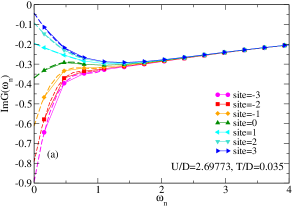
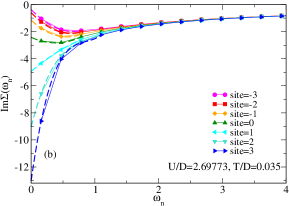
Figure 7: Domain wall central region: Matsubara frequency dependence of the imaginary part of (a) the local Green’s function and (b) the self-energy for some sites in the central portion of the domain wall at $T/D=0.035$ and $U/D=2.69773$.

The corresponding behavior of the inelastic scattering rate $1/\tau(0,x)=-2\mathrm{Im}\;\Sigma(\omega=0,x)$ across the domain wall and different temperatures is shown in Fig. 5 (b). It is generally expected to be small in a coherent metal (in a Fermi liquid $1/\tau\sim T^{2}$ for given $U$) and very large in a Mott insulator, as we observe in the respective phases. This behavior reflects a fundamentally different nature of transport in the two competing phases, but even more interesting behavior is seen within the domain wall itself. Here the scattering rate $1/\tau$ smoothly interpolates between the two limits and thus retains very weak T-dependence, reflecting significant electron-electron scattering down to the lowest temperatures! This surprising result is displayed even more precisely by plotting $1/\tau$ evaluated at the domain wall center as a function of temperature, in comparison to the behavior of the two phases, as shown in Fig. 6 (b). Similar behavior is also seen in the frequency dependence of the corresponding Green’s function and the self-energy, shown as a function of the Matsubara frequency in Fig. 7, for several sites across the domain wall at $T=0.035D$ and $U=2.698D$. Here we observe a characteristic evolution from metallic to insulating behavior, as one moves across the domain wall, which is most pronounced at the lowest frequencies. For the sites at the center of the domain wall, however, we observe characteristically weak frequency dependence. This behavior is clearly distinct from either a metal or an insulator, but is constrained by having to interpolate from one to the other.

The domain wall center is, therefore, recognized as an incoherent conductor down to the lowest temperatures. Physically, such non-Fermi liquid behavior makes it clear that the domain wall represents a different state of matter from either a coherent (Fermi liquid) metal, or a Mott insulator. This surprising result could be regarded as a curiosity with little physical consequence in situations where the relative volume (area) fraction “covered” by domain walls is negligibly small compared to the bulk of the system. In the presence of sufficient disorder, however, both recent simulationsM. Y. Suárez-Villagrán et al. (2020) and experimentsQazilbash et al. (2007) demonstrate a surprisingly abundant proliferation of such domain walls, suggesting a fundamentally new physical picture. We may expect this to be especially significant whenever the domain walls themselves are sufficiently fat (thick), so that a sizeable fraction of the system’s volume (area) is affected by such “resilient” inelastic electron-electron scattering, which persists to low temperatures, in contrast to the behavior expected for conventional metals.

III.2 What controls the thickness of the domain walls?

To precisely quantify the domain wall thickness as a function of temperature, we fit its shape to the standard $\tanh(x/\xi)$ form, generally found for domain walls separating two coexisting phases Goldenfeld (1992). To be more precise, such symmetric domain walls of thickness given by an appropriate correlation length $\xi$ is what one expects near any finite-temperature critical end-point at $T=T_{c}$, as we also find. At lower temperatures, however, our two phases are not related by any static symmetry, hence the domain wall should not necessarily retain its symmetric form, since the correlation length of the respective phases may not be exactly the same. Indeed, even a quick look at Fig. 6 (a) reveals that at lower temperatures, the domain walls are much “thicker” on the metallic than on the insulating side.

To quantify this behavior, we perform partial fits to the $\tanh(x/\xi_{a})$ form on each side of the domain wall center, which we define as the corresponding inflection point in its profile. Here $\xi_{a}$, with $a=$ $met$ or $ins$ defines the two different correlation lengths, corresponding to the respective metallic or insulating phase. The resulting $T$-dependence of $\xi_{met}$ and $\xi_{ins}$ is shown in Fig. 8 (a), together with the total domain wall thickness $\xi=(\xi_{met}+\xi_{ins})/2$. General argumentsGoldenfeld (1992) predict this quantity to diverge at $T\rightarrow T_{c}$, as we find. Indeed, the critical point at $T=T_{c}$ is known to belong to the Ising universality class Castellani et al. (1979); Rozenberg et al. (1999); Kotliar et al. (2000); Limelette et al. (2003); Papanikolaou et al. (2008); Abdel-Jawad et al. (2015). According to an appropriate Landau theoryRozenberg et al. (1999) for this critical point, the domain wall width should be proportional to the corresponding correlation length, diverging at the critical point as $\xi\sim\xi_{corr}\sim\left|T-T_{c}\right|^{1/2}.$

Remarkably, however, we find $\xi$ to display a divergence also at $T\rightarrow 0$, thus retaining a sizeable thickness even at intermediate temperatures. This behavior is seen even more precisely by plotting $\xi^{-2}$ as a function of $T$ in Fig. 8 (b), displaying the expected square-root divergence Goldenfeld (1992) not only at at $T=T_{c}$ but also at $T=0$. From the practical point of view, this curious result is important, because it suggest that domain walls should retain substantial thickness throughout the coexistence region, therefore introducing a potentially significant new feature of transport properties near the Mott point.

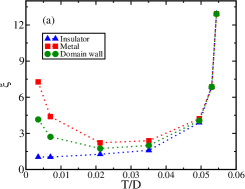
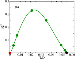
Figure 8: (a) Domain wall thickness as a function of temperature, displaying pronounced asymmetry at low temperature, where the thickness on the metallic side $\xi_{met}$ (red squares) becomes much larger than its insulating counterpart $\xi_{ins}$ (blue triangles). (b) The overall thickness $\xi=(\xi_{met}+\xi_{ins})/2$ (green circles in both panels) displays a square-root singularity at both $T=T_{c}$ (black dot) and the $T=0$ critical point (red dot).

What could be the mechanism leading to this strange behavior? An important clue is provided by comparing the behavior of the corresponding correlation length describing the domain wall profile, as shown in Fig. 8 (a). Here we observe that, while both $\xi_{met}$ and $\xi_{ins}$ diverge (and coincide) at $T\rightarrow T_{c}$, they behave very differently at $T\rightarrow 0$. Here $\xi_{met}$ diverges, but $\xi_{ins}$ saturates to a small value comparable to one lattice spacing. Physically, this result is easy to understand, keeping in mind the nature of the critical point at $U=U_{c2}$, which we approach as $T\rightarrow 0$ along the first order line. This critical point signals the instability of the metallic phase, where the characteristic energy scale of the quasi-particles vanishes and the free energy minimum corresponding to the metallic phase becomes unstable, leading to the divergence of $\xi_{met}$. In contrast, the insulating solution here remains stable, as its own instability arises only at a much smaller $U=U_{c1}\ll U_{c2}$, and the corresponding $\xi_{ins}$ thus remains short, as we find.

The resulting behavior of the overall domain wall thickness $\xi=(\xi_{met}+\xi_{ins})/2$ is even more clearly seen by plotting $\xi^{-2}$ as a function of temperature, which is seen to linearly vanish both at $T=T_{c}$ and $T=0$, as shown in Fig. 8 (b). While domain walls are generally expectedGoldenfeld (1992) to become thick at finite-temperature critical end-points ($T=T_{c}$), the presence of such behavior also at low temperatures deserves further comment and a proper physical interpretation. Within our DMFT formulation, it reflects the emergence of an additional critical point at $T=0$ and $U=U_{c2})$, corresponding to the divergence of the quasi-particle effective mass $m^{*}\sim(U_{c2}-U)^{-1}$, signaling a singular enhancement of the Sommerfeld specific-heat coefficient $\gamma=C/T\sim m^{*}$. This result, which is well-established within DMFT, reflects the approach to the Mott insulator characterized by large spin entropy at low temperatures. Physically, such neglect of significant inter-site spin correlations, as implied by the DMFT approximation, is expected to be justified in the limit of strong magnetic frustration, possibly in materials with triangular or Kagomé lattices.

IV Conclusions

In this paper we performed a detailed study of the structure and the dynamics of domains walls expected within the phase coexistence region around the Mott point. Our results, obtained within the DMFT approximation, suggest that such domain walls should display unusual dynamics, which is unlike that of a metal or that of an insulator, locally retaining strong inelastic (electron-electron) scattering down to very low temperatures. This curious behavior could be significant in systems where weak disorder and low dimensionality conspire to produce a substantial concentration of domain walls within the metal-insulator phase coexistence region. This behavior should be especially significant in systems where the domain walls remain sufficiently thick or fat over an appreciable temperature range, such that the domain wall matter covers a substantial volume (area) of a given sample. Our predictions could be even more directly tested by STM (scanning tunneling spectroscopy) experiments, which are able to locally probe transport properties at the center of a given domain walls, in even simpler geometries.

Our analysis also revealed that the mechanism favoring such thick domain walls is directly related to the degree of magnetic frustration characterizing the incipient Mott insulating state. In spatially inhomogeneous systems (e.g. due to lattice defects of other forms of structural disorder), one can imagine local regions with varying degrees of local magnetic frustration. The physical picture we put forward indicates direct consequences for the structure of the corresponding domain walls, with their local thickness being a direct measure of the local magnetic frustration. The work we presented in this paper is only the first step in the investigation of situations where the interplay of phase coexistence, strong correlations, and magnetic frustration should lead to exotic forms of dynamics of electrons, but more detailed investigations along these lines remain challenges for the future.

V acknowledgments

We thank Hanna Terleska for helpful discussions. We acknowledge support by CNPq (Brazil) through Grants No. 307041/2017-4 and No. 590093/2011-8, Capes (Brazil) through grant 0899/2018 (E.M.) and by the Texas Center for Superconductivity at the University of Houston (M.Y.S.V and J.H.M). Work in Florida (V. D. and T.-H. L.) was supported by the NSF Grant No. 1822258, and the National High Magnetic Field Laboratory through the NSF Cooperative Agreement No. 1157490 and the State of Florida.

appendix: Moving along the first order line

A close look at the results given in Fig. 5 reveals some details of the temperature dependence found, which deserve further clarification. It is clear that the DOS on the metallic side of the domain wall displays a noticeably non-monotonic $T$ dependence, which is generally not expected for a metallic phase at fixed $U$. However, it should be noted that we have here the simultaneous variation of both $T$ and $U$ when we follow the first-order transition line (FOTL) while reducing the temperature. This complicates the analysis, producing the non-monotonic behavior, as we see even more clearly in Fig. 9. Note, in particular, that the metallic DOS does not approach the non-interacting value (horizontal dotted line), even at low temperatures, in contrast to what one one finds by reducing $T$ at fixed $U$ (the so-called “pinning condition”, not shown).

To understand this behavior, we note that, at low temperatures, the metallic phase displays Fermi liquid behavior. In this case, all quantities become scaling functions of the reduced temperature $(T/T^{*}_{FL})$, where $T^{*}_{FL}\sim Z\sim(U_{c2}-U)$ is the Fermi liquid coherence scale and $Z$ is the quasiparticle weight.G. Moeller et al. (1999) Since, within DMFT, the FOTL also vanishes linearly with $(U_{c2}-U)$, the reduced temperature $(T/T^{*}_{FL})$ should remain finite even as $T\rightarrow 0$ along the FOTL line. This is the reason why the “pinning condition” is violated all along the FOTL. Indeed, within DMFT, the DOS is expected to approach its non-interacting value only at $T\ll T^{*}_{FL}$, a condition that is not satisfied anywhere along the FOTL. The remaining $T$ dependence we observe represents only sub-leading corrections, which are generally complicated and non-universal, consistent with the non-monotonic behavior we find.

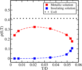
Figure 9: Evolution of the density of states (DOS) along the first-order transition line, shown for both the uniform metallic (top red curve) and the uniform insulating (bottom blue curve) solutions. For comparison we also show the non-interacting DOS value (horizontal dotted line), which is expected for the DOS in the metallic phase strictly at $T=0$.

References

- Mott (1990) N. F. Mott, Metal-Insulator transition (Taylor and Francis, London, 1990).
- Lederer et al. (1972) P. Lederer, H. Launois, J. P. Pouget, A. Casalot, and G. Villeneuve, Journal of Physics and Chemical of Solid 33, 1961 (1972).
- McWhan et al. (1973) D. B. McWhan, A. Menth, J. P. Remeika, W. F. Brinkman, and T. M. Rice, Phys. Rev. B. 7, 1920 (1973).
- Mazzaferro et al. (1980) J. Mazzaferro, H. Ceva, and B. Alascio, Phys. Rev. B. 22, 353 (1980).
- Limelette et al. (2003) P. Limelette, A. Georges, D. Jerome, P. Wzietek, P. Metcalf, and J. M. Honig, Science 302, 89 (2003).
- Qazilbash et al. (2007) M. M. Qazilbash, M. Brehm, B.-G. Chae, P.-C. Ho, G. O. Andreev, B.-J. Kim, S. J. Yun, A. Balatsky, M. B. Maple, F. Keilmann, et al., Science 318, 1750 (2007).
- Patrick A. Lee et al. (2006) Patrick A. Lee, Naoto Nagaosa, and Xiao-Gang Wen, Mod. Phys. 78, 17 (2006).
- Cai, P. et al. (2016) Cai, P., Ruan, W., Peng, Y., Ye. C, Li. X, Hao. Z, Zhou. X, Lee. D, and Wang. Y, Nature Physics 12, 1047 (2016).
- Hubbard (1957) J. Hubbard, Proc. R. Soc. (London) A 240, 539 (1957).
- Hubbard (1958) J. Hubbard, Proc. R. Soc. (London) A 243, 336 (1958).
- Brinkman and Rice (1970) W. F. Brinkman and T. M. Rice, Phys. Rev. B 2, 4302 (1970).
- A. Georges et al. (1996) A. Georges, G. Kotliar, W. Krauth, and M. J. Rozenberg, Rev. Mod. Phys. 68, 13 (1996).
- Kurosaki et al. (2005) Y. Kurosaki, Y. Shimizu, K. Miyagawa, K. Kanoda, and G. Saito, Phys. Rev. Lett. 95, 177001 (2005).
- Powell and McKenzie (2011) B. J. Powell and R. H. McKenzie, Reports on Progress in Physics 74, 056501 (2011).
- Dressel and Tomic (2020) M. Dressel and S. Tomic, Advances in Physics 69, 1 (2020).
- Vollhardt (2020) D. Vollhardt, JPS Conf. Proc. 30, 011001 (2020).
- Furukawa et al. (2015) T. Furukawa, K. Miyagawa, H. Taniguchi, R. Kato, and K. Kanoda, Nat. Phys. 11, 221 (2015).
- H. Terletska et al. (2011) H. Terletska, J. Vucicević, D. Tanasković, and V. Dobrosavljević, Phys. Rev. Lett 84, 125120 (2011).
- Vučičević et al. (2013) J. Vučičević, H. Terletska, D. Tanasković, and V. Dobrosavljević, Phys. Rev. B 88, 75143 (2013).
- Pustogow et al. (2018) A. Pustogow, M. Bories, A. Löhle, R. Rösslhuber, E. Zhukova, B. Gorshunov, S. Tomić, J. A. Schlueter, R. Hübner, T. Hiramatsu, et al., Nat. Mater. 17, 773 (2018).
- Pustogow et al. (2021) A. Pustogow, R. Rösslhuber, Y. Tan, E. Uykur, A. Böhme, M. Wenzel, Y. Saito, A. Löhle, R. Hübner, A. Kawamoto, et al., npj Quantum Materials 6, 1 (2021).
- Pruschke et al. (1995) T. Pruschke, M. Jarrell, and J. K. Freericks, Adv. Phys. 44, 187 (1995).
- Kotliar and Vollhardt (2004) G. Kotliar and D. Vollhardt, Physics Today 57, 53 (2004).
- M. Y. Suárez-Villagrán et al. (2020) M. Y. Suárez-Villagrán, N. Mitsakos, Tsung-Han Lee, V. Dobrosavljević, J. H. Miller Jr., and E. Miranda, Phys, Rev B 101, 235112 (2020).
- Miranda and Dobrosavljević (2005) E. Miranda and V. Dobrosavljević, Rep. Prog. Phys. 68, 2337 (2005).
- Tanasković et al. (2003) D. Tanasković, V. Dobrosavljević, E. Abrahams, and G. Kotliar, Phys. Rev. Lett. 91, 066603 (2003).
- Dobrosavljević et al. (2003) V. Dobrosavljević, D. Tanasković, and A. A. Pastor, Phys. Rev. Lett. 90, 016402 (2003).
- M. C. O. Aguiar et al. (2004) M. C. O. Aguiar, E. Miranda, V. Dobrosavljević, E. Abrahams, and G. Kotliar, Europhys. Lett. 67, 226 (2004).
- Aguiar et al. (2005) M. C. O. Aguiar, V. Dobrosavljević, E. Abrahams, and G. Kotliar, Phys. Rev. B 71, 205115 (2005).
- Aguiar et al. (2009) M. C. O. Aguiar, V. Dobrosavljević, E. Abrahams, and G. Kotliar, Phys. Rev. Lett. 102, 156402 (2009).
- Andrade et al. (2009) E. C. Andrade, E. Miranda, and V. Dobrosavljević, Phys. Rev. Lett. 102, 206403 (2009).
- Andrade et al. (2010) E. C. Andrade, E. Miranda, and V. Dobrosavljević, Phys. Rev. Lett. 104, 236401 (2010).
- Papanikolaou et al. (2008) S. Papanikolaou, R. M. Fernandes, E. Fradkin, P. W. Phillips, J. Schmalian, and R. Sknepnek, Phys. Rev. Lett. 100, 026408 (2008).
- Lee and Yee (2017) J. Lee and C.-H. Yee, Phys. Rev. B 95, 205126 (2017).
- Adler et al. (2018) R. Adler, C.-J. Kang, C.-H. Yee, and G. Kotliar, Reports on Progress in Physics 82, 012504 (2018).
- Goldenfeld (1992) N. Goldenfeld, Lectures on phase transitions and critical phenomena, Frontiers in Physics, 85 (Westview Press, 1992), illustrated edition ed., ISBN 9780201554090,0201554097.
- Helmes et al. (2008) R. W. Helmes, T. A. Costi, and A. Rosch, Phys. Rev. Lett. 101, 066802 (2008).
- Potthoff and Nolting (1999) M. Potthoff and W. Nolting, Phys. Rev. B 59, 2549 (1999).
- Metzner and Vollhardt (1989) W. Metzner and D. Vollhardt, Phys. Rev. Lett. 62, 324 (1989).
- A. Georges and G. Kotliar (1992) A. Georges and G. Kotliar, Phys. Rev. B 45, 6479 (1992).
- G. Moeller et al. (1999) G. Moeller, V. Dobrosavljević, and A.E. Ruckenstein, Phys. Rev. B 59, 6846 (1999).
- Dobrosavljević and Kotliar (1997) V. Dobrosavljević and G. Kotliar, Phys. Rev. Lett. 78, 3943 (1997).
- Dobrosavljević and Kotliar (1998) V. Dobrosavljević and G. Kotliar, Phil. Trans. R. Soc. Lond. A 356, 1 (1998).
- E. Miranda and V. Dobrosavljević (2012) E. Miranda and V. Dobrosavljević, in Conductor-Insulator Quantum Phase Transitions, edited by Vladimir Dobrosavljević, Nandini Trivedi, and James M. Valles, Jr. (Oxford University Press, Oxford, 2012), pp. 161–243.
- H. Kajueter and G. Kotliar (1996) H. Kajueter and G. Kotliar, Phys. Rev. Lett. 77, 131 (1996).
- Zhang et al. (1993) X. Y. Zhang, M. J. Rozenberg, and G. Kotliar, Phys. Rev. Lett. 70, 1666 (1993).
- H. J. Vidberg and J. W. Serene (1977) H. J. Vidberg and J. W. Serene, Journal of Low Temperature Physics 29, 179 (1977).
- Castellani et al. (1979) C. Castellani, C. D. Castro, D. Feinberg, and J. Ranninger, Phys. Rev. Lett. 43, 1957 (1979).
- Rozenberg et al. (1999) M. J. Rozenberg, R. Chitra, and G. Kotliar, Phys. Rev. Lett. 83, 3498 (1999).
- Kotliar et al. (2000) G. Kotliar, E. Lange, and M. J. Rozenberg, Phys. Rev. Lett. 84, 5180 (2000).
- Abdel-Jawad et al. (2015) M. Abdel-Jawad, R. Kato, I. Watanabe, N. Tajima, and Y. Ishii, Phys. Rev. Lett. 114, 106401 (2015).