Moiré effects in graphene–hBN heterostructures

Abstract

Encapsulating graphene in hexagonal Boron Nitride has several advantages: the highest mobilities reported to date are achieved in this way, and precise nanostructuring of graphene becomes feasible through the protective hBN layers. Nevertheless, subtle effects may arise due to the differing lattice constants of graphene and hBN, and due to the twist angle between the graphene and hBN lattices. Here, we use a recently developed model which allows us to perform band structure and magnetotransport calculations of such structures, and show that with a proper account of the moiré physics an excellent agreement with experiments can be achieved, even for complicated structures such as disordered graphene, or antidot lattices on a monolayer hBN with a relative twist angle. Calculations of this kind are essential to a quantitative modeling of twistronic devices.

I Introduction

Graphene, the first successfully isolated two-dimensional material, has opened a new hot research areaGraphene-1 ; Graphene-2 . Due to the linear bands crossing the Fermi level, low-energy carriers in graphene behave like massless, relativistic Dirac fermions, allowing predictions from quantum electrodynamics to be tested in a solid-state system. The high Fermi velocityhighVF , Dirac-cone band structureGraphene-1 and ultra-strong mechanical propertiesmechanical make graphene a promising material for next-generation electronic nanodevices and high-speed switching devices. However, the intrinsic zero energy gap of graphene has hampered its applications in modern electronics. In a practical nanoelectronic device semiconducting graphene is necessary.

A sizable band gap opening around the Fermi level in a graphene antidot lattice (GAL, a regular arrangement of antidots in a graphene lattice) has been predicted by several theoretical studiesGAL-PRL ; GAL-theory-2 ; GAL-theory-3 ; GAL-theory-4 ; GAL-theory-5 , and was recently realized in an experimentNat-tech-2019 . The band gap in GAL can be tuned by the size, shape, and symmetry of both the antidot and the superlattice cellGAL-PRL ; GAL-theory-2 ; GAL-theory-3 ; GAL-theory-4 ; GAL-theory-5 . The tunable band gap can be used to design quantum wells and channels for electronic devicesGAL-PRL ; GAL-theory-2 ; GAL-theory-3 ; GAL-theory-4 ; GAL-theory-5 . Interestingly, transport under magnetic fields in an antidot lattice is predicted to show Hofstadter butterfly features arising from the competition between the antidot lattice periodicity and the magnetic lengthGAL-magnetic .

Recently, heterostructures consisting of graphene and hexagonal boron nitride (G/hBN) have drawn intense attentionNat-tech-2019 ; G-hBN-PRL-relax ; G-hBN-PRL-relax-2 ; G-hBN-Hofstadter-PRL ; G-hBN-Hofstadter ; G-hBN-Hofstadter-sci ; G-hBN-Cloning-Dirac ; G-hBN-NC-band-gap ; G-hBN-PRL-gap ; G-hBN-FQH-sci ; G-hBN-review ; G-hBN-review-2 ; G-hBN-natphys . The lattice mismatch between graphene and hBN causes moiré patterns with long wavelengths to emerge when graphene and hBN lattices are exactly aligned or twisted relatively by a small angleG-hBN-PRL-relax ; G-hBN-PRL-relax-2 . Experiments have revealed many exciting phenomena, such as the Hofstadter butterflyNat-tech-2019 ; G-hBN-Hofstadter ; G-hBN-Hofstadter-sci ; G-hBN-Cloning-Dirac ; G-hBN-review ; G-hBN-review-2 (now arising from the competition between the lattice mismatch induced moiré length and the magnetic length), or the fractional quantum Hall effectG-hBN-FQH-sci ; G-hBN-review ; G-hBN-review-2 . However, the twist-angle dependence of the properties of antidot lattices defined on G/hBN heterostructures has not yet been the subject of a systematical experimental or theoretical study. Another system where moiré effects show up dramatically is twisted bilayer graphene, where unconventional superconductivity or correlated insulator behavior may occur at certain twist angles between the monolayers BiGr-Nature1 ; BiGr-Nature2 .

In this paper we consider two examples of recent experimental interest where the relative angle between graphene and hBN plays an important roleNat-tech-2019 ; Expdisorder : (i) disordered graphene, and (ii) antidot lattices. We first summarize our most important physical findings, and discuss the technical details in subsequent paragraphs. By using an effective lattice model, we first calculate the electronic structure and conductance of G/hBN with and without a relaxation of the graphene and hBN monolayers comprising the system. Our results show that without relaxation the band structure is particle-hole symmetric, in disagreement with experimental data, while the fully relaxed graphene shows, correctly, a particle-hole asymmetry emphasizing the importance of lattice relaxation of G/hBN. Next, we compute the conductance in the presence of a magnetic field perpendicular to the graphene sheet. The computed magnetoconductance shows a moiré potential induced secondary Dirac point which clones the Landau fan of the primary Dirac point. The Hofstadter butterfly features are also observed in our numerical results. The computed results are in excellent agreement with experimental dataNat-tech-2019 ; G-hBN-Hofstadter ; G-hBN-Hofstadter-sci ; G-hBN-Cloning-Dirac . Based on an Anderson model, we next investigate how disorder affects the electronic structure and conductance of G/hBN. We find that even though disorder can lift the degeneracy of the bands at high symmetry points, the main features of the band structure are similar to the clean case. While the magnitude of the conductance with disorder is reduced to almost a half of the one without disorder, the magnetoconductance stays unchanged. Finally, we systematically study the electronic structure and transport behavior of antidot lattice on twisted G/hBN. A major theoretical finding is that the secondary Dirac point will disappear once the distance between antidot edges ("the neck width", denoted by $d_{n}$ and see Appendix F) is smaller than the moiré wave length, a feature seen in experiments Nat-tech-2019 .

II The model

Our effective tight-binding model is proposed in Ref.model-PRB and we follow the procedures outlined there (Appendix A summarizes the details pertinent to this work). Carbon atoms can be removed from the antidot regions by removing the associated rows and columns from the system Hamiltonian. Any dangling $\sigma$ bonds for a carbon atom with only two neighboring carbon atoms are assumed to be passivated with Hydrogen atoms so that the $\pi$ bands are unaffected. Transport quantities are calculated using recursive Green’s function techniques, following Ref.greenfunction . The zero-temperature conductance is given by the Landauer formula $G=\frac{2e^{2}}{h}T$, where $T$ is transmission coefficient. A finite magnetic field $B$ perpendicular to the graphene plane is modeled by associating a Peierls phase to the hopping amplitude $t\rightarrow te^{i\varphi_{ij}}$, where $\varphi_{ij}=(e/\hbar)\int_{r_{i}}^{r_{j}}\mathbf{A}\cdot d\mathbf{r}$. Here $\mathbf{A}$ is the vector potential and $r_{i}$ is the position of atom $i$. We choose the Landau gauge $\mathbf{A}=(-By,0,0)$, and the Peierls phase becomes $\varphi_{ij}=\frac{eB}{\hbar}(x_{j}-x_{i})(\frac{y_{i}+y_{j}}{2})$. In the leads the magnetic field is set to zero.

Microscopic theoretical investigations on the G/hBN system are made cumbersome by the size of the unit cell, which for small relative rotations contains thousands of atoms making first-principles calculations very expensive. Effective continuum modelscontinmodel or several tight-binding modelsG-hBN-Hofstadter-PRL ; empirical with empirical parameters controlling the interlayer interaction between graphene and hBN have been applied to calculate the electronic properties of G/hBN. However, the effective continuum model cannot be used to simulate the transport for realistic experimental conditions, while results for the tight-binding models with empirical parameters must be carefully scrutinized to ascertain their reliability. For a large device transport simulation Chen et al.scalerpotential applied a scaled graphene lattice with a triangular periodic scalar moiré potential, and successfully reproduced the main features of the secondary Dirac point. However, as we show below, this simple moiré potential does not lead to particle-hole asymmetry. In our effective lattice model, the Hamiltonian terms at any local part of a twisted and relaxed G/hBN only depend on the local relative shift and relaxation-induced strain and can be derived from a transparent set of parameters calculated by density functional theory. Moreover, our effective lattice model can be used to calculate the electronic structure of G/hBN with any twist angle, and does not require a recalculation of the parameters for a new twist angle.

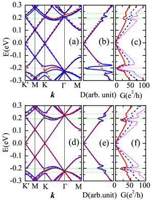
Figure 1: The calculated electronic structure of G/hBN with twist angle 1.0047^∘. (a), (b) and (c) are calculated with relaxation while (d), (e), and (f) are without lattice relaxation. (a) and (d) show the band structures; (b) and (e) are the densities of states; (c) and (f) give the conductance without magnetic field. In the band structure and DOS, the red dashed lines denote the graphene monolayer for comparison. In the conductances (c) and (f), the red solid, blue dashed, and magenta dot lines are calculated for device sizes 200 nm$\times$ 200 nm, 300 nm$\times$300 nm, and 400 nm$\times$400 nm, respectively. The thin dashed green lines indicate the minima in DOS.

We next calculate the band structure and conductance for the twist angle $\theta$=1.0047^∘ with and without lattice relaxation; the results are reported in Fig. 1. The band structure (Fig.1(a)) and density of states (DOS) (Fig.1(b)) of fully relaxed G/hBN show a particle-hole asymmetry which is consistent with the experimentsNat-tech-2019 ; G-hBN-Hofstadter ; G-hBN-Hofstadter-sci ; G-hBN-Cloning-Dirac ; G-hBN-PRL-gap ; G-hBN-FQH-sci ; G-hBN-review ; G-hBN-review-2 . To emphasize the importance of full relaxation, we plot in Fig. 1(d) the band structure of graphene with a scalar moiré potentialscalerpotential : the band degeneracy at high symmetry points is lifted and one finds secondary Dirac points at $\pm$0.225eV. However, in this case the DOS around the two secondary Dirac points are equal and obey particle-hole symmetry (Fig.1(e)), in contrast to experiment, and Fig. 1(a) and 1(b). The reason for the difference is that a fully relaxed graphene lattice has, in addition to a modified on-site energy, also a modified hopping between neighboring C atoms.

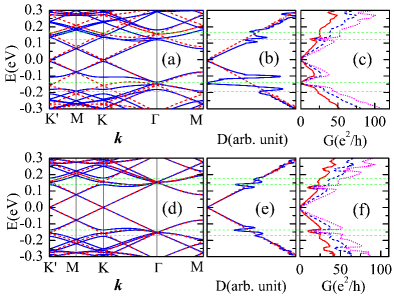
Figure B1: The calculated electronic structure of G/hBN with twist angle 0.0^∘. (a), (b) and (c) are calculated with relaxation while (d), (e), and (f) are without lattice relaxation. (a) and (d) display the band structures; (b) and (e) are the densities of states; (c) and (f) are the conductance without magnetic field. In the band structure and DOS, the red dashed lines denote the graphene monolayer results. In the conductance (c) and (f), the red solid, blue dashed, and magenta dot lines are calculated for device sizes 200nm$\times$200nm, 300nm$\times$300nm, and 400nm$\times$400nm, repectively.

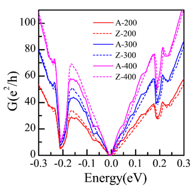
Figure C1: The conductance of G/h-BN for devices with zigzag edge (Z) and armchair edge (A), with twist angle 1.0047^∘. Solid lines denote zigzag edges with while dashed lines are for armchair edges. The device sizes are 200 nm $\times$ 200 nm, 300 nm$\times$300 nm, and 400nm$\times$400nm, respectively.

Appendices B and C report the band structure and conductance for additional twist angles and edge orientations. The two main conclusions are: (i) the secondary Dirac points shift to larger energies as the twist angle increases, because the interaction between graphene and hBN decreases as the twist angle increases (see Fig. B1-B3), and (ii) the calculated conductance does not significantly depend on whether the edges of the simulated device are in the armchair or zigzag directions (see Fig. C1). In subsequent calculations we consider a device with zigzag edges.

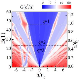
Figure 2: Longitudinal magnetoconductance $G(B,n)$ as a function of magnetic field and electron density. Here $n$ is electron density, $n_{0}=1/S$ is the electron density per each Bloch band, where $S$ is the area of supercell. Right vertical axis is scaled by $\phi/\phi_{0}$ where $\phi$ is the flux through one moiré unit cell and $\phi_{0}=h/e$ is the flux quantum. Dashed black lines show $q$=1, 2, and 3, where the Landau levels intersect.

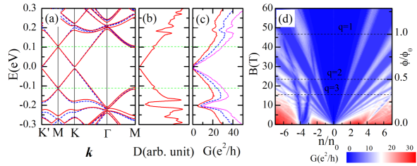
Figure 3: The electronic structure and conductance of G/hBN with disorder with twist angle 1.0047^∘. (a) Red solid line: band structure with disorder. Dashed blue line: band structure for pristine sample. (b) Density of states. (c) Zero-field conductance. Red, blue, and magenta lines refer to device sizes of 200 nm $\times$ 200 nm, 300nm $\times$ 300 nm and 400nm $\times$ 400nm, respectively. (d) Magnetoconductance for a disordered sample.

We next carry out magnetotransport simulations using the effective lattice model for a 300 nm$\times$300 nm device ($\simeq 10^{7}$ atoms). Our results are shown in Fig. 2 (some finer details in $G$, not visible in Fig. 2, are discussed in Appendix D). Both the primary ($n/n_{0}=0$) and the secondary Dirac points ($n/n_{0}=\pm 4$) break into sequences of Landau levels upon application of a magnetic field, forming the so called Hofstadter butterfly spectrum. The high conductance areas (red, white) separate the gapped Landau levels (blue). As mentioned above, the moiré superlattice potential breaks the partical-hole symmetry, as also seen in transport experiments Nat-tech-2019 ; G-hBN-Hofstadter ; G-hBN-Hofstadter-sci ; G-hBN-Cloning-Dirac ; G-hBN-PRL-gap ; G-hBN-FQH-sci ; G-hBN-review ; G-hBN-review-2 . As the magnetic field increases, the Landau levels will intersect when $\frac{\phi}{\phi_{0}}=\frac{1}{q}$, where $q$ is an integer, indicated in Fig. 2 with black dashed lines. The intersection of the primary and secondary Landau levels leads to a closing of the magnetic band gap, and a resulting high conductivity, seen as bright spots in Fig. 2. Results for other twist angles, showing the same general trends, are given in Appendix B.

III Effects due to disorder

Disorder is ubiquitous to all graphene samples, even for those synthesized with state-of-the-art technologiesdisorder-1 . The properties of nanoribbons are known to be strongly affected by disorder disorderribbon , and recent studies suggest that the electronic and transport properties of graphene antidot lattice may also be strongly perturbed by relatively modest disorderdisorder-2 ; disorder-3 ; disorder-4 ; disorder-5 ; disorder-6 . An exploration of the effect of disorder on G/hBN is thus called for. Here, we introduce disorder as a site-diagonal random potential with matrix element $H_{ij}=\delta_{ij}v_{i}$, where $v_{i}$ are independent, uniformly distributed random variables in the range of [-$V_{0}$,$V_{0}$] (where $V_{0}$ is set to 0.5eV larger than the onsite energy $\varepsilon_{i}$, maximum 0.14eV), and have zero mean and unit variance. Other details on the disorder model are provided in Appendix E. One would expect that disorder breaks certain symmetries with concomitant modifications in the band structure. Here, our simulations show that disorder leads to band degeneracy lifting at high symmetry points, especially it opens a band gap at the M point (Fig. 3(a)). The band gap opening leads to a kink in DOS (indicated by horizontal green lines in Fig. 3 (b)). Even though the DOS is modified by disorder, the generic features in conductance stay qualitatively unchanged, except for an overall reduction of $\simeq 50\%$ in magnitude (compare Fig. 1(c) and 3(c)). In particular, the features in the conductivity at the secondary Dirac points still remain. Overall, we conclude that the transport properties of G/hBN at $B=0$ are very robust against disorder.

To investigate whether the robustness persists for finite magnetic fields, we next calculate the magnetotransport properties of disordered G/hBN; the results are shown in Fig. 3(d). One observes that the main features of the magnetoconductivity are essentially the same as those without disorder, shown in Fig. 2. The main differences are the overall reduction of magnetoconductiviy, as already discussed above, and that many fine features are washed out by disorder, and thus the results for the disordered system appear significantly more regular than those for the pristine system. The conclusion is that the magnetotransport in G/hBN is indeed robust with respect to disorder, and its salient features should survive even a nonideal fabrication process.

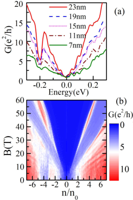
Figure 4: (a) Zero-field conductances for antidot lattices with different neck widths ($d_{n}=7$, $11$, $15$, $19$, $23$ nm). The secondary feature at $E\simeq-0.2$ eV disappears if the neck width $d_{n}$ is smaller than moiré length $\lambda=10.1$ nm for the twist angle=1.0047^∘. (b) Landau fan diagram with for neck width $d_{n}=15$ nm.

IV Antidot lattices

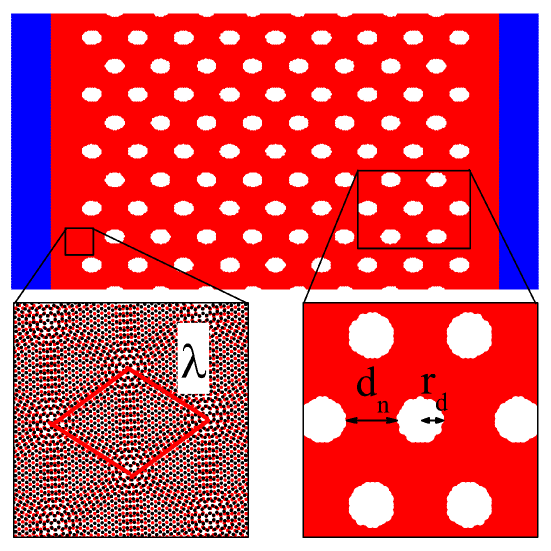
Figure F1: Schematic of the device. Blue areas are the left and the right lead, and red area is the scattering region. The enlarged figures (bottom panels) show the moiré wave length $\lambda$, the neck width $d_{n}$, and the radius $r_{d}$ of the antidot. The lattice constant of the antidot lattice is $a_{antidot}=d_{n}+2r_{d}$. In our calculations we set $a_{antidot}=35$ nm, and vary the antidot’s radius to generate different neck widths.

The band structure of graphene antidot lattices (GAL) may differ qualitatively from that of graphene, as witnessed by the observation of a band gap in recent experimentsNat-tech-2019 . We next describe how the techniques developed in this work can yield additional important information of transport in a GAL on a (twisted) hBN substrate. In addition to the magnetic length, there are now two (at least) other competing other length scales: the moiré length $\lambda$, which is maximally 14.4 nmmodel-PRB , and the length scale(s) characterizing the GAL. A schematic geometry of the GAL system is shown in Fig. F1. We consider triangular antidot lattices, because they are known to lead to gapped systemsGAL-theory-4 Our numerical results reveal an important relationship between $\lambda$ and $d_{n}$. The secondary Dirac point features in conductance are observed only when $d_{n}>\lambda$, while they vanish if $d_{n}<\lambda$ as shown in Fig. 4(a). This finding explains an important detail in the recent experimentsNat-tech-2019 . Namely, pristine graphene encapsulated in hBN shows a primary Landau fan and two cloned fans corresponding to moiré periods of 10.2nm and 17.2nm. The second moiré length is larger than the longest possible moiré length in single layer graphene on hBN. Recent experimental and theoretical studies show that the second moiré pattern is due to the simultaneous effects of top and bottom hBN supermoire-1 ; supermoire-2 ; supermoire-3 ; supermoire-4 . However, after fabrication of the GAL the second peak related to the 17.2 nm moiré wavelength is lost. As the neck length in the fabricated GALs is 12-15nm, and thereby smaller than the second moiré wavelength 17.2 nm, one does not expect to see Landau fans related to this length scale, which indeed is the case in the experiment. In Fig. 4(b) we show the Landau fan diagram of G/hBN with an antidot lattice whose $d_{n}=15$ nm. Compared to the results shown in Fig. 2, there is a reduction in both the magnitude of magnetoconductance, and the number of Landau levels. Importantly, the secondary Dirac point survives, just as in experimentsNat-tech-2019 .

V Conclusion

In summary, we have performed a systematic examination of the consequences of the lattice mismatch and relative orientation between graphene and hBN, and show that several experimental observations find a common explanation rooted in the interplay of the moiré length, and other relevant length scales. The method described in this work can be extended to many other systems of current interest, including twistronic devices.

VI Acknowledgments

The work was supported by the Jiangsu Province Science Foundation for Youth (Grant No. BK20170821), National Science Foundation of China for Youth (Grant No. 11804160) and National Natural Science Foundation of China (Grant No. 11974312). The Center for Nanostructured Graphene (CNG) is sponsored by the Danish National Research Foundation, Project No. DNRF103.

Appendix A Appendix A: Effective lattice model

The effective lattice Hamiltonian for graphene and hexagonal boron nitride (G/hBN) reads

$$H=\sum_{i}(h_{Ai}c_{Ai}^{\dagger}c_{Ai}+h_{Bi}c_{Bi}^{\dagger}c_{Bi})-\sum_{<i,j>}t_{ij}(c_{Ai}^{\dagger}c_{Bj}+c_{Bj}^{\dagger}c_{Ai}),$$ (1)

where $c_{mi}^{\dagger}$ is the creation and $c_{mi}$ is the annihilation operator of $p_{z}$ state in sublattice $m$ and unit cell $i$, $h_{mi}$ and $t_{ij}$ represent on-site energies and hopping terms. Here we set $h_{0}=(h_{A}+h_{B})/2$ and $h_{z}=(h_{A}-h_{B})/2$. The hopping terms along the three nearest-neighbor vectors $\delta_{n}$ with $n=1-3$ (see Fig.1 in Ref.model-PRB ) are represented by $-t_{n}$.

A.1 First step: hopping terms and on-site energies at point $\mathbf{r}$ for rigid G/hBN

As the analysis in Ref.model-PRB shows, in a large moiré superlattice the local lattice structure is similar to that of a shifted G/hBN bilayer where both layers have the same orientation and the same lattice constant as monolayer graphene (see Fig. 1 in Ref.model-PRB ). First-principles calculations show that the electronic structure of the shifted G/hBN is periodic in the shift vector $\mathbf{d}$ with the lattice vectors of graphene determining the period. Thus, for every shift vector $\mathbf{d}$, we can derive the hopping parameters $t_{n}$ and on-site energies $h_{0}$ and $h_{z}$ by fitting the band structure from first-principles calculations. The resluts show that $t_{n}$, $h_{0}$ and $h_{z}$ are also periodic in the shift vector $\mathbf{d}$. Since the $t_{n}$, $h_{0}$ and $h_{z}$ in effective lattice model are periodic in vector $\mathbf{d}$, they can be expanded in Fourier series, such as

$$t_{n}(\mathbf{d}) = \sum_{\mathbf{G}}\widetilde{t}_{n}(\mathbf{G})\cos[\mathbf{G}\cdot\mathbf{d}+\phi_{n}(\mathbf{G})]$$ (2)

$$h_{0}(\mathbf{d}) = \sum_{\mathbf{G}}\widetilde{h}_{0}(\mathbf{G})\cos[\mathbf{G}\cdot\mathbf{d}+\phi_{0}(\mathbf{G})]$$ (3)

$$h_{z}(\mathbf{d}) = \sum_{\mathbf{G}}\widetilde{h}_{z}(\mathbf{G})\cos[\mathbf{G}\cdot\mathbf{d}+\phi_{z}(\mathbf{G})]$$ (4)

where $\mathbf{G}$ are the reciprocal lattice vectors of graphene and 10 shortest vectors including the origin are used in the expansion. $\overset{\sim}{t}_{n}(\mathbf{G})$ ($\overset{\sim}{h}_{0}(\mathbf{G})$, $\overset{\sim}{h}_{z}(\mathbf{G})$) and $\phi_{n}(\mathbf{G})$ ($\phi_{0}(\mathbf{G})$, $\phi_{z}(\mathbf{G})$)are the amplitudes and corresponding phase. The expansion parameters for $t_{n}$, $h_{0}$ and $h_{z}$ are listed in Table A1.

$G$	$\widetilde{t}_{1}$	$\phi_{1}(^{\circ})$	$\widetilde{t}_{2}$	$\phi_{2}(^{\circ})$	$\widetilde{t}_{3}$	$\phi_{3}(^{\circ})$	$\widetilde{h}_{0}$	$\phi_{0}(^{\circ})$	$\widetilde{h}_{z}$	$\phi_{z}(^{\circ})$
(0,0)	2540.23	0.00	2540.23	0.00	2540.23	0.00	0.00	0.00	2.13	0.00
(1,0)	16.78	132.90	10.45	-151.18	16.78	132.90	25.12	-80.83	12.47	179.52
(-1,1)	16.78	132.90	16.78	132.90	10.45	-151.18	25.12	-80.83	12.47	179.52
(0,-1)	10.45	-151.18	16.78	132.90	16.78	132.90	25.12	-80.83	12.47	179.52
(1,1)	2.55	-17.69	2.55	17.69	4.05	0.00	2.86	-180.00	1.29	0.00
(-2,1)	4.05	0.00	2.55	-17.69	2.55	17.69	2.86	-180.00	1.29	0.00
(1,-2)	2.55	17.69	4.05	0.00	2.55	-17.69	2.86	-180.00	1.29	0.00
(2,0)	2.20	-103.20	0.98	60.31	2.20	-103.20	1.95	51.47	1.04	-52.14
(-2,2)	2.20	-103.20	2.20	-103.20	0.98	-60.31	1.95	51.47	1.04	-52.14
(0,-2)	0.98	-60.31	2.20	-103.20	2.20	-103.20	1.95	51.47	1.04	-52.14

Table A1: The parameter of the Fourier expansion of $t_{n}(n=1-3)$, $h_{0}$, and $h_{z}$. $\widetilde{t}_{n}$, $\widetilde{h}_{0}$, and $\widetilde{h}_{z}$ are the expansion amplitudes and are in the unit of meV. $\phi_{n}$, $\phi_{0}$, and $\phi_{z}$ are the corresponding expansion angles. $\mathbf{G}=n_{1}\mathbf{b}_{1}+n_{2}\mathbf{b}_{2}$ are the used reciprocal lattice. $\mathbf{b}_{1}$ and $\mathbf{b}_{2}$ are the reciprocal vector for graphene. The data is adapted with permission from Ref.model-PRB .

With the obtained parameters, we can get the hopping terms and on-site energies around a point r for effective lattice model because the local lattice structure of moiré superlattice can be approximated as a shifted bilayer with $\mathbf{d}(\mathbf{r})$. For a rigid superlattices, $\mathbf{d}(\mathbf{r})=(S^{-1}-I)\mathbf{r}$, where $I$ is unit matrix and $S=\frac{\begin{array}[]{c}1\end{array}}{\begin{array}[]{c}1+\epsilon\end{array}}\left(\begin{array}[]{cc}\cos\theta&-\sin\theta\\ \sin\theta&\cos\theta\end{array}\right)$, $\theta$ is twist angle between graphene and hexagonal boron nitride (hBN), $\epsilon=(a_{G}-a_{hBN})/a_{hBN}$. Here, $a_{G}$ and $a_{hBN}$ are the lattice constant for graphene and hBN, respectively.

A.2 Second step: relaxation of G/hBN

Due to the energy gain from the larger domains of energetically favorable stacking configurations (AB stacking), the rigid G/hBN bilayer undergoes spontaneous relaxation. The full lattice relaxation can be calculated by solving three equations self-consistentlymodel-PRB as we show below. We define $\mathbf{u}^{1}(\mathbf{r})$ and $\mathbf{u}^{2}(\mathbf{r})$ (see Fig. 1 in Refmodel-PRB , and Fig. 3 in BilayerG ) are the displacement vector for top graphene layer and bottom hBN layer, respectively. The total energy ($E_{tot}$) of bilayer supercell is the summation of the elastic energy ($E_{el}$) and interlayer interaction energy $E_{int}$ and also is a functional of the displacement vector $\mathbf{u}^{j}(\mathbf{r})$. The elastic energy ($E_{el}$) is given bymodel-PRB ; BilayerG :

$$E_{el}=\overset{2}{\sum_{\mathbf{j=1}}}\int d\mathbf{r}\left\{\frac{\lambda_{j}+\mu_{j}}{2}\left(\mathbf{\frac{\partial u_{x}^{j}}{\partial x}+\frac{\partial u_{y}^{j}}{\partial y}}\right)^{2}+\frac{\mu_{j}}{2}\left[\left(\mathbf{\frac{\partial u_{x}^{j}}{\partial x}-\frac{\partial u_{y}^{j}}{\partial y}}\right)^{2}+\left(\mathbf{\frac{\partial u_{y}^{j}}{\partial x}+\frac{\partial u_{x}^{j}}{\partial y}}\right)^{2}\right]\right\}$$ (5)

where $\lambda_{1}=3.653eV/\mathring{A}^{2}$, $\mu_{1}=9.125eV/\mathring{A}^{2}$; $\lambda_{2}=1.779eV/\mathring{A}^{2}$, $\mu_{2}=7.939eV/\mathring{A}^{2}$ are the elastic Lamé factors for graphene and hBN, respectively.

The interlayer interaction energy $E_{int}$ can be written asmodel-PRB ; BilayerG :

$$E_{int}=\int V[\mathbf{d}(\mathbf{r})]d\mathbf{r}$$ (6)

where $V[\mathbf{d}(\mathbf{r})]=\widetilde{V}\underset{k=1}{\overset{3}{\sum}}\cos(\mathbf{G}_{k}\cdot\mathbf{d}(\mathbf{r})+\phi_{V})$. For $\mathbf{G}_{k}$ we have $\mathbf{G}_{1}=\mathbf{b}_{1}$, $\mathbf{G}_{2}=-\mathbf{b}_{1}+\mathbf{b}_{2}$, $\mathbf{G}_{3}=-\mathbf{b}_{2}$. $\widetilde{V}$ takes 4.38 while $\phi_{V}=-50.26{{}^{\circ}}$.

The minimization of total energy ($E_{tot}$) as a functional of $\mathbf{u}^{j}(\mathbf{r})$ leads to a set of Euler-Lagrange equations by using a similar procedure as in Ref.model-PRB ; BilayerG :

$$\left(\begin{array}[]{c}\widetilde{u}_{x}^{j}(\mathbf{q})\\ \widetilde{u}_{y}^{j}(\mathbf{q})\end{array}\right)=(-1)^{j}\left(\begin{array}[]{cc}(\lambda_{j}+2\mu_{j})q_{x}^{2}+\mu_{j}q_{y}^{2}&(\lambda_{j}+\mu_{j})q_{x}q_{y}\\ (\lambda_{j}+\mu_{j})q_{x}q_{y}&(\lambda_{j}+2\mu_{j})q_{y}^{2}+\mu_{j}q_{x}^{2}\end{array}\right)^{-1}\left(\begin{array}[]{c}f_{x}^{j}(\mathbf{q})\\ f_{y}^{j}(\mathbf{q})\end{array}\right)$$ (7)

where $\mathbf{q}$ takes each $\mathbf{G}_{s}$, $\mathbf{G}_{s}$ are the reciprocal lattice vectors of the supercell and 60 shortest nonzero ones have been used. $j=1,2$ represent top graphene layer ($j=1$) and bottom hBN layer ($j=2$). The Fourier components $\widetilde{\mathbf{u}}^{j}(\mathbf{G}_{s})$, and $\mathbf{f}^{j}(\mathbf{G}_{s})$ are defined as

$$\mathbf{u}^{j}(\mathbf{r}) = \sum_{\mathbf{G}_{s}}\widetilde{\mathbf{u}}^{j}(\mathbf{G}_{s})e^{i\mathbf{G}_{s}\cdot\mathbf{r}}$$ (8)

$$\frac{\partial V(\mathbf{d})}{\partial\mathbf{d}} = -\widetilde{V}\underset{k=1}{\overset{3}{\sum}}\sin(\mathbf{G}_{k}\cdot\mathbf{((S^{-1}-I)\mathbf{r+u}^{\mathbf{1}}\mathbf{(r)-u}^{2}\mathbf{(r)})}+\phi_{V})\mathbf{G}_{k}=\sum_{\mathbf{G}_{s}}\mathbf{f}^{j}(\mathbf{G}_{s})e^{i\mathbf{G}_{s}\cdot\mathbf{r}}$$ (9)

Equations (7), (8), and (9) can be solved self-consistently to obtain converged $\widetilde{\mathbf{u}}^{j}(\mathbf{G}_{s})$, when the difference of $\triangle\widetilde{\mathbf{u}}^{j}(\mathbf{G}_{s})=\left(\left|\widetilde{\mathbf{u}}^{j}(\mathbf{G}_{s})_{n}-\widetilde{\mathbf{u}}^{j}(\mathbf{G}_{s})_{n-1}\right|\right)^{2}$ between two steps is less than 10^-5. After relaxation, one can then get the displacement vector $\mathbf{u}^{j}(\mathbf{r})$ and at last the modified shift vector $\mathbf{d(r)=(S^{-1}-I)\mathbf{r+u}^{\mathbf{1}}\mathbf{(r)-u}^{2}\mathbf{(r)}}$ being used to calculate hopping terms and on-site energies.

A.3 Third step: the strain effect on hopping terms and on-site energies

Fully relaxed graphene is under strain, which will influence the hopping terms and on-site energies. Here we use the formulation of the dependence of Hamiltonian parameters on the strain tensor proposed by Fang et alstrain . At a position $\mathbf{r}$, the changes in hopping terms ($\delta t_{n}$) and on-site energies ($\delta h_{i}$) can be expressed as

$$\delta t_{n} = \alpha(\frac{\partial u_{x}^{1}}{\partial x}+\frac{\partial u_{y}^{1}}{\partial y})+\beta[\widehat{\delta}_{ny}(\frac{\partial u_{x}^{1}}{\partial x}-\frac{\partial u_{y}^{1}}{\partial y})+\widehat{\delta}_{nx}(\frac{\partial u_{x}^{1}}{\partial y}+\frac{\partial u_{y}^{1}}{\partial x})],$$ (10)

$$\delta h_{i} = \alpha_{0}(\frac{\partial u_{x}^{1}}{\partial x}+\frac{\partial u_{y}^{1}}{\partial y})$$ (11)

where $n=1-3$, $i=A$ and $B$, the strain is in the graphene layer, and $\widehat{\delta}_{n}$ is the unit vector along $\delta_{n}$. Based on first-priciples calculations of strained graphene, the parameter $\alpha$, $\beta$, and $\alpha_{0}$ are fitted to be 3.27eV, -4.40eV and -4.95eV, respectively.

Appendix B Appendix B: Additional twist angles

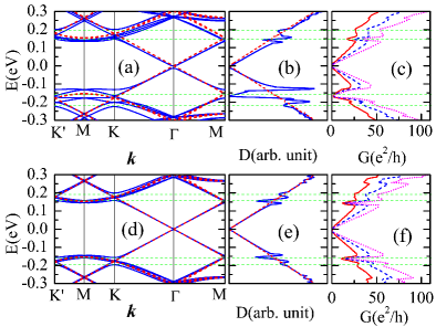
Figure B2: The calculated electronic structure of G/hBN with twist angle 0.5032^∘. (a), (b) and (c) are calculated with relaxation while (d), (e), and (f) are without lattice relaxation. (a) and (d) display the band structures; (b) and (e) are the density of states; (c) and (f) are the conductance without magnetic field. In the band structure and DOS, the red dashed lines denote the graphene monolayer results. In the conductance (c) and (f), the red solid, blue dashed, and magenta dot lines are calculated for device sizes 200nm$\times$200nm, 300nm$\times$300nm, and 400nm$\times$400nm, respectively.

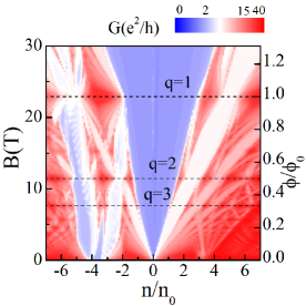
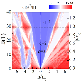
Figure B3: Landau fans for the longitudinal conductance for twist angles (a) 0.0^∘ and (b) 0.5032^∘.

Appendix C Appendix C: Edge dependence

Appendix D Appendix D: Details of magnetoconductivity

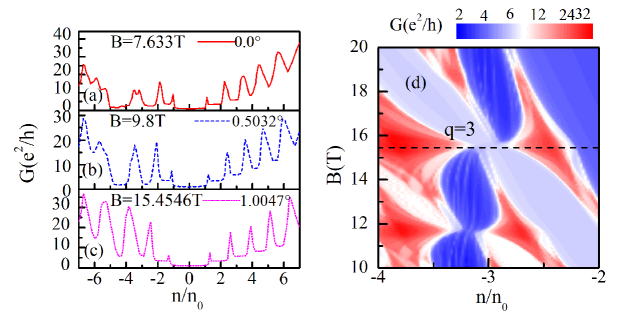
Figure D1: The conductances along the $q=3$ line in Fig. 2, Fig. B3(a) and Fig. B3(b) for magnetic fields B=7.633T, 9.8T, 15.4546T and the twist angles = 0.0^∘, 0.5032^∘ and 1.0047^∘. (d) Enlarged view of magnetic Dirac point closing in Fig. 2 around the $q=3$ line.

Appendix E Appendix E: Disorder effect

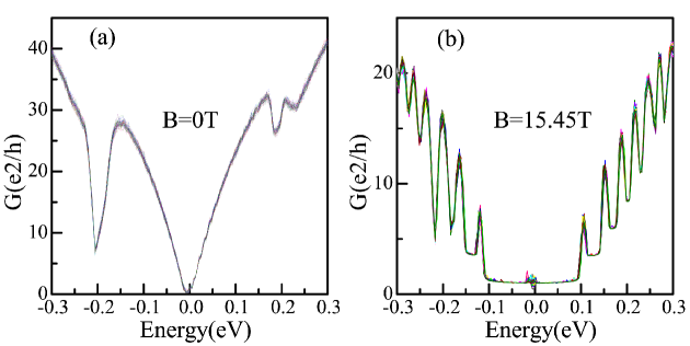
Figure E1: Conductance for 60 different realizations of the disorder for a twist angle = 1.0047^∘ with and without magnetic field. The site-diagonal random potential $v_{i}$ varies within the range [-$V_{0}$, $V_{0}$], where $V_{0}$=0.5eV. The main features (e.g., the secondary Dirac points) stay unchanged, though there are small fluctuations in the magnitude of the conductance.

Appendix F Appendix F: Antidot lattice

References

- (1) A. H. Castro Neto, F. Guinea, N. M. R. Peres, K. S. Novoselov, and A. K. Geim, The electronic properties of graphene, Rev. Mod. Phys. 81, 109-162 (2009).
- (2) M. J. Allen, V. C. Tung, and R. B. Kaner, Honeycomb Carbon: A Review of Graphene, Chem. Rev. 110, 132–145 (2010).
- (3) P. R. Wallace, The Band Theory of Graphite, Phys. Rev. 71, 622 (1947).
- (4) G. Xin, T. Yao, H. Sun, S. M. Scott, D. Shao, G. Wang, and J. Lian, Highly thermally conductive and mechanically strong graphene fibers, Science, 349, 1083-1087 (2015).
- (5) T. G. Pedersen, C. Flindt, J. Pedersen, N. A. Mortensen, A.-P. Jauho, and K. Pedersen, Graphene Antidot Lattices: Designed Defects and Spin Qubits, Phys. Rev. Lett. 100, 136804 (2008).
- (6) J. A. Fürst, J. G. Pedersen, C. Flindt, N. A. Mortensen, M. Brandbyge, T. G. Pedersen and A.-P. Jauho, Electronic properties of graphene antidot lattices, New J. Phys. 11, 095020 (2009).
- (7) J. A. Fürst, T. G. Pedersen, M. Brandbyge, and A.-P. Jauho, Density functional study of graphene antidot lattices: Roles of geometrical relaxation and spin, Phys. Rev. B 80, 115117 (2009).
- (8) R. Petersen, T. G. Pedersen, and A.-P. Jauho, Clar Sextet Analysis of Triangular, Rectangular, and Honeycomb Graphene Antidot Lattices, ACS Nano 5, 523 (2011).
- (9) F. Ouyang, S. Peng, Z. Liu, and Z. Liu, Bandgap Opening in Graphene Antidot Lattices: The Missing Half, ACS Nano 5, 4023-4030 (2011).
- (10) B. S. Jessen, L. Gammelgaard, M. R. Thomsen, D. M. A. Mackenzie, J. D. Thomsen, J. M. Caridad, E. Duegaard, K. Watanabe, T. Taniguchi, T. J. Booth, T. G. Pedersen, A.-P. Jauho, P. Bøggild, Lithographic band structure engineering of graphene, Nat. Nanotechnol. 14, 1029-1034 (2019).
- (11) J. G. Pedersen and T. G. Pedersen, Hofstadter butterflies and magnetically induced band-gap quenching in graphene antidot lattices, Phys. Rev. B 87, 235404 (2013).
- (12) G. J. Slotman, M. M. van Wijk, P.-L. Zhao, A. Fasolino, M. I. Katsnelson, and S. Yuan, Effect of Structural Relaxation on the Electronic Structure of Graphene on Hexagonal Boron Nitride, Phys. Rev. Lett. 115, 186801 (2015).
- (13) M. M. van Wijk, A. Schuring, M. I. Katsnelson, and A. Fasolino, Moiré Patterns as a Probe of Interplanar Interactions for Graphene on h-BN, Phys. Rev. Lett. 113, 135504 (2014).
- (14) M. Diez, J. P. Dahlhaus, M. Wimmer, and C.W. J. Beenakker, Emergence of Massless Dirac Fermions in Graphene’s Hofstadter Butterfly at Switches of the Quantum Hall Phase Connectivity, Phys. Rev. Lett. 112, 196602 (2014).
- (15) C. R. Dean, L. Wang, P. Maher, C. Forsythe, F. Ghahari, Y.Gao, J. Katoch, M. Ishigami, P. Moon, M. Koshino, T. Taniguchi, K. Watanabe, K. L. Shepard, J. Hone, and P. Kim, Hofstadter’s butterfly and the fractal quantum Hall effect in moiré superlattices, Nature 497, 598-602 (2013).
- (16) B. Hunt, J. D. Sanchez-Yamagishi, A. F. Young, M. Yankowitz, B. J. LeRoy, K. Watanabe, T. Taniguchi, P. Moon, M. Koshino, P. Jarillo-Herrero, R. C. Ashoori, Massive Dirac fermions and Hofstadter butterfly in a van der Waals heterostructure, Science 340, 1427-1431 (2013).
- (17) L. A. Ponomarenko, R. V. Gorbachev, G. L. Yu, D. C. Elias, R. Jalil, A. A. Patel, A. Mishchenko, A. S. Mayorov, C. R.Woods, J. R. Wallbank, M. Mucha-Kruczynski, B. A. Piot, M. Potemski, I. V. Grigorieva, K. S. Novoselov, F. Guinea, V. I. Fal’ko, and A. K. Geim, Cloning of Dirac fermions in graphene superlattices, Nature 497, 594-597 (2013).
- (18) J. Jung, A. M. DaSilva, A. H. MacDonald, and S. Adam, Origin of band gaps in graphene on hexagonal boron nitride, Nat. Commun. 6, 6308 (2015).
- (19) J. C. W. Song, A. V. Shytov, and L. S. Levitov, Electron Interactions and Gap Opening in Graphene Superlattices, Phys. Rev. Lett. 111, 266801 (2013).
- (20) L. Wang, Y. Gao, B. Wen, Z. Han, T. Taniguchi, K. Watanabe, M. Koshino, J. Hone, C. R. Dean, Evidence for a fractional fractal quantum Hall effect in graphene superlattices, Science 350, 1231-1234 (2015).
- (21) M. Yankowitz, Q. Ma, P. Jarillo- Herrero, and B. J. LeRoy, van der Waals heterostructures combining graphene and hexagonal boron nitride, Nat. Rev. Phys., 1, 112-125 (2019).
- (22) L. Balents, C. R. Dean, D. K. Efetov, and A. F. Young, Superconductivity and strong correlations in moiré flat bands, Nat. Phys. 16, 725-733 (2020).
- (23) C. R. Woods, L. Britnell, A. Eckmann, R. S. Ma, J. C. Lu, H. M. Guo, X. Lin, G. L. Yu, Y. Cao, R. V. Gorbachev, A. V. Kretinin, J. Park, L. A. Ponomarenko, M. I. Katsnelson, Yu. N. Gornostyrev, K.Watanabe, T. Taniguchi, C. Casiraghi, H-J. Gao, A. K. Geim and K. S. Novoselov, Commensurate-incommensurate transition in graphene on hexagonal boron nitride, Nat. Phys. 10, 451-456 (2014).
- (24) Y. Cao, V. Fatemi, S. Fang, K. Watanabe, T. Taniguchi, E. Kaxiras, and P. Jarillo-Herrero, Unconventional superconductivity in magic-angle graphene superlattices, Nature 556, 43-50 (2018).
- (25) Y. Cao, V. Fatemi, A. Demir, S. Fang, S. L. Tomarken, J. Y. Luo, J. D. Sanchez-Yamagishi, K. Watanabe, T. Taniguchi, E. Kaxiras, R. C. Ashoori and P. Jarillo-Herrero, Correlated insulator behaviour at half-filling in magic-angle graphene superlattices, Nature 556, 80-84 (2018).
- (26) T. Ahmed, K. Roy, S. Kakkar, A. Pradhan, and A. Ghosh, Interplay of charge transfer and disorder in optoelectronic response in Graphene/hBN/MoS2 van der Waals heterostructures, 2D Mater. 7, 025043 (2020).
- (27) X. Lin and J. Ni, Effective lattice model of graphene moiré superlattices on hexagonal boron nitride, Phys. Rev. B 100, 195413 (2019).
- (28) C. H. Lewenkopf, and E. R. Mucciolo, The recursive Green’s function method for graphene, J Comput Electron 12, 203–231 (2013).
- (29) J. Jung, A. Raoux, Z. H. Qiao, and A. H. MacDonald, Ab initio theory of moiré superlattice bands in layered two-dimensional materials, Phys. Rev. B 89, 205414 (2014).
- (30) P. Moon and M. Koshino, Electronic properties of graphene/hexagonal-boron-nitride moiré superlattice, Phys. Rev. B 90, 155406 (2014).
- (31) S.-C. Chen, R. Kraft, R. Danneau, K. Richter, and M.-H. Liu, Electrostatic superlattices on scaled graphene lattices, Communications Physics 3, 71, (2020).
- (32) J. Martin, N. Akerman, G. Ulbricht, T. Lohmann, Observation of electron-hole puddles in graphene using a scanning single-electron transistor, Nat. Phys. 4, 144-148 (2008); Y. Zhang, V. W. Brar, C. Girit, A. Zettl, M. F. Crommie, Origin of spatial charge inhomogeneity in graphene, Nat. Phys. 5, 722-726 (2009).
- (33) E. R. Mucciolo, A. H. Castro Neto, and C. H. Lewenkopf, Conductance quantization and transport gaps in disordered graphene nanoribbons, Phys. Rev. B 79, 075407 (2009); M. Evaldsson, I. V. Zozoulenko, H. Xu, and T. Heinzel, Edge-disorder-induced Anderson localization and conduction gap in graphene nanoribbons, Phys. Rev. B 78, 161407 (2008).
- (34) S. Yuan, R. Roldán, A.-P. Jauho, and M. Katsnelson, Electronic properties of disordered graphene antidot lattices, Phys. Rev. B 87, 085430 (2013).
- (35) S. Yuan, F. Jin, R. Roldán, A.-P. Jauho, and M. I. Katsnelson, Screening and collective modes in disordered graphene antidot lattices, Phys. Rev. B 88, 195401 (2013).
- (36) V. Hung Nguyen, M. Chung Nguyen, H.-V. Nguyen, and P. Dollfus, Disorder effects on electronic bandgap and transport in graphene-nanomesh-based structures, J. Appl. Phys. 113, 013702 (2013).
- (37) X. Ji, J. Zhang, Y. Wang, H. Qian, and Z. Yu, Influence of edge imperfections on the transport behavior of graphene nanomeshes, Nanoscale 5, 2527 (2013).
- (38) S. R. Power and A.-P. Jauho, Electronic transport in disordered graphene antidot lattice devices, Phys. Rev. B 90, 115408 (2014).
- (39) N. R. Finney, M. Yankowitz, L. Muraleetharan, K. Watanabe, T. Taniguchi , C. R. Dean, and J. Hone, Tunable crystal symmetry in graphene-boron nitride heterostructures with coexisting moiré superlattices, Nat. Nanotechnol. 14, 1029-1034 (2019).
- (40) Z. Wang, Y. B. Wang, J. Yin, E. Tóvári, Y. Yang, L. Lin, M. Holwill, J. Birkbeck, D. J. Perello, S. Xu, J. Zultak, R. V. Gorbachev, A. V. Kretinin, T. Taniguchi, K. Watanabe, S. V. Morozov, M. Anđelković, S. P. Milovanović, L. Covaci, F. M. Peeters, A. Mishchenko, A. K. Geim, K. S. Novoselov, V. I. Fal’ko, A. Knothe, C. R. Woods, Composite super-moiré lattices in double-aligned graphene heterostructures, Science Advances 5, 8897 (2019).
- (41) L. Wang, S. Zihlmann, M.-H. Liu, P. Makk, K. Watanabe, T. Taniguchi, A. Baumgartner, and C. Schönenberger, New Generation of Moiré Superlattices in Doubly Aligned hBN/Graphene/hBN Heterostructures, Nano Lett. 19, 2371-2376 (2019).
- (42) M. Anđelković, S. P. Milovanović, L. Covaci, and F. M. Peeters, Double Moiré with a Twist: Supermoiré in Encapsulated Graphene, Nano Letters 20, 979-988 (2020).
- (43) N. N. T. Nam and M. Koshino, Lattice relaxation and energy band modulation in twisted bilayer graphene, Phys. Rev. B 96, 075311 (2017).
- (44) S. Fang, S. Carr, M. A. Cazalila, and E. Kaxiras, Electronic structure theory of strained two-dimensional materials with hexagonal symmetry, Phys. Rev. B 98, 075106 (2018).