ITEP-TH-28/20

Wiedemann-Franz laws and $Sl(2,\mathbb{Z})$ duality in AdS/CMT holographic duals and one-dimensional effective actions for them

Dmitry Melnikov^a,b and Horatiu Nastase^c

^aInternational Institute of Physics, Universidade Federal do Rio Grande do Norte,

Campus Universitário, Lagoa Nova, Natal-RN 59078-970, Brazil

^bInstitute for Theoretical and Experimental Physics,

B. Cheremushkinskaya 25, Moscow 117218, Russia

^cInstituto de Física Teórica, UNESP-Universidade Estadual Paulista

R. Dr. Bento T. Ferraz 271, Bl. II, Sao Paulo 01140-070, SP, Brazil

Abstract

1 Introduction

In classical Fermi liquid theory in 2+1 dimensions, one obtains the Wiedemann-Franz law for the ratio of the off-diagonal heat transport coefficient $\kappa_{xy}/T$ to the Hall conductivity in the $T\rightarrow 0$ limit,

$$\frac{\kappa_{xy}/T}{\sigma_{xy}}\rightarrow\frac{\pi^{2}}{3}\left(\frac{k_{B}}{e}\right)^{2}.$$ (1.1)

However, it was known since the work of Kane and Fisher [1] that the right-hand side, called the Lorenz number $L$, can in general be multiplied by some object, which later, in the work of Read and Green for the Fractional Quantum Hall Effect (FQHE) [2] was identified with a central charge $c$. But in such more complicated systems, like systems described by conformal Abelian Chern-Simons analyzed in [3], there is an action of an $Sl(2,\mathbb{Z})$ symmetry on them, including a $T$ and an $S$ generator. The $S$ generator acts via the particle-vortex symmetry, which can be defined as in terms of field theory in [4], and better defined in [5] (at the level of the path integral), and results in an action on the complex electrical conductivity $\sigma=\sigma_{xy}+i\sigma_{xx}$.

It is then of interest to see what we can obtain obtain for the Wiedemann-Franz law and $Sl(2,\mathbb{Z})$ symmetry in systems described holographically, via the AdS/CMT correspondence (see for instance the book [6] for a review). Transport in 2+1 dimensional case was discussed in a number of papers: the first results for systems in magnetic field were obtained in [7, 8]. In [8], the symmetry of the charge and heat transport coefficients with respect to the electric-magnetic duality action was observed in both the holographic and magnetohydronamic approaches. One of the questions that we will address here is the relations of those results with the above classical Wiedemann-Franz law, with $L=\pi^{2}/3$, as well as with the non-Fermi liquid extension, with a nontrivial central charge $c$ coefficient.

We will also consider a slightly more general holographic setup describing a disordered system in the presence of a nontrivial electric charge density $\rho$ and magnetic field $B$, as well as a nontrivial $\theta F_{\mu\nu}\tilde{F}^{\mu\nu}$ term, corresponding to Chern-Simons in 3 dimensions, as in [9] (following [10] and [11]). We will analyze the Lorenz number $L$ coming from that calculation, as well as the analogous law for the dissipative components $xx$, and the action of the $Sl(2,\mathbb{Z})$ on the transport coefficients and the laws. We will show that the dependence of the conductivities from the disorder in the holographic model match precisely the hydrodynamic analysis of [8] if the rescaled disorder parameter is replaced by the inverse scattering time. Even though we work with DC conductivities, the frequency dependence can be obtained by a shift of the disorder parameter.

We show that the coupling constants of the 3+1 dimensional gravity Lagrangian can be thought of as bare values of the conductivity, as in effective two dimensional sigma models of conductivity in disordered systems. Magnetic field is a relevant perturbation, which drives the system to a IR fixed point, corresponding to the quantum Hall regime, with zero direct conductivity. The electric-magnetic duality restricts this flow to the fundamental domain of $Sl(2,\mathbb{Z})$. Integer shifts of the theta term translate the fundamental domain in the upper half plane.

As far as the Wiedmann-Franz law is concerned we find that at the fixed point with no disorder the most interesting quantity is not the thermal conductivity $\kappa$, but rather the heat conductivity $\bar{\kappa}$, so that at low temperature one gets the modified Lorenz number

$$\bar{L}\ \equiv\ \frac{\bar{\kappa}/T}{\sigma}\ =\ \frac{\pi}{3}\,cg_{4}^{2}+O(T)\,.$$ (1.2)

in terms of the centeral charge $c$ and the gravity coupling $g_{4}$. In the normalization of [8] $cg_{4}^{2}=\pi$ so $\bar{L}$ takes the value of the classical Lorenz number (1.1). The interesting part is that this specific normalization is the self-dual point of the model, according to [12]. Since the duality exchanges $\kappa_{xy}\leftrightarrow\bar{\kappa}_{xy}$, $\bar{L}$ calculated in the gravity dual actually measures $L$ in the weakly coupled gauge theory. This feature does not hold for a generic holographic model, and gravity is not expected to capture the weak coupling regime of the dual theory. However, if self-duality is exact, it should provide a window into weak coupling.

The strong coupling value of the Lorenz number is

$$L\ \equiv\ \frac{\pi}{3}\frac{c}{g_{4}^{2}}\frac{1}{\sigma_{xy}^{2}}+O(T)\,.$$ (1.3)

At the self-dual point it is equal to $c^{2}/(3\sigma_{xy}^{2})$.

In the case of direct conductivities, similar result holds in the limit of zero magnetic field, and then zero disorder, in which case the modified Lorenz number has a finite value ${\bar{L}}_{xx}=\pi/3(cg_{4}^{2})$. This is again mapped to the weak coupling value by the duality.

Further, in [13], the Wiedemann-Franz law was analyzed from the point of view of $SYK_{q}$ generalizations of the SYK model for $q$ fermion interactions, both in $d$ dimensional lattices of $SYK_{q}$ models, and in the gravity duals corresponding to the same physics. For the special choice of intersite coupling the Lorenz number of the $SYK_{q}$ model was shown to be given by

$$L\ =\ \frac{4\pi^{2}}{3q^{2}}\,,$$ (1.4)

with $q=2$ corresponding to the free theory point. However, this result was not reproduced by the gravity calculations.

A 0+1 dimensional effective action generalizing the Schwarzian action for the standard SYK model was also found in [13] for complex fermions with charge. We will show that it can be used to directly find the transport in the charged $SYK_{q}$ models. We will also show how it can be matched to the holographic calculation in the large $q$ limit. We will find that the ratio of the heat and charge susceptibilities is also expressed as

$$\frac{\gamma}{K}\ =\ \frac{\pi}{3}cg_{4}^{2}\,,$$ (1.5)

at zero magnetic field. Moreover, we will show that we can extend the 0+1 dimensional effective action to one that is selfdual under electric-magnetic S duality, and we can also add a $\theta$ term corresponding to the T operation, thus arriving at an $Sl(2,\mathbb{Z})$ invariant form.

The paper is organized as follows. In section 2 we define the transport coefficients, and describe the general expectations for the Wiedemann-Franz laws. In section 3 we first find the holographic transport coefficients and W-F laws, then describe the effect of $Sl(2,\mathbb{Z})$ on them, and finally generalize the calculation of [8] to the case of nontrivial central charge $c$. In section 4 we calculate the transport coefficients from the 0+1 dimensional generalized Schwarzian effective action, and compare with the holographic calculations. In section 5 we write the self-dual version of the 0+1 dimensional effective action, and find the $\theta$ term for the same, and in section 6 we conclude. In Appendix A we review the action of particle-vortex duality, and in Appendix B – an alternative calculation of conductivities from the effective action of the generalized SYK models.

2 Wiedemann-Franz laws in condensed matter and general theory

2.1 Definition of transport coefficients in various dimensions

In this paper, we will be interested in electric and heat transport, and the corresponding transport coefficients.

Transport coefficients are defined as the coefficients for the linear response (electric current $\vec{J}$, heat current $\vec{Q}$, etc.) of the material to external fields: external electric field $\vec{E}$ and external temperature gradient $\vec{\nabla}T$ in our case. One can write then (in the convention in [8]) the matriceal relation

$$\begin{pmatrix}\vec{J}\\ \vec{Q}\end{pmatrix}=\begin{pmatrix}\hat{\sigma}&\hat{\alpha}\\ T\hat{\alpha}&\hat{\bar{\kappa}}\end{pmatrix}\begin{pmatrix}\vec{E}\\ -\vec{\nabla}T\end{pmatrix}\;,$$ (2.1)

where $\hat{\sigma}$ is the matrix of electric conductivities, $\hat{\alpha}$ is the matrix of thermoelectric conductivites and the matrix of thermal conductivities is

$$\hat{\kappa}=\hat{\bar{\kappa}}-T\hat{\alpha}\hat{\sigma}^{-1}\hat{\alpha}.$$ (2.2)

One can also define the thermoelectric power coefficient

$$\hat{\theta}=-\hat{\sigma}^{-1}\hat{\alpha}\;,$$ (2.3)

so that the Nernst coefficient is

$$\nu=\frac{\theta_{xy}}{B}.$$ (2.4)

Note that instead of using matrices, in the specific case of isotropic coefficients, i.e., that $\sigma_{xx}=\sigma_{yy}$ and $\sigma_{xy}=-\sigma_{yx}$ and similar for all the other transport coefficients, so

$$\sigma=\sigma_{xx}{\,\hbox{1\kern-2.27621ptl}}+\sigma_{xy}{\bf\epsilon}\;,\;\;\alpha=\alpha_{xx}{\,\hbox{1\kern-2.27621ptl}}+\alpha_{xy}{\bf\epsilon}\;,\;\;\kappa=\kappa_{xx}{\,\hbox{1\kern-2.27621ptl}}+\kappa_{xy}{\bf\epsilon}\;,$$ (2.5)

we can use complex quantities,

$$\sigma\equiv\sigma_{xy}+i\sigma_{xx}\;,\;\;A\equiv\alpha_{xy}+i\alpha_{xx}\;,\;\;K\equiv\kappa_{xy}+i\kappa_{xx}\;,$$ (2.6)

and obtain the same results, in particular

$$\frac{\kappa_{xx}}{T} = \frac{\bar{\kappa}_{xx}}{T}-\frac{\alpha_{xx}^{2}\sigma_{xx}+2\alpha_{xx}\alpha_{xy}\sigma_{xy}-\sigma_{xx}\alpha_{xy}^{2}}{\sigma_{xx}^{2}+\sigma_{xy}^{2}}$$ (2.7)

$$\frac{\kappa_{xy}}{T} = \frac{\bar{\kappa}_{xy}}{T}-\frac{\alpha_{xy}^{2}\sigma_{xy}+2\alpha_{xx}\alpha_{xy}\sigma_{xx}-\sigma_{xy}\alpha_{xx}^{2}}{\sigma_{xx}^{2}+\sigma_{xy}^{2}}.$$ (2.8)

One can calculate the above transport coefficients also from the diffusivity coefficients $D$ and the susceptibilities $\chi$ in momentum space (here we follow [13] – one of the original references is [14]). In a general dimension, one defines $\chi_{s}$ from $\chi$ as

$$\chi(k,\omega)=[i\omega(-i\omega+Dk^{2})^{-1}+1]\chi_{s}\;,$$ (2.9)

where

$$D=\begin{pmatrix}D_{1}&0\\ 2\pi{\cal E}(D_{1}-D_{2})&D_{2}\end{pmatrix}$$ (2.10)

and then the matrix of transport coefficients is

$$\begin{pmatrix}\sigma&\alpha\\ \alpha T&\bar{\kappa}\end{pmatrix}=D\chi_{s}.$$ (2.11)

Note that in the above we can also consider either $\sigma,\alpha,\bar{\kappa}$ and $D$ to be matrices, or equivalently, to be complex objects, with $D=D_{xy}+iD_{xx}$. Since $\chi_{s}$ are thermodynamical quantities, they are the same for $xx$ and $xy$ components, so by taking the real and imaginary parts of the above equation (understood as a complex equation), we obtain

$$\begin{pmatrix}\sigma_{xy}&\alpha_{xy}\\ \alpha_{xy}T&\bar{\kappa}_{xy}\end{pmatrix}=D_{xy}\chi_{s}\;,\;\;\;\begin{pmatrix}\sigma_{xx}&\alpha_{xx}\\ \alpha_{xx}T&\bar{\kappa}_{xx}\end{pmatrix}=D_{xx}\chi_{s}.$$ (2.12)

2.2 General theory expectations and Wiedemann-Franz laws

In classical condensed matter in 2+1 dimensions, Fermi liquid theory obtains the Wiedemann-Franz law for the off-diagonal (”Hall”, or Leduc-Righi (LR)) heat transport coefficient $\kappa_{xy}$ and the Hall electrical conductivity: at temperature $T\rightarrow 0$,

$$\frac{\kappa_{xy}/T}{\sigma_{xy}}\rightarrow\frac{\pi^{2}}{3}.$$ (2.13)

More precisely, restoring all dimensions, there is also a $k_{B}^{2}$ on the right-hand side, and the corresponding object is called the Lorenz number.

Now, for some materials, the $T\rightarrow 0$ limit of $\kappa_{xy}/\sigma_{xy}$ has a different form. In the (Fractional) Quantum Hall Effect, corresponding to an interacting system, the question is why is there a different coefficient in the W-F law, rather than $\pi^{2}/3$? Kane and Fisher [1] have argued that there are different Landau levels, meaning different edge modes. There is also the filling fraction appearing both in $\kappa_{xy}$ and in $\sigma_{xy}$, but it cancels in the ratio.

More precisely, in the work of Kane and Fisher [1], it is shown that the ratio of the thermal and electric Hall conductivities can be expressed as

$$\frac{\kappa_{xy}}{\sigma_{xy}}\ =\ \frac{\sum_{a}\eta_{a}}{\sum_{a}t_{a}^{2}\eta_{a}}\frac{\pi^{2}}{3}T\;,$$ (2.14)

where $\eta_{a}$ are inverse eigenvalues of an $N\times N$ matrix $K_{ab}$ characterizing a given topological order (phase) at the $N$th level of the Haldane-Halperin hierarchy. Numbers $t^{a}$ are charges of elementary quasiparticle excitations at this level (for example charges of an electron or a hole excitations). Before diagonalization these numbers are typically assumed to be $t_{a}=1$, which means that possible bound states of electrons are ignored. After diagonalization $t_{a}$ are some numbers depending on $K_{ab}$. In other words,

$$\frac{\kappa_{xy}}{\sigma_{xy}}\ =\ \frac{\sum_{ab}\eta_{ab}}{\sum_{ab}K^{-1}_{ab}}\frac{\pi^{2}}{3}T\;,$$ (2.15)

In [1] it is somewhat assumed that $\eta_{a}=\pm 1$ (although it does not seem to be a generic property [15]) so each of these numbers represent edge modes moving in the direction prescribed by the magnetic field $\eta=1$, or in the opposite direction $\eta=-1$. Each such mode contribuites a unit of heat conductivity and $t^{2}_{a}$ units of electric conductivity, summed algebraically. For example, if all the modes propagate in the same direction then $\sum_{a}\eta_{a}=N$ counts the number of channels. Also, if all $t_{a}=1$ (after diagonalization), the Lorenz number takes its classical value, while its deviation from that value depends on the structure of the matrix $K_{ab}$.

Later, in the work of Read and Green [2], it was argued that in the case of a 2+1 dimensional FQHE system with 2 edges, the edge modes control all transport, and we can construct:

-a spin analog of electric Hall conductivity, and obtain, for the p-wave paired state, and with the spin in units of $\hbar$,

$$\sigma_{xy}^{s}=\frac{m}{h}\;,$$ (2.16)

where $h$ is the Planck constant (=$2\pi\hbar$) and $m$ is a integer winding number equal to $\pm 1$ in a weak-pairing phase. The electric conductivity should have similar properties. Since the electric charge is $e$, we expect the electric conductivity to also be $\sigma_{xy}\propto e^{2}$.

-the Hall (or LR) heat conductivity

$$\kappa_{xy}=c\frac{\pi^{2}}{3h}T\;,$$ (2.17)

where $c$ is the (Virasoro) central charge of the 1+1 dimensional edge conformal field theory (including the edge modes of the FQHE) [16, 17, 18]. In the case that the 2 edge modes move in different directions, the central charge should be of the difference between right- and left-moving theories. Note however that for a Majorana fermion $c=1/2$, so a priori $c$ could be half-integer.

That means that the Lorenz number is proportional to $c$. Note that the central charge $c$ is for the 1+1 dimensional edge of the 2+1 dimensional field theory; however, if only the edge modes are relevant (as in the case of the FQHE, or for Chern-Simons models), it can be thought of as the central charge (or number of degrees of freedom in a generalized sense) for the field theory. In dimensions higher than 2, the central charge is related to the trace anomaly $\langle{T^{\mu}}_{\mu}\rangle$, or anomaly in conformal invariance (but is not a central charge in the Virasoro algebra anymore).

It was also proposed that for the normal (dissipative) heat conductivity,

$$\kappa_{xx}=\kappa_{yy}\sim\frac{\pi^{2}}{3h}\frac{T}{g^{2}}\;,$$ (2.18)

where $g$ is the coupling in the two-dimensional nonlinear sigma model for disordered electron systems, e.g. [19].

Moreover, in [8] it was shown that in fact, in general, and in a holographic model (dyonic black hole in $AdS_{4}$), all transport coefficients come from a universal quantity

$$\sigma_{Q}=\frac{4e^{2}}{h}\Phi_{\sigma}.$$ (2.19)

In particular $\sigma_{xx}=\sigma_{Q}+...$, and then

$$\kappa_{xx}=\frac{\Phi_{\sigma}}{h}k_{B}^{2}T\left(\frac{\epsilon+P}{k_{B}T\rho}\right)[...]\;,$$ (2.20)

where the bracket $[...]$ goes to 1 in a certain limit.

Then we expect that there should be an analog of the Wiedemann-Franz law for the dissipative components in the case of these nontrivial strongly coupled systems (FQHE-like), so

$$\frac{\kappa_{xx}/T}{\sigma_{xx}}\sim(...)\frac{\pi^{2}k_{B}^{2}}{3}.$$ (2.21)

3 $Sl(2,\mathbb{Z})$ duality on transport coefficients and Wiedemann-Franz law for AdS/CMT holographic models

3.1 AdS/CMT holographic models and results for transport coefficients

AdS/CMT models are usually phenomenological holographic models. To describe 2+1 dimensional matter with charge and heat transport, we need to consider a 3+1 dimensional gravitational solution in a phenomenological theory with a gauge field and charged black hole solutions in an AdS background.

The 3+1 dimensional (holographic bulk) gravitational model contains gravity, 3 scalars and a vector. The action is

$$S = \int d^{4}x\sqrt{-g}\left[\frac{1}{16\pi G_{N}}\left(R-\frac{1}{2}\left[(\partial_{\mu}\phi)^{2}+\Phi(\phi)\left((\partial_{\mu}\chi_{1})^{2}+(\partial_{\mu}\chi_{2})^{2}\right)\right]-V(\phi)\right)\right.$$ (3.2)

$$\left.-\frac{Z(\phi)}{g_{4}^{2}}F_{\mu\nu}^{2}-W(\phi)F_{\mu\nu}\tilde{F}^{\mu\nu}\right].$$

Note that there are two ”axions” $\chi_{1},\chi_{2}$ that are usually ignored, by putting $\Phi(\phi)=0$, but they are necessary if we want to have dissipative charge and heat transport, since we need to break translational invariance in the $x$ and $y$ directions, achieved by having a linear background for the axions. Alternatively, the translational symmetry breaking can be introduced via a ”holographic lattice”, that is considering a metric with explicit dependence of spatial coordinates, as for example in [20]. We will not take this path here.

Considering a black hole solution with certain asymptotics of the perturbed AdS type in the gravity sector, and then adding boundary sources for the perturbation in $\vec{\nabla}T/T$, the electric and magnetic fields $\vec{E},\vec{B}$ and charge density $\rho$, we can calculate the transport coefficients as follows (see [21] for the original idea). We can calculate certain fluxes $\vec{\cal J}$ and $\vec{\cal Q}$ (modifications of the electric current $\vec{j}$ and heat current $\vec{Q}$) that are $r$-independent, so can be calculated at the horizon of the black hole, from the metric fluctuations induced at the horizon by the presence of varying sources for $\vec{E}$ and $\vec{\nabla}T/T$, in the presence of constant $\vec{B}$ and $\rho$. Then the transport coefficients are the linear response coefficients and were found to be [9]

$$\sigma_{xx} = e^{2V}k^{2}\Phi\frac{(2\kappa_{4}^{2})\frac{g_{4}^{4}}{Z^{2}}\rho^{2}+(2\kappa_{4}^{2})B^{2}+\frac{g_{4}^{2}}{Z}e^{2V}k^{2}\Phi}{(2\kappa_{4}^{2})^{2}\frac{g_{4}^{4}}{Z^{2}}B^{2}\rho^{2}+(2\kappa_{4}^{2}B^{2}+\frac{g_{4}^{2}}{Z}e^{2V}k^{2}\Phi)^{2}}$$ (3.3)

$$= \frac{e^{2V}k^{2}\Phi}{(2\kappa_{4}^{2})B^{2}}\frac{1+\frac{B^{2}Z^{2}}{\rho^{2}g_{4}^{4}}+\frac{Ze^{2V}k^{2}\Phi}{g_{4}^{2}2\kappa_{4}^{2}\rho^{2}}}{1+\left(\frac{BZ}{\rho g_{4}^{2}}+\frac{e^{2V}k^{2}\Phi}{2\kappa_{4}^{2}B\rho}\right)^{2}}$$ (3.4)

$$\sigma_{xy} = 2\kappa_{4}^{2}\frac{\rho}{B}\frac{2\kappa_{4}^{2}\frac{g_{4}^{4}}{Z^{2}}\rho^{2}+2\kappa_{4}^{2}B^{2}+2\frac{g_{4}^{2}}{Z}e^{2V}k^{2}\Phi}{(2\kappa_{4}^{2})^{2}\frac{g_{4}^{4}}{Z^{2}}B^{2}\rho^{2}+(2\kappa_{4}^{2}B^{2}+\frac{g_{4}^{2}}{Z}e^{2V}k^{2}\Phi)^{2}}-4W$$ (3.5)

$$= \frac{\rho}{B}\frac{1+\frac{B^{2}Z^{2}}{\rho^{2}g_{4}^{4}}+2\frac{Ze^{2V}k^{2}\Phi}{g_{4}^{2}2\kappa_{4}^{2}\rho^{2}}}{1+\left(\frac{BZ}{\rho g_{4}^{2}}+\frac{e^{2V}k^{2}\Phi}{2\kappa_{4}^{2}B\rho}\right)^{2}}-4W.$$ (3.6)

for the electric conductivities,

$$\frac{\bar{\kappa}_{xx}}{T} = (2\kappa_{4}^{2})s^{2}\frac{g_{4}^{2}\left[(2\kappa_{4}^{2})B^{2}Z+g_{4}^{2}e^{2V}k^{2}\Phi\right]}{(2\kappa_{4}^{2})^{2}g_{4}^{4}\rho^{2}B^{2}+((2\kappa_{4}^{2})B^{2}Z+g_{4}^{2}e^{2V}k^{2}\Phi)^{2}}$$ (3.7)

$$= \frac{s^{2}}{\rho^{2}}\frac{\frac{Z}{g_{4}^{2}}+\frac{e^{2V}k^{2}\Phi}{(2\kappa_{4}^{2})B^{2}}}{1+\left(\frac{BZ}{\rho g_{4}^{2}}+\frac{e^{2V}k^{2}\Phi}{2\kappa_{4}^{2}B\rho}\right)^{2}}$$ (3.8)

$$\frac{\bar{\kappa}_{xy}}{T} = (2\kappa_{4}^{2})s^{2}\frac{g_{4}^{2}(2\kappa_{4}^{2})g_{4}^{2}\rho B}{(2\kappa_{4}^{2})^{2}g_{4}^{4}\rho^{2}B^{2}+((2\kappa_{4}^{2})B^{2}Z+g_{4}^{2}e^{2V}k^{2}\Phi)^{2}}$$ (3.9)

$$= \frac{s^{2}}{\rho B}\frac{1}{1+\left(\frac{BZ}{\rho g_{4}^{2}}+\frac{e^{2V}k^{2}\Phi}{2\kappa_{4}^{2}B\rho}\right)^{2}}\;,$$ (3.10)

for the heat conductivities, and

$${\alpha_{xx}} = s\rho\frac{(2\kappa_{4}^{2})\frac{g_{4}^{4}}{Z^{2}}e^{2V}k^{2}\Phi}{(2\kappa_{4}^{2})^{2}\frac{g_{4}^{4}}{Z^{2}}B^{2}\rho^{2}+(2\kappa_{4}^{2}B^{2}+\frac{g_{4}^{2}}{Z}e^{2V}k^{2}\Phi)^{2}}$$ (3.11)

$$= \frac{s}{\rho B^{2}}\frac{\frac{e^{2V}k^{2}\Phi}{(2\kappa_{4}^{2})}}{1+\left(\frac{BZ}{\rho g_{4}^{2}}+\frac{e^{2V}k^{2}\Phi}{2\kappa_{4}^{2}B\rho}\right)^{2}}$$ (3.12)

$${\alpha_{xy}} = 2\kappa_{4}^{2}{sB}\frac{(2\kappa_{4}^{2})\frac{g_{4}^{4}}{Z^{2}}\rho^{2}+(2\kappa_{4}^{2})B^{2}+\frac{g_{4}^{2}}{Z}e^{2V}k^{2}\Phi}{(2\kappa_{4}^{2})^{2}\frac{g_{4}^{4}}{Z^{2}}B^{2}\rho^{2}+(2\kappa_{4}^{2}B^{2}+\frac{g_{4}^{4}}{Z^{2}}e^{2V}k^{2}\Phi)^{2}}$$ (3.13)

$$= \frac{s}{B}\frac{1+\frac{B^{2}Z^{2}}{\rho^{2}g_{4}^{4}}+\frac{Ze^{2V}k^{2}\Phi}{g_{4}^{2}2\kappa_{4}^{2}\rho^{2}}}{1+\left(\frac{BZ}{\rho g_{4}^{2}}+\frac{e^{2V}k^{2}\Phi}{2\kappa_{4}^{2}B\rho}\right)^{2}}\;,$$ (3.14)

for the thermoelectric conductivities, where we restored the dependence on the Newton’s constant $\kappa_{4}$ and of $g_{4}^{2}$ with respect to [9]. Here $e^{2V},\Phi,Z$ and $W$ are defined at the horizon $r_{H}$ of the black hole, with $e^{2V}$ being the warp factor for the spatial part of the holographic boundary, $(x,y)$.

Note that the effective squared coupling is $g_{4}^{2}/Z(r_{H})$. Also note that at $\Phi(r_{H})=0$, $\sigma_{xx}\rightarrow 0$, which means that

$$\frac{\bar{\kappa}_{xx}/T}{\sigma_{xx}}\rightarrow\infty.$$ (3.15)

Let us make a few comments about this limit.

In a translationally invariant (clean) system without magnetic field both charge and heat conductivities are infinite, because the electrons can move without dissipation. This can be seen by taking first the limit $B\to 0$ and then $\Phi(r_{H})\to 0$ in the above equations. For finite magnetic field, the gravity system should correspond to a strongly coupled theory of FQHE type on the holographic boundary. In such a system the FQHE bulk electron states are localized, unable to transport electric charge and, similarly, heat. Strictly speaking, for localization one needs disorder in the bulk that would create energy levels for the electrons to occupy. For this reason, in a perfectly clean limit, one expects that there is essentially no quantum Hall effect and the sequence of plateaux in the $\sigma_{xx}$ is replaced by a continuous dependence $\rho/B$. The sequence of peaks in $\sigma_{xx}$ in this limit can either be replaced by a finite value or vanish. In a real experiment one expects to observe finite $\sigma_{xx}$: first, because the peaks are broad and second, because edge currents can contribute to $\sigma_{xx}$. In the holographic model, for $\Phi(r_{H})=0$, $\sigma_{xx}=0$.

In the meantime longitudinal heat conductivity does not vanish in the limit $\Phi(r_{H})\to 0$. One notices that heat can also be transported by phonons, which do not carry charge. Phonons do not couple to the magnetic field, and we will see that for small temperature $\kappa_{xx}$ is ${\cal O}(T)$, independent from $\rho$ and $B$, consistent with the phonon interpretation.

Another possible interpretation of (3.15) in the clean limit $\Phi(r_{H})\to 0$ is that the gravity dual describes an ensemble average over a disorder. Upon averaging, the translational invariance is restored in the system, but $\sigma_{xx}$ remains vanishing because it is so in every ensemble representative. Again, non-zero $\kappa_{xx}$ can be attributed to phonons. The ensemble average interpretation is consistent with the effective SYK-like description of the dyonic black hole that we discuss in the following part of the work.

In the general case, the modified longitudinal Wiedemann-Franz law (the longitudinal Lorenz number $\bar{L}_{xx}$) reads

$$\bar{L}_{xx}\ \equiv\ \frac{\bar{\kappa}_{xx}/T}{\sigma_{xx}}=\frac{s^{2}}{\rho^{2}}\frac{\frac{Z}{g_{4}^{2}}+\frac{e^{2V}k^{2}\Phi}{(2\kappa_{4}^{2})B^{2}}}{\frac{e^{2V}k^{2}\Phi}{(2\kappa_{4}^{2})B^{2}}\left[1+\frac{B^{2}Z^{2}}{\rho^{2}g_{4}^{4}}+\frac{Ze^{2V}k^{2}\Phi}{g_{4}^{2}2\kappa_{4}^{2}\rho^{2}}\right]}\,.$$ (3.16)

Note that we use $\bar{\kappa}_{xx}$ instead of the usual $\kappa_{xx}$. The explanation will be given in the subsection after next.

If one takes the limit $B\to 0$, both the heat and the electric conductivities are infinite, but their ratio is finite for any $\Phi$.

$$\bar{L}_{xx}\ =\ \frac{s^{2}}{\rho^{2}+\frac{Ze^{2V}k^{2}\Phi}{g_{4}^{2}2\kappa_{4}^{2}}}\,.$$ (3.17)

We will see in the subsection after next that, with the assumption that we can use the dyonic black hole for the same calculation, we can use the equations $s=c\alpha^{2}$, $\rho=\frac{c}{\pi}\alpha\mu$, $c\frac{g_{4}^{2}}{Z}=\pi$ and $\frac{\mu^{2}}{\alpha^{2}}-\frac{B^{2}}{\alpha^{4}}-3=\frac{4\pi T}{\alpha}$, and as $T\rightarrow 0$, cancel the dependence on $\alpha$, to obtain

$$\frac{s^{2}}{\rho^{2}+\frac{B^{2}Z^{2}}{g_{4}^{2}}}=\frac{\pi^{2}}{3}+{\cal O}(T)\,.$$ (3.18)

It looks then that also in this case $\bar{L}_{xx}=\pi^{2}/3$ for $T\to 0$, at least for $\Phi\rightarrow 0$. That is possible if we take first $B\rightarrow 0$, and then $\Phi\rightarrow 0$. This might seem odd, given that $\Phi$ is a property of the model, whereas $B$ is an external field, but one can certainly take a very small but nonzero $\Phi$, yet $B=0$, in which case we obtain the desired result.

For the Hall components, the modified transverse Lorenz number can be calculated for $\Phi(r_{H})=0$. In this case, we obtain

$$\sigma_{xy} = \frac{\rho}{B}-W(r_{H})\,,$$ (3.19)

$$\frac{\bar{\kappa}_{xy}}{T} = s^{2}\frac{\rho/B}{\rho^{2}+\frac{B^{2}Z(r_{H})^{2}}{g_{4}^{4}}}\;,$$ (3.20)

so the modified transverse Lorenz number is

$$\bar{L}\equiv\frac{\kappa_{xy}/T}{\sigma_{xy}}=\frac{\rho/B}{\rho/B-4W}\frac{s^{2}}{\rho^{2}+\frac{B^{2}Z^{2}}{g_{4}^{4}}}.$$ (3.21)

For $W(r_{H})=0$ (no topological term, or see the discussion in the next subsection), and absorbing $Z(r_{H})$ into $g_{4}^{2}$, we obtain

$$\bar{L}=\frac{s^{2}}{\rho^{2}+\frac{B^{2}}{g_{4}^{4}}}.$$ (3.22)

We notice the similar structure of the Lorentz numbers (3.17) and (3.22), in the longitudinal and transverse channels. Magnetic field in the transverse conductivity plays a role similar to disorder in the direct one. In the limit $B=\Phi(r_{H})=0$ the Lorentz numbers are equal. However, at this moment, they do not yet look like the expected formula from the previous section.

What about the usual Lorenz numbers, in terms of the thermal conductivity $\kappa$, instead of the heat conductivity $\bar{\kappa}$? The transition between the two is given by (2.8). It only makes sense to cite the result at $W(r_{h})=0$,

$$\frac{\kappa_{xx}}{T} = \frac{s^{2}}{\rho}\frac{\frac{\rho g_{4}^{2}}{Z}+\frac{k^{2}e^{2V}\Phi}{2\kappa_{4}^{2}\rho}}{B^{2}+\left(\frac{\rho g_{4}^{2}}{Z}+\frac{k^{2}e^{2V}\Phi}{2\kappa_{4}^{2}\rho}\right)^{2}}\,,$$ (3.23)

$$\frac{\kappa_{xy}}{T} = -\frac{s^{2}}{\rho}\frac{B}{B^{2}+\left(\frac{\rho g_{4}^{2}}{Z}+\frac{k^{2}e^{2V}\Phi}{2\kappa_{4}^{2}\rho}\right)^{2}}\,,$$ (3.24)

We note that if we take $\Phi=0$ first, we obtain the $\kappa_{xx}=\bar{\kappa}_{xx}$, also $\kappa_{xy}\simeq 0$ now (at small $B$ and $W=0$). For $\kappa_{xx}$, the result for $\Phi=B=0$ is finite, independent from the order of limits

$$\frac{\kappa_{xx}}{T}\ \xrightarrow{B,\Phi\to 0}\ \frac{s^{2}}{\rho^{2}}\frac{Z}{g_{4}^{2}}\;,$$ (3.25)

and $L_{xx}$ either diverges, if one takes $\Phi\to 0$ first ($\sigma_{xx}=0$), or vanishes if instead $B\to 0$ first. For small $\Phi$ and $B=0$,

$$L_{xx}\ =\ \frac{s^{2}}{\rho^{2}}\frac{Z}{g_{4}^{2}}\frac{e^{2V}k^{2}\Phi}{(2\kappa_{4}^{2})}\simeq\frac{\pi c}{3}\frac{e^{2V}k^{2}\Phi}{(2\kappa_{4}^{2})}\,.$$ (3.26)

This small $\Phi$ result is also true for finite $W$. In the last step we substituted the values of $s$, $\rho$, $Z$ and $g_{4}$ for the dyonic black hole at $B\to 0$ and $T\to 0$ (as explained below).

For $\kappa_{xy}$, we can take $\Phi\rightarrow 0$ first, but keep $B$ and $W$ finite, and obtain

$$L=\frac{\kappa_{xy}}{T\sigma_{xy}}=-\frac{s^{2}}{\rho^{2}+B^{2}\frac{Z^{2}}{g_{4}^{4}}}\frac{\frac{\rho}{B}4W+\frac{Z^{2}}{g_{4}^{4}}}{(\rho/B-4W)^{2}}.$$ (3.27)

Using the fact that $Z/g_{4}^{2}=c/\pi$, we obtain

$$L=-\frac{1}{3}\frac{c^{2}+\frac{\pi^{2}\rho}{B}4W}{(\rho/B-4W)^{2}}\simeq-\frac{c^{2}}{3\sigma_{xy}^{2}}\;,$$ (3.28)

where in the last equation we assumed that the second term is negligible with respect to the first.

In order to obtain and explain the dependence of the modified Lorenz number on $c$, note that, for an $AdS_{4}$ space, we have the holographic relation

$$\frac{R^{2}}{2\kappa_{4}^{2}}=\frac{R^{2}}{16\pi G_{N}}=\frac{c}{4\pi}\;,$$ (3.32)

where $R$ is the $AdS_{4}$ radius, and in our gravitational ansatz, the left-hand side is $e^{2V}$ ($ds^{2}=...+e^{2V}(dx^{2}+dy^{2})$). But on the other hand, the entropy density of the field theory in $(2\kappa_{4}^{2}$ units), identified with the entropy of the black hole (Hawking formula) divided by the area in $(x,y)$, gives also (see also [9])

$$s=4\pi e^{2V(r_{H})}=4\pi\frac{R^{2}}{2\kappa_{4}^{2}}=c.$$ (3.33)

That means that naively, the Lorenz number is proportional to $c^{2}$, if we think of $\rho,B$ and $g_{4}^{2}$ as constant parameters independent on the number of degrees of freedom (so the denominator in (3.22) is constant). However, we have to remember that we reabsorbed $Z(r_{H})$ into $g_{4}^{2}$, and the dependence on the horizon means a dependence on the theory, therefore on $c$. Indeed, in the subsection after the next one, we will find that this happens, and we get the correct expected Lorenz number.

But before that, we need to understand how to act with dualities on the various transport coefficients.

3.2 Action of $Sl(2,\mathbb{Z})$ duality and its interpretation

In this subsection, we will consider the action of various dualities on transport in 2+1 dimensions.

In particular, we want to find the effect of electromagnetic S-duality and particle-vortex duality on the transport coefficients and on the Wiedemann-Franz law, and more generally, the effect of an $Sl(2,\mathbb{Z})$ duality group on the same.

The action of particle-vortex duality in 2+1 dimensions on the conductivity coefficients (normal and Hall) is, as in [10] (see also [4], eq. 27, and [26, 27, 28, 29, 30] for some original discussion of the duality in quantum Hall physics),

$$\sigma\equiv\sigma_{xy}+i\sigma_{xx}\rightarrow-\frac{1}{\sigma_{xy}+i\sigma_{xx}}=-\frac{1}{\sigma}\;,$$ (3.34)

or

$$\sigma_{xx}\rightarrow\frac{\sigma_{xx}}{\sigma_{xx}^{2}+\sigma_{xy}^{2}}\;,\;\;\sigma_{xy}\rightarrow-\frac{\sigma_{xy}}{\sigma_{xx}^{2}+\sigma_{xy}^{2}}.$$ (3.35)

On the other hand, the action of electromagnetic S-duality (understood as duality in 3+1 dimensions) on the same transport, is found from the equations derived in [9] for the holographic coefficients in the presence of $\rho,B$ and $W,Z$ in the dual, or in [20] in a similar calculation for holographic lattices. It corresponds in 2+1 dimensions to the same particle-vortex duality, and is denoted by an operation $S$.

The $S$ operation, together with the $T$ operation, combine to generate the group $Sl(2,\mathbb{Z})$, which in 2+1 dimensions acts on $\sigma$, as shown in [4] as well. The action at the level of a Chern-Simons field theory was defined better in [3].

Electromagnetic S-duality (so extended from fields to charges) in 3+1 dimensions is

$$(E,B)\rightarrow(B,-E)\;,\;\;\;(Q_{e},Q_{m})\rightarrow(Q_{m},Q_{e})\;,$$ (3.36)

which means that

$$E/B\rightarrow-B/E\;.$$ (3.37)

Mapping holographically to 2+1 dimensions, $B$ remains $B$ (magnetic field in 3+1 dimensions is a source for magnetic field in 2+1 dimensions, as usual), while electric field $E$ in 3+1 dimensions sources charge density ($J^{0}$, time component of the current density). Then we also have the action of S-duality in the 2+1 dimensional case as

$$\rho\rightarrow B\;,\;\;B\rightarrow-\rho\;,$$ (3.38)

so in particular we have the action

$$\frac{\rho}{B}\rightarrow-\frac{B}{\rho}.$$ (3.39)

The classical couplings of the 3+1 dimensional gauge theory part of action (3.2) also transform under S-duality. As in the case of the conductivity, the most compact form is in terms of the complex combination

$$\tau\ =\ -4W+i\frac{Z}{g_{4}^{2}}\;,$$ (3.40)

that transforms as $\tau\to-1/\tau$, or

$$Z/g_{4}^{2}\rightarrow\frac{Z/g_{4}^{2}}{(Z/g_{4}^{2})^{2}+(4W)^{2}}\;,\;\;\;4W\rightarrow\frac{-4W}{(Z/g_{4}^{2})^{2}+(4W)^{2}}\;,$$ (3.41)

It was noted in [9] that taking the limit $\rho=B=0$ in formulas (3.6), while keeping $\Phi\neq 0$, results in $\sigma_{xx}=Z/g_{4}^{2}$ and $\sigma_{xx}=-4W$. So indeed, S-duality corresponds via holography to particle-vortex duality in 3 dimensions, acting as we saw in (3.34).

We observe that identification of conductivities with coupling constants of an effective theory resembles effective sigma model description of disordered conductors [31], in which the bare coupling constant $g^{2}$ (here $g^{2}/Z$) is taken as the inverse classical Drude conductivity. Tuning the magnetic field, or charge density, one induces an RG flow, which has critical points, either at the plateaux, with $\sigma_{xx}=0$, or at the plateau transitions, $\sigma_{xx}\neq 0$.

From the point of view of the sigma model analysis, another particular point on our phase diagram, corresponding to $W=0$ and $\Phi=0$, is the strongly coupled plateau fixed point

$$\sigma_{xx}=0\;,\qquad\sigma_{xy}=\frac{\rho}{B}\;.$$ (3.42)

This fixed point is also invariant under S-duality (3.34) provided we have the action (3.39).

We can now analyze the phase diagram of the holographic model, as a function of 3 independent parameters and one RG scale. For this, it is convenient to redefine the variables in the conductivities, as these parameters and the RG scale identified as $\lambda$,

$$\frac{\rho}{B}\to\hat{\sigma}\;,\qquad\frac{k^{2}e^{2V}\Phi}{2\kappa_{4}^{2}B^{2}}\ =\ \lambda\,,\qquad\zeta\ =\ \frac{Z}{g_{4}^{2}}\,\qquad w\ =\ -4W\,.$$ (3.43)

In terms of this parametrization, the electric conductivities read

$$\sigma_{xx} = \lambda\frac{\hat{\sigma}^{2}+\zeta^{2}+\zeta\lambda}{\hat{\sigma}^{2}+\left({\zeta}+{\lambda}\right)^{2}}\;,$$ (3.44)

$$\sigma_{xy} = w+\hat{\sigma}\frac{\hat{\sigma}^{2}+\zeta^{2}+2\zeta\lambda}{\hat{\sigma}^{2}+\left({\zeta}+{\lambda}\right)^{2}}\;.$$ (3.45)

In these RG equations $\zeta$ and $w$ are the initial (bare) values of the conductivities at the scale $\lambda=\infty$. We will consider $\hat{\sigma}$ as a parameter of the theory. It is not hard to see that the RG flow bounds $w\leq{\sigma}_{xy}\leq w+\hat{\sigma}$. In the meantime $\sigma_{xx}$ is bounded from below by the arc

$$\sigma_{xx}^{2}+\left(\sigma_{xy}-\frac{\hat{\sigma}}{2}-w\right)^{2}\ =\ \frac{\hat{\sigma}^{2}}{4}\,.$$ (3.46)

If we rescale $\sigma_{xx}$ and $\sigma_{xy}$ to the units of $\hat{\sigma}$, the phase diagram is bounded by a region similar to the fundamental domain of the modular group $PSl(2,\mathbb{Z})$ as shown on figure 1.

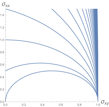
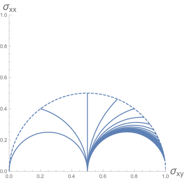
Figure 1: (Left) Phase diagram of the flow in the space of conductivities fills the fundamental domain of the upper half plane in units of $\hat{\sigma}=\rho/B$. Different curves correspond to different bare values $\zeta$ of $\sigma_{xx}$. The bare value of $\sigma_{xy}$ is set to zero ($W=0$). (Right) The flow diagram of the theory upon the $STS$ transformation.

The phase diagram makes explicit the full duality structure of the theory. From [3] (page 2), note that for Abelian CS theories the T operation of $Sl(2,\mathbb{Z})$ acts as $\theta\rightarrow\theta+2\pi$, which means in our notation $W(r_{h})\rightarrow W(r_{h})+\hat{\sigma}/4$. Such shift simply translates the diagram on figure 1 to the next copy of the fundamental domain. Moreover, from eq. 4.6 in [3], from the current-current correlator in momentum space, from the $\delta_{ij}k^{2}-k_{i}k_{j}$ and the $\epsilon_{ijk}$ components, with coefficients $t$ and $w$, one creates $\tau=w+it$, on which S acts as $\tau\rightarrow-1/\tau$, and T acts as $w\rightarrow w+1$, as in the terms in the action above. Note that this is morally (if not rigorously) related to the action on the conductivity, since by the Kubo relation the conductivity is the retarded current-current correlator in momentum space, divided by $i\omega$.

Note that here, in the context of theories with holographic dual, the duality group is expected to be $Sl(2,\mathbb{Z})$ instead of $Sl(2,\mathbb{R})$, the reason being that in the holographic dual the corresponding electromagnetic black holes have integer charges $Q_{e}$ and $Q_{m}$.

Modular transformations map a point in the fundamental domain to an infinite set of dual theories (dual sets of values of the parameters). This action can also be understood as action on sets of initial conditions in the RG flow. At $W=0$ S-duality inverts the initial values of the RG flow (points on the vertical axis). Inside the fundamental domain the corresponding flows exchange accordingly. Indeed, equations (3.6) transform as (3.34) provided (3.39) and $Z/g_{4}^{2}\to g_{4}^{2}/Z$. T transformations, as said before, translate the flow horizontally between the neighboring domains.

For $W\neq 0$, transformations (3.39) and (3.41) no longer act on the conductivities as the S transformation of $Sl(2,\mathbb{Z})$. However, they still act properly on the initial values of the flow. An example of the flow generated by an $STS$ transformation of the initial conditions and of the flow equations (3.45) is shown on the right plot of figure 1. It is not fully surprising that for a general copy of the domain, the S transformation is not defined in the same way as in the original domain at $W=0$. One can note that the difference with the $W=0$ transformation in this case, is that S transformation is not expected to act within the domain. The role of the latter transformation is played by $T^{w}ST^{-w}$.

The next question is whether we can have an action of this $Sl(2,\mathbb{Z})$ on heat conductivity, and correspondingly on the Wiedemann-Franz law as well.

In the 2+1 dimensional field theory, a self-duality of transport coefficients in $W=\Phi=0$ theory was noted in [8] (there it also extended to the AC coefficients). The transport coefficients of their model were (note that we should actually replace $\omega\rightarrow\omega+i/\tau_{\rm imp}$, were $\tau_{\rm imp}$ is the average time of scattering on impurities)

$$\sigma_{xx}=\sigma_{Q}\frac{\omega(\omega+i\gamma+i\omega_{c}^{2}/\gamma)}{[(\omega+i\gamma)^{2}-\omega_{c}^{2}]}\,, \sigma_{xy}=-\frac{\rho}{B}\frac{\gamma^{2}+\omega_{c}^{2}-2i\gamma\omega}{[(\omega+i\gamma)^{2}-\omega_{c}^{2}]}\,,$$ (3.47)

$$\rho_{xx}=\frac{1}{\sigma_{Q}}\frac{\omega(\omega+i\omega_{c}^{2}/\gamma+i\gamma)}{[(\omega+i\gamma)^{2}-\omega_{c}^{2}]}\,, \rho_{xy}=\frac{B}{\rho}\frac{(\omega_{c}^{2}/\gamma)^{2}+\omega_{c}^{2}-2i(\omega_{c}^{2}/\gamma)\omega}{[(\omega+i\gamma)^{2}-\omega_{c}^{2}]}\,,$$ (3.48)

$$\alpha_{xx}=\frac{\rho}{T}\frac{i\omega}{(\omega+i\gamma)^{2}-\omega_{c}^{2}}\,, \alpha_{xy}=-\frac{s}{B}\frac{\gamma^{2}+\omega_{c}^{2}-i\gamma\omega}{(\omega+i\gamma)^{2}-\omega_{c}^{2}}\,,$$ (3.49)

$$\theta_{xy}=-\frac{B}{T}\frac{i\omega}{(\omega+i\omega_{c}^{2}/\gamma)^{2}-\omega_{c}^{2}}\,, \theta_{xx}=\frac{s}{\rho}\frac{(\omega_{c}^{2}/\gamma)^{2}+\omega_{c}^{2}-i(\omega_{c}^{2}/\gamma)\omega}{(\omega+i\omega_{c}^{2}/\gamma)^{2}-\omega_{c}^{2}}\,,$$ (3.50)

$$\bar{\kappa}_{xx}=s\frac{i\omega-\gamma}{(\omega+i\gamma)^{2}-\omega_{c}^{2}}\,, \bar{\kappa}_{xy}=-s\frac{\omega_{c}}{(\omega+i\gamma)^{2}-\omega_{c}^{2}}\,,$$ (3.51)

$$\kappa_{xx}=s\frac{i\omega-\omega_{c}^{2}/\gamma}{(\omega+i\omega_{c}^{2}/\gamma)^{2}-\omega_{c}^{2}}\,, \kappa_{xy}=s\frac{\omega_{c}}{(\omega+i\omega_{c}^{2}/\gamma)-\omega_{c}^{2}}\;,$$ (3.52)

where $\sigma_{Q}$ is the electrical conductivity of the quantum critical system, $\omega_{c}$ has the interpretation as cyclotron frequency (and is indeed proportional to $eB$), and $\gamma$ is the damping frequency of the cyclotron modes.

The claim of [8] is that the transformations

$$\rho\leftrightarrow B\;,\qquad\sigma_{Q}\leftrightarrow\frac{1}{\sigma_{Q}}\;,\qquad\gamma\leftrightarrow\frac{\omega_{c}^{2}}{\gamma}$$ (3.53)

imply the following duality on the transport coefficients that comes from exchanging $E_{i}\leftrightarrow\epsilon_{ij}J_{j}$ (sources with response fields) in the transport equations,

$$\sigma_{xx}\rightarrow{\rho_{xx}} \sigma_{xy}\rightarrow-{\rho_{xy}}$$ (3.54)

$$\alpha_{xx}\rightarrow-\theta_{xy}=-(\hat{\sigma}^{-1}\hat{\alpha})_{xy} \alpha_{xy}\rightarrow-\theta_{xx}$$ (3.55)

$$\bar{\kappa}_{xx}\rightarrow\kappa_{xx} \bar{\kappa}_{xy}\rightarrow-\kappa_{xy}\;,$$ (3.56)

which includes an action on the heat conductivity. We remind the reader that the resistivities are defined as a matrix, inverse to the matrix of conductivities, $\hat{\rho}=\hat{\sigma}^{-1}$, which implies that

$$\rho_{xx}\ =\ \frac{\sigma_{xx}}{\sigma_{xx}^{2}+\sigma_{xy}^{2}}\,,\qquad\rho_{xy}\ =\ -\frac{\sigma_{xy}}{\sigma_{xx}^{2}+\sigma_{xy}^{2}}\,,$$ (3.57)

However, that is not quite consistent due to some signs. First, we see that, in order to have a duality, in fact we need to change

$$\sigma_{Q}\rightarrow\frac{1}{\sigma_{Q}}\;,\;\;\rho\rightarrow B\;,\;\;B\rightarrow-\rho\;,$$ (3.58)

(together with the same $\gamma\leftrightarrow\omega_{c}^{2}/\gamma$) which is consistent with our description of the S-duality. Second, we note that, for $\sigma_{ij}=\sigma_{xx}\delta_{ij}+\sigma_{xy}\epsilon_{ij}$, $E_{i}\rightarrow\epsilon_{ij}J_{j}$ results in $\rho_{il}\leftrightarrow\epsilon_{ij}\sigma_{jk}\epsilon_{kl}=-\sigma_{il}$, or $\rho_{xx}\leftrightarrow-\sigma_{xx}$, $\rho_{xy}\leftrightarrow-\sigma_{xy}$. On the other hand, $E_{i}\leftrightarrow J_{i}$ results in $\sigma_{ij}\leftrightarrow\rho_{ij}$, so we have in some sense half transformation from one duality, half from the other (but of course, that is not permitted). Finally, we note that in both cases, at $\alpha_{ij}=0$, we should have $\bar{\kappa}_{xy}\leftrightarrow\kappa_{xy}$, which is different than the above duality (3.56), where we have a minus sign.

One might think, why consider the formulas in [8], since they are for a model defined in 2+1 dimensions, and not holographically? The reason is that the results for the transport coefficients match exactly! First, the holographic formulas (3.6) and (3.10) (and even the thermoelectric ones, $\alpha_{xx}$ and $\alpha_{xy}$, in [9]) are for DC transport, so at $\omega=0$, but we said that really $\omega\rightarrow\omega+i/\tau_{\rm imp}$, so for matching we should replace $\omega$ with $i/\tau_{\rm imp}$, but the breaking of translational invariance due to impurities is replaced in our case by $\Phi$, which does the same. Then (assuming that the $\Phi$ term should be identified with the $1/\tau_{\rm imp}$ term) indeed, the formulas for electric conductivities are the same, if (and only if) we identify

$$\frac{1}{\tau_{\rm imp}\omega_{c}}=\frac{e^{2V}k^{2}\Phi}{2\kappa_{4}^{2}B\rho}\;,\;\;\;\frac{\gamma}{\omega_{c}}=\frac{BZ}{\rho g_{4}^{2}}$$ (3.59)

$$\sigma_{Q}=\frac{Z}{g_{4}^{2}}.$$ (3.60)

We can also identify the formula for $\bar{\kappa}_{xy}$, provided we have

$$\omega_{c}=\frac{\rho B}{sT}.$$ (3.61)

With these identifications (which already involved several nontrivial consistency checks), all other transport coefficients ($\bar{\kappa}_{xx},\alpha_{xx},\alpha_{xy}$) are also matched. Then finally, we have the identification of parameters

$$\sigma_{Q} = \frac{Z}{g_{4}^{2}}=\zeta$$ (3.62)

$$\omega_{c} = \frac{\rho B}{sT}=\frac{B^{2}}{sT}\hat{\sigma}$$ (3.63)

$$\frac{1}{\tau_{\rm imp}} = \frac{e^{2V}k^{2}\Phi}{2\kappa_{4}^{2}}\frac{1}{sT}=\frac{B^{2}}{sT}\lambda$$ (3.64)

$$\gamma = \frac{Z}{g_{4}^{2}}\frac{B^{2}}{sT}=\frac{B^{2}}{sT}\zeta\;,$$ (3.65)

where the second expressions are in terms of the reduced variables defined for the RG flow. We see that indeed, we had correctly identified the parameters, rescaled by $B^{2}/(sT)$, which is the factor that relates $\sigma_{Q}$ with $\gamma$. Second, $\lambda$, which is related to $\tau_{\rm imp}$ (the scale defined by impurities), was correctly described as an RG scale, while also $\sigma_{Q}=\zeta$, the electric conductivity of the quantum critical system, was correctly described as value in the UV point ($\lambda\rightarrow\infty$).

Then, given this match to the DC holographic formulas (3.6) and (3.10), we can extend them to the AC regime by replacing as in [8]

$$\lambda\frac{s}{\rho^{2}}=\frac{1}{\tau_{\rm imp}}\rightarrow\frac{1}{\tau_{\rm imp}}-i\omega.$$ (3.66)

In the above analysis we compared formulas (3.6)-(3.24), derived holographically in the approximation of weak electric and magnetic fields, with equations (3.49)-(3.52) derived hydrodynamically in the approximation of weak magnetic field. Consequently our values of $\omega_{c}$ and $\gamma$ match the hydrodynamic values of [8] in the approximation $\mu\ll T$. On the other hand, we will see that equations (3.6)-(3.24) are also valid in the case of the dyonic black hole solution, for any $B$ and $\rho$, so a small disagreement between the results remains.

More recently, the hydrodynamic derivation of the conductivities was generalized to arbitrary values of $B$ in [32]. Here, to match equations (3.49)-(3.52) we simply assumed that the frequency can be reinstated by a shift of $1/\tau_{\rm imp}$. The authors of [32] show that the correct $\omega$ dependence is captured by the higher order corrections in $B$, and that the hydrodynamic and holographic results match. It was also noted that conductivities, apart from $\sigma_{Q}$ also depend on another universal parameter $\sigma_{H}$ – the incoherent Hall conductivity. This is consistent with the picture discussed in this work, since the “flow” of the conductivities is two-dimensional, determined in terms of two initial values $\zeta$ and $w$.

As we saw in the example of Abelian CS of [3] there is a duality that acts on the parameters in the action, and a duality that acts in the resulting current-current correlators, or transport coefficients. In the first way of thinking $S$ and $T$ transformations act on parameters, with the functional form of the transport coefficients in terms of them constant (passive duality), while in the second way the parameters remain unchanged but $S$ and $T$ act on the transport coefficients themselves (active duality), and the result is the same.

We can construct a heat analog of the complex conductivity,

$$\frac{\bar{\kappa}}{T}\equiv\frac{\bar{\kappa}_{xy}+i\bar{\kappa}_{xx}}{T}=\frac{s^{2}}{B}\frac{\rho+i\left(\frac{BZ}{g_{4}^{2}}+\frac{e^{2V}k^{2}\Phi}{(2\kappa_{4}^{2})B}\right)}{\rho^{2}+\left(\frac{BZ}{g_{4}^{2}}+\frac{e^{2V}k^{2}\Phi}{(2\kappa_{4}^{2})B}\right)^{2}}=\frac{s^{2}}{B}\frac{1}{\rho-i\left(\frac{BZ}{g_{4}^{2}}+\frac{e^{2V}k^{2}\Phi}{(2\kappa_{4}^{2})B}\right)}.$$ (3.67)

Then the S-duality acts on it as

$$\frac{\bar{\kappa}}{T}\rightarrow-\frac{s^{2}}{\rho}\frac{1}{B+i\left(\rho\frac{g_{4}^{2}}{Z}+\frac{e^{2V}k^{2}\Phi}{(2\kappa_{4}^{2})\rho}\right)}=i\frac{B}{\rho}\frac{Z}{g_{4}^{2}}\frac{s^{2}}{B}\frac{1}{\rho-i\frac{Z}{g_{4}^{2}}B+\frac{Ze^{2V}k^{2}\Phi}{(2\kappa_{4}^{2})g_{4}^{2}\rho}}.$$ (3.68)

So, while $\kappa/T$ looks nice even for nonzero $\Phi$, the transformation looks understandable as an active transformation only at $\Phi=0$, or if

$$\Phi\rightarrow-i\frac{\rho}{B}\frac{g_{4}^{2}}{Z}\Phi$$ (3.69)

Then,

$$\bar{\kappa}\ \rightarrow\ i\frac{B}{\rho}\frac{Z}{g_{4}^{2}}\bar{\kappa}\,,$$ (3.70)

which amounts to

$$\bar{\kappa}_{xx}\ \to\ -\frac{Z}{g_{4}^{2}}\frac{\bar{\kappa}_{xy}}{\sigma_{xy}}\,,\qquad\bar{\kappa}_{xy}\ \to\ \frac{Z}{g_{4}^{2}}\frac{\bar{\kappa}_{xx}}{\sigma_{xy}}\,.$$ (3.71)

This can be understood as a simple S-duality action on real ratios (rather than the complex combination $\kappa$ defined above)

$$\frac{\bar{\kappa}_{xx}}{{\bar{\kappa}}_{xy}}\ \to\ -\frac{{\bar{\kappa}}_{xy}}{\bar{\kappa}_{xx}}\,.$$ (3.72)

In fact, from the point of view of self-duality (3.56) observed in [8], it is more natural to think of the duality transformation as action exchanging $\kappa$ with $\bar{\kappa}$ which is also an action on the real ratios, or as $2\times 2$ matrix action,

$$\frac{\kappa_{xx}}{\bar{\kappa}_{xx}}\ \to\ \frac{\bar{\kappa}_{xx}}{\kappa_{xx}}\,,\qquad\frac{\kappa_{xy}}{\bar{\kappa}_{xy}}\ \to\ \frac{\bar{\kappa}_{xy}}{\kappa_{xy}}\,.$$ (3.73)

We remind the reader that $\bar{\kappa}$ and ${\kappa}$ are heat and thermal conductivities (the difference between them, expressed by equation (2.2), is that the contribution to heat transport from electric fields must be subtracted from the latter). One can observe the simple duality $\bar{\kappa}_{ij}\leftrightarrow\kappa_{ij}$ directly in equations (3.24), for any $\Phi$.

Finally we note again that for $W\neq 0$ the S-duality transformation makes sense only if $W(r_{h})=n2\pi$. In this case, even including $\Phi$, the transformation above can be understood (instead of just S-duality) as a passive transformation of $ST^{n}$, where $T^{n}$ ($n$ T operations $W\rightarrow W+2\pi$) cancels out $W$, and $\Phi(r_{h})$ is included as a parameter, as well as $e^{2V(r_{h})}$, and are unchanged under the dualities.

It is also interesting to check the action of duality in the low temperature limit of the conductivities.

$$\bar{\kappa}_{xx}\ \to\ \bar{\kappa}_{xx}=\frac{\pi^{2}}{3}cT\,,\qquad\bar{\kappa}_{xy}\ =\ \frac{\pi^{2}}{3}c\frac{{g_{4}}^{2}}{Z}\sigma_{xy}T\ \to\ \kappa^{\prime}_{xy}=\frac{\pi^{2}}{3}c\frac{{g_{4}^{\prime}}^{2}}{Z^{\prime}}\sigma^{\prime}_{xy}T\,,$$ (3.74)

where

$$\sigma^{\prime}_{xy}=-\frac{B}{\rho}=-\frac{1}{\sigma_{xy}}\,,\qquad\frac{Z^{\prime}}{{g_{4}^{\prime}}^{2}}=\frac{g_{4}^{2}}{Z}\,.$$ (3.75)

We see that the direct heat conductivity is invariant under the action of S-duality, which agrees with the above observation that $\bar{\kappa}_{xx}=\kappa_{xx}$ in the $\Phi=0$ limit. It also agrees with the non-electron (phonon) origin of the direct heat transport at low temperatures. On the other hand, the Leduc-Righi (transverse) conductivity is transformed in accordance with the particle-vortex picture.

The action of S-duality, corresponding (modulo signs) to the exchange $E_{i}\leftrightarrow\epsilon_{ij}J_{j}$, namely $\sigma_{xy}\rightarrow 1/\sigma_{xy}$ for $\sigma_{xx}\simeq 0$, $\bar{\kappa}_{xx}\rightarrow\kappa_{xx}$, $\bar{\kappa}_{xy}\rightarrow-\kappa_{xy}$, explains the exchange of the modified (transverse) Lorenz number $\bar{L}$ with the usual one $L$ only with a given dependence on $c$ for the case $cg_{4}^{2}=\pi Z$, namely if

$$\frac{\bar{\kappa}_{xy}}{T}=\frac{\pi cg_{4}^{2}}{3Z}\sigma_{xy}\Rightarrow\bar{L}=\frac{\bar{\kappa}_{xy}}{T\sigma_{xy}}=\frac{\pi^{2}}{3}\;,$$ (3.76)

as we obtained, being mapped by S-duality into

$$-\frac{\kappa_{xy}}{T}=\frac{\pi c}{3}\frac{Z}{g_{4}^{2}}\frac{1}{\sigma_{xy}}\Rightarrow L=\frac{\kappa_{xy}}{T\sigma_{xy}}=-\frac{c^{2}}{3\sigma^{2}_{xy}}\;,$$ (3.77)

where in the last equality we have used again $cg_{4}^{2}=\pi Z$.

3.3 Wiedemann-Franz law from the dyonic black hole dual

In this subsection, we will see that we indeed obtain the correct generalized Wiedemann-Franz law expected from the previous section, and calculate some interesting relations between thermodynamical quantities and conductivites.

We will first summarize the calculations of the conductivities in [7, 8], using their notation, which implicitly assumes $cg_{4}^{2}=\pi Z$, and then generalize to the case of the two parameters being independent. Assuming for simplicity $Z=1$, we see that in those works $1/g_{4}^{2}=1/(4\pi G_{N})$ and radius $R=1$, which gives the central charge as $c=R^{2}/(4G_{N})=\pi/g_{4}^{2}$. We can see that by comparing their action,

$$S=\left(\frac{\sqrt{2}N^{3/2}}{6\pi}\right)\int d^{4}x\sqrt{-g}\left[-\frac{R}{4}+\frac{F_{\mu\nu}^{2}}{4}-\frac{3}{2}+...\right]$$ (3.78)

with our (canonical) form of the action,

$$S=\int d^{4}x\sqrt{-g}\left[\frac{R}{16\pi G_{N}}-\frac{F_{\mu\nu}^{2}}{4g_{4}^{2}}-\frac{6}{R^{2}}+...\right].$$ (3.79)

We also note that their $G_{N}$ is dimensionless and a function of only $N$.

The dyonic black hole in [7, 8] is given by the metric

$$ds^{2}\ =\ \frac{\alpha^{2}}{z^{2}}\left(-f(z)dt^{2}+dx^{2}+dy^{2}\right)+\frac{1}{z^{2}}\frac{dz^{2}}{f(z)}\,,$$ (3.80)

where

$$f(z)\ =\ 1+(h^{2}+q^{2})z^{4}-(1+h^{2}+q^{2})z^{3}\,,$$ (3.81)

and the Maxwell field tensor is

$$F\ =\ h\alpha^{2}dx\wedge dy+q\alpha dz\wedge dt\,.$$ (3.82)

Note that the horizon radius is $z=1$, but there is a parameter $\alpha$, which has a role similar to the inverse horizon radius. Identifying the chemical potential with the asymptotic value of the temporal component of the gauge potential and demanding that the component vanishes at the horizon gives

$$\mu=-q\alpha\,.$$ (3.83)

The magnetic field is given by the flux of $F$ through the $xy$ plane, $B=h\alpha^{2}$.

The Bekenstein-Hawking temperature of the black hole is determined through the relation

$$\frac{4\pi T}{\alpha}\ =\ 3-\frac{\mu^{2}}{\alpha^{2}}-\frac{B^{2}}{\alpha^{4}}\,.$$ (3.84)

Computing the Euclidean action on the black hole solution and equating it to the thermodynamic potential, one gets, after subtracting appropriate counterterms [8],

$$\frac{\Omega}{V}\ =\ c\frac{\alpha^{3}}{4\pi}\left(-1-\frac{\mu^{2}}{\alpha^{2}}+3\frac{B^{2}}{\alpha^{4}}\right)\,.$$ (3.85)

From this expression one can compute the entropy density,

$$s=\frac{S}{V}\ =\ -\left.\frac{1}{V}\frac{\partial\Omega}{\partial T}\right|_{B,\mu}\ =\ c\alpha^{2}\,,$$ (3.86)

where we obtain $T=T(\alpha,B,\mu)$ from (3.84) in order to calculate the partial derivative of $\Omega(T,\mu,B)$ at fixed $T$ and $\mu$, and the charge density

$$\rho\ =\ -\frac{1}{V}\left.\frac{\partial\Omega}{\partial\mu}\right|_{B,T}\ =\ \frac{c}{\pi}\alpha\mu\;,$$ (3.87)

where we do the same.

We are also interested in the second derivatives of the potential, giving the susceptibilities. One can similarly compute those derivatives, where after similarly using $T(\alpha,B,\mu)$ in the derivatives, we put $T\simeq 0$ in (3.84), to find

$$-\frac{1}{V}\left.\frac{\partial^{2}\Omega}{\partial\mu^{2}}\right|_{B,T}\ =\ \frac{6c\alpha_{0}^{3}/\pi}{6\alpha_{0}^{2}-\mu^{2}}+O(T)\,,$$ (3.88)

and

$$-\frac{T}{V}\left.\frac{\partial^{2}\Omega}{\partial T^{2}}\right|_{B,\mu}\ =\ \frac{4c\pi\alpha_{0}^{3}}{6\alpha_{0}^{2}-\mu^{2}}T+O(T^{2})\,,$$ (3.89)

where we only evaluated the lowest order contribution at low temperature. The zero temperature value $\alpha_{0}$ is fixed from equation (3.84).

The above two susceptibilities are the diagonal entries of the complete susceptibility matrix. We can also compute similarly the off-diagonal entries, to find the matrix

$$\chi_{s}\ =\ \left(\begin{array}[]{cc}\frac{6c\alpha_{0}^{3}/\pi}{6\alpha_{0}^{2}-\mu^{2}}&\frac{2c\mu\alpha_{0}^{2}}{6\alpha_{0}^{2}-\mu^{2}}\\ \frac{2c\mu\alpha_{0}^{2}}{6\alpha_{0}^{2}-\mu^{2}}T&\frac{4c\pi\alpha_{0}^{3}}{6\alpha_{0}^{2}-\mu^{2}}T\end{array}\right)\;.$$ (3.90)

According to the general response theory in the hydrodynamic limit [14], the susceptibility matrix is related to the matrix of conductivities through relation (2.11), where $D$ is the matrix of diffusivities. Normally, in a field theory, like for instance the SYK case in [13], or the generic model used in [7], one calculates the dynamic susceptibilities $\chi(k,\omega)$ from 2-point functions of fluctuations in the model, and relating them with the static $\chi_{s}$ obtained from thermodynamics as above allows us to extract the diffusivity matrix $D$, and thus the conductivity matrix is found as $D\cdot\chi_{s}$.

However, in the holographic system of the dyonic black holes in [7, 8] analyzed above, like in a different holographic model (with some translational invariance induced by some linear axions) in [13], the holographic conductivities $\sigma_{ab},\alpha_{ab},\bar{\kappa}_{ab}$ are directly found, from the holographic retarded Green’s functions $G^{R}_{J_{a}J_{b}},G^{R}_{J_{a}\pi_{b}},G^{R}_{\pi_{a}\pi_{b}}$, respectively, by use of the Kubo formulas, or from calculations at the horizon (using the membrane paradigm). Then one conversely uses (2.11) to find the diffusivity matrix $D$ from the conductivity matrix and the static susceptibility matrix $\chi_{s}$. This is what we want to do as well.

In subsection 3.1 we considered the calculation of the conductivity matrix from a certain holographic model, which, like explained for instance in Appendix I of [13], is a priori different than the dyonic black hole model, so for consistency we should only use the formulas derived from it in [8]. The dyonic black hole has no translational invariance breaking, so one obtains $\sigma_{xx}=0$, and from $G^{R}_{J_{i}J_{j}}$ the classical Hall electric conductivity, $\sigma_{ij}=\frac{\rho}{B}\epsilon_{ij}$, consistent with the results in subsection 3.1 at $\Phi=0$. Yet for the other conductivities, the usual Kubo formulas do not apply anymore at $B\neq 0$ [7], but are modified according to [8],

$$\alpha_{ij} = \frac{1}{T}\frac{G^{R}_{J_{i}Q_{j}}}{i\omega}+\frac{M}{T}\epsilon_{ij}$$ (3.91)

$$\frac{\kappa_{ij}}{T} = \frac{1}{T}\frac{G^{R}_{Q_{i}Q_{j}}}{i\omega}+\frac{2(M_{E}-\mu M)}{T}\epsilon_{ij}.$$ (3.92)

We obtain relations compatible with the ones obtained in [9], but in the $\Phi\rightarrow 0$ limit, with $\bar{\kappa}_{ij}$ from (3.10) and $\alpha_{ij}$ from (3.14)

Together, we have for $\Phi=0$

$$\alpha_{ij}=\frac{s}{B}\epsilon_{ij}\;,\;\;\;\sigma_{ij}=\frac{\rho}{B}\epsilon_{ij}.$$ (3.93)

Also, from (3.10) for $\Phi=0$, we obtain

$$\frac{\bar{\kappa}_{xx}}{T} = \frac{s^{2}}{\rho^{2}}\frac{\frac{Z}{g_{4}^{2}}}{1+\frac{B^{2}}{\rho^{2}}\frac{Z^{2}}{g_{4}^{4}}}$$ (3.94)

$$\frac{\bar{\kappa}_{xy}}{T} = \frac{s^{2}}{\rho B}\frac{1}{1+\frac{B^{2}}{\rho^{2}}\frac{Z^{2}}{g_{4}^{4}}}\;,$$ (3.95)

the same result as derived from (3.92).

Given the fact that we used different ansätze for a starting point, and the results were only valid at $\Phi=0$, we should stop with the analysis of the dyonic black hole here.

However, we will for the moment assume (which is by no means obvious) that we can consider the dyonic black hole as a limit of the analysis of subsection 3.1, and use the formulas obtained there, combining them with ones derived in this subsection for the dyonic black hole.

In the holographic system of [13], which is different than our case but the logic can be imported, as it relies only on general properties of transport and thermodynamics, it was found that the diffusivity matrix has the structure given by equation (2.10), with

$$2\pi{\cal E}\ \equiv\ \left(\frac{\partial S}{\partial\rho}\right)_{T}\ =\ -\left(\frac{\partial\mu}{\partial T}\right)_{\rho}\ =\ \frac{4\pi^{2}}{3}\frac{c\alpha^{2}\rho}{c^{2}\alpha^{4}+B^{2}c^{2}+\pi^{2}\rho^{2}}.$$ (3.96)

The same structure of matrix $D$ was claimed to be reproduced by a multi-dimensional SYK model. Moreover, the equilibrium parameter ${\cal E}$ is directly related to the Seebeck coefficient,

$${\bar{S}}\ =\ \alpha\cdot\sigma^{-1}\ =\ 2\pi{\cal E}\,.$$ (3.97)

a nontrivial result, which however is claimed in [13] to be equivalent to the form (2.10) of the diffusivities matrix, at least in the $T\to 0$ limit. We will now discuss the structure of the transport of the dyonic black hole, with the stated caveat that we assume it arises as a limit of the general analysis in section 3.1 in this limit.

The conductivities in this $cg_{4}^{2}/Z=\pi$ convention, from [8], (or calculated from equations (3.6) and (3.10) with $W=0$ and $\Phi=0$, if we replace $g_{4}^{2}/Z$ with $\pi/c$) are

$$\sigma_{xy} = \frac{\rho}{B}\,,$$ (3.98)

$$\bar{\kappa}_{xy} = \sigma_{xy}\frac{\pi^{2}s^{2}T}{\pi^{2}\rho^{2}+c^{2}B^{2}}\,.$$ (3.99)

Taking the ratio of the conductivities and computing the lowest order contribution at $T\to 0$ by replacing $s$ in (3.86) and $\rho$ in (3.87) into the above, and using (3.84) in the limit $T\rightarrow 0$, one finds the modified Lorenz number (note that we use $\bar{\kappa}_{xy}$ instead of $\kappa_{xy}$ as we should have, as we already noted in section 3.1)

$$\bar{L}=\frac{\bar{\kappa}_{xy}}{\sigma_{xy}T}\ =\ \frac{\pi^{2}s^{2}}{\pi^{2}\rho^{2}+c^{2}B^{2}}\ =\ \frac{\pi^{2}}{3}+O(T)\,.$$ (3.100)

We can also recall equation (3.17) for the modified Lorenz number in the direct channel in the limit of zero magnetic field. For pure a system ($\Phi$=0) $L_{xx}$ is given by the same number: by a similar calculation, we find

$$\bar{L}_{xx}\xrightarrow{B,\Phi\to 0}\frac{s^{2}}{\rho^{2}}\ =\ \frac{\pi^{2}}{3}+O(T)\,.$$ (3.101)

The explanation of taking these modified Lorenz numbers $\bar{L}$ and $\bar{L}_{xx}$, and obtaining the free result is that, as we saw in the previous subsection, S-duality or particle-vortex duality exchanges (modulo some signs) $\kappa_{xy}$ with $\bar{\kappa}_{xy}$ and $\kappa_{xx}$ with $\bar{\kappa}_{xx}$, so we obtain the free result by using $\bar{\kappa}_{xy}$ and $\bar{\kappa}_{xx}$, which means basically that this strongly coupled calculation (as holographic dual to a perturbative gravity one) is S-dual to a free (or perturbative) system.

The diffusivity matrix $D$ is computed by inverting the relation (2.11). Since we are dealing with a system with both electric and magnetic fields, we will consider both the conductivity and the diffusivity matrices to be complex, $\sigma=\sigma_{xy}+i\sigma_{xx}$ and $D=D_{xy}+iD_{xx}$, as described in (2.12). For the imaginary part, which corresponds to the longitudinal ($xx$) conductivities, at any $T$,

$$D^{\parallel}\ =\ \left(\begin{array}[]{cc}0&0\\ -2\pi{\cal E}D_{2}^{\parallel}&D_{2}^{\parallel}\end{array}\right),\qquad D_{2}^{\parallel}\ =\ \frac{3}{8}\frac{c^{2}\alpha^{4}+B^{2}c^{2}+\pi^{2}\rho^{2}}{\alpha(B^{2}c^{2}+\pi^{2}\rho^{2})}.$$ (3.102)

Note that this equation trivially implies $\sigma_{xx}=0$ and $\alpha_{xx}=0$, which is consistent with the above relations. But since $T\alpha_{xx}=0$, the lower left corner of the $D\chi_{s}$ matrix needs to vanish as well, and it does, since we can check that

$$D_{2}^{\parallel}(-2\pi{\cal E}\chi_{11}+\chi_{21})=0.$$ (3.103)

This seems nontrivial, but note that both $2\pi{\cal E}$ and $\chi_{ij}$ are calculated as thermodynamical coefficients. In fact,

$$\chi_{11}=-\left.\frac{\partial^{2}\Omega}{V\partial\mu^{2}}\right|_{B,T}=\left.\frac{\partial\rho}{\partial\mu}\right|_{B,T}\;,\;\;\;\chi_{21}=-\left.\frac{\partial}{\partial\mu}\left.\left(\frac{\partial\Omega}{V\partial\mu}\right|_{B,\mu}\right)\right|_{B,T}=\left(\frac{\partial S}{\partial\mu}\right)_{B,T}\;,$$ (3.104)

so the identity is actually

$$\left(\frac{\partial S}{\partial\mu}\right)_{B,T}=\left(\frac{\partial S}{\partial\rho}\right)_{B,T}\left(\frac{\partial\rho}{\partial\mu}\right)_{B,T}\;,$$ (3.105)

which is correct.

The form of $D^{\parallel}$ in (3.102) is the form of the matrix (2.10), found in [13] to be obtained also in the SYK model, for $D_{1}=0$. Indeed, in a clean, $\Phi=0$, gapped, $B\neq 0$, system one does not expect charge diffusion.

One also has a real component of the diffusion in this system, defined by the transverse ($xy$) transport,

$$D^{\perp}\ =\ \left(\begin{array}[]{cc}\frac{\pi\rho}{2c\alpha B}&\frac{3c^{2}\alpha^{4}+3B^{2}c^{2}-\pi^{2}\rho^{2}}{8\pi c^{2}\alpha^{3}BT}\\ \frac{\pi\alpha T(2B^{2}c^{2}+\pi^{2}\rho^{2})}{2B(B^{2}c^{2}+\pi^{2}\rho^{2})}&\frac{\pi\rho(3c^{2}\alpha^{4}-B^{2}c^{2}-\pi^{2}\rho^{2})}{8c\alpha B(B^{2}c^{2}+\pi^{2}\rho^{2})}\end{array}\right)\,.$$ (3.106)

It is not of the form (2.10).

Finally, from (3.93) in the $B\rightarrow 0$ limit, for the clean system at $\Phi=0$, the Seebeck coefficient is simply [25]

$$\bar{S}_{ab}\ =\ \frac{s}{\rho}\,\delta_{ab}\ =\ \frac{\pi}{\sqrt{3}}\delta_{ab}+O(T)\,.$$ (3.107)

The $T\to 0$ limit, for $B\rightarrow 0$ also, indeed agrees with the value of $2\pi{\cal E}$ in (3.97), as conjectured in [13]. Yet it is puzzling that in this case we have $S=2\pi{\cal E}$, but no $D$ of the form (2.10), when in [13] they were claimed to be equivalent. We leave a full understanding of this fact for later.

We also add that the ${\cal O}(T)$ coefficient in $S_{ab}$ satisfies the so called Mott relation [25].

Equations (3.100) and (3.101) precisely reproduce the canonical (weak coupling) Lorenz number from a holographic calculation. This was previously observed in [24] and further elaborated in [25].

However, we note that, first, this result is obtained for a specific normalization of coupling constants, and, second, the Lorenz number was computed for the coefficient $\bar{\kappa}$, while the canonical one uses the thermal conductivity $\kappa$ (2.2), as noted above.

Since S-duality exchanges $\kappa_{xx}\to\bar{\kappa}_{xx}$ at low temperatures, the transverse conductivities yield the (unmodified) Lorenz number

$$L\ =\ \frac{\kappa}{\sigma T}\ =\ \frac{c^{2}}{3\sigma^{2}}+O(T)\,,$$ (3.108)

in this limit. We have already noted in the previous subsections that this is just S-dual to the free value for the modified Lorenz number. Let us discuss these issues in more detail.

The particular normalization used in [7, 8] arises from a holographic model obtained by considering a consistent truncation of the low-energy limit of M theory on $AdS_{4}\times S^{7}$[12, 33]. This model flows to a superconformal fixed point in the IR, which is known as the ABJM model [34]. Hence it describes a universality class of $2+1$ dimensional systems. We will see however, that relation (3.100) is not preserved by the duality. More generally, the Lorenz number will depend on $g_{4}^{2}$.

For independent $g_{4}$ and $c$, the above equations generalize as follows. From (3.78) we see that in order to go to the canonical form with independent $c$ and $g_{4}^{2}$, we need to write $(A_{\mu})^{2}=(\tilde{A}_{\mu})^{2}\frac{Z}{g_{4}^{2}}\frac{\pi}{c}$, so $B^{2}=\tilde{B}^{2}\frac{Z}{g_{4}^{2}}\frac{\pi}{c}$ and $\mu^{2}=\tilde{\mu}^{2}\frac{Z}{g_{4}^{2}}\frac{\pi}{c}$.

Then the blackening factor of the black metric and the temperature generalize to

$$f(z)\ =\ 1-\left(1+\frac{Z\pi}{cg_{4}^{2}}\left(\frac{\mu^{2}}{\alpha^{2}}+\frac{B^{2}}{\alpha^{4}}\right)\right)z^{3}+\frac{Z\pi}{cg_{4}^{2}}\left(\frac{\mu^{2}}{\alpha^{2}}\frac{B^{2}}{\alpha^{4}}\right)z^{4}$$ (3.109)

and

$$\frac{4\pi T}{\alpha}\ =\ 3-\frac{Z\pi}{cg_{4}^{2}}\left(\frac{\mu^{2}}{\alpha^{2}}+\frac{B^{2}}{\alpha^{4}}\right).$$ (3.110)

The expression for the thermodynamics potential becomes

$$\frac{\Omega}{V}\ =\ \frac{c\alpha^{3}}{4\pi}\left(-1+\frac{Z\pi}{cg_{4}^{2}}\left(-\frac{\mu^{2}}{\alpha^{2}}+3\frac{B^{2}}{\alpha^{4}}\right)\right).$$ (3.111)

The expression for the entropy remains unmodified but a factor of $g_{4}^{2}$ is restored in the charge density,

$$s = c\alpha^{2}\,,$$ (3.112)

$$\rho = \frac{Z\mu\alpha}{g_{4}^{2}}\,.$$ (3.113)

For the second derivatives (the susceptibilities) the result is

$$-\frac{1}{V}\frac{\partial^{2}\Omega}{\partial\mu^{2}} = \frac{3\alpha Z\left(1+\frac{\pi Z}{cg_{4}^{2}}\left(\frac{\mu^{2}}{\alpha^{2}}+\frac{B^{2}}{\alpha^{4}}\right)\right)}{g_{4}^{2}\left(3+\frac{\pi Z}{cg_{4}^{2}}\left(\frac{\mu^{2}}{\alpha^{2}}+3\frac{B^{2}}{\alpha^{4}}\right)\right)}\ \to\ \frac{6\alpha^{3}Z}{g_{4}^{2}\left(6\alpha^{2}-\frac{\pi Z\mu_{0}^{2}}{cg_{4}^{2}}\right)}\,,$$ (3.114)

$$-\frac{T}{V}\frac{\partial^{2}\Omega}{\partial T^{2}} = \frac{2\alpha^{2}c\left(3-\frac{\pi Z}{cg_{4}^{2}}\left(\frac{\mu^{2}}{\alpha^{2}}+\frac{B^{2}}{\alpha^{4}}\right)\right)}{\left(3+\frac{\pi Z}{cg_{4}^{2}}\left(\frac{\mu^{2}}{\alpha^{2}}+3\frac{B^{2}}{\alpha^{4}}\right)\right)}\ \to\ \frac{4c\pi\alpha^{3}T}{\left(6\alpha^{2}-\frac{\pi Z\mu_{0}^{2}}{cg_{4}^{2}}\right)}\,,$$ (3.115)

$$-\frac{T}{V}\frac{\partial^{2}\Omega}{\partial\mu\partial T} = \frac{4\pi Z\mu T}{g_{4}^{2}\left(3+\frac{\pi Z}{cg_{4}^{2}}\left(\frac{\mu^{2}}{\alpha^{2}}+3\frac{B^{2}}{\alpha^{4}}\right)\right)}\ \to\ \frac{2\pi Z\alpha^{2}\mu_{0}T}{g_{4}^{2}\left(6\alpha^{2}-\frac{\pi Z\mu_{0}^{2}}{cg_{4}^{2}}\right)}\,.$$ (3.116)

We now consider the expressions (3.10) and (3.6) for the conductivities, with $\Phi=W=0$, and obtain

$$\bar{L}\ =\ \frac{s^{2}}{\rho^{2}+\frac{ZB^{2}}{g_{4}^{4}}}\ =\ \frac{c^{2}\alpha^{4}}{\frac{Z^{2}}{g_{4}^{4}}\left(\frac{\mu^{2}}{\alpha^{2}}+\frac{ZB^{2}}{\alpha^{4}}\right)\alpha^{4}}\ =\ \frac{(cg_{4}^{2})^{2}}{Z^{2}(q^{2}+h^{2})}\;,$$ (3.117)

but from (3.110), we get that, as $T\rightarrow 0$, now $q^{2}+h^{2}=3cg_{4}^{2}/\pi Z$, so we obtain

$${\bar{L}}\ =\ \frac{\pi}{3}\frac{cg_{4}^{2}}{Z}\,.$$ (3.118)

which is not quite the expected universal number. Under S-duality it is transformed as

$${\bar{L}}\to\frac{\pi}{3}\frac{cZ}{g_{4}^{2}}\,,$$ (3.119)

so even in the special case of the the top-down theory on M2 branes (ABJM), ${\bar{L}}$ is transformed into a “strong coupling” value with a structure less resembling equation (2.14).

However, we note that $g_{4}$, in the M2 brane normalization, is the coupling of the gravity theory, so the strong coupling regime is in fact a weak coupling regime of the dual gauge theory. We cannot, in general, expect gravity results to be valid for large $g_{4}$. However, we can expect the duality to hold and act on the conductivities as discussed in the previous section. Consequently, the duality exchanges the values of $\bar{\kappa}_{xy}$ and $\kappa_{xy}$, so in the weakly coupled gauge theory the value of the canonical Lorenz number $L$ is as it should be, provided by equation (3.100).

In summary, the following picture emerges. In the theory dual to the low-energy limit of M2 branes the weak coupling value of the electron Lorenz number is given by its canonical value $\pi^{2}/3$. When electron interactions are not negligible, the Lorenz number is modified. In the strong coupling limit, $\kappa_{xy}$ is inversely proportional to $\sigma_{xy}$, with the coefficient $c^{2}/3$. In the meantime the dual vortex Lorenz number has the canonical value at strong coupling, where weakly interacting vortices replace electrons. Duality exchanges the values of the electron and vortex Lorenz numbers when going from weak to strong coupling. The M2 brane values do not appear universal and might be modified once a different gauge theory dual to the dyonic black hole is constructed.

Finally, we comment on the question we put before about the fact that at fixed $g_{4}^{2}$, since we have $s^{2}\propto c^{2}$, we expected $L\propto c^{2}$, because we understood $\rho$ and $B$ as being applied fields in the boundary theory and $g_{4}^{2}$ as a parameter. If we derive them from the gravity dual in terms of given $q$ and $h$, and take $T\rightarrow 0$, then it seems that indeed, we get the right answer, but why do that? We need to assume that

$$\rho^{2}+\frac{B^{2}}{g_{4}^{4}}=\frac{3c}{\pi}\alpha^{4}\frac{Z}{g_{4}^{2}}\propto c\;,$$ (3.120)

for fixed $\alpha$ and $g_{4}^{2}$. The answer we believe is, as already hinted, that $Z\equiv Z(r_{H})$ is the horizon value of a field, which corresponds to a variation of the field theory on the boundary, allowing the dependence on $c$ of the denominator.

4 Transport coefficients from one dimensional effective action for AdS/CMT holographic dual

4.1 One dimensional effective action for transport in holographic models and extensions of SYK

In [13, 35], an effective action has been proposed that includes charge in the SYK model, making it a model of complex fermions, and in the corresponding gravity dual theory: the 0+1 dimensional effective action involving the Schwarzian is related to black hole horizons in the case of the usual SYK mode [36, 37].

In [35] it is explained how, from a charged black hole in $AdS_{D}$ background, with $D=d+2$, and in the near-horizon region, where we have $\simeq AdS_{2}\times M_{d}$, by reduction on $M_{d}$, we can describe holographically the $AdS_{2}$ theory in terms of a quantum theory in 0+1 dimensions, that also describes a complexification of the SYK model.

The resulting 0+1 dimensional effective action is described in terms of the charge $Q$, temperature $T$, with parameters $K,\gamma$ and ${\cal E}$, that all describe the dynamics of the complex SYK model. We have the defining thermodynamics relations in the quantum mechanical theory

$$S(Q,T\rightarrow 0) = S_{0}(Q)+\gamma T+...$$ (4.1)

$$\frac{dS_{0}(Q)}{dQ} = 2\pi{\cal E},\;\;T=0\;,$$ (4.2)

defining $\gamma$ and ${\cal E}$, while $K$ is the zero temperature compressibility,

$$K=\frac{dQ}{d\mu}\;,\;\;T=0.$$ (4.3)

The imaginary time (0+1 dimensional) effective action, in the grand canonical ensemble and depending on two scalar fields $\phi$ and $f$, one of which, $f$, is a diffeomorphism, is

$$I_{\rm eff}=-S_{0}(Q)+\frac{K}{2}\int_{0}^{1/T}d\tau(\partial_{\tau}\phi+i(2\pi{\cal E}T)\partial_{\tau}f)^{2}-\frac{\gamma}{4\pi^{2}}\int_{0}^{1/T}d\tau\{\tan\pi Tf(\tau),\tau\}\;,$$ (4.4)

where $\{,\}$ is the Schwarzian,

$$\{g(\tau),\tau\}=\frac{g^{\prime\prime\prime}}{g^{\prime}}-\frac{3}{2}\left(\frac{g^{\prime\prime}}{g^{\prime}}\right)^{2}.$$ (4.5)

4.2 Calculating transport in the 0+1 dimensional action

In [13], the transport coefficients were calculated in a higher-dimensional theory made from multiple copies of the complex SYK model on a lattice, while it was noted that the transport in the 0+1 dimensional SYK model itself is trivial, since it gives constant coefficients (independent of the spatial momentum $k$).

But we note that, if we consider the construction in the previous subsection, the transport coefficients of the 0+1 dimensional effective action are not actually trivial, in the sense that, while describing the complex SYK model, the effective action (4.4) is also an effective action for the near-horizon of the charged black hole in $AdS_{d+2}$, reduced over $M_{d}$. Yet the black hole itself is holographically dual to a $d+1$ dimensional field theory for some condensed matter system, as we considered in the first part of the paper. The black hole paradigm (implicitly used, since the calculations were done at the horizon of the black hole, by obtaining quantities that are independent of radius, so the calculation in the holographic UV region equals the calculation at the horizon) means that transport in the $d+1$ dimensional field theory is obtained from the near-horizon of the black hole. By reducing on the compact space $M_{d}$, we obtain the large distance (spatial momentum $k\rightarrow 0$) limit of the theory. Then the 0+1 dimensional effective action (4.4) encodes the transport coefficients of the $d+1$ dimensional theory in the $k\rightarrow 0$ limit. To compare with the first part of the paper, note that the momentum squared $k^{2}$ appeared always multiplied by $\Phi$, so we should be able to compare with the equivalent $\Phi\rightarrow 0$ limit of the formulas.

It was also explained in [13] that $K$ and $\gamma$ are related via (2.11) to the matrix of charge and heat conductivities. Here we want to see that we can do calculate conductivities directly, by thinking of $I_{\rm eff}$ as the quantum effective action for transport in $d+1$ dimensions, reduced on the space dimensions (thus giving the zero spatial momentum limit of transport).

If we think of $S$ as the response action of the quantum theory then

$$\sigma^{ij}=\frac{\partial j^{i}}{\partial E^{j}}=\frac{\partial(\delta S/\delta A^{i})}{\partial\dot{A}_{j}}\;.$$ (4.6)

Indeed, $I_{\rm eff}$ in (4.4) is the quantum effective action reduced to 0+1 dimensions, i.e., response action for a strongly coupled theory like the FQHE model in 2+1 dimensions.

There are two fields in $I_{\rm eff}$, the diffeomorphism field $f$ that was present also in the Schwarzian action for the usual (real) SYK model, and the new field $\phi$, which according to [35] couples to charge, hence can be thought of as $A_{0}$, the zero component of the gauge field (reduced over the spatial dimensions). Another way of saying it is that $\phi$ is conjugate to charge, while $f$ is kept off-shell. Then, we define

$$\sigma=\frac{\partial\delta I_{\rm eff}}{\delta\phi\partial\dot{\phi}}.$$ (4.7)

We note that this is not a trivial dimensional reduction statement derived from (4.6), but rather must be understood as a dimensional continuation of (4.6), but the unique one we can have in the 0+1 dimensional theory. Nevertheless, it is a dimensional continuation of a conductivity. On the other hand, in [13], $\sigma$ was calculated as a 2-point function, thus more like a susceptibility. Yet in 0+1 dimensions, because (2.9) becomes singular ($\chi(k,\omega)=0$, and independent of $D$), we cannot define a nontrivial $D$, thus because of (2.11), the conductivities and susceptibilities are the same. The same would be true in the relativistic or “collisionless” ($\omega\gg T$) regime of the higher dimensional theory, as explained in [12].

Then we write the terms that have a $\phi$ and a $\dot{\phi}$ in $I_{\rm eff}$. In particular,

$$\frac{K}{2}\int_{0}^{1/T}d\tau(\partial\phi+...)^{2}=-\frac{K}{2}\int_{0}^{1/T}d\tau\phi\partial^{2}\phi+\frac{K}{2}\phi\dot{\phi}\bigg{|}_{0}^{1/T}+\ldots\;,$$ (4.8)

where we can put all but one term on-shell, $\partial^{2}\phi+...=0$, from which we find

$$\sigma(\tau)=\frac{\partial\delta I_{\rm eff}/\delta A(\tau)}{\partial\dot{A}(\tau)}=K[\delta(\tau-1/T)-\delta(\tau)].$$ (4.9)

Next, we consider the heat conductivity, and we proceed in a similar manner, by finding a certain term in the effective action. Now however, to find the heat conductivity, we must consider the second term in $I_{\rm eff}$. Indeed, heat transport is defined in a general dimension as

$$Q_{i}=-\bar{\kappa}_{ij}\partial_{j}T\quad\Rightarrow\quad\bar{\kappa}_{ij}=-\frac{\partial Q_{i}}{\partial(\partial_{j}T)}\,,$$ (4.10)

where $Q^{i}=T^{\tau i}-\mu J^{i}$ is the energy flux density in the absence of charge currents, so that the dimensional continuation to 0+1 dimensions gives, analogously to the conductivity case,

$$\bar{\kappa}=-\frac{\partial Q_{\tau}}{\partial T^{\prime}}.$$ (4.11)

Considering that $E=-L=-dS/d\tau$, we obtain

$$Q_{i}=-\frac{\partial^{2}E}{\partial A_{i}\partial\tau}\;,\;\;E=-\frac{dS}{d\tau}\Rightarrow Q_{i}=\frac{\partial^{2}(dS/d\tau)}{\partial A_{i}\partial\tau}=\frac{\partial^{2}L}{\partial A_{i}\partial\tau}\;,$$ (4.12)

where $dA_{i}$ is an area vector for the direction of the energy current.

The dimensional continuation is easier now, since all we need to do is remove the area vector,

$$Q_{\tau}=\frac{\partial L}{\partial\tau}.$$ (4.13)

That means that, to obtain the heat current $Q$ defined in 0+1 dimensions, we look for the term with $\tau$ in $L$. Then, to obtain $\bar{\kappa}$, we look for the $(\partial T)\tau$ or $T$ terms in the Lagrangian $L$. Indeed, varying $Q_{\tau}=\partial_{\tau}L$ with respect to $-\partial_{\tau}T$ should give the dimensional continuation of $\bar{\kappa}_{ij}$, i.e., the (corrected) heat conductivity $\bar{\kappa}$. But since we want to calculate it at $T\rightarrow 0$, when $\bar{\kappa}\propto T$, in reality we look for $T\dot{T}\tau$ and $T^{2}$ terms in $L$.

But the diffeomorphism $f(\tau)$ includes the identity, so $f(\tau)\rightarrow\tau+f(\tau)$ where with this replacement, $f(\tau)$ is now infinitesimal.

Then, expanding the tangent at $T=0$,

$$\tan\left(\pi T(\tau+f(\tau))\right)\simeq\pi T(\tau+f(\tau))+\frac{(\pi T)^{3}}{3}(\tau+f(\tau))^{3}+...\;,$$ (4.14)

and taking the Schwartzian and considering that $T^{\prime}\tau\ll T$ and $f(\tau)\ll\tau$ (so that we can ignore the terms with $T^{\prime\prime}$ and with two or more $T^{\prime}$s, and all terms with $f$), and doing the expansion, we find (after some algebra) that

$$L=-\frac{K}{2}(2\pi{\cal E}T)^{2}-\gamma TT^{\prime}\tau-\frac{\gamma}{2}T^{2}+...\;,$$ (4.15)

which means that the heat flux in the $\tau$ direction is

$$Q_{\tau}=-\frac{dE}{d\tau}=\frac{\partial L}{\partial\tau}=-K(2\pi{\cal E})^{2}TT^{\prime}-\gamma TT^{\prime}+...\;,$$ (4.16)

where we have again neglected $T^{\prime}\tau\ll T$. We obtain

$$\bar{\kappa}=\frac{\partial Q_{\tau}}{\partial(-T^{\prime})}=\gamma T+K(2\pi{\cal E})^{2}T\;,$$ (4.17)

where the last term is needed for the difference between $\bar{\kappa}$ and $\kappa$.

As the final step, we compute the thermoelectric response.

The thermoelectric coefficient is defined in a general dimension as

$$\alpha_{ij}=-\frac{\partial j^{i}}{\partial\nabla^{j}T}=-\frac{\partial\delta S/\delta A_{i}}{\partial\nabla^{j}T}\;,$$ (4.18)

where as before, we understood $S$ as a response action, so that $j^{i}=\delta S/\delta A_{i}$. Since, as in the case of $\sigma$, $\delta S/\delta A_{i}$ is dimensionally continued to $\delta I_{\rm eff}/\delta\phi$ and, as for $\bar{\kappa}$, $\partial\nabla^{i}T$ is dimensionally continued as $\partial\dot{T}$, we obtain that in 0+1 dimensions,

$$\alpha=-\frac{\partial\delta I_{\rm eff}}{\partial\dot{T}\delta\phi}\;,$$ (4.19)

so we must look for the term with $\phi$ and $\dot{T}$.

Since $f(\tau)\rightarrow\tau+f(\tau)$, such that afterwards $f(\tau)$ is infinitesimal, and can be ignored, the cross term for the first integral in (4.4), is

$$I_{\rm eff}=+iK\int_{0}^{1/T}d\tau\,\dot{\phi}(2\pi{\cal E}T)(1+\dot{f})+...\;,$$ (4.20)

and partially integrating we obtain

$$I_{\rm eff}=+\left.iK\phi 2\pi{\cal E}T\right|_{0}^{1/T}-iK2\pi{\cal E}\int d\tau\,\phi\dot{T}+...\;,$$ (4.21)

so that finally

$$\alpha=i2\pi{\cal E}K.$$ (4.22)

Since we expect $\alpha$ to be real, this means that ${\cal E}$ is in fact imaginary, so we simply reabsorb $i$ in the definition of ${\cal E}$.

Moreover, then we have

$$\kappa=\bar{\kappa}-T\frac{\alpha^{2}}{\sigma}=\bar{\kappa}-T(2\pi{\cal E})^{2}K=\gamma T\;,$$ (4.23)

where we have already assumed (as we will shortly see) that $\sigma=K$.

This is indeed the expected result, as also obtained in [13] from susceptibilities, ending the calculation of the matrix of transport coefficients.

Until now, we have considered the transport coefficients calculated in coordinate (i.e., $\tau$ in 0+1 dimensions) space, but we know that in fact we need to calculate the transport coefficients as a function of frequency $\omega$, thus we must consider their Fourier transform. For $\kappa$ and $\alpha$, which are constant in $\tau$, this amounts to the DC component, which would be a $\delta(\omega)$ in frequency space, if the integration region would be infinite. As it is, we have

$$\kappa(\omega) = \gamma T\,\frac{e^{\frac{i\omega}{T}}-1}{i\omega}\rightarrow\gamma$$ (4.24)

$$\alpha(\omega) = i2\pi{\cal E}K\frac{e^{\frac{i\omega}{T}}-1}{i\omega}\rightarrow i2\pi{\cal E}\frac{K}{T}\;,$$ (4.25)

where on the right we have written the DC limit, of $\omega\rightarrow 0$. In this DC limit in frequency space, we see the extra $1/T$ with respect to the coordinate space result, which is there just to make dimensions work, but otherwise we can drop it.

We are left to understand $\sigma(\omega)$. Taking the Fourier transform of (4.9),

$$\sigma(\omega)=\int_{0}^{1/T}e^{i\omega\tau}\sigma(\tau).$$ (4.26)

we find

$$\sigma(\omega)=K(e^{i\frac{\omega}{T}}-1)$$ (4.27)

Now, given that we want to take the limits $\omega\rightarrow 0$ and $T\rightarrow 0$, we assume that we can take it such that $\omega/T$=fixed and small. Then we obtain

$$\sigma(\omega)\simeq Ki\frac{\omega}{T}.$$ (4.28)

If we think of the electric current as gauge/gravity dual to $\phi$ (since we want $\phi$ to represent a 1-dimensional gauge field $A_{i}$) then the conductivity (by the Kubo formula) is the retarded current-current correlation divided by $i\omega$, and we can think of $I_{\rm eff}$ as the gravity dual effective on-shell action, whose variation gives the current-current correlation function. This is consistent with the result for the DC values of $\kappa$ and $\alpha$ in (4.25), where the $1/(i\omega)$ arose from the integration over $\tau$.

Then we note that the same factor of $1/T$ as in (4.25), needed since otherwise dimensions don’t work out in the transport coefficients, so we can drop it as well.

In this way, we get rid of the factor of $i\omega/T$, and we finally find

$$\sigma(\omega\rightarrow 0,T\rightarrow 0)=K.$$ (4.29)

But $\gamma$ and $K$ are parameters, but not necessarily independent ones. In fact, we know that, if we take $I_{\rm eff}$ as the effective action for a $d+1$ field theory at zero spatial momentum, they must be related by the Wiedemann-Franz law,

$$L\ =\ \lim_{T\rightarrow 0}\frac{\kappa/T}{\sigma}=\frac{\gamma}{K}\,,\qquad\bar{L}\ =\ \lim_{T\rightarrow 0}\frac{\bar{\kappa}/T}{\sigma}=\frac{\gamma+4\pi^{2}{\cal E}^{2}K}{K}\,.$$ (4.30)

As stressed before, here we are considering a different kind of $\kappa$ and $\sigma$. In the WF law of the holographic model of the previous sections, it is $\bar{\kappa}_{xy}$ and $\sigma_{xy}$. We also saw something similar for $\bar{\kappa}_{xx}$ and $\sigma_{xx}$. But in the calculation above, we rather had $\kappa_{00}$ and $\sigma_{00}$. An alternative derivation of [13], which obtains $K$ and $\gamma$ from as correlators of the effective theory is reviewed in appendix B.

Then, how is it possible to have $\gamma$ and $K$ be parameters, and how is the WF law obtained? We have seen the WF law being obtained holographically directly from the $AdS_{4}$ dyonic black hole gravity dual in the previous section. The point is that now $\gamma$ and $K$ are defined as parameters in the on-shell action, but in their relation to the $AdS_{4}$ theory, we have implicit the WF law.

4.3 Comparing with Wiedemann-Franz law in $SYK_{q}$ and in 2+1 dimensions

In the view that $I_{\rm eff}$ describes the SYK model, more precisely a SYK_q generalization of the complex SYK model (corresponding to $q=4$), with Hamiltonian [13]

$$H_{0}=\sum_{i_{1}<i_{2}<...<i_{q/2};i_{q/2+1}<i_{q/2+2}<...<i_{q}=1}^{N}J_{i_{1}...i_{q}}\psi^{\dagger}_{i_{1}}\psi^{\dagger}_{i_{2}}...\psi^{\dagger}_{i_{q/2}}\psi_{i_{q/2+1}}...\psi_{i_{q}}\;,$$ (4.31)

with $J_{i_{1}...i_{q}}$ random couplings with zero mean, giving a real Hamiltonian, and with constant modulus squared,

$$|J_{i_{1}...i_{q}}|^{2}=\frac{J^{2}(q/2)!^{2}}{N^{q-1}}\;,$$ (4.32)

it was obtained that the Wiedemann-Franz law is

$$L=\lim_{T\rightarrow 0}\frac{\kappa/T}{\sigma}=\frac{\pi^{2}}{3}\frac{4}{q^{2}}.$$ (4.33)

Note that this result was obtained for a multidimensional extension of the SYK model, additionally with a specific choice of the intersite interaction. In terms of the theory on M2 branes discussed in section 3.3, the above result corresponds to the S-dual of the set of weakly-coupled gravity theories with couplings corresponding to ${1}/({g_{4}^{2}})\to q^{2}/(4g_{4}^{2})$. In other words we could replace $Z\to q^{2}/4$, with $q=2$ providing the canonical normalization. However, in the gravity description, $g_{4}$ and $Z$ are continuous parameters and the value of $L$ is not restricted to the discrete set. This is mirrored by the observation in [13] that the value (4.33) is not universal and depends on the details of the intersite coupling of the multidimensional extension.

In this section we are discussing the $0+1$ dimensional model, for which $L$ and $\bar{L}$ are provided by (4.30). Consequently, we will compare the prediction of the $0+1$ dimensional SYK model with the results obtained from higher dimensional black holes reduced to $0+1$ dimensions. If $\gamma$ and $K$ are considered as continuous parameters in $I_{\rm eff}$, then $q$ must be (approximately) continuous too, which restricts it to be large, $q\rightarrow\infty$.

The large $q$ limit of the SYK_q model was analyzed in Appendix C of [13]: one assumes $J\rightarrow 0$, while keeping fixed

$${\cal J}^{2}\equiv\frac{q^{2}J^{2}}{2[2+2\cosh(\mu/T)]^{q/2-1}}\;,$$ (4.34)

In [13] the authors replace $\mu/T\to 2\pi{\cal E}$, but for us it will not be important since $\cal J$ will cancel from the final expression. It was further calculated (see eq. C.25 there)

$$\gamma=\frac{2\pi^{2}(1-4Q^{2})}{\cal J}\frac{1}{q^{2}}.$$ (4.35)

Moreover, if we first take $q\rightarrow\infty$ and then $T\rightarrow 0$, it was found that

$$K=\frac{1-4Q^{2}}{4T}\;,$$ (4.36)

or, if we first take $T\rightarrow 0$ and then $q\rightarrow\infty$,

$$K=\frac{q^{2}}{4{\cal J}}\;,$$ (4.37)

which means we obtain

$$L=\frac{\gamma}{K}=\frac{8\pi^{2}}{q^{2}}\frac{T}{\cal J}\,,\qquad\text{or}\qquad\frac{32\pi^{2}}{q^{4}}(1-4Q^{2}).$$ (4.38)

Since $\gamma$ and $K$ should be $T$-independent, it seems the latter limit ($T\rightarrow 0$ first) is the needed one. Consequently,

$$\bar{L}\ =\ \frac{32\pi^{2}}{q^{4}}(1-4Q^{2})+4\pi^{2}{\cal E}^{2}\ \simeq\ 4\pi^{2}{\cal E}^{2}\ =\ \left(\log\frac{1-2Q}{1+2Q}\right)^{2}+O(1/q^{2})\;,$$ (4.39)

where we have approximated in the case $Q$ fixed, $q\rightarrow\infty$.

In other words, $L$ and $\bar{L}$ have distinct limits and $q$ scaling for $q\to\infty$.

Now we use the alternative interpretation of $I_{\rm eff}$, as the effective action for the near-horizon limit of the $AdS_{4}$ black hole, holographically describing the 2+1 dimensional condensed matter field theory.

In the gravity dual described by a charged black hole, if one takes formulas (2.20) and (2.26) from [35], for $d=2$, one has

$$K = \frac{s_{2}R_{h}^{-1}[6R_{h}^{2}+\ell^{2}]}{3g_{4}^{2}}$$ (4.40)

$$\gamma = \frac{4\pi^{2}2s_{2}\ell^{2}R_{h}^{3}}{\kappa^{2}[6R_{h}^{2}+\ell^{2}]}\;,$$ (4.41)

with $s_{2}=4\pi$ (but cancels out) and $\kappa^{2}=8\pi G$, and $c=\ell^{2}/(4G)$, where $\ell$ now is the radius of $AdS_{4}$ and $R_{h}$ the horizon radius, so we obtain

$$\frac{\gamma}{K}=\frac{\pi cg_{4}^{2}}{3}\frac{\left(\frac{6R_{h}^{2}}{\ell^{2}}\right)^{2}}{\left(\frac{6R_{h}^{2}}{\ell^{2}}+1\right)^{2}}.$$ (4.42)

Similarly,

$$4\pi^{2}{\cal E}^{2}\ =\ \frac{\pi cg_{4}^{2}}{3}\frac{\left(\frac{6R_{h}^{2}}{\ell^{2}}\right)\left(\frac{6R_{h}^{2}}{\ell^{2}}+2\right)}{\left(\frac{6R_{h}^{2}}{\ell^{2}}+1\right)^{2}}\,.$$ (4.43)

But note that also at zero temperature

$$\frac{6R_{h}^{2}}{\ell^{2}}=\frac{\mu_{0}^{2}\kappa^{2}}{g_{4}^{2}}-2\ =\ \sqrt{1+\frac{3g_{4}^{2}Q^{2}}{4\pi c}}-1\;.$$ (4.44)

This formula makes sense since the coefficient of the Ricci tensor is $1/(2\kappa^{2})$, and of the Maxwell term is $1/g_{4}^{2}$, while $A_{0}\propto\mu_{0}$ so the ratio $\mu_{0}^{2}\kappa^{2}/g_{4}^{2}$ is indeed dimensionless.

In the holographic limit one considers $c\gg 1$ at fixed $Q$ (or $\mu_{0}^{2}\kappa^{2}/g_{4}^{2}\rightarrow 2$), in which case we have small black holes, $R_{h}\ll\ell$, so

$$L\ =\ \frac{\gamma}{K}\simeq\frac{\pi cg_{4}^{2}}{3}\left(\frac{3g_{4}^{2}Q^{2}}{4\pi c}\right)^{2}\ =\ \frac{3g_{4}^{6}Q^{4}}{16\pi c}\;,$$ (4.45)

and

$$\bar{L}\ =\ \frac{\gamma}{K}+4\pi^{2}{\cal E}^{2}\ \simeq 4\pi^{2}{\cal E}^{2}\simeq\ \frac{2\pi cg_{4}^{2}}{3}\left(\frac{3g_{4}^{2}Q^{2}}{4\pi c}\right)\ =\ \frac{1}{2}\,g_{4}^{4}Q^{2}\,.$$ (4.46)

There are several ways one can compare the results with the SYK_q predictions (4.38) and (4.39), while matching the large $q$ limit with the $R_{h}/\ell\rightarrow 0$ limit.

If one chooses $c={\cal O}(q^{4})$ and $g_{4}={\cal O}(1)$ then one gets the correct $q$ scaling, but not quite the same dependence on the charge $Q$.

Note that the SYK_q theory has two dimensionless parameters, $q\rightarrow\infty$ and $N$ and one dimensionful $J\rightarrow 0$ (${\cal J}$ and $\mu$ can be combined to make another dimensionless parameter, $Q\sim\mu_{0}q^{2}/{\cal J}$), compared to the two dimensionless and one dimensionful parameters in the gravity theory, $c$, $g_{4}$ and $\ell$ (the addional dimensionless parameter is $\mu_{0}\kappa$, or $R_{h}/\ell$ in the gravity solution, or $Q\sim\mu_{0}\ell/g_{4}^{2}$). Note that in gravity, we first take $T\rightarrow 0$, like in the $SYK_{q}$ theory, so we cannot use $T$ to make another dimensionless quantity. If we think of $\ell$ as $g_{4}$ independent and fixed, then $q\to\infty$ limit is analogous to the weak coupling limit $g_{4}\to 0$. Also note that the extra parameter $q$ in the SYK model is needed to deal with the fact that we also have a charge in the gravity dual (see the parameter $Q$, or $\mu_{0}\kappa$), and correspondingly a charge in the condensed matter field theory. The usual SYK deals with a gravity dual without charge.

So a more natural way of treating equations (4.45) and (4.46) is to consider the limit $g_{4}^{2}c$ fixed, as in the example of the dyonic black hole. Then,

$$L\ \sim\ \frac{(g_{4}^{2}c)^{3}Q^{4}}{c^{4}}\,,\qquad\bar{L}\ \sim\ \frac{(g_{4}^{2}c)^{2}Q^{2}}{c^{2}}\,.$$ (4.47)

The limit $g_{4}^{2}c\sim 1$ is expected to be the strong coupling regime, that cannot be compared with the weakly coupled field theory dual. However, this scaling can be achieved by choosing $c=O(q^{2})$ and $g_{4}=O(1/q)$ for large $q$. In such a case $\bar{L}$ shows a behavior compatible with the ratio (4.38),

$$\bar{L}\ \sim\ \frac{Q^{2}}{q^{4}}\,.$$ (4.48)

Let us repeat the analysis for the dyonic black hole of the previous section. First, consider as in [13] (eq. (2.41) there) that the susceptibilities of the SYK model, calculated as the second derivatives of the thermodynamic potential $\Omega$, and identified with the $\Omega$ calculated in the dual dyonic black hole, give the same result as the conductivities derived in the previous subsection, up to a constant, namely

$$\chi_{s}=\frac{1}{N}\begin{pmatrix}-\left(\frac{\partial^{2}\Omega}{\partial\mu^{2}}\right)_{T}&-\left(\frac{\partial^{2}\Omega}{\partial\mu\partial T}\right)_{\mu}\\ -T\left(\frac{\partial^{2}\Omega}{\partial\mu\partial T}\right)_{\mu}&-T\left(\frac{\partial^{2}\Omega}{\partial T^{2}}\right)_{\mu}\end{pmatrix}=\frac{1}{N}\begin{pmatrix}K&2\pi{\cal E}K\\ 2\pi{\cal E}KT&(\gamma+4\pi^{2}{\cal E}K)T\end{pmatrix}.$$ (4.49)

Indeed, this is what we calculated and argued for in the previous subsection. Then, the ratio of $\gamma$ and $K$ is obtained from the second derivatives of $\Omega$ for the dyonic black hole, found in equations (3.114)-(3.116), giving in the $T\rightarrow 0$ limit (and using also $\rho$ from (3.110) and $B$ from (3.112) in the limit $T\rightarrow 0$)

$$\frac{\gamma}{K}\ =\ \frac{\pi cg_{4}^{2}/Z}{9}\left(6-\frac{\pi\mu_{0}^{2}}{c(g_{4}^{2}/Z)\alpha^{2}}\right)\ =\ \frac{\pi cg_{4}^{2}/Z}{3}\frac{(\rho^{2}g_{4}^{4}/Z^{2}+2B^{2})}{(\rho^{2}g_{4}^{4}/Z^{2}+B^{2})}.$$ (4.50)

Similarly,

$$\frac{\gamma+4\pi^{2}{\cal E}^{2}K}{K}\ =\ \frac{2\pi cg_{4}^{2}/Z}{3}\,.$$ (4.51)

In particular, in the $B\to 0$ limit with $g_{4},\rho$ fixed one gets

$$L\ =\ \frac{\pi cg_{4}^{2}/Z}{3}\,,\qquad\bar{L}\ =\ \frac{2\pi cg_{4}^{2}/Z}{3}\,.$$ (4.52)

On the other hand, in any weak coupling scaling limit $g_{4}\to 0$,

$$L\ \simeq\ \bar{L}\ =\ \frac{2\pi cg_{4}^{2}/Z}{3}\,.$$ (4.53)

This is the property of equations (4.38) and $(\ref{SYKbL})$ at $Q=0$ (putting $Q=0$ before taking the limit $q\rightarrow\infty$). The values match if one identifies

$${cg_{4}^{2}/Z}\ =\ \frac{48\pi}{q^{4}}\,.$$ (4.54)

On the other hand, for the special point $cg_{4}^{2}/Z=\pi$ discussed in the case of the dyonic black hole, one obtains

$$L(B=0)\ =\ \frac{\pi^{2}}{3}\,,\qquad L(B\neq 0)\ =\ \frac{2\pi^{2}}{3}\,.$$ (4.55)

5 One dimensional effective action for transport with $Sl(2,\mathbb{Z})$ duality: electric/magnetic self-dual action and $\theta$ term

In this section we generalize the effective action $I_{\rm eff}$ to one that is (manifestly) invariant under the $Sl(2,\mathbb{Z})$ duality of the first part of the paper. However, we usually have two approaches to deal with dualities: one is to write an action with both kinds of fields, like for instance in the case of the $Sl(2;\mathbb{Z})$ invariant type II B string theory action in 10 dimensions, and then consider field configurations with only one or the other of the fields, configurations that can be considered to be dual to each other (say, the fundamental, F1, string and the D-string, or D1-brane, in the above example). This would be a kind of active duality approach. The other is the ”master action” approach, in which we write an action in terms of two different fields, and solving one or the other gives one description or another for the same physics. This is a kind of passive duality approach. We will have to decide which approach to take.

5.1 Electric/magnetic self-dual action

As a first step, we introduce magnetic charge coupling in $I_{\rm eff}$ (besides the electric charge coupling introduced by [13]), in the process obtaining an effective action that is explicitly invariant under the S-duality operation.

The introduction of magnetic charge coupling is in some sense trivial: we just need to add another field $\phi_{2}$ (that we can also think as a source of vorticity) with the same action and coupling term as $\phi_{1}$ (that coupled to electric charge), with a coupling of $\phi_{1}$ to $\phi_{2}$ which puts them on equal footing, and the conductivities derived from them must be inverse to each other, as dictated by active S-duality in the sense described above (remembering that the effective action is in 0+1 dimensions).

On the other hand, we do have precedents for the passive duality in the terminology above: we know how to write a manifestly invariant action for a duality, for instance for T-duality on the worldsheet in 1+1 dimensions (in the Buscher sense), or particle-vortex duality in 2+1 dimensions [5] or even Maxwell S-duality in 3+1 dimensions (see for instance [38]). One writes a ”master action” in terms of both the field strength of the original field, and the dual field, that acts as Lagrange multiplier for the Bianchi identity of the field strength. Then integrating instead the field strength of the original field, gives the dual action, in terms of what was previously a Lagrange multiplier. The coupling between the two fields is best understood in the case of the master action for worldsheet T-duality, in 1+1 dimensions, which is $\epsilon^{\mu\nu}b_{\mu}\partial_{\nu}X$. In 0+1 dimensions, that would correspond to $T\phi_{1}\partial_{\tau}\phi_{2}$, so this is one coupling term for the manifestly S-dual effective action we seek (the factor of $T$ is introduced for the dimensions to match with those of the other terms). Another possibility, of the same dimension as the other terms, is $\phi_{1}\partial_{\tau}^{2}\phi_{2}$. Moreover, the ”electric field action” should have inverse coupling to the ”magnetic field action” (as is always the case in these dualities via a master action for it).

Now we have to choose between the active and passive type of S-duality invariant action. The first observation is that we need to distinguish between the high energy and low energy, or rather high/low frequency $\omega$ (since we are in 0+1 dimensions). We will start with the high energy one, since it is understood to be the fundamental one, in the RG flow description in 2+1 dimensions, in the beginning of the paper. Note that the high energy action can also be viewed as the effective action in the limit, in which the $T\to 0$ is taken first.

We will take an intermediate point of view. Namely, we will mostly use the active mode, and write down an action containing both fields, but mostly consider situations with only one or the other. However, it could be that such a situation is an inconsistent truncation, and in that case, we need to integrate out one of the fields. In this case, however, we only expect the result to be correct for the conductivity $\sigma$, and not for $\alpha$ or $\bar{\kappa}$. For the latter, the full action must be used.

Then, the high-energy action we propose is

$$I_{\rm eff} = -S_{0}(Q)+\frac{K}{2}\int_{0}^{1/T}d\tau(\partial_{\tau}\phi_{1}+i(2\pi{\cal E}T)\partial_{\tau}f)^{2}-\frac{\gamma}{4\pi^{2}}\int_{0}^{1/T}d\tau\{\tan\pi Tf(\tau),\tau\}$$ (5.2)

$$+\frac{1}{2K}\int_{0}^{1/T}d\tau(\partial_{\tau}\phi_{2}-iK(2\pi{\cal E}T)\partial_{\tau}f)^{2}+\int_{0}^{1/T}d\tau\phi_{1}\partial_{\tau}^{2}\phi_{2}.$$

The action is invariant under the symmetry

$$\phi_{1}\leftrightarrow\phi_{2}\;,\;\;K\rightarrow\frac{1}{K}\;,\;\;{\cal E}\rightarrow-{\cal E}K.$$ (5.3)

From the conductivity interpretation of the coefficients it makes sense to add an extra $K$ factor in the bracket of the second line and transform ${\cal E}$: this will ensure a relation like (3.97) for the coefficients and the duality between the thermoelectric and Seebeck coefficients, as in (3.56).

The equations of motion of the above action with respect to $\phi_{1},\phi_{2}$ are

$$\partial_{\tau}^{2}\phi_{2} = K\partial_{\tau}\left[\partial_{\tau}\phi_{1}+i(2\pi{\cal E}T)\partial_{\tau}f\right]$$ (5.4)

$$\partial_{\tau}^{2}\phi_{1} = \frac{1}{K}\partial_{\tau}\left[\partial_{\tau}\phi_{2}-i(2\pi{\cal E}T)K\partial_{\tau}f\right]\;,$$ (5.5)

and they are solved by

$$\phi_{2}=0\;\;{\rm and}\;\;\partial_{\tau}\left[\partial_{\tau}\phi_{1}+i(2\pi{\cal E}T)\partial_{\tau}f\right]=0$$ (5.6)

as well as

$$\phi_{1}=0\;\;{\rm and}\;\;\partial_{\tau}\left[\partial_{\tau}\phi_{2}-i(2\pi{\cal E}T)K\partial_{\tau}f\right]=0\;,$$ (5.7)

meaning we can consistently put $\phi_{1}=0$ or $\phi_{2}=0$, as we wanted.

On the other hand, for the full dynamics, we need to consider the action with both $\phi_{1},\phi_{2}$. If we would use the equations of motion (5.5) integrated once, with an integration constant $C$, and replace the resulting $\partial_{\tau}\phi_{2}$ in the action, we would obtain an action where both $\phi_{2}$ and $\phi_{1}$ have vanished in the bulk,

$$I_{\rm eff} = -S_{0}(Q)+\frac{K}{2}\int d\tau\left[i(2\pi{\cal E}T)(\partial_{\tau}f)\right]^{2}-\frac{\gamma}{4\pi^{2}}\int_{0}^{1/T}d\tau\{\tan\pi Tf(\tau),\tau\}$$ (5.9)

$$+K\phi_{1}\left[\partial_{\tau}\phi_{1}+i(2\pi{\cal E}T)\partial_{\tau}f\right]_{0}^{1/T}+\text{irrelevant terms}\;,$$

where one can also have some additional irrelevant terms due to the integration constant $C$. Thus, after integrating out $\phi_{2}$, also $\phi_{1}$ only enters in the boundary terms and has no dynamics. This is expected since the equations (5.5) are degenerate. This is a consequence of the fact that the bulk part of the action only depends on the difference $\partial_{\tau}\phi_{1}-\partial_{\tau}\phi_{2}/K$. There is a gauge symmetry, which transforms $\phi_{1}\leftrightarrow\phi_{2}$, that is broken only by boundary terms.

To see this, we can instead consider the following slight modification of (5.2),

$$I_{\rm eff} = -S_{0}(Q)+\frac{K}{2}\int_{0}^{1/T}d\tau\left(\partial_{\tau}\phi_{1}-\frac{1}{K}\partial_{\tau}\phi_{2}+i(2\pi{\cal E}T)\partial_{\tau}f\right)^{2}$$ (5.11)

$$-\frac{\gamma}{4\pi^{2}}\int_{0}^{1/T}d\tau\{\tan\pi Tf(\tau),\tau\}\,.$$

This action has the same equation of motion as (5.2) in the $\phi_{1}$ and $\phi_{2}$ sector, but is different in the coefficient of the $(\partial_{\tau}f)^{2}$ term and in some boundary terms. At the same time, it makes the symmetry transparent and yields the expected transport coefficients.

Indeed, in either the magnetic ($\phi_{1}=0$) or electric ($\phi_{2}=0$) gauges the high energy action (5.11) is just action (4.4) for one of the fields with either $K$ and ${\cal E}$, or $1/K$ and $-{\cal E}K$. Following the procedures in the previous section one obtains the electric conductivity, in either electric, or magnetic regime,

$$\sigma_{\rm electric}=K=\frac{1}{\sigma_{\rm magnetic}}\;.$$ (5.12)

The duality can again be interpreted either in the active (invert the conductivity), or in the passive (invert the parameter) way. Similarly, one can derive the thermoelectric coefficients considering in either $\phi_{1}=0$, or $\phi_{2}=0$ regime,

$$\alpha_{\rm electric}\ =\ i2\pi{\cal E}K\,,\qquad\alpha_{\rm magnetic}\ \equiv S\ =\ -2i\pi{\cal E}\,.$$ (5.13)

The heat conductivity ${\bar{\kappa}}$ is the same in both pictures,

$$\bar{\kappa}\ =\ \gamma T+K(2\pi{\cal E})^{2}T\;.$$ (5.14)

However, we wanted to have the possibility of an active view of the duality already reflected in the action, with both electric- and magnetic-type fields independently turned on. In this case, the action with full $\phi_{1}\leftrightarrow\phi_{2}$ gauge invariance is not good, yet the original one (5.2), equivalent except for the boundary terms, is better. In order to get a good action, we replace the mixing term in (5.2) with

$$\int d\tau\left[\frac{1}{2}(\phi_{1}\partial_{\tau}^{2}\phi_{2}+\phi_{2}\partial_{\tau}^{2}\phi_{1})\right]\;,$$ (5.15)

differing with $\int d\tau\phi_{1}\partial_{\tau}^{2}\phi_{2}$ only by the boundary terms $\left.\frac{1}{2}[\phi_{1}\partial_{\tau}\phi_{2}-\phi_{2}\partial_{\tau}\phi_{1}\right|_{0}^{1/T}$. Assuming then that both $\phi_{1}$ and $\phi_{2}$ are turned on, and obey their equations of motion (5.5), we use them to put on-shell the action, obtaining

$$I_{\rm eff} = -S_{0}(Q)+\int_{0}^{1/T}d\tau\left[2\frac{K}{2}(2\pi{\cal E}T\partial_{\tau}f)^{2}-\left(\phi_{1}-\frac{1}{K}\phi_{2}\right)K\partial_{\tau}(i2\pi{\cal E}T\partial_{\tau}f)\right]$$ (5.18)

$$-\frac{\gamma}{4\pi^{2}}\int_{0}^{1/T}d\tau\{\tan\pi Tf(\tau),\tau\}$$

$$+\left[\frac{K}{2}\phi_{1}\partial_{\tau}\phi_{1}+\frac{1}{2K}\phi_{2}\partial_{\tau}\phi_{2}\right]_{0}^{1/T}+{\rm eqs.\;of\;m.}$$

However, we are mostly interested in the low energy limit $\omega\rightarrow 0$, since as we saw in the previous sections, we mostly take $T\rightarrow 0$, with $\omega/T\rightarrow 0$ (or fixed and small). In that case, the term $\phi_{1}\partial_{\tau}^{2}\phi_{2}$ is negligible compared to the term $T\phi_{1}\partial_{\tau}\phi_{2}$ (which was, on the other hand, negligible at high energies), that we argued is a natural one to appear in a S-duality invariant action. Moreover, this low energy action is an effective one, in which case the effect of the mixing term $\phi_{1}\partial_{\tau}^{2}\phi_{2}$, potentially of the same order as the kinetic terms for $\phi_{1}$ and $\phi_{2}$, is taken into account. As such, the signs of the kinetic terms at low energy can be different than the ones at high energy. From the low energy effective action we expect the same symmetry that we observed in the previous sections, potentially acting differently than at high energies.

Therefore at low energies (frequencies) we propose the effective action

$$I_{\rm eff} = -S_{0}(Q)+\frac{K}{2}\int_{0}^{1/T}d\tau(\partial_{\tau}\phi_{1}-i(2\pi{\cal E}T)\partial_{\tau}f)^{2}-\frac{\gamma}{4\pi^{2}}\int_{0}^{1/T}d\tau\{\tan\pi Tf(\tau),\tau\}$$ (5.20)

$$-\frac{1}{2K}\int_{0}^{1/T}d\tau(\partial_{\tau}\phi_{2}+iK(2\pi{\cal E}T)\partial_{\tau}f)^{2}+T\int_{0}^{1/T}d\tau\phi_{1}\partial_{\tau}\phi_{2}.$$

With this choice of signs the action is manifestly invariant under the transformations

$$\phi_{1}\ \to\ \phi_{2}\,,\qquad\phi_{2}\ \to\ -\phi_{1}\,,\qquad K\ \to\ -\frac{1}{K}\,,\qquad{\cal E}\ \to\ -{\cal E}K$$ (5.21)

In (5.20) one could equally consider transformations of $K$ and ${\cal E}$ without the sign change and keep the plus sign in front of the first term in the second line, like in the high energy case.

Variation with respect to $\phi_{1}$ and $\phi_{2}$ of the low energy effective action (5.20) gives the equations

$$T\partial_{\tau}\phi_{1} = \frac{1}{K}\partial_{\tau}\left(\partial_{\tau}\phi_{2}+iK(2\pi{\cal E}T)\partial_{\tau}f\right),$$ (5.22)

$$T\partial_{\tau}\phi_{2} = K\partial_{\tau}\left(\partial_{\tau}\phi_{1}-i(2\pi{\cal E}T)\partial_{\tau}f\right).$$ (5.23)

These equations are not degenerate, as compared to (5.5), and one cannot realize the duality as a gauge symmetry. We can then consider integrating out one field or the other, as in the ”master action” for the duality, describing the same physics from two different points of view. One can integrate out either $\phi_{1}$ and $\phi_{2}$ and obtain a purely electric or purely magnetic action, for example, solving the $\phi_{2}$ equation of motion (5.22),

$$\partial_{\tau}\phi_{2}\ =\ K(T\phi_{1}-\mu-i(2\pi{\cal E}T)\partial_{\tau}f)\,,$$ (5.24)

where $\mu$ is the integration constant. Then,

$$I_{\rm eff} = -S_{0}(Q)+\frac{K}{2}\int_{0}^{1/T}d\tau(\partial_{\tau}\phi_{1}-i(2\pi{\cal E}T)\partial_{\tau}f)^{2}-\frac{\gamma}{4\pi^{2}}\int_{0}^{1/T}d\tau\{\tan\pi Tf(\tau),\tau\}$$ (5.26)

$$-\frac{K}{2}\int_{0}^{1/T}d\tau(T\phi_{1}-\mu)^{2}+K\int_{0}^{1/T}d\tau\phi_{1}(T\phi_{1}-\mu-i(2\pi{\cal E}T)\partial_{\tau}f).$$

If one sets $\mu=0$, then the equation of motion for $\phi_{1}$ obtained from this action, is the same as equation (5.23) with $\phi_{2}$ on shell. Calculating the conductivies from this electric action gives the same results as the calculation in section 4.2 with action (4.4).

The magnetic action is obtained via the duality transformation (5.21) and the same conclusions apply for the magnetic conductivities.

It is not obvious what happens when we have both $\phi_{1}$ and $\phi_{2}$. One possibility, that we explore here, is to consider $\phi_{1}$ and $\phi_{2}$ as independent, and define a conductivity matrix (in electric/magnetic space; note that there is another matrix structure in terms of spatial directions, and yet another in terms of charge/heat conductivity), like a YM conductivity $\sigma_{ab}$. Such a Yang-Mills conductivity was considered in the introduction to [12] (this paper extends Witten’s paper about Abelian CS theories [3] to the nonabelian case, for $N$ M2-branes; note that this was before the construction of the ABJM model for M2-branes) and comes from the retarded 2-point function of the currents at $T=0$,

$$\left.\langle J_{\mu}^{a}(p)J_{\nu}^{b}(-p)\rangle_{R}\right|_{T=0}=\sqrt{p^{2}}\left(\eta_{\mu\nu}-\frac{p_{\mu}p_{\nu}}{p^{2}}\right)K_{ab}\;,$$ (5.27)

implying $K_{ab}=\sigma_{ab}$. Note that [12] also says that S-duality acts as $K_{ab}\rightarrow(K^{-1})_{ab}$ (matrix inverse of the conductivity only in the YM adjoint index space).

Then, defining $A_{i}^{a}$ as the gauge field with 2-dimensional matrix indices in the electric/magnetic space, consider as a definition the conductivity matrix in the same indices,

$$\sigma^{ab}=\frac{\partial(\delta I_{\rm eff}/\delta A_{j}^{b})}{\partial A_{i}^{a}}.$$ (5.28)

Then, when using our generalized 0+1 dimensional effective action, the definition of the conductivity in this electric/magnetic space is the same, but for $A_{j}^{a}=\phi^{a}=(\phi_{1},\phi_{2})$. Then the electric conductivity in $\tau$ space is

$$\sigma^{11}=K[\delta(\tau-1/T)-\delta(\tau)]$$ (5.29)

and the magnetic conductivity in $\tau$ space is

$$\sigma^{22}=1/K[\delta(\tau-1/T)-\delta(\tau)]\;.$$ (5.30)

Note that there is no off-diagonal contribution to $\sigma^{ab}$ despite the presence of the $\phi_{1}\partial_{\tau}\phi_{2}$ term. In the computation, as in equation (4.8), one writes the action as a part proportional to equations of motion and a boundary term:

$$T\int_{0}^{1/T}d\tau\phi_{1}\partial_{\tau}\phi_{2}\ =\ \frac{T}{2}\int_{0}^{1/T}d\tau\phi_{1}\partial_{\tau}\phi_{2}-\frac{T}{2}\int_{0}^{1/T}d\tau\phi_{2}\partial_{\tau}\phi_{1}+\frac{T}{2}\phi_{1}\phi_{2}\bigg{|}_{0}^{1/T}\,.$$ (5.31)

The first two terms will contribute to equations of motion and vanish on shell. The remaining boundary term will not contribute to the conductivities. The fact that $\sigma^{12}=\sigma^{21}=0$ makes it easier to correctly invert the conductivity.

However, as we noted previously, the $\tau$ space is not the correct way to calculate the conductivity, but rather the frequency space, where moreover we need to multiply by $T/(i\omega)$ for the electric-electric conductivity (and so also for the magnetic-magnetic one).

$$\sigma=\begin{pmatrix}K+{\cal O}(\omega/T)&0\\ 0&\frac{1}{K}+{\cal O}(\omega/T)\end{pmatrix}.$$ (5.32)

Then S-duality, $K\to-1/K$, acts indeed as $\sigma\rightarrow-\sigma^{-1}$.

For completeness we also consider the high energy case. Considering first the form of the action as (5.2) with the mixing term replaced by (5.15), from the on-shell form (5.18), we see already that again $\sigma^{12}=\sigma^{21}=0$, so we have in $\omega$ space (5.32).

Alternatively, we can consider the form of the action with explicit gauge symmetry in the bulk, and see the interpretation of the boundary terms we must add to it (to be equivalent with the above). The on shell boundary term of the action (5.11) is

$$I_{\rm eff} = \frac{K}{2}\phi_{1}\left(\partial_{\tau}\phi_{1}-\frac{1}{K}\partial_{\tau}\phi_{2}\right)\bigg{|}_{0}^{1/T}-\frac{1}{2}\phi_{2}\left(\partial_{\tau}\phi_{1}-\frac{1}{K}\partial_{\tau}\phi_{2}\right)\bigg{|}_{0}^{1/T}\,.$$ (5.33)

We see that the boundary term contains mixing terms, which would lead to nonzero $\sigma^{12}$, which will spoil the transformation $\sigma\to\sigma^{-1}$ needed, so to fix that, and be consistent with the (5.2) formulation, one needs to add to the Lagrangian the boundary term

$$\frac{1}{2}\left(\phi_{2}\partial_{\tau}\phi_{1}+\phi_{1}\partial_{\tau}\phi_{2}\right)\bigg{|}_{0}^{1/T}\,,$$ (5.34)

which is the charge associated with the $\phi_{1}\leftrightarrow\phi_{2}$ symmetry. In accordance with the previous discussion this charge vanishes when either $\phi_{1}=0$ or $\phi_{2}=0$. We see then that the gauge symmetry is broken on the boundary by the term with the charge associated with it, meaning the $\phi_{1}$ and $\phi_{2}$ are true independent modes only on the 0-dimensional boundary of the 1-dimensional space (at the initial and final times).

5.2 Adding a $\theta$ term: T operation

Next we need to consider the T operation in $Sl(2,\mathbb{Z})$ duality, which should correspond to shifting a topological term in the effective action by a unit. Then, having the action of the S and T operations, we have true $Sl(2,\mathbb{Z})$ invariance.

Since the T operation shifts, as we saw in the first part of the paper, the value of the theta term in 3+1 dimensional gravity action, or correspondingly the CS term in the 2+1 dimensional condensed matter field theory, we need to find an analog for this in the 0+1 dimensional $I_{\rm eff}$ for the field theory, that describes the $AdS_{2}\times M_{2}$ near-horizon gravity, reduced on $M_{2}$, and reduced on-shell to the 1-dimensional action for the boundary sources, i.e., the 0+1 dimensional response action.

Since this is a response action for the 0+1 dimensional theory, giving the transport coefficients in 2+1 dimensions, it can only give the integer piece in the quantum Hall conductivity coefficient $\sigma_{xy}$.

The 3+1 dimensional gravitational action is quadratic in $A_{\mu}$, so we have also a quadratic action in the on-shell 2+1 dimensional boundary action. When reducing $A_{i}$ to $\phi$ (for the zero spatial momentum part of the transport), we can think of the reduced field appearing in the theta term as the phase (angle) in a complex field version of $\phi$. More exactly (see Appendix A) the part of the phase $\theta_{\rm vortex}$ corresponding to a vortex in 2+1 dimensions, with ansatz $\theta=\theta_{\rm vortex}=\theta_{0}+n\alpha$, where $\alpha$ is the polar angle on the spatial complex plane.

Then the action we must add to $I_{\rm eff}$ must be

$$+W(r_{h})\phi^{2}(r_{h})\frac{2\pi}{T}\int_{0}^{1/T}d\tau(\partial_{\tau}\theta)^{2}\;,$$ (5.35)

where $\tilde{W}(r_{h})=W(r_{h})\phi^{2}(r_{h})$ is the object that is an integer (the 3+1 dimensional gravitational action coupling $W(\phi)$ calculated at the horizon $r_{h}$, $\phi(r_{h})$), and the quantity $\tilde{W}(r_{h})/T\equiv\Theta$ is a constant giving a transport coefficient, that can be considered as a fourth constant in the effective action, besides $\gamma$, $K$ and ${\cal E}$. Indeed, then the equation of motion for $\theta$ is

$$\partial_{\tau}^{2}\theta\ =\ 0\qquad\Rightarrow\qquad\theta\ =\ \theta_{0}+\alpha\tau\;,$$ (5.36)

and for consistency (so that we don’t have a singularity) we impose periodicity (single-valuedness) of the phase $\theta$ in terms of the the periodic time $\tau$, giving $\alpha=mT$, with $m\in\mathbb{Z}$.

Moreover, under the T operation of the duality, $W(r_{h})\phi^{2}(r_{h})\rightarrow W(r_{h})\phi^{2}(r_{h})+1$, which then leaves $e^{iI_{\rm eff}}$ invariant, as we wanted.

Finally, the Hall conductivity can be inferred as being the variation $\partial_{\dot{\phi}}\delta I_{\rm eff}/(\delta\phi)$ for the vortex angle piece ($\theta_{\rm vortex}$) instead of the gauge field $A_{i}$ itself, giving $\tilde{W}(r_{h})$, obtaining (as before, from the on-shell boundary terms, going to $\omega$ space, taking a limit, and dividing by $i\omega/T$)

$$\sigma_{xy}\simeq 2\pi\Theta\frac{i\omega}{T}\frac{T}{i\omega}=2\pi\Theta.$$ (5.37)

That means that indeed, we have obtained the integer part of the quantum Hall conductivity, which was obtained from $W(r_{h})$ of the 3+1 dimensional gravity dual at the horizon, as in the first part of the paper.

6 Conclusions

In this paper we have considered the Wiedemann-Franz laws and the action of $Sl(2,\mathbb{Z})$ in theories with an AdS/CMT holographic dual. We found that the holographic modified Lorenz number is $\bar{L}=cg_{4}^{2}k_{B}^{2}\pi/3$, which is electric-magnetic dual to the ordinary Hall (transverse) Lorentz number $L=ck_{B}^{2}\pi/(3g_{4}^{2}\sigma_{xy}^{2})$. In a theory that is self-dual under the action of electric-magnetic duality the modified number allows to access the weak coupling value from the strongly coupled gravity analysis. For the dual of the low-energy theory on M2 branes this value is $\pi^{2}/3$.

For the action of $Sl(2,\mathbb{Z})$, we first found that it gives constraints for the motion of the complex $\sigma=\sigma_{xy}+i\sigma_{xx}$ along an RG-like flow. Then we found the action of the duality on $\sigma$ in the presence of nonzero $\rho$ and $B$, that generalized the action at $\rho=B=0$ discussed in [9], and the action on the corresponding complex heat conductivity $\kappa=\kappa_{xy}+i\kappa_{xx}$, which is covariant, as in a passive version of duality. The holographic calculation matches with the generic expectation from field theory, both for the transport coefficients, and for the duality transformations.

Moreover, we used a dyonic black hole calculation, assuming that it arises as a limit of the calculation in [9], to derive also the matrix of susceptibilities $\chi_{s}$ and of diffusivities $D$, and some relation between the various coefficients. We tested the Kelvin relation (3.97) for the Seebeck coefficient conjectured in [13, 39] and found that it holds in the $T\to 0$, $B\to 0$ limit, but without expected structure (2.10) for the diffusivities.

We have also found that we can calculate the transport coefficients and find the Wiedemann-Franz law from an effective 0+1 dimensional generalized Schwarzian action, valid for both the holographic duals, and a charged, generalized version of the SYK model. We then found a self-dual (under electric/magnetic duality, or S transformation) extension of this 0+1 dimensional effective action, and how to add a theta term in order to describe the T transformation of $Sl(2,\mathbb{Z})$. This shows the power of the 0+1 dimensional effective action, to both describe the transport properties, and the $Sl(2,\mathbb{Z})$ invariance of the physics. In the $T=0$ effective theory, the latter can be realized as a gauge symmetry.

Our study leaves a few open questions. It is interesting to know whether the weak coupling value of $L$ can be obtained in other examples of holography, or whether the strong coupling value can be checked through a field theory calculation. In particular, it would be interesting to study other candidates for self-dual theories. We also found that holographic susceptibilities satisfy a relation similar to the Wiedemann-Franz law. We are not aware whether a similar relation is known for susceptibilities in quantum matter. Finally, an interesting question is whether the action of duality can be derived from the higher-dimensional SYK model and whether it is compatible to the action discussed above. We leave the answers to these questions for a future research.

Appendix A Review of particle-vortex duality in 2+1 dimensional field theory

This section reviews the particle-vortex duality in the formulation started in [4], made more precise in [5] (as a transformation of the path integral of a field theory), and used for transport in [10, 9].

Particle-vortex duality can be written as a transformation at the level of the path integral in 2+1 dimensions, possible since the action is made to be quadratic in fields. In it, one writes a master action for the duality in terms of two fields, and when eliminating one, we get the original action, when eliminating the other, we get the dual action.

The action that needs dualizing is for a complex field $\Phi$ minimally coupled to a Maxwell field $a_{\mu}$ as

$$S=\int d^{3}x\left[-\frac{1}{2}|D_{\mu}\Phi|^{2}-V(|\Phi|)-\frac{1}{4}F_{\mu\nu}^{2}\right]\;,$$ (A.1)

where $F_{\mu\nu}=\partial_{\mu}a_{\nu}-\partial_{\nu}a_{\mu}$. Writing $\Phi=\Phi_{0}e^{i\theta}$, the path integral is over $\Phi_{0},\theta$ and $a_{\mu}$.

In the path integral, we can have vortex configurations, with ansatz $\Phi_{0}(r)e^{i\theta(\alpha)}$, $\theta(\alpha)=N\alpha$, where $(r,\alpha)$ are the polar coordinates in 2 spatial dimensions, in which case $\theta$ is singular, so one splits

$$\theta=\theta_{\rm smooth}+\theta_{\rm vortex}\;,$$ (A.2)

with $\epsilon^{ab}\partial_{a}\partial_{\beta}\theta_{\rm smooth}=0$, but $\epsilon^{ab}\partial_{a}\partial_{b}\theta_{\rm vortex}\neq 0$.

We replace $\partial_{\mu}\theta$ with an independent variable $\lambda_{\mu}$, but with the constraint that $\epsilon^{\mu\nu\rho}\partial_{\nu}\lambda_{\rho}=0$, imposed by Lagrange multipliers $b_{\mu}$, leading to the master action

$$S_{\rm master} = \int d^{3}x\left[-\frac{1}{2}(\partial_{\mu}\Phi_{0})^{2}-\frac{1}{2}(\lambda_{\rm\mu,smooth}+\lambda_{\rm\mu,vortex}+ea_{\mu})^{2}\Phi_{0}^{2}+\epsilon^{\mu\nu\rho}b_{\mu}\partial_{\nu}\lambda_{\rm\rho,smooth}\right.$$ (A.4)

$$\left.-V(\Phi_{0})-\frac{1}{4}F_{\mu\nu}^{2}\right].$$

In the path integral, the integral over $\theta$ has been replaced by an integral over $\lambda_{\mu}$ and $b_{\mu}$.

Integrating over $b_{\mu}$ leads to $\lambda_{\mu}=\partial_{\mu}$ of something, which I can call $\theta$, leading to the original action, in the explicit form with kinetic term

$$-\frac{1}{2}\int d^{3}x\Phi_{0}^{2}(\partial_{\mu}\theta_{\rm smooth}+\partial_{\mu}\theta_{\rm vortex}+ea_{\mu})^{2}.$$ (A.5)

If instead I path integrate over $\lambda_{\mu}$, which is equivalent (since we have a quadratic action) to using the classical solution

$$(\lambda_{\mu}+ea_{\mu})\Phi_{0}^{2}=e\epsilon^{\mu\nu\rho}\partial_{\nu}b_{\rho}\;,$$ (A.6)

and replacing back in the master action, we obtain the dual action,

$$S_{\rm dual}=\int d^{3}x\left[-\frac{(f_{\mu\nu}^{b})^{2}}{4\Phi_{0}^{2}}-\frac{1}{2}(\partial_{\mu}\Phi_{0})^{2}-e\epsilon^{\mu\nu\rho}b_{\mu}\partial_{\nu}a_{\rho}-\frac{2\pi}{e}b_{\mu}j^{\mu}_{\rm vortex}-V(\Phi_{0})-\frac{1}{4}F_{\mu\nu}^{2}\right]\;.$$ (A.7)

While in the original action we have the field $\theta$, with coupling $1/\Phi_{0}^{2}$, as seen in (A.5), in the dual action above we have the field $b_{\mu}$, with coupling $\Phi_{0}^{2}$ (assuming $\partial_{\mu}\Phi_{0}=0$). The change in fields is

$$\partial_{\mu}\theta+ea_{\mu}=\frac{1}{\Phi_{0}^{2}}\epsilon^{\mu\nu\rho}\partial_{\nu}b_{\rho}\;,$$ (A.8)

which is nothing but Poincaré duality in 3 dimensions.

Moreover, the duality exchanges the electric current,

$$j_{\mu}=e\Phi_{0}^{2}\partial_{\mu}\theta$$ (A.9)

with the vortex current

$$j^{\mu}_{\rm vortex}=\frac{e}{2\pi}\epsilon^{\mu\nu\rho}\partial_{\nu}\partial_{\rho}\theta=\frac{1}{2\pi\Phi_{0}^{2}}\partial_{\nu}j_{\rho}.$$ (A.10)

More generally, we can consider an arbitrary function $K(\phi)$ multiplying a kinetic term and thus acting as 1 over the coupling squared, for a master action

$$S_{\rm master}=\int d^{2+1}x\left[-\frac{1}{2}(\partial_{i}\phi)^{2}-V(\phi)-\frac{1}{4}K(\phi)f_{ij}f^{ij}+\frac{1}{2}\epsilon^{ijk}\chi\partial_{i}f_{jk}\right].$$ (A.11)

Eliminating the Lagrange multiplier $\chi$ leads to the action for a scalar coupled to a gauge field,

$$\mathcal{L}_{\phi a_{i}}=-\frac{1}{2}(\partial_{i}\phi)^{2}-V(\phi)-\frac{1}{4}K(\phi)f_{ij}f^{ij},\phantom{....}i,j=0,1,2,$$ (A.12)

while eliminating $f_{ij}=\partial_{i}a_{j}-\partial_{j}a_{i}$ via

$$f^{ij}=-\frac{1}{K(\phi)}\epsilon^{ijk}\partial_{k}\chi$$ (A.13)

leads to the dual Lagrangian

$${\cal L}^{\rm dual}_{\phi\chi}=-\frac{1}{2}(\partial_{i}\phi)^{2}-V(\phi)-\frac{1}{2K(\phi)}(\partial_{i}\chi)^{2}\;,$$ (A.14)

where again we have inverted the coupling squared, $K(\phi)\rightarrow 1/K(\phi)$.

Introducing a Chern-Simons term with level $\Theta$, and imposing instead that $f_{ij}=\partial_{i}a_{j}-\partial_{j}a_{i}$ with Lagrange multiplier ${\cal A}_{i}$, times a constant $C$ to be determined, leads to the dual Lagrangian

$${\cal L}^{\rm dual}_{\phi{\cal A}_{i}}=-\frac{1}{2}(\partial_{i}\phi)^{2}-V(\phi)+\left(\frac{4\pi}{\Theta}\right)^{2}C^{2}\left[-\frac{1}{4}K(\phi)\tilde{f}_{jk}^{2}-\frac{\Theta}{4\pi}\epsilon^{ijk}{\cal A}_{i}\tilde{f}_{jk}\right]\;,$$ (A.15)

where $\tilde{f}_{ij}=\partial_{i}{\cal A}_{j}-\partial_{j}{\cal A}_{i}$. With the choice

$$C=\frac{\frac{\Theta}{4\pi}}{\sqrt{K^{2}+\frac{\Theta^{2}}{\pi^{2}}}}\;,$$ (A.16)

the duality transformation is

$$K \rightarrow K^{\prime}=\frac{K}{K^{2}+\frac{\Theta^{2}}{\pi^{2}}}\;,$$ (A.17)

$$\frac{\Theta}{\pi} \rightarrow \frac{\Theta^{\prime}}{\pi}=\frac{\frac{\Theta}{\pi}}{K^{2}+\frac{\Theta^{2}}{\pi^{2}}}.$$ (A.18)

It is known that the Chern-Simons action can be used as a topological response action in the quantum Hall effect, since we have

$$j^{i}=\sigma_{H}\epsilon^{ijk}\partial_{j}a_{k}\equiv\frac{\delta S_{\rm CS}}{\delta a_{i}}.$$ (A.19)

But one can also include the Maxwell term, via

$$j^{a}=\frac{\delta S}{\delta a_{a}}=K\partial_{j}f^{ja}-\frac{\Theta}{2\pi}\epsilon^{aij}\partial_{i}a_{j}\simeq\frac{K}{\tau}\langle E_{a}\rangle-\frac{\Theta}{2\pi}\epsilon^{ab}E_{b}\;,$$ (A.20)

so that $K/\tau$ acts as normal conductivity $\sigma_{ij,||}=\sigma_{||}\delta_{ij}$, while $\Theta/(2\pi)$ acts as Hall conductivity $\sigma_{ij,\perp}=\sigma_{H}\epsilon_{ij}$.

Then in terms of the complex conductivity $\sigma=\sigma_{xy}+i\sigma_{xx}$, where $\sigma_{H}=\sigma_{xy}$ and $\sigma_{||}=\sigma_{xx}$, the particle-vortex duality action on the conductivity takes the form used in the text, and also found by [4],

$$\tilde{\sigma}=-\frac{1}{\sigma}.$$ (A.21)

Appendix B Review of the calculation of the conductivities/susceptibilities in the generalized SYK model

This section summarizes the calculation of the transport correlators given in [13].

Start from effective action (4.4) and expand it up to quadratic order in fluctuations $f(\tau)=\tau+\epsilon(\tau)$ and $\delta\phi=\phi$, $\tilde{\phi}(\tau)=\phi(\tau)+2\pi i{\cal E}T\epsilon(\tau)$. Fourier transforming the result one obtains

$$S\ =\ \frac{NKT}{2}\sum\limits_{\omega_{n}}\omega_{n}^{2}|\tilde{\phi}(\omega_{n})|^{2}+\frac{T\gamma}{8\pi^{2}}\sum\limits_{\omega_{n}}\omega_{n}^{2}(\omega_{n}^{2}-4\pi^{2}T^{2})|\epsilon(\omega_{n})|^{2}.$$ (B.1)

From this expression one can compute correlation functions

$$\langle\tilde{\phi}(\tau)\tilde{\phi}(0)\rangle\ =\ \frac{T}{NK}\sum\limits_{\omega_{n}}\frac{e^{i\omega_{n}\tau}}{\omega_{n}^{2}}\ =\ \frac{1}{NKT}\left[\frac{1}{2}\left(T\tau-\frac{1}{2}\right)^{2}-\frac{1}{24}\right]\;,$$ (B.2)

$$\langle\epsilon(\tau)\epsilon(0)\rangle\ =\ \frac{4\pi^{2}T}{\gamma N}\sum\limits_{\omega_{n}}\frac{e^{i\omega_{n}\tau}}{\omega_{n}^{2}(\omega_{n}^{2}-4\pi^{2}T^{2})}\\ =\ \frac{1}{\gamma NT^{3}}\left[\frac{1}{4\pi^{2}}+\frac{1}{24}-\frac{1}{2}\left(T\tau-\frac{1}{2}\right)^{2}+\frac{5}{8\pi^{2}}\cos(2\pi T\tau)+\frac{1}{2\pi}\left(T\tau-\frac{1}{2}\right)\sin(2\pi T\tau)\right].$$ (B.3)

What one really wants to know is the correlation functions

$$\langle\delta Q(\tau)\delta Q(0)\rangle\qquad\text{and}\qquad\langle(\delta E(\tau)-\mu\delta Q(\tau))(\delta E(0)-\mu\delta Q(0))\rangle\,,$$ (B.4)

which define the charge and the heat condutivities respectively. Here the charge and heat response ”currents” are defined as

$$\delta Q \equiv \frac{i}{N}\frac{\delta S}{\delta\phi^{\prime}}\ =\ iK\tilde{\phi}^{\prime}\,,$$ (B.5)

$$\delta E-\mu_{0}\delta Q \equiv \frac{1}{N}\frac{\delta S}{\delta\epsilon^{\prime}}\ =\ -\frac{\gamma}{4\pi^{2}}\left(\epsilon^{\prime\prime\prime}(\tau)+4\pi^{2}T^{2}\epsilon^{\prime}(\tau)\right)+i2\pi K{\cal E}T\tilde{\phi}^{\prime}(\tau)\,.$$ (B.6)

From the above formulas for the correlators of $\tilde{\phi}$ and $\epsilon$ one easily finds the expressions for the correlators of the currents

$$\langle\delta Q(\tau)\delta Q(0)\rangle = \frac{KT}{N}\ =\ \frac{\sigma T}{N}\,,$$ (B.7)

$$\qquad\langle(\delta E(\tau)-\mu\delta Q(\tau))^{2}\rangle = \frac{T^{3}\left(\gamma+4\pi^{2}{\cal E}^{2}K\right)}{N}\ =\ \frac{\bar{k}T^{3}}{N}.$$ (B.8)

In [13] $\sigma$ and $k=\bar{k}-4\pi^{2}{\cal E}^{2}KT$ are referred as to susceptibilities, because they can also be computed as derivatives of the generating function, e.g.

$$\sigma = -\frac{NT}{Z}\frac{\partial^{2}Z}{\partial\mu^{2}}\ \longrightarrow\ -NT\frac{\partial^{2}S}{\partial\mu^{2}}\ =\ K\,,$$ (B.9)

$$\bar{k} = \frac{N}{T^{3}}\frac{1}{Z}\frac{\partial^{2}Z}{\partial\beta^{2}}\ \longrightarrow\ -N\frac{\partial^{2}(TS)}{\partial T^{2}}\ =\ \gamma+4\pi^{2}{\cal E}^{2}K.$$ (B.10)

The arrow indicates the result valid in the large $N$ limit, in which the partition function is replaced by the classical action for the perturbations. One should also assume that the chemical potential $\mu\sim N\phi^{\prime}$, as for example in equation (B.5). One should also use a similar relation between $T$ and $\epsilon^{\prime}$ to derive the last relation of the second line.

References

- [1] C. Kane and M. P. Fisher, “Quantized thermal transport in the fractional quantum Hall effect,” Phys. Rev. B 55 (1997) no. 23, 15832–15837, arXiv:cond-mat/9603118.
- [2] N. Read and D. Green, “Paired states of fermions in two-dimensions with breaking of parity and time reversal symmetries, and the fractional quantum Hall effect,” Phys. Rev. B 61 (2000) 10267, arXiv:cond-mat/9906453.
- [3] E. Witten, “SL(2,Z) action on three-dimensional conformal field theories with Abelian symmetry,” arXiv:hep-th/0307041.
- [4] C. Burgess and B. P. Dolan, “Particle vortex duality and the modular group: Applications to the quantum Hall effect and other 2-D systems,” Phys. Rev. B 63 (2001) 155309, arXiv:hep-th/0010246.
- [5] J. Murugan, H. Nastase, N. Rughoonauth, and J. P. Shock, “Particle-vortex and Maxwell duality in the /ABJM correspondence,” JHEP 10 (2014) 051, arXiv:1404.5926 [hep-th].
- [6] H. Nastase, String Theory Methods for Condensed Matter Physics. Cambridge University Press, 2017.
- [7] S. A. Hartnoll and P. Kovtun, “Hall conductivity from dyonic black holes,” Phys. Rev. D 76 (2007) 066001, arXiv:0704.1160 [hep-th].
- [8] S. A. Hartnoll, P. K. Kovtun, M. Muller, and S. Sachdev, “Theory of the Nernst effect near quantum phase transitions in condensed matter, and in dyonic black holes,” Phys. Rev. B 76 (2007) 144502, arXiv:0706.3215 [cond-mat.str-el].
- [9] L. Alejo, P. Goulart, and H. Nastase, “S-duality, entropy function and transport in ,” JHEP 09 (2019) 003, arXiv:1905.04898 [hep-th].
- [10] L. Alejo and H. Nastase, “Particle-vortex duality and theta terms in AdS/CMT applications,” JHEP 08 (2019) 095, arXiv:1905.03549 [hep-th].
- [11] M. Blake, A. Donos, and N. Lohitsiri, “Magnetothermoelectric Response from Holography,” JHEP 08 (2015) 124, arXiv:1502.03789 [hep-th].
- [12] C. P. Herzog, P. Kovtun, S. Sachdev, and D. T. Son, “Quantum critical transport, duality, and M-theory,” Phys. Rev. D 75 (2007) 085020, arXiv:hep-th/0701036.
- [13] R. A. Davison, W. Fu, A. Georges, Y. Gu, K. Jensen, and S. Sachdev, “Thermoelectric transport in disordered metals without quasiparticles: The Sachdev-Ye-Kitaev models and holography,” Phys. Rev. B 95 (2017) no. 15, 155131, arXiv:1612.00849 [cond-mat.str-el].
- [14] L. P. Kadanoff and P. C. Martin, “Hydrodynamic equations and correlation functions,” Annals of Physics 24 (1963) 419 – 469. http://www.sciencedirect.com/science/article/pii/0003491663900782.
- [15] X. Wen and A. Zee, “A Classification of Abelian quantum Hall states and matrix formulation of topological fluids,” Phys. Rev. B 46 (1992) 2290–2301.
- [16] H. Bloete, J. L. Cardy, and M. Nightingale, “Conformal Invariance, the Central Charge, and Universal Finite Size Amplitudes at Criticality,” Phys. Rev. Lett. 56 (1986) 742–745.
- [17] I. Affleck, “Universal Term in the Free Energy at a Critical Point and the Conformal Anomaly,” Phys. Rev. Lett. 56 (1986) 746–748.
- [18] A. Cappelli, M. Huerta, and G. R. Zemba, “Thermal transport in chiral conformal theories and hierarchical quantum Hall states,” Nucl. Phys. B 636 (2002) 568–582, arXiv:cond-mat/0111437.
- [19] T. Senthil, M. P. Fisher, L. Balents, and C. Nayak, “Quasiparticle transport and localization in high-t c superconductors,” Phys. Rev. Lett. 81 (1998) no. 21, 4704.
- [20] A. Donos, J. P. Gauntlett, T. Griffin, N. Lohitsiri, and L. Melgar, “Holographic DC conductivity and Onsager relations,” JHEP 07 (2017) 006, arXiv:1704.05141 [hep-th].
- [21] N. Iqbal and H. Liu, “Universality of the hydrodynamic limit in AdS/CFT and the membrane paradigm,” Phys. Rev. D 79 (2009) 025023, arXiv:0809.3808 [hep-th].
- [22] A. Donos, J. P. Gauntlett, T. Griffin, and L. Melgar, “DC Conductivity of Magnetised Holographic Matter,” JHEP 01 (2016) 113, arXiv:1511.00713 [hep-th].
- [23] J. Erdmenger, D. Fernandez, P. Goulart, and P. Witkowski, “Conductivities from attractors,” JHEP 03 (2017) 147, arXiv:1611.09381 [hep-th].
- [24] D. Melnikov, E. Orazi, and P. Sodano, “On the AdS/BCFT Approach to Quantum Hall Systems,” JHEP 05 (2013) 116, arXiv:1211.1416 [hep-th].
- [25] D. Melnikov, “Topological transport from a black hole,” Phys. Lett. B 778 (2018) 174–177, arXiv:1704.03973 [hep-th].
- [26] A. D. Shapere and F. Wilczek, “Selfdual Models with Theta Terms,” Nucl. Phys. B 320 (1989) 669–695.
- [27] S. Girvin, “Particle-hole symmetry in the anomalous quantum Hall effect,” Phys. Rev. B 29 (1984) 6012–6014.
- [28] J. K. Jain, S. Kivelson, and N. Trivedi, “Scaling theory of the fractional quantum hall effect,” Phys. Rev. Lett. 64 (1990) no. 11, 1297.
- [29] J. K. Jain and V. Goldman, “Hierarchy of states in the fractional quantum hall effect,” Phys. Rev. B 45 (1992) no. 3, 1255.
- [30] E. H. Fradkin and S. Kivelson, “Modular invariance, selfduality and the phase transition between quantum Hall plateaus,” Nucl. Phys. B 474 (1996) 543–574, arXiv:cond-mat/9603156.
- [31] F. Evers and A. D. Mirlin, “Anderson transitions,” Rev. Mod. Phys. 80 (2008) 1355–1417, arXiv:0707.4378 [cond-mat.mes-hall].
- [32] A. Amoretti, D. K. Brattan, N. Magnoli, and M. Scanavino, “Magneto-thermal transport implies an incoherent Hall conductivity,” JHEP 08 (2020) 097, arXiv:2005.09662 [hep-th].
- [33] N. Itzhaki, J. M. Maldacena, J. Sonnenschein, and S. Yankielowicz, “Supergravity and the large N limit of theories with sixteen supercharges,” Phys. Rev. D 58 (1998) 046004, arXiv:hep-th/9802042.
- [34] O. Aharony, O. Bergman, D. L. Jafferis, and J. Maldacena, “N=6 superconformal Chern-Simons-matter theories, M2-branes and their gravity duals,” JHEP 10 (2008) 091, arXiv:0806.1218 [hep-th].
- [35] S. Sachdev, “Universal low temperature theory of charged black holes with AdS2 horizons,” J. Math. Phys. 60 (2019) no. 5, 052303, arXiv:1902.04078 [hep-th].
- [36] A. Y. Kitaev, “Entanglementin strongly-correlated quantum matter.” KITP talk, University of California, Santa Barbara, 2015.
- [37] J. Maldacena and D. Stanford, “Remarks on the Sachdev-Ye-Kitaev model,” Phys. Rev. D94 (2016) no. 10, 106002, arXiv:1604.07818 [hep-th].
- [38] J. Murugan and H. Nastase, “Particle-vortex duality in topological insulators and superconductors,” JHEP 05 (2017) 159, arXiv:1606.01912 [hep-th].
- [39] M. R. Peterson and B. S. Shastry, “Kelvin formula for thermopower,” Physical Review B 82 (2010) no. 19, 195105.