Multiclass non-Adversarial Image Synthesis
with Application to Classification from Very Small Sample

Abstract

The generation of synthetic images is currently being dominated by Generative Adversarial Networks (GANs). Despite their outstanding success in generating realistic looking images, they still suffer from major drawbacks, including an unstable and highly sensitive training procedure, mode-collapse and mode-mixture, and dependency on large training sets. In this work we present a novel non-adversarial generative method - Clustered Optimization of LAtent space (COLA), which overcomes some of the limitations of GANs, and outperforms GANs when training data is scarce. In the full data regime, our method is capable of generating diverse multi-class images with no supervision, surpassing previous non-adversarial methods in terms of image quality and diversity. In the small-data regime, where only a small sample of labeled images is available for training with no access to additional unlabeled data, our results surpass state-of-the-art GAN models trained on the same amount of data. Finally, when utilizing our model to augment small datasets, we surpass the state-of-the-art performance in small-sample classification tasks on challenging datasets, including CIFAR-10, CIFAR-100, STL-10 and Tiny-ImageNet. A theoretical analysis supporting the essence of the method is presented.

1 Introduction

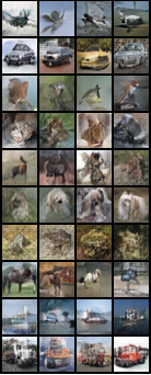
(a) COLA

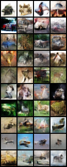
(b) GLO

Figure 1: Training on CIFAR-10 with no labels: the images generated by our method (left), which imposes semantic structure on the latent space, are superior to the alternative method (right). Each row holds a random sample from a distinct object class.

Generative image modeling is a long-standing challenge in computer vision. Unconditional generative models aim at learning the underlying distribution of the data using a finite training set, and synthesizing new samples from the learned distribution. Recently, deep generative models have shown remarkable results in synthesizing high-fidelity and diverse images. Most notably, Generative Adversarial Networks (GANs) [21] have been extensively used in classic computer vision tasks such as image generation, image restoration and domain translation, alongside traditional learning tasks such as data augmentation [18] and clustering [6, 46].

Since their inception, the unsupervised training of GANs achieved effective models able to produce natural-looking images, while relying on a simple and easily modified framework. Nevertheless, and despite numerous efforts for improvement, GANs still exhibit some critical drawbacks that arise from the adversarial nature of the optimization. These include: (i) an unstable training procedure, that is highly sensitive to the choice of initialization, architecture and hyper-parameters; (ii) often the learned distribution suffers from mode-collapse, in which only a subset of the real distribution is covered by the model, or mode-mixture, where different modes are mixed with each other. These problems are amplified when training data is scarce [62].

These drawbacks have motivated research into non-adversarial alternatives such as Variational Auto Encoders (VAE) [32] and Generative Latent Optimization (GLO) [8]. VAEs learn generative deep models that include a representation layer defining the model’s latent space, where both the prior and posterior distributions over the latent space are approximated by parametric Gaussian distributions. GLO learns a non parametric prior over the latent space in unison with the generative model. Although the VAE framework stands on solid theoretical foundations, VAEs generally do not generate sharp images, partially due to the restrictive parametric assumptions that are enforced. GLO, on the other hand, imposes hardly any limitation on the learned distribution over the latent space, which is guided only by the reconstruction performance of the model. Alas, as a result the structure of the latent space holds no semantic information, and cannot be effectively sampled from. These limitations are aggravated when dealing with multi-modal distributed data, as is typically the case with multi-class data.

Broadly speaking, most contemporary generative models rely on common and often implicit assumptions: (i) the Manifold Hypothesis, which assumes that real-world high-dimensional data lie on low-dimensional manifolds embedded within the high-dimensional space; (ii) that there exists a mapping from a low dimension latent space onto the real data manifold; (iii) that this latent space can be approximated by a single Gaussian distribution (such is the latent prior distribution in most variants of GANs, VAEs, and GLO); and (iv) that the generative model is capable of learning the assumed mapping. While these assumptions may hold true when trying to learn from data that resides on a single manifold, it is impossible for a continuous mapping (CNN generator) to effectively map a connected latent space onto a disconnected data manifold of a multi-class distribution [29].

In this work, we seek to overcome both the inherent drawbacks of the GAN framework and the deficiency of the uni-modal Gaussian prior in modeling the latent space. Thus, in Section 3 we propose an unsupervised non-adversarial generative model, that optimizes the latent space by fitting a multi-modal data distribution. Unlike GLO, our latent space preserves semantical information about the data, while the multi-modal distribution allows for the efficient and direct sampling of new data. As will be shown in Section 5, the distribution over the latent space that is learnt by our model captures semantic properties of the data. As a result, our model is capable of generating better images in terms of image quality, diversity and discriminability. In Section 4 we provide some theoretical justification for our method.

Expanding to domains where GANs do not excel, our model is designed to be applicable for downstream tasks where training data is scarce. The task of learning from small sample is usually tackled with the aid of external data or prior knowledge. While transfer-based techniques work well when the source and target domains share distributional similarities, it is not at all the case when the target data comes from a considerably different domain (such as medical imaging) [50, 42]. Furthermore, gaining access to large labeled datasets may not always be possible due to legal and ethical considerations. In contrast, here we tackle the small-sample classification task where no prior knowledge or external data is present. In this setting, the training algorithm may get as few as 5 images per class, having access to no additional labeled or unlabeled data. This constitutes a very challenging task. In Section 6 we show that, when using our model to augment the real data, we are able to advance the state-of-the-art and achieve top performance in small sample classification tasks.

Our main contributions are as follows:

• Introduce a novel unsupervised non-adversarial generative model capable of synthesizing diverse discriminable images from multi-class distributions (Section 3).

• Provide sufficient conditions and a simplified theoretical framework, under which our method can be beneficial in approximating under-sampled distributions (Section 4).

• Demonstrate superior image synthesis capabilities when training data is scarce, as compared to state-of-the-art GAN models (Section 5).

• Apply our model to small-sample classification tasks, surpassing all previous work in this domain (Section 6).

2 Recent Related Work

Modeling disconnected data manifolds.

The issue with mapping a connected latent space onto a disconnected data manifold was mainly addressed in the context of overcoming mode-collapse in GANs. [11, 37, 16, 57] use an encoder to match the latent code with the data distribution. While the latent representation of these methods is optimized via a reconstruction loss of the decoder, our method learns a representation that holds semantical information.

Another line of work [30, 3, 25, 19] uses multiple generators in order to cover all the modes in the data, while [1, 26] learn a mapping from a normally distributed noise to an optimized latent structure in a non-adversarial framework. Other works use a GMM prior over the latent space in VAEs [14, 55] and GANs [6]. Finally, [12] combines discrete and continuous latent factors to learn a disentangled representation of the data.

Data Embedding and Feature Learning.

Learning a meaningful low-dimensional embedding for high-dimensional data has been significantly improved by advances in deep neural networks and self-supervised learning. Thus, [10, 22, 27] all harness the large capacity of deep neural networks to learn efficient clustered representations of natural images. In a related line of work, self-supervised learning involves the learning of meaningful visual features from a pretext task using labels that are produced from the data itself with no direct supervision. These include jigsaw puzzle solving [48], predicting positions of patches in an image [15], and predicting image rotations (’RotNet’) [20]. In this work, we learn a clustered embedding of the data and a self-supervised pretext task en masse, which greatly improves the quality of the learned representation.

Learning from small sample.

Classification from small sample, with no prior knowledge or access to external data, has been chiefly approached by attempting to augment the sample into a sufficiently large training set. Thus DADA [65] adapts a GAN model for this purpose, TANDA [51] uses GANs to learn generic data augmentations composed of pre-defined transformations using large unlabeled data, DHN [49] uses a hybrid network that incorporates learnable weights with a scattering network of predefined wavelets, and CFVAE-DHN [40] augments the latent variables of a VAE, which in turn generates additional data that is classified using a DHN. Likewise, [5] promotes the use of the cosine-loss, and [9] promotes low-complexity networks.

Other methods usually incorporate some form of transfer learning [66], where parameters that are learned in a source domain are transferred and utilized in a different target domain. Transfer learning from large datasets to smaller ones has also been investigated in generative models [61, 58, 47, 59]. One recent prominent research paradigm in this context is termed few-shot learning [60]. We consider this paradigm to be an instance of transfer (or meta) learning and not strict classification from small sample, as it requires access to an external labeled dataset.

3 Proposed Method

3.1 COLA: Unsupervised Algorithm

Our method, Clustered Optimization of LAtent space (COLA), is an unsupervised method which learns a generative model for the synthesis of images. The method is designed to cope with a small training set of natural images, portraying distinct object categories. It involves three steps, the first two of which are illustrated in Fig. 2. Our code is supplied in the supplementary materials.

Step I: Clustering the latent space.

The goal here is to deliver a mapping from the data space to a latent space, while clustering the mapped points into compact $K$ clusters, see illustration in Fig. 2. To this end we train a deep convolutional network $E_{\theta}$, which maps each data point to a fixed low-dimensional target point in the latent space - the unit sphere in $\mathbb{R}^{K}$. The target is sampled from a pre-defined distribution over the latent space.

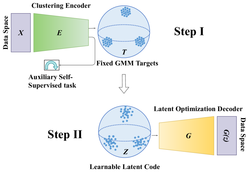
Figure 2: Illustration of our model: In step I images are mapped to fixed low-dimensional targets $T$. In step II these targets form a latent space $Z$ that is trained in conjunction with the generator parameters to reconstruct the original image.

Specifically, given an unlabeled dataset $\mathcal{X}=\{x_{i}\}_{i=1}^{N}$, the model is initialized with some random assignment $\{(x_{i},\bm{t}_{i})\}_{i=1}^{N}$, where each $\bm{t}_{i}\in\mathbb{R}^{K}$ is sampled from a GMM distribution with K-components, and normalized to length 1. Training involves the minimization of

$$\|E_{\theta}(x_{i})-\bm{t}_{\pi(i)}\|_{2}^{2}$$ (2)

over the assignment $\{(x_{i},\bm{t}_{\pi(i)})\}_{i=1}^{N}$ and parameters $\theta$.

This optimization problem is solved with SGD, and involves two steps per mini-batch. First, the sample $\{x_{i}\}_{i\in b}$ is mapped onto the latent space. The assignment problem for $\{(x_{i},\bm{t}_{\pi(i)})\ |i\in b\}$ is solved using the Hungarian Algorithm [36] applied to the following problem:

$$\pi^{*}=\operatorname*{arg\,min}_{\pi:b\leftrightarrow b}\sum_{i\in b}\|E_{\theta}(x_{i})-\bm{t}_{\pi(i)}\|_{2}^{2}$$ (3)

Subsequently $\pi^{*}$ is inserted into Eq. 2, which is then optimized w.r.t $~{}\theta$. A full formulation and implementation details can be found in Alg. 2 and Section B.1 respectively in the Appendix. Alg. 2 is enhanced with self-supervision based on the auxiliary ’RotNet’ task [20], and consistency regularization where augmented images are mapped to the same cluster.

The output of this model constitutes a latent space, where the representations of semantically similar images reside in proximity, and images from distinct classes are located further apart. This representation is used to initialize the latent space of the generative model in step II. To simplify the presentation, henceforth we let $\bm{t}_{i}=\bm{t}_{\pi^{*}(i)}$ denote the final target associated with $x_{i}$.

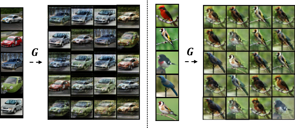
Figure 3: Synthetic images generated by our model when trained on STL-10 with 5 images per class and no external data. Real images are shown on the left, synthetic images are shown on the right.

Step II: Image generation.

Given a matching between data points $\mathcal{X}$ and targets $\mathcal{T}$ - $\{(x_{i},\bm{t}_{i})\}_{i=1}^{N}$, a latent code $\mathcal{Z}=\{\bm{z}_{i}\}_{i=1}^{N}$ is constructed such that

$$\bm{z}_{i}=(\frac{\bm{t}_{i}}{\|\bm{t}_{i}\|_{2}},\frac{\bm{v}_{i}}{\|\bm{v}_{i}\|_{2}})\in\mathbb{R}^{K+d}$$

Above $\bm{v}_{i}\sim\mathcal{N}(\vec{0},\sigma I_{d\times d})$ denotes an additional source of variation, and $\bm{t}_{i}$ denotes the class-component of the code.

The parameters of a CNN generator function $G_{\theta}:\mathcal{Z}\longrightarrow\mathcal{X}$ are optimized in conjunction with the learnable representation vectors $\mathcal{Z}$, as illustrated in Fig. 2. The optimization problem is defined as: min_θ,Z 1N ∑_i=1^N L_rec(G_θ(z_i), x_i)  s.t.  ∥z_i∥_2 = 1 where $\mathcal{L}_{rec}$ denotes the reconstruction loss between the original image $x_{i}$ and the image generated by the model $G_{\theta}(z_{i})$.

As shown in [26], the best image quality for this kind of models may be obtained when $\mathcal{L}_{rec}$ is realized with the perceptual loss [28]: L_vgg(x,x’) = —x - x’—  + ∑_layers:  i^k —l_i(x) - l_i(x’)—

In (3.1) $l_{i}$ denotes the perceptual layer in a pre-trained VGG network [56]. Nevertheless, since external data cannot be used in the small sample scenario adopted here, $\mathcal{L}_{rec}$ is realized in our method with the Laplacian Pyramid loss: L_lap(x,x’) = —x - x’—  +γ∑_i^k 2^-2i —L_i(x) - L_i(x’)—

In (3.1) $L_{i}(x)$ denotes the i-th level of the Laplacian pyramid representation of $x$ [41]. The sum of differences is weighted to preserve the high-frequencies of the original image. The components of the representation vectors are normalized after each epoch to length 1, projecting them back to the unit spheres in $\mathbb{R}^{K},\mathbb{R}^{d}$ respectively.

This step is summarized below in Alg. 1. Full implementation details are presented in Appendix B.2.

Step III: posterior distribution over the latent space.

After training, a posterior distribution over the latent space is obtained by fitting a unique multivariate Gaussian to each cluster in the latent space. Sampling is then performed from the uniform mixture of these Gaussian distributions.

Algorithm 1 : Training the Generative Model

INPUT:

matched pairs $\{(x_{i},\bm{t}_{i})\}_{i=1}^{N}\subset X\times[0,1]^{K}$ from step I

$G_{\theta}$ - CNN Generator with parameters $\theta$

$\lambda^{\theta}_{e},\lambda^{z}_{e}$ - learning rate at epoch e of $\theta,Z$

$\sigma$ - pre-defined latent std

for i=1…N do $\triangleright$ initialize latent space

     sample $\bm{v}_{i}\sim\mathcal{N}(\vec{0},\sigma I_{d\times d})$

     $\bm{z}_{i}\leftarrow(\frac{\bm{t}_{i}}{\|\bm{t}_{i}\|_{2}},\frac{\bm{v}_{i}}{\|\bm{v}_{i}\|_{2}})\in\mathbb{R}^{K+d}$

end for

for e=1…epochs do

     for i=1…iters do

         sample batch $\{(x_{i},\bm{z}_{i})|i\in B\}$

$$\mathcal{L}_{B}=\frac{1}{|B|}\sum_{i\in B}\mathcal{L}_{rec}(x_{i},G_{\theta}(\bm{z}_{i}))$$

         $\theta\leftarrow\theta-\lambda^{\theta}_{e}(\nabla_{\theta}\mathcal{L}_{B})$

         $\bm{z}\leftarrow\bm{z}-\lambda^{z}_{e}(\nabla_{z}\mathcal{L}_{B})$

     end for

       $\bm{t}\leftarrow\bm{z}_{[1:K]},\quad\quad\bm{v}\leftarrow\bm{z}_{[K+1:K+d]}$

     $\forall_{i}\quad\bm{z}_{i}\leftarrow(\frac{\bm{t}_{i}}{\|\bm{t}_{i}\|_{2}},\frac{\bm{v}_{i}}{\|\bm{v}_{i}\|_{2}})$$\triangleright$ Normalize inputs

end for

3.2 sCOLA: Supervised Algorithm

In the supervised framework, we have a labeled dataset with $K$ classes $\mathcal{X}=\{(x_{1},y_{1}),(x_{2},y_{2}),\cdots,(x_{N},y_{N})\}$, where $y_{i}\in[K]$ denotes the class label of $x_{i}$, and $\bm{e}_{y}^{i}$ denotes the one-hot representation of the labels. The supervised version of our method, sCOLA includes steps II and III of COLA. The clustering in step I is replaced by the supervision labels from the training data, where each $\bm{t}_{i}$ is replaced by the corresponding $\bm{e}_{y}^{i}$. Fig. 3 shows images generated by our model with only 5 training examples per class.

4 Theoretical Analysis

Stripped off its technical details, the method in Section 3 essentially learns a noisy surrogate distribution $Z$ to approximate the real data distribution $X$ and generate new data. In this paper, our ultimate goal is not to generate new high quality data, but rather to estimate some function $f:X\longrightarrow\Omega$ from a sample of $X$. When $X$ denotes data sampled from $K$ discrete classes, a multi-class classifier is such a function whose codomain is either $[K]$ or $\mathbb{R}^{K}$. If the sample of $X$ is too small, the surrogate distribution $Z$ can be used to generate more data and improve the estimation of $f$. The analysis below identifies sufficient conditions on the respective sample sizes, such that improvement can indeed be guaranteed.

Notations.

Assume an i.i.d. sample of random variable pairs - $\{X_{i},Y_{i}\}_{i=1}^{N}$, where $X_{i}/_{Y_{i}=k}\overset{iid}{\sim}\mathcal{D}_{k}$ and $\mathcal{D}_{k}$ denotes the class conditional distributions of variable $X$. Let $\mathcal{X}_{k}$ denote the conditional sub-sample of datapoints from class $k$: $\mathcal{X}_{k}=\{X_{i_{j}},Y_{i_{j}}/_{Y_{i_{j}}=k}\}_{j=1}^{m_{k}}$, where $\sum_{k=1}^{K}m_{k}=N$.

For simplicity, we will assume in our analysis that $f$ depends only on the expected value of the conditional distributions $\{\mathcal{D}_{k}\}_{k=1}^{K}$, denoted $\mu_{k}$. Let $\tilde{\mu}_{k}(X)$ denote an estimator of $\mu_{k}$ from an iid sample of random variable $X$. Our task is to obtain a set of good estimators $\{\tilde{\mu}_{k}\}_{k=1}^{K}$. In order to simplify the notations, we shall henceforth drop the class index k, with the understanding that the following analysis does not depend on $k$.

In accordance, let $\mathcal{X}^{m}$ denote an iid sample of size $m$ from the real conditional distribution $X$ of some class $k$, and $\mathcal{Z}^{n}$ denote an iid sample of size $n$ from the class surrogate distribution $Z$. Let $\mu_{x}=\mu$ denote the expected value of $X$, and $\mu_{z}$ denote the expected value of $Z$, where $|\mu_{x}-\mu_{z}|=d$. Let $\bar{\mathcal{X}}^{m}$ and $\bar{\mathcal{Z}}^{n}$ denote the population means of the two samples respectively. Recall that $Var[\bar{\mathcal{X}}^{m}]=\frac{Var[X]}{m}$ and $Var[\bar{\mathcal{Z}}^{n}]=\frac{Var[Z]}{n}$.

As customary, we use the population mean of each sample to estimate the unknown distribution’s mean $\mu$. Accordingly:

$$\begin{split}\tilde{\mu}(X)&=\bar{\mathcal{X}}^{m}\\ \tilde{\mu}(Z)&=\bar{\mathcal{Z}}^{n}\end{split}$$ (4)

The error of the two estimators is measured as follows:

$$\begin{split}Err(X)&=(\bar{\mathcal{X}}^{m}-\mu)^{2}\\ Err(Z)&=(\bar{\mathcal{Z}}^{n}-\mu)^{2}\end{split}$$ (5)

Proposition 1.

If $Var[X]>md^{2}$, then

$$n\geq\frac{mVar[Z]}{Var[X]-md^{2}}~{}\implies~{}\mathbb{E}[Err(Z)]\leq\mathbb{E}[Err(X)]$$

Proof.

$$\begin{split}\mathbb{E}[Err(Z)]&=\mathbb{E}[(\bar{\mathcal{Z}}^{n}-\mu)^{2}]~{}~{}~{}~{}~{}~{}~{}~{}~{}~{}~{}~{}~{}~{}~{}~{}{\color[rgb]{0.36,0.54,0.66}(\textrm{use}~{}\mu=\mu_{x})}\\ &\leq\mathbb{E}[(\bar{\mathcal{Z}}^{n}-\mu_{z})^{2}]+d^{2}=\frac{Var[Z]}{n}+d^{2}\end{split}$$

As long as $Var[X]>md^{2}$

$$n\geq\frac{mVar[Z]}{Var[X]-md^{2}}~{}\implies~{}\frac{Var[Z]}{n}+d^{2}\leq\frac{Var[X]}{m}$$

and therefore

$$\mathbb{E}[Err(Z)]\leq Var[\bar{\mathcal{X}}^{m}]=\mathbb{E}[Err(X)]\qed$$

Corollary 1.1.

For each class $k$, if the sample of the surrogate random variable $Z$ is sufficiently large

$$n\geq\frac{mVar[Z]}{Var[X]-md^{2}}$$

then the estimator of classifier $f$ obtained from $\mathcal{Z}^{n}$ is more accurate than the estimator obtained from $\mathcal{X}^{m}$.

Proposition 2.

Assume that $Pr[0\leq X,Z\leq 1]=1$, which can be achieved by dataset normalizing. Then $\forall\epsilon>d$, if $n\geq m(\frac{\epsilon}{\epsilon-d})^{2}$, then the bound obtained by the Hoeffding’s inequality on $Pr(|Err(Z)|\geq\epsilon)$ is tighter than the corresponding bound on $Pr(|Err(X)|\geq\epsilon)$.

Proof.

We invoke the Hoeffding’s inequality:

$$Pr(|\bar{\mathcal{X}}^{m}-\mu|>\epsilon)\leq 2e^{-2m\epsilon^{2}}$$

and note that

$$|Err(Z)|\leq|\bar{\mathcal{Z}}^{n}-\mu_{z}|+|\mu_{x}-\mu_{z}|=|\bar{\mathcal{Z}}^{n}-\mu_{z}|+d$$

It follows that

$$\begin{split}Pr(|Err(Z)|\geq\epsilon)&\leq Pr(|\bar{\mathcal{Z}}^{n}-\mu_{z}|+d\geq\epsilon)\\ &=Pr(|\bar{\mathcal{Z}}^{n}-\mu_{z}|\geq\epsilon-d)\\ &\leq 2e^{-2n(\epsilon-d)^{2}}:=B(Z)\\ Pr(|Err(X)|\geq\epsilon)&=Pr(|\bar{\mathcal{X}}^{m}-\mu_{x}|\geq\epsilon)\\ &\leq 2e^{-2m\epsilon^{2}}:=B(X)\end{split}$$

Finally

$$n\geq m(\frac{\epsilon}{\epsilon-d})^{2}\implies B(Z)\leq B(X)\qed$$

Corollary 2.1.

For each class $k$, if the sample from the surrogate random variable $Z$ is sufficiently large

$$n\geq m(\frac{\epsilon}{\epsilon-d})^{2},$$

then the estimator of classifier $f$ obtained from $\mathcal{Z}^{n}$ is more confident than the estimator obtained from $\mathcal{X}^{m}$.

5 Image generation, Large and Small Sample

We shall now demonstrate the capability of our model to produce diverse and discriminable images, employing evaluation metrics that quantify these attributes. Firstly, we compare our model with competitive conditional GAN models that use large and computationally heavy architectures. While these models maintain superiority on large datasets, this dominance diminishes as the sample size drops. Secondly, we show that our unsupervised variant surpasses other unsupervised generative adversarial models using the same architecture. Lastly, we show that our model consistently outperforms other non-adversarial methods in terms of image quality and diversity, regardless of sample size.

5.1 Methodology

Datasets

The datasets we use are included in Table 1.

Evaluation scores.

Designing meaningful quantitative evaluation measures for generative models is a challenging ongoing research area. Presently two scores seem to dominate the field: the Inception Score [53], and the Fréchet Inception Distance (FID) [24]. Noting that the Inception score does not take into account the real data distribution and cannot capture intra-class diversity, we will not be using this metric in our evaluation.

FID compares the statistics of activations in the penultimate layer of the Inception network (trained on ’ImageNet’) between real and generated images, computing the distance between the uni-modal Gaussian distributions that best fit the activation patterns. This score has two major drawbacks: (i) it captures image quality and diversity on a single scale, and therefore cannot distinguish between the two factors; (ii) it is based on the Inception network that has been trained with 1,000 classes of ’ImageNet’, and may not be suitable for all datasets [4]. In Appendix A we show that the FID score also fails to reveal intra-class diversity, making it less useful for multi-class datasets (see also [43]). Implementation details for the FID score used in our experiments can be found in Appendix B.4.

Given the problems discussed above, we seek an additional score that can reliably measure how well the generated images fit the true distribution of the data. More importantly, considering that generative models are commonly used in down-stream tasks, we seek a score that can measure the usefulness of the model generations in such tasks. To this end we adopt the scores proposed in [54] (’GAN-Train’) and [52] (’CAS’), which are based on training a classification network on the generated images, and evaluating it on real images. The classification accuracy of this network forms an implicit measure of the recall and precision of the generated dataset, since it can only achieve a high score if the synthetic data is sufficiently diverse and discriminable. In our experiments, we follow the protocol defined in [52].

Generative methods used for comparisons.

We compare our model against state-of-the-art generative models, one adversarial model based on the GAN framework, and a second non-adversarial method:

1. Adversarial CGAN-PD [45]: a conditional GAN with Projection-Discriminator, trained and implemented in accordance with [39].

2. Non-adversarial GLO [8]: the original model augmented with the superior perceptual loss from Eq. 3.1. Similarly to step III above, after training we fit a Gaussian Mixture Model to the learned latent space.

Implementation details can be found in Appendix B.2.

5.2 Results

Unsupervised.

In the unsupervised scenario, we compare our model to the baseline GLO model, see Fig. 5. Clearly our model outperforms GLO on all datasets and metrics, and produces significantly better looking images as demonstrated in Fig. 1. Furthermore, we recall that different GAN models can reach similar FID scores if given a high enough computational budget [44]. We therefore adopt the fair comparison protocol proposed in [44], where the architectures of all the models are fixed to the one used in ’InfoGAN’ [12], and all models possess the same computational budget for hyper-parameter search. In this protocol, our method outperforms all GAN variants and is on par with the state-of-the-art non-adversarial methods, see Fig. 4.

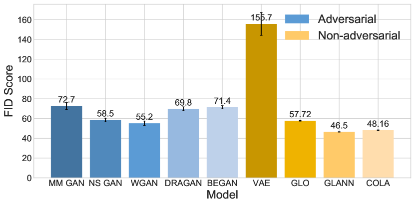
Figure 4: FID score computed for CIFAR-10, when all models share the same architecture of ’InfoGAN’ [12]. Unlike all other models in this comparison, our method allows for the sampling of images from different individual classes.

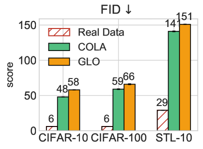
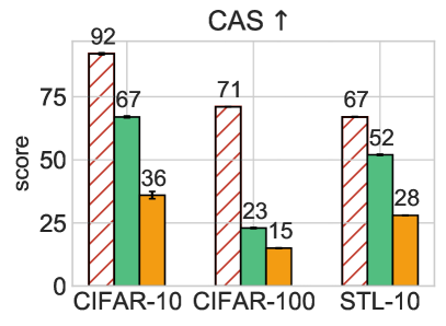
Figure 5: Comparison between GLO and COLA using the FID and CAS scores. Our model shows a clear advantage in all cases.

Supervised.

When learning from fully labeled datasets, we evaluate our model against the state-of-the-art conditional GAN variant CGAN-PD with varying sample sizes. Results are shown in Fig. 7.

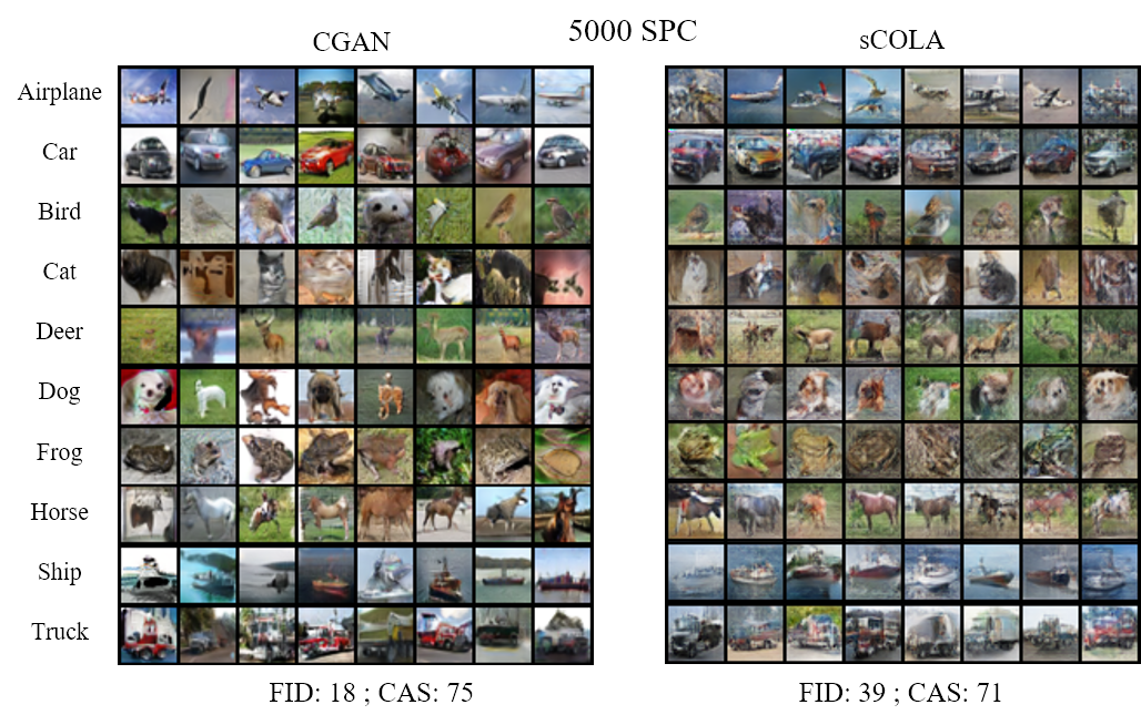
Figure 13: visualization of generations of CGAN (left) and sCOLA (right) trained on CIFAR-10 with varying samples per class (spc). While CGAN suffers from mode-collapse when training data drops, our method maintains a an intra-calss diversity that better matches the original data.

Although conditional GANs obtain better FID scores on large datasets, their performance deteriorates rapidly when training size decreases. Furthermore, our model outperforms GANs when consulting the CAS score on almost all configurations. A qualitative comparison presented in Fig. 8 and in Fig. 13 in the Appendix suggests that this deterioration may be attributed to the mode-collapse manifested in CGAN when trained with insufficient data. In contrast, in the extreme small sample regime the images synthesized by our model can hardly be distinguished from real images by both scores, suggesting superior generalization ability in this regime.

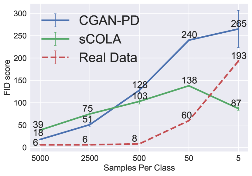
(a) FID $\downarrow$

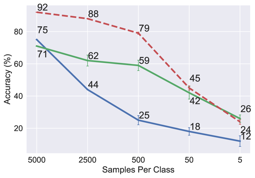
(b) CAS $\uparrow$

(c) CIFAR-10

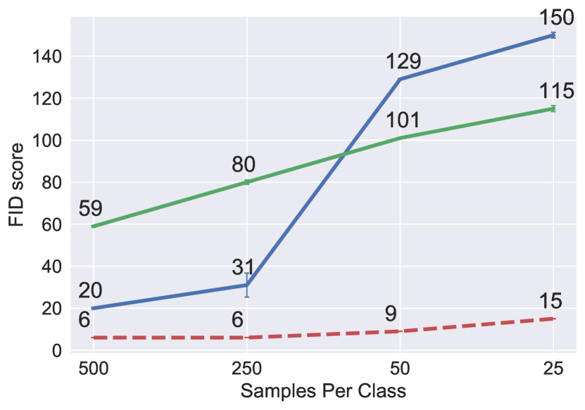
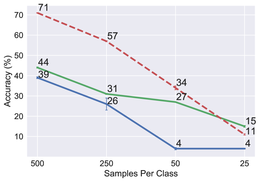
(d) CIFAR-100

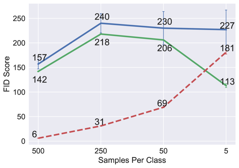
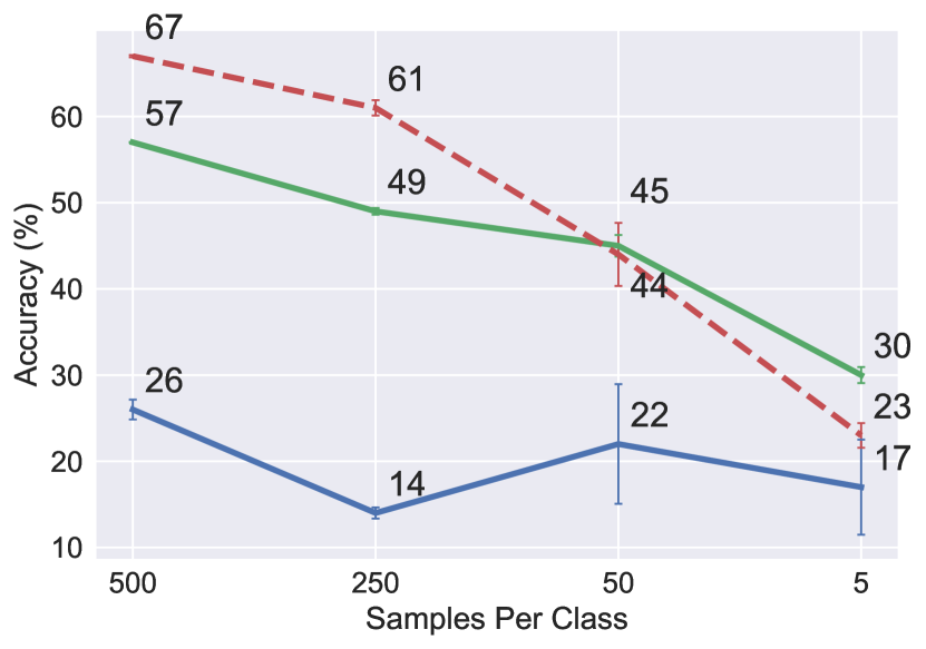
(e) STL-10

Figure 7: FID (left) and CAS (right) scores on CIFAR-10, CIFAR-100 and STL-10 with varying training sample sizes. sCOLA’s generated images achieve better scores than the GAN’s images in the small sample regime, and even achieve better scores than real images when data is extremely scarce (see also Section 6).

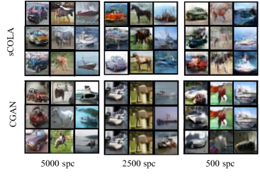
Figure 8: qualitative comparison between sCOLA (top) and CGAN (bottom) trained on CIFAR-10 with varying numbers of samples per class (spc). Each column corresponds to a different class in the data. CGAN evidently suffers from mode-collapse when given insufficient data for training.

6 Classification from Small Sample

In this section we show the benefits of using our method in the small sample regime, where only a small sample is available to train the classifier, and no external information can be used. We will show that using our model to augment the small training set significantly improves the performance of a deep network classifier trained on this data.

Classification approach.

sCOLA is first trained on the small training sample, and then used to generate novel samples from each class. The synthetic images are then combined with the real images, resulting in an extended training set (termed ”Mix”) that consists of 50% real images, and 50% synthetic images generated by our model. This extended set is then used to train a CNN classifier. For comparison, we train the same CNN classifier with the original images, making sure that both methods see the same subset of images with an identical training procedure.

6.1 Methodology

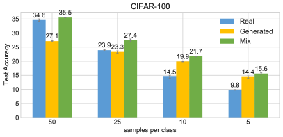
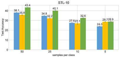
Figure 9: Classification accuracy for CIFAR-100 (left) and STL-10 (right) with varying sample size per class.

Name	Classes	SPC Train/Test	Dimension
CIFAR-10 [35]	10	5000 / 1000	$32\times 32\times 3$
CIFAR-100 [35]	100	500 / 100	$32\times 32\times 3$
STL-10 (downsampled, labeled only) [13]	10	500 / 800	$48\times 48\times 3$
Tiny ImageNet [38]	200	500 / 50	$64\times 64\times 3$

Table 1: Datasets used in our experiments.

The datasets we use are described in Table 1. For each dataset we train our method with various sample sizes, ranging from 100 samples per class (spc) to as low as 5 spc. For each sample size we run our model on 3 random samples of the same size, and evaluate the classifier’s accuracy on the original held-out test set of the data. In order to isolate the contribution of our approach from other factors, we fix the classifier’s architecture to an off-the-shelf ResNet-20 [23] for all datasets except for Tiny ImageNet, which, due to its larger size, resolution and number of classes, necessitates the use of a larger network. Consequently we use the same WRN-16-8 [63] network as CFVAE-DHN (excluding DHN initialization). Full implementation details can be found in Appendix B.3.

6.2 Empirical Results

We compare our model trained on CIFAR-10 and Tiny ImageNet with the best published results reported in [40]. A short description of these methods can be found in Section 2. The results are summarized in Table 2. Our method achieves the best results across all sample sizes on both datasets.

CIFAR-10
100 50 20 10 5 DADA 48.32 $\pm{.23}$ 40.48 $\pm{.57}$ 30.44 $\pm{.37}$ 21.67 $\pm{.58}$ - Tanda 45.17 $\pm{1.84}$ 39.16 $\pm{1.18}$ 29.84 $\pm{1.23}$ 20.18 $\pm{.73}$ - CFVAE-DHN 55.58 $\pm{.12}$ 52.06 $\pm{.36}$ 32.65 $\pm{.38}$ 34.11 $\pm{.67}$ - sCOLA 58.59 $\pm{0.58}$ 54.51 $\pm{0.22}$ 49.63 $\pm{1.29}$ 42.86 $\pm{2.04}$ 29.05 $\pm{1.09}$

Tiny-ImageNet
100 50 20 10 DADA 17.64 $\pm{.82}$ 14.97 $\pm{1.08}$ 10.13 $\pm{2.04}$ - Tanda 27.07 $\pm{.94}$ 17.95 $\pm{.59}$ 13.92 $\pm{.59}$ - CFVAE-DHN 35.97 $\pm{.35}$ 28.82 $\pm{.79}$ 21.37 $\pm{.29}$ - sCOLA 35.24 $\pm{.34}$ 29.70 $\pm{.05}$ 23.99 $\pm{.52}$ 17.14 $\pm{.27}$

Table 2: Classification accuracy for CIFAR-10 (top) and Tiny-ImageNet (bottom). Each column corresponds to a different sample size per class. The architecture used by our method is smaller or similar to the ones used by the other methods (see methodology).

Additionally, we expand our experiments to datasets with no published results to date on small sample classification tasks. For these datasets, we show that when a classifier is trained on a mixed dataset consisting of real and synthetic images, it yields better results compared to those obtained when being trained only on the real images or only on the synthetic images. This suggests that our model succeeds in learning the data distribution well enough, and can subsequently generate novel samples that do not exist in the real data. Fig. 9 shows results on CIFAR-100 and STL-10.

6.3 Ablation Study

An ablation study probing different components of our method, including image similarity measure, architecture of the generator and classification network, can be found in Section C in Supp. In this regard, we found that the size of the classifier has little effect on the overall performance when dealing with very small samples.

7 Summary and Discussion

We described a novel unsupervised non-adversarial generative model that is capable of generating diverse multi-class images. This model outperforms previous non-adversarial generative methods, and outperforms more complicated GAN models when the training sample is small.

Unlike GAN models, our model is characterized by stable and relatively fast training, it is relatively insensitive to the choice of hyper-parameters, and it has control over each class variance in the synthesized dataset. Furthermore, empirical results show that our method is robust to the risk of mode-collapse, which plagues most GAN models when trained with insufficient data.

We further demonstrated the capability of our model to augment small data for classification, advancing the state-of-the-art in this domain. Since our method is only used to augment the small sample, it remains orthogonal to future advances in algorithms devised for small training sets.

Appendix

A The FID score is inadequate for multi-class datasets

In this section we will show that the FID fails to reveal intra-class variance, highlighting its inadequacy to serve as a single metric for assessing generative models on multi-class data. To do so, we will use our model to construct two datasets that obtain similar FID scores, but exhibits an apparent difference in terms of the intra-class variance. We notice that generating images from latent codes that reside in proximity yields images that are visually and semantically similar. On the other hand, sampling latent codes that come from the same latent cluster but with a greater distance from each other, yields far more diverse outputs under the model. An example of this effect is illustrated in Fig. 10

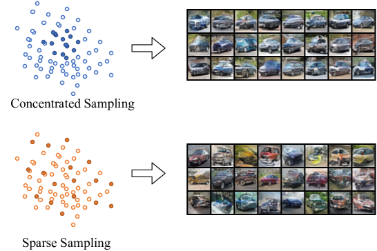
Figure 10: The effect of the scattering of latent codes on the generated images. in the top row, latent codes that are sampled around the cluster means result in similar images with small intra-class variation. In the bottom row, latent codes that are sparsely sampled result in images that exhibit a greater intra-class variance.

Consequently, we can generate two versions of synthesized datasets- one where each class is generated from concentrated latent codes, and one where each class is generated from sparsely sampled latent code from the same cluster. The first dataset will consist of homogeneous classes, exhibiting a small intra-class variance whereas the second one will hold classes with a larger variety of objects.

In this experimental setting, we use our model to generate two synthetic versions of CIFAR-10- one which we will term ’concentrated’ which is made of generations sampled from latent codes concentrated around the cluster means, and a second dataset, termed ’sparse’ which is based on sparsely sampled latent codes from the same cluster. We then evaluate these synthetic datasets using the FID and CAS scores.results are presnted in Fig. 11

Since the ’concentrated’ dataset has low intra-class variation, each class consists of similar images, which makes it an inferior dataset for training a classifier (as is evident by the low accuracy obtained by a classifier trained on this data). On the other hand, the ’sparse’ dataset is characterised by a higher intra-class variance, with diverse images in each class, yielding an effective training set for classification. Nevertheless, the FID scores of the two datasets are barely affected by these differences, since it is based on a single multivariate Gaussian approximation of their activations in the penultimate layer of the Inception network, which cannot capture intra-class variance.

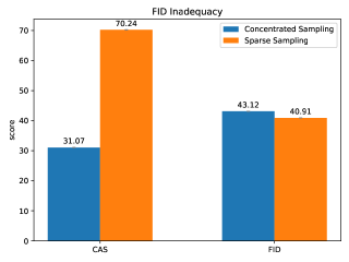
Figure 11: While the CAS score is an informative measure of the intra-class variance, the FID fails to discriminate between the two datasets.

Algorithm 2 Clustering the Latent Space

INPUT: Unlabeled dataset $\{x_{i}\}_{i=1}^{N}$

$K$ - number of clusters

$E_{\theta}$ - dual-head CNN Encoder with parameters $\theta$

$E_{\theta}^{1}(x)\in\mathbb{R}^{K};E_{\theta}^{2}(x)\in\mathbb{R}^{4}$

$\{\xi:X\rightarrow X\}$ random augmentation functions

$\sigma$ - intra-class variance

$\lambda_{e}$ - learning rate at epoch e

OUTPUT: a matching $\{(x_{i},t_{i})\}_{i=1}^{N}$ such that $\{t_{i}\}_{i=1}^{N}$ are clustered according to their matching $x_{i}$

for $i$=1 to $N$ do $\triangleright$ initialize a random matching

     sample $c\sim Categ(\frac{1}{K},...\frac{1}{K})$

     sample $v\sim\mathcal{N}(\vec{\mu_{c}},\sigma I_{K\times K})$

     $t_{i}\leftarrow\frac{v}{||v||_{2}}$ , $A\leftarrow\{(x_{i},t_{i})\}_{i=1}^{N}$

end for

for e=1…epochs do

     for i=1…iters do

         sample batch $(X^{b},Z^{b})$

         solve the assignment problem for $\{(x_{i},t_{i})\}_{i=1}^{b}$

         using the Hungarian Algorithm

         

$$\pi^{*}\leftarrow\operatorname*{arg\,min}_{\pi:[b]\leftrightarrow[b]}\sum_{j}||E_{\theta}^{1}(x_{j})-t_{\pi(j)}||_{2}^{2}$$

         

$$\theta\leftarrow\theta-\lambda_{e}\nabla_{\theta}\sum_{j}\sum_{\xi}||E_{\theta}^{1}(\xi(x_{j}))-t_{\pi^{*}(j)}||_{2}^{2}$$

         $\forall i\in b\quad A(x_{i})=t_{\pi^{*}(i)}$ $\triangleright$ update assignments

     end for

     for i=1…iters do

         sample batch $(X^{b})$ $\triangleright$ rotate batch

         $X_{R}^{b}\leftarrow\big{\{}(X^{b})_{r}|r\in\{0^{\circ},90^{\circ},180^{\circ},270^{\circ}\}\big{\}}$

$$\theta\leftarrow\theta-\lambda_{e}\nabla_{\theta}\frac{1}{|X^{b}_{R}|}\sum_{i\in b}l_{ce}(E_{\theta}^{2}(x_{i}),r(x_{i}))$$

$\triangleright$ $l_{ce}$ is the cross-entropy loss

     end for

end for

B Implementation details

B.1 Step I - Clustering the latent space.

For all experiments we use a ResNet-18 [23] network for the encoder. The network is trained with SGD with an initial learning rate of 0.05 and momentum of 0.9 for 200 epochs. Learning rate is decayd by a factor of 0.5 every 50 epochs. Training is done sequentially where an epoch optimizing the target assignment problem is followed by an epoch optimizing the rotation prediction problem. In both cases we use a batch size of 128, where in the target assignment problem images are augmented by cropping, flipping and color jitters, and in the rotation prediction task each image is rotated in all orientations, yielding a batch size of 512. Weight decay regularization of 0.0005 is used on all datasets.

B.2 Step II - Image generation.

In all our experiments we used the ADAM optimizer [31], with an initial learning rate of 0.01 for the latent code, and 0.001 for $G_{\theta}$. The generative model was trained for 500 epochs, learning rate was decayed by 0.5 every 50 epochs. The only parameters that change throughout our experiments are the choice of architecture for the generator, the choice of reconstruction loss and the dimensionality of the latent space as follows:

1. Small-Sample: In this section, the generative function $G_{\theta}$ shares the same CNN generator architecture used in InfoGAN [12] (which is also the architecture used in GLO [8]). The dimension of the latent space was set to $\mathcal{Z}\subset\mathbb{R}^{K+d}$ where K is the number of classes in the dataset, and $d=64$ for all datasets. $\mathcal{L}_{rec}$ is implemented using the unsupervised Laplacian-Pyramid loss Eq. 3.1. An ablation study of different similarity measures is presneted in Section C.1.

2. Full Data: In the supervised version (sCOLA), the generative function $G_{\theta}$ shares the same CNN generator architecture used in CGAN [45], while in the unsupervised framework (COLA) we use the generator of InfoGAN [12]. In both versions $d=128$, and $\mathcal{L}_{rec}$ is implemented using the perceptual loss Eq. 3.1.

B.3 Small-sample classification

For a fair comparison, we use the same training procedure on all data sizes. i.e. same batch size, number of epochs, iterations per epoch and learning schedule.

ResNet-20 was trained for 180 epochs, with an initial learning rate of 0.1, decayed by 0.5 every 30 epochs. Whereas WRN-16-8 was trained for 200 epochs with an inital learning rate of 0.1, decayed by 0.2 every 60 epochs. Both networks were trained using SGD optimization with a batch size of 128. An ablation study showing the effect of different architectural designs, is presented in Section C.2. The classifier was trained using standard data augmentation with such image transformations as random flip and crop.

B.4 FID score implementation

For CIFAR-10 and CIFAR-100, FID scores were computed on a sample of 10K generated images against the default Test-set of size 10K. Each model was trained 3 times, and the final score was taken as the average over 10 random samples from each model.

For STL-10, FID scores were computed on a sample of 8K generated images against the default Test-set of size 8K. Note that most generative models that had been evaluated on this dataset used the whole dataset, including the 100K unlabeled images. Therefore these previous results are not comparable to the experimental results reported here.

C Ablation Study

C.1 Image similarity measure

Many generative models are trained using some form of reconstruction loss that is based on a similarity measure between the original image and the one reconstructed by the model. Since using the Euclidean distance in pixel space is highly inadequate (similar objects may differ drastically in pixel space) alternative similarity measures that capture the perceptual relationship between images have been thoroughly investigated in recent years. In this context, it has become a common practice to use a perceptual loss based on a VGG network that was pre-trained on ImageNet for image synthesis tasks [17, 28, 26]. Later works [64] have evaluated numerous similarity measures that are based on deep features of neural nets and concluded that they exhibit a strong correlation with human judgment even when these features where obtained in an unsupervised or self-supervised manner. Nevertheless, establishing a similarity measure without large amounts of data remains to this date an uncharted territory. In order to make our model applicable in the small-data regime, we seek a meaningful similarity measure that uses little to no data. Furthermore, while most works in this area have evaluated the similarity measure according to human judgment on image quality, we sought a measure that will also prove useful in downstream tasks. To this end, we have investigated various methods and evaluated them on the downstream task of image classification of the generated images. Results on partitions of size 1% of CIFAR-10 can be found in Fig. 12. We found that the Laplacian Pyramid Loss used in [8] yields the best results compared to other unsupervised measures. The loss functions that were compared are as follows:

1. ImageNet VGG16 - The original perceptual loss described in Eq. 3.1

2. Laplacian Pyramid - The Laplacian Pyramid Loss as described in Eq. 3.1

3. k-means ResNet32 - Perceptual distance based on layers of ResNet32 initialized with stacked k-means as described in [34]

4. Random ResNet32 - Perceptual distance based on layers of ResNet32 initialized with random weights

5. CIFAR-10 ResNet32 - Perceptual distance based on layers of ResNet32 trained on CIFAR-10

6. L1 - The $\mathcal{L}_{1}$ loss in pixel space

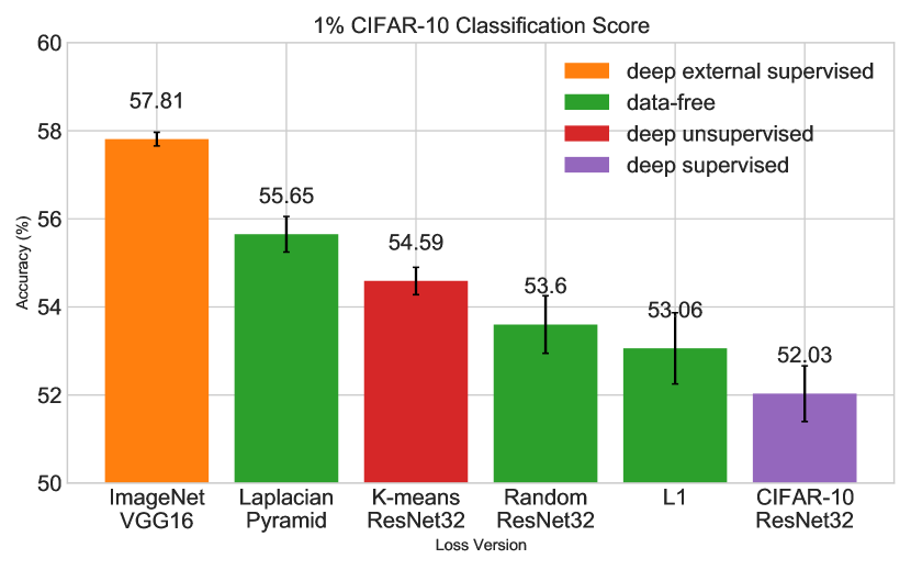
Figure 12: The effect of different similarity measures in the optimization of sCOLA when trained on on 1% of the images in CIFAR-10. Classification score is obtained using the same framework described in Section B.3

C.2 Small Data Classifier Architecture.

We experimented with various architectures to check whether larger networks are preferable over smaller ones in the small-sample regime. Our results, depicted in Table 3, suggest that there is no notable advantage in using deeper and larger nets, and that smaller nets seem to perform just as good, with the added benefit of shorter training time.

Architecture	# Params	Accuracy
ResNet-20	0.27M	59.03 $\pm{.58}$
ResNet-32	0.46M	58.4 $\pm{.62}$
WRN-28-10	36.5M	59.6 $\pm{.99}$

Table 3: Classification accuracy of different networks on a mixed dataset of images generated by our model and real images from CIFAR-10 with 100 samples per class

C.3 Generator Architecture

We tested many commonly used generative network architectures, and assesed their impact on the model’s performance. The models that were evaluated are thus:

1. InfoGAN with transposed convolutions

2. DCGAN with residual blocks and upscaling convolutions

3. CGAN with residual blocks, upscaling convolutions and conditional Batch-Norm

Note that we use the GAN models name for reference only, as our method uses these architectures in a non-adversarial approach, with no discriminator. The differences of the above are summarized in Table 4, and the results are given in Table 5. Implementation of all of the above was conducted according to [39].

Arch	# Params	Residual	Upscaling	Batch-Norm
InfoGAN	8.6M	✗	transposed convolution	none
DCGAN	4.1M	✓	bilinear upsampling	global
CGAN	4.1M	✓	bilinear upsampling	conditional

Table 4: Design differences between evaluated architectures

Architecture	FID $\downarrow$	CAS $\uparrow$	CAS-Test
InfoGAN	49.38 $\pm{.32}$	67.65 $\pm{.26}$	85.14 $\pm{.66}$
DCGAN	85.94 $\pm{2.14}$	61.48 $\pm{.23}$	45.14 $\pm{.74}$
CGAN	39.49 $\pm{.20}$	70.66 $\pm{.91}$	85.61 $\pm{.46}$

Table 5: Results were obtained on sCOLA trained on the full train set of CIFAR-10. The conditional batch norm had a notable effect on the quality of the model’s generations.

D Qualitative comparison

References

- [1] Dongsheng An, Yang Guo, Na Lei, Zhongxuan Luo, Shing-Tung Yau, and Xianfeng Gu. Ae-ot: A new generative model based on extended semi-discrete optimal transport. In International Conference on Learning Representations, 2019.
- [2] Martin Arjovsky, Soumith Chintala, and Léon Bottou. Wasserstein gan. arXiv preprint arXiv:1701.07875, 2017.
- [3] Sanjeev Arora, Rong Ge, Yingyu Liang, Tengyu Ma, and Yi Zhang. Generalization and equilibrium in generative adversarial nets (gans). arXiv preprint arXiv:1703.00573, 2017.
- [4] Shane Barratt and Rishi Sharma. A note on the inception score. arXiv preprint arXiv:1801.01973, 2018.
- [5] Bjorn Barz and Joachim Denzler. Deep learning on small datasets without pre-training using cosine loss. In The IEEE Winter Conference on Applications of Computer Vision, pages 1371–1380, 2020.
- [6] Matan Ben-Yosef and Daphna Weinshall. Gaussian mixture generative adversarial networks for diverse datasets, and the unsupervised clustering of images. arXiv preprint arXiv:1808.10356, 2018.
- [7] David Berthelot, Thomas Schumm, and Luke Metz. Began: Boundary equilibrium generative adversarial networks. arXiv preprint arXiv:1703.10717, 2017.
- [8] Piotr Bojanowski, Armand Joulin, David Lopez-Paz, and Arthur Szlam. Optimizing the latent space of generative networks. arXiv preprint arXiv:1707.05776, 2017.
- [9] Lorenzo Brigato and Luca Iocchi. A close look at deep learning with small data. arXiv preprint arXiv:2003.12843, 2020.
- [10] Jianlong Chang, Lingfeng Wang, Gaofeng Meng, Shiming Xiang, and Chunhong Pan. Deep adaptive image clustering. In Proceedings of the IEEE international conference on computer vision, pages 5879–5887, 2017.
- [11] Tong Che, Yanran Li, Athul Paul Jacob, Yoshua Bengio, and Wenjie Li. Mode regularized generative adversarial networks. arXiv preprint arXiv:1612.02136, 2016.
- [12] Xi Chen, Yan Duan, Rein Houthooft, John Schulman, Ilya Sutskever, and Pieter Abbeel. Infogan: Interpretable representation learning by information maximizing generative adversarial nets. In Advances in neural information processing systems, pages 2172–2180, 2016.
- [13] Adam Coates, Andrew Ng, and Honglak Lee. An analysis of single-layer networks in unsupervised feature learning. In Proceedings of the fourteenth international conference on artificial intelligence and statistics, pages 215–223, 2011.
- [14] Nat Dilokthanakul, Pedro AM Mediano, Marta Garnelo, Matthew CH Lee, Hugh Salimbeni, Kai Arulkumaran, and Murray Shanahan. Deep unsupervised clustering with gaussian mixture variational autoencoders. arXiv preprint arXiv:1611.02648, 2016.
- [15] Carl Doersch, Abhinav Gupta, and Alexei A Efros. Unsupervised visual representation learning by context prediction. In Proceedings of the IEEE international conference on computer vision, pages 1422–1430, 2015.
- [16] Jeff Donahue, Philipp Krähenbühl, and Trevor Darrell. Adversarial feature learning. arXiv preprint arXiv:1605.09782, 2016.
- [17] Alexey Dosovitskiy and Thomas Brox. Generating images with perceptual similarity metrics based on deep networks. In Advances in neural information processing systems, pages 658–666, 2016.
- [18] Maayan Frid-Adar, Eyal Klang, Michal Amitai, Jacob Goldberger, and Hayit Greenspan. Synthetic data augmentation using gan for improved liver lesion classification. In 2018 IEEE 15th international symposium on biomedical imaging (ISBI 2018), pages 289–293. IEEE, 2018.
- [19] Arnab Ghosh, Viveka Kulharia, Vinay P Namboodiri, Philip HS Torr, and Puneet K Dokania. Multi-agent diverse generative adversarial networks. In Proceedings of the IEEE conference on computer vision and pattern recognition, pages 8513–8521, 2018.
- [20] Spyros Gidaris, Praveer Singh, and Nikos Komodakis. Unsupervised representation learning by predicting image rotations. arXiv preprint arXiv:1803.07728, 2018.
- [21] Ian Goodfellow, Jean Pouget-Abadie, Mehdi Mirza, Bing Xu, David Warde-Farley, Sherjil Ozair, Aaron Courville, and Yoshua Bengio. Generative adversarial nets. In Advances in neural information processing systems, pages 2672–2680, 2014.
- [22] Philip Haeusser, Johannes Plapp, Vladimir Golkov, Elie Aljalbout, and Daniel Cremers. Associative deep clustering: Training a classification network with no labels. In German Conference on Pattern Recognition, pages 18–32. Springer, 2018.
- [23] Kaiming He, Xiangyu Zhang, Shaoqing Ren, and Jian Sun. Deep residual learning for image recognition. In Proceedings of the IEEE conference on computer vision and pattern recognition, pages 770–778, 2016.
- [24] Martin Heusel, Hubert Ramsauer, Thomas Unterthiner, Bernhard Nessler, and Sepp Hochreiter. Gans trained by a two time-scale update rule converge to a local nash equilibrium. In Advances in neural information processing systems, pages 6626–6637, 2017.
- [25] Quan Hoang, Tu Dinh Nguyen, Trung Le, and Dinh Phung. Mgan: Training generative adversarial nets with multiple generators. In International Conference on Learning Representations, 2018.
- [26] Yedid Hoshen, Ke Li, and Jitendra Malik. Non-adversarial image synthesis with generative latent nearest neighbors. In Proceedings of the IEEE Conference on Computer Vision and Pattern Recognition, pages 5811–5819, 2019.
- [27] Xu Ji, João F Henriques, and Andrea Vedaldi. Invariant information clustering for unsupervised image classification and segmentation. In Proceedings of the IEEE International Conference on Computer Vision, pages 9865–9874, 2019.
- [28] Justin Johnson, Alexandre Alahi, and Li Fei-Fei. Perceptual losses for real-time style transfer and super-resolution. In European conference on computer vision, pages 694–711. Springer, 2016.
- [29] John L Kelley. General topology. Courier Dover Publications, 2017.
- [30] Mahyar Khayatkhoei, Maneesh K Singh, and Ahmed Elgammal. Disconnected manifold learning for generative adversarial networks. In Advances in Neural Information Processing Systems, pages 7343–7353, 2018.
- [31] Diederik P Kingma and Jimmy Ba. Adam: A method for stochastic optimization. arXiv preprint arXiv:1412.6980, 2014.
- [32] Diederik P Kingma and Max Welling. Auto-encoding variational bayes. arXiv preprint arXiv:1312.6114, 2013.
- [33] Naveen Kodali, Jacob Abernethy, James Hays, and Zsolt Kira. On convergence and stability of gans. arXiv preprint arXiv:1705.07215, 2017.
- [34] Philipp Krähenbühl, Carl Doersch, Jeff Donahue, and Trevor Darrell. Data-dependent initializations of convolutional neural networks. arXiv preprint arXiv:1511.06856, 2015.
- [35] Alex Krizhevsky, Geoffrey Hinton, et al. Learning multiple layers of features from tiny images. 2009.
- [36] Harold W Kuhn. The hungarian method for the assignment problem. Naval research logistics quarterly, 2(1-2):83–97, 1955.
- [37] Anders Boesen Lindbo Larsen, Søren Kaae Sønderby, Hugo Larochelle, and Ole Winther. Autoencoding beyond pixels using a learned similarity metric. In International conference on machine learning, pages 1558–1566. PMLR, 2016.
- [38] Ya Le and Xuan Yang. Tiny imagenet visual recognition challenge. CS 231N, 7, 2015.
- [39] Kwot Sin Lee and Christopher Town. Mimicry: Towards the reproducibility of gan research. arXiv preprint arXiv:2005.02494, 2020.
- [40] Luyue Lin, Bo Liu, Xin Zheng, and Yanshan Xiao. An efficient image categorization method with insufficient training samples. IEEE Transactions on Cybernetics, 2020.
- [41] Haibin Ling and Kazunori Okada. Diffusion distance for histogram comparison. In 2006 IEEE Computer Society Conference on Computer Vision and Pattern Recognition (CVPR’06), volume 1, pages 246–253. IEEE, 2006.
- [42] Geert Litjens, Thijs Kooi, Babak Ehteshami Bejnordi, Arnaud Arindra Adiyoso Setio, Francesco Ciompi, Mohsen Ghafoorian, Jeroen Awm Van Der Laak, Bram Van Ginneken, and Clara I Sánchez. A survey on deep learning in medical image analysis. Medical image analysis, 42:60–88, 2017.
- [43] Shaohui Liu, Yi Wei, Jiwen Lu, and Jie Zhou. An improved evaluation framework for generative adversarial networks. arXiv preprint arXiv:1803.07474, 2018.
- [44] Mario Lucic, Karol Kurach, Marcin Michalski, Sylvain Gelly, and Olivier Bousquet. Are gans created equal? a large-scale study. In Advances in neural information processing systems, pages 700–709, 2018.
- [45] Takeru Miyato and Masanori Koyama. cgans with projection discriminator. arXiv preprint arXiv:1802.05637, 2018.
- [46] Sudipto Mukherjee, Himanshu Asnani, Eugene Lin, and Sreeram Kannan. Clustergan: Latent space clustering in generative adversarial networks. In Proceedings of the AAAI Conference on Artificial Intelligence, volume 33, pages 4610–4617, 2019.
- [47] Atsuhiro Noguchi and Tatsuya Harada. Image generation from small datasets via batch statistics adaptation. In Proceedings of the IEEE International Conference on Computer Vision, pages 2750–2758, 2019.
- [48] Mehdi Noroozi and Paolo Favaro. Unsupervised learning of visual representations by solving jigsaw puzzles. In European Conference on Computer Vision, pages 69–84. Springer, 2016.
- [49] Edouard Oyallon, Eugene Belilovsky, and Sergey Zagoruyko. Scaling the scattering transform: Deep hybrid networks. In Proceedings of the IEEE international conference on computer vision, pages 5618–5627, 2017.
- [50] Maithra Raghu, Chiyuan Zhang, Jon Kleinberg, and Samy Bengio. Transfusion: Understanding transfer learning for medical imaging. In Advances in neural information processing systems, pages 3347–3357, 2019.
- [51] Alexander J Ratner, Henry Ehrenberg, Zeshan Hussain, Jared Dunnmon, and Christopher Ré. Learning to compose domain-specific transformations for data augmentation. In Advances in neural information processing systems, pages 3236–3246, 2017.
- [52] Suman Ravuri and Oriol Vinyals. Classification accuracy score for conditional generative models. In Advances in Neural Information Processing Systems, pages 12268–12279, 2019.
- [53] Tim Salimans, Ian Goodfellow, Wojciech Zaremba, Vicki Cheung, Alec Radford, and Xi Chen. Improved techniques for training gans. In Advances in neural information processing systems, pages 2234–2242, 2016.
- [54] Konstantin Shmelkov, Cordelia Schmid, and Karteek Alahari. How good is my GAN? In Proceedings of the European Conference on Computer Vision (ECCV), pages 213–229, 2018.
- [55] Rui Shu, James Brofos, Frank Zhang, Hung Hai Bui, Mohammad Ghavamzadeh, and Mykel Kochenderfer. Stochastic video prediction with conditional density estimation. In ECCV Workshop on Action and Anticipation for Visual Learning, volume 2, 2016.
- [56] Karen Simonyan and Andrew Zisserman. Very deep convolutional networks for large-scale image recognition. arXiv preprint arXiv:1409.1556, 2014.
- [57] Akash Srivastava, Lazar Valkov, Chris Russell, Michael U Gutmann, and Charles Sutton. Veegan: Reducing mode collapse in gans using implicit variational learning. In Advances in Neural Information Processing Systems, pages 3308–3318, 2017.
- [58] Yaxing Wang, Abel Gonzalez-Garcia, David Berga, Luis Herranz, Fahad Shahbaz Khan, and Joost van de Weijer. Minegan: effective knowledge transfer from gans to target domains with few images. In Proceedings of the IEEE/CVF Conference on Computer Vision and Pattern Recognition, pages 9332–9341, 2020.
- [59] Yaxing Wang, Chenshen Wu, Luis Herranz, Joost van de Weijer, Abel Gonzalez-Garcia, and Bogdan Raducanu. Transferring gans: generating images from limited data. In Proceedings of the European Conference on Computer Vision (ECCV), pages 218–234, 2018.
- [60] Yaqing Wang, Quanming Yao, James T Kwok, and Lionel M Ni. Generalizing from a few examples: A survey on few-shot learning. ACM Computing Surveys (CSUR), 53(3):1–34, 2020.
- [61] Yu-Xiong Wang, Ross Girshick, Martial Hebert, and Bharath Hariharan. Low-shot learning from imaginary data. In Proceedings of the IEEE conference on computer vision and pattern recognition, pages 7278–7286, 2018.
- [62] Qiantong Xu, Gao Huang, Yang Yuan, Chuan Guo, Yu Sun, Felix Wu, and Kilian Weinberger. An empirical study on evaluation metrics of generative adversarial networks. arXiv preprint arXiv:1806.07755, 2018.
- [63] Sergey Zagoruyko and Nikos Komodakis. Wide residual networks. arXiv preprint arXiv:1605.07146, 2016.
- [64] Richard Zhang, Phillip Isola, Alexei A Efros, Eli Shechtman, and Oliver Wang. The unreasonable effectiveness of deep features as a perceptual metric. In Proceedings of the IEEE conference on computer vision and pattern recognition, pages 586–595, 2018.
- [65] Xiaofeng Zhang, Zhangyang Wang, Dong Liu, and Qing Ling. Dada: Deep adversarial data augmentation for extremely low data regime classification. In ICASSP 2019-2019 IEEE International Conference on Acoustics, Speech and Signal Processing (ICASSP), pages 2807–2811. IEEE, 2019.
- [66] Fuzhen Zhuang, Zhiyuan Qi, Keyu Duan, Dongbo Xi, Yongchun Zhu, Hengshu Zhu, Hui Xiong, and Qing He. A comprehensive survey on transfer learning, 2020.