No Stagnation Region Before the Heliopause at Voyager 1? Inferences From New Voyager 2 Results

Abstract

We present anisotropy results for anomalous cosmic-ray (ACR) protons in the energy range $\sim$0.5-35 MeV from Cosmic Ray Subsytem (CRS) data collected during calibration roll maneuvers for the magnetometer instrument when Voyager 2 (V2) was in the inner heliosheath. We use a new technique to derive for the first time the radial component of the anisotropy vector from CRS data. We find that the CRS-derived radial solar wind speeds, when converted from the radial components of the anisotropy vectors via the Compton-Getting (C-G) effect, generally agree with those similarly-derived speeds from the Low-Energy Charged Particle experiment using 28-43 keV data. However, they often differ significantly from the radial solar wind speeds measured directly by the Plasma Science (PLS) instrument. There are both periods when the C-G-derived radial solar wind speeds are significantly higher than those measured by PLS and times when they are significantly lower. The differences are not expected nor explained, but it appears that after a few years in the heliosheath the V2 radial solar wind speeds derived from the C-G method underestimate the true speeds as the spacecraft approaches the heliopause. We discuss the implications of this observation for the stagnation region reported along the Voyager 1 trajectory as it approached the heliopause inferred using the C-G method.

1 Introduction

The Voyager 1 (V1) Plasma Science (PLS) instrument ceased functioning in 1980, and since that time there have been no direct measurements of the plasma properties from V1. However, the Low-Energy Charged Particle (LECP) instruments on the two Voyagers have been used to indirectly derive two components of the solar wind velocity vector by using the well-known Compton-Getting (C-G) effect (Forman, 1970) in conjunction with anisotropy observations at multi-keV energies (Kane et al., 1998; Krimigis et al., 2011; Decker et al., 2012; Krimigis et al., 2013; Richardson & Decker, 2014; Richardson et al., 2020).

In the case of V1, Krimigis et al. (2011) found that the C-G-derived radial solar wind speed gradually decreased to 0 km s^-1, and even reported some small negative radial solar wind speeds, as the spacecraft moved through the inner heliosheath and approached the heliopause. They also found that the tangential component was trending towards zero across the heliosheath as well. It was thought that the solar wind had perhaps been deflected into the normal component in order to turn and go down the tail of the heliosphere.

Up until March of 2011, the LECP experiment was not able to provide the normal component measurement, since it makes its anisotropy measurements by stepping a sensor in a single plane, which is close to the R-T plane. However, in order to overcome that problem, the Voyager Project arranged for the spacecraft to be re-oriented periodically, approximately every two months, for a few days at a time by 70^∘ so that the LECP scan plane would include the direction of the normal component. The result was consistent with zero flow in the normal direction (Decker et al., 2012).

Stone & Cummings (2011) were also able to provide the normal component using data from the Cosmic Ray Subsystem (CRS) experiment and using the same C-G technique with $\sim$0.5-35 MeV proton data acquired during occasional rolls of the spacecraft designed to calibrate the magnetometers on the Voyager spacecraft. Their results also showed that the normal component of the solar wind speed was trending towards zero across the heliosheath.

Thus, the idea of a stagnation region inside the heliopause along the V1 trajectory was born, where the solar wind seemed to come to a stop before the heliopause was reached (Stone & Cummings, 2011; Burlaga & Ness, 2012; Opher et al., 2012). This was puzzling, since with the magnetic field frozen into the plasma, one would expect the field magnitude to increase as V1 crossed the heliosheath if all three components of the solar wind velocity were trending to zero. It did not (Burlaga & Ness, 2012), and there was instead inferred a dramatic decline of the magnetic flux at V1 (Richardson et al., 2013), which was not expected. It was conjectured that magnetic reconnection could be responsible (Opher et al., 2012; Richardson et al., 2013), but Drake et al. (2017) concluded more study would be needed to see if that mechanism was viable to explain the observations. Another theory advanced was that solar cycle effects and/or heliopause instabilities are playing a role and it was shown that time-dependent simulations of the solar wind interaction with the very local interstellar medium (VLISM) offered a plausible explanation of the zero and even negative solar wind speeds inferred in the outer regions of the inner heliosheath by the LECP instrument on V1 (Pogorelov et al., 2012, 2017).

Voyager 2 (V2) has a working plasma instrument and there have been comparisons between the direct plasma speeds measured by PLS and the indirect derivations from the LECP experiment (Richardson & Decker, 2014; Richardson et al., 2020). Richardson & Decker (2014) examined data through the end of 2013 and found a period between 2009.3 and 2010.5, which they referred to as period A, in which the LECP derivation of the radial solar wind speed was much higher than those measured directly by PLS. The authors speculated that oxygen ions were getting into the LECP detector and contaminating the measurement. Richardson et al. (2020) extended observations out to just before the crossing of the heliopause by V2 on 5 November 2018. They found other quasi-periodic variations in the C-G derived radial solar wind speed that often did not match the steadier speeds from PLS. And, the C-G speeds on average tended to trend lower than the direct measurements from PLS, which remained rather steady and only dropped towards zero very near the heliopause.

In this work, we present a new analysis of the CRS data that provides the radial component of the anisotropy vector, and hence a new C-G-derived estimate of the radial solar wind speed. We compare the CRS results with those of PLS and LECP and discover a surprising result that casts doubt on the existence of the stagnation region reported from V1 observations.

2 Observations

All observations in this work are from three instruments on the Voyager spacecraft: CRS (Stone et al., 1977), PLS (Bridge et al., 1977), and LECP (Krimigis et al., 1977). The CRS data were acquired from the Low-Energy Telescopes (LETs) during the “magrol” maneuvers designed to help the magnetometer team calibrate their instrument. These magrols are a series of counter-clockwise rotations about the +R axis when viewed from the Earth. Prior to 2016, a single magrol maneuver consisted of 10 revolutions about the R axis. However, due to power issues, there were no magrols in 2016 and the ones in 2017 and 2018 were limited to 1 or 2 revolutions. While the larger number of revolutions is helpful for statistical purposes, we find we can still use the rolls with the smaller number of revolutions to fairly accurately determine the anisotropy components.

In previous work using this type of analysis with CRS data (Stone & Cummings, 2011; Stone et al., 2017; Cummings et al., 2019), the authors fixed the R-component of the observed anisotropy to be that expected from another instrument, which for V2 was the radial solar wind speed from the PLS instrument converted to a radial anisotropy component in the spacecraft frame of reference using the C-G effect (Forman, 1970). Since the roll is essentially about the R-axis, to determine the R-component from CRS observations alone requires accurate knowledge of the responses of nearly-identical telescopes that have radial components of their boresights with opposite signs. As pointed out in the previous analysis papers, the actual value of the R-component has very little effect on the derived T and N components of the anisotropy vector, which was the focus of those papers. However, in this work we have determined the relative response of the two telescopes employed here by using an in-flight normalization procedure described below. Thus, we are able to determine all three components of the anisotropy vector from CRS data during magrols.

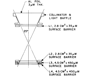
Figure 1: Cross-section of a LET telescope (adapted from Stone et al., 1977). Nominal areas and thicknesses of the detectors are shown in the figure. The 25^∘ half-angle of the field of view shown is for the more typical analysis condition, in which the first two detectors must trigger. In the analysis used here during the magrols, only the L1 detector is required to trigger. The nominal distance between the entrance window and L1 is 1.524 cm and the nominal radius of the window is 1.7695 cm, resulting in an 121^∘ full acceptance angle for the particles.

The CRS data from the magrols consist of counting rates of particles triggering the first detector in a stack of four detectors that make up a LET telescope. The cross-section of a LET is shown in Figure 1. There are four LETs on each of the Voyager spacecraft, referred to as LETs A, B, C, and D. They are identical in design, differing in practice only by small differences in the characteristics of the nominally identical detectors and in the slightly different component spacings and positionings upon assembly. The particles dominating the L1 rates are protons with $\sim$0.5-35 MeV and a median energy of $\sim$1.3 MeV that enter through the collimator opening at the top. Additional information about the L1 rates can be found in Appendix A.

The four telescopes have their boresights arranged in a quasi-orthogonal manner. LETs A and C are mounted back-to-back and LETs B and D are mounted with their boresights orthogonal to each other and to LETs A and C (Stone et al., 1977).

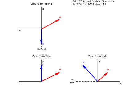
Figure 2: Three views showing the LET A and D telescope boresight unit vectors. The arrows indicate the viewing directions of the central axis of the telescope boresights.

Soon after the V2 encounter with Jupiter in 1979, the LET B telescope ceased returning data and the L1 detector of LET C was judged to have been implanted by sulfur and oxygen ions, creating a thin layer, $\sim$2.9 $\mu$ Si equivalent thickness, that is insensitive or partially insensitive to particles passing through it. This dead layer is believed to be slowly annealing (Breneman, 1985). To be sure this effect does not disturb the anisotropy results, and in particular the new radial component analysis, we have elected to use only LETs A and D, omitting LET C data from the analysis.

In Figure 2 we show the R, T, and N components of the unit vectors representing the LET A and D boresights in three views. The data are shown for 2011 day 117, which is representative to within $\sim$2^∘ for any time in the heliosheath when the spacecraft is not undergoing a maneuver. Looking at the view-from-the-Sun diagram, the projection of the LET D boresight onto the N-T plane is initially positioned at very near 0^∘, with the N axis serving as the origin of the angle measurement. The roll about the R axis is counter-clockwise in this view. The roll will advance the two LET boresights in N-T angle and an anisotropy of the cosmic-ray intensity in the N-T plane will be revealed if it is large enough.

The other important view in Figure 2 is the one from the side, which shows that the boresight of LET D has a negative R-component, whereas the boresight of LET A has a positive R-component. Thus, the R-component of the anisotropy vector can be determined if the relative responses of LETs A and D are known accurately enough.

In Figure 3 we show the counting rate from the LET A L1 detector (mostly protons with $\sim$0.5-35 MeV) during a typical 10-revolution roll maneuver on day 298 of 2011. The observed periodic variation is consistent with a first-order anisotropy with a period corresponding to the 2000 second duration of one 360^∘ revolution of the spacecraft.

In Figure 4 we show the data from both the LET A and LET D L1 detectors from the same roll as in Figure 3 but displayed as a function of roll angle rather than time. For all the rolls, LET A was in a command state such that the counting rate from L1 was one that has L4 in anti-coincidence (see Figure 1). LET D was in that same command state for the data shown in Figure 4, but that was not true for all magrols. For the rolls before 2011/258 and for the roll on 2014/254, the anti-coincidence term was not present and the rate was sampled only 1/16 of the time, whereas in the other command state the rate is continuously measured. We call the configuration in which LET D is in the statistically less favorable command state, configuration 1, and when LET D was in the same command state as LET A the configuration is referred to as configuration 2.

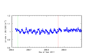
Figure 3: Counting rate of mostly protons with $\sim$0.5-35 MeV from the LET A L1 detector (in anti-coincidence with the L4 detector (see Stone et al., 1977)) during ten spacecraft rolls on day 298 of 2011. The symbols are 5-point moving averages, where a point represents data collected over a 48-second time period. The vertical green line marks the start of the roll and the vertical red line marks the end of the roll.

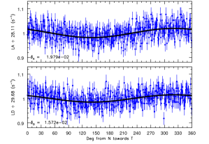
Figure 4: (top panel) Counting rate from LET A L1 detector in the L1$\overline{\textrm{L4}}$ command state from the magrol on day 298 of 2011 vs. angle from the N axis towards the T axis. The solid line represents the fit to a first-order anisotropy function as described in the text. The value of the anisotropy amplitude for the LET A data, $\delta_{A}$, derived from the fit is shown in the figure. (bottom panel) Same as top panel except for LET D.

Also shown in Figure 4 are the results of a simultaneous least-squares fit to a first-order anisotropy function to the rates in each telescope:

$$J_{A}=J_{0}(1+\vec{\delta}\cdot\vec{A})+Abkg$$ (1)

and

$$J_{D}=k_{D}J_{0}(1+\vec{\delta}\cdot\vec{D})+Dbkg$$ (2)

where $\vec{A}$, for example, refers to the unit vector that represents the boresight of LET A and $k_{D}$ represents the response normalization factor for LET D that accounts for the slightly non-identical geometry and response function to those of LET A. The quantities $Abkg$ and $Dbkg$ represent a background rate that is assumed isotropic. The method used to calculate these background rates is described in Appendix B.

The rates in Figure 4 are plotted versus angle in the N-T plane and thus the equations that are used in the fitting are written to accommodate that situation. For example, let $\beta_{A}$ represent the angle of the LET A boresight from N towards T in the N-T plane. This angle advances 8.64^∘ for each 48 s data point and is known based on the original boresight vector, the start time of the roll, and the roll rate. Let $\theta_{A}$ be the fixed angle of the LET A boresight vector from the R axis. Then, the components of the LET A boresight vector are $A_{R}=\cos\theta_{A}$, $A_{T}=\sin\theta_{A}\sin\beta_{A}$, and $A_{N}=\sin\theta_{A}\cos\beta_{A}$. Similar considerations apply to LET D. The fit parameters are $J_{0}$ and the R, T, and N components of the anisotropy vector, $\vec{\delta}$, with the normalization factor $k_{D}$ being determined as described below.

The R component of $\vec{\delta}$ depends critically on the factor $k_{D}$. In principle, this factor can be calculated by using a Monte Carlo simulation. We have done such a calculation, which not only provides an estimate of $k_{D}$ but also provides the C-G factor (Forman, 1970) that will be needed to convert between anisotropy vector components and solar wind speed components. We describe obtaining the C-G factor first.

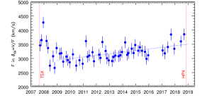
Figure 5: Compton-Getting factor for converting a solar wind velocity component to an anisotropy component as described in the text. For reference, an E^-1.5 spectrum gives F = 3303 km s^-1 from the Monte Carlo simulation for LET A. The dotted line was used to estimate the uncertainty on each point.

The C-G anisotropy, $\vec{\delta_{CG}}$, is given by

$$\vec{\delta_{CG}}=<(2-2\gamma)/v>\vec{V}$$ (3)

where $v$ is particle speed, $\vec{V}$ is the solar wind velocity, and $\gamma$ is the power-law index in the differential energy spectrum, dJ/dE $\sim$ E^γ, and the brackets $<>$ denote the average over the energy spectrum of the enclosed quantity. We have fit the energy spectra data to a four-power-law function for each roll day (or an adjacent roll day if the roll day had poor statistics) and then employed a Monte Carlo simulation using that function from 0.4-40 MeV to select particles and input them on the top of the aluminum window of a telescope. See Appendix A for an example of the resulting energy loss distribution in an L1 detector and how it compares with the observed distribution. The Monte Carlo simulation routine uses the same proton range-energy formulation that is used in other parts of the analysis of CRS data (Cook, 1981) and keeps track of whether energy losses in each detector exceed their threshold for triggering. One result of the simulation for the LET A telescope is the reciprocal of the coefficient of $\vec{V}$ in equation 3, which we show in Figure 5. An uncertainty of 204 km s^-1 on each point was derived by assuming the linear function shown by the dotted line represents the data from 2009 forward and by adjusting the uncertainty on each point to give a reduced $\chi^{2}$ = 1.0.

As mentioned, another result of the Monte Carlo simulation is the factor $k_{D}$, which is found by comparing the rates triggering the LET A and LET D L1 detectors in their appropriate command states for the same input energy spectrum, which itself varies somewhat over time and/or distance in the heliosheath. We found this calculation resulted in $k_{D}$ factors that were too small to make the converted radial solar wind speed, VR, agree with the PLS and LECP results when those two instruments agreed. This is likely due to incomplete knowledge of the exact areas of the detectors and collimator and/or spacings between telescope elements and their positionings that determine the effective geometrical factor of each telescope. The variation of the calculated $k_{D}$ factors over the 55 magrols in the heliosheath was small, typically much less than 1%. The variation is due to a slight dependence of the effective geometrical factor on the shape of the energy spectrum.

Our approach to this problem was to first do a series of fits in which the R-component of the anisotropy vector was fixed to be the value expected from the radial solar wind speed at the time of the roll and was obtained from the PLS measurements. We then picked normalization rolls, when PLS and LECP results for VR were in agreement; three when LET D was in the same command state as LET A (configuration 2; both in the L1$\overline{\textrm{L4}}$ mode) and three when LET D was in the L1 mode (configuration 1). The agreement between PLS and LECP for VR was determined from Figure 6 of Richardson & Decker (2014). The following rolls were used as normalizers for $k_{D}$ for configuration 1 (year/day of start of roll): 2008/73, 2008/114, 2008/353. For configuration 2, the normalization rolls were on 2013/73, 2013/164, and 2013/302. In each case the average of the $k_{D}$ from the simulation was compared to that from the $k_{D}$ that would result in a VR that would agree with PLS results (and LECP results). An average factor was determined that could be applied to the $k_{D}$ from the simulation to get the $k_{D}$ as a function of the rolls to use in a new set of fits, in which the R-component of the anisotropy vector was now a fit parameter. The two factors were 1.04294 for configuration 1 and 1.03106 for configuration 2. The resulting $k_{D}$ is shown in Figure 6.

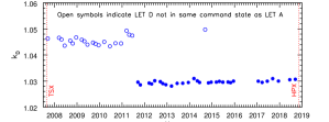
Figure 6: Normalization factor $k_{D}$ as a function of time that was used in fitting Equation 2 as described in the text. The solid symbols indicate rolls when LET A and D were in the same command state (configuration 2). The open symbols denote the $k_{D}$ for configuration 1.

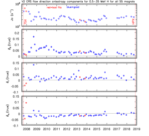
Figure 7: (top panel) Parameter $J_{0}$ from fits described in the text for 55 magrols when V2 was in the inner heliosheath. The red points represent fits that were judged to be not good by a $\chi^{2}$ test. The 51 blue points represent rolls that resulted in good fits. (second panel) Values of the R-component of the anisotropy amplitude from the fits. The designation “true” is described in the text. (third panel) Same as second panel except for the T-component of the anisotropy amplitude. (bottom panel) Same as third panel except for the N-component of the anisotropy amplitude. The vertical lines mark the times of the termination shock crossing (TSX) and the heliopause crossing (HPX).

We note that the counting rates that result from an anisotropy in the intensity of particles depends on the geometry of the telescope. The effect of the 121^∘ field of view was addressed in a Space Radiation Lab Internal Report #84 (1981) by N. Gehrels and D. Chenette (available upon request). From the internal report, it can be inferred that the reduction factor of the amplitude of the $\vec{\delta}$ that exists in space is the ratio of two integrals [$2\pi\int_{0}^{\pi}A(\theta)sin\theta cos\theta d\theta]/[2\pi\int_{0}^{\pi}A(\theta)sin\theta d\theta$] where $A(\theta)$ is the overlap area of two co-aligned, circular disks as a function of angle from the boresight axis and is given by Equation 10 of Sullivan (1971). According to the internal report, for the nominal LET telescope geometry, the reduction factor would be 3.8744/4.5964 = 0.8429. For the actual geometry of V2 LET A, we calculate the reduction factor to be 3.9573/4.7203 = 0.8384, which is the value used here.

In addition, we note that the $\vec{\delta}$ from the fits represents the direction from which the particles are coming. Thus, to represent the results for the actual flow direction and to correct for the 121^∘ field of view of the telescopes, we have multiplied the components from the fits by a factor of -1/0.8384 = -1.193 and labeled them as “true” in Figure 7. Also, the radial component has been increased in $\delta$ by the equivalent of 15 km s^-1, the spacecraft radial speed, to move the results out of the spacecraft frame of reference into the Sun frame. The figure shows the results for $J_{0}$ and the true R, T, and N components of $\vec{\delta}$ for all 55 magrols that occurred between the V2 crossing of the TS on 30 August 2007 and its crossing of the heliopause on 5 November 2018. The four rolls that were judged not to yield good fits by the Q statistic test are shown as red symbols in Figure 7. The results for the 51 good-fit rolls are shown in tabular form in Appendix C. Note that in the tables we have numbered the rolls using our own system in which roll 1 was on day 123 of 2001.

3 Radial Component of Solar Wind Velocity

The derivation of the radial component of the anisotropy vector during magrols for $\sim$0.5-35 MeV protons from CRS observations is a new development. As noted earlier, this radial component can be converted to the convective radial solar wind speed, VR, using the C-G method (Forman, 1970). The observations for VR from CRS, along with those from PLS and LECP, are shown in Figure 8. Except for one CRS very high value in 2008 (from magrol 46 on day 255 of 2008), which represents an unusual streaming event that will be the subject of a future study, there is remarkable agreement between the CRS and LECP results, including for the previously discounted 2009.3-2010.5 period (period A in Richardson & Decker (2014)). Yet, the CRS and LECP inferred speeds are often different from the directly measured speeds from PLS. We note that because of the agreement between CRS and LECP during 2009.3-2010.5, it now appears that oxygen ions were not contaminating the LECP data during that period.

Figure 8: (top panel) Radial component of the solar wind velocity from CRS (blue), PLS (green), and LECP (red). LECP (5-day averages) and CRS data (for all 51 good-fit rolls) are derived values based on the C-G effect. PLS data are daily averages and are direct measurements. The six periods used to normalize the LET D to LET A rates are shown as the solid circles. The LECP data are from a combination of data presented in Richardson & Decker (2014) and Richardson et al. (2020). (bottom panel) Daily-averaged LET A L1$\overline{\textrm{L4}}$ rate ($\sim$0.5-35 MeV protons). Starting in mid-2012, most of the increases in this rate align with increases in the LECP VR values. The dotted vertical lines are drawn to illustrate the correlation. These LET A L1$\overline{\textrm{L4}}$ rate increases are indicators of pressure pulses discussed in Richardson et al. (2018). During the quieter times between the pressure pulses, the LECP and CRS VR values are significantly below the actual measured VR values from PLS.

Just after the termination shock crossing, for a period of about 1 year, all three instruments gave approximately the same results for VR. Then, there is the afore-mentoned period from $\sim$2009.3-2010.5, when the CRS and LECP values were much higher than those directly measured by PLS, by as much as a factor of $\sim$2.5. Starting soon after that, the inferred radial solar wind speeds from LECP appeared to oscillate, at first on average near the PLS measurements, which were not oscillating, and then they trended down to below the PLS measurements as V2 moved closer to the heliopause.

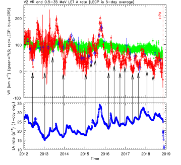
Figure 9: Same as Figure 8 except for time period shown and the vertical scales have been changed. The arrows show the correspondence of the local minima in the LET A L1$\overline{\textrm{L4}}$ rate and the local minima in the LECP inferred radial solar wind speeds.

Richardson et al. (2018) describe possible pressure waves in the heliosheath at V2. The counting rate of $\sim$0.5-35 MeV protons track these pressure changes and this rate is shown in the bottom panel of Figure 8. We note that after $\sim$mid-2012 there appears to be a good correlation of local maxima in this rate with local maxima in the VR from LECP and CRS.

If one were to consider only the lower pressure regions, the LECP data would show VR values near zero as the heliopause was approached, similar to that which was observed at V1. This is shown more clearly in Figure 9, where the arrows show the correspondence of the local minima in the $\sim$0.5-35 MeV rate with the local minima in the LECP and CRS VR speeds. However, the PLS VR values did not approach zero but were near 80 km s^-1 during that time. This finding then calls into question the stagnation region reported as V1 approached the heliopause, which was based on the V1 LECP inferences of VR using the C-G effect that showed VR trending towards zero as the heliopause was approached (Krimigis et al., 2011).

We do not understand why there is such good agreement, in general, between CRS and LECP VR results during times when PLS is different. Ordinarily, if the C-G method gives the same result at two different energies, not to mention two widely different energy bands as we have here, it would be confirmation that the correct solar wind speed had been deduced. But, that is apparently not the case with these measurements.

If the differences are attributed to the presence of a diffusive particle flow, the agreement between CRS and LECP for VR would imply an R component of the diffusive particle flow vector that differs at 28-43 keV versus that at $\sim$0.5-35 MeV by the ratio of their C-G factors, which would be 3303/513 = 6.4 for an E^-1.5 spectrum. The diffusive anisotropy depends on particle speed, $v$, the diffusion tensor, $K$, and the gradient of the number density per unit energy, $U$ (Forman, 1970) according to:

$$\vec{\delta_{\rm{diff}}}=-(3/v)K\cdot\bigtriangledown U/U$$ (4)

Near the heliopause, where the C-G-derived radial speeds are below those of PLS, the diffusive flow would need to be directed inwards to explain the observations.

The Monte Carlo simulations revealed that the typical median energy for the $\sim$0.5-35 MeV interval is $\sim$1.3 MeV (see Appendix A). So, the factor of $\sim$6.4 described above would imply an $\sim$$E^{-0.5}$ energy dependence to the product of the factors in Equation 4. The study of this phenomenon is deferred to the future.

4 Summary

We have used data from CRS acquired during occasional rolls of the V2 spacecraft when V2 was in the inner heliosheath and deduced the radial, tangential, and normal components of the anisotropy flow vector for $\sim$0.5-35 MeV protons. The measurement of the radial component of the anisotropy vector is a new development for CRS data. We have converted those radial components into radial solar wind speeds using the C-G method and compared with results from LECP, derived in a similar way, and also with the direct measurements from PLS.

We find that there is more than one aspect to the comparisons. There is an initial period of $\sim$1 year after the termination shock crossing when all three instruments give approximately the same results, except for one CRS result in 2008 that deserves a separate study. That is followed by a period of $\sim$1.2 years, the period A in Richardson & Decker (2014), when the C-G-derived results from LECP and CRS agree with each other, but are much higher, up to a factor of $\sim$2.5 times higher, than the direct measurements from PLS. We do not offer an explanation for this difference. However, we note that Richardson & Decker (2014) speculated that the LECP measurements during period A may have been contaminated by oxygen ions. The new inferences of VR from CRS are key to ruling out this explanation and point to an unexplained phenomenon at work.

After $\sim$mid-2012, beginning approximately five years after the termination shock crossing, there is a remarkable correlation between pressure pulses, characterized by changes in the plasma density and particle intensities, and variations in the CRS and LECP C-G-derived radial solar wind speeds. Often these speeds do not agree with the direct measurements from PLS. In the low pressure regions the LECP VR values trend towards zero, similar to the phenomenon that was seen at V1. However, PLS on V2 did not observe a real trend of VR towards zero across the heliosheath. Thus, the question is raised about whether the trend in VR inferred by LECP at V1 was a real trend of the radial solar wind speed or not.

While it is plausible that the solar wind might stagnate somewhere in the outer heliosphere, the fact that the V1 magnetic field strength did not increase proportionally argues against it happening along the V1 trajectory. The assertion that there is a stagnation region was made by instruments on V1 that used the C-G method to infer the solar wind speeds. There is no working plasma instrument on V1 with which to make direct measurements. Now we have the situation on V2 where the C-G method used by two instruments using very different energy ranges are getting the same VR, but they are not always in agreement with the direct measurements from the working plasma instrument on V2. In particular, in the vicinity of the heliopause at V2, even the average of the oscillatory VR inferred from LECP observations using the C-G method is significantly below the VR from PLS and trends downwards with time. Also, the values during the minima of the C-G VR oscillations are near zero km s^-1, while PLS is measuring radial speeds near 80 km s^-1.

Assuming the PLS speeds are correct, some phenomenon is interfering with the C-G method’s ability to give the correct radial speeds, at least at V2. And the interference is in such a way that CRS at $\sim$0.5-35 MeV and LECP at 28-43 keV are getting the same incorrect answer. If this same phenomenon is operating along V1’s trajectory through the inner heliosheath, then the implication is that there is no stagnation region before the heliopause at V1.

The trends toward zero speeds across the heliosheath at both V1 and V2 for the other two components, $\delta_{T}$ and $\delta_{N}$, have been addressed previously (Stone & Cummings, 2011; Stone et al., 2017; Cummings et al., 2019) and the results suggest that a diffusive flow of ACRs is responsible, at least in the case of $\delta_{T}$. Updates of those studies, based on the new techniques outlined in this work for CRS, are planned for the future.

Appendix A Characteristics of the  0.5-35 MeV Rate

Several quantities of interest to this investigation rely on a Monte Carlo code written to simulate the response of the L1 detectors to an input energy spectrum. In this Appendix, we show some of the results from the Monte Carlo program.

The code uses a range vs. energy relationship for protons in Si that was used in other parts of the analysis of CRS data (see, e.g., Cook (1981) and Cook et al. (1984)). A proton with an energy randomly selected from a differential energy spectrum, in the range from 0.4-40 MeV, and with a random trajectory selected from an isotropic angular distribution, is input at a random position on the front Al window (see Figure 1). The particle is followed along a straight-line trajectory and intersections with any detectors are noted. Energy loss in each detector layer is calculated and compared to the threshold energy for triggering that detector and that information is used in determining how many successful triggers occurred for various coincidence conditions.

The model of the LET telescope used in the simulation includes information on vertical detector spacings noted during their assembly, as well as thicknesses and areas of the detectors determined from pre-launch measurements. The average thicknesses of the two front detectors, L1 and L2, were measured prior to launch in five concentric rings, each 2 mm in width, using radioactive sources, and those data are incorporated into the simulations.

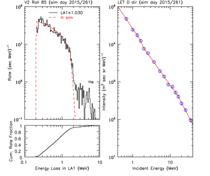
Figure 10: (top right) Incident energy spectrum of protons appropriate for the LET D direction for day 261 of 2015. The observations (open circles) are from CRS. The red line is a fit of the data to a four-power-law function that is used as input to the Monte Carlo simulation program described in the text. (top left) Energy-loss distribution in LET A L1 detector for the L1$\overline{\textrm{L4}}$ coincidence condition from the simulation (dashed red line) along with the observed energy-loss distribution (histogram). Above $\sim$2 MeV the observed distribution is dominated by He ions. (lower left) Cumulative fraction of the rate vs. energy loss in LET A L1.

In Figure 10 we show both an input energy spectrum and the resulting energy loss distribution in LET A L1 for the coincidence condition L1$\overline{\textrm{L4}}$, which was the only coincidence condition for LET A used in this work. The incident energy spectrum was measured by CRS and is for 2015/261, which is the day after the actual magrol (number 85). It is often necessary for statistical reasons to use a day adjacent to the actual day of the magrol for the simulations. The input to the Monte Carlo program is the four-power-law fit to the data shown in the right panel.

The four lowest-energy data points of the input energy spectrum are from analysis of the observed energy-loss measurements shown in the left panel of the figure, after corrections for background. These four points have been corrected to be as if they were from LET D by a factor determined by the relative counting rates of LET A L1 and LET D L1. This was necessary because the LET A multi-detector data, used for the next five highest-energy points, have very poor statistics, and LET D was used for these. The remaining points are from the High-Energy Telescope ( HET) 1. More information about the multi-detector data analysis can be found in Cummings et al. (2016).

Since the measured energy spectrum and the simulation are appropriate for the LET D direction, the observed energy loss distribution from LET A L1$\overline{\textrm{L4}}$, shown in the top left panel, has been multiplied by a factor to account for that difference. The factor is taken from Figure 6 and the procedure describing how it was obtained is described in the text.

The simulated energy-loss distribution and the observed energy-loss distribution are in good agreement below $\sim$2 MeV. Above that energy, the observed energy-loss distribution is dominated by He ions. (See Stone & Cummings (2003) for simulations using He and heavier ions.) Based on the lower left panel of Figure 10, $\sim$95% of the rate responds to protons. The He ions are anomalous cosmic rays and would be expected to have similar anisotropy characteristics to those of the protons, so they are not treated as background. Rather, the anisotropy study in this work is regarded as pertaining to a population of particles dominated by protons with $\sim$0.5-35 MeV.

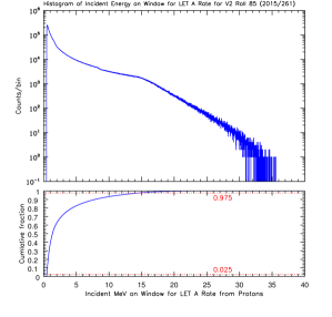
Figure 11: (top) Histogram of the incident energies for the same simulation used to produce the results shown in Figure 10. Incident protons above $\sim$35 MeV at the extreme allowable angle to the normal deposit too little energy in L1 to trigger the threshold of the L1 detector. Incident protons below $\sim$0.5 MeV are also unable to trigger the threshold. (bottom) Cumulative counts of the distribution shown in the top panel vs. incident energy expressed as a fraction of the total. The two horizontal dotted lines indicate that 95% of the distribution is from $\sim$0.5-14 MeV.

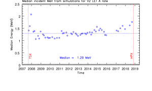
Figure 12: Median incident energies from the distributions like those in Figure 11 for all 55 magrols vs. time.

In Figure 11 we show the histogram of incident energies that resulted in LET A L1$\overline{\textrm{L4}}$ triggers for the same simulation used in Figure 10. It is apparent why the energy interval ascribed to the L1 rates is $\sim$0.5-35 MeV. However, as shown in the lower panel, $\sim$95% of the rate is due to protons with $\sim$0.5-14 MeV.

Another way to characterize the incident energy distribution is to cite the median energy. For the distribution shown in Figure 11 the median energy is 1.36 MeV. In Figure 12 we show the median energies for all 55 magrols used in this work. While there is a trend upward in the medians due to the evolving incident energy spectra with time, the median of the medians is 1.29 MeV. Thus the $\sim$0.5-35 MeV rate can also be considered as a rate of $\sim$1.3 MeV protons. This characterization of this rate is only appropriate when the energy spectra are similar to the shape they have in the heliosheath.

Appendix B Estimation of GCR Background

When V2 crossed the heliopause on day 309 of 2018, the counting rates from the detectors used in this study gradually dropped from $\sim$25 s^-1 at the time of the crossing to $\sim$2 s^-1 at and beyond day 10 of 2019 (Stone et al., 2019). This decline represented the effect of the ACRs escaping into the VLISM. The residual counting rate of $\sim$2 s^-1 represents a background due to galactic cosmic rays. To estimate this background rate as a function of time, we used a high-energy GCR rate (named PENL) from the HET 2 telescope and correlated it with the L1 rates during times we believe all the rate is due to this GCR background source.

The correlation for LET D L1 rate is shown in Figure 13. The blue curve represents the background formula that was used for Dbkg in Equation 2: $\textrm{Dbkg}=3.8\textrm{PENL}-0.0915$. LET D was typically in the L1-only command state (configuration 1). In some cases, denoted as configuration 2, it was put into the L1$\overline{\textrm{L4}}$ command state just before a magrol and then returned to the configuration 1 state just after the roll ended. Thus, since this correlation with the PENL rate was only done for configuration 1, for configuration 2 we adjusted the Dbkg value by the ratio of the rates obtained during those rolls, L1$\overline{\textrm{L4}}$/L1.

The correlation for LET A L1$\overline{\textrm{L4}}$ with the PENL rate is shown in Figure 14. LET A was permanently put into the command state L1$\overline{\textrm{L4}}$ in 2000, so only the time after that is available for the correlation. The blue curve in the top panel is the result of the equation $\textrm{Abkg}=3.6\textrm{PENL}-0.124$ and this was used in the fits to Equation 1. The background counting rates for all 55 magrols are shown in Figure 15.

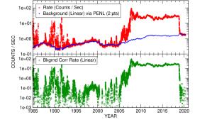
Figure 13: (top panel) Counting rate of LET D L1 detector vs. time. Also shown as the blue points are the estimated GCR background rates based on the PENL rate as described in the text. (bottom panel) LET D L1 rate corrected for GCR background.

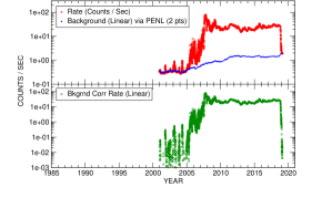
Figure 14: Same as Figure 13 except for the LET A L1$\overline{\textrm{L4}}$ rate.

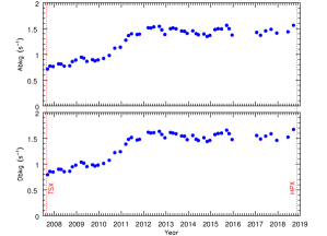
Figure 15: The background counting rates, Abkg and Dbkg in Equations 1 and 2, for all 55 magrols in the heliosheath.

Appendix C Tables of Parameters

Table 1: Results from anisotropy fits for all good-fit rolls for 0.5-35 MeV protons

Roll	Year	Day	Jo	$\delta_{R}$ (true)	$\delta_{T}$ (true)	$\delta_{N}$ (true)	$k_{D}$	Abkg	Dbkg	F
40	2007	256	46.43 $\pm$ 0.08	1.82e-02 $\pm$ 4.7e-03	2.88e-02 $\pm$ 1.9e-03	-1.98e-02 $\pm$ 1.9e-03	1.04630	0.7155	0.7946	3458.3
43	2008	73	45.27 $\pm$ 0.13	3.46e-02 $\pm$ 8.0e-03	1.87e-02 $\pm$ 3.4e-03	-2.29e-02 $\pm$ 3.4e-03	1.04659	0.8150	0.8997	3617.8
44	2008	114	35.65 $\pm$ 0.06	3.45e-02 $\pm$ 5.3e-03	1.28e-03 $\pm$ 2.3e-03	-2.64e-02 $\pm$ 2.3e-03	1.04595	0.8121	0.8966	3366.5
45	2008	165	17.14 $\pm$ 0.05	7.08e-02 $\pm$ 7.9e-03	4.14e-03 $\pm$ 3.3e-03	-2.86e-02 $\pm$ 3.3e-03	1.04358	0.7711	0.8534	2744.2
46	2008	255	19.89 $\pm$ 0.05	1.65e-01 $\pm$ 7.3e-03	1.30e-01 $\pm$ 3.0e-03	2.50e-02 $\pm$ 3.0e-03	1.04550	0.7785	0.8612	3077.5
47	2008	297	27.25 $\pm$ 0.07	9.89e-02 $\pm$ 6.2e-03	2.32e-02 $\pm$ 2.6e-03	-1.33e-02 $\pm$ 2.5e-03	1.04439	0.8591	0.9462	2663.2
48	2008	353	26.45 $\pm$ 0.07	4.50e-02 $\pm$ 7.8e-03	3.36e-02 $\pm$ 3.2e-03	-2.34e-02 $\pm$ 3.2e-03	1.04674	0.8898	0.9787	3364.4
49	2009	78	42.68 $\pm$ 0.07	5.91e-02 $\pm$ 5.0e-03	3.09e-02 $\pm$ 2.1e-03	2.01e-02 $\pm$ 2.1e-03	1.04584	0.9459	1.0379	3170.6
50	2009	119	27.44 $\pm$ 0.07	6.75e-02 $\pm$ 6.1e-03	-1.30e-02 $\pm$ 2.6e-03	-1.32e-02 $\pm$ 2.6e-03	1.04528	0.9267	1.0175	3184.2
51	2009	170	21.82 $\pm$ 0.06	6.83e-02 $\pm$ 6.9e-03	9.84e-03 $\pm$ 2.9e-03	-2.02e-02 $\pm$ 2.9e-03	1.04394	0.8637	0.9511	2884.5
52	2009	260	22.83 $\pm$ 0.06	7.32e-02 $\pm$ 6.8e-03	1.39e-02 $\pm$ 2.8e-03	-3.19e-02 $\pm$ 2.8e-03	1.04473	0.8970	0.9863	3063.2
53	2009	300	22.44 $\pm$ 0.06	7.46e-02 $\pm$ 7.0e-03	-4.68e-03 $\pm$ 2.8e-03	-4.20e-02 $\pm$ 2.8e-03	1.04428	0.8742	0.9622	2941.1
54	2009	351	20.53 $\pm$ 0.06	8.62e-02 $\pm$ 7.3e-03	3.86e-03 $\pm$ 3.0e-03	-3.75e-02 $\pm$ 3.0e-03	1.04374	0.8913	0.9802	2863.1
55	2010	77	20.55 $\pm$ 0.06	5.31e-02 $\pm$ 7.1e-03	9.87e-03 $\pm$ 3.0e-03	-2.39e-02 $\pm$ 3.0e-03	1.04503	0.9217	1.0123	3143.2
56	2010	169	19.68 $\pm$ 0.05	7.78e-02 $\pm$ 7.3e-03	1.98e-02 $\pm$ 3.1e-03	-2.26e-02 $\pm$ 3.1e-03	1.04335	0.9800	1.0738	2744.3
57	2010	259	23.16 $\pm$ 0.06	5.21e-02 $\pm$ 6.8e-03	3.53e-02 $\pm$ 2.8e-03	-2.25e-02 $\pm$ 2.8e-03	1.04450	1.1197	1.2213	2935.2
58	2010	350	18.50 $\pm$ 0.05	3.99e-02 $\pm$ 7.7e-03	2.37e-02 $\pm$ 3.2e-03	-2.95e-02 $\pm$ 3.2e-03	1.04443	1.1384	1.2411	2811.0
59	2011	74	21.98 $\pm$ 0.06	2.90e-02 $\pm$ 7.7e-03	1.14e-03 $\pm$ 3.3e-03	-2.49e-02 $\pm$ 3.3e-03	1.04930	1.2762	1.3864	3611.1
60	2011	117	26.95 $\pm$ 0.08	2.70e-02 $\pm$ 7.1e-03	1.35e-02 $\pm$ 3.0e-03	-1.29e-02 $\pm$ 3.0e-03	1.04776	1.3646	1.4798	3056.7
61	2011	167	29.71 $\pm$ 0.07	3.71e-02 $\pm$ 5.9e-03	2.76e-02 $\pm$ 2.5e-03	-1.28e-02 $\pm$ 2.5e-03	1.04744	1.3993	1.5164	3101.7
62	2011	258	28.49 $\pm$ 0.03	3.01e-02 $\pm$ 2.2e-03	1.18e-02 $\pm$ 2.0e-03	-2.33e-02 $\pm$ 2.0e-03	1.02955	1.3857	1.4669	3216.9
63	2011	298	26.99 $\pm$ 0.03	3.36e-02 $\pm$ 2.2e-03	1.62e-02 $\pm$ 2.1e-03	-2.01e-02 $\pm$ 2.1e-03	1.02852	1.3920	1.4803	2898.9
64	2012	75	25.34 $\pm$ 0.03	3.66e-02 $\pm$ 2.3e-03	7.58e-03 $\pm$ 2.2e-03	-1.78e-02 $\pm$ 2.2e-03	1.02922	1.5160	1.6167	3131.6
65	2012	116	22.46 $\pm$ 0.02	2.72e-02 $\pm$ 2.4e-03	7.36e-03 $\pm$ 2.3e-03	-1.27e-02 $\pm$ 2.3e-03	1.02889	1.5112	1.6037	3018.5
66	2012	167	20.24 $\pm$ 0.02	1.17e-02 $\pm$ 2.6e-03	2.59e-02 $\pm$ 2.4e-03	-3.37e-03 $\pm$ 2.4e-03	1.03011	1.5318	1.6092	3579.1

Note. — Roll number created for purposes of this paper; units of Jo are s^-1; date information is for start of roll; true refers to direction of flow in the Sun frame and corrected for wide field of view of telescope; units of Abkg and Dbkg are s^-1; F is C-G factor in units of km s^-1 with estimated uncertainty of 204 km s^-1.

Table 2: Results from anisotropy fits for all good-fit rolls for 0.5-35 MeV protons (continued)

Roll	Year	Day	Jo	$\delta_{R}$ (true)	$\delta_{T}$ (true)	$\delta_{N}$ (true)	$k_{D}$	Abkg	Dbkg	F
67	2012	257	20.37 $\pm$ 0.02	2.66e-02 $\pm$ 2.6e-03	5.02e-02 $\pm$ 2.4e-03	-1.82e-02 $\pm$ 2.4e-03	1.02975	1.5438	1.6326	3263.7
68	2012	297	17.71 $\pm$ 0.03	2.83e-02 $\pm$ 2.8e-03	1.08e-02 $\pm$ 2.6e-03	-1.40e-02 $\pm$ 2.6e-03	1.02903	1.4750	1.5744	3005.4
69	2012	348	15.26 $\pm$ 0.05	3.09e-02 $\pm$ 7.3e-03	2.88e-02 $\pm$ 7.1e-03	-1.16e-02 $\pm$ 6.8e-03	1.02859	1.3854	1.5095	2932.1
70	2013	73	14.91 $\pm$ 0.03	3.06e-02 $\pm$ 3.1e-03	8.03e-02 $\pm$ 3.0e-03	-8.37e-03 $\pm$ 3.0e-03	1.02806	1.4982	1.6124	2907.7
72	2013	164	18.16 $\pm$ 0.03	2.46e-02 $\pm$ 2.7e-03	3.25e-03 $\pm$ 2.6e-03	-1.94e-02 $\pm$ 2.6e-03	1.02910	1.4958	1.5865	3101.0
73	2013	255	17.99 $\pm$ 0.03	3.35e-02 $\pm$ 2.8e-03	9.76e-03 $\pm$ 2.6e-03	-2.31e-02 $\pm$ 2.6e-03	1.02915	1.4529	1.5449	3077.4
75	2013	346	15.14 $\pm$ 0.02	2.75e-02 $\pm$ 3.0e-03	2.32e-02 $\pm$ 2.8e-03	-7.21e-03 $\pm$ 2.8e-03	1.02944	1.4068	1.4732	3227.3
76	2014	72	19.77 $\pm$ 0.02	3.23e-02 $\pm$ 2.6e-03	1.42e-02 $\pm$ 2.5e-03	-1.83e-02 $\pm$ 2.5e-03	1.03095	1.4563	1.5556	3565.2
77	2014	127	19.01 $\pm$ 0.02	4.28e-02 $\pm$ 2.7e-03	2.10e-02 $\pm$ 2.5e-03	-1.57e-02 $\pm$ 2.5e-03	1.03005	1.4013	1.4807	3125.9
78	2014	163	17.72 $\pm$ 0.03	3.70e-02 $\pm$ 2.8e-03	3.61e-02 $\pm$ 2.6e-03	-1.88e-02 $\pm$ 2.6e-03	1.02945	1.3808	1.4583	3189.5
79	2014	254	17.95 $\pm$ 0.05	3.05e-02 $\pm$ 8.0e-03	1.04e-02 $\pm$ 3.3e-03	-1.96e-02 $\pm$ 3.3e-03	1.04973	1.3948	1.5117	3343.9
80	2014	307	16.67 $\pm$ 0.03	1.53e-02 $\pm$ 2.9e-03	2.21e-02 $\pm$ 2.7e-03	-1.49e-02 $\pm$ 2.7e-03	1.02929	1.3487	1.4392	3191.7
81	2014	352	16.41 $\pm$ 0.03	1.36e-02 $\pm$ 2.9e-03	1.22e-02 $\pm$ 2.7e-03	-1.42e-02 $\pm$ 2.7e-03	1.02956	1.3676	1.4600	3474.0
82	2015	70	20.71 $\pm$ 0.02	1.71e-02 $\pm$ 2.5e-03	1.49e-02 $\pm$ 2.4e-03	-1.43e-02 $\pm$ 2.4e-03	1.02959	1.4799	1.5735	3272.8
83	2015	119	19.05 $\pm$ 0.02	1.00e-02 $\pm$ 2.7e-03	2.07e-02 $\pm$ 2.5e-03	-1.19e-02 $\pm$ 2.5e-03	1.02985	1.4970	1.5927	3393.0
84	2015	176	21.54 $\pm$ 0.02	2.06e-02 $\pm$ 2.5e-03	2.10e-02 $\pm$ 2.3e-03	-1.49e-02 $\pm$ 2.3e-03	1.02957	1.4918	1.6001	3267.9
85	2015	260	29.81 $\pm$ 0.03	4.11e-02 $\pm$ 2.1e-03	1.20e-02 $\pm$ 2.0e-03	-4.67e-03 $\pm$ 2.0e-03	1.02962	1.5620	1.6571	3233.4
86	2015	300	27.86 $\pm$ 0.03	5.50e-02 $\pm$ 2.2e-03	6.62e-02 $\pm$ 2.0e-03	1.64e-02 $\pm$ 2.0e-03	1.02938	1.4984	1.5914	2985.0
87	2015	349	23.10 $\pm$ 0.02	3.66e-02 $\pm$ 2.4e-03	1.54e-02 $\pm$ 2.2e-03	-1.54e-02 $\pm$ 2.3e-03	1.02996	1.3743	1.4762	3111.2
88	2017	20	23.58 $\pm$ 0.08	3.00e-02 $\pm$ 7.9e-03	4.00e-02 $\pm$ 7.5e-03	2.13e-03 $\pm$ 7.6e-03	1.02993	1.4260	1.5529	3282.1
89	2017	83	23.38 $\pm$ 0.06	2.10e-02 $\pm$ 5.3e-03	3.05e-02 $\pm$ 5.1e-03	2.82e-03 $\pm$ 5.1e-03	1.02948	1.3705	1.4855	3180.0
90	2017	166	25.29 $\pm$ 0.06	1.64e-02 $\pm$ 5.1e-03	1.65e-02 $\pm$ 4.8e-03	-9.61e-03 $\pm$ 4.8e-03	1.02993	1.4554	1.5423	3401.7
91	2017	254	24.83 $\pm$ 0.06	3.46e-03 $\pm$ 5.2e-03	3.73e-02 $\pm$ 4.9e-03	-2.97e-03 $\pm$ 4.9e-03	1.03092	1.4868	1.5866	3844.9
92	2017	348	28.33 $\pm$ 0.08	1.86e-02 $\pm$ 5.3e-03	-1.68e-03 $\pm$ 4.9e-03	-1.26e-02 $\pm$ 5.1e-03	1.02998	1.4135	1.4601	3340.9
93	2018	166	27.07 $\pm$ 0.07	1.83e-02 $\pm$ 5.0e-03	2.42e-02 $\pm$ 4.7e-03	7.25e-03 $\pm$ 4.7e-03	1.03052	1.4375	1.5228	3601.1
94	2018	256	25.82 $\pm$ 0.07	1.09e-02 $\pm$ 5.1e-03	6.14e-03 $\pm$ 4.8e-03	2.97e-03 $\pm$ 4.8e-03	1.03066	1.5634	1.6714	3853.0

References

- Breneman (1985) Breneman, H. H. 1985, PhD thesis, California Institute of Technology, Pasadena.
- Bridge et al. (1977) Bridge, H. S., Belcher, J. W., Butler, R. J., et al. 1977, Space Sci. Rev., 21, 259, doi: 10.1007/BF00211542
- Burlaga & Ness (2012) Burlaga, L. F., & Ness, N. F. 2012, ApJ, 749, 13, doi: 10.1088/0004-637X/749/1/13
- Cook (1981) Cook, W. R., I. 1981, PhD thesis, California Institute of Technology, Pasadena.
- Cook et al. (1984) Cook, W. R., Stone, E. C., & Vogt, R. E. 1984, ApJ, 279, 827, doi: 10.1086/161953
- Cummings et al. (2019) Cummings, A., Stone, E., Heikkila, B. C., Lal, N., & Richardson, J. 2019, in International Cosmic Ray Conference, Vol. 36, 36th International Cosmic Ray Conference (ICRC2019), 1071
- Cummings et al. (2016) Cummings, A. C., Stone, E. C., Heikkila, B. C., et al. 2016, ApJ, 831, 18, doi: 10.3847/0004-637X/831/1/18
- Decker et al. (2012) Decker, R. B., Krimigis, S. M., Roelof, E. C., & Hill, M. E. 2012, Nature, 489, 124, doi: 10.1038/nature11441
- Drake et al. (2017) Drake, J. F., Swisdak, M., Opher, M., & Richardson, J. D. 2017, ApJ, 837, 159, doi: 10.3847/1538-4357/aa6304
- Forman (1970) Forman, M. A. 1970, Planet. Space Sci., 18, 25, doi: 10.1016/0032-0633(70)90064-4
- Fränz & Harper (2002) Fränz, M., & Harper, D. 2002, Planet. Space Sci., 50, 217, doi: 10.1016/S0032-0633(01)00119-2
- Kane et al. (1998) Kane, M., Decker, R. B., Mauk, B. H., & Krimigis, S. M. 1998, J. Geophys. Res., 103, 267, doi: 10.1029/97JA02776
- Krimigis et al. (1977) Krimigis, S. M., Armstrong, T. P., Axford, W. I., et al. 1977, Space Sci. Rev., 21, 329, doi: 10.1007/BF00211545
- Krimigis et al. (2013) Krimigis, S. M., Decker, R. B., Roelof, E. C., et al. 2013, Science, 341, 144, doi: 10.1126/science.1235721
- Krimigis et al. (2011) Krimigis, S. M., Roelof, E. C., Decker, R. B., & Hill, M. E. 2011, Nature, 474, 359, doi: 10.1038/nature10115
- Opher et al. (2012) Opher, M., Drake, J. F., Velli, M., Decker, R. B., & Toth, G. 2012, ApJ, 751, 80, doi: 10.1088/0004-637X/751/2/80
- Pogorelov et al. (2012) Pogorelov, N. V., Borovikov, S. N., Zank, G. P., et al. 2012, ApJ, 750, L4, doi: 10.1088/2041-8205/750/1/L4
- Pogorelov et al. (2017) Pogorelov, N. V., Heerikhuisen, J., Roytershteyn, V., et al. 2017, ApJ, 845, 9, doi: 10.3847/1538-4357/aa7d4f
- Press et al. (1992) Press, W. H., Teukolsky, S. A., Vetterling, W. T., & Flannery, B. P. 1992, Numerical recipes in C. The art of scientific computing
- Richardson et al. (2020) Richardson, J. D., Belcher, J. W., Burlaga, L. F., et al. 2020, in IOP Conference Series, Vol. tbd, From the Sun’s Atmosphere to the Edge of the Galaxy: A Story of Connections: 19th Annual International Astrophysics Conference, ed. G. P. Zank, tbd, doi: 10.1088/1742-6596/1620/1/012016, 2020
- Richardson et al. (2018) Richardson, J. D., Belcher, J. W., Cummings, A. C., Decker, R., & Stone, E. C. 2018, in Journal of Physics Conference Series, Vol. 1100, Journal of Physics Conference Series, 012019, doi: 10.1088/1742-6596/1100/1/012019
- Richardson et al. (2013) Richardson, J. D., Burlaga, L. F., Decker, R. B., et al. 2013, ApJ, 762, L14, doi: 10.1088/2041-8205/762/1/L14
- Richardson & Decker (2014) Richardson, J. D., & Decker, R. B. 2014, Astrophys. J., 792, 126, doi: 10.1088/0004-637X/792/2/126
- Stone et al. (2017) Stone, E., Cummings, A. C., Heikkila, B. C., Lal, N., & Webber, W. R. 2017, International Cosmic Ray Conference, 301, 57
- Stone & Cummings (2003) Stone, E. C., & Cummings, A. C. 2003, in International Cosmic Ray Conference, Vol. 7, International Cosmic Ray Conference, 3781
- Stone & Cummings (2011) Stone, E. C., & Cummings, A. C. 2011, International Cosmic Ray Conference, 12, 29, doi: 10.7529/ICRC2011/V12/I06
- Stone et al. (2019) Stone, E. C., Cummings, A. C., Heikkila, B. C., & Lal, N. 2019, Nature Astronomy, 3, 1013, doi: 10.1038/s41550-019-0928-3
- Stone et al. (1977) Stone, E. C., Vogt, R. E., McDonald, F. B., et al. 1977, Space Sci. Rev., 21, 355
- Sullivan (1971) Sullivan, J. D. 1971, Nuclear Instruments and Methods, 95, 5, doi: 10.1016/0029-554X(71)90033-4