Equivariant Learning of Stochastic Fields:
Gaussian Processes and Steerable Conditional Neural Processes

Abstract

Motivated by objects such as electric fields or fluid streams, we study the problem of learning stochastic fields, i.e. stochastic processes whose samples are fields like those occurring in physics and engineering. Considering general transformations such as rotations and reflections, we show that spatial invariance of stochastic fields requires an inference model to be equivariant. Leveraging recent advances from the equivariance literature, we study equivariance in two classes of models. Firstly, we fully characterise equivariant Gaussian processes. Secondly, we introduce Steerable Conditional Neural Processes (SteerCNPs), a new, fully equivariant member of the Neural Process family. In experiments with Gaussian process vector fields, images, and real-world weather data, we observe that SteerCNPs significantly improve the performance of previous models and equivariance leads to improvements in transfer learning tasks.

1 Introduction

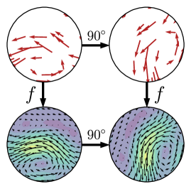
Figure 1: A schematic of equivariant learning of vector fields. The model $f$ predicts a vector field from a set of vectors (red arrows). It is equivariant to the action of rotations, here a 90^∘ rotation.

In physics and engineering, fields are objects which assign a physical quantity to every point in space. They serve as a unifying concept for objects such as electro-magnetic fields, gravity fields, electric potentials or fluid dynamics and are therefore omnipresent in the natural sciences and their applications (Landau, 2013). Our goal in this work is to be able to predict the value of a field everywhere given some finite set of observations (see $f$ in fig. 1). We will be interested in cases where these fields are not fixed but are drawn from a random distribution, which we term stochastic fields.

Viewing fields as usual mathematical functions, we can consider stochastic fields as stochastic processes. A well-known example of these are Gaussian processes (GPs) (Rasmussen & Williams, 2005) which have been widely used in machine learning. More recently, Neural Processes (NPs) and their related models were introduced as an alternative to GPs which enable to learn a stochastic process from data leveraging the flexibility of neural networks (Garnelo et al., 2018a, b; Kim et al., 2019).

When applying models to data from the natural sciences, it is a logical step to integrate scientific knowledge about the problem into these models. The physical principle of homogeneity of space states that all positions and orientations in space are equivalent, i.e. there is no canonical orientation or absolute position. A natural modelling assumption stemming from this is that the prior we place over a random field should be invariant, i.e. it should look the same from all positions and orientations. We will show that this implies that the posterior as a function of the observed points is equivariant.

Figure 1 illustrates this equivariance. The input is a discrete set of vectors at certain points in space, the red arrows, and the predictions a continuous vector field. If the space is homogenous, we would expect the predictions of a model to rotate in the same way as we rotate the data, i.e. we expect the model to be equivariant.

Translation equivariance in Gaussian processes has long been studied via stationary kernels. We extend this notion to derive Gaussian processes that are equivariant to more general transformations such as rotations and reflections. Recent work has also shown how to build translation equivariance into NP models (Gordon et al., 2020; Bruinsma et al., 2021). We will build on this work to introduce a new member of the Neural Process family that has more general equivariance properties. We do this utilising recent developments in equivariant deep learning (Weiler & Cesa, 2019). Imposing equivariance on deep learning models reduces the number of model parameters and has been shown to allow models to learn from data more efficiently (Cohen & Welling, 2016; Dieleman et al., 2016; Kondor & Trivedi, 2018). We will show that the same rational applies to NP models.

More specifically, our main contributions are as follows:

1. We show that stochastic process models are equivariant if and only if the underlying prior is spatially invariant - giving a natural criteria when such models are useful.

2. We find sufficient and necessary constraints for a vector-valued Gaussian process over $\mathbb{R}^{n}$ to be equivariant allowing the simple construction of equivariant GPs.

3. As a new, equivariant member of the Neural Process family, we present Steerable Conditional Neural Processes (SteerCNPs) and show that they outperform previous models on synthetic and real data.

2 Transforming Fields

We aim to build to a model which learns functions $F$ of the form $F:\mathbb{R}^{n}\to\mathbb{R}^{d}$. We call $F$ a (steerable) feature map since we interpret $F$ geometrically as mapping $n$-dimensional coordinates $\mathbf{x}\in\mathbb{R}^{n}$ to some $d$-dimensional feature $F(\mathbf{x})$. As intuitively clear from fig. 1, we should be able to rotate such a feature map as we do with an ordinary geographical map or an image. In this section, we make this rigorous using group theory (see appendix A for a brief introduction).

In the following, let $E(n)$ be the group of isometries on $\mathbb{R}^{n}$. Let $T(n)$ be the group of translations of $\mathbb{R}^{n}$ which can be identified with $\mathbb{R}^{n}$. $T(n)$ acts from the left on $\mathbb{R}^{n}$ via $t_{\mathbf{x}}(\mathbf{x}^{\prime})=\mathbf{x}^{\prime}+\mathbf{x}$ for all $\mathbf{x},\mathbf{x}^{\prime}\in\mathbb{R}^{n}$. Let $O(n)$ be the group of $n\times n$ orthogonal matrices, acting from the left on $\mathbb{R}^{n}$ by matrix multiplication. We write $SO(n)$ for the subgroup of rotations, i.e. elements $A\in O(n)$ with $\det A=1$.

We describe all possible transformations of a feature map $F$ by a subgroup $G\subset E(n)$. We assume that $G$ is the semidirect product of $T(n)$ and a subgroup $H$ of $O(n)$, i.e. every $g\in G$ is a unique composition of a translation $t_{\mathbf{x}}$ and an orthogonal map $h\in H$:

$$g=t_{\mathbf{x}}h$$ (1)

As common, we call $H$ the fiber group. Depending on the inference problem, one would often pick $H=SO(n)$ or $H=O(n)$ (equivalently $G=SE(n),E(n)$). However, using finite subgroups $H$ can be more computationally efficient, and give better empirical results (Weiler & Cesa, 2019). In particular, in dimension $n=2$ we use the Cyclic groups $C_{m}$, comprised of the rotations by $\frac{k2\pi}{m}$ ($k=0,1,\dots,m-1$) and the dihedral group $D_{m}$ containing $C_{m}$ combined with reflections.

To describe transformations of a feature map $F$ via a group $G$, we need a linear representation $\rho:H\to\text{GL}(\mathbb{R}^{d})$ of $H$ which we call fiber representation. The action of $G$ on a steerable feature map $F$ is then defined as

$$g.F(\mathbf{x})=\rho(h)F(g^{-1}\mathbf{x})$$ (2)

where $g=t_{\mathbf{x}^{\prime}}h\in G$. Figure 2 demonstrates for vector fields why the transformation defined here is a sensible notion to consider. In group theory, this is called the induced representation of $H$ on $G$ denoted by $\text{Ind}_{H}^{G}\rho$.

In allusion to physics, we use the term (steerable) feature field referring to the feature map $F:\mathbb{R}^{n}\to\mathbb{R}^{d}$ together with its corresponding law of transformation given by $\rho$ (Weiler & Cesa, 2019). We write $\mathcal{F}_{\rho}$ for the space of these fields. Typical examples are:

1. Scalar fields $F:\mathbb{R}^{n}\to\mathbb{R}$ have trivial fiber representation $\rho=\rho_{triv}$, i.e. $\rho(h)=\mathbf{1}$ for $h\in H$, such that

   $$g.F(\mathbf{x})=F(g^{-1}\mathbf{x})$$ (3)

   Examples are greyscale images or temperature maps.

2. Vector fields $F:\mathbb{R}^{n}\to\mathbb{R}^{n}$ have $\rho=\rho_{\text{Id}}$, i.e. $\rho(h)=h$ for $h\in H$, such that

   $$g.F(\mathbf{x})=hF(g^{-1}\mathbf{x})$$ (4)

   Examples include electric fields or wind maps.

3. Stacked fields: given fields $F_{1},\dots,F_{n}$ with fiber representations $\rho_{1},\dots,\rho_{n}$ we can stack them to $F=(F_{1},\dots,F_{n})$ with fiber representation as the direct sum $\rho=\rho_{1}\oplus\cdots\oplus\rho_{n}$. Examples include a combined wind and temperature map or RGB-images.

Finally, for simplicity we assume that $\rho$ is an orthogonal representation, i.e. $\rho(h)\in O(d)$ for all $h\in H$. Since all fiber groups $H$ of interest are compact, this is not a restriction (Serre, 1977).

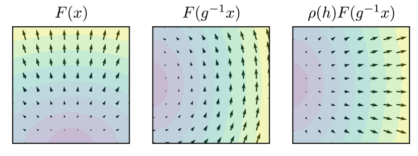
Figure 2: Demonstration of the transformation of vector fields on $\mathbb{R}^{2}$ under the action of $g=t_{\mathbf{x}^{\prime}}h\in G=SE(2)=\mathbb{R}^{2}\rtimes SO(2)$. Color represents the norm of a vector at each point.

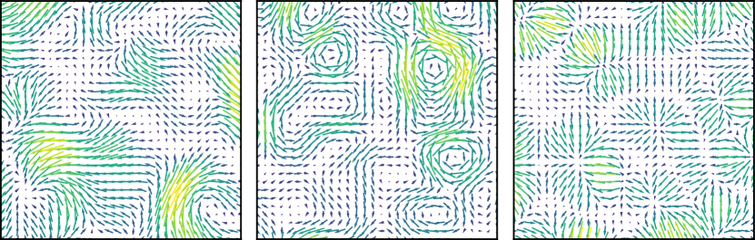
(a)

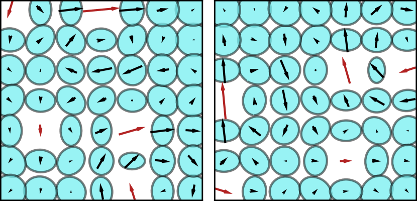
(b)

Figure 3: (a) GP-samples of $2d$-vector fields from different $E(2)$-equivariant kernels. Left: RBF-kernel. Middle: divergence-free kernel. Right: curl-free kernel. (b) Illustration of theorem 1. Left: posterior GP means (black) and confidence ellipses (blue) from data (red). Right: posterior given rotated data. One can see that means and confidence ellipses rotate with the data.

3 Equivariant Stochastic Process Models

In this work, we are interested in learning not only a single feature field $F$ but a probability distribution $P$ over $\mathcal{F}_{\rho}$, i.e. a stochastic process over feature fields $F$. For example, $P$ could describe the distribution of all wind maps over a specific region. If $F\sim P$ is a random feature field and $g\in G$, we can define the transformed stochastic process $g.P$ as the distribution of $g.F$. We say that $P$ is $G$-invariant if

$$P=g.P\quad\text{for all }g\in G$$ (5)

From a sample $F\sim P$, our model observes only a finite set of input-output pairs $Z=\{(\mathbf{x}_{i},\mathbf{y}_{i})\}_{i=1}^{n}$ where $\mathbf{y}_{i}$ equals $F(\mathbf{x}_{i})$ plus potentially some noise. The induced representation naturally translates to a transformation of $Z$ under $G$ via

$$g.Z:=\{(g\mathbf{x}_{i},\rho(h)\mathbf{y}_{i})\}_{i=1}^{n}$$ (6)

In a Bayesian approach, we can consider $P$ as a prior and given an observed data set $Z$ we can consider the posterior, i.e. the conditional distribution $P_{Z}$ of $F$ given $Z$. As the next proposition shows, equivariance of the posterior is the other side of the coin to invariance of the prior.

Proposition 1.

Let $P$ be a stochastic process over $\mathcal{F}_{\rho}$. Then $P$ is $G$-invariant if and only if the posterior map $Z\mapsto P_{Z}$ is $G$-equivariant, i.e.

$$P_{g.Z}=g.P_{Z}\quad\text{for all }g\in G$$ (7)

The proof of this can be found in section B.1.

In most real-world scenarios, it may not be possible to exactly compute the posterior and our goal is to build a model $Q$ which returns an approximation $Q_{Z}$ of $P_{Z}$. However, often it is our prior belief that the distribution $P$ is $G$-invariant. Given proposition 1, it is then natural to construct an approximate inference model $Q$ which is itself equivariant.

We will see applications of these ideas to GPs and CNPs in sections 4 and 5.

4 Equivariant Gaussian Processes

A widely-studied example of stochastic processes are Gaussian processes (GPs). Here we will look at Gaussian processes under the lens of equivariance. Since we are interested in vector-valued functions $F:\mathbb{R}^{n}\to\mathbb{R}^{d}$, we use matrix-valued positive definite kernels $K:\mathbb{R}^{n}\times\mathbb{R}^{n}\to\mathbb{R}^{d\times d}$ (Álvarez et al., 2012).

In the case of GPs, we assume that for every $\mathbf{x},\mathbf{x}^{\prime}\in\mathbb{R}^{n}$, it holds that $F(\mathbf{x})$ is normally distributed with mean $\mathbf{m}(\mathbf{x})$ and covariances $\text{Cov}(F(\mathbf{x}),F(\mathbf{x}^{\prime}))=K(\mathbf{x},\mathbf{x}^{\prime})$. We write $\mathcal{GP}(\mathbf{m},K)$ for the stochastic process defined by this.

We can fully characterise all mean functions and kernels leading to equivariant GPs:

Theorem 1.

A Gaussian process $\mathcal{GP}(\mathbf{m},K)$ is $G$-invariant, equivalently the posterior $G$-equivariant, if and only if

1. $\mathbf{m}(\mathbf{x})=\mathbf{m}\in\mathbb{R}^{d}$ is constant with $\mathbf{m}$ such that

   $$\rho(h)\mathbf{m}=\mathbf{m}\quad\text{for all }h\in H$$ (8)

2. $K$ fulfils the following two conditions:

   1. $K$ is stationary, i.e. for all $\mathbf{x},\mathbf{x}^{\prime}\in\mathbb{R}^{n}$

      $$K(\mathbf{x},\mathbf{x}^{\prime})=K(\mathbf{x}-\mathbf{x}^{\prime},\mathbf{0})=:\hat{K}(\mathbf{x}-\mathbf{x}^{\prime})$$ (9)

   2. $K$ satisfies the angular constraint, i.e. for all $\mathbf{x},\mathbf{x}^{\prime}\in\mathbb{R}^{n},h\in H$ it holds that

      $$K(h\mathbf{x},h\mathbf{x}^{\prime}) =\rho(h)K(\mathbf{x},\mathbf{x}^{\prime})\rho(h)^{T}$$ (10)

      or equivalently, for all $\mathbf{x}\in\mathbb{R}^{n},h\in H$

      $$\hat{K}(h\mathbf{x}) =\rho(h)\hat{K}(\mathbf{x})\rho(h)^{T}$$ (11)

   If this is the case, we call $K$ $\rho$-equivariant.

The proof of this can be found in section B.2.

We note the distinct similarity between the kernel conditions in eqs. 9 and 10, and the ones found in the equivariant convolutional neural network literature (see for example eq. (2) in Weiler & Cesa (2019)). In contrast to convolutional kernels, we have the additional constraint that the kernel $K$ must be positive definite.

A popular example to model vector-valued functions is to simply use $d$ independent GPs with a stationary scalar kernel $k:\mathbb{R}^{n}\to\mathbb{R}$. This leads to a kernel $K(\mathbf{x})=k(\mathbf{x})I$ which can easily be seen to be $E(n)$-equivariant.

As a non-trivial example of equivariant kernels, we will also consider the divergence-free and curl-free kernels (see appendix C) used in physics introduced by Macêdo & Castro (2010) which allow us to model divergence-free and curl-free fields such as electric or magnetic fields (see fig. 3(a) for examples).

We note that the kernels considered in this work represent a small set of possible kernels permitted by theorem 1. Much of the standard Gaussian Process and kernel machinery, e.g. Bochner’s theorem, random Fourier features (Brault et al., 2016), and sparse methods, extend naturally to the vector-valued and equivariant case.

5 Steerable Conditional Neural Processes

Conditional Neural Processes were introduced as an alternative model to Gaussian processes. While GPs require us to explicitly model the prior $P$ and can perform exact posterior inference, CNPs aim to learn an approximation to the posterior map ($Z\mapsto P_{Z}$) directly, only implicitly learning a prior from data. Generally speaking, the underlying architecture is a model which returns a mean function $\mathbf{m}_{Z}:\mathbb{R}^{n}\to\mathbb{R}^{d}$ and a covariance function $\mathbf{\Sigma}_{Z}:\mathbb{R}^{n}\to\mathbb{R}^{d\times d}$ given a context set $Z$. For simplicity, it makes the assumption that given $Z$ the functions values $F(\mathbf{x})$ are conditionally independent and normally distributed

$$F(\mathbf{x})\sim\mathcal{N}(\mathbf{m}_{Z}(\mathbf{x}),\mathbf{\Sigma}_{Z}(\mathbf{x})),\quad F(\mathbf{x})\perp\!\!\!\perp F(\mathbf{x}^{\prime})\;|\;Z$$ (12)

Let us call a model as in eq. 12 a conditional process model. As we did with $F\in\mathcal{F}_{\rho}$, we can specify a law of transformation by considering $\mathbf{m}_{Z}$ as a mean feature field in $\mathcal{F}_{\rho_{m}}$ and $\mathbf{\Sigma}_{Z}$ as a covariance feature field in $\mathcal{F}_{\rho_{\Sigma}}$ for appropriate fiber representations $\rho_{m},\rho_{\Sigma}$. With this, we can easily characterise equivariance in conditional process models:

Proposition 2.

A conditional process model is $G$-equivariant if and only if the mean and covariance feature maps are $G$-equivariant, i.e. it holds for all $g\in G$ and context sets $Z$

$$\mathbf{m}_{g.Z} =g.\mathbf{m}_{Z}$$ (13)

$$\mathbf{\Sigma}_{g.Z} =g.\mathbf{\Sigma}_{Z}$$ (14)

with $\rho_{m}=\rho$ and $\rho_{\Sigma}=\rho\otimes\rho$ the tensor product with action given by

$$\rho_{\Sigma}(h)A=\rho(h)A\rho(h)^{T},\quad A\in\mathbb{R}^{d\times d}$$ (15)

The proof can be found in section B.3.

In the following, we will restrict ourselves to perform inference from data sets of multiplicity $1$, i.e., data sets $Z=\{(\mathbf{x}_{i},\mathbf{y}_{i})\}_{i=1}^{m}$ where $\mathbf{x}_{i}\neq\mathbf{x}_{j}$ for all $i\neq j$. We denote the collection of all such data sets with $\mathcal{Z}_{\rho}$ meaning that they transform under $\rho$ (see eq. 6).

Moreover, we assume that there is no order in a data set $Z$, i.e. we aim to build models which are not only $G$-equivariant but also invariant to permutations of $Z$.

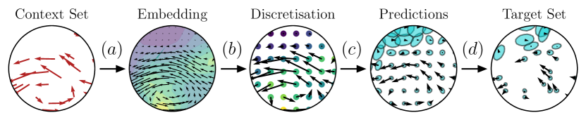
Figure 4: SteerCNP model illustration. (a) Embed the context set into a function. (b) Discretise this embedding on a regular grid. (c) Predict the mean and covariance of the conditional stochastic process on the grid of points. (d) Use kernel smoothing to predict the mean and covariance at target locations.

The following generalisation of the ConvDeepSets theorem of Gordon et al. (2020) gives us a universal form of all such conditional process models. We simple need to pick $\rho_{\text{in}}=\rho$ and $\rho_{\text{out}}=\rho_{m}\oplus\rho_{\Sigma}=\rho\oplus\rho_{\Sigma}$ in the following theorem.

Theorem 2 (EquivDeepSets).

Let $\rho_{\text{in}},\rho_{\text{out}}$ be the two fiber representations. Define the embedding representation as the direct sum $\rho_{E}=\rho_{triv}\oplus\rho_{\text{in}}$.
A function ${\Phi}:\mathcal{Z}_{\rho_{\text{in}}}\to\mathcal{F}_{\rho_{\text{out}}}$ is $G$-equivariant and permutation invariant if and only if it can be expressed as

$${\Phi}(Z)=\Psi(E(Z))$$ (16)

for all $Z=\{(\mathbf{x}_{i},\mathbf{y}_{i})\}_{i=1}^{m}\in\mathcal{Z}_{\rho_{\text{in}}}$ with

1. $E(Z)=\sum_{i=1}^{m}K(\cdot,\mathbf{x}_{i})\phi(\mathbf{y}_{i})$

2. $\phi(\mathbf{y})=(1,\mathbf{y})^{T}\in\mathbb{R}^{d+1}$.

3. $K:\mathbb{R}^{n}\times\mathbb{R}^{n}\to\mathbb{R}^{(d+1)\times(d+1)}$ is a $\rho_{E}$-equivariant strictly positive definite kernel (see theorem 1).

4. $\Psi:\mathcal{F}_{\rho_{E}}\to\mathcal{F}_{\rho_{\text{out}}}$ is a ${G}$-equivariant function.

Additionally, by imposing extra constraints (see section B.4), we can also ensure that $\Phi$ is continuous.

The proof of this can be found in appendix B.4. Using this, we can start to build SteerCNPs by building an encoder $E$ and a decoder ${\Psi}$ as specified in the theorem.

The form of the encoder only depends on the choice of a kernel $K$ which is equivariant under $\rho_{E}$. An easy but effective way of doing this is to pick a kernel $K_{0}$ which is equivariant under $\rho$ (see section 4) and a scalar kernel $k:\mathbb{R}^{n}\to\mathbb{R}$ and then use the block-version $K=k\oplus K_{0}$.

5.1 Decoder

By theorem 2, it remains to construct a $G$-equivariant decoder $\Psi$. To construct such maps, we will use steerable CNNs (Cohen & Welling, 2017; Weiler & Cesa, 2019; Weiler et al., 2018). In theory, a layer of such a network is an equivariant function $\Psi:\mathcal{F}_{\rho_{\text{in}}}\to\mathcal{F}_{\rho_{\text{out}}}$ where we are free to choose fiber representations $\rho_{\text{in}},\rho_{\text{out}}$.

Steerable convolutional layers are defined by a kernel $\kappa:\mathbb{R}^{n}\to\mathbb{R}^{c_{\text{out}}\times c_{\text{in}}}$ such that the map

$$[\kappa\star F](\mathbf{x})=\int\kappa(\mathbf{x},\mathbf{x}^{\prime})F(\mathbf{x}^{\prime})d\mathbf{x}$$ (17)

is $G$-equivariant. These layers serve as the learnable, parameterisable functions.

Steerable activation functions are applied pointwise to $F$. These are functions $\sigma:\mathbb{R}^{c_{\text{in}}}\to\mathbb{R}^{c_{\text{out}}}$ such that

$$\sigma(\rho_{\text{in}}(h)\mathbf{x})=\rho_{\text{out}}(h)\sigma(\mathbf{x})$$ (18)

As a decoder of our model, we use a stack of equivariant convolutional layers composed with equivariant activation functions. The convolutions in eq. 17 are computed in a discretised manner after sampling $E(Z)$ on a grid $\mathcal{G}\subset\mathbb{R}^{n}$. Therefore, the output of the neural network will be a discretised version of a function and we use kernel smoothing to extend the output of the network to the whole space.

5.2 Covariance Activation Functions

The output of a steerable neural network has general vectors in $\mathbb{R}^{c}$ for some $c$ as outputs. Therefore, we need an additional component to obtain (positive definite) covariance matrices in an equivariant way.

We introduce the following concept:

Definition 1.

An equivariant covariance activation function is a map $\eta:\mathbb{R}^{c}\to\mathbb{R}^{d\times d}$ together with a fiber representation $\rho_{\eta}:H\to\text{GL}(\mathbb{R}^{c})$ such that for all $\mathbf{y}\in\mathbb{R}^{c}$ and $h\in H$

1. $\eta(\mathbf{y})$ is a symmetric, positive semi-definite matrix.

2. $\eta(\rho_{\eta}(h)\mathbf{y})=\rho_{\Sigma}(h)\eta(\mathbf{y})$

In our case, we use a quadratic covariance activation function which we define by

$$\eta:\mathbb{R}^{d\times d}\to\mathbb{R}^{d\times d},\quad\eta(A)=AA^{T}$$

Considering $A=(a_{1},\dots,a_{D})\in\mathbb{R}^{d^{2}}$ as a vector by stacking the columns, the input representation is then $\rho_{\eta}=\rho\oplus\dots\oplus\rho$ as the $d$-times sum of $\rho$. It is straight forward to see that $\eta$ is equivariant and outputs positive semi-definite matrices.

5.3 Full model

Finally, we summarise the architecture of the SteerCNP (see fig. 4):

1. The encoder produces an embedding of a data set $Z$ as a function $E(Z)$.

2. A discretisation of $E(Z)$ serves as input for the decoder, a steerable CNN with input fiber representation $\rho_{E}$ and output fiber representation $\rho\oplus\rho_{\eta}$.

3. On the covariance part, we apply the covariance activation function $\eta$.

4. The grid values of the mean and the covariances are extended to the whole space $\mathbb{R}^{n}$ via kernel smoothing.

We train the model similar to the CNP by iteratively sampling a data set $Z$ and splitting it randomly in a context set $Z_{C}$ and a target set $Z_{T}$. The context set $Z_{C}$ is then passed forward through the SteerCNP model and the mean log-likelihood of the target $Z_{T}=\{(\mathbf{x}^{\prime}_{i},\mathbf{y}^{\prime}_{i})\}_{i=1}^{m}$ is computed. In brief, we minimise the loss

$$-\mathbb{E}_{Z_{C},Z_{T}\sim P}\left[\frac{1}{m}\sum\limits_{i=1}^{m}\log\mathcal{N}(\mathbf{y}_{i}^{\prime};\mathbf{m}_{Z_{C}}(\mathbf{x}^{\prime}_{i}),\mathbf{\Sigma}_{Z_{C}}(\mathbf{x}^{\prime}_{i}))\right]$$

by gradient descent methods.

In sum, this gives a CNP model, which up to discretisation errors is equivariant with respect to arbitrary transformations from the group $G$ and invariant to permutations.

6 Related Work

Equivariance and symmetries in deep learning. Motivated by the success of the translation-equivariant CNNs (LeCun et al., 1990), there has been a great interest in building neural networks which are equivariant also to more general transformations. Approaches use a wide range of techniques such as convolutions on groups (Cohen et al., 2018; Kondor & Trivedi, 2018; Cohen & Welling, 2016; Hoogeboom et al., 2018; Worrall & Brostow, 2018), cylic permutations (Dieleman et al., 2016), Lie groups (Finzi et al., 2020a) or phase changes (Worrall et al., 2016). It was in the context of Steerable CNNs and its various generalisations where ideas from physics about fields started to play a more prominent role. (Cohen & Welling, 2017; Weiler et al., 2018; Weiler & Cesa, 2019; Cohen et al., 2019). We use this framework since it allows for modelling of non-trivial transformations of features $F(\mathbf{x})$ via fiber representations $\rho$, as for example necessary to model transformations of vector fields (see eq. 4).

Gaussian Processes and Kernels. Classical GPs using kernels such as the RBF or Matérn kernels have been widely used in machine learning to model scalar fields (Rasmussen & Williams, 2005). Vector-valued GPs, which allow for dependencies across dimensions via matrix-valued kernels, were common models in geostatistics (Goovaerts et al., 1997) and also played a role in kernel methods (Álvarez et al., 2012). With this work, we showed that many of these GPs are equivariant (see theorem 1) giving a further theoretical foundation for their applicability. In contrast to equivariant GPs, Reisert & Burkhardt (2007) consider the construction of equivariant functions from kernels, arriving at similar equivariance constraints as we do in theorem 1.

Neural Processes. Garnelo et al. (2018a) introduced Conditional Neural Processes (CNPs) as an architecture constructed out of neural networks which learns an approximation of stochastic processes from data. They share the motivation of meta-learning methods (Finn et al., 2017; Andrychowicz et al., 2016) to learn a distribution of tasks instead of only a single task. Neural Processes (NPs) are the latent variable counterpart of CNPs allowing for correlations across the marginals of the posterior. Both CNPs and NPs have been combined with other machine learning concepts, for example attention mechanisms (Kim et al., 2019).

Gordon et al. (2020) were the first to consider symmetries in NPs. Inspired by the prevalence of stationary kernels in the GP literature, they introduced a translation-equivariant NP model, along with a universal characterisation of such models. Our work can be seen as a generalisation of their method. By picking a trivial fiber group $H=\{e\}$ and $K$ as a diagonal RBF-kernel in SteerCNPs (see theorem 2), we get the ConvCNP as a special case of SteerCNPs.

During the development of this work, Kawano et al. (2021) also studied more general equivariance in CNPs, restricting themselves to scalar fields and focusing on Lie Groups. They only compared their approach with previous models on $1d$ synthetic regression tasks where their approach did not seem to outperform ConvCNPs, and in this case the added symmetry is redundant. In contrast, we focus on general scalar and vector-valued fields with non-trivial transformations $\rho$. As we show in the next section, this ”steerable” approach leads to significant performance gains compared to previous models. The decomposition theorem presented in Kawano et al. (2021) can be seen as a special case of theorem 2 in this work by setting $\rho=\rho_{tri}$.

7 Experiments

Finally, we provide empirical evidence that equivariance is a helpful bias in stochastic process models. We focus on evaluating SteerCNPs since inference with the variety of GPs, which this work shows to be equivariant, has been studied exhaustively.

7.1 Gaussian Process Vector Fields

A common baseline task for CNPs is regression on samples from a Gaussian process (Garnelo et al., 2018a; Gordon et al., 2020), partially because one can directly compare the output of the model with the true posterior. Here, we consider the task of learning $2$D vector fields $F:\mathbb{R}^{2}\to\mathbb{R}^{2}$ which are samples of a Gaussian process $\mathcal{GP}(0,K)$ with 3 different $E(2)$-equivariant kernels $K$: the diagonal RBF-kernel, the divergence-free kernel and the curl-free kernel (see figs. 3(a) and C).

We run extensive experiments comparing the SteerCNP with the CNP and the translation-equivariant ConvCNP. On the SteerCNP, we impose various levels of rotation and reflection equivariance by picking different fiber groups $H$. As usual for CNPs, we use the mean log-likelihood as a measure of performance. The maximum possible log-likelihood is obtained by Monte Carlo sampling using the true GP posterior.

In table 1, the results are presented. Overall, one can see that the SteerCNP clearly outperforms previous models by reducing the difference to the GP baseline by more than a half. In addition, we observe that small fiber groups ($H=C_{4}$) lead to the best results. Although theoretically models with the largest fiber groups ($H=C_{16},SO(2)$) should perform better, it is possible that practical limitations such as discretisation of the model favors smaller fiber groups since they still allow for compensation of marginal asymmetries and numerical errors. For the case of $H=SO(2)$, the worse results are consistent with results from Weiler & Cesa (2019) in supervised learning and practical reasons for this are discussed in more depth there. Hence, we leave out $SO(2)$ in further experiments.

Table 1: Results for experiments on GP vector fields. Mean log-likelihood $\pm$ 1 standard deviation over 5 random seeds reported. Last row shows GP-baseline (optimum).

Model	RBF	Curl-free	Div-free
CNP	-4.24$\pm$0.00	-0.750$\pm$0.004	-0.752$\pm$0.006
ConvCNP	-3.88$\pm$0.01	-0.541$\pm$0.004	-0.533$\pm$0.001
SteerCNP ($SO(2)$)	-3.93$\pm$0.05	-0.550$\pm$0.005	-0.552$\pm$0.008
SteerCNP ($C_{4}$)	-3.66$\pm$0.00	-0.461$\pm$0.003	-0.464$\pm$0.007
SteerCNP ($C_{8}$)	-3.70$\pm$0.01	-0.479$\pm$0.004	-0.478$\pm$0.004
SteerCNP ($C_{16}$)	-3.71$\pm$0.02	-0.476$\pm$0.005	-0.480$\pm$0.008
SteerCNP ($D_{4}$)	-3.72$\pm$0.03	-0.471$\pm$0.002	-0.477$\pm$0.005
SteerCNP ($D_{8}$)	-3.68$\pm$0.03	-0.462$\pm$0.005	-0.467$\pm$0.008
GP	-3.50	-0.410	-0.411

7.2 Image in-painting

To test the SteerCNP on purely scalar data we evaluate our model on an image completion task. In image completion tasks the context set is made up of pairs of 2D pixel locations and pixel intensities and the objective is to predict the intensity at new locations. For further details see section D.3, along with qualitative results from the experiments.

MNIST and rotMNIST. We first train models on completion tasks from the MNIST data set (LeCun et al., 2010). The results in table 4 show that the equivariance built into the SteerCNP is useful, with the various SterableCNPs outperforming previous models. To test whether this performance gain could be replicated by data augmentation, we trained the models on a variant, called rotMNIST, produced by randomly rotating each digit in the dataset. We find that this does not improve results in the non equivariant models, in fact causing a decrease in performance as they try to learn a more complex distribution from too little data. It therefore seems to be the gain in parameter and data efficiency due the imposed equivariance constraints what leads to better performance of SteerCNPs.

Generalising to larger images. One key advantage of equivariant models is that they should be able to extrapolate to data at locations and orientations previously unseen. To test this, we create a new data set by sampling 2 rotMNIST images and randomly translating them in a 56*56 image, calling this dataset extMNIST (for extrapolate). We evaluate the models trained on MNIST on this data set. The results in table 4 show the significant benefit of the additional rotation equivariance.

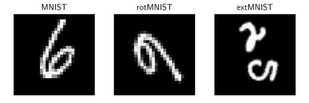
Figure 5: Examples of the three datasets

Table 2: Results for the MNIST experiments. Mean log-likelihood $\pm$ 1 standard deviation over 3 random model and dataset seeds reported.

Train dataset	MNIST	rotMNIST	MNIST
Test dataset	MNIST	MNIST	extMNIST
Model
GP	0.39$\pm$0.30	0.39$\pm$0.30	0.72$\pm$0.17
CNP	0.76$\pm$0.05	0.66$\pm$0.06	-1.11$\pm$0.06
ConvCNP	1.01$\pm$0.01	0.95$\pm$0.01	1.08$\pm$0.02
SteerCNP($C_{4}$)	1.05$\pm$0.02	1.02$\pm$0.03	1.14$\pm$0.02
SteerCNP($C_{8}$)	1.07$\pm$0.03	1.05$\pm$0.04	1.16$\pm$0.03
SteerCNP($C_{16}$)	1.08$\pm$0.03	1.04$\pm$0.03	1.17$\pm$0.05
SteerCNP($D_{4}$)	1.08$\pm$0.03	1.05$\pm$0.03	1.14$\pm$0.03
SteerCNP($D_{8}$)	1.08$\pm$0.03	1.04$\pm$0.04	1.17$\pm$0.02

7.3 ERA5 Weather Data

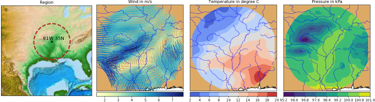
Figure 6: Illustration of ERA5 weather data from the US.

To evaluate the performance of the SteerCNP model on vector-valued fields, we retrieved weather data from the global ERA5 data set. We extracted data from a circular region surrounding Memphis, Tennessee, and from a region of the same size in Hubei province, Southern China (see fig. 6 for illustration and appendix D for details). While the specific choice of these areas was arbitrary, we tried to pick two topologically different regions far away from each other.

Every sample $F$ from these data sets corresponds to a weather map consisting of temperature, pressure and wind in the region at one single point in time. We give the models the task to infer a wind vector field from a data $Z$ of pairs $(\mathbf{x},\mathbf{y})$ where $\mathbf{y}=(y^{t},y^{p},y^{w}_{1},y^{w}_{2})\in\mathbb{R}^{4}$ gives the temperature, pressure and wind at point $\mathbf{x}$. In particular, the output features are only a subset of the input features. To deal with such a task, we can simply pick different input and output fiber representations for the SteerCNP:

$$\rho_{\text{in}}=\rho_{triv}\oplus\rho_{triv}\oplus\rho_{\text{Id}},\quad\rho_{\text{out}}=\rho_{\text{Id}}$$

Performance on US data. As a first experiment, we split the US data set in a train, validation and test data set. Then we train and test the models accordingly. We observe that the SteerCNP outperforms previous models like a GP with RBF-kernel, the CNP and the ConvCNP with a significant margin for all considered fiber groups (see table 3). Again, we observe that a relatively small fiber group $C_{4}$ leads to the best results. Inference from weather data is clearly not exactly equivariant due to local differences such as altitude and distance to the sea. Therefore, it seems that a SteerCNP model with small fiber groups like $C_{4}$ enables us to exploit the equivariant patterns much better than the ConvCNP and CNP but leaves flexibility to account for asymmetric patterns.

Generalising to a different region. As a second experiment, we take these models and test their performance on data from China. This can be seen as a transfer learning task. Intuitively, posing a higher equivariance restriction on the model makes it less adapting to special local circumstances and more robust when transferring to a new environment. Indeed, we observe that the CNP, the ConvCNP and the model with fiber group $C_{4}$ have a larger loss in performance than SteerCNP models with larger fiber groups such as $C_{16},D_{8},D_{4}$. Similarly, while GPs had a significantly worse performance than ConvCNPs on the US data, it outperforms it on the transfer to China data. In applications like robotics where environments constantly change this robustness due to equivariance might be advantageous.

Table 3: Results on ERA5 weather experiment trained on US data. Mean log-likelihood $\pm$ 1 standard deviation over 5 random seeds reported. Left: tested on US data. Right: tested on China data.

Model	US	China
GP	0.386$\pm$0.005	-0.755$\pm$0.001
CNP	0.001$\pm$0.017	-2.456$\pm$0.365
ConvCNP	0.898$\pm$0.045	-0.890$\pm$0.059
SteerCNP ($C_{4}$)	1.255$\pm$0.019	-0.578$\pm$0.173
SteerCNP ($C_{8}$)	1.038$\pm$0.026	-0.582$\pm$0.104
SteerCNP ($C_{16}$)	1.094$\pm$0.015	-0.550$\pm$0.073
SteerCNP ($D_{4}$)	1.037$\pm$0.037	-0.429$\pm$0.067
SteerCNP ($D_{8}$)	1.032$\pm$0.011	-0.539$\pm$0.129

8 Limitations and Future Work

Similar to CNPs, our model cannot capture dependencies between the marginals of the posterior. Recently, Foong et al. (2020) introduced a translation-equivariant NP model which allows to do this and future work could combine their approach with general symmetries considered in this work.

As stated earlier, our model works for Euclidean spaces of any dimension. The limiting factor is the development of Steerable CNNs used in the decoder. In our experiments, we focused on $\mathbb{R}^{2}$ as the code is well developed by Weiler & Cesa (2019). Recent developments in the design of equivariant neural networks also explore non-Euclidean spaces such as spheres and encourage exploration in this direction in the context of NPs (Cohen et al., 2019, 2018; Esteves et al., 2020). Additionally, in Euclidean space we can incorporate other symmetries such as scaling via Lie group approaches, similar to (Kawano et al., 2021), or symmetry to uniform motion for fluid flow (Wang et al., 2020) by choosing suitable equivariant CNNs.

One practical limitation of this method is the necessity to discretise the continuous RKHS embedding, which can be costly and breaks the theoretical guarentees found in this work in theorem 2. An alternative approach would be to move away entirely from the structure of theorem 2, and build an architecture more similar to the original CNP, utilising equivariant point cloud methods (Finzi et al., 2020b; Hutchinson et al., 2020; Satorras et al., 2021) to produce the embedding of the context set. This would avoid the discretisation of the embedding grid and may provide speedups, but looses the flexibility promised by theorem 2.

9 Conclusion

In this work, we considered the problem of learning stochastic fields and focused on using their geometric structure. We motivated the design of equivariant stochastic process models by showing the equivalence of equivariance in the posterior map to invariance in the prior data distribution. We fully characterised equivariant Gaussian processes and introduced Steerable Conditional Neural Processes, a model that combines recent developments in the design of equivariant neural networks with the family of Neural Processes. We showed that it improves results of previous models, even for data which shows inhomogeneities in space such as weather, and is more robust to perturbations in the underlying distribution.

Our work shows that implementing general symmetries in stochastic process or meta-learning models could be a substantial step towards more data-efficient and adaptable machine learning models. Inference models which respect the structure of fields, in particular vector fields, could further improve the application of machine learning in natural sciences, engineering and beyond.

Acknowledgements

Peter Holderrieth is supported as a Rhodes Scholar by the Rhodes Trust. Michael Hutchinson is supported by the EPSRC Centre for Doctoral Training in Modern Statistics and Statistical Machine Learning (EP/S023151/1). Yee Whye Teh’s research leading to these results has received funding from the European Research Council under the European Union’s Seventh Framework Programme (FP7/2007-2013) ERC grant agreement no. 617071.

We would also like to thank the Python community (Van Rossum & Drake Jr, 1995; Oliphant, 2007) for developing the tools that enabled this work, including Pytorch (Paszke et al., 2017b), NumPy (Oliphant, 2006; Walt et al., 2011; Harris et al., 2020), SciPy (Jones et al., 2001), and Matplotlib (Hunter, 2007).

Appendix A Basics for Group and Representation Theory

This section gives the basic definitions about groups and representations necessary to understand this work. We refer to the literature for a more detailed introduction (Artin, 2011; Bröcker & Dieck, 2003).

A.1 Groups

A group $(G,\cdot)$ is a set $G$ together with a function $\cdot:G\times G\to G,(g,h)\mapsto g\cdot h$ called group operation satisfying

1. (Associativity): $g\cdot(h\cdot i)=(g\cdot h)\cdot i$ for all $g,h,i\in G$

2. (Existence of a neutral element): There is a $e\in G$ such that: $e\cdot g=g\cdot e=g$ for all $g\in G$

3. (Existence of an inverse): For all $g\in G$, there is a $g^{-1}$ such that $e=g^{-1}\cdot g=g\cdot g^{-1}$

If in addition, $G$ satisfies

1. (Commutativity): $g\cdot h=h\cdot g$ for all $g,h\in G$

$G$ is called Abelian. We simply write $g_{1}g_{2}$ for $g_{1}\cdot g_{2}$ if it is clear from the context.

If $\rho:G\to G^{\prime}$ is a map between two groups, it is called a group homomorphism if $\rho(g\cdot g^{\prime})=\rho(g)\cdot\rho(g^{\prime})$. That is, the map preserves the action of the group. A group isomorphism is a homomorphism that is bijective. In the later case, $G$ and $G^{\prime}$ are called isomorphic and we write $G\cong G^{\prime}$.

The Euclidean group

In the context of this work, the most important example of a group is the Euclidean group $E(n)$ consisting of all isometries, i.e. the set of all functions $T:\mathbb{R}^{n}\to\mathbb{R}^{n}$ such that

$$\|T(\mathbf{x})-T(\mathbf{x}^{\prime})\|=\|\mathbf{x}-\mathbf{x}^{\prime}\|,\quad\text{for all }\mathbf{x},\mathbf{x}^{\prime}\in\mathbb{R}^{n}$$

Defining the group operation as the composition of two isometries by $T_{1}\cdot T_{2}:=T_{1}\circ T_{2}$, we can identify $E(n)$ as a group.

Subgroups

A subgroup $H$ of a group $(G,\cdot)$ is a subset $H\subset G$ which is closed under the action of the original group. I.e. a set ${H}\subset{G}$ is a subgroup of $({G},\cdot)$ if $h_{1}\cdot h_{2}\in{H}$ for all $h_{1},h_{1}\in{H}$ and $h^{-1}\in H$ for all $h\in H$. A subgroup is typically denoted by ${H}<{G}$.

We can identify all intuitive geometric transformations on $\mathbb{R}^{n}$ as subgroups of $E(n)$:

1. Translation: For any vector $\mathbf{x}\in\mathbb{R}^{n}$, a translation by $\mathbf{x}$ is given by the map $t_{\mathbf{x}}:\mathbb{R}^{n}\to\mathbb{R}^{n},\mathbf{x}^{\prime}\mapsto\mathbf{x}+\mathbf{x}^{\prime}$. The group of all translations is denoted by $T(n)$ .

2. Rotoreflection: The orthogonal group $O(n)=\{Q\in\mathbb{R}^{n\times n}|QQ^{T}=I\}$ describes all reflections and subsequent rotations.

3. Rotation: The special orthogonal group $SO(n)=\{R\in O(n)|\det R=1\}$ describes all rotations in $\mathbb{R}^{n}$.

Normal subgroups

A normal subgroup of a group is a subgroup which is closed under conjugation of the group. That is, $N$ is a normal subgroup of ${G}$ if it is a subgroup of ${G}$ and

$$gng^{-1}\in N\;\quad\text{for all }\;n\in N,g\in{G}$$

Typically a normal subgroup is denoted $N\triangleleft{G}$. The most important example for this work is $T(n)\triangleleft E(n)$.

Semidirect product groups

A group $G$ is a semidirect product of a subgroup ${H}<{G}$ and a normal subgroup $N\triangleleft{G}$ if it holds that for all $g\in G$, there are unique $n\in N,h\in H$ such that $g=nh$. There are a number of equivalent conditions, but not needed for this exposition. The semidirect product of two groups is denoted by

$${G}=N\rtimes{H}$$

Most importantly, we can identify $E(n)=T(n)\rtimes O(n)$ as the semidirect product of $T(n)$ and $O(n)$.

A.2 Representations of Groups

Group representations are a powerful tool to describe the algebraic properties of geometric transformations: Let $V$ be a vector space and $\text{GL}(V)$ be the general linear group, i.e. the group of all linear, invertible transformations on $V$ with the composition $f\cdot g=f\circ g$ as group operation. Then a representation of a group $H$ is a group homomorphism $\rho:{H}\to\text{GL}(V)$. For $V=\mathbb{R}^{d}$, this is the same as saying a group representation is a map $\rho:{H}\to\mathbb{R}^{d\times d}$ such that

$$\rho(h_{1}\cdot h_{2})=\rho(h_{1})\rho(h_{2})$$

where the right hand side is typical matrix multiplication.

The simplest group representation is the trivial representation $\rho_{triv}$ which maps all elements of the group to the identity,

$$\rho_{triv}(h)=\mathbf{1}_{d}\quad\text{for all }h\in H$$ (19)

Orthogonal and unitary groups

An orthogonal representation is a representation $\rho:H\to\text{GL}(\mathbb{R}^{d})$ such that $\rho(h)\in O(d)$ for all $h\in H$. For compact groups $H$, every representation is equivalent to an orthogonal representation (Bröcker & Dieck, 2003, Theorem II.1.7). This is useful as the identity $\rho(h)^{T}=\rho(h)^{-1}$ often makes calculations significantly easier. Since in this work we focus on subgroups $H\subset O(d)$ which are all compact, it is not a restriction to assume that.

Direct sums

Given two representations, $\rho_{1}:{H}\to\text{GL}(\mathbb{R}^{n})$ and $\rho_{2}:{H}\to\text{GL}(\mathbb{R}^{m})$ , we can combine them together to give their direct sum, $\rho_{1}\oplus\rho_{2}:H\to\text{GL}(\mathbb{R}^{n+m})$, defined by

$$(\rho_{1}\oplus\rho_{2})(h)=\begin{bmatrix}\rho_{1}(h)&0\\ 0&\rho_{2}(h)\end{bmatrix}$$ (20)

i.e the block diagonal matrix comprised of the two representations. This sum generalises to an arbitrary number of representations.

Tensor products

Let $V_{1},V_{2}$ be two vector spaces and $V_{1}\otimes V_{2}$ their tensor product. Given two representations, $\rho_{1}:{H}\to\text{GL}(V_{1})$ and $\rho_{2}:{H}\to\text{GL}(V_{2})$, we can take the tensor product representation $\rho_{1}\otimes\rho_{2}:{H}\to\text{GL}(V_{1}\otimes V_{2})$ defined by the condition that

$$[\rho_{1}\otimes\rho_{2}](h)(v_{1}\otimes v_{2})=(\rho_{1}(h)v_{1})\otimes(\rho_{2}(h)v_{2})$$ (21)

for all $v_{1}\in V_{1}$, $v_{2}\in V_{2}$, $h\in{H}$.

To make this concrete for proposition 2, we have $V_{1},V_{2}=\mathbb{R}^{d}$ and the tensor product becomes $V_{1}\otimes V_{2}=\mathbb{R}^{d\times d}$ with $v_{1}\otimes v_{2}=v_{1}v_{2}^{T}$ the outer product for all $v_{1},v_{2}\in\mathbb{R}^{d}$. Setting $\rho=\rho_{1}=\rho_{2}$, the tensor product representation $\rho\otimes\rho$ becomes

$$[\rho\otimes\rho](h)(v_{1}\otimes v_{2})=(\rho(h)v_{1})(\rho(h)v_{2})^{T}=\rho(h)v_{1}v_{2}^{T}\rho(h)^{T}$$ (22)

Therefore, $\rho_{\Sigma}$ as defined in eq. 15 is the tensor product $\rho\otimes\rho$. We can return such representations to the more usual matrix-acting-on-vector format by vectorising these expressions. Using the identity $\operatorname*{vec}(ABC)=[C^{T}\otimes_{kron}A]\operatorname*{vec}(B)$, with $\otimes_{kron}$ being the usual Kronecker product and $\operatorname*{vec}(A)$ being the column-wise vectorisation of $A$ we get

$$\operatorname*{vec}(\rho(h)A\rho(h)^{T})=[\rho(h)\otimes_{kron}\rho(h)]\operatorname*{vec}(A)$$ (23)

Appendix B Proofs

B.1 Proof of proposition 1

See 1

Proof.

Let us be given a distribution $P$ over functions $\mathcal{F}_{\rho}$ and $F\sim P$. Define $g.P$ to be the distribution of $g.F$. For any $\mathbf{x}_{1},\dots,\mathbf{x}_{k}\in\mathbb{R}^{n}$ let $\mathbf{x}_{1:k}$ denote the concatenation $(\mathbf{x}_{1},\dots,\mathbf{x}_{k})$ of these vectors and let $g\mathbf{x}_{1:k}$ be $(g\mathbf{x}_{1},\dots,g\mathbf{x}_{k})$. For any such $\mathbf{x}_{1:k}$, let $\psi_{\mathbf{x}_{1:k}}^{P}$ be the finite-dimensional marginal of $P$, i.e. the distribution such that

$$[F(\mathbf{x}_{1}),\dots,F(\mathbf{x}_{k})]^{T}\sim\psi_{\mathbf{x}_{1:k}}^{P}$$

For simplicity, we assume here that $\psi_{\mathbf{x}_{1:k}}^{P}$ is absolutely continuous with respect to the Lebesgue measure, i.e. has a density $\lambda_{\mathbf{x}_{1:k}}^{P}$. Our proof uses Kolmogorov’s theorem (Øksendal, 2000), which says that two stochastic processes coincide if and only if their finite-dimensional marginals agree. Before the actual proof, we need the following four auxiliary statements.

1. Marginals of posterior. Let $F\sim P$ and let us given a context set $Z=\{(\mathbf{x}_{i}^{\prime},\mathbf{y}_{i}^{\prime})\}_{i=1}^{l}$ where $\mathbf{y}_{i}^{\prime}=F(\mathbf{x}_{i}^{\prime})$ for all $i=1,\dots,l$. The posterior $P_{Z}$ is again a stochastic process with marginals $\psi_{\mathbf{x}_{1:k}}^{P_{Z}}$ and conditional density given by

$$\lambda_{\mathbf{x}_{1:k}}^{P_{Z}}(\mathbf{y}_{1:k})=\lambda_{\mathbf{x}_{1:k}|\mathbf{x}_{1:l}^{\prime}}^{P}(\mathbf{y}_{1:k}|\mathbf{y}_{1:l}^{\prime})=\frac{\lambda_{\mathbf{x}_{1:k},\mathbf{x}_{1:l}^{\prime}}^{P}(\mathbf{y}_{1:k},\mathbf{y}_{1:l}^{\prime})}{\lambda_{\mathbf{x}_{1:l}^{\prime}}^{P}(\mathbf{y}_{1:l}^{\prime})}$$ (24)

2. Marginals of transformed process. If $F\sim P$, it holds that $g.P$ has marginals $\psi_{\mathbf{x}_{1:k}}^{g.P}$ with density given by

$$\lambda_{\mathbf{x}_{1:k}}^{g.P}(\mathbf{y}_{1:k})=\lambda_{g^{-1}\mathbf{x}_{1:k}}^{P}(\rho(h)^{-1}\mathbf{y}_{1:k})$$ (25)

after using a change of variables.
3. Express invariance in terms of marginals. By definition, $P$ is $G$-invariant if $g.P=P$ for all $g\in G.$ By Kolmogorov’s theorem, this is equivalent to the fact the finite-dimensional marginals of $P$ and $g.P$ agree for all $g\in G$, i.e.

$$\psi_{\mathbf{x}_{1:k}}^{P}=\psi_{\mathbf{x}_{1:k}}^{g.P}\quad\text{for all }\mathbf{x}_{1},\dots,\mathbf{x}_{k}\in\mathbb{R}^{n}$$ (26)

$$\,\Leftrightarrow\, \lambda_{\mathbf{x}_{1:n}}^{P}(\mathbf{y}_{1:n})=\lambda_{\mathbf{x}_{1:n}}^{g.P}(\mathbf{y}_{1:n})=\lambda_{g^{-1}\mathbf{x}_{1:n}}(\rho(h)^{-1}\mathbf{y}_{1:n})\quad\text{for all }\mathbf{y}_{1},\dots,\mathbf{y}_{k}\in\mathbb{R}^{d},\mathbf{x}_{1},\dots,\mathbf{x}_{k}\in\mathbb{R}^{n}$$ (27)

where we used eq. 25 in the last equation.
4. Express equivariance in terms of marginals. Next, let us be given a context set $Z=\{(\mathbf{x}_{i},\mathbf{y}_{i})\}_{i=1}^{n}$ where $\mathbf{y}_{i}=F(\mathbf{x}_{i})$. We compute:

$$P_{g.Z}=g.P_{Z}$$ (28)

$$\Leftrightarrow\, \,\psi^{P_{g.Z}}_{\mathbf{x}_{1:k}}=\psi^{g.P_{Z}}_{\mathbf{x}_{1:k}}\quad\text{for all }\mathbf{x}_{1},\dots,\mathbf{x}_{k}\in\mathbb{R}^{n}$$ (29)

$$\Leftrightarrow\, \,\lambda^{P_{g.Z}}_{\mathbf{x}_{1:k}}(\mathbf{y}_{1:k})=\lambda^{g.P_{Z}}_{\mathbf{x}_{1:k}}(\mathbf{y}_{1:k})\quad\text{for all }\mathbf{x}_{1},\dots,\mathbf{x}_{k}\in\mathbb{R}^{n},\mathbf{y}_{1},\dots,\mathbf{y}_{k}\in\mathbb{R}^{d}$$ (30)

$$\Leftrightarrow\, \,\frac{\lambda_{\mathbf{x}_{1:k},g\mathbf{x}_{1:l}^{\prime}}^{P}(\mathbf{y}_{1:k},\rho(h)\mathbf{y}_{1:l}^{\prime})}{\lambda_{g\mathbf{x}_{1:l}^{\prime}}^{P}(\rho(h)\mathbf{y}_{1:l}^{\prime})}=\lambda_{g^{-1}\mathbf{x}_{1:k}}^{P_{Z}}(\rho(h)^{-1}\mathbf{y}_{1:k})\quad\text{for all }\mathbf{x}_{1},\dots,\mathbf{x}_{k}\in\mathbb{R}^{n},\mathbf{y}_{1},\dots,\mathbf{y}_{k}\in\mathbb{R}^{d}$$ (31)

$$\Leftrightarrow\, \,\frac{\lambda_{\mathbf{x}_{1:k},g\mathbf{x}_{1:l}^{\prime}}^{P}(\mathbf{y}_{1:k},\rho(h)\mathbf{y}_{1:l}^{\prime})}{\lambda_{g\mathbf{x}_{1:l}^{\prime}}^{P}(\rho(h)\mathbf{y}_{1:l}^{\prime})}=\frac{\lambda_{g^{-1}\mathbf{x}_{1:k},\mathbf{x}_{1:l}^{\prime}}^{P}(\rho(h)^{-1}\mathbf{y}_{1:k},\mathbf{y}_{1:l}^{\prime})}{\lambda_{\mathbf{x}_{1:l}^{\prime}}^{P}(\mathbf{y}_{1:l}^{\prime})}\quad\text{for all }\mathbf{x}_{1},\dots,\mathbf{x}_{k}\in\mathbb{R}^{n},\mathbf{y}_{1},\dots,\mathbf{y}_{k}\in\mathbb{R}^{d}$$ (32)

where we used in row order the following facts:

1. Kolmgorov’s theorem.

2. Two distributions coincide if and only if their density coincide (Lebesgue-almost everywhere).

3. Equation 24 on the left-hand side and eq. 25 on the right-hand side.

4. Equation 24 on the right-hand side.

Invariance implies equivariance. Assuming $P$ is $G$-invariant, we can use eq. 27 to get

$$\lambda_{\mathbf{x}_{1:k},g\mathbf{x}_{1:l}^{\prime}}^{P}(\mathbf{y}_{1:k},\rho(h)\mathbf{y}_{1:l}^{\prime})=\lambda_{g^{-1}\mathbf{x}_{1:k},\mathbf{x}_{1:l}^{\prime}}^{P}(\rho(h)^{-1}\mathbf{y}_{1:k},\mathbf{y}_{1:l}^{\prime}),\quad\lambda_{g\mathbf{x}_{1:l}^{\prime}}^{P}(\rho(h)\mathbf{y}_{1:l}^{\prime})=\lambda_{\mathbf{x}_{1:l}^{\prime}}^{P}(\mathbf{y}_{1:l}^{\prime})$$

Inserting that into the left-hand side of eq. 32, we see that the equality in eq. 32 is true, i.e. $Z\mapsto P_{Z}$ is equivariant.

Equivariance implies invariance. By going this computation backward, we can easily show that equivariance implies invariance as well. However, there is a short-cut. Assuming that $Z\mapsto P_{Z}$ is equivariant, we can simply pick an empty context set $Z=\{\}$. In this case, $P_{g.Z}=P_{Z}=P$ and therefore equivariance implies $g.P=P$. ∎

B.2 Proof of theorem 1

See 1

Proof.

A Gaussian process $GP(\mathbf{m},K)$ is $G$-invariant if and only if

$$F\sim GP(\mathbf{m},K)\Rightarrow g.F\sim GP(\mathbf{m},K)\text{ for all }g\in G$$

By Kolmogorov’s theorem (see Øksendal (2000)), the distribution of $F$ and $g.F$ coincide if and only if their finite-dimensional marginals coincide. Since the marginals are normal, they are equal if and only mean and covariances are equal, i.e. if and only if

$$\mathbf{m}(\mathbf{x})= \mathbb{E}(F(\mathbf{x}))=\mathbb{E}(g.F(\mathbf{x}))=\rho(h)\mathbf{m}(g^{-1}\mathbf{x})=g.\mathbf{m}(\mathbf{x})\quad\text{for all }\mathbf{x}\in\mathbb{R}^{n}$$ (33)

and for all $\mathbf{x},\mathbf{x}^{\prime}\in\mathbb{R}^{n}$

$$K(\mathbf{x},\mathbf{x}^{\prime})=\text{Cov}(F(\mathbf{x}),F(\mathbf{x}^{\prime}))=\text{Cov}(g.F(\mathbf{x}),g.F(\mathbf{x}^{\prime}))= \text{Cov}(\rho(h)F(g^{-1}\mathbf{x}),\rho(h)F(g^{-1}\mathbf{x}^{\prime}))$$ (34)

$$= \rho(h)\text{Cov}(F(g^{-1}\mathbf{x}),F(g^{-1}\mathbf{x}^{\prime}))\rho(h)^{T}$$ (35)

$$= \rho(h)K(g^{-1}\mathbf{x},g^{-1}\mathbf{x}^{\prime})\rho(h)^{T}$$ (36)

Let us assume that this equation holds. Then picking $g=t_{\mathbf{x}^{\prime}}$ implies that

$$\mathbf{m}(\mathbf{x}) =\mathbf{m}(\mathbf{x}-\mathbf{x}^{\prime})$$

$$K(\mathbf{x},\mathbf{x}^{\prime}) =K(\mathbf{x}-\mathbf{x}^{\prime},0)$$

i.e. $\mathbf{m}$ is constant and $K$ is stationary. Similiarly, picking $g=h$ implies eq. 8 and eq. 10.
To prove the opposite direction assuming the constraints from the theorem, we can simply go these computations backwards. ∎

B.3 Proof of proposition 2

See 2

Proof.

Let $Q_{Z}$ be the output of the model serving as the approximation of posterior distribution $P_{Z}$. It holds $Q_{Z}$ is $G$-equivariant if and only if $Q_{g.Z}=g.Q_{Z}$.
If $F\sim Q_{Z}$, it holds by standard facts about the normal distribution

$$g.F(\mathbf{x})= \rho(h)F(g^{-1}\mathbf{x})$$

$$\sim \mathcal{N}(\rho(h)\mathbf{m}_{Z}(g^{-1}\mathbf{x}),\rho(h)\mathbf{\Sigma}_{Z}(g^{-1}\mathbf{x})\rho(h)^{T})$$

$$= \mathcal{N}(g.\mathbf{m}_{Z}(\mathbf{x}),g.\mathbf{\Sigma}_{Z}(\mathbf{x}))$$

which gives the one-dimensional marginals of $g.Q_{Z}$. By the conditional independence assumption, $g.Q_{Z}=Q_{g.Z}$ if and only if their one-dimensional marginals agree, i.e. if for all $\mathbf{x}$

$$\mathcal{N}(\mathbf{m}_{g.Z}(\mathbf{x}),\mathbf{\Sigma}_{g.Z}(\mathbf{x}))=\mathcal{N}(g.\mathbf{m}_{Z}(\mathbf{x}),g.\mathbf{\Sigma}_{Z}(\mathbf{x}))$$

This is equivalent to $\mathbf{m}_{g.Z}=g.\mathbf{m}_{Z}$ and $\mathbf{\Sigma}_{g.Z}=g.\mathbf{\Sigma}_{Z}$, which finishes the proof. ∎

B.4 Proof of theorem 2

See 2

Proof.

This proof generalizes the proof of Gordon et al. (2020, Theorem 1).
Step 1: Injectivity of E (up to permutations).
We first want to show that under the given conditions $E$ is injective up to permutations, i.e. $Z=\{(\mathbf{x}_{i},\mathbf{y}_{i})\}_{i=1}^{m}$ is a permutation of the elements of $Z^{\prime}=\{(\mathbf{x}_{j}^{\prime},\mathbf{y}_{j}^{\prime})\}_{j=1}^{m^{\prime}}$ if and only if $E(Z)=E(Z^{\prime})$. By definition, $E(Z)=E(Z^{\prime})$ is equivalent to

$$\sum\limits_{i=1}^{m}K(\cdot,\mathbf{x}_{i})\begin{pmatrix}1\\ \mathbf{y}_{i}\end{pmatrix}=\sum\limits_{j=1}^{m^{\prime}}K(\cdot,\mathbf{x}_{j}^{\prime})\begin{pmatrix}1\\ \mathbf{y}_{j}^{\prime}\end{pmatrix}$$ (37)

Clearly, if $Z$ is a permutation of $Z^{\prime}$, eq. 37 holds since one can simply change order of summands. Conversely, let us assume that eq. 37 holds. Let $f:\mathbb{R}^{n}\to\mathbb{R}^{d}$ be a function in the reproducing kernel Hilbert space (RKHS) of $K$ (Álvarez et al., 2012). The reproducing property in the case of matrix-valued kernels says that

$$\langle f,K(\cdot,\mathbf{x})c\rangle_{\mathcal{H}}=f(\mathbf{x})^{T}c\quad\text{for all }c\in\mathbb{R}^{d},\mathbf{x}\in\mathbb{R}^{n}$$ (38)

where $\langle\cdot,\cdot\rangle_{\mathcal{H}}$ is the inner product on the RKHS $\mathcal{H}$. Taking the inner product with $f$ on both sides of eq. 37, we get by the reproducing property:

$$\sum\limits_{i=1}^{m}f(\mathbf{x}_{i})^{T}\begin{pmatrix}1\\ \mathbf{y}_{i}\end{pmatrix}=\sum\limits_{j=1}^{m^{\prime}}f(\mathbf{x}_{j}^{\prime})^{T}\begin{pmatrix}1\\ \mathbf{y}_{j}^{\prime}\end{pmatrix}$$ (39)

Let us choose an arbitrary $\mathbf{x}_{k}$ where $k=1,\dots,m$ and let us pick $f\in\mathcal{H}$ such that $f(\mathbf{x}_{k})=(1,0,\dots,0)^{T}$, $f(\mathbf{x}_{i})=0$ for all $i\neq k$ and $f(\mathbf{x}_{j}^{\prime})=0$ for all $j=1,\dots,m^{\prime}$ such that $\mathbf{x}_{j}^{\prime}\neq\mathbf{x}_{k}$. This is possible because $K$ is interpolating since we assumed that $K$ is strictly positive definite. In eq. 39, we then get

$$1=\sum\limits_{j=1}^{m^{\prime}}1_{\mathbf{x}_{j}^{\prime}=\mathbf{x}_{k}}$$ (40)

Therefore, there is exactly one $j$ such that $\mathbf{x}_{j}^{\prime}=\mathbf{x}_{k}$. So every element $\mathbf{x}_{k}$ from $Z$ can be found exactly once in $Z^{\prime}$. Turning the argument around by switching $Z$ and $Z^{\prime}$, we get that also every element $\mathbf{x}_{j}^{\prime}$ in $Z^{\prime}$ can be found exactly once in $Z$. Hence, it holds that $m=m^{\prime}$ and $(\mathbf{x}_{1},\dots,\mathbf{x}_{m})$ is a permutation of $(\mathbf{x}_{1}^{\prime},\dots,\mathbf{x}_{m}^{\prime})$. Therefore, we can now assume without loss of generality that $\mathbf{x}_{i}=\mathbf{x}_{i}^{\prime}$ for all $i=1,\dots,m$.
In eq. 39, pick now $f$ such that $f(\mathbf{x}_{i})=(0,\mathbf{y})^{T}$ for some $\mathbf{y}\in\mathbb{R}^{d}$. Then it follows that

$$\mathbf{y}^{T}\mathbf{y}_{i}=\mathbf{y}^{T}\mathbf{y}_{i}^{\prime}$$ (41)

Since $\mathbf{y}$ was arbitrary, we can conclude that $\mathbf{y}_{i}=\mathbf{y}_{i}^{\prime}$ for all $i=1,\dots,m$. In sum, this shows that $Z$ is a permutation of $Z^{\prime}$ and concludes the proof that $E$ is injective up to permutations.

Step 2: Equivariance of E.
Next, we show that $Z\mapsto E(Z)$ is $G$-equivariant where the transformation of $E(Z)$ is defined by $\rho_{E}$ as in eq. 2. Let $Z=\{(\mathbf{x}_{i},\mathbf{y}_{i})\}_{i=1}^{m}$ be a context set and $g=t_{\mathbf{x}}h\in G$. We compute

$$E(g.Z)=\sum\limits_{i=1}^{m}K(\cdot,g\mathbf{x}_{i})\begin{pmatrix}1\\ \rho_{\text{in}}(h)\mathbf{y}_{i}\end{pmatrix}= \sum\limits_{i=1}^{m}K(\cdot,g\mathbf{x}_{i})\rho_{E}(h)\begin{pmatrix}1\\ \mathbf{y}_{i}\end{pmatrix}$$ (42)

$$= \sum\limits_{i=1}^{m}\rho_{E}(h)K(g^{-1}\cdot,\mathbf{x}_{i})\rho_{E}(h)^{T}\rho_{E}(h)\begin{pmatrix}1\\ \mathbf{y}_{i}\end{pmatrix}$$ (43)

$$= \rho_{E}(h)E(Z)(g^{-1}\cdot)$$ (44)

$$= g.E(Z)$$ (45)

where the first equality follows by definition of $E$, the second by definition of $\rho_{E}$, the third by using $\rho_{E}$-equivariance of $K$, the fourth by using the assumed orthogonality of $\rho_{E}$ (see section 2) and the fifth by definition.

With step 1 and 2, we can now proof the theorem.

Step 3: Universality and Equivariance of the decomposition $\Phi=\Psi\circ E$.

If $\Psi:\mathcal{F}_{\rho_{E}}\to\mathcal{F}_{\rho_{\text{out}}}$ is some $G$-equivariant function, it follows that $\Phi=\Psi\circ E$ is $G$-equivariant as well since it is a composition of equivariant maps $\Psi$ and $E$. This shows that the composition is equivariant.

Conversely, if we assume that $\Phi:\mathcal{Z}_{\rho_{\text{in}}}\to\mathcal{F}_{\rho_{\text{out}}}$ is a $G$-equivariant, permutation-invariant function, we can consider it as a function defined on the family $\mathcal{Z}_{\rho_{\text{in}}}^{\sim}$ of equivalence classes of sets $Z,Z^{\prime}\in\mathcal{Z}_{\rho_{\text{in}}}$ which are permutations of each other. On $\mathcal{Z}_{\rho_{\text{in}}}^{\sim}$, $E$ is injective and we can define its inverse $E^{-1}$ on the image of $E$ (and set constant zero outside of the image). Clearly, it then holds $\Phi=\Psi\circ E$. Since $E$ is equivariant, also the inverse $E^{-1}$ is and therefore $\Psi$ is equivariant as a composition of equivariant maps $\Phi$ and $E^{-1}$. This shows that this composition is universal.

This finishes the proof of the main statement of the theorem.

Additional step: Continuity of $\Phi$. We can enforce continuity of $\Phi$ by:

1. We restrict $\Phi$ on a subset $\mathcal{Z}^{\prime}\subset\mathcal{Z}_{\rho_{\text{in}}}$ which is topologically closed, closed under permutations and closed under actions of $G$.

2. $K$ is continuous and $K(\mathbf{x},\mathbf{x}^{\prime})\to 0$ for $\|\mathbf{x}-\mathbf{x}^{\prime}\|\to\infty$.

3. $\Psi:\mathcal{H}\to C_{b}(\mathbb{R}^{n},\mathbb{R}^{d})$ is continuous, where we denote with $C_{b}(\mathbb{R}^{n},\mathbb{R}^{d})$ the space of continuous, bounded functions $f:\mathbb{R}^{n}\to\mathbb{R}^{d}$.

The proof of this follows directly from the proof of the ConvDeepSets theorem from Gordon et al. (2020), along with the additional conditions proved above. ∎

Appendix C Divergence-free and Curl-free kernels

A divergence-free kernel is a matrix-valued kernel $\Phi:\mathbb{R}^{n}\times\mathbb{R}^{n}\to\mathbb{R}^{n\times n}$ such that its columns are divergence-free. That is $\nabla^{T}(\Phi(\mathbf{x},\mathbf{x}^{\prime})c)=0\;\forall\;c,\mathbf{x},\mathbf{x}^{\prime}\in\mathbb{R}^{n}$ where the derivatives are taken as a function of $\mathbf{x}$. This ensures that fields constructed by $f(\mathbf{x})=\sum_{i=1}^{N}\Phi(\mathbf{x},\mathbf{x}_{i})c_{i}$ for some $c_{i},\mathbf{x}_{i}\in\mathbb{R}^{n}$ are divergence-free. A similar definition holds for curl-free kernels.

The kernels used in this work were introduced by Macêdo & Castro (2010). In particular we use the curl- and divergence-free kernels with length scale $l>0$ as defined for all $\mathbf{x}_{1},\mathbf{x}_{2}\in\mathbb{R}^{n}$ by

$$K_{\text{curl}}=k_{0}(\mathbf{x}_{1},\mathbf{x}_{2})A(\mathbf{x}_{1},\mathbf{x}_{2}),\quad K_{\text{div}}(\mathbf{x}_{1},\mathbf{x}_{2})=k_{0}(\mathbf{x}_{1},\mathbf{x}_{2})B(\mathbf{x}_{1},\mathbf{x}_{2})$$ (46)

where

$$k_{0}(\mathbf{x}_{1},\mathbf{x}_{2}) =\frac{1}{l^{2}}\exp\left(-\frac{\|\mathbf{x}_{1}-\mathbf{x}_{2}\|^{2}}{2l^{2}}\right)$$ (47)

$$A(\mathbf{x}_{1},\mathbf{x}_{2}) =\mathbf{I}-\frac{(\mathbf{x}_{1}-\mathbf{x}_{2})(\mathbf{x}_{1}-\mathbf{x}_{2})^{T}}{l^{2}}$$ (48)

$$B(\mathbf{x}_{1},\mathbf{x}_{2}) =\frac{(\mathbf{x}_{1}-\mathbf{x}_{2})(\mathbf{x}_{1}-\mathbf{x}_{2})^{T}}{l^{2}}+\left(n-1-\frac{\|\mathbf{x}_{1}-\mathbf{x}_{2}\|^{2}}{l^{2}}\right)\mathbf{I}$$ (49)

To see that $K_{\text{curl}}$ is $E(n)$-equivariant, we compute for $g=t_{\mathbf{x}^{\prime}}h\in G$

$$A(g\mathbf{x}_{1},g\mathbf{x}_{2})= \mathbf{I}-\frac{(h\mathbf{x}_{1}+\mathbf{x}^{\prime}-h\mathbf{x}_{2}-\mathbf{x}^{\prime})(h\mathbf{x}_{1}+\mathbf{x}^{\prime}-h\mathbf{x}_{2}-\mathbf{x}^{\prime})^{T}}{l^{2}}$$ (50)

$$= hh^{T}-\frac{h(\mathbf{x}_{1}-\mathbf{x}_{2})(\mathbf{x}_{1}-\mathbf{x}_{2})^{T}h^{T}}{l^{2}}$$ (51)

$$= hA(\mathbf{x}_{1},\mathbf{x}_{2})h^{T}$$ (52)

This shows that $K_{\text{curl}}$ is $E(n)$-equivariant since $k_{0}$ is a $E(n)$-invariant scalar kernel. With a similar computation, one can see that $K_{\text{div}}$ is $E(n)$-equivariant.

Appendix D Experimental details

For the implementation, we used PyTorch (Paszke et al., 2017a). The github repository for the GP and ERA5 experiments can be found at this link and for the MNIST experiments here. The models are trained on a mix of GTX 1080, 1080Ti and 2080Ti GPUs.

To set up the SteerCNP model, we stacked equivariant convolutional layers with NormReLU activation functions in between as a decoder. The smoothing step was performed with a scalar RBF-kernel where the length scale is optimised during training. All hidden layers of the decoder use the regular representation $\rho_{\text{reg}}$ as a fiber representation $\rho$ of the hidden layers of the decoder if the fiber group $H$ is $C_{N}$ or $D_{N}$ and the identity representation $\rho_{\text{Id}}$ for infinite fiber groups. This choice gave the best results and is also consistent with observations in supervised learning problems (Weiler & Cesa, 2019). For every model, we optimised the model architecture independently starting with a number of layers ranging from 3 to 9 and with a number of parameters from $20000$ to $2$ million. All hyperparameters were optimized by grid search for every model individually and can be found in the afore-mentioned repositories.

For the encoder $E$, we found that the choice of kernels $K$ does not lead to significant differences in performance. Therefore, the results stated here used a diagonal RBF-kernel where we let the length-scale variable as a differentiable parameter. Similar to Gordon et al. (2020), we found that normalising the last $d$-channels with the first channel improves performance. This operation is clearly invertible and preserves equivariance.

D.1 GP experiments

For every sample we have chosen a randomly orientated grid $\mathcal{G}\subset[-10,10]^{2}$ spread in a circle around the origin and sampled a Gaussian process on it with kernel $K$ with $l=5$. To a set of pairs $\{(\mathbf{x},F(\mathbf{x}))\}_{\mathbf{x}\in\mathcal{G}}$, we add random noise $\epsilon\sim\mathcal{N}(0,\sigma^{2})$ with $\sigma=0.05$ on $F(\mathbf{x})$. During training, we randomly split a data set in a context set and in target set. The maximum size of a context set is set to $50$. As usually done for CNPs (Garnelo et al., 2018a), the target set includes the context set during training.

D.2 ERA5 data

The ERA5 data set consists of weather parameters on a longtitude-latitude grid around the globe. We extracted the data for all points surrounding Memphis, Tennessee, with a distance of less than $520$km giving us approximately $1200$ grid points per weather map.

The weather variables we use are temperature, pressure and wind and we picked hourly data from the winter months December, January and February from years $1980$ to $2018$. Every sample corresponds to one weather map of temperature, pressure and wind in the region at one single point in time. Finally, we split the data set in a training set of $35000$, a validation set of $17500$ and test set of $17500$ weather maps. Similarly, we proceeded for the data set from Southern China. We share the exact pre-processing scripts of the ERA5 data also in our code.

D.3 Image inpainting details

MNIST experiments

In all the experiments the context sets are drawn from $U(\frac{n_{pixels}}{100},\frac{n_{pixels}}{2})$. We train with a batchsize of 28. The context points are drawn randomly from each batch and the rest of the pixels used as the target set. We train for 10 epochs using Adam (Kingma & Ba, 2015) with a learning rate of $3\times 10^{-4}$ for all the ConvCNP and SteerCNP models. For the CNP models we train for 30 epochs and use a learning rate of $1\times 10^{-3}$. These values were found using early stopping and grid search respectively. Pixel intensities are normalised to lie in the range $[0,1]$.

The dataset is additionally augmented with 10$\%$ blank images (equivalent to adding ”no digit” class to the dataset in equal proportion to other classes). The rational behind this is that in the test dataset there are large regions of blank canvas. Given the model is trained on small patches, if we only trained on the MNIST digits the model would encounter these large regions of blank space, which it has never seen before. Including these blank images helped rectify this issue, and empirically led to better performance across the board. The GP lengthscale was optimised over a gird of [0.01,0.05,0.1,0.3,0.5,1.0,2.0,3.0] and the variance the same. The optimal parameters were found to be a length scale of 1.0 and a variance of 0.05.

In addition, we apply a sigmoid function to the mean prediction to ensure the predicted mean in the range $[0,1]$. The covariance activation function is replaced with a softplus and a minimum variance of $0.01$. This keeps the model equivariant as the covariance predicted is now an invariant scalar, rather than an equivariant matrix.

Table 4: Full results for the MNIST experiments. Mean log-likelihood $\pm$ 1 standard deviation over 3 random model and dataset seeds reported.

Test dataset	MNIST		rotMNIST		extrapolate MNIST		extrapolate rotMNIST
Train dataset	MNIST	rotMNIST	MNIST	rotMNIST	MNIST	rotMNIST	MNIST	rotMNIST
Model
GP	0.39$\pm$0.30	0.39$\pm$0.30	0.49$\pm$0.51	0.49$\pm$0.51	0.65$\pm$0.20	0.65$\pm$0.20	0.72$\pm$0.17	0.72$\pm$0.17
CNP	0.76$\pm$0.05	0.66$\pm$0.06	0.53$\pm$0.04	0.69$\pm$0.06	-1.20$\pm$0.06	-1.04$\pm$0.24	-1.11$\pm$0.06	-0.96$\pm$0.22
ConvCNP	1.01$\pm$0.01	0.95$\pm$0.01	0.93$\pm$0.05	1.00$\pm$0.05	1.09$\pm$0.03	1.11$\pm$0.04	1.08$\pm$0.02	1.14$\pm$0.03
SteerCNP($C_{4}$)	1.05$\pm$0.02	1.02$\pm$0.03	1.01$\pm$0.04	1.06$\pm$0.04	1.12$\pm$0.02	1.13$\pm$0.03	1.14$\pm$0.02	1.16$\pm$0.04
SteerCNP($C_{8}$)	1.07$\pm$0.03	1.05$\pm$0.04	1.04$\pm$0.03	1.09$\pm$0.03	1.13$\pm$0.01	1.14$\pm$0.02	1.16$\pm$0.03	1.18$\pm$0.02
SteerCNP($C_{16}$)	1.08$\pm$0.03	1.04$\pm$0.03	1.04$\pm$0.08	1.09$\pm$0.07	1.14$\pm$0.04	1.11$\pm$0.08	1.17$\pm$0.05	1.15$\pm$0.06
SteerCNP($D_{4}$)	1.08$\pm$0.03	1.05$\pm$0.03	1.04$\pm$0.01	1.09$\pm$0.03	1.12$\pm$0.05	1.13$\pm$0.04	1.14$\pm$0.03	1.17$\pm$0.06
SteerCNP($D_{8}$)	1.08$\pm$0.03	1.04$\pm$0.04	1.03$\pm$0.11	1.10$\pm$0.06	1.15$\pm$0.02	1.12$\pm$0.02	1.17$\pm$0.02	1.17$\pm$0.02

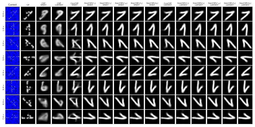
Figure 7: Qualitative examples of the behaviour of the predicted mean of different models when the context set is rotated. We observe that the ConvCNP, even when trained on rotation augmented data, has trouble predicting good shapes when the context set is rotated. By comparison the equivariant models have very consistent predictions under rotation, with the $C_{4}$ and $D_{4}$ models beng exactly equivariant to $90^{\circ}$ rotations, and the $C_{16}$ models being exactly equivariant to $22.5^{\circ}$ rotations

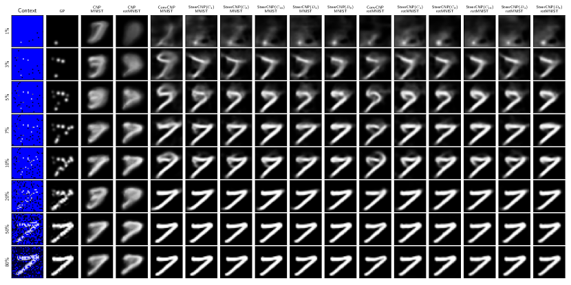
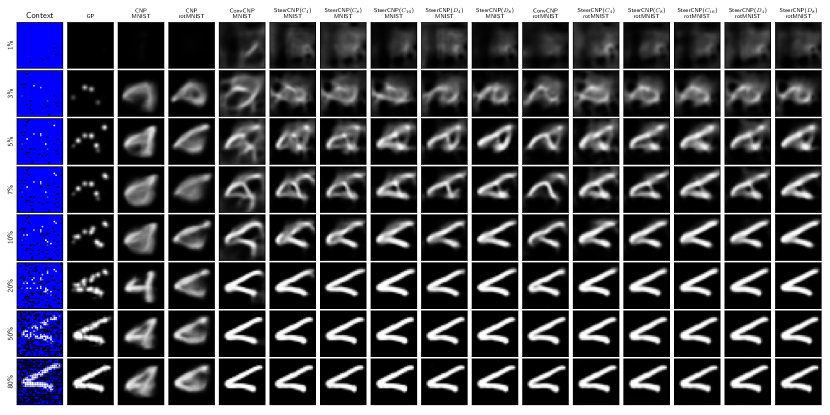
Figure 8: Qualitative examples of the behaviour of the predicted mean of different models when the context set size is changed. Digit not rotated.

Figure 9: Qualitative examples of the behaviour of the predicted mean of different models when the context set size is changed. Digit rotated.

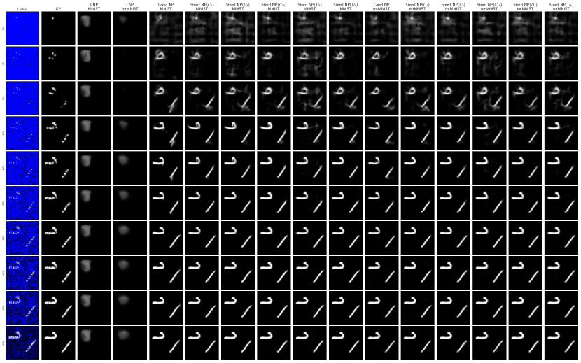
Figure 10: Qualitative examples of the behaviour of models trained on single MNIST digits, tested on multiple digits pasted into a larger canvas. Size of context set varied. We see that further away from the digits there is some noise predictions. These are likely causes by the models never having seen data as far from digits as this, leading to somewhat undefined behaviour. We see that the equivariant models exhibit considerably less of this noisy behaviour.

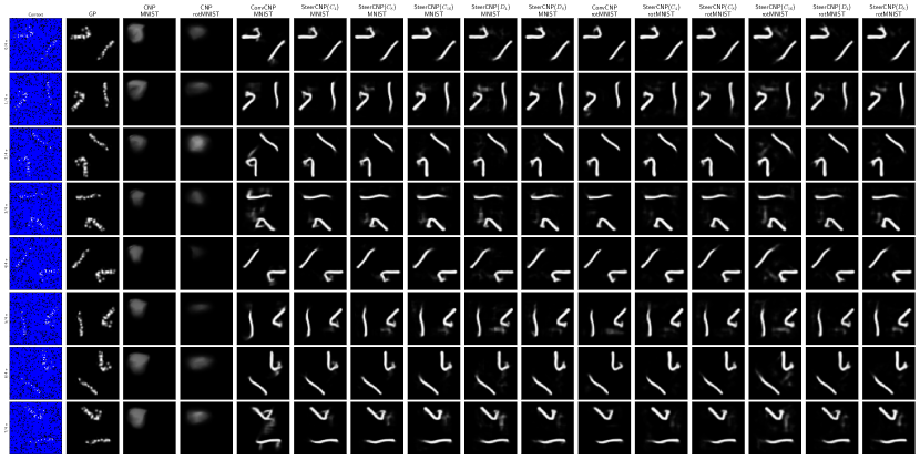
Figure 11: Qualitative examples of the behaviour of models trained on single MNIST digits, tested on multiple digits pasted into a larger canvas. Rotation of the context set is varied. We see that the equivariant models show very little change in behaviour under rotation, whereas the ConvCNP gives reasonably wild predictions under rotation.

References

- Álvarez et al. (2012) Álvarez, M. A., Rosasco, L., and Lawrence, N. D. Kernels for vector-valued functions: A review. Found. Trends Mach. Learn., 4(3):195–266, March 2012. ISSN 1935-8237. doi: 10.1561/2200000036.
- Andrychowicz et al. (2016) Andrychowicz, M., Denil, M., Colmenarejo, S. G., Hoffman, M. W., Pfau, D., Schaul, T., and de Freitas, N. Learning to learn by gradient descent by gradient descent. CoRR, abs/1606.04474, 2016.
- Artin (2011) Artin, M. Algebra. Pearson Prentice Hall, 2011. ISBN 9780132413770.
- Brault et al. (2016) Brault, R., Heinonen, M., and Buc, F. Random Fourier Features For Operator-Valued Kernels. In Asian Conference on Machine Learning, pp. 110–125. PMLR, November 2016. ISSN: 1938-7228.
- Bröcker & Dieck (2003) Bröcker, T. and Dieck, T. Representations of Compact Lie Groups. Graduate Texts in Mathematics. Springer Berlin Heidelberg, 2003. ISBN 9783540136781.
- Bruinsma et al. (2021) Bruinsma, W., Requeima, J., Foong, A. Y. K., Gordon, J., and Turner, R. E. The Gaussian Neural Process. In Third Symposium on Advances in Approximate Bayesian Inference, 2021.
- Cohen & Welling (2016) Cohen, T. and Welling, M. Group equivariant convolutional networks. In Proceedings of The 33rd International Conference on Machine Learning, volume 48 of Proceedings of Machine Learning Research, pp. 2990–2999, New York, New York, USA, 20–22 Jun 2016. PMLR.
- Cohen & Welling (2017) Cohen, T. S. and Welling, M. Steerable CNNs. In 5th International Conference on Learning Representations, ICLR 2017, Toulon, France, April 24-26, 2017, Conference Track Proceedings. OpenReview.net, 2017.
- Cohen et al. (2018) Cohen, T. S., Geiger, M., Köhler, J., and Welling, M. Spherical CNNs. In International Conference on Learning Representations, 2018.
- Cohen et al. (2019) Cohen, T. S., Geiger, M., and Weiler, M. A general theory of equivariant CNNs on homogeneous spaces. In Advances in Neural Information Processing Systems, volume 32, pp. 9145–9156. Curran Associates, Inc., 2019.
- Dieleman et al. (2016) Dieleman, S., Fauw, J. D., and Kavukcuoglu, K. Exploiting cyclic symmetry in convolutional neural networks. In Proceedings of The 33rd International Conference on Machine Learning, volume 48 of Proceedings of Machine Learning Research, pp. 1889–1898, New York, New York, USA, 20–22 Jun 2016. PMLR.
- Esteves et al. (2020) Esteves, C., Makadia, A., and Daniilidis, K. Spin-weighted spherical CNNs. In Advances in Neural Information Processing Systems, 2020.
- Finn et al. (2017) Finn, C., Abbeel, P., and Levine, S. Model-agnostic meta-learning for fast adaptation of deep networks. In Proceedings of the 34th International Conference on Machine Learning, volume 70 of Proceedings of Machine Learning Research, pp. 1126–1135. PMLR, 06–11 Aug 2017.
- Finzi et al. (2020a) Finzi, M., Stanton, S., Izmailov, P., and Wilson, A. G. Generalizing convolutional neural networks for equivariance to Lie groups on arbitrary continuous data. In Proceedings of the 37th International Conference on Machine Learning, volume 119 of Proceedings of Machine Learning Research, pp. 3165–3176. PMLR, 13–18 Jul 2020a.
- Finzi et al. (2020b) Finzi, M., Stanton, S., Izmailov, P., and Wilson, A. G. Generalizing convolutional neural networks for equivariance to lie groups on arbitrary continuous data. In International Conference on Machine Learning, pp. 3165–3176. PMLR, 2020b.
- Foong et al. (2020) Foong, A. Y. K., Bruinsma, W., Gordon, J., Dubois, Y., Requeima, J., and Turner, R. Meta-learning stationary stochastic process prediction with convolutional neural processes. ArXiv, abs/2007.01332, 2020.
- Garnelo et al. (2018a) Garnelo, M., Rosenbaum, D., Maddison, C., Ramalho, T., Saxton, D., Shanahan, M., Teh, Y. W., Rezende, D., and Eslami, S. M. A. Conditional Neural Processes. In Proceedings of the 35th International Conference on Machine Learning, volume 80 of Proceedings of Machine Learning Research, pp. 1704–1713. PMLR, 10–15 Jul 2018a.
- Garnelo et al. (2018b) Garnelo, M., Schwarz, J., Rosenbaum, D., Viola, F., Rezende, D. J., Eslami, S. M. A., and Teh, Y. W. Neural Processes. CoRR, abs/1807.01622, 2018b.
- Goovaerts et al. (1997) Goovaerts, P. et al. Geostatistics for natural resources evaluation. Oxford University Press on Demand, 1997.
- Gordon et al. (2020) Gordon, J., Bruinsma, W. P., Foong, A. Y. K., Requeima, J., Dubois, Y., and Turner, R. E. Convolutional Conditional Neural Processes. In International Conference on Learning Representations, 2020.
- Harris et al. (2020) Harris, C. R., Millman, K. J., van der Walt, S. J., Gommers, R., Virtanen, P., Cournapeau, D., Wieser, E., Taylor, J., Berg, S., Smith, N. J., et al. Array programming with numpy. Nature, 585(7825):357–362, 2020.
- Hoogeboom et al. (2018) Hoogeboom, E., Peters, J. W., Cohen, T. S., and Welling, M. Hexaconv. In International Conference on Learning Representations, 2018.
- Hunter (2007) Hunter, J. D. Matplotlib: A 2d graphics environment. Computing in science & engineering, 9(3):90–95, 2007.
- Hutchinson et al. (2020) Hutchinson, M., Lan, C. L., Zaidi, S., Dupont, E., Teh, Y. W., and Kim, H. Lietransformer: Equivariant self-attention for lie groups. arXiv preprint arXiv:2012.10885, 2020.
- Jones et al. (2001) Jones, E., Oliphant, T., Peterson, P., et al. Scipy: Open source scientific tools for python. 2001.
- Kawano et al. (2021) Kawano, M., Kumagai, W., Sannai, A., Iwasawa, Y., and Matsuo, Y. Group Equivariant Conditional Neural Processes. In International Conference on Learning Representations, 2021.
- Kim et al. (2019) Kim, H., Mnih, A., Schwarz, J., Garnelo, M., Eslami, A., Rosenbaum, D., Vinyals, O., and Teh, Y. W. Attentive Neural Processes. In International Conference on Learning Representations, 2019.
- Kingma & Ba (2015) Kingma, P. and Ba, J. Adam: A method for stochastic optimization, arxiv (2014). In 3rd International Conference on Learning Representations, 2015.
- Kondor & Trivedi (2018) Kondor, R. and Trivedi, S. On the generalization of equivariance and convolution in neural networks to the action of compact groups. In Proceedings of the 35th International Conference on Machine Learning, volume 80 of Proceedings of Machine Learning Research, pp. 2747–2755. PMLR, 10–15 Jul 2018.
- Landau (2013) Landau, L. D. The classical theory of fields, volume 2. Elsevier, 2013.
- LeCun et al. (1990) LeCun, Y., Boser, B. E., Denker, J. S., Henderson, D., Howard, R. E., Hubbard, W. E., and Jackel, L. D. Handwritten digit recognition with a back-propagation network. In Advances in Neural Information Processing Systems 2, pp. 396–404. Morgan-Kaufmann, 1990.
- LeCun et al. (2010) LeCun, Y., Cortes, C., and Burges, C. MNIST handwritten digit database. ATT Labs [Online]. Available: http://yann.lecun.com/exdb/mnist, 2, 2010.
- Macêdo & Castro (2010) Macêdo, I. and Castro, R. Learning divergence-free and curl-free vector fields with matrix-valued kernels. IMPA, 2010.
- Oliphant (2006) Oliphant, T. E. A guide to NumPy, volume 1. Trelgol Publishing USA, 2006.
- Oliphant (2007) Oliphant, T. E. Python for scientific computing. Computing in Science & Engineering, 9(3):10–20, 2007.
- Paszke et al. (2017a) Paszke, A., Gross, S., Chintala, S., Chanan, G., Yang, E., DeVito, Z., Lin, Z., Desmaison, A., Antiga, L., and Lerer, A. Automatic differentiation in pytorch. 2017a.
- Paszke et al. (2017b) Paszke, A., Gross, S., Chintala, S., Chanan, G., Yang, E., DeVito, Z., Lin, Z., Desmaison, A., Antiga, L., and Lerer, A. Automatic differentiation in pytorch. 2017b.
- Rasmussen & Williams (2005) Rasmussen, C. E. and Williams, C. K. I. Gaussian Processes for Machine Learning (Adaptive Computation and Machine Learning). The MIT Press, 2005. ISBN 026218253X.
- Reisert & Burkhardt (2007) Reisert, M. and Burkhardt, H. Learning equivariant functions with matrix valued kernels. Journal of Machine Learning Research, 8:385–408, 03 2007.
- Satorras et al. (2021) Satorras, V. G., Hoogeboom, E., and Welling, M. E (n) equivariant graph neural networks. arXiv preprint arXiv:2102.09844, 2021.
- Serre (1977) Serre, J. Linear Representations of Finite Groups. Collection Méthodes. Mathématiques. Springer-Verlag, 1977. ISBN 9783540901907.
- Van Rossum & Drake Jr (1995) Van Rossum, G. and Drake Jr, F. L. Python reference manual. Centrum voor Wiskunde en Informatica Amsterdam, 1995.
- Walt et al. (2011) Walt, S. v. d., Colbert, S. C., and Varoquaux, G. The numpy array: a structure for efficient numerical computation. Computing in science & engineering, 13(2):22–30, 2011.
- Wang et al. (2020) Wang, R., Walters, R., and Yu, R. Incorporating symmetry into deep dynamics models for improved generalization. arXiv preprint arXiv:2002.03061, 2020.
- Weiler & Cesa (2019) Weiler, M. and Cesa, G. General E(2)-equivariant steerable CNNs. In Advances in Neural Information Processing Systems, pp. 14334–14345, 2019.
- Weiler et al. (2018) Weiler, M., Geiger, M., Welling, M., Boomsma, W., and Cohen, T. S. 3d Steerable CNNs: Learning rotationally equivariant features in volumetric data. In Advances in Neural Information Processing Systems, volume 31, pp. 10381–10392. Curran Associates, Inc., 2018.
- Worrall & Brostow (2018) Worrall, D. E. and Brostow, G. J. Cubenet: Equivariance to 3d rotation and translation. In Computer Vision - ECCV 2018 - 15th European Conference, Munich, Germany, September 8-14, 2018, Proceedings, Part V, pp. 585–602, 2018. doi: 10.1007/978-3-030-01228-1“˙35.
- Worrall et al. (2016) Worrall, D. E., Garbin, S. J., Turmukhambetov, D., and Brostow, G. J. Harmonic networks: Deep translation and rotation equivariance. CoRR, abs/1612.04642, 2016.
- Øksendal (2000) Øksendal, B. Stochastic Differential Equations: An Introduction with Applications, volume 82. 01 2000. doi: 10.1007/978-3-662-03185-8.