INR-TH-2020-044 Examining axion-like particles with superconducting radio-frequency cavity

Abstract

We address production of massive axion-like particles by two electromagnetic modes inside a superconducting radio-frequency (SRF) cylindrical cavity. We discuss in detail the choice of pump modes and cavity design. We numerically compute time-averaged energy density of produced axion field for various cavity modes and wide range of axion masses. This allows us to estimate optimal conditions for axion production within a cavity. In addition, we consider photon regeneration process initiated by produced axion field in a screened radio-frequency cavity and derive constraints in parameter space $(g_{a\gamma\gamma},\ m_{a})$ for different choice of pump modes.

1 Introduction

Axion-like particles (ALPs) are hypothetical pseudoscalar particles appearing in several extensions of the Standard Model [1]. Original axions were introduced in order to resolve the strong CP-problem in QCD [2, 3]. Later, it was argued that ALPs can appear in a low-energy phenomenological description of string theory [4, 5].

The efforts toward the searches for ALPs include such types of experiments as: helioscopes [6], haloscopes [7, 8, 9], light-shining-through-wall (LSW) experiments [10, 11], space-based gamma-ray telescopes [12], accelerator-based experiments [13, 14, 15, 16], neutrino experiments [17] and reactor experiments [18].

In addition, astrophysics and cosmology observations imply that ALPs are well motivated candidates for dark matter content [19, 20, 21]. Moreover, several exotic scenarios of DM can be associated with ALPs [22, 23]. A properties of axion dark matter are sensitive to the self-interaction parameters. In particular, the relevant dark matter can be clumped into miniclusters [24, 25], or form other inhomogeneous structures [26, 27, 28]. Axion field can also form exotic compact objects (bose stars [29, 30]) providing a possible explanation for fast radio bursts [31, 32].

More generally, the axion field $a$ with mass $m_{a}$ and dimensionful coupling to photons $g_{a\gamma\gamma}$ is described by the Lagrangian

$$\mathcal{L}=-\frac{1}{4}F_{\mu\nu}F^{\mu\nu}+\frac{1}{2}(\partial_{\mu}a)^{2}-\frac{1}{2}{m_{a}}^{2}a^{2}+\frac{g_{a\gamma\gamma}}{4}\,a\,F_{\mu\nu}\tilde{F}^{\mu\nu}\;,$$ (1)

where $F_{\mu\nu}$ is the electromagnetic tensor and $\tilde{F}^{\mu\nu}=\epsilon^{\mu\nu\rho\sigma}F_{\rho\sigma}/2$ is its dual. The Lagrangian (1) yields the following equations for axion and electromagnetic fields,

$$(\partial_{\mu}\partial^{\mu}+{m_{a}}^{2})\,a=\frac{g_{a\gamma\gamma}}{4}F_{\mu\nu}\tilde{F}^{\mu\nu}\,,$$ (2)

$$\partial_{\mu}F^{\mu\nu}=g_{a\gamma\gamma}\,\tilde{F}^{\mu\nu}\partial_{\mu}a.$$ (3)

If the electromagnetic invariant $F_{\mu\nu}\tilde{F}^{\mu\nu}=-4(\vec{E}\cdot\vec{B})$ is non-vanishing then Eq. (2) implies that axion field can be produced. This may be realized in laboratory by combination of two strong electromagnetic (EM) waves or by a single EM wave in a strong magnetic field. Strong enough EM field with high level of coherence can be produced within optical range by lasers or within radio-frequency range inside SRF cavities.

The axion field once being produced may interact with the EM field in a non-linear way according to Eq. (3). So that the axion-induced EM field may be detected within the same production cavity [33] or within an additional detection cavity [34, 35, 36]. In the latter case both cavities should be screened in order to suppress the external EM field penetration. This setup illustrates so-called LSW type of laboratory experiments for axion searches. For instance, both production and detection cavities are filled with the strong magnetic field in order to initiate effective axion-photon conversion.

This setup was proposed and realized for both optical [37] and RF ranges [34]. Both optical LSW experiment ALPS [38] and RF experiment CROWS [39] gives the same order of magnitude constraints (for details see Ref. [1]) in the plane $(g_{a\gamma\gamma},m_{a})$. In particularly, for small axion masses one has $g_{a\gamma\gamma}\lesssim 10^{-7}\,\mbox{GeV}^{-1}$, which is still the best pure laboratory constraint. Although significantly better constraints (up to $g_{a\gamma\gamma}\lesssim 10^{-10}\,\mbox{GeV}^{-1}$) come from null results of dark matter searches or solar axion detection (see, e. g. Ref.  [6]), these constraints are sensitive to the model of axion production. On the other hand, the production of ALPs in laboratory experiments is straightforward. However, both cosmic and laboratory methods for ALPs searches complement each others.

The classical LSW setup requires external magnetic field in both production and detection cavities. However, the quality factor of cavities is constrained at level $Q\lesssim 10^{5}$ that implies the limitation on the amplitude of cavity modes. Therefore, sensitivity of ALPs detection decreases. The much bigger quality factor $Q\sim 10^{12}$ can be achieved with superconducting radiofrequency (SRF) cavities, but the price to be payed is that one can not apply strong magnetic field inside the cavity due to degradation of surepconducting state. The maximal amplitudes for SRF cavity modes are constrained by the overall magnetic field near the cavity walls. In particular, for superconducting niobium [41] the critical magnetic field is $\sim 0.2$ T. Given that constraint, the authors of Ref. [35] suggested the LSW setup involving cylindrical SRF production cavity and toroidal SRF detector. Moreover, it was pointed out that sensitivity depends essentially on the geometrical formfactor for emitter and converter cavities.

In our paper we address this issue in detail. In particular, we discuss spatial distributions of the produced axion field in cylindrical SRF cavities. We also estimate detection sensitivity of the cylindrical RF cavity ($Q\sim 10^{5}$) filled with the strong magnetic field, so that it can reach $10$ T. Recently, a similar setup was suggested in Ref. [36], particularly, authors discuss the LSW facility to probe ALPs with two screened cylindrical SRF cavities which are served as emitter and receiver of axion field respectively. The setup allows to achieve relatively large quality factors $Q\sim 10^{12}$, however, the peak EM field in the cavities is constrained by $\lesssim 0.2$ T. We show that sensitivity to probe ALPs in our LSW setup $g_{a\gamma\gamma}\lesssim\mathcal{O}(1)\times 10^{-11}\,\mbox{GeV}^{-1}$ is comparable to that performed in Ref. [36].

In Ref. [33] authors suggested the setup to probe ALPs inside a single SRF cavity filled with different modes. Axion-like particles realize a non-linear coupling between those modes. Absence of the magnetic field allows to achieve the quality factor $Q\sim 10^{12}$. However, sensitivity is leveraged by relatively small magnitude of magnetic field $\lesssim 0.2$ T allowed in SRF. We show that our LSW setup is also sensitive to probe ALPs for the region of parameter space, which is close to one discussed in Ref. [33].

This paper is organized as follows. In Sec. 2 we consider ALPs production using Green function approach. In Sec. 3 we present results of numerical calculation for time-averaged energy density of axion field initiated by different pairs of cylindrical cavity eigenmodes. In Sec. 4 we consider ALPs detection in the RF cavity with the strong magnetic field. We also estimate constraints in the parameter space $(g_{a\gamma\gamma},m_{a})$. In Sec. 5 we discuss obtained results. Appendices contain technical details.

2 ALP production in superconducting cavity

In this section we consider production of the axion field by electromagnetic radio-frequency modes pumped into a superconducting cavity. The generated axion field is described by a solution of Eq. (2) respecting causality. In particular, it is given by

$$a(\vec{x},t)=\int\limits_{-\infty}^{\infty}dt^{\prime}\int\limits_{V_{\mathrm{cav}}}d^{3}x^{\prime}\,G_{\mathrm{ret}}(\vec{x}-\vec{x}^{\prime},t-t^{\prime})\;\times\;\left[-g_{a\gamma\gamma}\,\left(\vec{E}(\vec{x}^{\prime},t^{\prime})\cdot\vec{B}(\vec{x}^{\prime},t^{\prime})\right)\right]\;,$$ (4)

where $G_{\mathrm{ret}}(\vec{x}-\vec{x}^{\prime},t-t^{\prime})$ is the retarded Green function, $\vec{E}(\vec{x}^{\prime},t^{\prime})$ and $\vec{B}(\vec{x}^{\prime},t^{\prime})$ are the electric and magnetic fields respectively inside the cavity of volume $V_{\mathrm{cav}}$. Since for a single cavity mode the electric field is orthogonal to the magnetic one, at least two cavity modes are necessary for ALPs productions. Therefore, one reads $\vec{E}(\vec{x},t)=\vec{E}_{1}(\vec{x},t)+\vec{E}_{2}(\vec{x},t)$ and $\vec{B}(\vec{x},t)=\vec{B}_{1}(\vec{x},t)+\vec{B}_{2}(\vec{x},t)$ for the electric and magnetic fields correspondingly, where the subscripts refer to the cavity modes at given frequencies $\omega_{1,\,2}$.

The time dependence for each mode decouples as follows

$$\vec{E}_{i}(\vec{x},t)=\sqrt{2}\Re\mathrm{e}\left[\vec{{\cal E}}_{i}(\vec{x},\omega_{i})e^{-i\omega_{i}t}\right]\;,\qquad\qquad\vec{B}_{i}(\vec{x},t)=\sqrt{2}\Re\mathrm{e}\left[\vec{{\cal B}}_{i}(\vec{x},\omega_{i})e^{-i\omega_{i}t}\right]\;,$$

where $\vec{{\cal E}}_{i}(\vec{x},\omega_{i})$ are cavity eigenmodes without proper normalization to take into account its arbitrary amplitudes. The electromagnetic invariant $(\vec{E}\cdot\vec{B})$ for two modes can be represented as

$$\left(\vec{E}(\vec{x},t)\cdot\vec{B}(\vec{x},t)\right)=\Re\mathrm{e}\left[F_{+}(\vec{x})\cdot\mathrm{e}^{-i\omega_{+}t}+F_{-}(\vec{x})\cdot\mathrm{e}^{-i\omega_{-}t}\right]\;,$$ (5)

where we defined $\omega_{\pm}=\omega_{2}\pm\omega_{1}$ and

$$F_{+}(\vec{x})\equiv\vec{{\cal E}}_{1}(\vec{x})\cdot\vec{{\cal B}}_{2}(\vec{x})+\vec{{\cal E}}_{2}(\vec{x})\cdot\vec{{\cal B}}_{1}(\vec{x})\;,\qquad F_{-}(\vec{x})\equiv\vec{{\cal E}}_{1}^{*}(\vec{x})\cdot\vec{{\cal B}}_{2}(\vec{x})+\vec{{\cal E}}_{2}(\vec{x})\cdot\vec{{\cal B}}_{1}^{*}(\vec{x})\;.$$

Note that we consider cavity modes where the electric and magnetic fields are orthogonal, so that $(\vec{{\cal E}}_{i}(\vec{x})\cdot\vec{{\cal B}}_{i}(\vec{x}))=0$ everywhere inside the cavity.

Since Eq. (2) is linear with respect to $a$, one has independent propagation for each frequency component in Eq. (5). The produced axion field is then given by $a(\vec{x},t)=a_{+}(\vec{x},t)+a_{-}(\vec{x},t)$, where $a_{\pm}(\vec{x},t)$ are independent components for $\omega_{\pm}$. One can easily integrate out $t^{\prime}$ in Eq. (4) for two cases depending on axion mass (see e. g. Appendix A),

$$m_{a}<\omega_{\pm}:\qquad\qquad a_{\pm}(\vec{x},t)=-g_{a\gamma\gamma}\;\Re\mathrm{e}\,\int\limits_{V_{\mathrm{cav}}}d^{3}x^{\prime}\,\frac{F_{\pm}(\vec{x}^{\prime})}{4\pi|\vec{x}-\vec{x}^{\prime}|}\mathrm{e}^{-i\omega_{\pm}t+i|\vec{x}-\vec{x}^{\prime}|k_{\pm}}\;.$$ (6)

$$m_{a}>\omega_{\pm}:\qquad\qquad a_{\pm}(\vec{x},t)=-g_{a\gamma\gamma}\;\Re\mathrm{e}\,\int\limits_{V_{\mathrm{cav}}}d^{3}x^{\prime}\,\frac{F_{\pm}(\vec{x}^{\prime})}{4\pi|\vec{x}-\vec{x}^{\prime}|}\mathrm{e}^{-i\omega_{\pm}t-|\vec{x}-\vec{x}^{\prime}|\kappa_{\pm}}\;,$$ (7)

where $k_{\pm}\equiv\sqrt{\omega_{\pm}^{2}-m_{a}^{2}}$. For the case $m_{a}>\omega_{\pm}$ Eq. (7) is obtained formally by a replacement of $ik_{\pm}$ in Eq. (6) by $\kappa_{\pm}=\sqrt{m_{a}^{2}-\omega_{\pm}^{2}}$, so that the axion field amplitude decreases exponentially far from the cavity volume. We note that the functions $F_{\pm}(\vec{x}^{\prime})$ are generally complex what may give an additional phase of the integrand in Eqs. (6)-(7).

Since the axion field amplitude harmonically oscillates the time-averaged $a_{\pm}(\vec{x},t)$ goes to zero. Instead, we consider the following time-averaging,

$$\braket{a^{2}}=\frac{1}{T}\int\limits^{T}_{0}dt\,\,a^{2}(t)=\frac{1}{T}\int\limits^{T}_{0}dt\,\,(a_{+}(t)+a_{-}(t))^{2}=\braket{a_{+}^{2}}+\braket{a_{-}^{2}}\;,$$ (8)

where the mixed term $\braket{a_{+}a_{-}}$ vanishes because $a_{+}a_{-}$ is a sum of products of two harmonic functions with different frequencies and averaging over time period yields zero.

For two non-zero terms in Eq. (8) we obtain

$$m_{a}<\omega_{\pm}:\qquad\qquad \braket{a^{2}_{\pm}}=\frac{1}{2}\left(\left(A_{\pm}^{C}\right)^{2}+\left(A_{\pm}^{S}\right)^{2}\right)\;,$$ (9)

$$m_{a}>\omega_{\pm}:\qquad\qquad \braket{a^{2}_{\pm}}=\frac{1}{2}B_{\pm}^{2}\;,$$ (10)

where

$$A^{C(S)}_{\pm}=g_{a\gamma\gamma}\,\int\limits_{V_{\mathrm{cav}}}d^{3}x^{\prime}\,\frac{\left|F_{\pm}(\vec{x}^{\prime})\right|}{4\pi|\vec{x}-\vec{x}^{\prime}|}\left\{\begin{array}[]{c}\cos\left(k_{\pm}|\vec{x}-\vec{x}^{\prime}|\right)\\ \sin\left(k_{\pm}|\vec{x}-\vec{x}^{\prime}|\right)\end{array}\right\}\;,$$ (11)

$$B_{\pm}=g_{a\gamma\gamma}\,\int\limits_{V_{\mathrm{cav}}}d^{3}x^{\prime}\,\frac{\left|F_{\pm}(\vec{x}^{\prime})\right|}{4\pi|\vec{x}-\vec{x}^{\prime}|}\mathrm{e}^{-\kappa_{\pm}|\vec{x}-\vec{x}^{\prime}|}\;.$$ (12)

For a specific resonant case $m_{a}=\omega_{\pm}$ one has $k_{\pm}=\kappa_{\pm}=0$, so that

$$\left.A^{C}_{\pm}\right|_{\mathrm{res}}=\left.B_{\pm}\right|_{\mathrm{res}}=g_{a\gamma\gamma}\,\int\limits_{V_{\mathrm{cav}}}d^{3}x^{\prime}\,\frac{\left|F_{\pm}(\vec{x}^{\prime})\right|}{4\pi|\vec{x}-\vec{x}^{\prime}|}\;,\qquad\left.A^{S}_{\pm}\right|_{\mathrm{res}}=0\;.$$ (13)

Next, far away from the cavity the integral $\int d^{3}x^{\prime}\left|F_{\pm}(\vec{x}^{\prime})\right|/|\vec{x}-\vec{x}^{\prime}|$ is suppressed for two transversal magnetic modes in the cavity (TM+TM), since their overlap factor $\int d^{3}x^{\prime}\left|F_{\pm}(\vec{x}^{\prime})\right|$ is negligible. In that case the resonant production of ALPs in SRF cavity is ineffective. In addition we note that for two transversal electric modes (TE+TE) or transversal magnetic and electric modes (TM+TE) this overlap integral can be significant. Therefore the resonant production of ALPs for these combinations of modes is more efficient.

To conclude this section let us list the formulae for the energy density of the generated axion field,

$$\rho^{E}_{\pm}=\frac{1}{2}\dot{a}^{2}+\frac{1}{2}(\partial_{i}a)^{2}+\frac{m_{a}^{2}}{2}a^{2}\;.$$ (14)

In particular, for various masses $m_{a}$ of the axion field the time-averaged value $\langle\rho^{E}_{\pm}\rangle$ can be written as follows,

$$m_{a}<\omega_{\pm}: \qquad\braket{\rho^{E}_{\pm}}=\frac{1}{4}\left(\left[m_{a}^{2}+\omega^{2}_{\pm}\right]((A_{\pm}^{S})^{2}+(A_{\pm}^{C})^{2})+(\partial_{i}A_{\pm}^{S})^{2}+(\partial_{i}A_{\pm}^{C})^{2}\right)\;,$$ (15)

$$m_{a}>\omega_{\pm}: \qquad\braket{\rho^{E}_{\pm}}=\frac{1}{4}\left(\left[m_{a}^{2}+\omega^{2}_{\pm}\right]B_{\pm}^{2}+(\partial_{i}B_{\pm})^{2}\right)\;,$$ (16)

where $A_{\pm}^{C(S)}$ and $B_{\pm}$ are given by Eqs. (11)-(12). In Sec. 3 we discuss spatial distributions for the given quantities and study its properties for the resonant case $m_{a}\simeq\omega_{+}$.

3 Numerical results for ALP production in cylindrical cavity

In this Section we consider axion production in cylindrical cavity. We use TE$npq$/TM$npq$ notation to classify EM cavity modes [42]. Given a height $L$ and a radius $R$ of the cavity one has the following dispersion relations for TM and TE modes respectively,

$$\omega^{TM}_{npq}=\sqrt{\left(\frac{x_{np}}{R}\right)^{2}+\left(\frac{q\pi}{L}\right)^{2}},\qquad\qquad\omega^{TE}_{npq}=\sqrt{\left(\frac{x^{\prime}_{np}}{R}\right)^{2}+\left(\frac{q\pi}{L}\right)^{2}}\;,$$ (17)

where $x_{np}$ and $x^{\prime}_{np}$ are p-th roots of the n-th order Bessel function $J_{n}(x)$ and its derivative $J^{\prime}_{n}(x)$ correspondingly. Integers $n,\,p,\,q$ enumerate the full set of modes and refer to the “winding” numbers in $\phi,\,\rho,\,z$ directions respectively. The explicit expressions for the given set of modes are presented in Appendix B.

One has to consider the following combinations of pump cavity modes: (i) TM+TM, (ii) TE+TE, (iii) TE+TM. It is straightforward to show using expressions from Appendix B that for (i) and (ii) cases the functions $F_{+}$ and $F_{-}$ are purely imaginary and for the case (iii) $F_{+}$ and $F_{-}$ are purely real. Since ${\cal E}^{TE}_{z}={\cal B}^{TM}_{z}=0$ one has

$$(TE+TM):\qquad\left|F_{\pm}\right|=\left|{\cal E}_{z}^{TM}{\cal B}_{z}^{TE}+{\cal E}_{\rho}^{TM}{\cal B}_{\rho}^{TE}+{\cal E}_{\phi}^{TM}{\cal B}_{\phi}^{TE}\pm\left({\cal E}_{\rho}^{TE}{\cal B}_{\rho}^{TM}+{\cal E}_{\phi}^{TE}{\cal B}_{\phi}^{TM}\right)\right|\;,$$ (18)

$$(TE+TE\text{ or }TM+TM):\qquad\left|F_{\pm}\right|=\left|{\cal E}_{\rho}^{1}{\cal B}_{\rho}^{2}+{\cal E}_{\phi}^{1}{\cal B}_{\phi}^{2}\pm\left({\cal E}_{\rho}^{2}{\cal B}_{\rho}^{1}+{\cal E}_{\phi}^{2}{\cal B}_{\phi}^{1}\right)\right|\;.$$ (19)

Functions $F_{\pm}$ vanish for the cases (i) and (ii) as soon as its “winding” numbers $n_{1}=n_{2}=0$. On the other hand, two modes with zero $n$ give non-vanishing terms for the case (iii).

We performed numerical calculations [43] of the time-averaged axion energy density $\braket{\rho^{E}_{\pm}}$ generated by two TE/TM modes in the cylindrical cavity with various dimensions $R$ and $L$. We also assumed $g_{a\gamma\gamma}=10^{-10}\,\mbox{GeV}^{-1}$ as a benchmark for ALPs coupling. One also has to fix the amplitudes ${\cal E}_{0}$ (${\cal B}_{0}$), which appears as a normalization constants in the expressions for mode components ${\cal E}_{z}^{TM}$ (${\cal B}_{z}^{TE}$) of Appendix B. Its maximum value is limited by a requirement that the magnetic field on the superconducting cavity walls should not exceed the critical value $\sim 0.1$ T. We note that the components ${\cal E}^{TM}_{\rho}$ (${\cal B}^{TE}_{\rho}$) and ${\cal E}^{TM}_{\phi}$ (${\cal B}^{TE}_{\phi}$) can be larger than ${\cal E}_{0}$ (${\cal B}$) for a “pancake-like” design of the cylindrical cavity with $R\gg L$. Therefore, in numerical calculations we require typical values $|\vec{{\cal E}}|$, $|\vec{{\cal B}}|\lesssim 0.1$ T for both TM and TE modes.

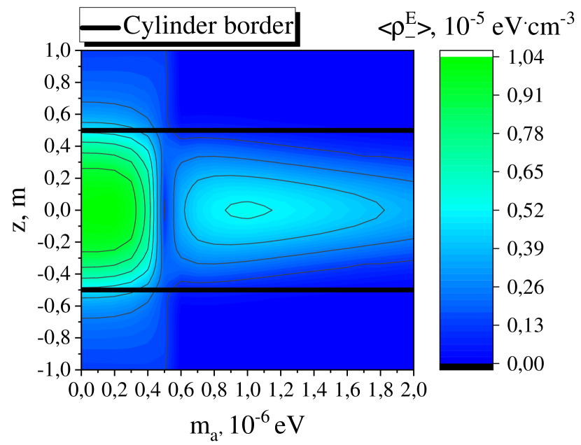
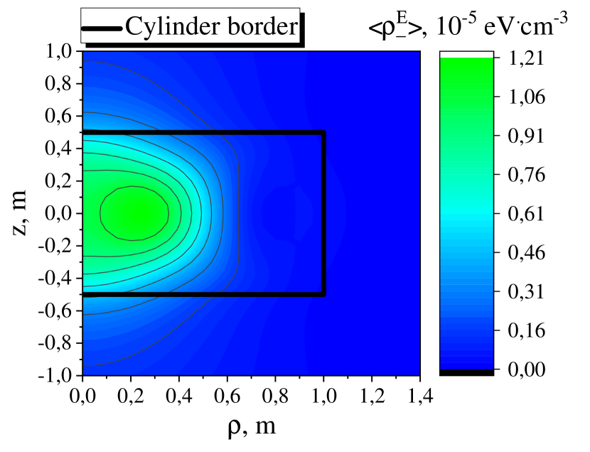
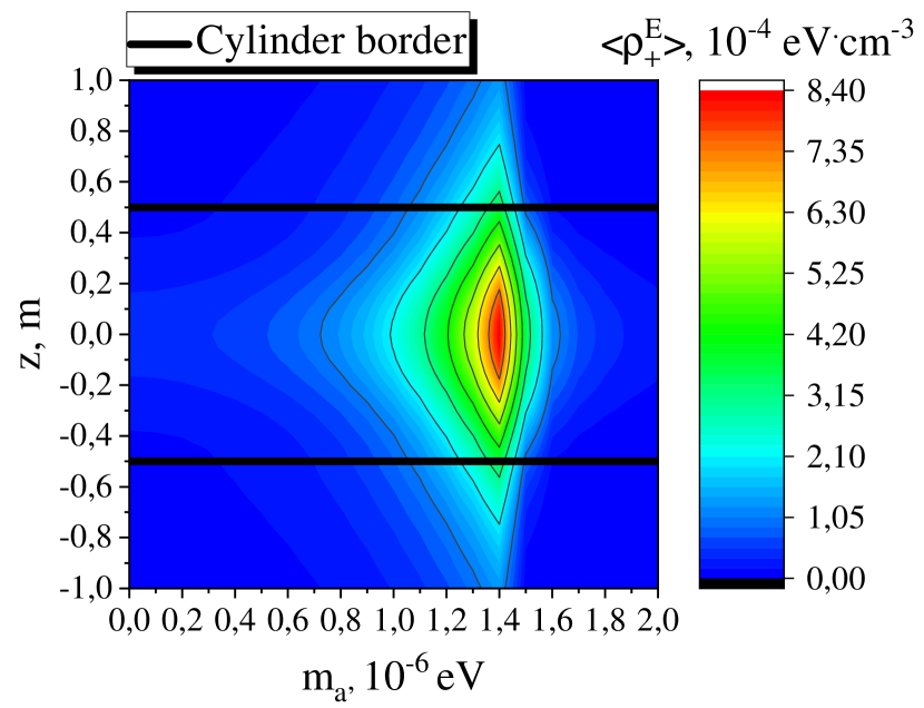
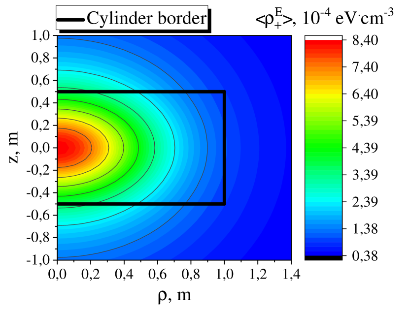
Figure 1: Results of numerical calculations for TM010+TE011 pump modes. Top: Contour plots for the time-averaged energy densities $\braket{\rho^{E}_{-}}$ and $\braket{\rho^{E}_{+}}$ evaluated on the cylinder axis as function of axion mass $m_{a}$ and distance $z$ from center of cavity with TM010+TE011 pump modes. Cavity dimensions: $L=1$ m, $R=1$ m. Left panel: $\omega_{-}=5.1\cdot 10^{-7}$ eV. Right panel: $\omega_{+}=14.7\cdot 10^{-7}$ eV. Bottom: Spatial distribution of the time-averaged energy density $\braket{\rho^{E}_{-}}$ and $\braket{\rho^{E}_{+}}$ on the cavity section along its axis $(\rho,\,z)$ with TM010+TE011 pump modes. Cavity dimensions: $L=1$ m, $R=1$ m. Left panel: $m_{a}=0$, $\omega_{-}=5.1\cdot 10^{-7}$ eV. Right panel: $m_{a}=\omega_{+}=14.7\cdot 10^{-7}$ eV.

Let us consider the production cavity with dimensions $R=L=1$ m and the simplest combination of pump modes TM010+TE011. The evaluated axion energy density for each frequency component $a_{\pm}$ is presented in Fig. 1. Plots at the top in Fig. 1 show the time-averaged energy density on the cylinder axis ($\rho=0$) as function of both distance from the cavity center $z$ and axion mass $m_{a}$. Top-right panel in Fig. 1 shows the resonance in $\langle\rho^{E}_{+}(m_{a}\simeq\omega_{+})\rangle$ in the center of cavity. On the other hand, on the top-left panel in Fig. 1 one can see a significant suppression of $\langle\rho^{E}_{-}\rangle$ in the center of cavity and relatively larger amplitude at $m_{a}=0$. That suppression can be explained as follows. One can see that $F_{-}$ in Eq. (18) is a difference between two positive terms of the same order of magnitude, which compensate each other. However $F_{+}$ is a sum of the relevant terms. Therefore the energy density associated with $\omega_{+}$ is almost two orders of magnitude larger than that for $\omega_{-}$.

The spatial distribution of energy density as function of radius $\rho$ and height $z$ is shown at the bottom in Fig. 1. These plots respect an axial symmetry since the chosen cavity modes do not depend on $\phi$. Distributions for $\omega_{+}$ and $\omega_{-}$ components of axion field were calculated for the cases $m_{a}=\omega_{+}$ and $m_{a}=0$ respectively. For both cases the axion energy density is localized close to center of the production cavity and decreases outside the cavity. In particular, the energy density $\langle\rho_{+}^{E}\rangle$ near the cavity ends at $z=0.5$ m drops by factor 2 with respect to a resonant value at $z=0$ m.

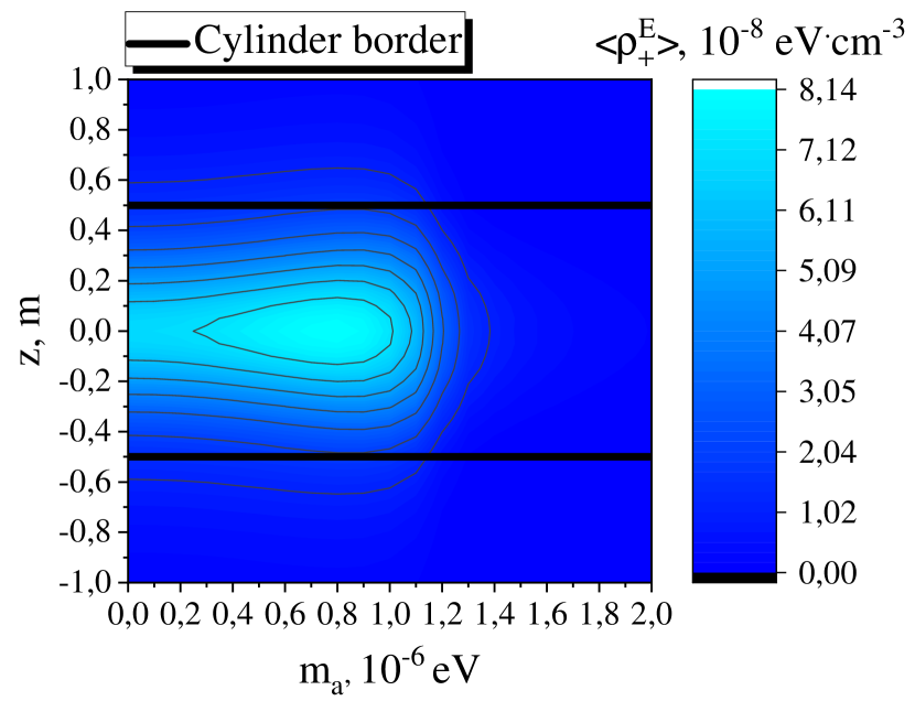
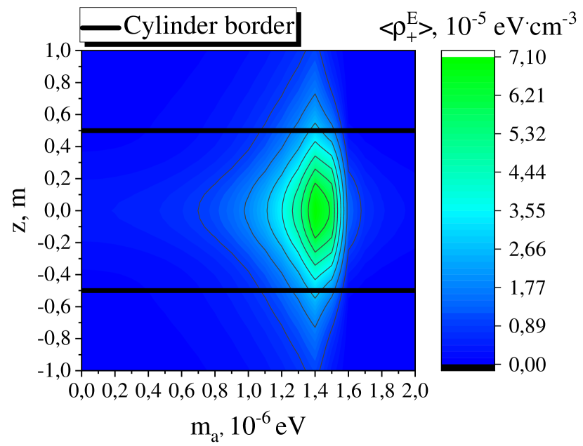
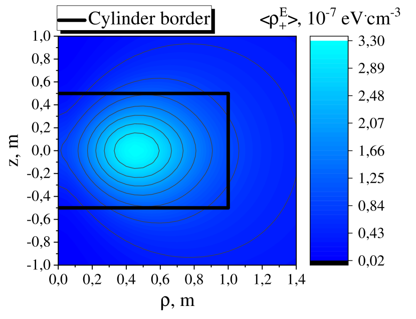
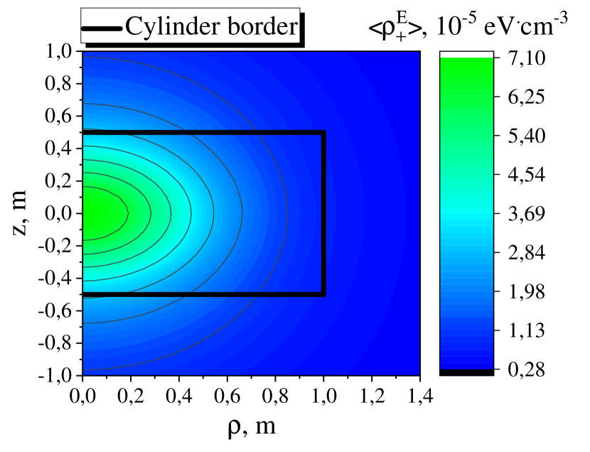
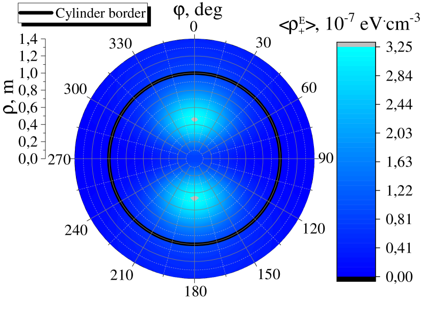
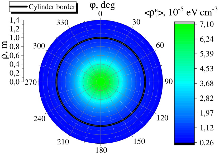
Figure 5: Contour plot for the time-averaged energy density $\braket{\rho^{E}_{+}}$ evaluated on the cylinder axis as function of axion mass $m_{a}$ and the distance $z$ from center of cavity (left panels) and spatial distribution of $\braket{\rho^{E}_{+}}$ on the cavity section along its axis $(\rho,\,z)$ (middle panels) and $(\rho,\,\varphi)$ (right panels) with TM010+TE111 $\omega_{+}=12.1\cdot 10^{-7}$eV (top), TM110+TE111 $\omega_{+}=14.9\cdot 10^{-7}$ eV (bottom) pump modes. Cavity dimensions: $L=1$ m, $R=1$ m.

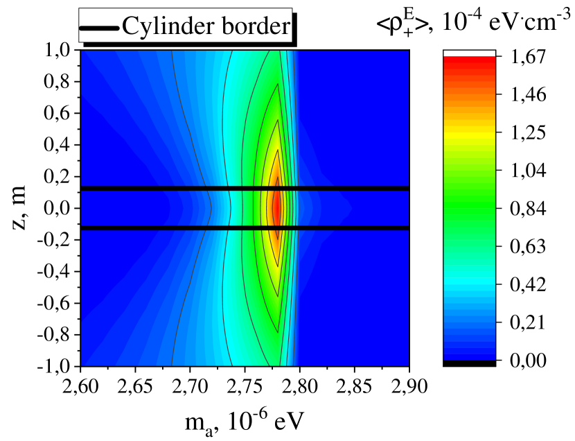
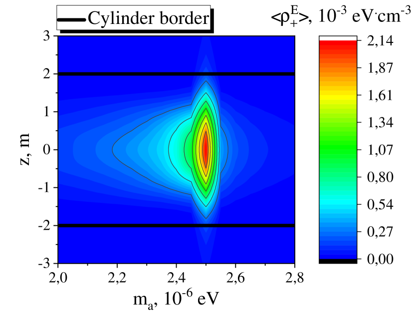
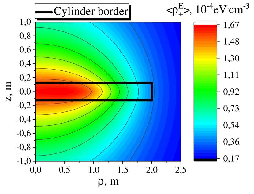
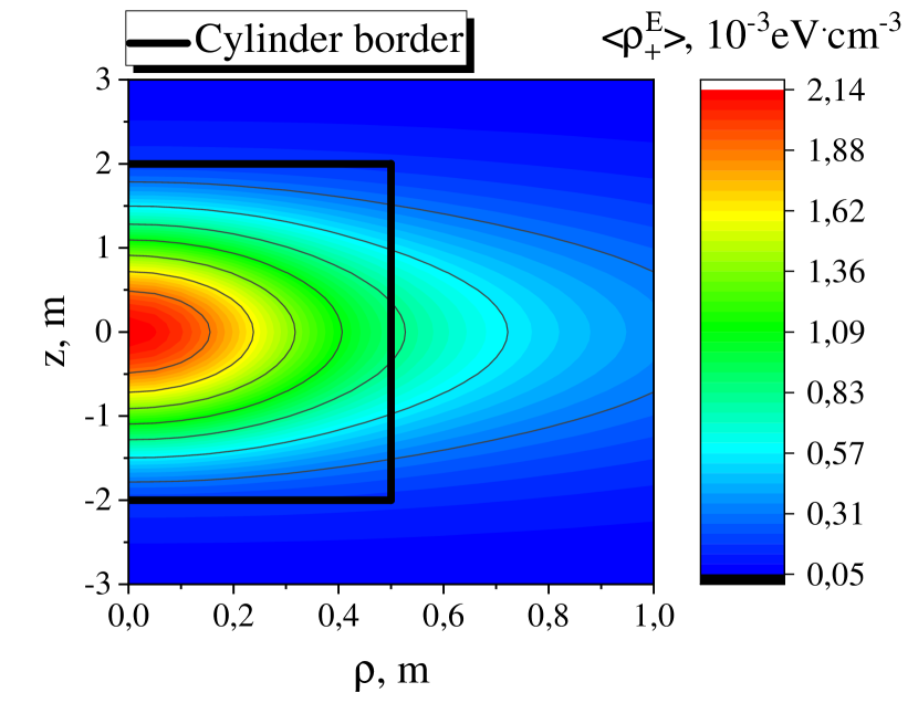
Figure 6: Contour plot for the time-averaged energy density $\braket{\rho^{E}_{+}}$ evaluated on the cylinder axis as function of axion mass $m_{a}$ and the distance $z$ from center of cavity (left panels) and spatial distribution of the time-averaged energy density $\braket{\rho^{E}_{+}}$ on the cavity section along its axis $(\rho,\,z)$ (right panels) with TM010+TE011 pump modes. Cavity dimensions: $L=0.25$ m, $R=2$ m, $\omega_{+}=27.8\cdot 10^{-7}$ eV (top), and $L=4$ m, $R=0.5$ m, $\omega_{+}=25.0\cdot 10^{-7}$ eV (bottom).

The results of numerical calculations for other modes are shown in Figs. 5-6. For these modes we consider the ALPs density $\langle\rho_{+}^{E}\rangle$ only, because $\langle\rho_{-}^{E}\rangle$ term is negligible. One has the resonances at $m_{a}\simeq\omega_{+}$ as expected. However, the intensity of the resonance may drastically depend on the combination of modes. In particular, for certain combinations of modes the axion production rate is suppressed by factor $\sim 10^{2}$ in comparison with other combinations. This suppression occurs if (i) $q_{1}+q_{2}$ is even, or (ii) $n_{1}\neq n_{2}$. In fact, in those two cases an overlap factor for two modes is zero, $\int d^{3}x^{\prime}F_{\pm}(x^{\prime})=0$ (see Appendix in Ref. [45]). Therefore, for given modes the resonant amplitude (13) tends to zero more rapidly far away from cavity.

4 Detection

In order to obtain some information about produced axions we have to include a second cavity as a detector in the setup. There are two detection options, in first one assumes that the detection cavity filled with the strong magnetic field (the setup similar to haloscope [46]). The second option is associated with the oscillating electromagnetic field inside the detection cavity (see, e. g. recent Ref. [45]). The detection cavity in our setup is filled with the constant magnetic field $\vec{B}_{e}(\vec{x})$. In particular, we consider the setup with two coaxial cylindrical cavities separated by a screening plate of width $\Delta$, see Fig.2, where indices $1$ and $2$ refer to the production and detection regions respectively.

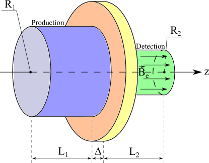
Figure 2: A scheme for the setup considered. The detection cavity ($R_{2}$) is separated from the production cavity ($R_{1}$) by a screening plate of width $\Delta$.

The detection cavity response to the external axion field is determined by Eq. (3). The latter one decouples into a pair of Maxwell’s equations with axion-induced current,

$$(\vec{\nabla}\cdot\vec{E})=-g_{a\gamma\gamma}\,(\vec{B}\cdot\vec{\nabla}\,a)\;,\qquad\qquad[\vec{\nabla}\times\vec{B}]=\frac{\partial}{\partial t}\vec{E}+g_{a\gamma\gamma}\left(\vec{B}\frac{\partial}{\partial t}a-[\vec{E}\times\vec{\nabla}\,a]\right)\;.$$ (20)

The electric field of a given signal mode $\vec{E}^{\mathrm{sig}}(\vec{x},t)$ inside the detection cavity obeys the following equation

$$\left(\frac{\partial^{2}}{\partial t^{2}}+\Gamma\frac{\partial}{\partial t}-\Delta\right)\vec{E}^{\mathrm{sig}}(\vec{x},t)=g_{a\gamma\gamma}\left(\vec{\nabla}\,(\vec{B}_{e}(\vec{x})\cdot\vec{\nabla}\,a(\vec{x},t))-\vec{B}_{e}(\vec{x})\frac{\partial^{2}}{\partial t^{2}}a(\vec{x},t)\right),$$ (21)

where we introduced the damping coefficient $\Gamma$ to take into account dissipation effects; r.h.s is associated with the ALPs and magnetic field $\vec{B}_{e}(\vec{x})$ inside the cavity.

Next, to simplify our considerations we take uniform magnetic field $\vec{B}_{e}$ directed along $z$ axis inside the cavity. We use a mode expansion for the signal electric field inside the detection cavity,

$$\vec{E}^{\mathrm{sig}}(\vec{x},t)=\sum_{m}\vec{{\cal E}}_{m}(\vec{x})E^{\mathrm{sig}}_{m}(t)\;,$$ (22)

where $\vec{{\cal E}}_{m}(\vec{x})$ are cavity eigenmodes with fixed normalization,

$$\Delta\,\vec{{\cal E}}_{m}(\vec{x})+\omega_{m}^{2}\vec{{\cal E}}_{m}(\vec{x})=0\;,\qquad\qquad\int\limits_{\mathrm{2\,cav}}d^{3}x\,(\vec{{\cal E}}_{m}(\vec{x})\cdot\vec{{\cal E}}_{n}(\vec{x}))=V_{2}\cdot\delta_{mn}\;,$$ (23)

satisfying necessary boundary conditions. We note that index $m$ accounts for $n,\,p,\,q$ winding numbers of the cavity. The integration in (23) is performed over the volume of the detection cavity $V_{2}$. Since the signal modes are orthogonal, one obtains the following equation by substituting (22) into (21) and multiplying each cavity mode by $\vec{{\cal E}}_{m}(\vec{x})$,

$$\left(\frac{\partial^{2}}{\partial t^{2}}+\Gamma\frac{\partial}{\partial t}+\omega_{m}^{2}\right)E_{m}^{\mathrm{sig}}(t)=-g_{a\gamma\gamma}\int\limits_{\mathrm{2\,cav}}\frac{d^{3}x}{V_{2}}\left[(\vec{{\cal E}}_{m}(\vec{x})\cdot\vec{B}_{e})\,\ddot{a}(\vec{x},t)-\left(\vec{{\cal E}}_{m}(\vec{x})\cdot\left(\vec{B}_{e}\vec{\nabla}\right)\vec{\nabla}a(\vec{x},t)\right)\right]\;,$$ (24)

where the r.h.s is an axion-induced driven force. The second term in the r.h.s. of (24) is suppressed compared to the first one if the produced axions are non-relativistic. However, in the general case these two terms seem to be of the same order. Since the magnetic field in the detection cavity $\vec{B}_{e}$ is directed along $z$ axis, the scalar product $(\vec{{\cal E}}_{m}(\vec{x})\cdot\vec{B}_{e})$ does not vanish if only ${\cal E}^{z}_{m}$ does not depend on $z$, or the winding number for the detection mode $q=0$. Moreover, it is more convenient to use the detection mode TM010. For that mode the only nonzero component is ${\cal E}^{z}_{m}$. The corresponding electric field, including normalization factor, reads ${\cal E}^{z}_{TM010}(\vec{x})=1.92\,J_{0}\left(\dfrac{x_{01}}{a}\rho\right)$. Thus, (24) simplifies,

$$\left(\frac{\partial^{2}}{\partial t^{2}}+\Gamma\frac{\partial}{\partial t}+\omega_{m}^{2}\right)E_{m}^{\mathrm{sig}}(t)=-g_{a\gamma\gamma}B_{e}^{z}\int\limits_{\mathrm{2\,cav}}\frac{d^{3}x}{V_{2}}{\cal E}_{m}^{z}(\vec{x})\,\left(\ddot{a}(\vec{x},t)-\partial_{z}^{2}a(\vec{x},t)\right)\,,$$ (25)

If the r.h.s. of Eq. (25) oscillates as $e^{-i\omega t}$, the complex solution of Eq. (25) reads the r.h.s. multiplied to $(-\omega^{2}-i\omega\Gamma+\omega_{m}^{2})^{-1}$. This is exactly the case of aforementioned produced axion field determined by Eqs. (6) and (7). For $m_{a}<\omega_{\pm}$ the signal electric field $E_{m}^{\mathrm{sig}}(t)$ reads

$$E_{m}^{\mathrm{sig}}(t)=\frac{-g_{a\gamma\gamma}^{2}B_{e}^{z}}{\omega_{\pm}^{2}-\omega_{m}^{2}+i\omega_{\pm}\Gamma}\int\limits_{\mathrm{2\,cav}}\frac{d^{3}x}{V_{2}}{\cal E}_{m}^{z}(\vec{x})\,\int\limits_{\mathrm{1\,cav}}d^{3}x^{\prime}\frac{F_{\pm}(x^{\prime})}{4\pi}\left(\omega_{\pm}^{2}+\partial_{z}^{2}\right)\frac{\mathrm{e}^{-i\omega_{\pm}t+ik_{\pm}|x-x^{\prime}|}}{|x-x^{\prime}|}\;.$$ (26)

The signal field $E_{m}^{\mathrm{sig}}(t)$ has a narrow peak at $\omega_{m}\simeq\omega_{\pm}$. The frequency $\omega_{m}$ of cavity detection eigenmode can be adjusted to a value $\omega_{m}\simeq\omega_{\pm}$ by fixing the radius $R_{2}$ of the detection cavity. The damping coefficient $\Gamma$ can be expressed via the quality factor $Q$ of the detection cavity, $\Gamma=\omega_{m}/Q$. Thus, averaged squared amplitude for electric field of the signal mode reads

$$\langle|E_{m}^{\mathrm{sig}}(t)|^{2}\rangle\equiv 1/2\left(E^{\pm c}_{m}\right)^{2}+1/2\left(E^{\pm s}_{m}\right)^{2}\;,$$ (27)

where

$$E^{\mathrm{\pm c(s)}}_{m}=\frac{g_{a\gamma\gamma}^{2}E_{0}^{2}Q{B}^{z}_{c}}{4\pi}\cdot\frac{V_{\mathrm{1\,cav}}}{\Delta}\cdot\kappa_{m}^{\pm c(s)},\qquad\kappa_{m}^{\pm c(s)}=\left(\alpha^{\mathrm{\pm c(s)}}_{m}+\frac{\beta^{\mathrm{\pm c(s)}}_{m}}{\omega_{\pm}^{2}L_{1}^{2}}\right)\;,$$ (28)

and $\Delta$ is a distance between borders of two cavities (see Fig. 3), and $\alpha^{\mathrm{\pm c(s)}}_{m}$ and $\beta^{\mathrm{\pm c(s)}}_{m}$ are dimensionless geometrical form-factors,

$$\alpha^{\mathrm{\pm c(s)}}_{m}=\int\limits_{\mathrm{2\,cav}}\frac{d^{3}x}{V_{2}}\,{\cal E}^{z}_{m}(\vec{x})\int\limits_{\mathrm{1\,cav}}\frac{d^{3}x^{\prime}}{V_{1}}\frac{\left|F_{\pm}(\vec{x}\,^{\prime})\right|}{E_{0}^{2}}\cdot\frac{\Delta}{|\vec{x}-\vec{x}^{\prime}|}\left\{\begin{array}[]{c}\cos\left(k_{\pm}|\vec{x}-\vec{x}^{\prime}|\right)\\ \sin\left(k_{\pm}|\vec{x}-\vec{x}^{\prime}|\right)\end{array}\right\},$$ (29)

$$\beta^{\mathrm{\pm c(s)}}_{m} = \int\limits_{\mathrm{2\,cav}}\frac{d^{3}x}{V_{2}}\,{\cal E}^{z}_{m}(\vec{x})\int\limits_{\mathrm{1\,cav}}\frac{d^{3}x^{\prime}}{V_{1}}\frac{\partial^{2}_{z^{\prime}}\left|F_{\pm}(\vec{x}\,^{\prime})\right|}{E_{0}^{2}}\cdot\frac{\Delta\cdot L_{1}^{2}}{|\vec{x}-\vec{x}^{\prime}|}\left\{\begin{array}[]{c}\cos\left(k_{\pm}|\vec{x}-\vec{x}^{\prime}|\right)\\ \sin\left(k_{\pm}|\vec{x}-\vec{x}^{\prime}|\right)\end{array}\right\}-$$ (32)

$$- \int\limits_{\mathrm{2\,cav}}\dfrac{d^{3}x}{V_{2}}\,{\cal E}^{z}_{m}(\vec{x})\int\limits_{\mathrm{1\,S}}\dfrac{\rho^{\prime}d\rho^{\prime}d\varphi^{\prime}}{V_{1}}\dfrac{\partial_{z^{\prime}}|F_{\pm}(\vec{x^{\prime}})|}{E_{0}^{2}}\cdot\dfrac{\Delta\cdot L_{1}^{2}}{|\vec{x}-\vec{x}^{\prime}|}\left\{\begin{array}[]{c}\cos\left(k_{\pm}|\vec{x}-\vec{x}^{\prime}|\right)\\ \sin\left(k_{\pm}|\vec{x}-\vec{x}^{\prime}|\right)\end{array}\right\}\bigg{|}_{z^{\prime}=0}^{z^{\prime}=L}\;.$$ (35)

In deriving the expression (35) for simplicity of numerical calculations we transferred the derivative over $z$ to $z^{\prime}$. The last term of Eq. (35) appeared as the result of integrating by parts, see Appendix C for details.

We estimate the number of signal photons for a given mode in receiving cavity as follows [1],

$$N_{s}\simeq\frac{1}{2\omega}\int\limits_{\mathrm{2\,cav}}d^{3}x\,\langle|\vec{E}^{\mathrm{sig}}(\vec{x},t)|^{2}\rangle\simeq\frac{V_{2}}{2\omega}\langle|E_{m}^{\mathrm{sig}}(t)|^{2}\rangle\;.$$ (36)

Signal-to-noise ratio has the following form [33],

$$\text{SNR}\simeq\frac{N_{s}}{N_{\mathrm{th}}}\frac{1}{2L_{2}Q}\sqrt{\frac{t}{B}}\;,$$ (37)

where $t$ is a time of measurement, $B$ is a bandwidth of the signal, $L_{2}$ is a receiving cavity length, $N_{\mathrm{th}}=T/\omega$ is a number of thermal photons at $T\gg\omega$. One has the following limit on coupling,

$$g_{a\gamma\gamma}\simeq\left(\frac{128\pi^{2}TL_{2}\Delta^{2}}{E_{0}^{4}(B^{z}_{c})^{2}Q((\kappa_{m}^{c+})^{2}+(\kappa_{m}^{s+})^{2})V_{1}^{2}V_{2}}\sqrt{\frac{B}{t}}\text{SNR}\right)^{1/4}\;.$$ (38)

However, the volume of detecting cavity $V_{2}=\pi R_{2}^{2}\cdot L_{2}$ is not an independent variable for fixed detection mode. The resonant condition $\omega_{TM010}=\omega_{\pm}$ for detection with TM010 mode yields $R_{2}=x_{01}/\omega_{\pm}$. Thus, we have

$$g_{a\gamma\gamma}\simeq 2.52\left(\frac{T\cdot\Delta^{2}\,\cdot\,\omega_{\pm}^{2}}{E_{0}^{4}(B^{z}_{c})^{2}Q((\kappa_{m}^{c+})^{2}+(\kappa_{m}^{s+})^{2})V_{1}^{2}}\sqrt{\frac{B}{t}}\text{SNR}\right)^{1/4}\;.$$ (39)

In particular, Eq. (39) can be expressed as

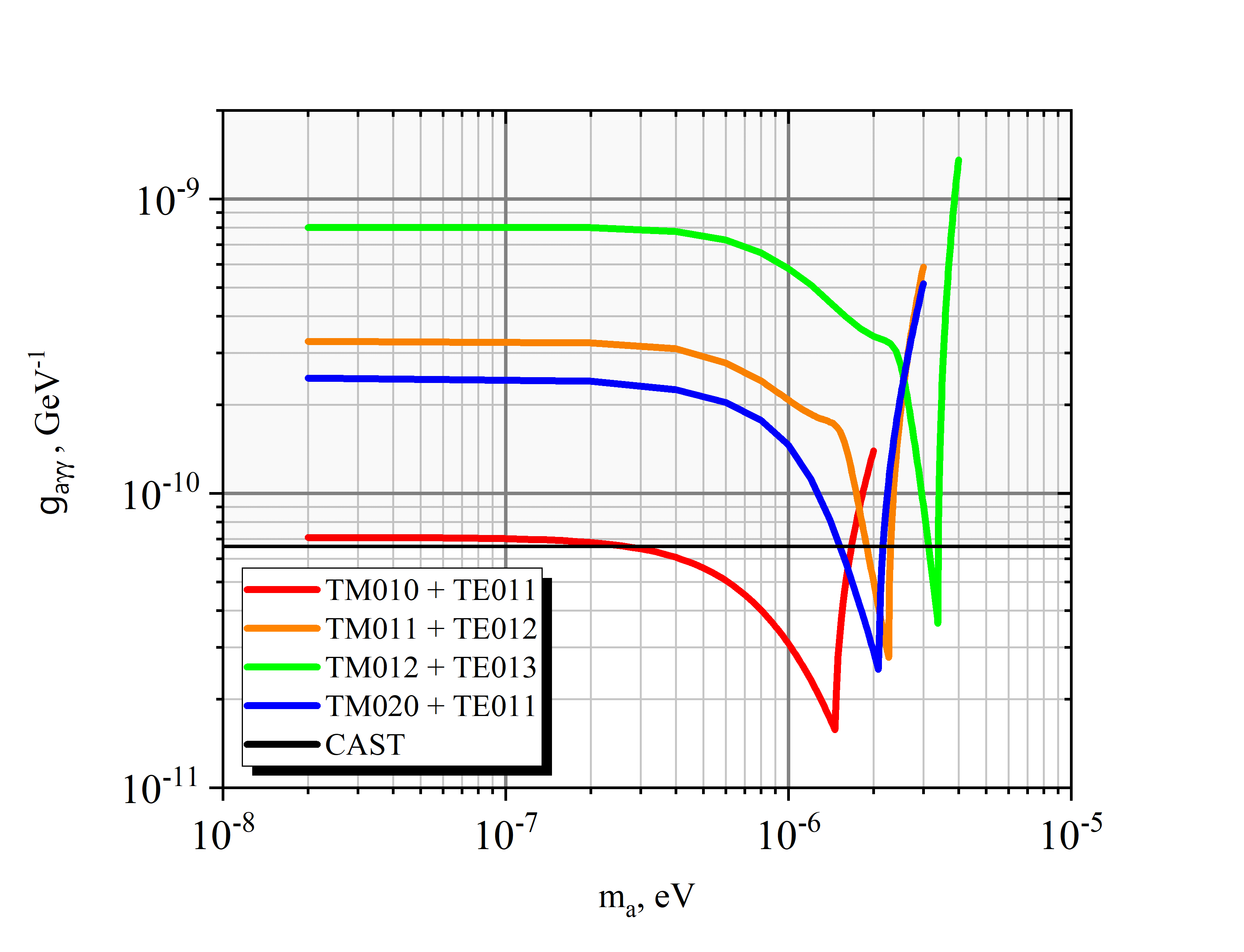
Figure 3: Projected sensitivity of the proposed setup to ALP mass $m_{a}$ and $g_{a\gamma\gamma}$ parameter for different sets of pump modes in the production cavity. The black line shows the solar axion constraint from CAST [6].

$$g_{a\gamma\gamma} \simeq 2.7\cdot 10^{-12}\,\mbox{GeV}^{-1}\left(\frac{T}{1.5\,\mbox{K}}\right)^{1/4}\left(\frac{\Delta}{0.2\,\mbox{m}}\right)^{1/2}\left(\frac{\omega_{\pm}}{1.5\,\cdot\,10^{-6}\,\mbox{eV}}\right)^{1/2}\left(\frac{V_{1}}{1\,\mbox{m}^{3}}\right)^{-1/2}\left(\frac{Q}{10^{5}}\right)^{-1/4}\times$$

$$\times\left(\left(\kappa_{c}^{+}\right)^{2}+\left(\kappa_{s}^{+}\right)^{2}\right)^{-1/4}\left(\frac{E_{0}}{0.1\,\mbox{T}}\right)^{-1}\left(\frac{B_{e}^{z}}{10\,\mbox{T}}\right)^{-1/2}\left(\frac{t}{10^{6}\,\mbox{sec}}\right)^{-1/8}\left(\frac{B}{1\,\mbox{Hz}}\right)^{1/8}\left(\frac{\mbox{SNR}}{5}\right)^{1/4}.$$ (40)

The constraints (4) at the parametric plane $(g_{a\gamma\gamma},m_{a})$ are shown in Fig. 3 for different sets of pump modes. The magnitudes of the external parameters, $T,\,\Delta,\,Q,\,E_{0},\,B_{e}^{z},\,t,\,B$ and SNR correspond to their typical values in brackets. The resonant constraints on $g_{a\gamma\gamma}$ for larger number of different pump mode combinations and for different ratio $R_{1}/L_{1}$ are shown in Table 1.

Let us discuss the parametric dependence in Eq. (4). First, these bounds are sensitive to the magnitude of the field $E_{0}$. In particular, factor $0.1$ in the amplitude implies suppression of the bound (4) by factor $10$. Second, the dependence on the linear sizes of the setup can be seen from Eq. (38). We note that dimensionless form-factors $\kappa_{c(s)}^{\pm}$ feebly depend on $V_{1}$ and $V_{2}$. Therefore, by increasing the linear sizes of the setup by factor of $2$ one can achieve the improved limit on $g_{a\gamma\gamma}$ by factor $2^{3/2}\simeq 2.8$.

5 Discussion

In the present paper we have calculated numerically the time-averaged axion energy density $\langle\rho^{E}\rangle$ generated by two electromagnetic modes in the superconducting cylindrical cavity. In particular, we have studied the spatial distribution of $\langle\rho^{E}\rangle$ for various axion masses and for different types of cylindrical cavity. We have shown numerically that there is a parametric resonance if axion produced in nonrelativistic regime for the frequency component $\omega_{+}=|\omega_{1}+\omega_{2}|$ and for certain combination of pump modes. On the contrary, for the frequency component $\omega_{-}=|\omega_{1}-\omega_{2}|$ there is no significant resonance in that regime.

Considering different combinations of pump modes in the production cavity we have shown that they may have different efficiency for axion production. In particular, the highest amplitude for the produced axion field came from TE$n_{1}p_{1}q_{1}$+TM$n_{2}p_{2}q_{2}$ modes with $n_{1}=n_{2}$ and even $q_{1}+q_{2}$. Concerning different radius-to-length ratio $R/L$ for the cavity, we have shown that for a “pancake-like” cavity, $L/R\lesssim 1$, the maximum ALP energy density outside the cavity is produced along the cylinder axis $z$. Otherwise, for “prolonged” design of the cavity, $L/R\gg 1$, the maximum energy density outside the cylinder is produced near the side surface (this case was studied in Ref. [35]).

We also discuss the detection of ALPs in the additional separated cavity, which is filled with the strong magnetic field. We estimated the projected sensitivity of the proposed setup on the ALPs parameter space $(m_{a},g_{a\gamma\gamma})$. We have shown that the best constraint came from the mode combination TM010+TE011 in the production cavity.

In addition, we have calculated the sensitivity curves for high order pump modes of the production cavity. The advantage of generating high order pump modes is that one can probe the region with higher masses of ALPs. However the peak sensitivity to the ALPs coupling is decreased in that case. Although the resonances at Fig. 3 are quite narrow, we can test larger area of parameters by exciting different set of high order pump modes. Nevertheless, for fixed cavity geometry there are still spaces between resonant peaks at the exclusion plot. One can modify eigenmodes by adjusting the geometry of given cavity. Therefore, the relevant unconstrained area can be probed.

Note that our setup can be easily generalized to other designs of the detection cavity. In particular, the analysis can be easily applied the toroidal detection cavity [35]. By exciting high order pump modes one can shift the resonant bounds of [35] to the area of higher ALP masses. Another interesting task is to consider parametric resonances for the single cavity which produces and detects ALPs [33]. I addition, it is instructive to probe hidden photon [47] in SRF cavity. We leave these tasks for further work.

Acknowledgements

The authors thank Sergey Troitsky, Dmitry Levkov, Alexander Panin, Ilya Kopchinskii, Yuri Senichev, Leonid Kravchuk, Valentin Paramonov, Andrey Egorov, Leonid Kuzmin and Andrey Pankratov for helpful discussions. Numerical calculations were performed on the Computational Cluster of the Theoretical division of INR RAS. The work of P.S. and M.F. was supported by RSF grant 18-12-00258.

Appendix A Retarded Green function

In this Appendix we show some details of deriving Eqs. (6), (7). The Klein-Gordon’s retarded Green function can be written as follows [48],

$$G_{\mathrm{ret}}(\vec{x},\vec{x}^{\prime},t,t^{\prime})=\frac{1}{4\pi}\Bigl{(}\frac{\delta(t-t^{\prime}-R)}{R}-\theta(t-t^{\prime}-R)\frac{m_{a}}{u}J_{1}(m_{a}u)\Bigr{)}\;,$$ (41)

where $u\equiv\sqrt{(t-t^{\prime})^{2}-R^{2}}$ and $R\equiv|\vec{x}-\vec{x}^{\prime}|$. The first term in Eq. (41) describes the retarded Green function of the massless scalar field, so that the mass dependence is only in the second term. In Eq. (4) the retarded Green function should be integrated over $t^{\prime}$ with the electromagnetic invariant $\vec{E}(x^{\prime},t^{\prime})\cdot\vec{B}(x^{\prime},t^{\prime})$. For considered modes $t^{\prime}$ dependence decouples as $e^{-i\omega t^{\prime}}$. For purpose of integration of the second term of Eq. (41) the textbook integral [49] can be used,

$$\int\limits_{R}^{\infty}d\tilde{t}\,\frac{\mathrm{e}^{i\omega\tilde{t}}}{\sqrt{\tilde{t}^{2}-R^{2}}}J_{1}(m_{a}\sqrt{\tilde{t}^{2}-R^{2}})=\frac{1}{m_{a}R}\left(\mathrm{e}^{iR\omega}-\mathrm{e}^{iR\sqrt{\omega^{2}-m_{a}^{2}}}\right)\;.$$ (42)

Integrating the Green function (41), one obtains

$$\int\limits^{t-R}_{-\infty}dt^{\prime}\,G_{\mathrm{ret}}(\vec{x},\vec{x}^{\prime},t,t^{\prime})\,\mathrm{e}^{-i\omega t^{\prime}}=\frac{1}{4\pi R}\,\mathrm{e}^{-i\omega t+iRk}\;,$$ (43)

where $k=\sqrt{\omega^{2}-m_{a}^{2}}$. If $m_{a}<\omega$, $ik$ should be replaced by $\kappa=\sqrt{m_{a}^{2}-\omega^{2}}$. As a result, one immediately obtains Eqs. (6), (7).

Appendix B Exact form of $TM_{npq}$ and $TE_{npq}$ modes

$TM_{npq}$ and $TE_{npq}$ modes are expressed in terms of the electric and magnetic fields [42] as

$${\cal E}^{TMnpq}_{z} ={\cal E}_{0}J_{n}\left(\dfrac{x_{np}}{R}\rho\right)\left\{\begin{array}[]{c}\sin n\varphi\\ \cos n\varphi\end{array}\right\}\cos\left(\dfrac{q\pi}{L}z\right),$$ (46)

$${\cal E}^{TMnpq}_{\rho} =\dfrac{-{\cal E}_{0}}{k^{2}_{npq}-(q\pi/L)^{2}}\cdot\dfrac{q\pi}{L}\cdot\dfrac{x_{np}}{R}\cdot J^{\prime}_{n}\left(\dfrac{x_{np}}{R}\rho\right)\left\{\begin{array}[]{c}\sin n\varphi\\ \cos n\varphi\end{array}\right\}\sin\left(\dfrac{q\pi}{L}z\right),$$ (49)

$${\cal E}^{TMnpq}_{\varphi} =\dfrac{-{\cal E}_{0}}{k^{2}_{npq}-(q\pi/L)^{2}}\cdot\dfrac{1}{\rho}\cdot\dfrac{nq\pi}{L}\cdot J_{n}\left(\dfrac{x_{np}}{R}\rho\right)\left\{\begin{array}[]{c}\cos n\varphi\\ -\sin n\varphi\end{array}\right\}\sin\left(\dfrac{q\pi}{L}z\right),$$ (52)

$${\cal B}^{TMnpq}_{z} =0,$$ (53)

$${\cal B}^{TMnpq}_{\rho} =\dfrac{-i\omega^{TM}_{npq}{\cal E}_{0}}{k^{2}_{npq}-(q\pi/L)^{2}}\cdot\dfrac{n}{\rho}\cdot J_{n}\left(\dfrac{x_{np}}{R}\rho\right)\left\{\begin{array}[]{c}\cos n\varphi\\ -\sin n\varphi\end{array}\right\}\cos\left(\dfrac{q\pi}{L}z\right),$$ (56)

$${\cal B}^{TMnpq}_{\varphi} =\dfrac{i\omega^{TM}_{npq}{\cal E}_{0}}{k^{2}_{npq}-(q\pi/L)^{2}}\cdot\dfrac{x_{np}}{R}\cdot J^{\prime}_{n}\left(\dfrac{x_{np}}{R}\rho\right)\left\{\begin{array}[]{c}\sin n\varphi\\ \cos n\varphi\end{array}\right\}\cos\left(\dfrac{q\pi}{L}z\right);$$ (59)

$${\cal B}^{TEnpq}_{z} ={\cal B}_{0}J_{n}\left(\dfrac{x^{\prime}_{np}}{R}\rho\right)\left\{\begin{array}[]{c}\sin n\varphi\\ \cos n\varphi\end{array}\right\}\sin\left(\dfrac{q\pi}{L}z\right),$$ (62)

$${\cal B}^{TEnpq}_{\rho} =\dfrac{{\cal B}_{0}}{k^{2}_{npq}-(q\pi/L)^{2}}\cdot\dfrac{q\pi}{L}\cdot\dfrac{x^{\prime}_{np}}{R}\cdot J^{\prime}_{n}\left(\dfrac{x^{\prime}_{np}}{R}\rho\right)\left\{\begin{array}[]{c}\sin n\varphi\\ \cos n\varphi\end{array}\right\}\cos\left(\dfrac{q\pi}{L}z\right),$$ (65)

$${\cal B}^{TEnpq}_{\varphi} =\dfrac{{\cal B}_{0}}{k^{2}_{npq}-(q\pi/L)^{2}}\cdot\dfrac{1}{\rho}\cdot\dfrac{nq\pi}{L}\cdot J_{n}\left(\dfrac{x^{\prime}_{np}}{R}\rho\right)\left\{\begin{array}[]{c}\cos n\varphi\\ -\sin n\varphi\end{array}\right\}\cos\left(\dfrac{q\pi}{L}z\right),$$ (68)

$${\cal E}^{TEnpq}_{z} =0,$$ (69)

$${\cal E}^{TEnpq}_{\rho} =\dfrac{i\omega^{TE}_{npq}{\cal B}_{0}}{k^{2}_{npq}-(q\pi/L)^{2}}\cdot\dfrac{n}{\rho}\cdot J_{n}\left(\dfrac{x^{\prime}_{np}}{R}\rho\right)\left\{\begin{array}[]{c}\cos n\varphi\\ -\sin n\varphi\end{array}\right\}\sin\left(\dfrac{q\pi}{L}z\right),$$ (72)

$${\cal E}^{TEnpq}_{\varphi} =\dfrac{-i\omega^{TE}_{npq}{\cal B}_{0}}{k^{2}_{npq}-(q\pi/L)^{2}}\cdot\dfrac{x^{\prime}_{np}}{R}\cdot J^{\prime}_{n}\left(\dfrac{x^{\prime}_{np}}{R}\rho\right)\left\{\begin{array}[]{c}\sin n\varphi\\ \cos n\varphi\end{array}\right\}\sin\left(\dfrac{q\pi}{L}z\right).$$ (75)

Appendix C The gradient of axion field

For the case $m_{a}<\omega_{\pm}$ let us calculate the axion field’s gradient (calculation for $m_{a}>\omega_{\pm}$ is similar). Using Eq. (6) and the relation $\vec{\nabla}_{x}\,f(|\vec{x}-\vec{x}^{\prime}|)=-\vec{\nabla}_{x^{\prime}}\,f(|\vec{x}-\vec{x}^{\prime}|)$ one finds

$$\vec{\nabla}a_{\pm}(\vec{x},t)=-g_{a\gamma\gamma}\;\Re\mathrm{e}\,\int\limits_{V_{\mathrm{cav}}}d^{3}x^{\prime}\,\frac{F_{\pm}(\vec{x}^{\prime})}{4\pi}\left\{-\vec{\nabla}_{x^{\prime}}\dfrac{\mathrm{e}^{-i\omega_{\pm}t+i|\vec{x}-\vec{x}^{\prime}|k_{\pm}}}{|\vec{x}-\vec{x}^{\prime}|}\right\}\;.$$ (76)

Next, integrating this equation by parts and using Stokes’ theorem one gets

$$\vec{\nabla}a_{\pm}(\vec{x},t) = -g_{a\gamma\gamma}\;\Re\mathrm{e}\,\int\limits_{V_{\mathrm{cav}}}d^{3}x^{\prime}\,\frac{\vec{\nabla}_{x^{\prime}}F_{\pm}(\vec{x}^{\prime})}{4\pi|\vec{x}-\vec{x}^{\prime}|}\mathrm{e}^{-i\omega_{\pm}t+i|\vec{x}-\vec{x}^{\prime}|k_{\pm}}\;+$$ (77)

$$+g_{a\gamma\gamma}\;\Re\mathrm{e}\,\oint\limits_{\partial V_{\mathrm{cav}}}\vec{n}\,d\sigma^{\prime}\,\dfrac{F_{\pm}(\vec{x}^{\prime})}{4\pi}\cdot\dfrac{\mathrm{e}^{-i\omega_{\pm}t+i|\vec{x}-\vec{x}^{\prime}|k_{\pm}}}{|\vec{x}-\vec{x}^{\prime}|}\;.$$

Direct substitution yields the condition $F_{\pm}(\vec{x}^{\prime})=0$ on the cavity walls. Therefore, the second term in the last formula is zero and we get

$$\vec{\nabla}a_{\pm}(\vec{x},t)=-g_{a\gamma\gamma}\;\Re\mathrm{e}\,\int\limits_{V_{\mathrm{cav}}}d^{3}x^{\prime}\,\frac{\vec{\nabla}_{x^{\prime}}F_{\pm}(\vec{x}^{\prime})}{4\pi|\vec{x}-\vec{x}^{\prime}|}\mathrm{e}^{-i\omega_{\pm}t+i|\vec{x}-\vec{x}^{\prime}|k_{\pm}}\;.$$ (78)

Let us derive the expression $\vec{\mathcal{E}}_{m}\cdot\vec{\nabla}\,(\vec{B}_{e}(\vec{x})\cdot\vec{\nabla}\,a(\vec{x},t))$ given the conditions $\vec{B}_{e}=B^{z}_{e}\cdot\vec{e}_{z}$, $B^{z}_{e}=\mathrm{const}$, and $\vec{\mathcal{E}}_{m}(\vec{x})=\mathcal{E}^{z}_{m}(\vec{x})\cdot\vec{e}_{z}$. Integrating by parts and taking into account that $\partial_{z^{\prime}}F_{\pm}(\vec{x}^{\prime})\neq 0$ on the cavity wall we arrive at the formula

$$\vec{\mathcal{E}}_{m}\cdot\vec{\nabla}(\vec{B}_{e}\cdot\vec{\nabla}a_{\pm}(\vec{x},t))=-g_{a\gamma\gamma}B^{z}_{e}\mathcal{E}^{z}_{m}(\vec{x})\;\Re\mathrm{e}\,\int\limits_{V_{\mathrm{cav}}}d^{3}x^{\prime}\,\frac{\partial^{2}_{z^{\prime}}F_{\pm}(\vec{x}^{\prime})}{4\pi|\vec{x}-\vec{x}^{\prime}|}\mathrm{e}^{-i\omega_{\pm}t+i|\vec{x}-\vec{x}^{\prime}|k_{\pm}}\;+$$

$$+g_{a\gamma\gamma}B^{z}_{e}\mathcal{E}^{m}_{z}(\vec{x})\;\Re\mathrm{e}\,\int\limits_{\partial V_{\mathrm{cav}}}\rho^{\prime}d\rho^{\prime}d\varphi^{\prime}\,\frac{\partial_{z^{\prime}}F_{\pm}(\vec{x}^{\prime})}{4\pi|\vec{x}-\vec{x}^{\prime}|}\mathrm{e}^{-i\omega_{\pm}t+i|\vec{x}-\vec{x}^{\prime}|k_{\pm}}\bigg{|}_{z^{\prime}=0}^{z^{\prime}=L}\;.$$ (79)

Taking out dimensionful values, one comes to (35).

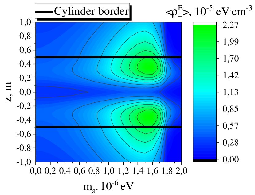
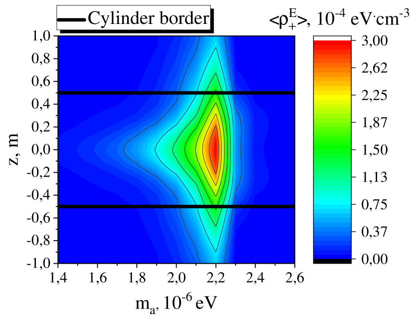
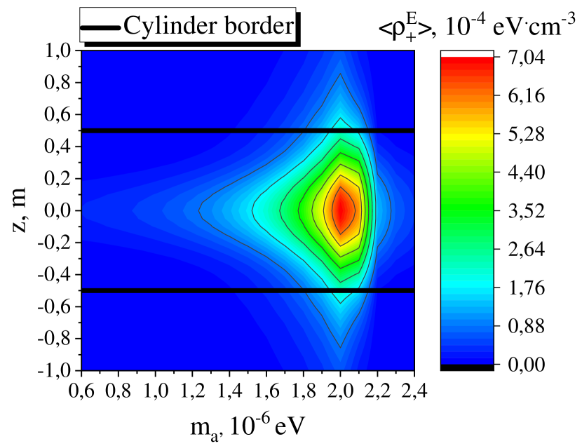
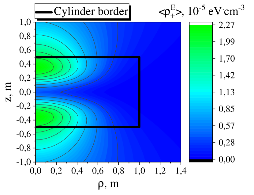
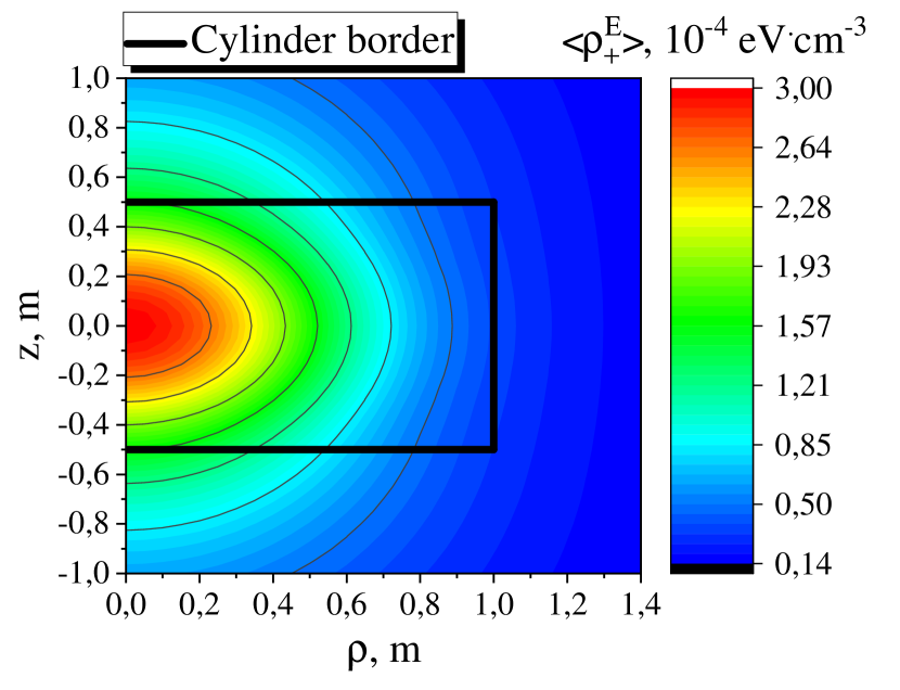
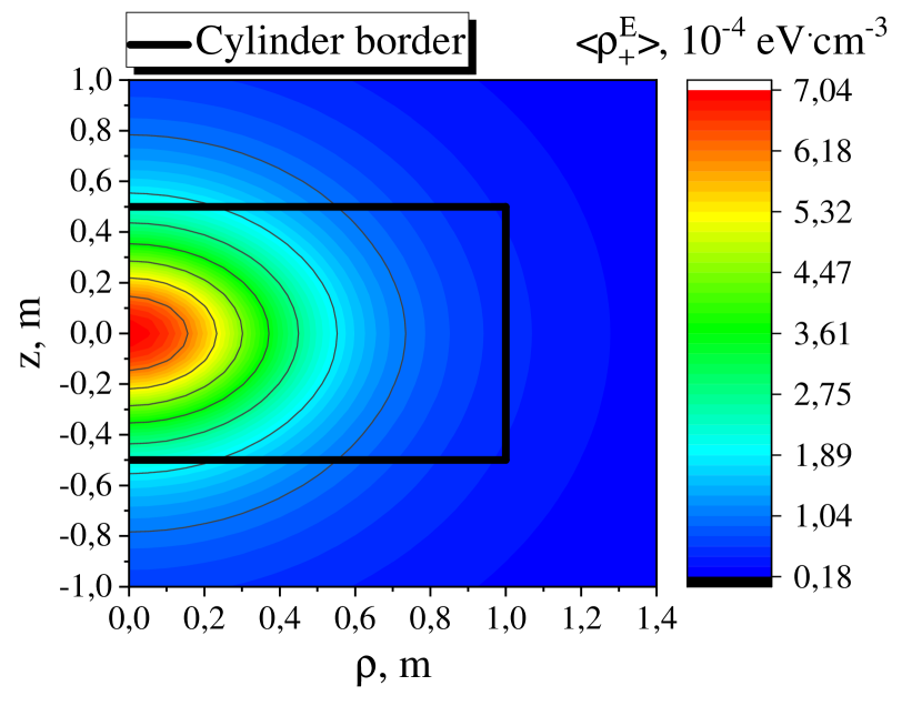
Figure 4: Contour plot for the time-averaged energy density $\braket{\rho^{E}_{+}}$ evaluated on the cylinder axis as function of axion mass $m_{a}$ and the distance $z$ from center of cavity (left panels) and spatial distribution of $\braket{\rho^{E}_{+}}$ on the cavity section along its axis $(\rho,\,z)$ (right panels) with TM011+TE011 $\omega_{+}=17.8\cdot 10^{-7}$ eV (top), TM011+TE012 $\omega_{+}=22.6\cdot 10^{-7}$ eV (middle), and TM020+TE011 $\omega_{+}=21.0\cdot 10^{-7}$ eV (bottom) pump modes. Cavity dimensions: $L=1$ m, $R=1$ m.

Cavities parameters						$\kappa_{c}$	$g_{a\gamma\gamma},\mathrm{GeV}^{-1}$
$R_{1},\mathrm{m}$	$L_{1},\mathrm{m}$	Prod. modes	$\omega_{+},\mathrm{eV}$	$R_{2},\mathrm{m}$
$1$	$1$	TM010+TE011	$1.47\cdot 10^{-6}$	$0.33$		$9.71\cdot 10^{-3}$	$1.55\cdot 10^{-11}$
		TM011+TE012	$2.26\cdot 10^{-6}$	$0.21$		$4.72\cdot 10^{-3}$	$2.75\cdot 10^{-11}$
		TM012+TE013	$3.38\cdot 10^{-6}$	$0.14$		$4.07\cdot 10^{-3}$	$3.62\cdot 10^{-11}$
		TM020+TE011	$2.10\cdot 10^{-6}$	$0.23$		$5.45\cdot 10^{-3}$	$2.46\cdot 10^{-11}$
		TM011+TE011	$1.78\cdot 10^{-6}$	$0.27$		$6.60\cdot 10^{-4}$	$6.53\cdot 10^{-11}$
		TM021+TE011	$2.26\cdot 10^{-6}$	$0.21$		$5.87\cdot 10^{-4}$	$7.79\cdot 10^{-11}$
		TM021+TE021	$2.81\cdot 10^{-6}$	$0.17$		$7.42\cdot 10^{-4}$	$7.72\cdot 10^{-11}$
		TM013+TE014	$4.57\cdot 10^{-6}$	$0.11$		$3.89\cdot 10^{-3}$	$4.30\cdot 10^{-11}$
		TM013+TE015	$5.18\cdot 10^{-6}$	$0.09$		$7.88\cdot 10^{-4}$	$1.02\cdot 10^{-10}$
		TM110+TE111	$1.49\cdot 10^{-6}$	$0.32$		$2.85\cdot 10^{-2}$	$2.88\cdot 10^{-11}$
$2$	$0.25$	TM010+TE011	$2.78\cdot 10^{-6}$	$0.17$		$3.61\cdot 10^{-3}$	$3.49\cdot 10^{-11}$
		TM011+TE012	$7.57\cdot 10^{-6}$	$0.06$		$3.01\cdot 10^{-3}$	$6.29\cdot 10^{-11}$
		TM012+TE013	$1.26\cdot 10^{-5}$	$0.04$		$3.00\cdot 10^{-3}$	$8.14\cdot 10^{-11}$
		TM020+TE011	$3.09\cdot 10^{-6}$	$0.16$		$2.16\cdot 10^{-3}$	$4.76\cdot 10^{-11}$
		TM011+TE011	$5.07\cdot 10^{-6}$	$0.09$		$2.60\cdot 10^{-6}$	$1.75\cdot 10^{-9}$
		TM021+TE011	$5.12\cdot 10^{-6}$	$0.09$		$4.67\cdot 10^{-6}$	$1.31\cdot 10^{-9}$
		TM021+TE021	$5.18\cdot 10^{-6}$	$0.09$		$7.20\cdot 10^{-6}$	$1.07\cdot 10^{-9}$
		TM013+TE014	$1.76\cdot 10^{-5}$	$0.03$		$2.99\cdot 10^{-3}$	$9.63\cdot 10^{-11}$
		TM013+TE015	$2.01\cdot 10^{-5}$	$0.02$		$7.01\cdot 10^{-5}$	$6.72\cdot 10^{-10}$
		TM110+TE111	$2.90\cdot 10^{-6}$	$0.17$		$1.65\cdot 10^{-3}$	$5.26\cdot 10^{-11}$
$0.5$	$4$	TM010+TE011	$2.50\cdot 10^{-6}$	$0.19$		$4.53\cdot 10^{-3}$	$2.95\cdot 10^{-11}$
		TM011+TE012	$2.54\cdot 10^{-6}$	$0.19$		$3.66\cdot 10^{-3}$	$3.31\cdot 10^{-11}$
		TM012+TE013	$2.62\cdot 10^{-6}$	$0.18$		$3.35\cdot 10^{-3}$	$3.51\cdot 10^{-11}$
		TM020+TE011	$3.75\cdot 10^{-6}$	$0.13$		$2.52\cdot 10^{-3}$	$4.84\cdot 10^{-11}$
		TM011+TE011	$2.52\cdot 10^{-6}$	$0.19$		$1.18\cdot 10^{-3}$	$5.79\cdot 10^{-11}$
		TM021+TE011	$3.75\cdot 10^{-6}$	$0.13$		$6.69\cdot 10^{-4}$	$9.41\cdot 10^{-11}$
		TM021+TE021	$5.02\cdot 10^{-6}$	$0.10$		$7.47\cdot 10^{-4}$	$1.03\cdot 10^{-10}$
		TM013+TE014	$2.73\cdot 10^{-6}$	$0.18$		$3.23\cdot 10^{-3}$	$3.65\cdot 10^{-11}$
		TM013+TE015	$2.79\cdot 10^{-6}$	$0.17$		$1.91\cdot 10^{-3}$	$4.81\cdot 10^{-11}$
		TM110+TE111	$2.29\cdot 10^{-6}$	$0.21$		$1.47\cdot 10^{-3}$	$4.96\cdot 10^{-11}$

Table 1: Resonant sensitivities for $g_{a\gamma\gamma}$ for different combinations of pump modes. $R_{2}$ is the radius of detecting cavity. $g_{a\gamma\gamma}$ is the detectable lower bound.

References

• [1] I. G. Irastorza and J. Redondo, “New experimental approaches in the search for axion-like particles,” Prog. Part. Nucl. Phys. 102 (2018), 89-159 [arXiv:1801.08127 [hep-ph]].
• [2] R. D. Peccei and H. R. Quinn, “CP Conservation in the Presence of Instantons,” Phys. Rev. Lett. 38 (1977), 1440-1443.
• [3] R. D. Peccei and H. R. Quinn, “Constraints Imposed by CP Conservation in the Presence of Instantons,” Phys. Rev. D 16 (1977), 1791-1797.
• [4] P. Svrcek and E. Witten, “Axions In String Theory,” JHEP 06 (2006), 051 [arXiv:hep-th/0605206 [hep-th]].
• [5] A. Arvanitaki, S. Dimopoulos, S. Dubovsky, N. Kaloper and J. March-Russell, “String Axiverse,” Phys. Rev. D 81 (2010), 123530 [arXiv:0905.4720 [hep-th]].
• [6] V. Anastassopoulos et al. [CAST], Nature Phys. 13 (2017), 584-590 [arXiv:1705.02290 [hep-ex]].
• [7] Y. Kahn, B. R. Safdi and J. Thaler, Phys. Rev. Lett. 117 (2016) no.14, 141801 [arXiv:1602.01086 [hep-ph]].
• [8] S. J. Asztalos et al. [ADMX], Phys. Rev. D 64 (2001), 092003
• [9] D. F. Jackson Kimball, S. Afach, D. Aybas, J. W. Blanchard, D. Budker, G. Centers, M. Engler, N. L. Figueroa, A. Garcon and P. W. Graham, et al. Springer Proc. Phys. 245 (2020), 105-121 [arXiv:1711.08999 [physics.ins-det]].
• [10] A. Spector [ALPS], [arXiv:1906.09011 [physics.ins-det]].
• [11] H. B. Tran Tan, V. V. Flambaum, I. B. Samsonov, Y. V. Stadnik and D. Budker, Phys. Dark Univ. 24 (2019), 100272 [arXiv:1803.09388 [hep-ph]].
• [12] A. E. Egorov, N. P. Topchiev, A. M. Galper, O. D. Dalkarov, A. A. Leonov, S. I. Suchkov and Y. T. Yurkin, JCAP 2011 (2020) 049 [arXiv:2005.09032 [astro-ph.HE]].
• [13] J. L. Feng, I. Galon, F. Kling and S. Trojanowski, Phys. Rev. D 98 (2018) no.5, 055021 [arXiv:1806.02348 [hep-ph]].
• [14] A. Berlin, N. Blinov, G. Krnjaic, P. Schuster and N. Toro, Phys. Rev. D 99 (2019) no.7, 075001 [arXiv:1807.01730 [hep-ph]].
• [15] R. R. Dusaev, D. V. Kirpichnikov and M. M. Kirsanov, Phys. Rev. D 102, no. 5, 055018 (2020) [arXiv:2004.04469 [hep-ph]].
• [16] D. Banerjee et al. [NA64 Collaboration], Phys. Rev. Lett.  125 (2020) no.8, 081801 [arXiv:2005.02710 [hep-ex]].
• [17] V. Brdar, B. Dutta, W. Jang, D. Kim, I. M. Shoemaker, Z. Tabrizi, A. Thompson and J. Yu, arXiv:2011.07054 [hep-ph].
• [18] J. B. Dent, B. Dutta, D. Kim, S. Liao, R. Mahapatra, K. Sinha and A. Thompson, Phys. Rev. Lett. 124 (2020) no.21, 211804 [arXiv:1912.05733 [hep-ph]].
• [19] J. Preskill, M. B. Wise and F. Wilczek, Phys. Lett. B 120 (1983), 127-132 doi:10.1016/0370-2693(83)90637-8
• [20] L. F. Abbott and P. Sikivie, Phys. Lett. B 120 (1983), 133-136 doi:10.1016/0370-2693(83)90638-X
• [21] M. Dine and W. Fischler, Phys. Lett. B 120 (1983), 137-141 doi:10.1016/0370-2693(83)90639-1
• [22] Z. G. Berezhiani and M. Y. Khlopov, Z. Phys. C 49 (1991) 73. doi:10.1007/BF01570798
• [23] Z. G. Berezhiani, A. S. Sakharov and M. Y. Khlopov, Sov. J. Nucl. Phys.  55 (1992) 1063 [Yad. Fiz.  55 (1992) 1918].
• [24] C. J. Hogan and M. J. Rees, Phys. Lett. B 205 (1988), 228-230 doi:10.1016/0370-2693(88)91655-3
• [25] E. W. Kolb and I. I. Tkachev, Phys. Rev. Lett. 71 (1993), 3051-3054 doi:10.1103/PhysRevLett.71.3051 [arXiv:hep-ph/9303313 [hep-ph]].
• [26] A. Vilenkin, Phys. Rept. 121 (1985), 263-315 doi:10.1016/0370-1573(85)90033-X
• [27] A. S. Sakharov and M. Y. Khlopov, Phys. Atom. Nucl.  57 (1994) 485 [Yad. Fiz.  57 (1994) 514].
• [28] A. S. Sakharov, D. D. Sokoloff and M. Y. Khlopov, Phys. Atom. Nucl.  59 (1996) 1005 [Yad. Fiz.  59N6 (1996) 1050].
• [29] M. Colpi, S. L. Shapiro and I. Wasserman, Phys. Rev. Lett. 57 (1986), 2485-2488 doi:10.1103/PhysRevLett.57.2485
• [30] I. I. Tkachev, Phys. Lett. B 261 (1991), 289-293 doi:10.1016/0370-2693(91)90330-S
• [31] D. G. Levkov, A. G. Panin and I. I. Tkachev, Phys. Rev. D 102 (2020), 023501 [arXiv:2004.05179 [astro-ph.CO]].
• [32] J. H. Buckley, P. S. B. Dev, F. Ferrer and F. P. Huang, [arXiv:2004.06486 [astro-ph.HE]].
• [33] Z. Bogorad, A. Hook, Y. Kahn and Y. Soreq, “Probing Axionlike Particles and the Axiverse with Superconducting Radio-Frequency Cavities,” Phys. Rev. Lett.  123 (2019) no.2, 021801 [arXiv:1902.01418 [hep-ph]].
• [34] F. Hoogeveen, “Terrestrial axion production and detection using RF cavities,” Phys. Lett. B 288 (1992) 195.
• [35] R. Janish, V. Narayan, S. Rajendran and P. Riggins, “Axion production and detection with superconducting RF cavities,” Phys. Rev. D 100 (2019) no.1, 015036 [arXiv:1904.07245 [hep-ph]].
• [36] C. Gao and R. Harnik, “Axion Searches with Two Superconducting Radio-frequency Cavities,” [arXiv:2011.01350 [hep-ph]].
• [37] K. Van Bibber, N. R. Dagdeviren, S. E. Koonin, A. Kerman and H. N. Nelson, “Proposed experiment to produce and detect light pseudoscalars,” Phys. Rev. Lett. 59 (1987), 759-762.
• [38] K. Ehret, M. Frede, S. Ghazaryan, M. Hildebrandt, E. A. Knabbe, D. Kracht, A. Lindner, J. List, T. Meier and N. Meyer, et al. “New ALPS Results on Hidden-Sector Lightweights,” Phys. Lett. B 689 (2010), 149-155 [arXiv:1004.1313 [hep-ex]].
• [39] M. Betz, F. Caspers, M. Gasior, M. Thumm and S. W. Rieger, “First results of the CERN Resonant Weakly Interacting sub-eV Particle Search (CROWS),” Phys. Rev. D 88 (2013) no.7, 075014 [arXiv:1310.8098 [physics.ins-det]].
• [40] G. Zavattini, U. Gastaldi, R. Pengo, G. Ruoso, F. Della Valle and E. Milotti, “Measuring the magnetic birefringence of vacuum: the PVLAS experiment,” Int. J. Mod. Phys. A 27 (2012), 1260017 [arXiv:1201.2309 [hep-ex]].
• [41] Charles Kittel. Introduction to Solid State Physics, 7th Ed., Wiley (1966)
• [42] David A. Hill. Electromagnetic fields in cavities. Wiley (2009)
• [43] https://github.com/dmitry-salnikov-msu/Axion
• [44] https://github.com/stevengj/cubature
• [45] A. Berlin, R. T. D’Agnolo, S. A. R. Ellis, C. Nantista, J. Neilson, P. Schuster, S. Tantawi, N. Toro and K. Zhou, “Axion Dark Matter Detection by Superconducting Resonant Frequency Conversion,” [arXiv:1912.11048 [hep-ph]].
• [46] P. Sikivie, “Invisible Axion Search Methods,” [arXiv:2003.02206 [hep-ph]].
• [47] Y. Kim, S. Youn, D. Ahn, J. Jeong, D. Kim and Y. K. Semertzidis, arXiv:2011.14559 [hep-ex].
• [48] Andrei D. Polyanin. Handbook of linear partial differential equations for engineers and scientists.
• [49] Gradshteyn, I. S., Ryzhik, I. M. (2007). Table of integrals, series, and products. Elsevier/Academic Press, Amsterdam. ISBN: 978-0-12-373637-6; 0-12-373637-4