$p$-band stability of ultracold atom gas in anharmonic optical lattice potential with large energy scales

Abstract

Using an optical potential with subwavelength resolution in the form of sharp $\delta$-like peaks, potential landscapes are created with increased anharmonicity in placement of lattice band energies and more favorable energy scales. In particular, this makes the ultracold atom $p$-band gas more stable. The article outlines the details of the construction and discusses the $p$-band stability in canonical cosine optical lattice potential, double well potential, and a combination of a classical cosine potential with dark state peaked potential.

I Introduction

Optical lattices make a convenient and powerful setting for experimental study of many-body physics using ultracold atoms. An observation that such systems are described by Hubbard-type models (Jaksch et al., 1998), followed by a realization of the Mott insulator-superfluid quantum phase transition (Greiner et al., 2002), led to numerous proposals and experiments with ultracold atoms (Lewenstein et al., 2012).

One of the research directions was populating higher bands of optical lattices (Müller et al., 2007; Wirth et al., 2011) with the ongoing debate on stability of such systems. This was in part motivated by prospects to create interesting superfluid states, time reversal symmetry breaking (Li et al., 2012; Sowiński et al., 2013) or emergence of $p_{x}+ip_{y}$ order (Hauke et al., 2011; Ölschläger et al., 2013), or quantum Hall physics (Wu, 2008; Zhang et al., 2011).

In addition to theory proposals, questions of more practical significance have been raised – a problem of preparing gas in the excited bands (Gemelke et al., 2005; Sowiński, 2012; Łącki and Zakrzewski, 2013; Zhou et al., 2018) and the question of stability and lifetime of such a gas (Köhl et al., 2005; Müller et al., 2007; Hu et al., 2015; Niu et al., 2018).

Higher bands can also be populated by coherent resonant band coupling (Gemelke et al., 2005; Sowiński, 2012; Łącki and Zakrzewski, 2013; Cabrera-Gutiérrez et al., 2019). When the coupling of $s$ to $p$ band is resonant, and presence of other bands can be disregarded, a synthetic-dimension two-leg ladder system, carrying flux $\pi$ per ladder plaquette is created (Sträter and Eckardt, 2015).

In the standard optical lattice, the collisional stability of the $p$-band e.g. is limited due to the fact that total energy of two particles is $p$ band is often very close to the configuration where one particle is in $s$ and the other in the $d$ band. This process is off-resonant when the lattice band energies are anharmonic, leading to prolonged lifetime, as observed in the experiment (Kastberg et al., 1995; Isacsson and Girvin, 2005; Müller et al., 2007).

Deviation from equal spacing between subsequent band $s,p,d,\ldots$, necessary for collisional $p$-band stability has to dominate other energy scales such as interaction strength or amplitudes of time-dependent fields. The latter can be lowered, thus increasing the stability. The price to pay however would be limits on simulable physics, given practical limits on coherence time of ultracold lattice systems. The real solution should be in the direction of making energy levels in lattice systems more ahnarmonic, and the energy scales larger.

In (Łącki et al., 2016; Wang et al., 2018) a method of creating a potential in the form of a comb of subwavelength, few-nanometer wide peaks was proposed. It carries bands with non-harmonic energies $\sim n^{2}$. Moreover subwavelength-width double well systems (Budich et al., 2017) allow large values of energy scales for hopping and interaction.

In this work we explore the effects the anharmonic level spacing has on collisional stability of $p$-band gas and on coherent resonant coupling of $s$ and $p$ bands. We also study the energy scales for the parameters of tight-binding models describing motion of ultracold atom in such potentials.

In Section II we review the tight-binding description of an ultracold atom gas in few lowest Bloch bands of the optical potential. We discuss energy level arrangement for various particular potentials: “standard” $\cos^{2}$ optical lattice, the double well lattice, subwavelegth comb potential, and a combination of comb potential and the standard $\cos^{2}$ lattice. In Section III we discuss the simulation of long-term depletion of the $p$-band by collisional interactions in case for all considered optical potentials. In Section IV, we study the creation of the synthetic-dimension two-leg ladder system in $s$ and $p$ band of a 1D lattice system, focusing on the achieved energy scales and the containment of the system. We provide summary and outlook in Section V.

II Multiband description of the ultracold atom gas in the optical lattices

The gas of ultracold atoms of mass $m_{a}$ in the periodic optical potential $V_{\textrm{opt.}}(r)$ is canonically described by the second quantization Hamiltonian of the form (Jaksch et al., 1998):

$$H_{X} = \int\textrm{d}^{3}r\hat{\psi}^{\dagger}(r)\left[-\frac{\hbar^{2}}{2m_{a}}\nabla^{2}+V_{\textrm{opt.}}(r)\right]\hat{\psi}(r)$$ (1)

$$+\frac{g}{2}\int\hat{\psi}^{\dagger}(r)\hat{\psi}^{\dagger}(r)\hat{\psi}(r)\hat{\psi}(r)\textrm{d}^{3}r.$$

The $g=\frac{4\pi a_{s}\hbar^{2}}{m_{a}}$ is the strength of two-particle collisional interactions by $s$-wave scattering with a scattering length $a_{s}$, tunable by Feshbach resonances (Chin et al., 2010). Tight harmonic confinement $m_{a}\Omega^{2}(y^{2}+z^{2})/2$ in $y$ and $z$ makes the system effectively 1D.

The rest of this Section is organized as follows. In the Subsection II.1 we restate the multiband tight-binding description of (1). In Subsection II.2 we briefly introduce the four potentials that will be compared for the $p$-band stability using the quantity $f$ which is introduced in the second part of this Subsection. In Subsections II.3-II.6 we discuss the particular quantitative features of the four potentials considered in this work.

II.1 Tight-binding description

In this section we recapitulate the conventional multi-band tight-binding decription of the Hamiltonian (1).

The $x-$periodic potential, $V_{\textrm{opt.}}(\vec{r})=V_{\textrm{opt.}}(x)+m_{a}\Omega^{2}(y^{2}+z^{2})/2$ admits a family of $x$-quasiperiodic eigenfunctions $B_{k}^{\alpha}(\vec{r})=B_{k}^{\alpha}(x)\mathcal{H}(y)\mathcal{H}(z),B_{k}^{\alpha}(x+a)=B_{k}^{\alpha}(x)e^{ika/\hbar}$ for each band $\alpha=0,1,2,\ldots$ (with $\alpha=1$ corresponding to the $p$ band) to the eigenenergy $E^{\alpha}(k)$. The $k$ is a quasimomentum taken from the Brillouin zone $k\in[-\pi/a,\pi/a]$, $a$ is the lattice constant, and $\mathcal{H}(\cdot)$ is the harmonic potential ground state. For large enough $\Omega$ just the lowest mode in $y,z$ is populated which reduces down to global energy shift. In this work we consider only $V_{\textrm{opt.}}(x)$ which are smooth and have one or two minima in one period.

For isolated bands, for each lattice site $x_{n}$, exponentially localized Wannier functions $W_{n}^{\alpha}(x)$ can be constructed under mild assumptions (Kohn, 1959; Kivelson, 1982; Marzari et al., 2012). Specifically:

$$W_{n}^{\alpha}(x)=N\int_{k\in BZ}B_{k}^{\alpha}(x)e^{i(\theta_{k}+kan)}\textrm{d}k,$$

where $\theta_{k}$ is chosen to minimize the spatial variance of the Wannier functions, and $N$ ensures unit $L^{2}$ norm of $W_{n}^{\alpha}$’s (Kohn, 1959; Kivelson, 1982; Marzari et al., 2012).

When the Hamiltonian (1) is expressed in the basis $W_{k}^{\alpha}(x)$, the Multi-band Bose-Hubbard (MBH) Hamiltonian is obtained

$$H_{\textrm{MBH}} = -\sum\limits_{\alpha,n,m}J_{nm}^{\alpha\alpha}(\hat{a}_{n}^{\alpha})^{\dagger}\hat{a}_{m}^{\alpha}+H.c.$$ (2)

$$+\frac{1}{2}\sum\limits_{\stackrel{{\scriptstyle\alpha\ldots\delta}}{{n\ldots p}}}U_{nmop}^{\alpha\beta\gamma\delta}(\hat{a}_{n}^{\alpha})^{\dagger}(\hat{a}_{m}^{\beta})^{\dagger}\hat{a}_{o}^{\gamma}\hat{a}_{p}^{\delta},$$

where:

$$J_{nm}^{\alpha\alpha} = -\int dx\ W_{n}^{\alpha}(x)\!\!\left(\!-\frac{\hbar^{2}}{2m}\nabla^{2}\!+\!V_{\textrm{opt.}}(x)\!\!\right)\!\!W_{m}^{\alpha}(x)$$ (3)

$$=\frac{1}{\textrm{vol}(BZ)} \int_{BZ}e^{i(n-m)ka}E^{\alpha}(k)\textrm{d}k,$$ (4)

and

$$U_{nmop}^{\alpha\beta\gamma\delta}=g\int d\vec{r}\ W_{n}^{\alpha}(\vec{r})W_{m}^{{\beta}}(\vec{r})W_{o}^{{\gamma}}(\vec{r})W_{p}^{{\delta}}(\vec{r}).$$ (5)

In particular, $J_{nn}^{\alpha\alpha}\equiv\bar{E}_{n}^{\alpha}$ is the on-site energy of a particle at site $n$ and band $\alpha.$ The $J_{n,n+1}^{\alpha\alpha}\equiv J^{\alpha}$ is nearest-neighbor hopping rate within band $\alpha$. In the formula for integrals $U_{nmop}^{\alpha\beta\gamma\delta}$, an integral of $H^{4}(y)H^{4}(z)$ over $y,z$ directions gives an overall factor that is incorporated in $g$.

When the gas populates the $p$-band, the full model (2) reduces to a single band Bose-Hubbard model,

$$H_{BH}=-J\sum\limits_{\langle n,m\rangle}(\hat{a}_{n}^{\dagger}\hat{a}_{m}+H.c.)+\sum_{m}\frac{U}{2}\hat{n}_{m}(\hat{n}_{m}-1),$$ (6)

where $U=U_{nnnn}^{1111},J=J_{n,n+1}^{11}=J^{1}.$ The model exhibits superfluid-Mott insulator quantum phase transition which occurs for $J/U\approx 0.3$ (Fisher et al., 1989; Greiner et al., 2002; Stöferle et al., 2004; Zakrzewski and Delande, 2008; Li et al., 2011; Mark et al., 2011). The question of whether the multi-band model $H_{\textrm{MBH}}$ can be truncated to single band $H_{BH}$ is the central question of this paper.

The Hamiltonian $H_{\textrm{MBH}}$ describes a complex many-body system which is non-integrable. It conserves the total number of particles. Conventionally the truncation of the total Hilbert space is by restricting the $H_{\textrm{MBH}}$ to lowest few bands. The Hilbert space for $H_{\textrm{MBH}}$ for gas of $N$ particles occupying $L$ site lattice within lowest $\alpha_{\textrm{max}}$ bands has dimension ${N+\alpha_{\textrm{max}}L-1\choose N}$ which is a prohibitively large number of parameters for representing the Hamiltonian or even eigenvectors for large systems.

Efficient numerical simulation is not possible in lattices in dimension higher than 1. The dynamics of the single-band variant, the Bose-Hubbard model can be effectively simulated in the 1D lattices using the TEBD or various tensor network approaches. Time-complexity of these methods is proportional to the $\sim d^{3}$ where $d$ is the single-site Hilbert space dimension. For $\alpha_{\textrm{max}}=3$, and truncation at 6 particles per lattice site, we have $d=10$, factor $O(10)$ larger than “typical” cutoffs for BH Hamiltonian calculations. Ultimately the limit of application of these methods for simulation of the dynamics is growth of entanglement entropies.

In this work, to minimize the computational effort, we restrict our study to small systems of density $N/L>1$, and to minimize the boundary effects, perdiodic boundary conditions are used. For $L=6$ and $\alpha_{\textrm{max}}=3$ the full representation of vectors can be used.

II.2 Optical potentials and $p$-band collisional stability

This section provides a short overview of different optical potentials considered in this work. In the second part we introduce quantitiy $f$ which is useful for quantifying $p$-band stability of these potentials.

For ultracold atoms arbitrary optical potentials can can created using either stroboscopic projection schemes (as proposed in (Lacki et al., 2019)) or spatial light modulators (as exemplified in (Boyer et al., 2006; Liang et al., 2010; Bowman et al., 2015)). Such techniques, however, imply either short system lifetime or relatively long lattice constants $a\gg\lambda/2$ and in turn overall low energy scale for lattice dynamics given by the recoil energy $E_{R}=\frac{h^{2}}{8ma^{2}}$. The reliable workhorse for ultracold lattice systems have been potentials due to the AC-Stark shift from a laser standing-wave, far detuned from an optical transition (Jaksch et al., 1998):

$$V_{\textrm{latt}}(x)=V_{x}\cos^{2}kx,\ \ k=2\pi/\lambda$$ (7)

where $\lambda$ is the laser wavelength. By using two laser wavelengths the following potential is obtained (Sebby-Strabley et al., 2006):

$$V_{dw}(x) \!=\! V_{2}\cos^{2}(k_{2}x)\!+\!V_{1}\cos^{2}(k_{1}x+\phi),\ k_{1}=\frac{k_{2}}{2}.$$ (8)

The above potential has been promimently used in $V_{2}>V_{1}/4$ regime, where it features two minima per period. It is of main interest for us for $V_{2}=V_{1}/4$ where it is a lattice potential with unique minimum per period, which is quartic.

Recently a scheme, based on coherent dark-state of atomic $\Lambda$ system has been proposed (Łącki et al., 2016; Wang et al., 2018) that allows to create comb potentials of the form:

$$V_{na}(\epsilon,x)=E_{R}\frac{\epsilon^{2}\cos^{2}kx}{(\epsilon^{2}+\sin^{2}kx)^{2}},$$ (9)

where $\epsilon\ll 1$ [see also Fig.3(a)].

The fourth class considered in this work is the combined potential

$$V_{\textrm{comb}}(x)=V_{na}(x)+V_{\textrm{latt}}(x).$$ (10)

All the above potentials share a common feature that the unit cell contains one or two potential minima (as detailed in Sections II.3-II.6). Then the low lying bands $s,p,d\ldots$ are generally simple, single-valued bands separated by a nonzero gap. The Wannier functions corresponding to different bands spatially overlap. The notable exception is the double well potential in the regime when it has two very deep potential wells per period. In this work we are interested however in the case when $s$ and $p$ band spatially overlap.

For a ultracold gas in the lattice $p$-band, a possible loss mechanism is when collisions push particles to different bands: one to $s$-band and one to the $d$-band. This process may be (nearly) resonant, when the wells of $V_{\textrm{opt.}}(x)$ are well approximated by a harmonic potential.

Let us consider two weakly-interacting particles in the $p$-band with energy in the interval $\mathcal{A}=[2\min E^{1}(q),2\max E^{1}(q)]$ and collisional population of the final state with energy in ${\cal B}=[\min E^{0}(q)+\min E^{2}(q),\max E^{0}(q)+\max E^{2}(q)]$. The process $p+p\to s+d$ is not resonant only if the distance between intervals ${\cal A}$ and ${\cal B}$ is much larger than the interaction-induced coupling, namely when

$$f\equiv\textrm{dist}({\cal A},{\cal B}) \approx ||2\bar{E}^{1}-\bar{E}^{0}-\bar{E}^{2}|\!-$$ (11)

$$-2\left|2|J^{1}|\!+\!|J^{0}|\!+\!|J^{2}|\right|\!\gg\!U_{nnnn}^{1120}.$$

The ratio $f/U_{nnnn}^{1120}$ thus quantifies the extent to which the description of $p$-band gas given by Eq. (6) is valid. At the same time one desires that the parameters $U,J$ in Eq. (6) are as large as possible in the absolute terms to make the system stable against thermal fluctuation. Additionally the time-scales defined by the model should be within coherence time of possible experimental setups.

In the forthcoming Sections we show the calculation of the parameter $f$ of the four potentials Eq.(7)-(10). We also remind the familiar relevant energy scales for hopping, interaction and band separation for the four potentials.

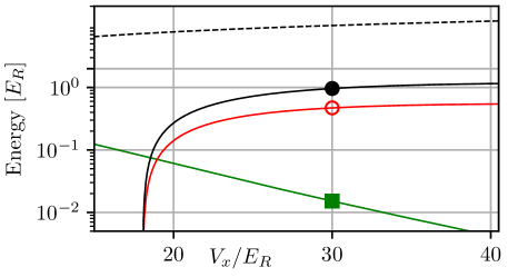
Figure 1: Figure shows the value of $f$ (black curve, marked with full circle), $\Delta_{sp}$ (black dashed line), and $U^{1111}$ (red solid line, marked with empty circle) assuming $U^{1120}=f/10$, $J^{1}$ (green curve, marked with a full square), for the classical optical potential $V_{\textrm{latt}}$ as the function of its height $V_{x}$ – see Eq. (7).

II.3 Standard optical lattice potential

The low-energy sector of a Hamiltonian [Eq. (1)] describing a particle in the lattice potential $V_{\textrm{latt}}(x)$ [Eq. (7)] for $V_{x}\gg E_{R}$ resembles a system with a series of almost-decoupled nearly-harmonic traps. Taking into account quartic terms in expansion of $\cos^{2}$ potential around its minima gives an approximate formula for $n$-th band energy:

$$E_{n}\approx\left(n+\frac{1}{2}\right)\sqrt{4V_{x}E_{R}}-E_{qu},\quad E_{qu}=\frac{6n^{2}+6n+3}{12}E_{R}.$$ (12)

The above expression is frequently used when truncated to just the first term $\sim\sqrt{V_{x}}.$ While it is often sufficient, we note that in $V_{x}\to\infty$ limit the quartic contribution $E_{qu}$ is non-vanishing. The $f$ defined in Eq. (11) for very large $V_{x}\gg E_{R}$, when all the hopping rates $J^{0},J^{1},J^{2}$ are exponentially suppressed is therefore:

$$f\approx 2E_{1}-E_{0}-E_{2}\to 1E_{R}$$ (13)

It is important to stress that the limit value in Eq. (13) is nonzero solely due to the quatric term in Eq.(12).

Specifically the $f$ is nonzero [see Fig. 1] for $V_{x}\gtrapprox 18E_{R}$ At around $V_{x}\approx 30E_{R}$, $f$ reaches $1E_{R}$. The maximum value of $f$ is attained near $V_{x}\approx 40E_{R}$ where $f\approx 1.4E_{R}$. Increasing the lattice height $V_{x}$ and therefore $f$ comes at the price of decrease of $J^{1}.$ For $V_{x}\approx 30E_{R}\,\,(40E_{R})$ we have $J^{1}\approx 0.015E_{R}\,\,(0.0042E_{R}).$

These $p$-band hopping rates are quite small. For a popular atom species used often in experiments, the ${}^{87}\textrm{Rb}$, typical parameters of lasers, the hopping frequency would be of the order of few tens of Hertz.

II.4 “Double-well” potential

By using two lasers one can create, by an AC-Stark shift a potential of the form (8). It has been used in countless theoretical and experimental works (just a few examples being (Anderlini et al., 2006; Stojanović et al., 2008; Lee et al., 2007; Sebby-Strabley et al., 2006; Anderlini et al., 2007)).

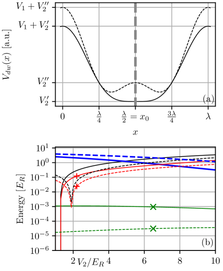
Figure 2: Figure shows the properties of the potential $V_{dw}$. Panel (a) parallels the discussion of the potential shape and symmetry in the main text; the vertical dashed gray line shows the symmetry axis. Solid line shows $V_{dw}$ for $V_{2}=V_{2}^{\prime}=V_{1}/4$. Dashed line shows $V_{2}=V_{2}^{\prime\prime}=V_{1}/2$ case. Panel (b) shows the value of $f$ (black curve), $\Delta_{sp}$ (blue, thick line), and $U^{1111}$ (red with a ’+’), $J^{1}$ (green with a ’$\times$’) assuming $U^{1120}=f/10$, for the two-well optical potential $V_{dw}$ as the function of $V_{2}$ with $V_{1}=10E_{R}$ (solid lines) or $V_{1}=20E_{R}$ (dashed lines). See Eq. (8).

The double-well potential $V_{dw}$ has a fundamental period twice larger than $V_{\textrm{latt}}(x)$, namely $a=\lambda$. When $\phi=0$ the potential is symmetric with respect to the center of the properly chosen unit cell $x_{0}$ [see Fig. 2(a)]. The Wannier functions of $s,p,d\ldots$ band are then alternately even an odd with respect to the $x_{0}.$ For $V_{2}\leq V_{1}/4$ the potential remains unimodal within the unit cell with minimum at $x_{0}$. At exactly $V_{1}=V_{2}/4$ at $\partial_{xx}V_{dw}(x_{\textrm{min}})=0$, and the potential around the minimum is well-approximated by a quartic potential [see Fig. 2(a)]. For larger $V_{2}$ there are two minima and the $s$ to $p$ band gap is significantly reduced.

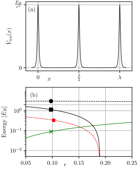
Figure 3: Figure shows the properties of the potential $V_{na}$. Panel (a) presents the shape and height of a potential $V_{na}$ parametrized by $\epsilon$. Panel (b) shows the value of $f$ (black curve with a square), $\Delta_{sp}$ (black dashed line with a circle), and $U^{1111}$ (red dashed line with a pentagon), $J^{1}$ (green with a cross) assuming $U^{1120}=f/10$, for the comb optical potential $V_{na}$ as the function dimensionless parameter $\epsilon$ – see Eq. (9).

The Fig. 2(b) shows the dependence of factor $f$ as a function of $V_{2}$ for fixed $V_{1}=10E_{R}$ (solid lines) and $V_{1}=20E_{R}$ (dashed lines). We see that for $V_{2}\approx V_{1}/4$ the factor $f$ is $0.35E_{R}$ for $V_{1}=10E_{R}$ and $f\approx 0.65E_{R}$ for $V_{2}=20E_{R}$ the values of $f$ reached are not larger than those achievable for the standard optical lattice ($f\leq 1.4E_{R})$. This is primarily due to twice larger period of the unit cell. As a result the increased anharmonicity due to the dominant quartic term is scaled down by factor 4, $E_{R}^{\prime}=\frac{h^{2}}{8ma^{2}}=\frac{E_{R}}{4},a=\lambda$. The value of $f$ can be increased by increasing both $V_{1}$ and $V_{2}$. For fixed $V_{2}=V_{1}/4$, in the limit of very large $V_{1},V_{2}$ the factor $f$ can be arbitrarily large (in contrast to the $V_{\textrm{latt}}$). The price to pay is the exponential decay of $J^{1}$, which for $V_{1}=10E_{R}$ is $O(10^{-3}E_{R})$ and for $V_{1}=20E_{R}$ is $O(10^{-5}\div 10^{-4}E_{R}).$ Increasing just $V_{2}$, while formally leading to the increase of $f$, actually leads to the degeneration of $p$ and $s$ band.

II.5 Comb potential

In this section we review in detail the construction of the comb potential (the presentation follows (Łącki et al., 2016)) with a particular focus on the parameters $\epsilon$ and $x_{0}$ which control the height and the position of the potential peak. The details of the construction are then referred to in discussion of $V_{\textrm{comb}}$ in the Subsection II.6.

The potential $V_{\textrm{{na}}}(x)$ as given by Eq. (9) transpires in the three level system (Łącki et al., 2016):

$$H_{\textrm{c}}=-\frac{\hbar^{2}}{2m_{a}}\partial_{x}^{2}+H_{\Lambda}(x),$$ (14)

where

$$H_{\Lambda}(x)=\hbar\left(\begin{array}[]{ccc}0&\Omega_{c}(x)/2&0\\ \Omega_{c}(x)/2&-\Delta-i\Gamma/2&\Omega_{p}/2\\ 0&\Omega_{p}/2&0\end{array}\right)$$ (15)

has been written in the atomic level basis $|g_{1}\rangle,|e\rangle,|g_{2}\rangle.$ The Rabi frequency $\Omega_{c}(x)$ is a standing wave,

$$\Omega_{c}(x)=\Omega_{c}\sin[k(x-x_{0})],$$ (16)

and $\Omega_{p}$ is $x$-independent,

$$\epsilon = \frac{\Omega_{p}}{\Omega_{c}}.$$ (17)

The position-dependent eigenstates of $H_{\Lambda}(x)$ include the dark state $|f_{1}(x)\rangle=-\cos\alpha(x)|g_{1}\rangle+\sin\alpha(x)|g_{2}\rangle$ with $\alpha(x)=\arctan[\Omega_{c}(x)/\Omega_{p}]$. It is an eigenstate to the zero energy for all $x$.

The Hamiltonian $H_{c}$ is well approximated by the following Hamiltonian (with $V_{na}$ given by Eq. 9):

$$H_{na} = -\frac{\hbar^{2}}{2m_{a}}\partial_{x}^{2}+V_{na}(x),$$ (18)

when it acts on wavefunctions of the form $\psi_{D}(x)=g(x)|f_{1}(x)\rangle$ of low energy $\langle\psi_{D}|H_{na}|\psi_{D}\rangle$ .

The potential $V_{na}$ has the form of sharp potential peaks [see 3(a)] of height $E_{R}/\epsilon^{2}$ and width $\sim\epsilon\lambda/2\pi$, located at $x=n\lambda/2+x_{0},n\in\mathbb{Z}.$

When $\epsilon\to 0$ the potential peaks can be replaced by $\frac{\pi}{2\epsilon}\sum_{n}\delta(x-x_{0}-n\lambda/2).$ In that limit, mean band energies converge to values characteristic for a box potential, $\bar{E}_{n}\approx n^{2}E_{R}.$ It may be shown that the bandwidths of each band $\Delta E_{n}\approx 4J^{n}\sim n^{2}\epsilon E_{R}$ [see (Łącki et al., 2016)].

The potential $V_{na}$ allows to reach similar values of $f$ as the standard optical lattice $V_{\textrm{latt}}$ ($f\approx 1.4E_{R}$ for $\epsilon=0.05$, and $f\approx 1E_{R}$ for $\epsilon=0.1$) [see Fig. 3(b)]. The anharmonicity of the mean band energies is $|2\bar{E}_{p}-\bar{E}_{s}-\bar{E}_{d}|\approx 2E_{R}$ but only for very small $\epsilon\approx 0$, the hopping $J^{0},J^{1},J^{2}$ is suppressed. Experiments conducted to this date operated with values of $\epsilon\geq 0.05$ (Wang et al., 2018; Tsui et al., 2019). Further reduction would necessitate using strong lasers creating the $\Omega_{c},\Omega_{p}$ which would couple the system beyond three levels included in (15). Use of atoms with trivial hyperfine structure would be a possible solution to te issues raised with first experiments. It should be also noted that the above $\Lambda$ system has not been so far experimentally realized with the bosonic species.

The values of hopping amplitude $J^{1}$ for $\epsilon\geq 0.05$ are actually order of magnitude larger than $J^{1}$ for $V_{\textrm{latt}}$ for same value of $f$ ($J^{1}\approx 0.09E_{R}$ for $\epsilon=0.1$, and for $\epsilon=0.05$ it is $J^{1}\approx 0.042E_{R}$). In contrast to $V_{\textrm{latt}}$ it is challenging to significantly reduce $J^{1}$ as the the potential barrier height $\sim\epsilon^{-2}$ increased with $\epsilon$ is partially compensated by its decreasing width $\sim\epsilon$. In the subwavelength comb the $s$ to $p$ and $s$ to $d$ band separations are almost $\epsilon$-independent and $\Delta_{sp}\approx 3E_{R},\Delta_{pd}\approx 5E_{R}$ .

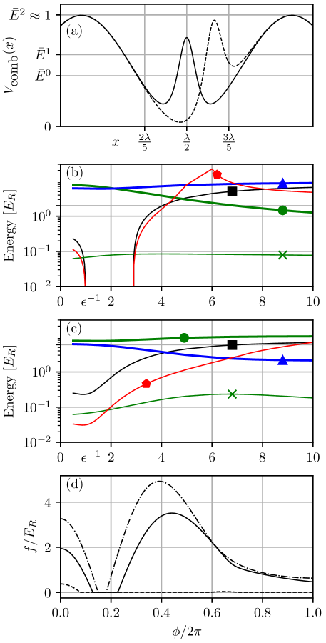
Figure 4: Properties of $V_{\textrm{comb}}$. Panel $(a)$ shows the potential shape, around the potential minimum for $V_{x}=20E_{R},\epsilon=0.25$ and $\phi=0$ (black solid line), $\phi=0.4/\pi$ (black dashed line). The levels $\bar{E}^{0}$,$\bar{E}^{1}$,$\bar{E}^{2}$ indicate first three band energies for $\phi=0$. Panels $(b)$ and $(c)$ show the value of $f$ (black curve with a square), $\Delta_{sp}$ (green, thick line with a filled circle), $\Delta_{pd}$ (blue, with a triangle pointing up), and $U^{1111}$ (red with a pentagon), $J^{1}$ (green with a cross) assuming $U^{1120}=f/10$, for the combined optical potential $V_{\textrm{comb}}$ (comb potential and classical $\sin^{2}$ potential) as the function of dimensionless parameter $\epsilon$ controlling the height of the comb potential with $V_{x}=20E_{R},\phi=0$ [panel $(b)$] or $V_{x}=20E_{R},\phi=0.4/2\pi$ [panel $(c)$]. See Eq. (8). Panel $(d)$ shows $f/E_{R}$ for $V_{x}=10,20,30E_{R}$ and $\epsilon^{-1}=4$ (dashed, solid, dash-dotted black line) as a function of a shift $\phi$ of subwavelength peak w.r.t to the potential minimum.

II.6 Classical potential together with the comb potential

Another possibility is opened by a combined potential that includes both a standard lattice potential $V_{\textrm{latt}}$ and the $V_{na}$ potential (parameter $\phi$ allows for shift of $V_{na}$ peak with respect to the minimum of $V_{\textrm{latt}}$) (Budich et al., 2017):

$$V_{\textrm{comb}}(x)=V_{\textrm{latt}}(x)+V_{na}(\epsilon,x-a\phi),\quad a=\lambda/2$$ (19)

The combined potential $V_{\textrm{comb}}(x)$ can be achieved when in Eq. (15) atoms in either of states $g_{1}$ and $g_{2}$ feel an additional, standard lattice potential due to AC-Stark shift, namely when the three-level Hamiltonian is of the form (Wang et al., 2018).

$$H_{\Lambda}(z)=\hbar\left(\begin{array}[]{ccc}V_{1}\sin^{2}(kx)&\Omega_{c}(x-a\phi)/2&0\\ \Omega_{c}(x-a\phi)/2&-\Delta-i\Gamma/2&\Omega_{p}/2\\ 0&\Omega_{p}/2&V_{1}\sin^{2}(kx)\end{array}\right).$$

The potential $V_{1}\sin^{2}(kx)$ is then simply added to $V_{na}(x-a\phi)$ resulting in the desired $V_{\textrm{comb}}(x)$.

In the pure $V_{\textrm{latt}}(x)$ potential the Wannier functions are alternately even an odd w.r.t to the center of the unit cell. A sharp potential in the middle of the cell, would primarily shift energies of each band, by a value $\int_{\mathbb{R}}V_{na}(x)|W^{\alpha}(x)|^{2}dx\approx\pi|W(0)|^{2}/(2\epsilon)$. The integral is maximal for the $s-$band Wannier functions, and decays for subsequent even Wannier functions. It is zero for odd bands, including the $p$-band. As the anharmonicity, for deep lattice is given by $f\approx 2\bar{E}^{1}-\bar{E}^{0}-\bar{E}^{2}>0$, adding the central $V_{na}$ peak should first lower the $f$ first towards zero. Only after that the $f$ can attain, large negative values.

Non-central placement of the $V_{na}(\epsilon,x)$ offers more flexibility in manipulating the $f\approx 2\bar{E}^{1}-\bar{E}^{0}-\bar{E}^{2}$ (see also (Budich et al., 2017)). For example, when the subwavelength peaks $V_{na}$ coincide with maxima of the $p$-band Wannier function of $V_{\textrm{latt}}(x)$ one can expect the mean $\bar{E}^{1}$ to increase strongly in contrast to $\bar{E}^{0}$ and $\bar{E}^{2}$. As a result the band anharmonicity should be increased to large positive values.

In Fig. 4(a) shows the parameters describing the properties of the $V_{\textrm{comb}}$ for $\phi=0$ and for $\phi=0.4/\pi$. In the latter case $V_{na}(x-a\phi)$ nearly coincides with maximum of the $p$-band Wannier function.

When $\phi=0$ it is evident that the values of $f$ that easily achieve value of $f=2E_{R}$ (for $\epsilon\approx 0.25)$ before, for even smaller $\epsilon,$ the central peak given by $V_{na}$ cuts the potential well into two almost disconnected parts, with tiny $\Delta_{sp}$. For $\phi=0$ we focus on $\epsilon\approx 0.25$ when the $\bar{E}^{1}$ is similar to the $V_{na}$ peak height, the Wannier function of the $p$ band is not strongly affected by the potential peak and $\Delta_{sp}$ remains sizable.

For small $\epsilon^{-1}$ the potential $V_{\textrm{comb}}$ can resemble the potential $V_{dw}.$ The crucial difference is that its period remains $a=\lambda/2$ in contrast to period $\lambda$ of $V_{dw}$. This allows to maintain much higher hopping rate in $V_{\textrm{comb}.}$

When $\phi=0.4/\pi$ the values of $f$ that are reached are similar, with important difference: the value of $f=2\bar{E}^{1}-\bar{E}^{0}-\bar{E}^{2}$ for $\epsilon^{-1}\to 0$ does not change the sign as $\epsilon^{-1}$ is increased. This means that in contrast to $\phi=0$, also for $\epsilon^{-1}\leq 3$ the $f$ is nonzero. This is important for practical applications as the spontaneous emission losses quickly grow with $\epsilon^{-1}$ (see (Łącki et al., 2016; Wang et al., 2018)).

For all considered $\phi$ the hopping rate $J^{1}\approx 0.1\div 0.15E_{R}$. It is half of the order of magnitude larger than for $V_{\textrm{latt}}$of the same potential height. This is simply due to the fact that putting extra potential $V_{na}$ in the potential well makes it effectively shallower. In contrast to using a standard optical lattice $V_{\textrm{latt}}$ working with the value of $f\approx 1-2E_{R}$ requires $V_{x}=15\div 20E_{R}$ while for $V_{\textrm{latt}}$ the $f\approx 1-1.4E_{R}$ is reached for deep lattices of $V_{x}=30\div 40E_{R}$ with $J^{1}$ hopping rate significantly reduced. At such value of $\epsilon$ the combined potential retains workable features of the $V_{\textrm{latt}}$ such as sizable $\Delta_{sp}\approx 3.8E_{R}$.

III Collisional stability of p-band condensate

Figure 5: Mean losses from the $p$-band population of an interacting system for the four considered potentials, in a system of length $L=6$ populated with $\rho L=7`$ particles. The exact parameters are given by Eqs. (20)-(24).

In this section we numerically study the stability of the $p$-band gas in the potentials from the previous Section II. To this end we consider a small, strongly interacting system consisting of $L=6$ sites described by Hamiltonian $H_{\textrm{MBH}}$ in Eq. (2) under periodic boundary conditions, restricted to lowest three bands, $\alpha_{\textrm{max}}=3.$

1. Potential $V_{\textrm{latt}}$ of height $V_{x}=30E_{R}$ with $f\approx 1E_{R}$ and:

   $$(J^{0},J^{1},u,u^{\prime})\approx(-0.00046E_{R},0.015E_{R},0.698,4.89),$$ (20)

2. Potential $V_{na}$ for $\epsilon=0.1$ with $f\approx 1.11E_{R}$ and:

   $$(J^{0},J^{1},u,u^{\prime})\approx(-0.022E_{R},0.091E_{R},0.985,3.05),$$ (21)

3. Potential $V_{\textrm{comb}}$ of $V_{2}=20E_{R}$, $\epsilon=0.25,\phi=0$ with $f\approx 1.94E_{R}$ and:

   $$(J^{0},J^{1},u,u^{\prime})\approx(-0.024E_{R},0.084E_{R},0.933,9.02),$$ (22)

4. Potential $V_{\textrm{comb}}$ of $V_{2}=20E_{R}$, $\epsilon=0.25,\phi=0.4/2\pi$ with $f\approx 3.38E_{R}$ and:

   $$(J^{0},J^{1},u,u^{\prime})\approx(-0.00074E_{R},0.11E_{R},0.445,5.88),$$ (23)

5. Potential $V_{dw}$ of $V_{1}=20E_{R},V_{2}=4E_{R}$ with $f\approx 0.65E_{R}$ and:

   $$(J^{0}\!,J^{1}\!,u,u^{\prime})\approx(-1.16\!\times\!10^{-6}E_{R},2.5\!\times\!10^{-5}E_{R},0.802,4.00).$$ (24)

Initially the quantum state of the gas of $N_{p}=\rho L$ particles is an eigenstate $\psi_{0}$ of the Hamiltonian $H_{\textrm{MBH}}$, Eq. (2) with no interactions, $g=0$. The chosen initial state is the least energy eigenstate where all the particles populate the $p$-band – it is a product of Bloch functions with quasimomentum $q=q_{*}$ minimizing $E^{1}(q)$.

The subsequent evolution $\psi(t)=\exp(-iH_{\textrm{MBH}}t/\hbar)\psi_{0}$ is governed by full $H_{\textrm{MBH}}$ truncated to lowest three bands, $\alpha<\alpha_{\textrm{max}}=3$. The population of the $p$-band is given by

$$N_{p}(t)=\langle\psi(t)|\hat{n}_{p}|\psi(t)\rangle$$

Initially, $N_{p}(t=0)=\rho L$. For $t>0$ the population $N_{p}(t)$ drops due to interaction-driven coupling to other bands. The temporal dependence shows some long-term oscillatory behavior that is attributed to the finiteness of the system and that of the Hilbert space. To mitigate these effects, we consider a long-time average $L_{p}=\overline{N_{p}(t)}.$

Let us discuss the dependence of $N_{p}(t)$ and $L_{p}$ on the interaction strength $g$, that can be altered by means of a Feshbach resonance (Chin et al., 2010).

The value of $\xi=J^{1}/U^{1111}$ parameter together with $\rho$ indicate the position in the phase diagram of the BH model. The absolute value of $J^{1}$ [Eqs. (20)-(24)] is however smaller by $V_{\textrm{latt.}}$ of $V_{dw}$ by order of magnitude or more than $V_{na}$ or $V_{\textrm{comb.}}$. To ensure that all four cases correspond to the same quantum phase – superfluid state, we fix the system density to $\rho=7/6>1$. As a result all the four systems have essentially the same probability for double occupation of the lattice site.

Under such assumptions the relative loss defined as $\delta=(\rho L-L_{p})/\rho L$ measures the depletion of the $p$-band. As revealed by a numerical simulation, for as long as $U^{1111}\ll f$ the losses $\delta$ for potentials $V_{\textrm{latt}},V_{na},V_{\textrm{comb}},V_{dw}$ scale as $\delta=A(U^{1111}/E_{R})^{\alpha}.$ Fitting the numerical data show in Fig. 5 we find that for $V_{\textrm{latt}}$ we have $A=0.13900\pm 0.00028,\alpha=1.83090\pm 0.00039$; for $V_{na}$ we have $A=0.28983\pm 0.00042,\alpha=1.92133\pm 0.00028$; for $V_{\textrm{comb}}$ we have $A=0.093\pm 9.0\cdot 10^{-5},\alpha=1.9610\pm 0.0050$; for $V_{dw}$ we have $A=0.94703\pm 0.00054,\alpha=1.97562\pm 0.00011$. The fittings, as evident from Fig. 5 differ mainly by the prefactor, with losses for the $V_{\textrm{comb}}$ being smaller with respect to the $V_{\textrm{latt}}$ by approximately $30\textrm{\%}$ for same value of $U^{1111}$. Together with order of magnitude larger $J^{1}$ potential $V_{\textrm{comb}}$ provides a compelling way to realize a weakly interacting $p$-band superfluid.

When the offset of the subwavelength peak is introduced, for $\phi=0.4/2\pi$ which maximizes the $f$-factor. The loss rate scaling is given by $A=0.0863\pm 0.0002,\alpha=1.96956\pm 0.00043$. This offers only marginal improvement over $\phi=0$ case. As can be seen in Eqs. (22) and (23), while the factor $f$ is increased from $1.94E_{R}$ to $3.38E_{R}$ the ratio of $U^{1111}/U^{1120}$ is decreased from 9.02 down to 5.88. This means that for same $U^{1111}$ the value of $U^{1120}$ is actually larger in the $\phi\neq 0$ case. This consumes all benefits from increasing the $f$ as $f/U^{1102}$ is essentially the same in both cases.

IV Resonant coupling of $S-$band to $P-$band

IV.1 Synthetic ladder

Figure 6: Mean losses from $s-p$ band, noninteracting ladder system measured as $\bar{N}_{d}$ population as a function of $T_{R}$ – Rabi frequency oscillation between $s$ and $p$ band (see text). Black triangles, red crosses, blue circles, green stars show losses for $V_{\textrm{latt}},V_{na},V_{dw},V_{\textrm{comb}}$ lattices, for ($V_{x}=30E_{R},$ $\epsilon=0.1,$ $V_{1}=20E_{R},\phi=0$ $\textrm{ and }V_{2}=4E_{R},$ $V_{1}=20E_{R}$ and $\epsilon=0.25$ respectively). The cyan $V_{\textrm{comb}}^{\prime}$ data series for configuration of $V_{\textrm{comb}}$ but with $\phi=0.4/2\pi$.

Coupling of the $s$ and $p$ bands can be achieved by a periodic modulation of the system with the frequency $\omega=\bar{E}^{1}-\bar{E}^{0}$ (see (Gemelke et al., 2005; Sowiński, 2012; Łącki and Zakrzewski, 2013; Cabrera-Gutiérrez et al., 2019)). The other bands are off-resonant if $\omega=\bar{E}^{1}-\bar{E}^{2}\neq 0$ and in first approximation they can be neglected. We will study the degree to which neglecting other bands is possible for different potentials considered in this work.

The simplest coupling the bands $s$ and $p$ is by periodic modulation of the position of the lattice:

$$V(x,t)=V(x-A\sin\omega t).$$

The potential oscillation implies a co-movement of the instantaneous Wannier functions:

$${\cal W}_{n}^{\alpha}(x,t) = {\cal W}_{n}^{\alpha}(x-A\sin\omega t)$$

For fixed $t$ the Hamiltonian (1), in the basis set by ${\cal W}_{i}^{\alpha}(x,t)$, will take the form of $H_{\textrm{MBH}}$ with time-independent coefficients. Nevertheless, correctly derived time-evolution equation of motion, has to take into the account the time-dependence of the basis. The resulting Time dependent Schrödinger equation is of the form (Łącki and Zakrzewski, 2013; Pichler et al., 2013):

$$\partial_{t}\psi = H_{\textrm{MBH}}\psi-\sum_{i}\sum_{\alpha,\beta}[{\cal T}_{ii}^{\alpha\beta}A\omega\cos\omega t](a_{i}^{\alpha})^{\dagger}a_{i}^{\beta}\psi.$$ (25)

The extra terms proportional to $T_{nm}^{\alpha\beta}$ do not couple within the same band as $\forall m,n:{\cal T}_{nm}^{\alpha\alpha}=0$. If the potential is symmetric with respect to the middle of the unit cell, the coefficients ${\cal T}_{ii}^{\alpha\beta}=0,\alpha+\beta\equiv 0\,(\!\!\!\!\mod 2),$ and they couple just bands of opposite parity, for example $s$ and $p$ band, but also e.g. $p$ to the $d$ band.

A 1D optical system, where population of bands other than $s$ and $p$ is precluded can be seen as a two leg ladder system [see Fig. 6(a)]. This shares many features with the synthetic dimension construction where in lieu of bands, different hyperfine states are used (Celi et al., 2014). In particular, two sites at the ends of same ladder step, are physically in the same place, possibly allowing for strong interaction. The hoppings along the each of the lattice legs is governed by $J^{0}$ and $J^{1}$ respectively, possibly allowing to implement complex ladder systems such as (Li et al., 2011).

With no interaction, such an effective single particle system decomposes into fixed quasimomentum sectors:

$$i\hbar\partial_{t}\left(\begin{array}[]{c}\psi_{k}^{0}\\ \psi_{k}^{1}\end{array}\right) \!\!=H_{\textrm{ladd}} \left(\begin{array}[]{c}\psi_{k}^{0}\\ \psi_{k}^{1}\end{array}\right),$$ (30)

where:

$$H_{\textrm{ladd}}=\left(\begin{array}[]{cc}E^{0}(k)&iT^{01}A\omega\cos(\omega t)\\ -iT^{01}A\omega\cos(\omega t)&E^{1}(k)\end{array}\right).$$ (31)

By transforming to a rotating frame $(\psi_{k}^{0}e^{i\delta_{0}t},\psi_{k}^{1}e^{i\delta_{1}t})$ and using the RWA, the equation of motion becomes time-independent, when $\delta_{2}-\delta_{1}=\omega$:

$$i\hbar\partial_{t}\left(\begin{array}[]{c}\psi_{k}^{0}\\ \psi_{k}^{1}\end{array}\right) \!\!=\!\! H_{\textrm{ladd},\textrm{RWA}}\!\!\left(\begin{array}[]{c}\psi_{k}^{0}\\ \psi_{k}^{1}\end{array}\right),\,\,\,\Omega=T^{01}A\omega,$$ (36)

where

$$H_{\textrm{ladd},\textrm{RWA}}=\left(\begin{array}[]{cc}E^{0}(k)-\hbar\delta_{0}&\Omega\\ \Omega&E^{1}(k)-\hbar\delta_{1}\end{array}\right).$$ (37)

When $\delta_{i}\approx E^{i}(k)$, the Rabi oscillations frequency is $\Omega=T^{01}A\omega$. For $\Omega$ dominating the bandwidths $\Delta E^{i}$ this behavior is $k$-independent and Eq. (31) can be written as:

$$H_{L} = -J^{0}\sum_{n=1}^{L}(a_{n}^{0})^{\dagger}a_{n+1}^{0}-J^{1}\sum_{n=1}^{L}(a_{n}^{1})^{\dagger}a_{n+1}^{1}+H.c.$$ (39)

$$+i{\cal T}_{n}^{01}A\omega(a_{n}^{0})^{\dagger}a_{n}^{1}\cos\omega t+H.c.+H_{\textrm{int.}},$$

where

$$H_{L,\textrm{int}}=\sum_{n}\frac{U_{nnnn}^{\alpha\beta\gamma\delta}}{2}\sum_{\alpha,\beta,\gamma,\delta=0,1}(a_{i}^{\alpha})^{\dagger}(a_{i}^{\beta})^{\dagger}a_{i}^{\gamma}a_{i}^{\delta}.$$ (40)

When coupling to other bands beyond $s$ and $p$ cannot be neglected, system fails to be modeled by a two-leg ladder. This deviation from the ladder system is again measured by mean occupation of $d$ and higher bands, $\delta=\bar{N}_{\geq d}/N_{\textrm{tot}}$. Depletion is possible also by means of the interaction.

Figure 7: Depletion of the $s,p$ band by as a function of $\bar{U}=(U^{0000}+U^{1111})/2$ for such an oscillation amplitude that corresponds to $T_{R}E_{R}/\hbar=0.02$ in Fig. 6 At $\bar{U}=0$ the depletion is finite and solely due to off-resonant coupling of $s,p$ band to higher $d$ band. Increase of the interaction results in further depletion of $s,p$ band. The legend identifies the four potential discussed in the main text. The $V_{\textrm{comb}}$ potential is characterized by losses smaller for large interaction approximately by an order of magnitude, despite much larger hopping values.

IV.2 Realization in different potentials

In this section we compare the implementations of Eq. (39) where the $s$ and $p$ bands are taken from the four discussed potentials. Specifically, the “perfect ladder” system is Eq. (25) truncated to the $s,p$ bands. This leads to the desired Eq. (39). The closedness of such a system is compared to the model that also includes the $d$ band, which is the most relevant band to consider in the study of couplings to other bands. Out of all bands beyond $s,p$ the $\omega=\bar{E}^{1}-\bar{E}^{0}$, for the class of potentials we consider, is closest to $\bar{E}^{2}-\bar{E}^{1}.$

To meaningfully compare the four potentials we pick the same realizations in the Section III. In addition to parameter values given in Eqs. (20)-(24), we have that for $V_{\textrm{latt}},$$V_{na},$$V_{\textrm{comb}},$$V_{dw}$ the ${\cal T}^{01}\approx 1.57E_{R},0.85E_{R},0.77E_{R},0.86E_{R}$ respectively. For the $V_{\textrm{comb}}$ potential for $\phi=0.4/2\pi$ we have $T^{01}\approx 1.36E_{R}.$ It should be noted that in the latter case, due to lack of symmetry of the unit cell, also $T^{02}\approx 0.49E_{R}.$

We opt to compare the ladder depletion in the four potentials when all in all four cases the Rabi oscillation period $T_{R}$ takes the same value. Ordinarily $T_{R}=2\pi/\Omega$ with $\Omega=|T^{01}A\omega|$. When coupling to the $d$ band is included and becomes significant, the system does not undergo pure Rabi oscillation. More complicated oscillation pattern emerges. We define $T_{R}$ for each amplitude of modulation by fitting the $A+B\sin(t/T_{R})$ to the temporal dependence of $N_{s}(t)$.

First we consider a non-interacting ladder system of total length $L=40$. We initialize the evolution with a quasi-momentum $k=0$ state $\psi_{0}$ in the $s$-band, By fixing initial $k$ allows consider $\Omega$ smaller than the bandwidth and still observe model Rabi oscillations, by setting $\omega=E^{1}(k=0)-E^{0}(k=0)$. As pictured in Fig. 6, the losses measured by $\bar{N}_{d}$, in the limit of small $T_{R}$ scale as $\bar{N}_{d}=A(T_{R})^{\alpha}$. For the four potentials we find that : $\bar{N}_{d,\textrm{latt}}=(0.278\pm 0.026)T_{R}^{1.909\pm 0.020}$,$\bar{N}_{d,na}=(0.123\pm 0.013)T_{R}^{1.899\pm 0.022}$,$\bar{N}_{d,\textrm{comb}}=(0.0501\pm 0.0053)T_{R}^{1.909\pm 0.022}$,$\bar{N}_{d,dw}=(2.94\pm 0.10)T_{R}^{1.9564\pm 0.0071}$. For the alternative implementation of $V_{\textrm{comb}}$ with $\phi=0.4/2\pi$ we get $\bar{N}_{d,\textrm{comb}}^{\prime}=(0.055\pm 0.0031)T_{R}^{1.974\pm 0.011}$. This scaling applies when $\bar{N}_{d}\ll 1$, In all cases we find that $\bar{N}_{d,\textrm{comb}},$ are approximately an order of magnitude smaller than $\bar{N}_{d,\textrm{latt}},$ with $\bar{N}_{d,na},$ being in between. The losses for the double-well are order of magnitude larger than for the remaining systems. This is because of the lowest value of $f\approx 0.65E_{R}$ out of the four samples. The potential $V_{\textrm{comb}}$ with $\phi=0.4/2\pi$ again offers same stablity as the $\phi=0$. Nevertheless it features a strongly suppressed $J^{0}$ hopping along one of the lattice “legs” [as implied by Eq. (22) and Eq. (23)].

If the modulated system is also interacting an interesting interplay of shaking and interaction may occur. To simulate such a case we consider the same four potentials, modulated with a modulation amplitude $A$ such that the noninteracting Rabi oscillation period $T_{R}=0.02\hbar/E_{R}$. The length of the lattice is $L=6$ with total $\rho L=7$ particles.

The Fig. 7 shows the dependence of the $\bar{N}_{d}$ on the mean interaction strength $\bar{U}=(U^{0000}+U^{1111})/2$ (see also (20)-(24)). The interaction strength would be tuned with use of the Feshbach resonance, thus scaling both $U^{1111},U^{0000}$ by a common factor. For $\bar{U}=0$ the results from Fig. 7 are reproduced. For increasing $\bar{U}>0$ for each of the four potentials the interaction causes the additional losses on top of the modulation losses. It is evident that the losses for the $V_{\textrm{comb}}$ potential grow slowest with the $\bar{U}$ [here again losses for $\phi=0$ are essentially the same as for $\phi=0.4/2\pi$]. This is due to the combination of factors: first it allows to reach high anharmonic band placement (large value of $f\approx 2E_{R})$, second as evident from Fig. 4 the value of $|U^{1102}/\bar{U}|$ is relatively small compared to other potentials 0.17,0.32,0.11,0.23 for $V_{\textrm{latt}},V_{na},V_{\textrm{comb}},V_{dw}$ (for $V_{\textrm{comb}}$ for $\phi=0.4/2\pi$ we have $|U^{1102}/\bar{U}|\approx 0.105$ ). This means that if $\bar{U}$ is fixed to a given value, then the terms responsible for interaction-driven losses come with a smaller prefactor than in the other potentials. This advantage together with largest value of $f$ (which affects also modulation) allows to observe order of magnitude smaller depletion of the $s,p$ band system. This also explains the difference in stability for $\bar{U}\neq 0$.

V conclusions and outlooks

The subwavelegth comb potential makes it possible to implement potentials that break the constraints implied by the diffraction limit put on constructions based on the AC-Stark effects. We have constructed lattice potentials with anharmonic potential wells, that can be realistically implemented in laboratory. The anharmonicity enhances the collisional stability of the $p$-band gas. Moreover, the $s$ and $p$ bands of the lattice can be resonantly coupled by modulation, and the resulting couplings from $s,p$ bands to other bands can be sufficiently off-resonant to neglect them for even stronger coupling strength than the standard lattice. The latter was presented by implementing a synthetic dimension $s-p$ band ladder.

Another important feature of the constructed potentials is the ability to preserve large value of the hopping rate. They offer controllable work with the $p$ band in the regime of large hopping amplitude.

The remaining open question is the applicability of the construction for the interacting bosonic systems. A fundamental problem is description of interaction-driven depletion of dark states, and a choice of a proper atom species that would allow the $\Lambda$ system construction in for an collisionally interacting ultracold atom gas.