Long-range fluctuation–induced forces in driven electrolytes

Abstract

We study the stochastic dynamics of an electrolyte driven by a uniform external electric field and show that it exhibits generic scale invariance despite the presence of Debye screening. The resulting long-range correlations give rise to a Casimir-like fluctuation–induced force between neutral boundaries that confine the ions; this force is controlled by the external electric field, and it can be both attractive and repulsive with similar boundary conditions, unlike other long-range fluctuation–induced forces. This work highlights the importance of nonequilibrium correlations in electrolytes and shows how they can be used to tune interactions between uncharged biological or synthetic structures at large separations.

Fluctuation–induced forces (FIFs) can arise in a wide range of systems where external objects modify the spectrum of the fluctuations in a correlated medium [1, 2]. Such forces only act at short distances when the confined fluctuations have a finite correlation length, for instance the Debye screening length in electrolytes [3, 4]; scale-free correlations, however, can give rise to long-ranged FIFs with universal properties [5], e.g., in the case of Casimir attraction between metallic plates in vacuum [6] and forces arising from critical fluctuations in thermal equilibrium [7, 8]. The extent to which critical Casimir forces can be controlled have especially been investigated in recent years due to their practicality in colloidal systems [9]. Out of thermal equilibrium, long-range correlations are common as they arise, e.g., from the interplay between the conservation laws and a mismatch between fluctuations and dissipation [10, 11, 12]. The ensuing FIFs have been studied in a variety of settings such as nonuniform temperature profiles [13], nonequilibrium diffusive dynamics [14], temperature quenches [15, 16], active systems [17], and Brownian and driven charged particles [18, 19].

Confined electrolytes are highly structured fluids [20] that are ubiquitous in various areas of nanotechnology [21, 22] and biology [23, 24], for instance in biological or synthetic nanopores (see Fig. 1). Recently, there have been experimental observations of force generation in charged solutions which deviate considerably from mean-field predictions [25, 26]. It is therefore desirable to understand the generic mechanisms by which correlations in these systems may give rise to fluctuation–induced interactions.

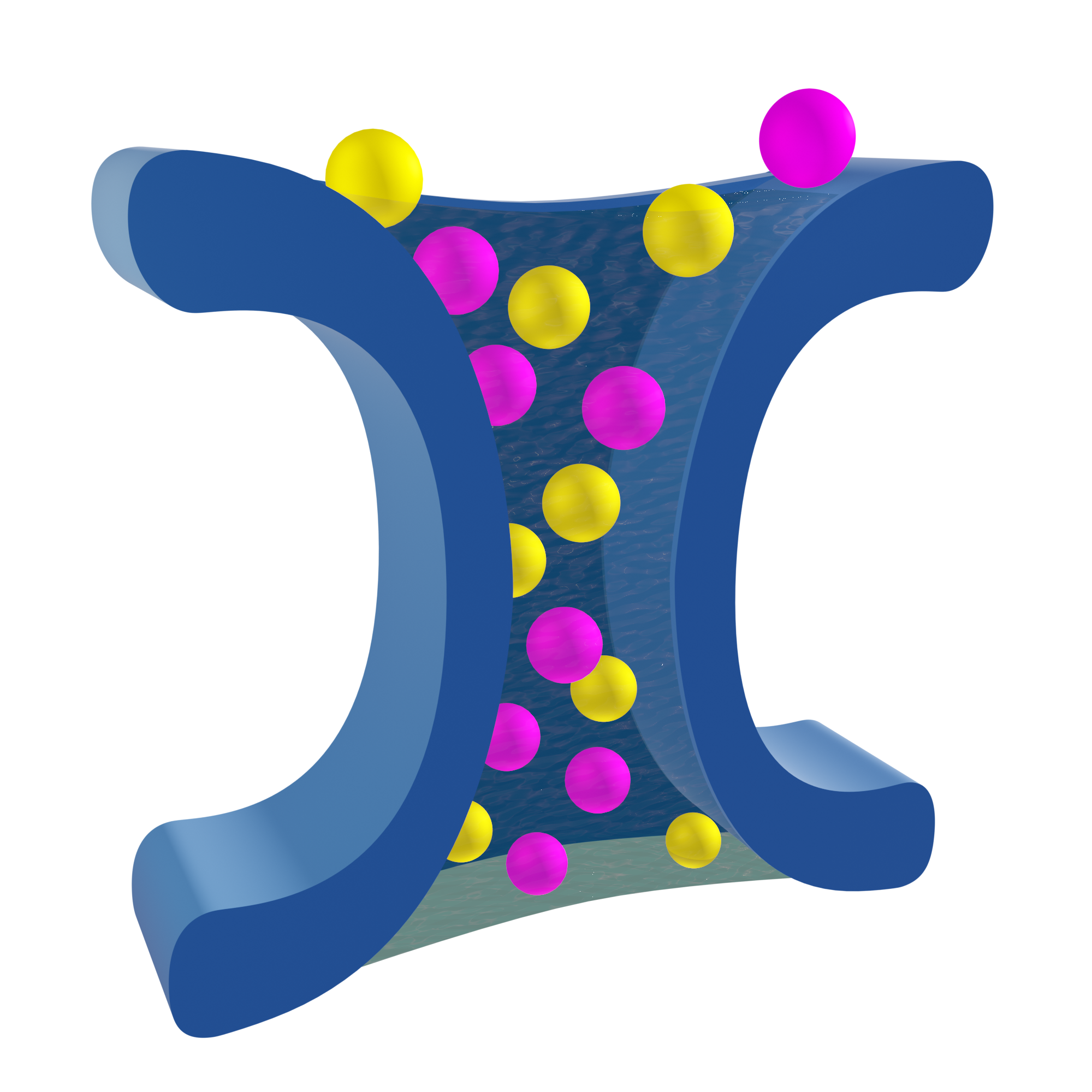
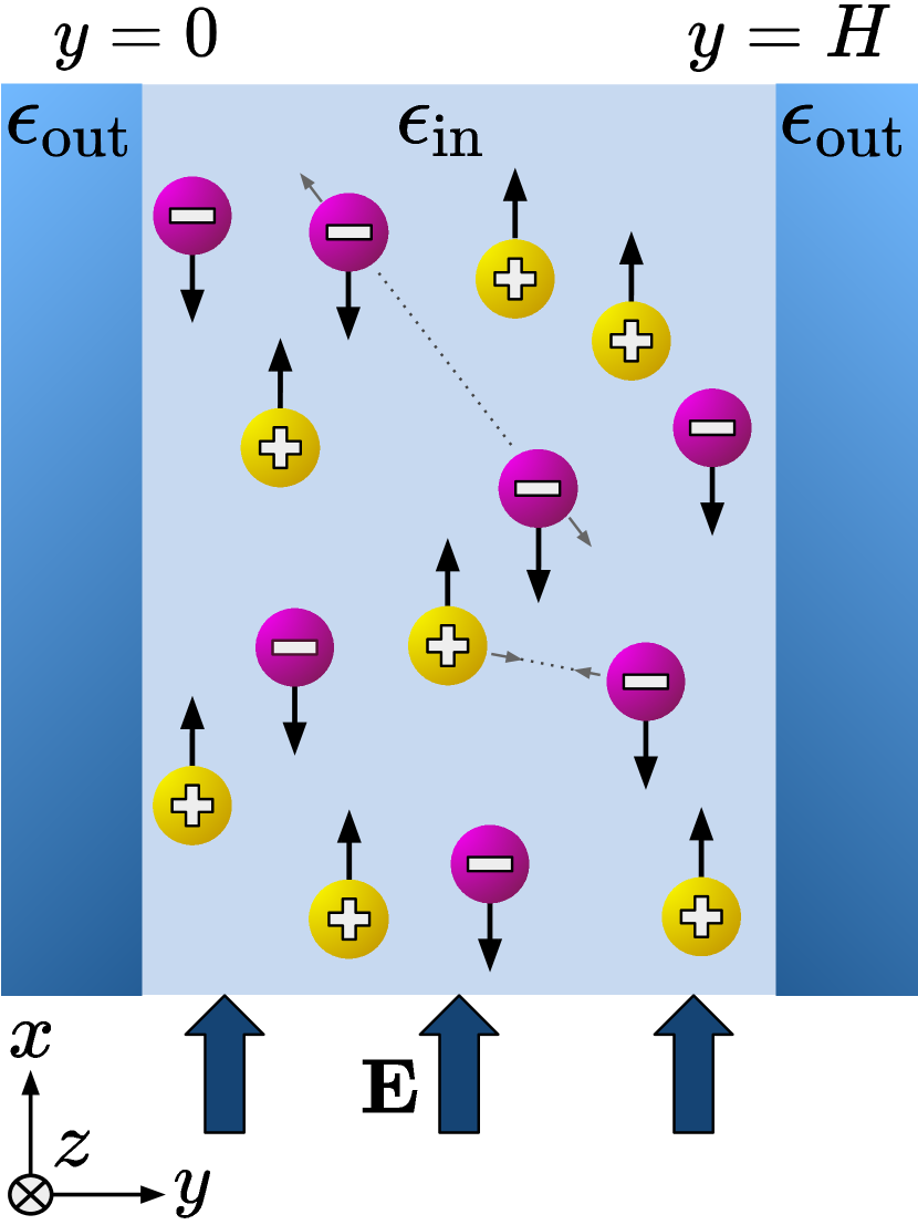
Figure 1: Schematics of an ion channel (left) and the generic setup of a driven electrolyte in flat geometry studied here (right). The external electric field $\bm{E}=E\hat{\bm{e}}_{x}$ drives the positive and negative charges in opposite directions (black arrows) and, in addition, the charges exert electrostatic forces on each other (gray arrows). The system is open along the $x$ and $z$ axes, and it is confined by neutral plates (with similar boundary conditions) in the $y$ direction.

It is well known that in thermal equilibrium, the correlations in an electrolyte are exponentially screened beyond the Debye length [27]. Here, we examine the long-distance behavior of a strong electrolyte when it is driven out of equilibrium by an external electric field, and we show that the anisotropy introduced by the electric field gives rise to power-law correlations and generically scale invariant dynamics [28, 29]. Such scale-free correlations have considerable implications on the dynamics of external boundaries that enclose the electrolyte. Using the Maxwell stress tensor, we calculate the FIF that results from confining the electrolyte driven by the external field $\bm{E}=E\hat{\bm{e}}_{x}$ parallel to neutral flat boundaries (see Fig. 1); we find that in $d$ spatial dimensions, the normal force per unit area of the plates is given by

$$\frac{F}{S}=-\frac{k_{\rm B}T}{H^{d}}\,\mathcal{E}^{4}\,\mathcal{A}(\mathcal{E},\lambda)=-\frac{\big{(}\frac{\epsilon_{\rm in}}{2S_{d}}E^{2}\big{)}^{2}}{k_{\rm B}TC_{0}}\cdot\frac{\mathcal{A}(\mathcal{E},\lambda)}{C_{0}H^{d}},$$ (1)

where $H$ is the separation between the plates. This force depends on the dimensionless parameter $\mathcal{E}$, which represents the ratio between the electric field (Maxwell) stress and the osmotic pressure of the electrolyte, and on the dielectric contrast $\lambda$ that are defined as follows

$$\mathcal{E}=\left[\frac{\frac{\epsilon_{\rm in}}{2S_{d}}E^{2}}{k_{\rm B}TC_{0}}\right]^{1/2},\qquad\text{and}\qquad\lambda=\frac{\epsilon_{\rm in}-\epsilon_{\rm out}}{\epsilon_{\rm in}+\epsilon_{\rm out}}.$$ (2)

In these relations, $\epsilon_{\rm in}$ and $\epsilon_{\rm out}$ are the permittivities of the electrolyte and the boundary material, respectively, $C_{0}$ is the mean concentration (of each charge) in the electrolyte, and $S_{d}=\frac{2\pi^{d/2}}{\Gamma(d/2)}$ is the area of the $d$-dimensional unit sphere. The dimensionless amplitude $\mathcal{A}$ is independent of the applied field for $\mathcal{E}\ll 1$, implying that the FIF scales as $\sim E^{4}$ for relatively weak electric fields; for $\mathcal{E}\gg 1$, on the other hand, one has $\mathcal{A}\sim 1/\mathcal{E}^{2}$, and therefore for large applied electric fields the force scales as $\sim E^{2}$ (see Table. 1 and Fig. 2). Intriguingly, the amplitude $\mathcal{A}$ varies non-monotonically with $\mathcal{E}$ (in addition to $\lambda$), and it can also change sign (see Fig. 2). The sign change indicates that the resulting FIF can be tuned to be both repulsive and attractive in the same setup with symmetric boundary conditions. It is worth noting that the force studied here is purely due to fluctuation effects and a change in the sign of this generic long-range FIF is a unique feature that distinguishes our results from, e.g., modifications of critical Casimir forces on introducing additional surface or bulk features that contribute to the force [31, 32, 33, 34, 35].

Stochastic Density Equations— We consider a strong simple electrolyte which consists of an equal number of cations and anions with charges $\pm Q$ and with equal mobilities $\mu_{+}=\mu_{-}=\mu$. The individual cations and anions, labeled by $a$, move under the combined influence of the external electric field ($\bm{E}$), the electrostatic field of other ions ($-\nabla\phi$), and Brownian motion [36] due to thermal noise ($\bm{\eta}_{a}^{\pm}$). In the overdamped regime, the trajectory $\bm{r}^{\pm}_{a}(t)$ of a cation or anion is governed by the Langevin dynamics $\dot{\bm{r}}_{a}^{\pm}(t)=\mu\left(\pm Q\right)\left[-\nabla\phi\big{(}\bm{r}_{a}^{\pm}(t)\big{)}+\bm{E}\right]+\sqrt{2D}\,\bm{\eta}_{a}^{\pm}(t)$ [37, 38]. The thermal noises $\bm{\eta}_{a}^{\pm}$ are independent Gaussian white noises characterized by $\langle\eta_{ai}^{+}(t)\eta_{bj}^{+}(t^{\prime})\rangle=\langle\eta_{ai}^{-}(t)\eta_{bj}^{-}(t^{\prime})\rangle=\delta_{ab}\,\delta_{ij}\,\delta(t-t^{\prime})$ and zero mean ($a$ and $b$ are particle indices and $i$ and $j$ represent vector components). At this microscopic level, the fluctuation–dissipation relation connects the noise strength $D$ to the mobility $\mu$ through the Einstein relation $\mu=\beta D$, where $\beta=1/(k_{\rm B}T)$ is the inverse temperature. Note that we neglect the hydrodynamic effects of the solvent throughout this work .

Using the instantaneous number density of each type of charge, which is defined as $C^{\pm}(\bm{r},t)=\sum_{a}\delta^{d}\left(\bm{r}-\bm{r}_{a}^{\pm}(t)\right),$ one can express the electrostatic Poisson equation in Gaussian units as $-\nabla^{2}\phi=\frac{S_{d}Q}{\epsilon_{\rm in}}(C^{+}-C^{-}).$ The Dean–Kawasaki approach [40, 41, 42] then gives the exact dynamics of $C^{\pm}$ as continuity equations, namely $\partial_{t}C^{\pm}+\nabla\cdot\bm{J}^{\pm}=0$, where the stochastic currents of the charges are given by $\bm{J}^{\pm}=-D\nabla C^{\pm}\pm\mu C^{\pm}Q\left(-\nabla\phi+\bm{E}\right)-\sqrt{2DC^{\pm}}\,\bm{\eta}^{\pm}.$ Here, $\bm{\eta}^{\pm}$ are uncorrelated Gaussian noise fields with zero averages and $\langle\eta_{i}^{\pm}(\bm{r},t)\eta_{j}^{\pm}(\bm{r}^{\prime},t^{\prime})\rangle=\delta_{ij}\delta^{d}(\bm{r}-\bm{r}^{\prime})\delta(t-t^{\prime})$.

The Dean–Kawasaki equations for $C^{\pm}$ are analytically intractable due to the nonlinear terms and the multiplicative noise. To avoid these difficulties, we consider the dynamics of the density and charge fluctuations around a state with uniform distribution of the particles, which allows us to linearize the dynamics. This simplification remains valid for a dense population of soft particles [43] and has been used, e.g., to study the conductivity of strong electrolytes [38], fluctuations of ionic currents across nanopores [37, 44], and the universal correlations in driven binary mixtures [45]. We have also examined the scaling behavior of the nonlinear terms which reveals that these nonlinearities are irrelevant at the macroscopic level (see Ref.  for details). We therefore write the density of each type of charge as $C^{\pm}=C_{0}+\delta C^{\pm}$ and assume the density fluctuations $\delta C^{\pm}$ are small compared to the background $C_{0}$, i.e., $\delta C^{\pm}\ll C_{0}$. Introducing the number fluctuations $c(\bm{r},t)=\delta C^{+}+\delta C^{-}$ and the charge fluctuations $\rho(\bm{r},t)=\delta C^{+}-\delta C^{-}$ (in units of $Q$), the linearized stochastic equations of $\delta C^{\pm}$ can be recast as

$$\partial_{t}c =D\nabla^{2}c-\mu Q\bm{E}\cdot\nabla\rho+\sqrt{4DC_{0}}\,\eta_{c},$$ (3)

$$\partial_{t}\rho =D\nabla^{2}\rho-\mu Q\bm{E}\cdot\nabla c-D\kappa^{2}\rho+\sqrt{4DC_{0}}\,\eta_{\rho}.$$ (4)

Here the Debye screening length $\kappa^{-1}$ is defined through $\kappa^{2}=2S_{d}C_{0}\ell_{\rm B}$ with the “Bjerrum length” $\ell_{\rm B}=\beta Q^{2}/\epsilon_{\rm in}$ (in $d$ spatial dimensions $\ell_{\rm B}\sim(\text{length})^{d-2}$). In addition, the linearized noise correlations read $\langle\eta_{\rho}(\bm{r},t)\eta_{\rho}(\bm{r}^{\prime},t^{\prime})\rangle=\langle\eta_{c}(\bm{r},t)\eta_{c}(\bm{r}^{\prime},t^{\prime})\rangle=-\nabla^{2}\delta^{d}(\bm{r}-\bm{r}^{\prime})\delta(t-t^{\prime})$, and $\eta_{\rho}$ and $\eta_{c}$ have zero means and are uncorrelated.

Without an external electric field ($\bm{E}=0$), Eqs. (3) and (4) describe the normal diffusion of the number density $c$ and the relaxation of the charge density $\rho$ with the Debye relaxation time $(D\kappa^{2})^{-1}$. In the presence of the electric field, however, these dynamics become nontrivial as the field couples $\rho$ and $c$. In particular, this coupling gives rise to a charge fluctuation that persists beyond the Debye relaxation time. To show this, we focus on the macroscopic limit of Eq. (4) beyond the Debye length- and time-scale $\kappa^{-1}$ and $(D\kappa^{2})^{-1}$ which is given by

$$\rho\approx-\kappa^{-2}\beta Q\bm{E}\cdot\nabla c,$$ (5)

where we have made use of the Einstein relation. Eq. (5) gives the charge fluctuations caused by density gradients along the electric field, and it is valid both in bulk as well as in the presence of boundaries that are parallel to the electric field. The Debye length for typical electrolyte solutions is of order $\kappa^{-1}\sim 1-10\,\rm{nm}$ [27]; therefore, Eq. (5) applies to bulk solutions at scales larger than the Debye length, and to confined systems with boundary separations beyond the screening scale, e.g., in the case of wet ion channels such as mechanosensitive channels [24] and synthetic nanopores [21]. The charge fluctuations given by Eq. (5) have nontrivial correlations which, through the Maxwell stress, give rise to long-ranged FIFs as we show in the following.

Substituting Eq. (5) back into Eq. (3), we obtain an anisotropic diffusion equation for $c$ that reads

$$\partial_{t}c=D\left(\mathcal{E}^{2}\,\partial_{x}^{2}+\nabla^{2}\right)c+\sqrt{4DC_{0}}\,\eta_{c},$$ (6)

where $\mathcal{E}$ is defined in Eq. (2). Alternatively, $\mathcal{E}$ can be expressed as $\mathcal{E}=\mu QE/(D\kappa)$, and in this form it encodes the relative deformation of counterion atmospheres in the external field [36]. Note that even though the Einstein relation holds for the microscopic dynamics, the anisotropic mismatch between noise and dissipative forces in Eq. (6) renders the system generically scale invariant [11, 10], i.e., it automatically gives rise to long-ranged correlations without tuning parameters. Moreover, this scale invariance also holds for a system where the charge species have different mobilities ($\mu_{+}\neq\mu_{-}$); in that case, $D$ in Eq. (6) is replaced by the (arithmetic) average of the noise strengths of cations and anions .

Correlation Functions— The steady-state correlation functions in the absence of any boundaries can be obtained readily in the Fourier space. Defining $\langle c(\bm{k},t)c(\bm{k}^{\prime},t)\rangle\equiv\langle c(\bm{k})c(\bm{k}^{\prime})\rangle\equiv(2\pi)^{d}\delta^{d}(\bm{k}+\bm{k}^{\prime})[2C_{0}+c_{\rm bulk}^{(2)}(\bm{k})]$, from Eq. (6) one gets

$$c^{(2)}_{\rm bulk}(\bm{k})=-\frac{2C_{0}\mathcal{E}^{2}k_{x}^{2}}{\mathcal{E}^{2}k_{x}^{2}+k_{y}^{2}+\bm{k}_{s}^{2}},$$ (7)

where we have defined $\bm{k}_{s}=(k_{s_{1}}\!=\!k_{x},k_{s_{2}},\ldots,k_{s_{d-1}})\in\mathbb{R}^{d-1}$ and $\bm{k}=\bm{k}_{s}+k_{y}\hat{\bm{e}}_{y}$ (i.e., $\bm{k}_{s}$ is the momentum component parallel to boundaries). Equation (7) is the long-distance nonequilibrium correlation due to the external electric field which vanishes for $\mathcal{E}=0$, and whose $\bm{k}\to 0$ limit is rendered singular by the anisotropy [29]. Transforming Eq. (7) back to real space gives $c^{(2)}_{\rm bulk}(\bm{r})=-\tfrac{2C_{0}\mathcal{E}^{2}(1-d\tilde{x}^{2}/\tilde{r}^{2})}{S_{d}(\mathcal{E}^{2}+1)^{3/2}\tilde{r}^{d}}$ where $\tilde{x}={x}/{\sqrt{\mathcal{E}^{2}+1}}$ and $\tilde{r}$ is obtained from $r$ by substituting $x\to\tilde{x}$. This expression clearly displays the anisotropy in the correlation function and shows that in $d$ dimensions, the density correlations decrease as $\sim r^{-d}$ with distance. The charge correlations in the bulk can be obtained from the density correlations via Eq. (5). It is therefore seen that charge fluctuations are long-range correlated as well. (Note that the equilibrium part of the correlation functions vanishes asymptotically at the large distances considered here [46].)

We now calculate the steady-state correlations in the presence of boundaries. In particular, we consider a plane parallel geometry with impenetrable uncharged boundaries located at $y=0,H$ (Fig. 1). With the Neumann boundary conditions, the solutions of Eq. (6) can be constructed by decomposing $c$ and $\eta_{c}$ onto the cosine modes $\cos(p_{n}y)$ where $p_{n}=\frac{n\pi}{H}$ [15, 49]. This leads to the discretized form of Eq. (7), viz

$$c^{(2)}(y,y^{\prime};\bm{k}_{s})=\frac{-4C_{0}k_{x}^{2}\mathcal{E}^{2}}{H}\sideset{}{{}^{\prime}}{\sum}_{n=0}^{\infty}\frac{\cos(p_{n}y)\cos(p_{n}y^{\prime})}{\mathcal{E}^{2}k_{x}^{2}+p_{n}^{2}+\bm{k}_{s}^{2}},$$ (8)

where we now have $\langle c(y;\bm{k}_{s})c(y^{\prime};\bm{k}^{\prime}_{s})\rangle=(2\pi)^{d-1}\delta^{d-1}(\bm{k}_{s}+\bm{k}^{\prime}_{s})[2C_{0}\delta(y-y^{\prime})+c^{(2)}(y,y^{\prime};\bm{k}_{s})]$ and $\sum^{\prime}$ indicates a $1/2$ factor for the $n=0$ term. To obtain the charge correlation function, one needs to make use of Eq. (5) which through Eq. (8) yields

$$\rho^{(2)}(y,y^{\prime};\bm{k}_{s})=\frac{-4C_{0}k_{x}^{4}\mathcal{E}^{4}}{\kappa^{2}H}\sideset{}{{}^{\prime}}{\sum}_{n=0}^{\infty}\frac{\cos(p_{n}y)\cos(p_{n}y^{\prime})}{\mathcal{E}^{2}k_{x}^{2}+p_{n}^{2}+\bm{k}_{s}^{2}},$$ (9)

where we have defined $\langle\rho(y;\bm{k}_{s})\rho(y^{\prime};\bm{k}^{\prime}_{s})\rangle=(2\pi)^{d-1}\delta^{d-1}(\bm{k}_{s}+\bm{k}^{\prime}_{s})[2C_{0}(1+\mathcal{E}^{2}k_{x}^{2}/\kappa^{2})\delta(y-y^{\prime})+\rho^{(2)}(y,y^{\prime};\bm{k}_{s})]$. Note that the local contribution $\propto k_{x}^{2}\delta(y-y^{\prime})$ in charge correlations is due to the deformation of counterion atmospheres and it does not contribute to the long-range forces on the boundaries.

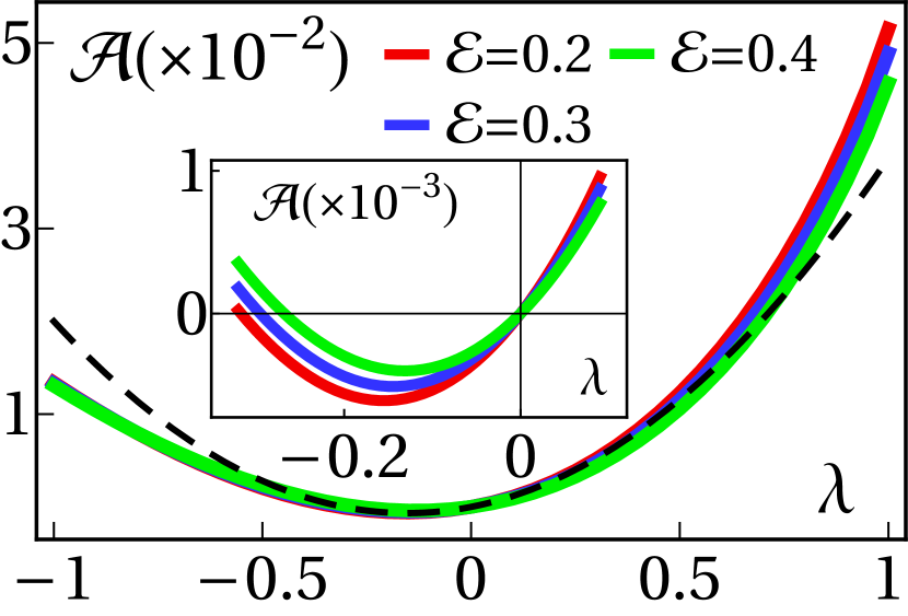
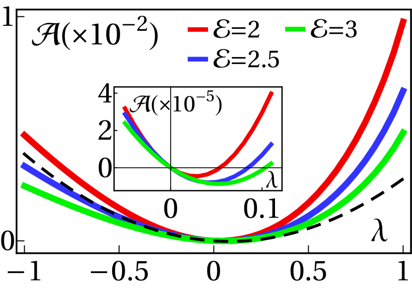
(a)      (b)      (c)

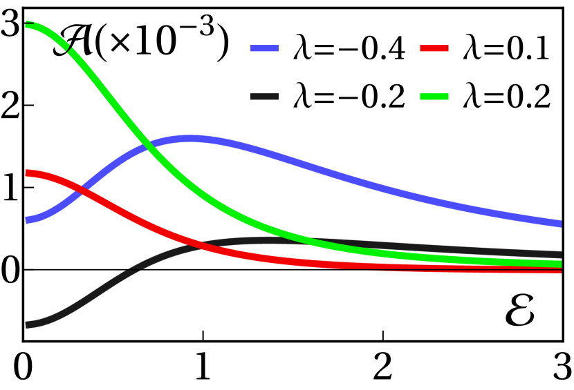
Figure 2: The FIF amplitude $\mathcal{A}$ as a function of $\lambda$ for (a) small and (b) large electric fields. Panel (c) shows $\mathcal{A}$ as a function of $\mathcal{E}$ for various values of $\lambda$. The solid lines correspond to the numerical evaluation of Eq. (Long-range fluctuation–induced forces in driven electrolytes), while the dashed lines in (a) and (b) are, respectively, the approximate forms for $\mathcal{E}\ll 1$ (independent of $\mathcal{E}$) and $\mathcal{E}\gg 1$ (computed for $\mathcal{E}=3$). The asymptotic expressions in Table. 1 reveal three distinct behaviors of $\mathcal{A}$ as a function of $\mathcal{E}$ (panel c): for $-0.31\lesssim\lambda<0$, the amplitude $\mathcal{A}$ is initially negative, crosses to positive values and falls off to zero for large $\mathcal{E}$; for $0<\lambda\lesssim 0.17$, the amplitude $\mathcal{A}$ is initially positive, crosses to negative values before approaching zero from below for large $\mathcal{E}$; and, finally, for $\lambda\lesssim-0.31$ or $\lambda\gtrsim 0.17$, $\mathcal{A}$ remains positive when $\mathcal{E}$ is varied.

Stress Tensor— The nonequilibrium pressure exerted on the boundaries can be calculated using the noise-averaged Maxwell stress $\langle\sigma_{ij}\rangle=\frac{\epsilon_{\rm in}}{2S_{d}}\left(2\langle\nabla_{i}\phi\,\nabla_{j}\phi\rangle-\delta_{ij}\langle(\nabla\phi)^{2}\rangle\right)$ . We assume no free charges on the boundaries, and hence the electrostatic boundary conditions are given by the continuity of the tangential electric field and the normal displacement field at both plates. Using image charges [51], the electric potential satisfying these conditions is obtained as $\phi(\bm{r})=\sum\limits_{n\in\mathbb{Z}}\int_{\bm{r}^{\prime}}\,\tfrac{\lambda^{n}\rho(\bm{r}^{\prime})Q}{\epsilon_{\rm in}(d-2)|\bm{r}-\bm{r}^{\prime}_{n}|^{d-2}}$ where $n$ indexes the image located at $\bm{r}^{\prime}_{n}$ (obtained from $\bm{r}^{\prime}$ by substituting $y^{\prime}\to y^{\prime}_{n}=2nH\pm y^{\prime}$), and $\lambda$ [as defined in Eq. (2)] represents the ratio of the successive image charges.

On substituting $\phi(\bm{r})$ into the Maxwell stress, performing the summation over image charges, and using Eq. (9), we arrive at Eq. (1) for the normal force on the plate at $y=H$ . The stress amplitude in Eq. (1) reads $\mathcal{A}=\lambda\int_{\bm{\nu}_{s}}\{\sum\limits_{n=0}^{\infty}\!\!{\vphantom{\sum}}^{\prime}\mathcal{R}_{n}(\lambda,\nu_{s})g(\mathcal{E},n,\bm{\nu}_{s})-\int_{0}^{\infty}\mathrm{d}n\,g(\mathcal{E},n,\bm{\nu}_{s})\}$, where we have defined $\mathcal{R}_{2k}=\mathcal{Y}_{-}$, $\mathcal{R}_{2k+1}=\mathcal{Y}_{+}$, $\mathcal{Y}_{\pm}\equiv\left(\frac{e^{\pi\nu_{s}}\pm 1}{e^{\pi\nu_{s}}\pm\lambda}\right)^{2}$, and $g=\tfrac{2^{1-d}\nu_{x}^{4}\bm{\nu}_{s}^{2}}{(\mathcal{E}^{2}\nu_{x}^{2}+n^{2}+\bm{\nu}_{s}^{2})(n^{2}+\bm{\nu}_{s}^{2})^{2}}$. For the $d=3$ case, we find [46]

$$\mathcal{A}(\mathcal{E},\lambda)=\frac{\lambda\zeta(3)}{16\pi}\frac{\mathcal{E}^{2}+2}{\mathcal{E}^{4}(\mathcal{E}^{2}+1)^{3/2}}+\frac{\mathcal{E}^{2}-4}{32\pi\mathcal{E}^{4}}\left[(\lambda-\frac{1}{\lambda})\mathrm{Li}_{2}(\lambda^{2})+\frac{1}{2}(\lambda+\frac{1}{\lambda})\mathrm{Li}_{3}(\lambda^{2})\right]+\frac{3\mathrm{Li}_{3}(\lambda^{2})}{32\pi\mathcal{E}^{2}}$$

$$\qquad+\frac{\lambda\pi}{16}\int_{0}^{2\pi}\mathrm{d}\theta\int_{0}^{\infty}\nu_{s}^{2}\mathrm{d}\nu_{s}\frac{\left[\mathcal{Y}_{-}(\lambda,\nu_{s})-1\right]\coth(\frac{\pi\nu_{s}}{2}\sqrt{\mathcal{E}^{2}\cos^{2}\theta+1})+\left[\mathcal{Y}_{+}(\lambda,\nu_{s})-1\right]\tanh(\frac{\pi\nu_{s}}{2}\sqrt{\mathcal{E}^{2}\cos^{2}\theta+1})}{\mathcal{E}^{4}\sqrt{\mathcal{E}^{2}\cos^{2}\theta+1}}$$ (10)

where ${\mathrm{Li}}_{n}(z)=\sum\limits_{k=1}^{\infty}\dfrac{z^{k}}{k^{n}}$ is the polylogarithm function. Figure 2 shows the variation of $\mathcal{A}$ as a function of $\lambda$ [Fig. 2(a) and Fig. 2(b)] and $\mathcal{E}$ [Fig. 2(c)] in $d=3$ dimensions, as obtained numerically from Eq. (Long-range fluctuation–induced forces in driven electrolytes). In Table 1, we also summarize the approximate forms for $\mathcal{A}$ in $d=3$ obtained from the suitable asymptotic expansion of Eq. (Long-range fluctuation–induced forces in driven electrolytes) in each regime [46]. These approximate forms are shown in Fig. 2(a) and Fig. 2(b) as dashed lines.

	$\mathcal{E}\ll 1$	$\mathcal{E}\gg 1$
$\lambda\!\ll\!1$	${\dfrac{9\left(4\zeta(5)+1\right)}{512\pi}\lambda^{2}\!+\!\dfrac{9\left(4\zeta(5)-1\right)}{1024\pi}\lambda}$	$\dfrac{\lambda(6\lambda-1)}{64\pi}\mathcal{E}^{-2}$
$\lambda\!=\!1$	$\dfrac{9\,\zeta(3)}{64\pi}$	$\dfrac{\zeta(3)}{8\pi}\mathcal{E}^{-2}$
$\lambda\!=\!-1$	$\dfrac{9\zeta(3)}{256\pi}$	$\dfrac{\zeta(3)}{16\pi}\mathcal{E}^{-2}$

Table 1: Leading order approximations of the dimensionless stress amplitude $\mathcal{A}(\mathcal{E},\lambda)$ in $d=3$, obtained from expanding Eq. (Long-range fluctuation–induced forces in driven electrolytes) (corrections are $\mathcal{O}(\mathcal{E}^{2})$ for $\mathcal{E}\ll 1$, and $\mathcal{O}(\mathcal{E}^{-4})$ for $\mathcal{E}\gg 1$). The relevant values of the Riemann zeta function are $\zeta(5)\approx 1.04$ and $\zeta(3)\approx 1.20$. (For derivations as well as asymptotic expressions in $d=2$, see Ref. [46].)

From Eq. (Long-range fluctuation–induced forces in driven electrolytes) and the asymptotic forms in Table. 1, we note that the FIF exhibits two different regimes for weak and strong applied electric fields: for weak fields ($\mathcal{E}\ll 1$), the force scales as $E^{4}$, and it is proportional to the inverse temperature ($\propto\beta$) and the inverse average density squared ($\propto 1/C_{0}^{2}$); for strong fields ($\mathcal{E}\gg 1$), the force scales as $E^{2}$, and it is proportional to the inverse average density ($\propto 1/C_{0}$) and becomes independent of temperature. (Note that the second line in Eq. (Long-range fluctuation–induced forces in driven electrolytes) is a subleading correction for $\mathcal{E}\gg 1$.) Fig. 2 also shows that the sign of the force amplitude can change with the applied electric field: for $\lambda\ll 1$ (i.e. small dielectric contrast), the amplitude $\mathcal{A}$ can become negative which, remarkably, indicates a repulsive FIF between boundaries that enclose the driven electrolyte. For moderate values of the dielectric contrast $\lambda$, on the other hand, the force remains attractive with a positive amplitude.

Concluding Remarks— We showed that the effective anisotropy introduced by the external electric field renders the steady-state density and charge fluctuations in a driven electrolyte long-range correlated, in contrast to the screened correlations in thermal equilibrium. These nonequilibrium correlations give rise to long-range FIFs on external objects and boundaries immersed in the driven electrolyte. For neutral boundaries parallel with the external field (Fig. 1), our results show that the force varies non-monotonically with the electric field and the dielectric contrast; notably, with symmetric boundaries, the long-range FIF can be tuned to be attractive or repulsive with different amplitudes by varying the relevant parameters. We note the present setup gives an independent mechanism for tuning nonequilibrium FIFs from the one in Ref. [19], and investigating the interplay of the two effects forms an interesting direction for future studies.

This work highlights a generic mechanism through which nonequilibrium fluctuations can give rise to long-range forces in driven charged systems. A similar mechanism may also be relevant for concentrated electrolytes where it has been suggested that the “defects” are the main charge carriers [54], and it may also be applicable to ionic liquids where mainly the “free ions” participate in conduction and screening processes [55, 56]. Long-ranged forces have recently been observed in a number of experimental settings [25, 26] where oscillatory electric fields are applied to charged solutions. Our preliminary analysis shows that the FIF introduced here can help to understand the experimentally observed dynamical features; we plan to extend our results to include time-dependent electric fields and different boundary conditions. In addition, the model used here relies on the linearization of the stochastic dynamics which is applicable to strong electrolytes far from phase transitions and where the Gaussian scalings hold [46]. We plan to perform a more rigorous treatment of the nonlinearities using renormalization group (RG) techniques which have recently been applied to similar dynamics in the context of chemotaxis [57].

Acknowledgments – The authors thank A. Gambassi, A. Maciołek, S. Dietrich, M. Bier, and M. Gross for pointing out the difference in screening of the external field with perpendicular setups and for bringing the references on critical Casimir force to our attention. We also thank Susan Perkin for helpful discussions. S.M. acknowledges the support of the Clarendon Fund and St John’s College Kendrew Scholarship from the University of Oxford. This work was supported by the Max Planck Society.

References

- Kardar and Golestanian [1999] M. Kardar and R. Golestanian, The “friction” of vacuum, and other fluctuation-induced forces, Rev. Mod. Phys. 71, 1233 (1999).
- Gambassi [2009] A. Gambassi, The Casimir effect: From quantum to critical fluctuations, J. Phys.: Conf. Ser. 161, 012037 (2009).
- Jancovici and Šamaj [2004] B. Jancovici and L. Šamaj, Screening of classical Casimir forces by electrolytes in semi-infinite geometries, J. Stat. Mech.: Theory Exp. 2004 (08), P08006.
- Lee et al. [2018] A. A. Lee, J.-P. Hansen, O. Bernard, and B. Rotenberg, Casimir force in dense confined electrolytes, Mol. Phys. 116, 3147 (2018).
- French et al. [2010] R. H. French, V. A. Parsegian, R. Podgornik, R. F. Rajter, A. Jagota, J. Luo, D. Asthagiri, M. K. Chaudhury, Y.-m. Chiang, S. Granick, S. Kalinin, M. Kardar, R. Kjellander, D. C. Langreth, J. Lewis, S. Lustig, D. Wesolowski, J. S. Wettlaufer, W.-Y. Ching, M. Finnis, F. Houlihan, O. A. von Lilienfeld, C. J. van Oss, and T. Zemb, Long range interactions in nanoscale science, Rev. Mod. Phys. 82, 1887 (2010).
- Casimir [1948] H. B. Casimir, On the attraction between two perfectly conducting plates, Proc. Kon. Ned. Akad. Wet. 51, 793 (1948).
- Fisher and Gennes [1978] M. E. Fisher and P. Gennes, Wall phenomena in a critical binary mixture, C. R. Acad. Sc. Paris B 287, 207 (1978).
- Hertlein et al. [2008] C. Hertlein, L. Helden, A. Gambassi, S. Dietrich, and C. Bechinger, Direct measurement of critical Casimir forces, Nature 451, 172 (2008).
- Maciołek and Dietrich [2018] A. Maciołek and S. Dietrich, Collective behavior of colloids due to critical Casimir interactions, Rev. Mod. Phys. 90, 045001 (2018).
- Garrido et al. [1990] P. L. Garrido, J. L. Lebowitz, C. Maes, and H. Spohn, Long-range correlations for conservative dynamics, Phys. Rev. A 42, 1954 (1990).
- Grinstein et al. [1990] G. Grinstein, D.-H. Lee, and S. Sachdev, Conservation laws, anisotropy, and “self-organized criticality” in noisy nonequilibrium systems, Phys. Rev. Lett. 64, 1927 (1990).
- Hwa and Kardar [1989] T. Hwa and M. Kardar, Dissipative transport in open systems: An investigation of self-organized criticality, Phys. Rev. Lett. 62, 1813 (1989).
- Najafi and Golestanian [2004] A. Najafi and R. Golestanian, Forces induced by nonequilibrium fluctuations: The Soret-Casimir effect, EPL 68, 776 (2004).
- Aminov et al. [2015] A. Aminov, Y. Kafri, and M. Kardar, Fluctuation-induced forces in nonequilibrium diffusive dynamics, Phys. Rev. Lett. 114, 230602 (2015).
- Rohwer et al. [2017] C. M. Rohwer, M. Kardar, and M. Krüger, Transient Casimir forces from quenches in thermal and active matter, Phys. Rev. Lett. 118, 015702 (2017).
- Rohwer et al. [2018] C. M. Rohwer, A. Solon, M. Kardar, and M. Krüger, Nonequilibrium forces following quenches in active and thermal matter, Phys. Rev. E 97, 032125 (2018).
- Ray et al. [2014] D. Ray, C. Reichhardt, and C. J. O. Reichhardt, Casimir effect in active matter systems, Phys. Rev. E 90, 013019 (2014).
- Dean and Podgornik [2014] D. S. Dean and R. Podgornik, Relaxation of the thermal Casimir force between net neutral plates containing Brownian charges, Phys. Rev. E 89, 032117 (2014).
- Dean et al. [2016] D. S. Dean, B.-S. Lu, A. C. Maggs, and R. Podgornik, Nonequilibrium Tuning of the Thermal Casimir Effect, Phys. Rev. Lett. 116, 240602 (2016).
- Perkin [2012] S. Perkin, Ionic liquids in confined geometries, Physical Chemistry Chemical Physics 14, 5052 (2012).
- Siwy and Fuliński [2002] Z. Siwy and A. Fuliński, Fabrication of a synthetic nanopore ion pump, Phys. Rev. Lett. 89, 198103 (2002).
- Schoch et al. [2008] R. B. Schoch, J. Han, and P. Renaud, Transport phenomena in nanofluidics, Rev. Mod. Phys. 80, 839 (2008).
- Aidley and Stanfield [1996] D. J. Aidley and P. R. Stanfield, Ion channels: molecules in action (Cambridge University Press, 1996).
- Martinac [2004] B. Martinac, Mechanosensitive ion channels: molecules of mechanotransduction, J. Cell Sci. 117, 2449 (2004).
- Perez-Martinez and Perkin [2019] C. S. Perez-Martinez and S. Perkin, Surface forces generated by the action of electric fields across liquid films, Soft Matter 15, 4255 (2019).
- Richter et al. [2020] L. Richter, P. J. Żuk, P. Szymczak, J. Paczesny, K. M. Bkak, T. Szymborski, P. Garstecki, H. A. Stone, R. Hołyst, and C. Drummond, Ions in an ac electric field: Strong long-range repulsion between oppositely charged surfaces, Phys. Rev. Lett. 125, 056001 (2020).
- Israelachvili [2011] J. N. Israelachvili, Intermolecular and surface forces (Academic press, 2011).
- Grinstein [1991] G. Grinstein, Generic scale invariance in classical nonequilibrium systems, J. Appl. Phys. 69, 5441 (1991).
- Täuber [2014] U. C. Täuber, Critical dynamics: a field theory approach to equilibrium and non-equilibrium scaling behavior (Cambridge University Press, 2014).
- Note [1] In setups where the electric field is applied perpendicular to the (charged) boundaries, the renormalization of the applied field due to screening effects should be taken into account.
- Mohry et al. [2010] T. Mohry, A. Maciołek, and S. Dietrich, Crossover of critical Casimir forces between different surface universality classes, Phys. Rev. E 81, 061117 (2010).
- Tröndle et al. [2010] M. Tröndle, S. Kondrat, A. Gambassi, L. Harnau, and S. Dietrich, Critical Casimir effect for colloids close to chemically patterned substrates, J. Chem. Phys. 133, 074702 (2010).
- Vasilyev et al. [2011] O. Vasilyev, A. Maciołek, and S. Dietrich, Critical Casimir forces for Ising films with variable boundary fields, Phys. Rev. E 84, 041605 (2011).
- Bier et al. [2011] M. Bier, A. Gambassi, M. Oettel, and S. Dietrich, Electrostatic interactions in critical solvents, EPL 95, 60001 (2011).
- Pousaneh et al. [2014] F. Pousaneh, A. Ciach, and A. Maciołek, How ions in solution can change the sign of the critical Casimir potential, Soft Matter 10, 470 (2014).
- Onsager and Fuoss [1932] L. Onsager and R. M. Fuoss, Irreversible processes in electrolytes. diffusion, conductance and viscous flow in arbitrary mixtures of strong electrolytes, J. Phys. Chem. 36, 2689 (1932).
- Zorkot et al. [2016] M. Zorkot, R. Golestanian, and D. J. Bonthuis, The power spectrum of ionic nanopore currents: the role of ion correlations, Nano Lett. 16, 2205 (2016).
- Démery and Dean [2016] V. Démery and D. S. Dean, The conductivity of strong electrolytes from stochastic density functional theory, J. Stat. Mech.: Theory Exp. 2016 (2), 023106.
- Note [2] The hydrodynamic interactions can become relevant in a concentrated electrolyte (where the hydrodynamic radii of the particles become comparable with interparticle distances) or in extreme confinements. These are not the focus of this letter.
- Dean [1996] D. S. Dean, Langevin equation for the density of a system of interacting Langevin processes, J. Phys. A 29, L613 (1996).
- Kawasaki [1994] K. Kawasaki, Stochastic model of slow dynamics in supercooled liquids and dense colloidal suspensions, Physica A 208, 35 (1994).
- te Vrugt et al. [2020] M. te Vrugt, H. Löwen, and R. Wittkowski, Classical dynamical density functional theory: from fundamentals to applications, Adv. Phys. 69, 121 (2020).
- Démery et al. [2014] V. Démery, O. Bénichou, and H. Jacquin, Generalized Langevin equations for a driven tracer in dense soft colloids: construction and applications, New J. Phys. 16, 053032 (2014).
- Zorkot and Golestanian [2018] M. Zorkot and R. Golestanian, Current fluctuations across a nano-pore, J. Phys. Condens. Matter 30, 134001 (2018).
- Poncet et al. [2017] A. Poncet, O. Bénichou, V. Démery, and G. Oshanin, Universal long ranged correlations in driven binary mixtures, Phys. Rev. Lett. 118, 118002 (2017).
- Note [101] See Supplemental Material at [URL will be inserted by publisher] which contains more details on scaling analysis, correlation functions, and calculation and analysis of the stress tensor in and dimensions.
- Note [102] We have discarded the noise when substituting Eq. (5\@@italiccorr) into Eq. (3\@@italiccorr), as it is negligible with respect to due to the presence of an additional gradient operator.
- Note [103] The difference in mobilities, however, has important implications on the steady electric field in the presence of oscillatory external driving, see Ref. [58].
- Barton and Barton [1989] G. Barton and G. Barton, Elements of Green’s functions and propagation: potentials, diffusion, and waves (Oxford University Press, 1989).
- Note [104] Using the Maxwell stress in this nonequilibrium setting is justified as it derives from the electrostatic force density [59] in a similar way as the nonequilibrium Irving–Kirkwood formula is constructed from microscopic forces [60, 61].
- Jackson [2007] J. D. Jackson, Classical Electrodynamics (John Wiley & Sons, 2007).
- Note [105] For , the potential is given by the logarithmic Coulomb form, while the Maxwell stress formula remains unchanged.
- Note [106] The force exerted on the boundary has the same magnitude and is in the opposite direction.
- Lee et al. [2017] A. A. Lee, C. S. Perez-Martinez, A. M. Smith, and S. Perkin, Scaling analysis of the screening length in concentrated electrolytes, Phys. Rev. Lett. 119, 026002 (2017).
- Lee et al. [2015] A. A. Lee, D. Vella, S. Perkin, and A. Goriely, Are room-temperature ionic liquids dilute electrolytes?, J. Phys. Chem. Lett. 6, 159 (2015).
- Feng et al. [2019] G. Feng, M. Chen, S. Bi, Z. A. H. Goodwin, E. B. Postnikov, N. Brilliantov, M. Urbakh, and A. A. Kornyshev, Free and bound states of ions in ionic liquids, conductivity, and underscreening paradox, Phys. Rev. X 9, 021024 (2019).
- Mahdisoltani et al. [2020] S. Mahdisoltani, R. B. A. Zinati, C. Duclut, A. Gambassi, and R. Golestanian, Nonequilibrium polarity-induced mechanism for chemotaxis: emergent Galilean symmetry and exact scaling exponents, arXiv:1911.08115 (2020).
- Amrei et al. [2018] S. H. Amrei, S. C. Bukosky, S. P. Rader, W. D. Ristenpart, and G. H. Miller, Oscillating electric fields in liquids create a long-range steady field, Phys. Rev. Lett. 121, 185504 (2018).
- Woodson and Melcher [1968] H. H. Woodson and J. R. Melcher, Electromechanical dynamics (Wiley, 1968).
- Irving and Kirkwood [1950] J. Irving and J. G. Kirkwood, The statistical mechanical theory of transport processes. IV. The equations of hydrodynamics, J. Chem. Phys. 18, 817 (1950).
- Krüger et al. [2018] M. Krüger, A. Solon, V. Démery, C. M. Rohwer, and D. S. Dean, Stresses in non-equilibrium fluids: Exact formulation and coarse-grained theory, J. Chem. Phys. 148, 084503 (2018).