Inverse design of dissipative quantum steady-states with implicit differentiation

Abstract

Inverse design of a property that depends on the steady-state of an open quantum system is commonly done by grid-search type of methods. In this paper we present a new methodology that allows us to compute the gradient of the steady-state of an open quantum system with respect to any parameter of the Hamiltonian using the implicit differentiation theorem. As an example, we present a simulation of a spin-boson model where the steady-state solution is obtained using Redfield theory.

1 Introduction

The field of open quantum systems (OQS) is focused on studying the interaction of a system (S) with its surroundings, typically referred to as the bath (B) (Breuer and Petruccione, 2002). The Hamiltonian for the complete problem is defined as the sum of the isolated system Hamiltonian, $H_{S}$, the bath that surrounds the system, $H_{B}$, and the interaction between the system and the bath, $H_{SB}$,

$$H=H_{S}+H_{B}+H_{SB}.$$ (1)

For physical problems the bath is often represented as a continuum that describes the vibrational or solvent degrees of freedom. Given the large dimensionality of the composite Hilbert space of such systems, it is common to construct a reduced representation by tracing out the bath degrees of freedom, $\rho_{S}=\text{Tr}_{B}[\rho]$. Here, we refer to $\rho_{S}$ as the reduced density matrix (RDM) and $\rho$ is the density matrix of the complete system.

In OQS, one is usually interested in the dissipative effects the bath induces in the system over time. However, for many OQS the properties of interest are related to the steady-state (SS) of the system ($\rho^{ss}$), $\;d\rho(t)/dt=0$; for example, energy transfer efficiency in biological systems excited by natural incoherent light (Tscherbul and Brumer, 2014, 2015; Pachón et al., 2017) and the performance of quantum heat engines/refrigerators (Kilgour and Segal, 2018; Linden et al., 2010). Here, we propose a novel numerical algorithm to compute the gradient of the steady-state of an OQS with respect to any parameter of the Hamiltonian ($\bm{\theta}_{i}$) using implicit differentiation, $\partial\rho^{ss}/\partial\bm{\theta}_{i}$, allowing us to tackle problems related to inverse design and sensitivity analysis.

In the following sections, we discuss how as an example, we differentiate the steady-state of the spin-boson (SB) model with respect to any parameter using an ordinary differential equation solver and implicit differentiation.

2 Differentiation of the steady-state

Conditioned on initial values $\rho(t_{0})\in\mathbb{C}^{d}$ and free parameters $\bm{\theta}$, let $\rho(t)\in\mathbb{C}^{d}$ be the solution to a homogeneous dynamical system parameterized by an ordinary differential equation (ODE) $\frac{d\rho}{dt}=f(\rho,\bm{\theta})$ where $d$ is the dimensionality of the RDM. In optimization, we want to compute the gradient of the steady state with respect to the parameters $\bm{\theta}$. Let us denote $\rho^{ss}$ as the steady-state, which satisfies $f(\rho^{ss},\bm{\theta})=0$.

We can solve for $\rho^{ss}$ by running an appropriate ODE solver for a sufficiently long period of time. However, differentiating through the internals of the ODE solver is computationally expensive as it requires storing all intermediate quantities of the solver. The adjoint method for computing gradients of ODE solutions requires either the trajectory $\rho(t)$ to be stored in memory or solving $\rho(t)$ in reverse time, which uses constant memory (Chen et al., 2018). However, since we are interested in $\rho^{ss}$, the reversing approach is not applicable as the steady state, once reached, cannot be reversed. Instead, since $\rho^{ss}$ is the solution of a fixed point problem, the Jacobian $\frac{d\rho^{ss}}{d\bm{\theta}}$ can be expressed using the implicit function theorem (Krantz and Parks, 2012),

$$\frac{d\rho^{ss}}{d\bm{\theta}}=-\left(\frac{df(\rho^{ss},\bm{\theta})}{d\rho}\right)^{-1}\left[\frac{df(\rho^{ss},\bm{\theta})}{d\bm{\theta}}\right].$$ (2)

We show that it is possible to compute this gradient, i.e. Eq. (2), using constant memory cost, and without the need to know how $\rho^{ss}$ is computed as long as it satisfies the steady state criterion, i.e. $f(\rho^{ss},\bm{\theta})=0$.

For this work, we would also have a scalar loss function ${\cal L}(\bm{\theta},\rho^{ss})$ that we wish to minimize. Here, the gradient with respect to parameters can be factored with the chain rule $\frac{d{\cal L}}{d\rho^{ss}}\frac{d\rho^{ss}}{d\bm{\theta}}$. In general, we’re interested in vector-Jacobian products of the form $v\frac{d\rho^{ss}}{d\bm{\theta}}$ where $v$ is any vector. In automatic differentiation libraries such as jax (Bradbury et al., 2018), we can easily compute vector-Jacobian products for large systems but recovering the full Jacobian is more costly.

Computing a vector-Jacobian product using, Eq. (2), requires solving $vJ^{-1}$ where $J=\left(\frac{df(\rho^{ss},\bm{\theta})}{d\rho}\right)^{-1}$. For large systems where $J$ cannot be tractably computed, we compute $vJ^{-1}$ by recognizing that it is the steady-state solution of the ODE $\frac{dy}{dt}=yJ-v$. Notably, simulating this ODE only requires vector-Jacobian products, which are inexpensive in automatic differentiation libraries. In the following sections we illustrate how inverse design and sensitivity analysis are possible for dissipative quantum systems by differentiating through the steady state of a Spin-Boson model.

3 Example: Spin-Boson model

In the field of OQS, the SB Hamiltonian (Thoss et al., 2001) is a standard model used to describe a wide variety of physical phenomena (Breuer and Petruccione, 2002; Leggett et al., 1987) including electron transfer (Egorova et al., 2003), heat transport (Xu and Cao, 2016), and energy transfer (Liu and Segal, 2019; Jung and Brumer, 2020). The total Hamiltonian is,

$$H_{S}=\frac{\varepsilon}{2}\sigma_{z}+\frac{\Delta}{2}\sigma_{x},\;\;\;\;H_{B}=\sum_{k}\omega_{k}b_{k}^{\dagger}b_{k},\;\;\;\;H_{SB}=\sigma_{z}\sum_{k}\lambda_{k}(b_{k}^{\dagger}+b_{k}),$$ (3)

where $b_{k}^{\dagger}$ ($b_{k}$) is the creation (annihilation) operator of mode $k$ in the bath, $\sigma_{z}$ and $\sigma_{x}$ are Pauli matrices, and $\{\lambda_{k}\}$ are the coupling strength parameters, and $\varepsilon$ and $\Delta$ are system parameters.

The exact equation of motion (Nakajima, 1958; Zwanzig, 1960) for the RDM is not practical to solve since one requires knowledge of the interacting system-bath dynamics. Redfield theory (RT) (Redfield, 1965; Palenberg et al., 2001) is a practical alternative for regimes in which the system-bath coupling is weak, i.e. $\{\lambda_{k}\}\ll 1$. The RT equations of motions written in the system eigenbasis are,

$$\frac{\partial\rho_{\mu,\nu}(t)}{\partial t}=-i\omega_{\mu,\nu}\rho_{\mu,\nu}(t)+\sum_{\kappa,\lambda}R_{\mu,\nu,\kappa,\lambda}\;\rho_{\kappa,\lambda}(t),$$ (4)

where $[\mu,\nu,\kappa,\lambda]$ are the index of the eigenstates of $H_{S}$, i.e. they satisfy $H_{S}|\mu\ \rangle=\varepsilon_{\mu}|\mu\rangle$, and $\omega_{\mu,\nu}$ is the difference between eigenvalues $\varepsilon_{\mu}$ and $\varepsilon_{\nu}$. $R_{\mu,\nu,\kappa,\lambda}$ are the Redfield tensors which describe the interaction of the system and bath and are given by,

$$R_{\mu,\nu,\kappa,\lambda}=\Gamma^{+}_{\lambda,\nu,\mu,\kappa}+\Gamma^{-}_{\lambda,\nu,\mu,\kappa}-\delta_{\nu,\lambda}\sum_{\alpha}\Gamma^{+}_{\mu,\alpha,\alpha,\kappa}-\delta_{\mu,\kappa}\sum_{\alpha}\Gamma^{+}_{\lambda,\alpha,\alpha,\nu},$$ (5)

which contain the transition rates,

$$\Gamma^{+}_{\lambda,\nu,\mu,\kappa} = \langle\lambda|\sigma_{z}|\nu\rangle\langle\mu|\sigma_{z}|\kappa\rangle\int_{0}^{\infty}\mathrm{d}\tau F(\tau)e^{-i\omega_{\mu,\kappa}\tau},$$ (6)

$$\Gamma^{-}_{\lambda,\nu,\mu,\kappa} = \langle\lambda|\sigma_{z}|\nu\rangle\langle\mu|\sigma_{z}|\kappa\rangle\int_{0}^{\infty}\mathrm{d}\tau F^{*}(\tau)e^{-i\omega_{\lambda,\nu}\tau},$$ (7)

that are in turn comprised of the bath correlation function,

$$F(\tau)=\int_{0}^{\infty}\mathrm{d}\omega\;g(\omega)\left[\coth(\beta\omega/2)\cos(\omega\tau)-i\sin(\omega\tau)\right].$$ (8)

$g(\omega)$ is the spectral density function, $g(\omega)=\eta\omega^{s}\omega_{c}^{1-s}e^{-\omega/\omega_{c}}$; for this work we used the super Ohmic form of $s=3$. $\eta$ is the bath friction parameter that is on the order of $\lambda_{k}^{2}$ and $\beta$ is the inverse temperature.

4 Results

4.1 Sensitivity analysis

One of the most studied observables for the SB model is the population difference at equilibrium, $\langle\sigma_{z}\rangle=\text{Tr}[\sigma_{z}\rho^{ss}]$. Fig. (1) illustrates the change of $\langle\sigma_{z}\rangle$ with respect to bath parameters $\beta$, $\eta$ and the system parameters $\Delta$. For all calculations we used $w_{c}=1$, $\varepsilon=0.1$ and the initial density matrix was taken to be

$$\rho_{S}(t_{0})=\begin{pmatrix}\frac{3}{4}&-i\frac{\sqrt{3}}{4}\\ i\frac{\sqrt{3}}{4}&\frac{1}{4}\end{pmatrix}.$$ (9)

We can observe that $\langle\sigma_{z}\rangle$ is independent of $\beta$ and $\eta$, as the gradients are effectively zero. However, $\frac{\partial\langle\sigma_{z}\rangle}{\partial\Delta}$ is nonzero which confirms the effect $\Delta$ has in $\langle\sigma_{z}\rangle$.

While finite differences with respect to $\beta$, $\eta$, and $\Delta$ can be computed one at a time, this requires $\mathcal{O}(d)$ evaluations of the steady state. The automatic differentiation process discussed in Section 2 allows us to compute analytical derivatives for all parameters simultaneously with just one evaluation of the steady-state.

To construct the Redfield tensors we must know the eigenvalues and eigenstates of $H_{S}$ beforehand. As $H_{S}$ is not diagonal for $\Delta>0$, the eigenvalues and eigenstates do not have trivial analytical solutions. To compute these, we used jax’s eigendecomposition. This ensures this method can be applied to arbitrary systems.

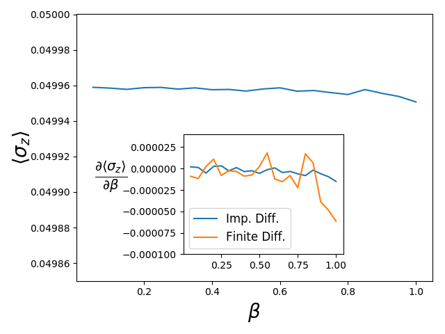
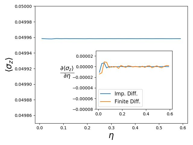
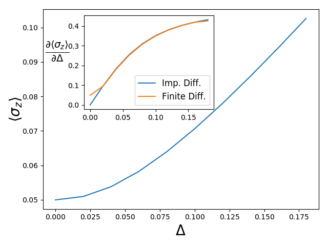
Figure 1: $\langle\sigma_{z}\rangle=\text{Tr}[\sigma_{z}\rho^{ss}]$ as a function of different parameters, $\beta$, $\eta$ and $\Delta$. The inset of each figure compares the gradient computed with Eq. (2) (blue solid curve) and finite differences (orange solid curve). For all calculations, except for the parameter in play, we used $\beta=0.1$, $\eta=0.01$, $w_{c}=1$, $\varepsilon=0.1$, and $\Delta=0$. The initial density matrix used was $\rho_{S}(t_{0})=[3/4,-i\frac{\sqrt{3}}{4},i\frac{\sqrt{3}}{4},1/4]$ (Eq. 9).

4.2 Inverse design for system’s Hamiltonian

Gradient based methods have proven to be powerful numerical tools to find the minimizer of loss functions. Given the possibility to compute quantities like $\partial{\cal L}/\partial\theta_{i}$, we could reformulate the inverse design problem into an optimization one. For example, what values of $\varepsilon$ and $\Delta$ reproduce a target observable. In order to do so we define an error function, e.g., ${\cal L}(\varepsilon,\Delta)=\left\|\langle\sigma_{z}\rangle-\hat{\langle\sigma_{z}\rangle}\right\|_{2}$.

Fig. 2 illustrates how gradient-based methods can be used to search for the optimal values of $\varepsilon$ and $\Delta$ that reproduce a target $\langle\sigma_{z}\rangle$; as a proof of principle calculation we used $\varepsilon=0.1$, $\Delta=0$ where $\langle\sigma_{z}\rangle=0.04995847$. For these simulations we fixed the values of $\beta$ and $\eta$. Furthermore, in Table 1 we report the values of $\varepsilon$ and $\Delta$ for 5 different optimizations. To minimize ${\cal L}$ we used the Adam algorithm, which is a first-order gradient-based optimization algorithm (Kingma and Ba, 2017).

Table 1:  

$\varepsilon$	$\Delta$	$\langle\sigma_{z}\rangle$	${\cal L}$
0.0835	0.0578	0.049947	1.2E-5
0.0867	0.0526	0.049942	1.6E-5
0.0739	0.0692	0.049913	4.5E-5
0.0490	0.0809	0.049921	3.8E-5
0.0822	0.0597	0.049940	1.9E-5

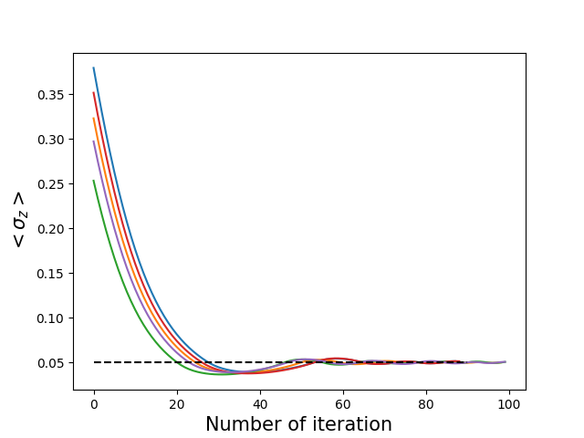
(a)

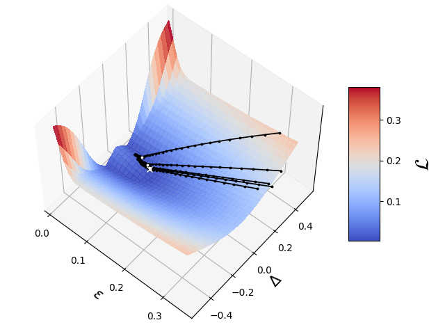
(b)

Figure 2: We optimize the parameters of $H_{S}$, $\varepsilon$ and $\Delta$, with respect to a target $\hat{\langle\sigma_{z}\rangle}$ computed with $\varepsilon=0.1$ and $\Delta=0$. We used the Adam optimization algorithm to minimize ${\cal L}(\varepsilon,\Delta)=\left\|\langle\sigma_{z}\rangle-\hat{\langle\sigma_{z}\rangle}\right\|_{2}$. (a) The value of $\langle\sigma_{z}\rangle$ at each iteration of the optimization routine for different random initialization. The black-dashed curves is the target $\langle\sigma_{z}\rangle$. (b) The iterations of the optimization procedure in the parameter space for different random initialization. The white-$x$ symbol represents the target set of parameters and the white-$\bullet$ is the set of parameters found at 100th iteration of the Adam algorithm. $\frac{\partial{\cal L}}{\partial\varepsilon}$ and $\frac{\partial{\cal L}}{\partial\Delta}$ used in the Adam optimizer were computed with Eq. (2). For all calculations, we used $\beta=0.1$, $\eta=0.01$, $w_{c}=1$ and $\rho(t_{0})$ was the same as in Fig. (1). The learning rate was set to 0.1, and we parameterized $\varepsilon$ and $\Delta$ to be strictly positive by using the softplus function.

5 Summary

We have presented a novel numerical methodology capable of computing the gradient of quantum observables of the form $\langle\hat{O}\rangle=\text{Tr}[\hat{O}\rho^{ss}]$, with respect to any parameter of the Hamiltonian. As we stated, this procedure does not depend on the numerical procedure used to solve for $\rho^{ss}$ and it uses constant memory. By computing the gradient of $\langle\sigma_{z}\rangle$, for the particular parameter set and model used we found an independence of $\langle\sigma_{z}\rangle$ with respect to the bath parameters. $\langle\sigma_{z}\rangle$ increases as a function of $\Delta$ and the gradient computed with Eq. (2) matches the gradient computed with finite differences.

Inverse design for physical systems is one of the most common applications for gradient-based search algorithms. We have demonstrated that the Adam algorithm can be used to find the optimal values of $\varepsilon$ and $\Delta$ that reproduce a target $\langle\sigma_{z}\rangle$.

For all the results presented here, we considered a unique $\rho_{S}(t_{0})$; however, one can apply this technique to search for the optimal $\rho_{S}(t_{0})$ given a scalar observable that depends on the steady-state. For example, in the SB model one can define $\bm{\theta}$ to include the initial values of the RDM to study the dependence of the SS on initial conditions.

6 Broader Impact

Open quantum systems appear in many areas in physics. Our work can potentially be used for designing quantum heat engines or materials with specific desirable properties. This work itself is unlikely to have immediate ethical issues.

References

- Bradbury et al. [2018] J. Bradbury, R. Frostig, P. Hawkins, M. J. Johnson, C. Leary, D. Maclaurin, and S. Wanderman-Milne. JAX: composable transformations of Python+NumPy programs, 2018.
- Breuer and Petruccione [2002] H. P. Breuer and F. Petruccione. The theory of open quantum systems. Oxford University Press, Great Clarendon Street, 2002.
- Chen et al. [2018] R. T. Q. Chen, Y. Rubanova, J. Bettencourt, and D. K. Duvenaud. Neural ordinary differential equations. In Advances in neural information processing systems, pages 6571–6583, 2018.
- Egorova et al. [2003] D. Egorova, M. Thoss, W. Domcke, and H. Wang. Modeling of ultrafast electron-transfer processes: Validity of multilevel redfield theory. J. Chem. Phys., 119(5):2761–2773, 2003.
- Jung and Brumer [2020] K. A. Jung and P. Brumer. Energy transfer under natural incoherent light: Effects of asymmetry on efficiency. J. Chem. Phys., 153(11):114102, 2020.
- Kilgour and Segal [2018] M. Kilgour and D. Segal. Coherence and decoherence in quantum absorption refrigerators. Phys. Rev. E, 98:012117, 2018.
- Kingma and Ba [2017] D. P. Kingma and J. Ba. Adam: A method for stochastic optimization. arXiv, 1412.6980, 2017.
- Krantz and Parks [2012] S. G. Krantz and H. R. Parks. The implicit function theorem: history, theory, and applications. Springer Science & Business Media, 2012.
- Leggett et al. [1987] A. J. Leggett, S. Chakravarty, A. T. Dorsey, M. P. A. Fisher, Anupam Garg, and W. Zwerger. Dynamics of the dissipative two-state system. Rev. Mod. Phys., 59:1–85, 1987.
- Linden et al. [2010] N. Linden, S. Popescu, and P. Skrzypczyk. How small can thermal machines be? the smallest possible refrigerator. Phys. Rev. Lett., 105:130401, 2010.
- Liu and Segal [2019] J. Liu and D. Segal. Interplay of direct and indirect charge-transfer pathways in donor–bridge–acceptor systems. J. Phys. Chem. B, 123(28):6099–6110, 2019.
- Nakajima [1958] S. Nakajima. On quantum theory of transport phenomena. Progress of Theoretical Physics, 20(6):948–959, 1958.
- Pachón et al. [2017] L. A. Pachón, J. D. Botero, and P. Brumer. Open system perspective on incoherent excitation of light-harvesting systems. J. Phys. B: At. Mol. Opt. Phys, 50(18):184003, 2017.
- Palenberg et al. [2001] M. A. Palenberg, R. J. Silbey, C. Warns, and P. Reineker. Local and nonlocal approximation for a simple quantum system. J. Chem. Phys., 114(10):4386, 2001.
- Redfield [1965] A. G. Redfield. The theory of relaxation processes. In J. S. Waugh, editor, Advances in Magnetic Resonance, volume 1 of Advances in Magnetic and Optical Resonance, pages 1 – 32. Academic Press, 1965.
- Thoss et al. [2001] M. Thoss, H. Wang, and W. H. Miller. Self-consistent hybrid approach for complex systems: Application to the spin-boson model with debye spectral density. J. Chem. Phys., 115(7):2991–3005, 2001.
- Tscherbul and Brumer [2014] T. V. Tscherbul and P. Brumer. Long-lived quasistationary coherences in a -type system driven by incoherent light. Phys. Rev. Lett., 113:113601, 2014.
- Tscherbul and Brumer [2015] T. V. Tscherbul and P. Brumer. Partial secular bloch-redfield master equation for incoherent excitation of multilevel quantum systems. J. Chem. Phys., 142(10):104107, 2015.
- Xu and Cao [2016] D. Xu and J. Cao. Non-canonical distribution and non-equilibrium transport beyond weak system-bath coupling regime: A polaron transformation approach. Frontiers of Physics, 11(4), 2016.
- Zwanzig [1960] R. Zwanzig. Ensemble method in the theory of irreversibility. J. Chem. Phys., 33(5):1338–1341, 1960.