Inverse Problems for Semiconductors: Models and Methods

Abstract

We consider the problem of identifying discontinuous doping profiles in semiconductor devices from data obtained by different models connected to the voltage-current map. Stationary as well as transient settings are discussed and a framework for the corresponding inverse problems is established. Numerical implementations for the so-called stationary unipolar and stationary bipolar cases show the effectiveness of a level set approach to tackle the inverse problem.

1 Introduction

The mathematical model

The starting point of the mathematical model discussed in this paper is the system of drift diffusion equations (see (1a) – (1f) below). This system of equations, derived more than fifty years ago vRo (50), is the most widely used to describe semiconductor devices. For the current state of technology, this system represents an accurate compromise between efficient numerical solvability of the mathematical model and realistic description of the underlying physics Mar (86); MRS (90); Sel (84).

The name drift diffusion equations of semiconductors originates from the type of dependence of the current densities on the carrier densities and the electric field. The current densities are the sums of drift terms and diffusion terms. It is worth mentioning that, with the increased miniaturization of semiconductor devices, one comes closer and closer to the limits of validity of the drift diffusion equation. This is due to the fact that in ever smaller devices the assumption that the free carriers can be modeled as a continuum becomes invalid. On the other hand, the drift diffusion equations are derived by a scaling limit process, where the mean free path of a particle tends to zero.

The inverse problems

This paper is devoted to the investigation of inverse problems related to drift diffusion equations modeling semiconductor devices. In this context we analyze several inverse problems related to the identification of doping profiles. In all these inverse problems the parameter to be identified corresponds to the so called doping profile. Such profile enters as a functional parameter in a system of PDE’s. However, the reconstruction problems are related to data generated by different types of measurement techniques.

Identification problems for semiconductor devices, although of increasing technological importance, seem to be poorly understood so far. In the inverse problem literature there has been increasing interest on the identification of a position dependent function $C=C(x)$ representing the doping profile, i.e., the density difference of ionized donors and acceptors. These are the so-called inverse doping profile problems. See, for example, BELM (04); BEMP (01); BEM (02); LMZ (05); FI (92); FIR (02); FI (94); BFI (93) and references therein.

In some cases, e.g., the p-n diode, it may be assumed that the function $C$ is piecewise constant over the device. In this case, the problem reduces to identifying the curves (or surfaces) between the subdomains where doping is constant. Particularly important are the curves separating subdomains where the doping profile assumes constant values of different signs. These curves are called pn-junctions (see Section 2 for details). In the ion implantation technique, the most important technique of silicon devices, only a rough estimate of the doping profile can be obtained by process modelling (see, e.g., Sel (84)). An efficient alternative to determine the real doping profile is the use of reconstruction methods from indirect data.

Another relevant inverse problem concerns identifying transistor contact resistivity of planar electronic devices, such as MOSFETs (metal oxide semiconductor field-effect transistors) is treated in FC (92). It is shown that a one-point boundary measurement of the potential is sufficient to identify the resistivity from a one-parameter monotone family, and such identification is both stable and continuously dependent on the parameter. Because of the device miniaturization, it is impossible to measure the contact resistivity in a direct way to satisfactory accuracy. There are extensive experimental and simulation studies for the determination of contact resistivity by certain accessible boundary measurements.

Yet another inverse problem is that of determining the contact resistivity of a semiconductor device from a single voltage measurement BF (91). It can be modeled as an inverse problem for the elliptic differential equation $\Delta V-p\chi(S)u=0$ in $\Omega\subset\mathbb{R}^{2}$, $\partial V/\partial n=g\geq 0$ but $g\not\equiv 0$ on $\partial\Omega$, where $V(x)$ is the measured voltage, $S\subset\Omega$ and $p>0$ are unknown. In BF (91), the authors consider the identification of $p$ when the contact location $S$ is also known.

Outline of the article

In Section 2 we introduce and discuss relevant properties of the main mathematical models: the (transient and stationary) systems of drift diffusion equations.
In Section 3 we derive, from the drift diffusion equations, some special stationary and transient models, which will serve as mathematical background to the formulation the inverse doping profile problems.
In Section 4 we formulate several inverse problems, which relates to specific measurement procedures for the voltage-current map (namely pointwise measurements of the current density and current flow measurements through a contact) as well as to specific model idealizations.
In Section 5 we present a short description of techniques from the theory of inverse problems that is used to handle the doping profile identification problem described in the other sections.
In Section 6 we present numerical experiments for some models concerning the inverse doping profile problem for the stationary linearized unipolar and bipolar cases.

2 Drift diffusion equations

The transient model

The basic semiconductor device equations in the transient case consist of the Poisson equation (1a), the continuity equations for electrons (1b) and holes (1c), and the current relations for electrons (1d) and holes (1e). For some applications, in order to account for thermal effects in semiconductor devices, its also necessary to add to this system the heat flow equation (1f).

$${\rm div}(\epsilon\nabla V) \hskip-34.14322pt=q(n-p-C) {\rm in}\ \Omega\times(0,T)$$ (1a)

$${\rm div}\,J_{n} \hskip-42.67912pt=q(\partial_{t}n+R) {\rm in}\ \Omega\times(0,T)$$ (1b)

$${\rm div}\,J_{p} \hskip-35.56593pt=q(-\partial_{t}p-R) {\rm in}\ \Omega\times(0,T)$$ (1c)

$$J_{n} \hskip-4.26773pt=q(D_{n}\nabla n-\mu_{n}n\nabla V) {\rm in}\ \Omega\times(0,T)$$ (1d)

$$J_{p} =q(-D_{p}\nabla p-\mu_{p}p\nabla V) {\rm in}\ \Omega\times(0,T)$$ (1e)

$$\rho\ c\ \partial_{t}\mathcal{T}-H \hskip-36.98866pt={\rm div}\,k(\mathcal{T})\nabla\mathcal{T} {\rm in}\ \Omega\times(0,T)\,.$$ (1f)

This system is defined in $\Omega\times(0,T)$, where $\Omega\subset\mathbb{R}^{d}$ ($d=1,2,3$) is a domain representing the semiconductor device. Here $V$ denotes the electrostatic potential ($-\nabla V$ is the electric field $E$), $n$ and $p$ are the concentration of free carriers of negative charge (electrons) and positive charge (holes) respectively and $J_{n}$ and $J_{p}$ are the densities of the electron and the hole current respectively. $D_{n}$ and $D_{p}$ are the diffusion coefficients for electrons and holes respectively. $\mu_{n}$ and $\mu_{p}$ denote the mobilities of electrons and holes respectively. The positive constants $\epsilon$ and $q$ denote the permittivity coefficient (for silicon) and the elementary charge.

The function $R$ has the form $R=\mathcal{R}(n,p,x)(np-n_{i}^{2})$ and denotes the recombination-generation rate ($n_{i}$ is the intrinsic carrier density). The bandgap is relatively large for semiconductors (gap between valence and conduction band), and a significant amount of energy is necessary to transfer electrons from the valence and to the conduction band. This process is called generation of electron-hole pairs. On the other hand, the reverse process corresponds to the transfer of a conduction electron into the lower energetic valence band. This process is called recombination of electron-hole pairs. In our model these phenomena are described by the recombination-generation rate $R$. Frequently adopted in the literature are the Shockley-Read-Hall model ($\mathcal{R}_{SRH}$) and the Auger model ($\mathcal{R}_{AU}$). They are defined by

$$\mathcal{R}_{SRH}\stackrel{{\scriptstyle\mbox{\scriptsize def}}}{{=}}\frac{1}{\tau_{p}(n+n_{i})+\tau_{p}(p+n_{i})}\,,\ \ \mathcal{R}_{AU}\stackrel{{\scriptstyle\mbox{\scriptsize def}}}{{=}}(C_{n}n+C_{p}p)\,,$$

where $C_{n}$, $C_{p}$, $\tau_{n}$ and $\tau_{p}$ are positive constants whose physical values are listed in the Appendix.

The function $\mathcal{T}$ represents the temperature and the constants $\rho$ and $c$ denote the specific mass density and specific heat of the material respectively. Furthermore, $k(T)$ and $H$ denote the thermal conductivity and the locally generated heat. Equation (1f) was presented here only for the sake of completeness of the model and shall not be considered in the subsequent development.

The function $C(x)$ models a preconcentration of ions in the crystal, so $C(x)=C_{+}(x)-C_{-}(x)$ holds, where $C_{+}$ and $C_{-}$ are concentrations of negative and positive ions respectively. In those subregions of $\Omega$ for which the preconcentration of negative ions predominate (P-regions), we have $C(x)<0$. Analogously, we define the N-regions, where $C(x)>0$ holds. The boundaries between the P-regions and N-regions (where $C$ change sign) are called pn-junctions.

In the sequel we turn our attention to the boundary conditions. We assume the boundary $\partial\Omega$ of $\Omega$ to be divided into two nonempty disjoint parts: $\partial\Omega=\overline{\partial\Omega_{N}}\cup\overline{\partial\Omega_{D}}$. The Dirichlet part of the boundary $\partial\Omega_{D}$ models the Ohmic contacts, where the potential $V$ as well as the concentrations $n$ and $p$ are prescribed. The Neumann part $\partial\Omega_{N}$ of the boundary corresponds to insulating surfaces, thus a zero current flow and a zero electric field in the normal direction are prescribed. The Neumann boundary conditions for system (1a) – (1e) read:

$$\frac{\partial V}{\partial\nu}(x,t)=\frac{\partial n}{\partial\nu}(x,t)=\frac{\partial p}{\partial\nu}(x,t)=0\,,\ \partial\Omega_{N}\times[0,T]\,.$$ (2)

Moreover, at $\partial\Omega_{D}\times[0,T]$, the following Dirichlet boundary conditions are imposed:

$$V(x,t) = V_{D}(x,t)\,=\,U(x,t)+V_{\rm bi}(x)\,=\,U(x,t)+U_{T}\,\ln(n_{D}(x)/n_{i})$$ (3a)

$$n(x,t) = n_{D}(x)\,=\,\frac{1}{2}\left(C(x)+\sqrt{C(x)^{2}+4n_{i}^{2}}\right)$$ (3b)

$$p(x,t) = p_{D}(x)\,=\,\frac{1}{2}\left(-C(x)+\sqrt{C(x)^{2}+4n_{i}^{2}}\right)\,.$$ (3c)

Here, the function $U(x,t)$ denotes the applied potential. We shall consider the simple situation $\partial\Omega_{D}=\Gamma_{0}\cup\Gamma_{1}$, which occurs, e.g., in a diode. The disjoint boundary parts $\Gamma_{i}$, $i=0,1$, correspond to distinct contacts. Differences in $U(x)$ between different segments of $\partial\Omega_{D}$ correspond to the applied bias between these two contacts. The constant $U_{T}$ represents the thermal voltage. Moreover the initial conditions $n(x,0)\geq 0$, $p(x,0)\geq 0$ have to be imposed.

We conclude this paragraph discussing the solution theory for the transient drift diffusion system (1a) – (1e), (2), (3). Twenty years ago, existence and uniqueness of global in time solutions for the transient drift diffusion equations were demonstrated by Gajewski in Gaj (85). Under the assumption that the doping profile satisfies, $C\in L^{r}(\Omega)$ for $d\leq r\leq 6$, it is shown that

$$(V-V_{D},n-n_{D},p-p_{D})\in W\stackrel{{\scriptstyle\mbox{\scriptsize def}}}{{=}}\\ \big{\{}C([0,T];H^{2}_{0}(\Omega))\cap L^{2}([0,T];W^{2,r}_{0}(\Omega))\cap H^{1}([0,T];\widetilde{W})\big{\}}\times\widetilde{\widetilde{W}}\times\widetilde{\widetilde{W}}\,,$$ (4)

where $\widetilde{W}\stackrel{{\scriptstyle\mbox{\scriptsize def}}}{{=}}\{w\in H^{1}(\Omega);\ w|_{\partial\Omega_{D}}=0\}$ and

$$\widetilde{\widetilde{W}}\stackrel{{\scriptstyle\mbox{\scriptsize def}}}{{=}}C([0,T];L^{2}(\Omega))\cap L^{2}([0,T];\widetilde{W})\cap H^{1}([0,T];\widetilde{W}^{*})\,.$$

In the special one dimensional case $\Omega=(0,L)$, a stronger result is proved, namely:

Lemma 1

Let the doping profile satisfy $C\in L^{r}(\Omega)$, for $d\leq r\leq 6$. If the mobilities $\mu_{n}$ and $\mu_{p}$ are in $L^{\infty}(\Omega)$, then every solution $(V,n,p)$ of the transient drift diffusion equations (1a) – (1e), (2) and (3) satisfies (4). Moreover,

$$(V,n,p)\in C([0,T];H^{2}(\Omega))\cap C([0,T];W^{1,\infty}(\Omega))^{2}.$$

The stationary model

In this paragraph we turn our attention to the stationary drift diffusion equations. We neglect the thermal effects and assume further $\frac{\partial n}{\partial t}=\frac{\partial p}{\partial t}=0$. Thus, the stationary drift diffusion model is derived from (1a) – (1e) in a straightforward way. Next, motivated by the Einstein relations $D_{n}=U_{T}\mu_{n}$ and $D_{p}=U_{T}\mu_{p}$ (a standard assumption about the mobilities and diffusion coefficients), one introduces the so-called Slotboom variables $u$ and $v$. They are related to the original $n$ and $p$ variables by the formula:

$$n(x)=n_{i}\exp\left(\frac{V(x)}{U_{T}}\right)\,u(x)\,,\ \ \ p(x)=n_{i}\exp\left(\frac{-V(x)}{U_{T}}\right)\,v(x)\,.$$ (5)

For convenience, we rescale the potential and the mobilities, i.e. $V(x)\ \leftarrow\ V(x)/U_{T}$,  $\mu_{n}\leftarrow qU_{T}\mu_{n}$,  $\mu_{p}\leftarrow qU_{T}\mu_{p}$. It is obvious to check that the current relations now read $J_{n}=\mu_{n}n_{i}\,e^{V}\nabla u$,  $J_{p}=-\mu_{p}n_{i}\,e^{-V}\nabla v$.

Now we can write the stationary drift diffusion equations in the form

$$\lambda^{2}\,\Delta V \hskip-5.69046pt=\ \delta^{2}\big{(}e^{V}u-e^{-V}v\big{)}-C(x) {\rm in}\ \Omega$$ (6a)

$${\rm div}\,J_{n} \hskip-8.5359pt=\ \delta^{4}\,Q(V,u,v,x)\,(uv-1) {\rm in}\ \Omega$$ (6b)

$${\rm div}\,J_{p} =\ -\delta^{4}\,Q(V,u,v,x)\,(uv-1) {\rm in}\ \Omega$$ (6c)

$$V \hskip-41.25641pt=\ V_{D}\ =\ U+V_{\rm bi} {\rm on}\ \partial\Omega_{D}$$ (6d)

$$u \hskip-56.9055pt=\ u_{D}\ =\ e^{-U} {\rm on}\ \partial\Omega_{D}$$ (6e)

$$v \hskip-65.44142pt=\ v_{D}\ =\ e^{U} {\rm on}\ \partial\Omega_{D}$$ (6f)

$$\nabla V\cdot\nu \hskip-17.07182pt=\ J_{n}\cdot\nu\ =\ J_{p}\cdot\nu\ =\ 0 \rm on\ \partial\Omega_{N}\,,$$ (6g)

where $\lambda^{2}\stackrel{{\scriptstyle\mbox{\scriptsize def}}}{{=}}\epsilon/(qU_{T})$ is the Debye length of the device, $\delta^{2}\stackrel{{\scriptstyle\mbox{\scriptsize def}}}{{=}}n_{i}$ and the function $Q$ is defined implicitly by the relation $Q(V,u,v,x)={\cal R}(n,p,x)$.

One should notice that, due to the thermal equilibrium assumption, it follows $np=n_{i}^{2}$, and the assumption of vanishing space charge density gives $n-p-C=0$, for $x\in\partial\Omega_{D}$. This fact motivates the boundary conditions on the Dirichlet part of the boundary.

It is worth mentioning that, in a realistic model, the mobilities $\mu_{n}$ and $\mu_{p}$ usually depend on the electric field strength $|\nabla V|$. In what follows, we assume that $\mu_{n}$ and $\mu_{p}$ are positive constants. This assumption simplifies the subsequent analysis, allowing us to concentrate on the inverse doping problems. As a matter of fact, this dependence could be incorporated in the model without changing the results described in the sequel.

Next, we describe some existence and uniqueness results for the stationary drift diffusion equations. We start presenting a classical existence result

Lemma 2

(MRS, 90, Theorem 3.3.16) Let $\kappa>1$ be a constant satisfying $\kappa^{-1}\leq u_{D}(x)$, $v_{D}(x)\leq\kappa$, $x\in\partial\Omega_{D}$, and let $-\infty<C_{m}\leq C_{M}<+\infty$. Then for any $C\in\{L^{\infty}(\Omega);\ C_{m}\leq C(x)\leq C_{M},\ x\in\Omega\}$, the system (6a) – (6g) admits a weak solution $(V,u,v)\in(H^{1}(\Omega)\cap L^{\infty}(\Omega))^{3}$.

Under stronger assumptions on the boundary parts $\partial\Omega_{D}$, $\partial\Omega_{N}$ as well as on the boundary conditions $V_{D}$, $u_{D}$, $v_{D}$, it is even possible to show $H^{2}$-regularity for a solution $(V,u,v)$ of system (6a) – (6g). For details on this result we refer the reader to (MRS, 90, Theorem 3.3.1).

As far as uniqueness of solutions of system (6a) – (6g) is concerned, some results can be obtained if the applied voltage is small (in the norm of $L^{\infty}(\partial\Omega_{D})\cap H^{3/2}(\partial\Omega_{D})$).

Lemma 3

(BEMP, 01, Theorem 2.4) Let the applied voltage $U$ be such that $\|U\|_{L^{\infty}(\partial\Omega_{D})}+\|U\|_{H^{3/2}(\partial\Omega_{D})}$ is sufficiently small. Then, system (6a) – (6g) has a unique solution $(V,u,v)\in(H^{1}(\Omega)\cap L^{\infty}(\Omega))^{3}$.

Since existence and uniqueness of solutions for system (6a) – (6g) can only be guaranteed for small applied voltages, it is reasonable to consider, instead of this system, its linearized version around the equilibrium point $U\equiv 0$. We shall return to this point in the next section, where the voltage-current map is introduced.

3 Special models

In the next subsections we assume several different simplifications of the drift diffusion models introduced in Section 2 and derive some special cases which will serve as underlying models for the inverse problems investigated in Section 4.

3.1 The linearized stationary drift diffusion equations (close to equilibrium)

We begin this subsection by introducing the thermal equilibrium assumption for the stationary drift diffusion equations. This is a previous step to derive a linearized system of stationary drift diffusion equations (close to equilibrium).

The thermal equilibrium assumption refers to the condition in which the semiconductor is not subject to external excitations, except for a uniform temperature, i.e. no voltages or electric fields are applied. It is worth noticing that, under the thermal equilibrium assumption, all externally applied potentials to the semiconductor contacts are zero (i.e. $U(x)=0$). Moreover, the thermal generation is perfectly balanced by recombination (i.e. $\mathcal{R}=0$).

If the applied voltage satisfies $U=0$, one immediately sees that the solution of system (6a) – (6g) simplifies to $(V,u,v)=(V^{0},1,1)$, where $V^{0}$ solves

$$\lambda^{2}\,\Delta V^{0} =\ e^{V^{0}}-e^{-V^{0}}-C(x) {\rm in}\ \Omega$$ (7a)

$$V^{0} \hskip-56.9055pt=\ V_{\rm bi}(x) {\rm on}\ \partial\Omega_{D}$$ (7b)

$$\nabla V^{0}\cdot\nu \hskip-76.82234pt=\ 0 {\rm on}\ \partial\Omega_{N}\,.$$ (7c)

For some of the models discussed below, we will be interested in the linearized drift diffusion system at the equilibrium. Keeping this in mind, we compute the Gateaux derivative of the solution of system (6a) – (6g) with respect to the voltage $U$ at the point $U\equiv 0$ in the direction $h$. This directional derivative is given by the solution $(\hat{V},\hat{u},\hat{v})$ of

$$\lambda^{2}\,\Delta\hat{V} =\ e^{V^{0}}\hat{u}+e^{-V^{0}}\hat{v}+(e^{V^{0}}+e^{-V^{0}})\hat{V} {\rm in}\ \Omega$$ (8a)

$${\rm div}\,(\mu_{n}e^{V^{0}}\nabla\hat{u}) \hskip-64.01869pt=\ Q_{0}(V^{0},x)(\hat{u}+\hat{v}) {\rm in}\ \Omega$$ (8b)

$${\rm div}\,(\mu_{p}e^{-V^{0}}\nabla\hat{v}) \hskip-62.88077pt=\ Q_{0}(V^{0},x)(\hat{u}+\hat{v}) {\rm in}\ \Omega$$ (8c)

$$\hat{V} \hskip-130.88284pt=\ h {\rm on}\ \partial\Omega_{D}$$ (8d)

$$\hat{u} \hskip-122.34692pt=\ -h {\rm on}\ \partial\Omega_{D}$$ (8e)

$$\hat{v} \hskip-130.88284pt=\ h {\rm on}\ \partial\Omega_{D}$$ (8f)

$$\nabla V^{0}\cdot\nu \hskip-42.67912pt=\ \nabla\hat{u}\cdot\nu\,=\,\nabla\hat{v}\cdot\nu\,=\,0 {\rm on}\ \partial\Omega_{N}\,,$$ (8g)

where the function $Q_{0}$ satisfies $Q_{0}(V^{0},x)=Q(V^{0},1,1,x)$.

3.2 Linearized stationary bipolar case (close to equilibrium)

In this subsection we present a special case, which plays a key rôle in modeling inverse doping problems related to current-flow measurements.

The discussion is motivated by the stationary voltage-current map (V-C) map

$$\begin{array}[]{rcl}\Sigma_{C}:H^{3/2}(\partial\Omega_{D})&\to&\mathbb{R}\,.\\ U&\mapsto&\displaystyle\int_{\Gamma_{1}}(J_{n}+J_{p})\cdot\nu\,ds\end{array}$$

Here $(V,u,v)$ is the solution of (6) for an applied voltage $U$. This operator models practical experiments where voltage-current data are available, i.e. measurements of the averaged outflow current density on $\Gamma_{1}\subset\partial\Omega_{D}$.

The linearized stationary bipolar case (close to equilibrium) corresponds to the model obtained from the drift diffusion equations (6) by linearizing the V-C map at $U\equiv 0$. This simplification is motivated by the fact that, due to hysteresis effects for large applied voltage, the V-C map can only be defined as a single-valued function in a neighborhood of $U=0$. Moreover, the following simplifying assumptions are also taken into account:

• The electron mobility $\mu_{n}$ and hole mobility $\mu_{p}$ are constant;

• No recombination-generation rate is present, i.e. ${\cal R}=0$ (or $Q_{0}=0$).

An immediate consequence of our assumptions is the fact that the Poisson equation and the continuity equations decouple. Indeed, from (8) we see that the Gateaux derivative of the V-C map $\Sigma_{C}$ at the point $U=0$ in the direction $h\in H^{3/2}(\partial\Omega_{D})$ is given by the expression

$$\Sigma^{\prime}_{C}(0)h=\int_{\Gamma_{1}}\left(\mu_{n}\,e^{V_{\rm bi}}\hat{u}_{\nu}-\mu_{p}\,e^{-V_{\rm bi}}\hat{v}_{\nu}\right)\,ds,$$ (9)

where $(\hat{u},\hat{v})$ solve

$${\rm div}\,(\mu_{n}e^{V^{0}}\nabla\hat{u}) \hskip-45.52458pt=\ 0 {\rm in}\ \Omega$$ (10a)

$${\rm div}\,(\mu_{p}e^{-V^{0}}\nabla\hat{v}) \hskip-45.52458pt=\ 0 {\rm in}\ \Omega$$ (10b)

$$\hat{u} \hskip-36.98866pt=\ -h {\rm on}\ \partial\Omega_{D}$$ (10c)

$$\hat{v} \hskip-44.10185pt=\ h {\rm on}\ \partial\Omega_{D}$$ (10d)

$$\nabla\hat{u}\cdot\nu =\ \nabla\hat{v}\cdot\nu\ =\ 0 {\rm on}\ \partial\Omega_{N}$$ (10e)

and $V^{0}$ is the solution of the equilibrium problem (7); (see Lemma 4 for details).

Notice that the solution of the Poisson equation can be computed a priori, since it does not depend on $h$. The linear operator $\Sigma^{\prime}_{C}(0)$ is continuous. Actually, we can prove more: since $(u,v)$ depend continuously in $H^{2}(\Omega)^{2}$ on the boundary data $h$ in $H^{3/2}(\partial\Omega_{D})$, it follows from the boundedness and compactness of the trace operator $\gamma:H^{2}(\Omega)\to H^{1/2}(\Gamma_{1})$ that $\Sigma^{\prime}_{C}(0)$ is a compact operator. The operator $\Sigma_{C}^{\prime}(0)$ maps the Dirichlet data for $(\hat{u},\hat{v})$ to a weighted sum of their Neumann data and can be compared with the DtN map in the electrical impedance tomography. See Bor (02); BU (02); Nac (96).

3.3 Linearized stationary unipolar case (close to equilibrium)

The linearized unipolar case (close to equilibrium) corresponds to the model obtained from the unipolar drift diffusion equations by linearizing the V-C map at $U\equiv 0$. Additionally to A1) and A2), we further assume:

• The concentration of holes satisfy $p=0$ (or, equivalently, $v=0$ in $\Omega$).

Under those assumptions, the Gateaux derivative of the V-C map $\Sigma_{C}$ at the point $U=0$ in the direction $h$ is given by

$$\Sigma^{\prime}_{C}(0)h=\int_{\Gamma_{1}}\mu_{n}\,e^{V_{\rm bi}}\hat{u}_{\nu}\,ds$$

where $\hat{u}$ solve

$${\rm div}\,(\mu_{n}e^{V^{0}}\nabla\hat{u}) \hskip-17.07182pt=\ 0 {\rm in}\ \Omega$$ (11a)

$$\hat{u} =\ -h(x) {\rm on}\ \Omega_{D}$$ (11b)

$$\nabla\hat{u}\cdot\nu \hskip-17.07182pt=\ 0 {\rm on}\ \Omega_{N}$$ (11c)

and $V^{0}$ is the solution of the equilibrium problem (7), with (7a) replaced by

$\lambda^{2}\,\Delta V^{0}=\ e^{V^{0}}-C(x)$  in $\Omega$. (7a’)

3.4 Linearized transient bipolar case (close to equilibrium)

In this subsection we introduce a transient case, which is the time dependent counterpart of the bipolar model discussed in Subsection 3.2. It will serve as background for the formulation of inverse doping problems related to transient current flow measurements.

As in Subsection 3.2, we begin the discussion by introducing the transient voltage-current map. For an applied time dependent voltage $U(x,t)$, the transient V-C map is given by

$$\begin{array}[]{rcl}\Sigma_{t,C}:L^{2}([0,T];H^{3/2}(\partial\Omega_{D}))&\to&L^{2}(0,T)\,.\\ U(\cdot,t)&\mapsto&\displaystyle\int_{\Gamma_{1}}[J_{n}(\cdot,t)+J_{p}(\cdot,t)]\cdot\nu\,ds\end{array}$$ (12)

Here $(V,n,p)$ is the solution of (1), (2), (3) for an applied voltage $U$. This operator models practical experiments where time dependent voltage-current data are available. In BEM (02) it is shown that the nonlinear operator $\Sigma_{t,C}$ is well defined, continuous and Fréchet differentiable. In the sequel we derive the Gateaux derivative of $\Sigma_{t,C}$ in equilibrium.

As in the stationary cases, we shall consider the transient drift diffusion equations under the thermal equilibrium assumption. It is immediate to observe that, for zero applied voltage $U(\cdot,t)=0$, the solution $(V^{0},n^{0},p^{0})$ of (1), (2), (3) is constant in time, being the counterpart (in the $n$, $p$ variables) of the solution triplet $(V^{0},1,1)$ in the slotboom variables (see (5)).

Here again, we assume $A1)$, $A2)$ of Subsection 3.2. Then, arguing as in Subsection 3.1, it follows that the Gateaux derivative of the transient V-C map $\Sigma_{t,C}$ at the point $U=0$ in the direction $h(\cdot,t)\in L^{2}([0,T];H^{3/2}(\partial\Omega_{D}))$ is given by

$$\Sigma^{\prime}_{t,C}(0)h=\int_{\Gamma_{1}}\big{[}\mu_{n}({\hat{n}}_{\nu}-{\hat{n}}V^{0}_{\nu}-n^{0}{\hat{V}}_{\nu})-\mu_{p}({\hat{p}}_{\nu}+{\hat{p}}V^{0}_{\nu}+p^{0}{\hat{V}}_{\nu})\big{]}\,ds,$$ (13)

where $(\hat{V},\hat{n},\hat{p})$ solve

$$\lambda^{2}\hat{V} \hskip-108.12054pt=\hat{n}-\hat{p} {\rm in}\ \Omega\times(0,T)$$ (14a)

$$\partial_{t}\hat{n} ={\rm div}(\mu_{n}[\nabla\hat{n}-\hat{n}\nabla V^{0}-n^{0}\nabla\hat{V}]) {\rm in}\ \Omega\times(0,T)$$ (14b)

$$\partial_{t}\hat{p} \hskip-3.69899pt={\rm div}(\mu_{p}[\nabla\hat{p}+\hat{p}\nabla V^{0}+p^{0}\nabla\hat{V}]) {\rm in}\ \Omega\times(0,T)$$ (14c)

$$\hat{V} \hskip-125.19194pt=h {\rm on}\ \partial\Omega_{D}\times(0,T)$$ (14d)

$$\hat{n} \hskip-108.12054pt=\hat{p}=0 {\rm on}\ \partial\Omega_{D}\times(0,T)$$ (14e)

$$\nabla\hat{V}\cdot\nu \hskip-46.09332pt=\nabla\hat{n}\cdot\nu=\nabla\hat{p}\cdot\nu=0 {\rm on}\ \partial\Omega_{N}\times(0,T)\,.$$ (14f)

Notice that, differently from the stationary case, the Poisson equation (14a) and the continuity equations (14b), (14c) do not decouple.

4 Inverse Problems for Semiconductors

In practical experiments there are different types of measurement techniques, such as

• Laser-beam-induced-current (LBIC) measurements;

• Capacitance measurements;

• Current Flow measurements.

We refer to FI (92, 94); FIR (02) for the first type and to BELM (04); BEMP (01); BEM (02); LMZ (05) for the last two types. These measurement techniques are related to different types of data and lead to different inverse problems for reconstructing the doping profile. They are the so-called inverse doping profile problems. In the following subsections we address inverse problems related to each one of these measurement techniques.

4.1 The stationary voltage-current map

We begin this subsection verifying that the voltage-current map $\Sigma_{C}$, introduced in Subsection 3.2, is well defined in a suitable neighborhood of $U=0$.

Lemma 4

(BEMP, 01, Proposition 3.1) For each applied voltage $U\in B_{r}(0)\subset H^{3/2}(\partial\Omega_{D})$ with $r>0$ sufficiently small, the current $J\cdot\nu\in H^{1/2}(\Gamma_{1})$ is uniquely defined. Furthermore, $\Sigma_{C}:H^{3/2}(\partial\Omega_{D})\to H^{1/2}(\Gamma_{1})$ is continuous and is continuously differentiable in $B_{r}(0)$. Moreover, its derivative in the direction $h\in H^{3/2}(\partial\Omega_{D})$ is given by the operator $\Sigma^{\prime}_{C}(0)$ defined in (9).

As a matter of fact, we can actually prove that, since $(\hat{u},\hat{v})$ in (10) depend continuously (in $H^{2}(\Omega)^{2}$) on the boundary data $U\in H^{3/2}(\partial\Omega_{D})$, it follows from the boundedness and compactness of the trace operator $\gamma:H^{2}(\Omega)\to H^{1/2}(\Gamma_{1})$ that $\Sigma^{\prime}_{C}(0)$ is a bounded and compact operator. The operator $\Sigma_{C}^{\prime}(0)$ in (9) maps the Dirichlet data for $(\hat{u},\hat{v})$ to a weighted sum of their Neumann data and the related inverse problem can be compared with the identification problem in Electrical Impedance Tomography (EIT).

Proposition 4 establishes a basic property to consider the inverse problem of reconstructing the doping profile $C$ from the V-C map. In the sequel we shall consider two possible inverse problems for the V-C map.

Current flow measurements through a contact

In the first inverse problem we assume that, for each $C$, the output is given by $\Sigma_{C}^{\prime}(0)U_{j}$ for some $U_{j}$. A realistic experiment corresponds to measure, for given $\{U_{j}\}_{j=1}^{N}$, with $\|U_{j}\|$ small, the outputs

$$\big{\{}\Sigma_{C}^{\prime}(0)U_{j}\ |\ \ j=1,\cdots,N\big{\}}$$

(recall that $\Sigma_{C}(0)=(V^{0},1,1)$). In practice, the functions $U_{j}$ are chosen to be piecewise constant on the contact $\Gamma_{1}$ and to vanish on $\Gamma_{0}$. From the definition of $\Sigma_{C}^{\prime}(0)$ we deduce the following abstract formulation of the inverse doping profile problem for the V-C map:

$$F(C)\ =\ Y\,,$$ (15)

where

1. $\{U_{j}\}_{j=1}^{N}\subset H^{3/2}(\partial\Omega_{D})$ are fixed voltage profiles satisfying $U_{j}|_{\Gamma_{1}}=0$;

2. Parameter:  $C=C(x)\ \in\ L^{2}(\Omega)=:\mathcal{X}$;

3. Output:  $Y=\big{\{}\Sigma_{C}^{\prime}(0)U_{j}\big{\}}_{j=1}^{N}\in\mathbb{R}^{N}=:\mathcal{Y}$;

4. Parameter-to-output map:  $F:\mathcal{X}\to\mathcal{Y}$.

The domain of definition of the operator $F$ is

$$D(F)\stackrel{{\scriptstyle\mbox{\scriptsize def}}}{{=}}\{C\in L^{\infty}(\Omega);\,C_{m}\leq C(x)\leq C_{M},\mbox{ a.e. in }\Omega\}\,,$$

where $C_{m}$ and $C_{M}$ are suitable positive constants.

This approach is motivated by the fact that, in practical applications, the V-C map can only be defined in a neighborhood of $U=0$ (due to hysteresis effects for large applied voltages). The inverse problem described above corresponds to the problem of identifying the doping profile $C$ from the linearized V-C map at $U=0$. See the unipolar and bipolar cases in Subsections 3.2 and 3.3.

The nonlinear parameter-to-output operator $F$ is well defined and Fréchet differentiable in its domain of definition $D(F)$. This assertion follows from standard regularity results in PDE theory (BELM, 04, Propositions 2.2 and 2.3).

It is worth noticing that the solution of the Poisson equation can be computed a priori. The remaining problem (coupled system (10) for $(\hat{u},\hat{v})$) is quite similar to the problem of EIT (see Bor (02); Isa (98)). In this inverse problem the aim is to identify the conductivity $q=q(x)$ in the equation

$$-{\rm div}\,(q\nabla u)\ =\ f\ \ {\rm in}\ \Omega\,,$$

from measurements of the Dirichlet-to-Neumann map, which maps the applied voltage $u|_{\partial\Omega}$ to the electrical flux $qu_{\nu}|_{\partial\Omega}$. The map $\Sigma_{C}^{\prime}(0)$ sends the Dirichlet data for $\hat{u}$ and $\hat{v}$ to the weighted sum of their Neumann data. It can be seen as the counterpart of electrical impedance tomography for common conducting materials.

Pointwise measurements of the current density

In the sequel, we investigate a different formulation of the same inverse problem related to the V-C map considered above. Differently from the previous paragraph, we shall assume that the V-C operator maps the Dirichlet data for $\hat{u}$ and $\hat{v}$ in (10) to the sum of their Neumann data, i.e.

$$\begin{array}[]{rcl}\Sigma_{C}:H^{3/2}(\partial\Omega_{D})&\to&H^{1/2}(\Gamma_{1})\\ U&\mapsto&(J_{n}+J_{p})\cdot\nu|_{\Gamma_{1}}\end{array}$$

where functions $V$, $u$, $v$, $J_{n}$, $J_{p}$ and $U$ have the same meaning as in Subsection 3.2. It is immediate to observe that the Gateaux derivative of the V-C map $\Sigma_{C}$ at the point $U=0$ in the direction $h\in H^{3/2}(\partial\Omega_{D})$ is given by

$$\Sigma^{\prime}_{C}(0)h=\left(\mu_{n}\,e^{V_{\rm bi}}\hat{u}_{\nu}-\mu_{p}\,e^{-V_{\rm bi}}\hat{v}_{\nu}\right)|_{\Gamma_{1}}\,,$$ (16)

where $(\hat{u},\hat{v})$ solve system (10). Notice that, for each voltage profile $U$, the V-C map associates a scalar valued function defined on $\Gamma_{1}$. In this case, the outputs $\Sigma^{\prime}_{C}(0)U_{j}$ give much more information about the parameter $C$ than in the case of current flow measurements.

Again we can derive an abstract formulation of type (15) for the inverse doping profile problem for the V-C map with pointwise measurements of the current density. The only difference to the framework described in the previous paragraph concerns the definition of the Hilbert space $Y$, which is now defined by:

1. Output:  $Y=\big{\{}\Sigma_{C}^{\prime}(0)U_{j}\big{\}}_{j=1}^{N}\in L^{2}(\Gamma_{1})^{N}=:\mathcal{Y}$.

The domain of definition of the operator $F$, remains unaltered.

In Section 6 we shall consider three numerical implementations concerning inverse doping problems for the V-C map described above, namely:

1. The stationary linearized unipolar model (close to equilibrium) with current flow measurements through a contact;

2. The stationary linearized unipolar model (close to equilibrium) with pointwise measurements of the current density.

3. The stationary linearized bipolar model (close to equilibrium) with pointwise measurements of the current density.

4.2 The transient voltage-current map

In the sequel we shall consider inverse problems for the map $\Sigma_{t,C}$ in (12). As already observed in Subsection 3.4, this V-C map is well defined, continuous and Fréchet differentiable, its Gateaux derivative in equilibrium $\Sigma^{\prime}_{t,C}(0)$ being defined by (13).

As in Subsection 4.1 we investigate two possible inverse doping problems for the linearized transient bipolar case (close to equilibrium).

Transient current flow measurements through a contact

Here we assume that, for each $C$, the output corresponds to $\Sigma_{t,C}^{\prime}(0)U_{j}$ for some prescribed $U_{j}(\cdot,t)$. The experiment corresponds to measure, for given $\{U_{j}(\cdot,t)\}_{j=1}^{N}$, with $\|U_{j}\|$ small in $L^{2}([0,T];H^{3/2}(\partial\Omega_{D}))$, the (averaged) currents

$$\big{\{}\Sigma_{t,C}^{\prime}(0)U_{j}(\cdot,t)\ |\ \ j=1,\cdots,N\big{\}}\,.$$

The profile of the voltages $U_{j}$ is chosen analogously to that of Subsection 4.1. Notice that in a realistic transient experiment, the amplitude of functions $U_{j}(\cdot,t)$ may vary with the time, e.g.,

$$U_{j}(x,t)\ \stackrel{{\scriptstyle\mbox{\scriptsize def}}}{{=}}\ \left\{\begin{array}[]{rl}1+t,&|x-x_{j}|\leq h\\ 0,&{\rm elsewhere}\end{array}\right.$$

where $\Gamma_{0}=(0,1)\times\{0\}\subset\mathbb{R}^{2}$ and $0<x_{1}<x_{2}<\cdots<x_{N}<1$ and $h$ is small enough (compare with Subsection 6.1).

The inverse doping profile problem for the V-C map $\Sigma_{t,C}^{\prime}(0)$ can be formulated in the abstract form (15), where

1. $\{U_{j}(\cdot,t)\}_{j=1}^{N}\subset L^{2}([0,T];H^{3/2}(\partial\Omega_{D}))$ are fixed voltage profiles satisfying $U_{j}(\cdot,t)|_{\Gamma_{1}}=0$, $t\geq 0$;

2. Parameter:  $C=C(x)\ \in\ L^{2}(\Omega)=:\mathcal{X}$;

3. Output:  $Y=\big{\{}\Sigma_{t,C}^{\prime}(0)U_{j}\big{\}}_{j=1}^{N}\in L^{2}(0,T)^{N}=:\mathcal{Y}$;

4. Parameter-to-output map:  $F:\mathcal{X}\to\mathcal{Y}$.

The domain of definition of the operator $F$ is

$$D(F)\stackrel{{\scriptstyle\mbox{\scriptsize def}}}{{=}}\{C\in L^{\infty}(\Omega);\,C_{m}\leq C(x)\leq C_{M},\mbox{ a.e. in }\Omega\}\,,$$

where $C_{m}$ and $C_{M}$ are suitable positive constants.

From our knowledge about the operator $\Sigma_{t,C}^{\prime}(0)$ we conclude that the parameter to output operator $F$ is well defined and continuous. Moreover, for one dimensional domains $\Omega$ it is shown in BEM (02) that $F$ is weakly sequentially closed.

Transient pointwise measurements of the current density

In the previous paragraph, we considered $\Sigma_{t,C}$ to be defined by (12). Now, we shall assume that, for every time instant $t\geq 0$, current measurements are available at every point of the segment $\Gamma_{1}$. This assumption corresponds to the following definition of the V-C map:

$$\begin{array}[]{rcl}\Sigma_{t,C}:L^{2}([0,T];H^{3/2}(\partial\Omega_{D}))&\to&L^{2}([0,T];H^{1/2}(\Gamma_{1}))\,.\\ U(\cdot,t)&\mapsto&(J_{n}(\cdot,t)+J_{p}(\cdot,t))\cdot\nu|_{\Gamma_{1}}\,,\end{array}$$

where $(V,n,p)$ is the solution of (1), (2), (3) for an applied voltage $U(\cdot,t)$. It is immediate to observe that the Gateaux derivative of $\Sigma_{t,C}$ at the point $U(\cdot,t)=0$ in the direction $h\in L^{2}([0,T];H^{3/2}(\partial\Omega_{D}))$ is given by

$$\Sigma^{\prime}_{t,C}(0)h=[\mu_{n}({\hat{n}}_{\nu}-{\hat{n}}V^{0}_{\nu}-n^{0}{\hat{V}}_{\nu})-\mu_{p}({\hat{p}}_{\nu}+{\hat{p}}V^{0}_{\nu}+p^{0}{\hat{V}}_{\nu})]\big{|}_{\Gamma_{1}}\,,$$

where $(\hat{V},\hat{n},\hat{p})$ solve (14).

The inverse doping profile problem for this V-C map can again be written in the abstract form $F(C)=Y$. The corresponding framework is now described by $1_{t})$, $2_{t})$, $4_{t})$ and

1. Output:  $Y=\big{\{}\Sigma_{t,C}^{\prime}(0)U_{j}\big{\}}_{j=1}^{N}\in L^{2}([0,T];H^{1/2}(\Gamma_{1}))^{N}=:\mathcal{Y}$;

As in the inverse problem of the previous paragraph, the parameter to output map $F$ is well defined and continuous. If the domain $\Omega$ is one dimensional, the results in BEM (02) can be adapted in a straightforward way and we can conclude that $F$ is weakly sequentially closed.

5 Background on Inverse Problems and Level Set Methods

In what follows we present some of the tools from the theory of Inverse Problems that are needed as background to understand the approach we use in the present work. These tools include some classical material such as for example the singular value decomposition, regularization and Landweber’s method, which are treated in Sections 5.1, 5.2, and 5.3, as well as more recent developments such as use of level set methods for handling inverse problems. The latter is treated in Section 5.4.

5.1 The Singular Value Decomposition

We briefly review the singular value decomposition (SVD). This result has a number of important applications in numerical analysis, inverse problems, and numerical linear algebra.

Let $\mathcal{L}({\mathcal{H}},{\mathcal{K}})$ denote the space of bounded linear operators from ${\mathcal{H}}$ to ${\mathcal{K}}$, where ${\mathcal{H}}$ and ${\mathcal{K}}$ are Hilbert spaces. We endow $\mathcal{L}({\mathcal{H}},{\mathcal{K}})$ with the uniform operator topology defined by the norm

$$||T||_{{\mathcal{H}},{\mathcal{K}}}\stackrel{{\scriptstyle\mbox{\scriptsize def}}}{{=}}\sup_{f\neq 0}\frac{||Tf||_{{\mathcal{K}}}}{||f||_{{\mathcal{H}}}}\mbox{ .}$$

Whenever no confusion may arise we shall drop the ${\mathcal{H}},{\mathcal{K}}$ subscript in $||T||_{{\mathcal{H}},{\mathcal{K}}}$.

We recall the concept of compact operator.

Definition 1

Let ${\mathcal{H}}$ and ${\mathcal{K}}$ be Banach spaces and $T:{\mathcal{H}}\rightarrow{\mathcal{K}}$ a linear operator. $T$ is called compact (or completely continuous) if it maps the unit ball $B_{{\mathcal{H}}}$ on a pre-compact set, i.e., $T(B_{{\mathcal{H}}})$ has compact closure. The set of compact operators from ${\mathcal{H}}$ to ${\mathcal{K}}$ is denoted by ${\kappa}({\mathcal{H}},{\mathcal{K}})$.

It can be easily shown that the above definition implies that $T$ is a bounded operator. Furthermore, the set of compact operators is closed under limits in the uniform operator topology of $\mathcal{L}({\mathcal{H}},{\mathcal{K}})$. Typical examples of compact operators are operators of finite dimensional range. Another important class of compact operators is given by integral operators. We use the convention that our complex Hilbert space inner-products are linear w. r. t. the first entry and anti-linear w. r. t. to the second one. The following result is instrumental to understand the structure of compact operators.

Theorem 5.1

Let $A\in{\kappa}(\mathcal{H},\mathcal{K})$, then we can write

$$A=\sum_{n=1}^{r}\sigma_{n}\,(\cdot\mid\psi_{n})\,\phi_{n},$$ (17)

where $r\in{\mathbb{N}}\cup\{\infty\}$ and $\sigma_{1}\geq\sigma_{2}\geq\cdots\geq\sigma_{r}>0\mbox{ ;}$ the sets $\{\phi_{n}\}_{n=1}^{r}$ and $\{\psi_{n}\}_{n=1}^{r}$ are orthonormal sets (not necessarily complete) in $\mathcal{K}$ and $\mathcal{H}$, respectively.

As a direct consequence of the SVD decomposition we get that the equation $Af=g$ has a solution $f$ if, and only if,

1. The vector $g\in\ker{A^{\ast}}^{\perp}$, and

2. the sum

   $$\sum_{n=1}^{r}\frac{1}{\sigma_{n}^{2}}|(g\mid\phi_{n})|^{2}<\infty\mbox{ .}$$

In this case the solution of $x$ will be given by

$$f=\sum_{n=1}^{r}\frac{1}{\sigma_{n}}(g\mid\phi_{n})\psi_{n}\mbox{ .}$$

In the finite dimensional case, the transformation $A$ will be invertible if, and only if, the dimensions of ${\mathcal{H}}$ and ${\mathcal{K}}$ equal $r$. In other words, the eigenvalues of $A^{\ast}A$ and $AA^{\ast}$ are all nonzero. The presence of singular values close to zero indicates that the solution of the problem $Af=g$ will be doomed to numerical instability. The condition number of a matrix $A\in{\mathbb{C}}^{n\times n}$ is the ratio $\sigma_{1}/\sigma_{r}$, if $r=n$, and $\infty$ otherwise. See GV (89) for more information on numerical aspects related to conditioning.

In the infinite dimensional case, if $r=\infty$ then the sequence $\left\{\sigma_{n}\right\}$ must necessarily converge to zero. This shows the inherent instability of solving equations of the form $Af=g$ when $A$ is a compact operator in an infinite dimensional Hilbert space.

5.2 Regularization.

A mathematical problem, defined in the form of an equation $F(u)=g$ where $F$ is an operator between two Hilbert spaces ${\mathcal{H}}$ and ${\mathcal{K}}$ is said to be well-posed (in the sense of Hadamard) if for every $g\in{\mathcal{K}}$ the solution $u\in{\mathcal{H}}$ exists, is unique, and depends continuously on $g$.

Let $A:\mathcal{H}\rightarrow\mathcal{K}$ be a compact linear operator. We now analyze the question of solving a linear equation of the form

$$Af=g\mbox{ .}$$

There are three things that can go wrong:

1. The equation may not be solvable. (i.e. $g\not\in\mathbf{Ran}(A)$)

2. The solution may not be unique. (i.e. $A$ is not $1-1$.)

3. The solution may not depend continuously on the data. (i.e. $A^{-1}$ is not continuous.)

The concept of pseudo-inverse (or generalized inverse) $A^{\dagger}$ is used to handle the cases 1 and 2 above. We define

$$A^{\dagger}g=\sum_{n=1}^{r}\frac{1}{\sigma_{n}}(g|\phi_{n})\psi_{n}\mbox{ , }g\in{D}(A^{\dagger})\mbox{ , }$$

where

$${D}(A^{\dagger})\stackrel{{\scriptstyle\mbox{\scriptsize def}}}{{=}}\left\{g\in{\mathcal{K}}\bigg{|}\sum_{n=1}^{r}\frac{1}{\sigma_{n}^{2}}|(g\mid\phi_{n})|^{2}<\infty\right\}\mbox{ .}$$

Note that $A^{\dagger}g$ is the unique solution of $Af=g$ in $(\ker{A})^{\perp}$. To tackle the problem of discontinuous $A^{-1}$, one needs to introduce the notion of regularization.

Let us consider a family of continuous operators $T_{\alpha}:\mathcal{K}\rightarrow\mathcal{H}$ such that

$$\lim_{\alpha\downarrow 0}T_{\alpha}g=A^{\dagger}g\mbox{ , }g\in{D}(A^{\dagger})\mbox{ .}$$ (18)

Note that if $A^{\dagger}$ is not bounded, then $||T_{\alpha}||\rightarrow\infty$ when $\alpha\downarrow 0$. If we can solve $Af=g$ approximately in the sense that: Let $g^{\epsilon}\in\mathcal{K}$ be an approximation to $g$ such that $||g-g^{\epsilon}||\leq\epsilon$. Consider $\alpha(\epsilon)$ such that $\alpha(\epsilon)\downarrow 0$ and $||T_{\alpha(\epsilon)}||\epsilon\rightarrow 0$. Thus,

$$||T_{\alpha(\epsilon)}g^{\epsilon}-A^{\dagger}g|| \leq ||T_{\alpha(\epsilon)}(g^{\epsilon}-g)||+||T_{\alpha(\epsilon)}g-A^{\dagger}g||$$

$$\leq ||T_{\alpha(\epsilon)}||\epsilon+||T_{\alpha(\epsilon)}g-A^{\dagger}g||\rightarrow 0$$

So, $T_{\alpha(\epsilon)}g^{\epsilon}$ is close to $A^{\dagger}g$ provided $g^{\epsilon}$ is close to $g$.

The following three techniques are used for the regularization of ill-posed problems.

• Truncated SVD:

  $$T_{\alpha}=\sum_{\sigma_{k}\geq\alpha}\frac{1}{\sigma_{k}}(\cdot|\phi_{k})\psi_{k}\mbox{ .}$$

• Tikhonov-Phillips regularization:

  $$T_{\alpha}=(A^{\ast}A+\alpha I)^{-1}A^{\ast}\mbox{ ,}$$

  which is associated to minimizing the quadratic form

  $$||Af-g^{\epsilon}||^{2}+\alpha||f||^{2}\mbox{ .}$$

  More generally, it is associated to minimizing expressions of the form

  $$||Af-g^{\epsilon}||^{2}+\alpha q(f-f_{0})\mbox{ ,}$$

  where $q$ is some penalty function designed to keep $f$ close to a prior $f_{0}$.

• Early stop of an iterative method: Assume that

  $$f^{k+1}=B_{k}f^{k}+C_{k}g^{\epsilon}$$

  is an iterative method to solve $Af=g$ with $B_{k}$ and $C_{k}$ bounded and $\lim_{k\rightarrow\infty}f^{k}=A^{\dagger}g$. For $\alpha>0$, let the value of $k(\alpha)$ such that $k(\alpha)\rightarrow\infty$ when $\alpha\rightarrow 0$. Then, under suitable conditions on $B_{k}$ and $C_{k}$, we have that $T_{\alpha}f\stackrel{{\scriptstyle\mbox{\scriptsize def}}}{{=}}f^{k(\alpha)}$ is a regularization of the problem.

In the case of infinite dimensional problems for compact operator equations of the form $Af=g$, it is natural to analyze how ill posed the problem is by looking at the rate of convergence of the singular values of $A$ to zero. Problems for which the rate of decay of $\sigma_{n}$ is not faster than a polynomial are considered tractable. Problems for which the decay is exponential or faster are considered severely ill-posed. More details on regularization theory could be found for example in EHN (96); EKN (89); ES (00); TA (77).

5.3 Landweber - Kacmarz

We first consider Landweber’s iteration to solve a nonlinear problem of the form $F(\gamma)=g$ where $F:D(F)\subset{\mathcal{H}}\rightarrow{\mathcal{K}}$ is a Fréchet differentiable map between the Hilbert spaces ${\mathcal{H}}$ and ${\mathcal{K}}$. The iteration is defined by

$$\gamma_{k+1}=\gamma_{k}-F^{\prime}(\gamma_{k})^{\ast}(F(\gamma_{k})-g)\mbox{ ,}$$ (19)

where $\gamma_{0}\in{D}(F)$

Under suitable conditions, the method converges BL (05). Furthermore, this iteration is known to generate a regularization method for the inverse problem if we apply the early stopping technique mentioned above. Landweber’s iteration has been the subject of intense study both for theoretical as well as for practical applications. See, for example, EHN (96); ES (00); HNS (95).

In the sequel we describe the Landweber-Kaczmarz method for the doping profile identification problem of Section 6.1. The notation and definitions of the different operators follows that of Section 6.

• Parameter space:  ${\mathcal{H}}\stackrel{{\scriptstyle\mbox{\scriptsize def}}}{{=}}L^{2}(\Omega)$;

• Input (fixed): $U_{j}\in H^{3/2}(\partial\Omega_{D})\mbox{, }$ with $U_{j}|_{\Gamma_{1}}=0$,  $1\leq j\leq N$;

• Output (data):  $Y=\big{\{}\Lambda_{\gamma}(U_{j})\big{\}}_{j=1}^{N}\in{\mathcal{K}}\stackrel{{\scriptstyle\mbox{\scriptsize def}}}{{=}}\big{[}L^{2}(\Gamma_{1})\big{]}^{N}$;

• Parameter to output map:  $F:\begin{array}[t]{rcl}{D}(F)\subset{\mathcal{H}}&\to&{\mathcal{K}}\\ \gamma(x)&\mapsto&\big{\{}\Lambda_{\gamma}(U_{j})\big{\}}_{j=1}^{N}\end{array}$

where the domain of definition of the operator $F$ is

$$D(F)\stackrel{{\scriptstyle\mbox{\scriptsize def}}}{{=}}\{\gamma\in L^{2}(\Omega);\,\gamma_{+}\geq\gamma(x)\geq\gamma_{-}>0,\mbox{ a.e. in }\Omega\}\mbox{ .}$$

Here $\gamma_{-}$ and $\gamma_{+}$ are appropriate positive constants. We shall denote the noisy data by $Y^{\delta}$ and assume that the data error is bounded by $\|Y-Y^{\delta}\|\leq\delta$. Thus, we are able to represent the inverse doping problem in the form of finding

$$F(\gamma)\,=\,Y^{\delta}.$$ (20)

It can be shown that BEMP (01) if we let the voltages $\{U_{j}\}_{j=1}^{N}$ be chosen in the neighborhood of $U\equiv 0$, then, the parameter-to-output map $F$ defined above is well-defined and Fréchet differentiable on $D(F)$. Thus, the Landweber iteration DES (98); EHN (96); ES (00); HNS (95) becomes

$$\gamma^{\delta}_{k+1}\ =\ \gamma_{k}^{\delta}-F^{\prime}(\gamma_{k}^{\delta})^{*}\big{(}F(\gamma_{k}^{\delta})-Y^{\delta}\big{)}\,.$$

One possible variation of the Landweber iteration consists in coupling it with the Kaczmarz strategy of considering an inner iteration where, at each step, one takes into account one component of the measurement vector only. A detailed analysis of the Landweber-Kaczmarz method can be found in KS (02).

In the specific example mentioned above for Equation (20), we consider the components of the parameter to output map: $F=\{\mathcal{F}_{j}\}_{j=1}^{N}$, where

$$\mathcal{F}_{j}:L^{2}(\Omega)\supset D(F)\ni\gamma\mapsto\Lambda_{\gamma}(U_{j})\in L^{2}(\Gamma_{1})\,.$$

Now, setting $Y_{j}^{\delta}\stackrel{{\scriptstyle\mbox{\scriptsize def}}}{{=}}\mathcal{F}_{j}(\gamma^{\delta})$, $1\leq j\leq N$, the Landweber-Kaczmarz iteration can be written in the form

$$\gamma^{\delta}_{k+1}\,=\,\gamma_{k}^{\delta}-\mathcal{F}_{k}^{\prime}(\gamma_{k}^{\delta})^{*}\big{(}\mathcal{F}_{k}(\gamma_{k}^{\delta})-Y^{\delta}_{k}\big{)}\,,$$ (21)

for $k=1,2,\dots$, where we adopted the notation

$$\mathcal{F}_{k}\stackrel{{\scriptstyle\mbox{\scriptsize def}}}{{=}}\mathcal{F}_{j},\ \ Y^{\delta}_{k}\stackrel{{\scriptstyle\mbox{\scriptsize def}}}{{=}}Y^{\delta}_{j},\ \ {\rm whenever}\ \ k=i\,N+j,\ \ {\rm and}\ \ \left\{\begin{array}[]{l}i=0,1,\dots\\ j=1,\dots,N\end{array}\right..$$

Notice that each step of the Landweber-Kaczmarz method consists of one Landweber iterative step with respect to the $j$-th component of the residual in (20). These Landweber steps are performed in a cyclic way, using the components of the residual $\mathcal{F}_{j}(\gamma)-Y^{\delta}_{j}$, $1\leq j\leq N$, one at a time.

In the next section we shall describe how level set methods can be applied to tackle inverse problems. A comparison between the Landweber-Kaczmarz method and a level set approach to the doping profile identification problem was developed in LMZ (05). The preliminary conclusion obtained therein is that in general the level set method performed better than its Landweber-Kaczmarz counterpart.

5.4 Level Set Methods in Inverse Problems

The level set methodology has established itself as a promising alternative for the solution of several inverse problems that involve boundaries or obstacles. The original formulation of level sets, as applied to curve and surface motion, is due to Osher and Sethian OS (88). The use of such methods in obstacle inverse problems is due to San (95). Burger Bur (01) presented a rigorous mathematical treatment for level set methods in inverse problems. See also LS (03); FSL (05) for a constrained optimization treatment of the method. In what follows we focus on the application of level set methods in inverse problems.

Let $\Omega\subset\mathbb{R}^{n}$ be a given set and $F:{\mathcal{H}}\rightarrow{\mathcal{K}}$ a Fréchet differentiable operator. The problem consists of finding $D\subset\mathrm{int}({\Omega})$ in the equation

$$F(u)=g\mbox{,}$$ (22)

where

$$u=\left\{\begin{array}[]{l}u_{\mathrm{int}},x\in D\\ u_{\mathrm{ext}},x\in\Omega\setminus D\end{array}\right.$$

We now consider the boundary of the region $D$ in $\Omega$ as described by $\partial D=\left\{x\in\Omega|\phi(x)=0\right\}\mbox{ .}$ The function $\phi$ shall be referred as the level set function. The level set function evolves according to a parameter $t$ in such a way that

$$\partial D_{t}\stackrel{{\scriptstyle\mbox{\scriptsize def}}}{{=}}\left\{x\in\Omega|\phi_{t}(x)=0\right\}\longrightarrow D\mbox{ as }t\rightarrow\infty\mbox{ .}$$

There are several possible dynamics for the evolution of $\phi_{t}$ with $t$. See, BL (05) for discussion and motivation, as well as Bur (01); LS (03). One possibility is to use the dynamics introduced in LS (03); FSL (05). According to this approach, one represents zero level set by an $H^{1}$-function $\phi:\Omega\to\mathbb{R}$, in such a way that $\phi(x)>0$ if $\gamma(x)=u_{\mathrm{ext}}$ and $\phi(x)<0$ if $\gamma(x)=u_{\mathrm{int}}$. Starting from some initial guess $\phi_{0}\in H^{1}(\Omega)$, one solves the Hamilton-Jacobi equation

$$\frac{\partial\phi}{\partial t}+V\nabla\phi=0$$ (23)

where $V=v\frac{-\nabla\phi}{\ |\nabla\phi|^{2}}$ and the velocity $v$ solves

$$\left\{\!\!\begin{array}[]{l}\alpha(\Delta-I)v=\frac{\delta(\phi(t))}{|\nabla\phi(t)|}\left[F^{\prime}(\chi(t))^{*}(F(\chi(t))-Y^{\delta})-\alpha\nabla\!\!\cdot\!\!\left(\frac{\nabla P(\phi)}{|\nabla P(\phi)|}\right)\right],\,{\rm in}\ \Omega\\ \frac{\partial v}{\partial\nu}=0\ ,\,{\rm on}\ \partial\Omega\end{array}\right.$$ (24)

Here, $\alpha>0$ is a regularization parameter and $\chi=\chi(x,t)$ is the projection of the level set function $\phi(x,t)$ defined by:

$$\chi(x,t)=P(\phi(x,t))\stackrel{{\scriptstyle\mbox{\scriptsize def}}}{{=}}\left\{\begin{array}[]{ll}u_{\mathrm{ext}},&{\rm if}\ \phi(x,t)>0\\ u_{\mathrm{int}},&{\rm if}\ \phi(x,t)<0\end{array}\right..$$

The above dynamics leads, in the case of the problem under consideration, to the following

Algorithm:

1. Evaluate the residual $r_{k}\stackrel{{\scriptstyle\mbox{\scriptsize def}}}{{=}}F(P(\phi_{k}))-Y^{\delta}$;

2. Evaluate  $v_{k}\stackrel{{\scriptstyle\mbox{\scriptsize def}}}{{=}}F^{\prime}(P(\phi_{k}))^{*}(r_{k})$;

3. Evaluate $w_{k}\in H^{1}(\Omega)$, satisfying

   $$\alpha(I-\Delta)w_{k} =-P^{\prime}(\phi_{k})\,v_{k}+\alpha P^{\prime}(\phi_{k})\nabla\cdot\left(\frac{\nabla P(\phi_{k})}{|\nabla P(\phi_{k})|}\right)\,,{\tt in}\ \Omega;$$

   $$\frac{\partial v_{k}}{\partial\nu}|_{\partial\Omega} =0\;.$$

4. Update the level set function  $\phi_{k+1}=\phi_{k}+\frac{1}{\alpha}\;v_{k}$.

In practical implementations, instead of $P$, we use a smooth version $P_{\varepsilon}$.

6 Some Numerical Experiments

In this section we apply numerical methods to solve inverse doping profile problems related to the V-C map. In the first two subsections, we address the linearized unipolar case (close to equilibrium). In Subsection 6.1 pointwise measurements of the current density are considered, and in Subsection 6.2 current flow measurements through a contact are used as data. In the last subsection we present some numerical results for the linearized bipolar case (close to equilibrium).

6.1 Stationary linearized unipolar model: pointwise measurements of the current density

In this specific model, due to the assumptions $p=0$ and $Q=0$, the Poisson equation and the continuity equation for the electron density decouple. Therefore, we have to identify $C=C(x)$ from measurements of the current density $\mu_{n}e^{V_{\rm bi}}\hat{u}_{\nu}|_{\Gamma_{1}}$, where $(V^{0},\hat{u})$ solve, for each applied voltage $U$, the system

$$\left\{\begin{array}[]{rcl@{\ }l}\lambda^{2}\,\Delta V^{0}&=&e^{V^{0}}-C(x)&{\rm in}\ \Omega\\ V^{0}&=&V_{\rm bi}(x)&{\rm on}\ \partial\Omega_{D}\\ \nabla V^{0}\cdot\nu&=&0&{\rm on}\ \partial\Omega_{N}\\ \end{array}\right.\hskip 11.38092pt\left\{\begin{array}[]{rcl@{\ }l}{\rm div}\,(\mu_{n}e^{V^{0}}\nabla\hat{u})&=&0&{\rm in}\ \Omega\\ \hat{u}&=&U(x)&{\rm on}\ \partial\Omega_{D}\\ \nabla\hat{u}\cdot\nu&=&0&{\rm on}\ \partial\Omega_{N}\,.\end{array}\right.$$

Notice that we split the problem in two parts: First we define the function $\gamma(x)\stackrel{{\scriptstyle\mbox{\scriptsize def}}}{{=}}\mu_{n}e^{V^{0}(x)}$, $x\in\Omega$, and solve the parameter identification problem

$$\left\{\begin{array}[]{rcll}{\rm div}\,(\gamma\nabla\hat{u})&=&0&{\rm in}\ \Omega\\ \hat{u}&=&U(x)&{\rm on}\ \Omega_{D}\\ \nabla\hat{u}\cdot\nu&=&0&{\rm on}\ \Omega_{N}\,,\end{array}\right.$$ (25)

for $\gamma$ from measurements of $\gamma\hat{u}_{\nu}|_{\Gamma_{1}}$. The second step consists in the determination of $C$ in

$$C(x)\ =\ \mu_{n}^{-1}\gamma(x)-\lambda^{2}\,\Delta(\ln\mu_{n}^{-1}\gamma(x))\,,\ x\in\Omega\,.$$

The evaluation of $C$ from $\gamma$ is a mildly ill-posed problem and can be explicitly performed in a routine way. We shall focus on the problem of identifying the function parameter $\gamma$ in (25). Therefore, the inverse doping profile problem in the linearized unipolar model for pointwise measurements of the current density reduces to the identification of the parameter $\gamma$ in (25) from measurements of the Dirichlet to Neumann (DtN) map

$$\Lambda_{\gamma}:\begin{array}[t]{rcl}H^{3/2}(\partial\Omega_{D})&\to&H^{1/2}(\Gamma_{1})\,.\\ U&\mapsto&\gamma\,\hat{u}_{\nu}|_{\Gamma_{1}}\end{array}$$

If we take into account the restrictions imposed by the practical experiments described in Subsection 4.1, it follows:

i) The voltage profiles $U\in H^{3/2}(\partial\Omega_{D})$ must satisfy $U|_{\Gamma_{1}}=0$;

ii) The identification of $\gamma$ has to be performed from a finite number of measurements, i.e. from the data

$$\big{\{}(U_{j},\Lambda_{\gamma}(U_{j}))\big{\}}_{j=1}^{N}\in\big{[}H^{3/2}(\partial\Omega_{D})\times H^{1/2}(\Gamma_{1})\big{]}^{N}.$$ (26)

For the concrete numerical tests presented in this paper, we apply an iterative method of level set type to solve problem (15) See LMZ (05) for details. The domain $\Omega\subset\mathbb{R}^{2}$ is the unit square, and the boundary parts are defined as follows

$$\Gamma_{1}\ \stackrel{{\scriptstyle\mbox{\scriptsize def}}}{{=}}\ \{(x,1)\,;\ x\in(0,1)\}\,,\ \ \Gamma_{0}\ \stackrel{{\scriptstyle\mbox{\scriptsize def}}}{{=}}\ \{(x,0)\,;\ x\in(0,1)\}\,,$$

$$\partial\Omega_{N}\ \stackrel{{\scriptstyle\mbox{\scriptsize def}}}{{=}}\ \{(0,y)\,;\ y\in(0,1)\}\cup\{(1,y)\,;\ y\in(0,1)\}\,.$$

The fixed inputs $U_{j}$, are chosen to be piecewise constant functions supported in $\Gamma_{0}$

$$U_{j}(x)\ \stackrel{{\scriptstyle\mbox{\scriptsize def}}}{{=}}\ \left\{\begin{array}[]{rl}1,&|x-x_{j}|\leq h\\ 0,&{\rm else}\end{array}\right.$$

where the points $x_{j}$ are equally spaced in the interval $(0,1)$. The doping profiles to be reconstructed are shown in Figure 1. In these pictures, as well as in the forthcoming ones, $\Gamma_{1}$ is the lower left edge and $\Gamma_{0}$ is the top right edge (the origin corresponds to the upper right corner).

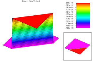
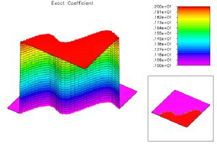
(a)                                            (b)

Figure 1: Pictures (a) and (b) show the two different doping profiles to be reconstructed in the numerical experiments.

For the experiments concerning pointwise measurements of the current density, we assume that only one measurement is available, i.e. $N=1$ in (26).

The first numerical experiment is shown in Figure 2. Here exact data is used for the reconstruction of the p-n junction in Figure 1 (b). The pictures correspond to plots of the iteration error after 5, 10 and 100 steps of the level set method.

The second experiment (see Figure 3) concerns the reconstruction of the p-n junction in Figure 1 (a). In this experiment the data is contaminated with 10% random noise. The pictures correspond to plots of the iteration error after 10, 100 and 400 steps of the level set method.

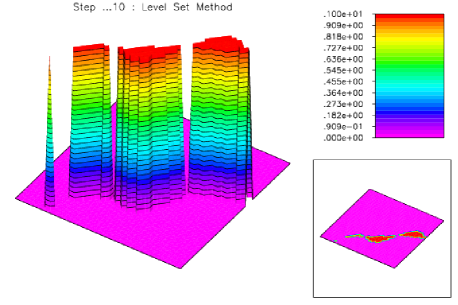
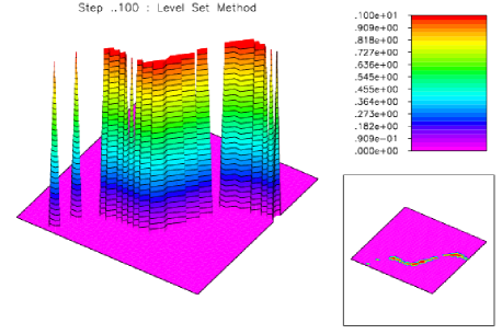
Figure 2: First experiment for the unipolar model with pointwise measurements of the current density: Reconstruction of the p-n junction in Figure 1 (b). Evolution of the iteration error for exact data and one measurement of the DtN map $\Lambda_{\gamma}$ (i.e. $N=1$ in (26)).

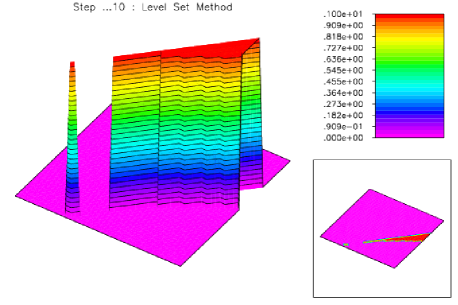
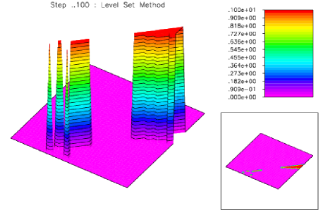
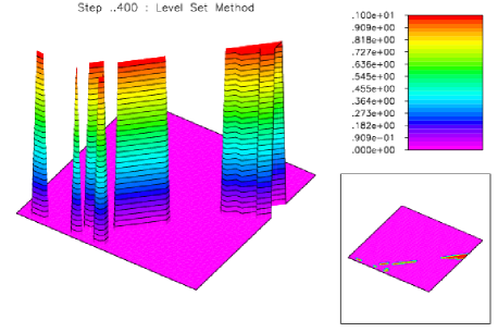
Figure 3: Second experiment for the unipolar model with pointwise measurements of the current density: Reconstruction of the p-n junction in Figure 1 (a). Only one measurement of the DtN map $\Lambda_{\gamma}$ is available (i.e. $N=1$ in (26)). Evolution of the iteration error for the level set method and data contaminated with 10% random noise.

6.2 Stationary linearized unipolar model: current flow measurements through a contact

In what follows we consider the same unipolar model as in Subsection 6.1. Again we shall focus on the identification problem related to (25). However, the coefficient $\gamma$ has to be identified from measurements of the current flow through the contact $\Gamma_{1}$, i.e. from

$$\int_{\Gamma_{1}}\gamma\hat{u}_{\nu}\,ds\,,$$

where $\hat{u}$ solve (25) for prescribed inputs $U\in H^{3/2}(\partial\Omega_{D})$.

An immediate remark is that the amount of available data is much larger in the case of pointwise measurements of the current density than in the case of current flow measurements through a contact. Notice that the inverse doping profile problem in the linearized unipolar model for measurements of the current flow through the contact $\Gamma_{1}$ reduces to the identification of the parameter $\gamma$ in (25) from measurements of the (averaged) DtN map

$$\widetilde{\Lambda}_{\gamma}:\begin{array}[t]{rcl}H^{3/2}(\partial\Omega_{D})&\to&\mathbb{R}\\ U&\mapsto&\int_{\Gamma_{1}}\gamma\,\hat{u}_{\nu}\,ds\end{array}$$

As in the previous subsection, we take into account the restrictions imposed by practical experiments, which lead to the following assumptions:

i) The voltage profile $U\in H^{3/2}(\partial\Omega_{D})$ must satisfy $U|_{\Gamma_{1}}=0$;

ii) The identification of $\gamma$ has to be performed from a finite number of measurements, i.e. from the data

$$\big{\{}(U_{j},\widetilde{\Lambda}_{\gamma}(U_{j}))\big{\}}_{j=1}^{N}\in\big{[}H^{3/2}(\partial\Omega_{D})\times\mathbb{R}\big{]}^{N}.$$ (27)

The subsequent numerical tests were performed using the same iterative method of level set type as in the previous subsection. The domain $\Omega\subset\mathbb{R}^{2}$ as well as the boundary parts $\Gamma_{0}$, $\Gamma_{1}$ and $\partial\Omega_{N}$ are defined as before.

For the experiments concerning current flow measurements through the contact $\Gamma_{1}$, we assume that several measurements are available, i.e. $N>>1$ in (27).

The first numerical experiment is shown in Figure 4. Here exact data is used for the reconstruction of the p-n junction in Figure 1 (a). The picture on the left hand side shows the error for the initial guess of the iterative method. The other two pictures correspond to plots of the iteration error after 50 and 250 steps of the level set method respectively.

The second experiment (see Figure 5) concerns the reconstruction of the p-n junction in Figure 1 (b). The available data is contaminated with 1% random noise. The pictures correspond to plots of the iteration error after 100, 2000 and 3000 steps of the level set method.

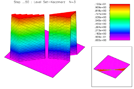
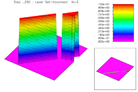
Figure 4: First experiment for the unipolar model with current flow measurements through the contact $\Gamma_{1}$: Reconstruction of the p-n junction in Figure 1 (a). Three measurements of the DtN map $\widetilde{\Lambda}_{\gamma}$ are used in the reconstruction (i.e. $N=3$ in (27)). Evolution of the iteration error for exact data.

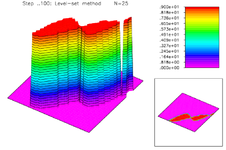
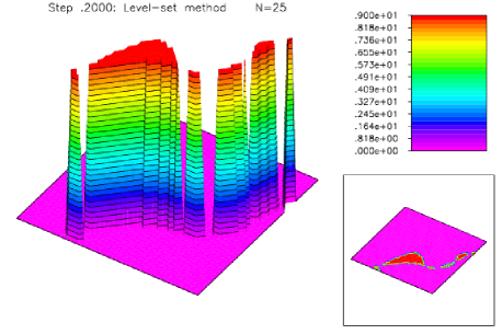
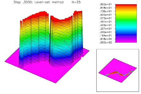
Figure 5: Second experiment for the unipolar model with current flow measurements through the contact $\Gamma_{1}$: Reconstruction of the p-n junction in Figure 1 (b). The data consists of twenty five measurements of the DtN map $\widetilde{\Lambda}_{\gamma}$ (i.e. $N=25$ in (27)). Plots of the iteration error after 100, 2000 and 3000 steps. Data with 1% random noise.

6.3 Stationary linearized bipolar model: pointwise measurements of the current density

In the sequel we consider the bipolar model introduced in Subsection 3.2. As in the unipolar model, it follows from the assumption $Q=0$ that the Poisson equation (7a) and the continuity equations (10a), (10b) decouple. The inverse doping profile problem corresponds to the identification of $C=C(x)$ from pointwise measurements of the total current density $J=J_{n}+J_{p}$, namely

$$(\mu_{n}e^{V_{\rm bi}}\hat{u}_{\nu}-\mu_{p}e^{-V_{\rm bi}}\hat{v}_{\nu})|_{\Gamma_{1}}\mbox{ .}$$

Compare with the Gateaux derivative of the V-C map $\Sigma_{C}$ at the point $U=0$ in (9). Here $(V^{0},\hat{u},\hat{v})$ solve, for each applied voltage $U$, the system (7), (10) (with $h$ substituted by $U$).

As in the unipolar case, we can split the inverse problem in two parts: First we define the function $\gamma(x)\stackrel{{\scriptstyle\mbox{\scriptsize def}}}{{=}}e^{V^{0}(x)}$, $x\in\Omega$, and solve the parameter identification problem

$$\left\{\begin{array}[]{rcl@{\ }l}{\rm div}\,(\mu_{n}\gamma\nabla\hat{u})&=&0&{\rm in}\ \Omega\\ \hat{u}&=&-U(x)&{\rm on}\ \partial\Omega_{D}\\ \nabla\hat{u}\cdot\nu&=&0&{\rm on}\ \partial\Omega_{N}\end{array}\right.\hskip 5.69046pt\left\{\begin{array}[]{rcl@{\ }l}{\rm div}\,(\mu_{p}\gamma^{-1}\nabla\hat{v})&=&0&{\rm in}\ \Omega\\ \hat{v}&=&U(x)&{\rm on}\ \partial\Omega_{D}\\ \nabla\hat{v}\cdot\nu&=&0&{\rm on}\ \partial\Omega_{N}\end{array}\right.$$ (28)

for $\gamma$, from measurements of $(\mu_{n}\gamma\hat{u}_{\nu}-\mu_{p}\gamma^{-1}\hat{v}_{\nu})|_{\Gamma_{1}}$. The second step consists in the determination of $C$ in

$$C(x)\ =\ \gamma(x)-\gamma^{-1}(x)-\lambda^{2}\,\Delta(\ln\gamma(x))\,,\ x\in\Omega\,.$$

Analogous to the unipolar case, the evaluation of $C$ from $\gamma$ can be performed in a stable way. Therefore, we shall focus on the problem of identifying the function parameter $\gamma$ in (28). Notice that the inverse doping profile problem in the linearized bipolar model for pointwise measurements of the current density reduces to the identification of the parameter $\gamma$ in (28) from measurements of the Dirichlet to Neumann (DtN) map

$$\Phi_{\gamma}:\begin{array}[t]{rcl}H^{3/2}(\partial\Omega_{D})&\to&H^{1/2}(\Gamma_{1})\,.\\ U&\mapsto&(\mu_{n}\gamma\hat{u}_{\nu}-\mu_{p}\gamma^{-1}\hat{v}_{\nu})|_{\Gamma_{1}}\end{array}$$

As before we take into account the restrictions imposed by the practical experiments, from what follows:

i) The voltage profiles $U\in H^{3/2}(\partial\Omega_{D})$ must satisfy $U|_{\Gamma_{1}}=0$;

ii) The identification of $\gamma$ has to be performed from a finite number of measurements, i.e. from the data

$$\big{\{}(U_{j},\Phi_{\gamma}(U_{j}))\big{\}}_{j=1}^{N}\in\big{[}H^{3/2}(\partial\Omega_{D})\times H^{1/2}(\Gamma_{1})\big{]}^{N}.$$ (29)

In Figure 6 we present a numerical experiment for the bipolar model with pointwise measurements of the current density. Here exact data is used for the reconstruction of the p-n junction in Figure 1 (b). The pictures show plots of the iteration error after 1, 10 and 100 steps of the level set method respectively.

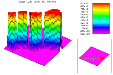
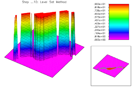
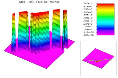
Figure 6: Experiment for the bipolar model with pointwise measurements of the current density: Reconstruction of the p-n junction in Figure 1 (b). Evolution of the iteration error for exact data and one measurement of the DtN map $\Phi_{\gamma}$ (i.e. $N=1$ in (29)).

6.4 Remarks and conclusions

The best numerical results are obtained for the experiments concerning the linearized unipolar case with pointwise measurements of the current density. In this model, a single measurement of the DtN map $\Lambda_{\gamma}$, i.e. $N=1$ in (26), contains enough information about the structure of the doping profile and suffices to obtain a very precise reconstruction of the p-n junction. This is the case even for highly oscillating p-n junctions as shown in Figure 2 and also in the presence of noise (see Figure 3). We observed that the iteration is extremely robust with respect to the choice of the initial guess and also with respect to high levels of noise.

Concerning the linearized unipolar model with current flow measurements through the contact $\Gamma_{1}$, our experiments show that the (averaged) DtN map $\widetilde{\Lambda}_{\gamma}$, furnishes much less information about the solution structure than the map $\Lambda_{\gamma}$. Depending on the complexity of the p-n junction, more measurements of $\widetilde{\Lambda}_{\gamma}$ may be needed in order to obtain an acceptable reconstruction. The experiments show that a single measurement ($N=1$ in (27)) is not enough to identify the doping profile in Figure 1 (a). Moreover, although three measurements have shown to be enough to reconstruct this p-n junction (see Figure 4), this is not the case for the p-n junction in Figure 1 (b). For this second and more complex junction, we first obtained more accurate reconstructions with $N=19$ in (27). The quality of the reconstruction obtained for $N=25$ is already very high (see Figure 5) and does not qualitatively improve for larger values of $N$ (we experimented up to $N=49$).

It is worth noticing that the number of iterative steps required by the level set algorithm to reach the stopping criteria for the inverse problem related to the map $\widetilde{\Lambda}_{\gamma}$ is greater than that for the operator $\Lambda_{\gamma}$. This is again explained by the fact that the range of $\widetilde{\Lambda}_{\gamma}$ lies in $\mathbb{R}$, while the range of $\Lambda_{\gamma}$ lies in $H^{1/2}(\Gamma_{1})$.

Concerning the experiments for the linearized bipolar model with pointwise measurements of the current density, the quality of the results is comparable to those in Subsection 6.1 and, as in that subsection, a single measurement of the operator $\Phi_{\gamma}$ ($N=1$ in (29)) suffices to precisely reconstruct the p-n junction. We observed, however, that convergence of the iterative method is more sensitive to the choice of the initial condition than in Subsection 6.1.

Appendix

Properties of silicon at room temperature

Parameter	Typical value
$\epsilon_{s}$	$11.9\ \epsilon_{0}$
$\mu_{n}$	$\approx 1500\ {\rm cm}^{2}\ {\rm V}^{-1}\ {\rm s}^{-1}$
$\mu_{p}$	$\approx 450\ {\rm cm}^{2}\ {\rm V}^{-1}\ {\rm s}^{-1}$
$C_{n}$	$2.8\times 10^{-31}\ {\rm cm}^{6}{\rm/s}$
$C_{p}$	$9.9\times 10^{-32}\ {\rm cm}^{6}{\rm/s}$
$\tau_{n}$	$10^{-6}\,{\rm s}$
$\tau_{p}$	$10^{-5}\,{\rm s}$

Table 1: Typical values of main the constants in the model.

Relevant physical constants:

• Permittivity of vacuum: $\epsilon_{0}=8.85\times 10^{-14}{\rm As\,V}^{-1}\,{\rm cm}^{-1}$;

• Elementary charge: $q=1.6\times 10^{-19}{\rm As}$.

References

- APL (05) Astala, K., Päivärinta, L., Lassas, M.: Calderón’s inverse problem for anisotropic conductivity in the plane. Comm. Partial Differential Equations 30, 207–224 (2005)
- BL (05) Baumeister, J. and Leitão, A.: Topics in inverse problems. Mathematical Publications of IMPA. ISBN: 85-244-0224-5 25th Brazilian Mathematics Colloquium. Rio de Janeiro, Brazil. (2005)
- Bor (02) Borcea, L.: Electrical impedance tomography. Inverse Problems 18, R99–R136 (2002)
- BU (02) Bukhgeim, A., Uhlmann, G.: Recovering a potential from partial Cauchy data. Comm. Partial Differential Equations 27, 653–668 (2002)
- BELM (04) Burger, M., Engl, H.W., Leitão, A., Markowich, P.A.: On inverse problems for semiconductor equations. Milan Journal of Mathematics 72, 273–314 (2004)
- BEMP (01) Burger, M., Engl, H.W., Markowich, P.A., Pietra, P.: Identification of doping profiles in semiconductor devices. Inverse Problems 17, 1765–1795 (2001)
- BEM (02) Burger, M., Engl, H.W., P. Markowich, P.A.: Inverse doping problems for semiconductor devices. In: Chan, T.F. et al (eds) Recent Progress in Computational and Applied PDEs. Kluwer/Plenum, New York, 39–53 (2002)
- BF (91) Busenberg, S., Fang, W.: Identification of semiconductor contact resistivity. Quart. Appl. Math. 49, 639–649 (1991)
- BFI (93) Busenberg, S., Fang, W., Ito, K.: Modeling and analysis of laser-beam-inducted current images in semiconductors. SIAM J. Appl. Math. 53, 187–204 (1993)
- Bur (01) Burger, M.: A level set method for inverse problems. Inverse Problems 17, 1327–1355 (2001)
- DES (98) Deuflhard, P., Engl, H.W., O. Scherzer, O.: A convergence analysis of iterative methods for the solution of nonlinear ill-posed problems under affinely invariant conditions. Inverse Problems 14, 1081–1106 (1998)
- EHN (96) Engl, H.W., Hanke, M., Neubauer, A.: Regularization of Inverse Problems. Kluwer Academic Publishers, Dordrecht (1996)
- EKN (89) Engl, H.W., Kunisch, K., Neubauer, A.: Convergence rates for Tikhonov regularization of nonlinear ill-posed problems. Inverse Problems 5, 523–540 (1989)
- ES (00) Engl, H.W., Scherzer, O.: Convergence rates results for iterative methods for solving nonlinear ill-posed problems. In: Colton, D. et al (eds), Surveys on solution methods for inverse problems. Springer, Vienna, 7–34 (2000)
- FC (92) Fang, W., Cumberbatch, E.: Inverse problems for metal oxide semiconductor field-effect transistor contact resistivity. SIAM J. Appl. Math. 52, 699–709 (1992)
- FI (92) Fang, W., Ito, K.: Identifiability of semiconductor defects from LBIC images. SIAM J. Appl. Math. 52, 1611–1626 (1992)
- FI (94) Fang, W., Ito, K.: Reconstruction of semiconductor doping profile from laser-beam-induced current image. SIAM J. Appl. Math. 54, 1067–1082 (1994)
- FIR (02) Fang, W., Ito, K., Redfern, D.A.: Parameter identification for semiconductor diodes by LBIC imaging. SIAM J. Appl. Math. 62, 2149–2174 (2002)
- FSL (05) Frühauf, F., Scherzer, O., Leitão, A.: Analysis of regularization methods for the solution of ill–posed problems involving discontinuous operators. SIAM J Numerical Analysis 43, 767–786 (2005)
- Gaj (85) Gajewski, H.: On existence, uniqueness and asymptotic behavior of solutions of the basic equations for carrier transport in semiconductors. Z. Angew. Math. Mech. 65, 101–108 (1985)
- GV (89) Golub, G. H. & C. F. Van Loan (1989) Matrix computations (Second ed.) Johns Hopkins University Press, Baltimore, MD.
- Gri (85) Grisvard, P.: Elliptic Problems in Nonsmooth Domains. Pittman Publishing, London, (1985)
- HNS (95) Hanke, M., Neubauer, A., Scherzer, O.: A convergence analysis of the Landweber iteration for nonlinear ill-posed problems. Numer. Math. 72, 21–37 (1995)
- Isa (98) Isakov, V.: Inverse problems for partial differential equations. Applied Mathematical Sciences, Springer, New York (1998)
- KS (02) Kowar, R., Scherzer, O.: Convergence analysis of a Landweber-Kaczmarz method for solving nonlinear ill-posed problems. In Kabanikhin, S.I. et al (eds), Ill-Posed and Inverse Problems. VSP, Boston, 253–270 (2002)
- LS (03) Leitão, A., Scherzer, O.: On the relation between constraint regularization, level sets, and shape optimization. Inverse Problems 19, L1–L11 (2003)
- LMZ (05) Leitão, A., Markowich, P.A., Zubelli, J.P.: On inverse doping profile problems for the voltage-current map. Inverse Problems, submitted (2005)
- Mar (86) Markowich, P.A.: The Stationary Semiconductor Device Equations. Springer, Vienna (1986)
- MRS (90) P.A. Markowich, C.A. Ringhofer, C. Schmeiser, Semiconductor Equations. Springer, Vienna (1990)
- Nac (96) Nachman, A.I.: Global uniqueness for a two-dimensional inverse boundary value problem. Ann. of Math. 143, 71–96 (1996)
- OS (88) Osher, S. and Sethian, J.: Fronts propagation with curvature dependent speed: Algorithms based on Hamilton-Jacobi formulation. J. of Computational Physics., 56, 12–49 (1988)
- San (95) Santosa, F.: A level-set approach for inverse problems involving obstacles, ESAIM Contrôle Optim. Calc. Var., 1, 17–33 (1995/96)
- Sch (91) Scherzer, O.: Tikhonov regularization of nonlinear ill-posed problems with applications to parameter identification in partial differential equations. PhD Thesis Johannes-Kepler-Universität, Linz (1991)
- Sel (84) Selberherr, S.: Analysis and Simulation of Semiconductor Devices. Springer, New York (1984)
- vRo (50) van Roosbroeck, W.R.: Theory of flow of electrons and holes in germanium and other semiconductors. Bell Syst. Tech. J. 29, 560–607 (1950)
- TA (77) Tikhonov, A.N., Arsenin, V.Y.: Solutions of Ill-posed Problems. John Wiley & Sons, New York (1977)