Nucleon Momentum Fraction, Helicity and Transversity from $2+1$-flavor Lattice QCD

Abstract

High statistics results for the isovector momentum fraction, $\langle x\rangle_{u-d}$, helicity moment, $\langle x\rangle_{\Delta u-\Delta d}$, and the transversity moment, $\langle x\rangle_{\delta u-\delta d}$, of the nucleon are presented using seven ensembles of gauge configurations generated by the JLab/W&M/LANL/MIT collaborations using $2+1$-flavors of dynamical Wilson-clover quarks. Attention is given to understanding and controlling the contributions of excited states. The final result is obtained using a simultaneous fit in the lattice spacing $a$, pion mass $M_{\pi}$ and the finite volume parameter $M_{\pi}L$ keeping leading order corrections. The data show no significant dependence on the lattice spacing and some evidence for finite-volume corrections. The main variation is with $M_{\pi}$, whose magnitude depends on the mass gap of the first excited state used in the analysis. Our final results, in the $\overline{\rm MS}$ scheme at 2 GeV, are $\langle x\rangle_{u-d}=0.160(16)(20)$, $\langle x\rangle_{\Delta u-\Delta d}=0.192(13)(20)$ and $\langle x\rangle_{\delta u-\delta d}=0.215(17)(20)$, where the first error is the overall analysis uncertainty assuming excited-state contributions have been removed, and the second is an additional systematic uncertainty due to possible residual excited-state contributions. These results are consistent with other recent lattice calculations and phenomenological global fit values.

I Introduction

Steady progress in both experiment and theory is providing an increasingly detailed description of the hadron structure in terms of quarks and gluons. The distributions of quarks and gluons within nucleons are being probed in experiments at the Relativistic Heavy Ion Collider (RHIC) at BNL Djawotho (2013); Adare et al. (2014), Jefferson Lab Dudek et al. (2012) and the Large Hadron Collider at CERN. Experiments at the planned electron-ion collider Accardi et al. (2016a) will significantly extend the range of Bjorken $x$ and $Q^{2}$ and further improve our understanding. From these data, and using higher order calculations of electroweak and strong corrections, the phenomenological analyses of experimental data (global fits) are providing parton distribution functions (PDFs) Brock et al. (1995); Ji et al. (2020), transverse momentum dependent PDFs (TMDs) Yoon et al. (2017a), and generalized parton distributions (GPDs) Diehl (2003). These distributions are not measured directly in experiments Cichy and Constantinou (2019); Karthik (2019), necessitating phenomenological analyses that have involved different theoretical inputs.

Lattice QCD calculations are beginning to provide such input, and a review of the cross-fertilization between the two efforts has been presented in Refs. Lin et al. (2018); Constantinou et al. (2020). With increasing computing power and advances in algorithms, the precision of lattice QCD calculations has increased significantly and there now exist many quantities for which there is good agreement with experimental results, and for some, the lattice results are the most precise as reviewed in the recent Flavor Averaging Group (FLAG) 2019 report Aoki et al. (2020).

In this work, we present high-statistics lattice data for the isovector momentum fraction, and the helicity and transversity moments, whose calculation is now reaching precision comparable to that for nucleon charges, which are the zeroth moments of the distributions and obtained from the matrix elements of local quark bilinear operators Gupta et al. (2018); Aoki et al. (2020).

Calculations for the three first moments, $\langle x\rangle_{u-d}$, $\langle x\rangle_{\Delta u-\Delta d}$ and $\langle x\rangle_{\delta u-\delta d}$, have been done on seven ensembles generated using 2+1-flavors of Wilson-clover quarks by the JLab/W&M/LANL/MIT collaborations Edwards et al. (2016). The data at three values of lattice spacings $a$, two values of the pion mass, $M_{\pi}\approx 170$ and $\approx 270$ MeV, and on a range of large volumes, characterized by $M_{\pi}L$, allow us to carry out a simultaneous fit in these three variables to address the associated systematic uncertainties. In the analysis of the two- and three-point correlation functions from each ensemble, we carry out a detailed investigation of the dependence of the results on the spectra of possible, $a\ priori$ unresolved, excited states included in the fits to remove excited-state contamination (ESC). Concretely, the full analysis is carried out using three strategies to estimate the mass gap of the first excited state from the two- and three-point correlation functions, and we use the spread in the results to assign a second systematic uncertainty to account for possible remaining contributions from excited-states.

Our final results, given in Eq. (78), are $\langle x\rangle_{u-d}=0.160(16)(20)$, $\langle x\rangle_{\Delta u-\Delta d}=0.192(13)(20)$ and $\langle x\rangle_{\delta u-\delta d}=0.215(17)(20)$ in the $\overline{\rm MS}$ scheme at 2 GeV. These estimates are in good agreement with other lattice and phenomenological global fit results as discussed in Sec. VI. The most extensive and precise results from global fits are for the unpolarized moments of the nucleons, the momentum fraction $\langle x\rangle_{q}$, while those for the helicity fraction, the polarized moment $\langle x\rangle_{\Delta q}$, have a large spread and our lattice results are consistent with the smaller error global fit values at the lower end. Lattice QCD results for the transversity $\langle x\rangle_{\delta q}$ are a prediction due to lack of sufficient experimental data Lin et al. (2018); Constantinou et al. (2020).

The paper is organized as follows: In Sec. II, we briefly summarize the lattice parameters and methodology. The definitions of moments and operators investigated are given in Sec. III. The two- and three-point functions calculated, and their connection to the moments, are specified in Sec. IV. The analysis of excited state contributions and the extraction of the ground state matrix elements is presented in Sec. V. Results for the moments after the chiral-continuum-finite-volume (CCFV) extrapolation are given in Sec. VI, and compared with other lattice calculations and global fit values. We end with conclusions in Sec. VII. The data and fits used to remove excited-state contamination are shown in Appendix A and the calculation of the renormalization factors, $Z_{VD,AD,TD}$, for the three operators is discussed in Appendix B.

II Lattice Methodology

This work follows closely the methodology described in Ref. Mondal et al. (2020), with two major differences. The first is the calculation here uses 2+1-flavors of Wilson-clover fermions in a clover-on-clover unitary formulation of lattice QCD, whereas the clover-on-HISQ formulation was used in Ref. Mondal et al. (2020). The clover action includes one iteration of stout smearing with weight $\rho=0.125$ for the staples Morningstar and Peardon (2004). The tadpole corrected tree-level Sheikholeslami-Wohlert coefficient $c_{SW}=1/u_{0}$ Sheikholeslami and Wohlert (1985), where $u_{0}$ is the fourth root of the plaquette expectation value, is very close to the nonperturbative value determined, a posteriori, using the Schrödinger functional method Luscher et al. (1997), a consequence of the stout smearing. The update of configurations was carried out using the rational hybrid Monte Carlo (RHMC) algorithm Duane et al. (1987) as described in Ref. Yoon et al. (2017b).

The parameters of the seven clover ensembles generated by the JLab/W&M/LANL/MIT collaborations Edwards et al. (2016) and used in the analysis are summarized in Table 1. The range of lattice spacings covered is $0.071\leq a\leq 0.127$ fm and of lattice size is $3.7\leq M_{\pi}L\leq 6.2$. So far simulations have been carried out at two pion masses, $M_{\pi}\approx 270$ and 170 MeV. These seven data points allow us to perform chiral-continuum-finite-volume fits to obtain physical results.

The second improvement is higher statistics data that lead to a more robust analysis of three strategies for evaluating ESC. Table 1 also gives the number of configurations, the source-sink separations $\tau$, high precision (HP) and low precision (LP) measurements made to cost-effectively increase statistics using the bias-corrected truncated-solver method Bali et al. (2010); Blum et al. (2013).

The parameters used to construct the Gaussian smeared sources Güsken et al. (1988); Yoon et al. (2016); Gupta et al. (2018); Mondal et al. (2020), are given in Table 2. To construct the smeared source, the gauge links were first smoothened using twenty hits of the stout algorithm with $\rho=0.08$ and including only the spatial staples. The root-mean-square size of the Gaussian smearing, $\sqrt{\int dr\,r^{4}S^{\dagger}S/\int dr\,r^{2}S^{\dagger}S}$ with $S(r)$ the value of the smeared source at radial distance $r$, was adjusted to be between 0.72—0.76 fm to reduce ESC. The quark propagators from these smeared sources were generated by inverting the Dirac operator (same as what was used to generate the lattices) using the multigrid algorithm Babich et al. (2010); Clark et al. (2010, 2016). These propagators are then used to construct the two- and three-point correlation functions.

Ensemble	$a$	$M_{\pi}$	$L^{3}\times T$	$M_{\pi}L$	$\tau/a$	$N_{conf}$	$N_{HP}$	$N_{LP}$
ID	(fm)	(MeV)
$a127m285$	$0.127(2)$	$285(3)$	$32^{3}\times 96$	$5.85$	$\{8,10,12,14\}$	$2001$	$8,004$	$256,128$
$a094m270$	$0.094(1)$	$270(3)$	$32^{3}\times 64$	$4.11$	$\{10,12,14,16\}$	$1464$	$4,392$	$140,544$
$a094m270L$	$0.094(1)$	$269(3)$	$48^{3}\times 128$	$6.16$	$\{8,10,12,14,16,18\}$	$4501$	$18,004$	$576,128$
$a091m170$	$0.091(1)$	$169(2)$	$48^{3}\times 96$	$3.75$	$\{8,10,12,14,16\}$	$4015$	$16,060$	$513,920$
$a091m170L$	$0.091(1)$	$169(2)$	$64^{3}\times 128$	$5.08$	$\{8,10,12,14,16\}$	$1533$	$7,665$	$245,280$
$a073m270$	$0.0728(8)$	$272(3)$	$48^{3}\times 128$	$4.82$	$\{11,13,15,17,19\}$	$4477$	$17,908$	$573,056$
$a071m170$	$0.0707(8)$	$167(2)$	$72^{3}\times 192$	$4.26$	$\{13,15,17,19,21\}$	$1500$	$9,000$	$144,000$

Table 1: Lattice parameters of the 2+1-flavor clover ensembles generated by the JLab/W&M/LANL/MIT collaboration and analyzed in this study. We specify the lattice spacing $a$, pion mass $M_{\pi}$, lattice size $L^{3}\times T$, the values of source-sink separation $\tau$ simulated, the number of configurations analyzed, and the total number of high precision (HP) and low precision (LP) measurements made.

ID	$m_{l}$	$c_{\text{SW}}$	Smearing	RMS
			Parameters	smearing
			$\{\sigma,N_{\text{KG}}\}$	radius
$a127m285$	$-0.2850$	1.24931	{5, 50}	5.79(1)
$a094m270$	$-0.2390$	1.20537	{7, 91}	7.72(3)
$a094m270L$	$-0.2390$	1.20537	{7, 91}	7.76(4)
$a091m170$	$-0.2416$	1.20537	{7, 91}	7.64(3)
$a091m170L$	$-0.2416$	1.20537	{7, 91}	7.76(4)
$a073m270$	$-0.2070$	1.17008	{9, 150}	9.84(1)
$a071m170$	$-0.2091$	1.17008	{10, 185}	10.71(2)

Table 2: The parameters used in the calculation of the clover propagators. The hopping parameter for the light quarks, $\kappa_{l}$, in the clover action is given by $2\kappa_{l}=1/(m_{l}+4)$. $c_{\rm SW}$ is the Sheikholeslami-Wohlert improvement coefficient in the clover action. The parameters used to construct Gaussian smeared sources Gusken et al. (1989), $\{\sigma,N_{\text{KG}}\}$ in the Chroma convention Edwards and Joo (2005), are given in the fourth column where $N_{\text{KG}}$ is the number of applications of the Klein-Gordon operator and $\sigma$ controls the width of the smearing. The resulting root-mean-square radius of the smearing in lattice units, defined as $\sqrt{\int dr\,r^{4}S^{\dagger}S/\int dr\,r^{2}S^{\dagger}S}$ with $S(r)$ the value of the smeared source at radial distance $r$, is given in the last column.

III Moments and Matrix elements

The first moments of spin independent (or unpolarized), $q=q_{\uparrow}+q_{\downarrow}$, helicity (or polarized), $\Delta q=q_{\uparrow}-q_{\downarrow}$, and transversity, $\delta q=q_{\top}+q_{\perp}$ distributions, are defined as

$$\langle x\rangle_{q} = \int_{0}^{1}\leavevmode\nobreak\ x\leavevmode\nobreak\ [q(x)+\overline{q}(x)]\leavevmode\nobreak\ dx\,,$$ (1)

$$\langle x\rangle_{\Delta q} = \int_{0}^{1}\leavevmode\nobreak\ x\leavevmode\nobreak\ [\Delta q(x)+\Delta\overline{q}(x)]\leavevmode\nobreak\ dx\,,$$ (2)

$$\langle x\rangle_{\delta q} = \int_{0}^{1}\leavevmode\nobreak\ x\leavevmode\nobreak\ [\delta q(x)+\delta\overline{q}(x)]\leavevmode\nobreak\ dx\,,$$ (3)

where $q_{\uparrow(\downarrow)}$ corresponds to quarks with helicity aligned (anti-aligned) with that of a longitudinally polarized target, and $q_{\top(\perp)}$ corresponds to quarks with spin aligned (anti-aligned) with that of a transversely polarized target.

These moments, at leading twist, are extracted from the forward matrix elements of one-derivative vector, axial-vector and tensor operators within ground state nucleons at rest. The complete set of the relevant twist two operators are

$${\cal O}^{\mu\nu}_{V^{a}} = \overline{q}\gamma^{\{\mu}\mathchoice{\vbox{\halign{#\cr\leftrightarrowfill@{\scriptstyle}\crcr\nointerlineskip\cr$\hfil\displaystyle D\hfil$\crcr}}}{\vbox{\halign{#\cr\leftrightarrowfill@{\scriptstyle}\crcr\nointerlineskip\cr$\hfil\textstyle D\hfil$\crcr}}}{\vbox{\halign{#\cr\leftrightarrowfill@{\scriptscriptstyle}\crcr\nointerlineskip\cr$\hfil\scriptstyle D\hfil$\crcr}}}{\vbox{\halign{#\cr\leftrightarrowfill@{\scriptscriptstyle}\crcr\nointerlineskip\cr$\hfil\scriptscriptstyle D\hfil$\crcr}}}^{\nu\}}\tau^{a}q\,,$$ (12)

$${\cal O}^{\mu\nu}_{A^{a}} = \overline{q}\gamma^{\{\mu}\mathchoice{\vbox{\halign{#\cr\leftrightarrowfill@{\scriptstyle}\crcr\nointerlineskip\cr$\hfil\displaystyle D\hfil$\crcr}}}{\vbox{\halign{#\cr\leftrightarrowfill@{\scriptstyle}\crcr\nointerlineskip\cr$\hfil\textstyle D\hfil$\crcr}}}{\vbox{\halign{#\cr\leftrightarrowfill@{\scriptscriptstyle}\crcr\nointerlineskip\cr$\hfil\scriptstyle D\hfil$\crcr}}}{\vbox{\halign{#\cr\leftrightarrowfill@{\scriptscriptstyle}\crcr\nointerlineskip\cr$\hfil\scriptscriptstyle D\hfil$\crcr}}}^{\nu\}}\gamma^{5}\tau^{a}q\,,$$ (21)

$${\cal O}^{\mu\nu\rho}_{T^{a}} = \overline{q}\sigma^{[\mu\{\nu]}\mathchoice{\vbox{\halign{#\cr\leftrightarrowfill@{\scriptstyle}\crcr\nointerlineskip\cr$\hfil\displaystyle D\hfil$\crcr}}}{\vbox{\halign{#\cr\leftrightarrowfill@{\scriptstyle}\crcr\nointerlineskip\cr$\hfil\textstyle D\hfil$\crcr}}}{\vbox{\halign{#\cr\leftrightarrowfill@{\scriptscriptstyle}\crcr\nointerlineskip\cr$\hfil\scriptstyle D\hfil$\crcr}}}{\vbox{\halign{#\cr\leftrightarrowfill@{\scriptscriptstyle}\crcr\nointerlineskip\cr$\hfil\scriptscriptstyle D\hfil$\crcr}}}^{\rho\}}\tau^{a}q\,,$$ (30)

where $q=\{u,d\}$ is the isodoublet of light quarks and $\sigma^{\mu\nu}=(\gamma^{\mu}\gamma^{\nu}-\gamma^{\nu}\gamma^{\mu})/2$. The derivative $\mathchoice{\vbox{\halign{#\cr\leftrightarrowfill@{\scriptstyle}\crcr\nointerlineskip\cr$\hfil\displaystyle D\hfil$\crcr}}}{\vbox{\halign{#\cr\leftrightarrowfill@{\scriptstyle}\crcr\nointerlineskip\cr$\hfil\textstyle D\hfil$\crcr}}}{\vbox{\halign{#\cr\leftrightarrowfill@{\scriptscriptstyle}\crcr\nointerlineskip\cr$\hfil\scriptstyle D\hfil$\crcr}}}{\vbox{\halign{#\cr\leftrightarrowfill@{\scriptscriptstyle}\crcr\nointerlineskip\cr$\hfil\scriptscriptstyle D\hfil$\crcr}}}^{\nu}\equiv\frac{1}{2}(\overrightarrow{D}^{\nu}-\overleftarrow{D}^{\nu})$ consists of four terms defined in Ref. Mondal et al. (2020). Lorentz indices within $\{\leavevmode\nobreak\ \}$ in Eq. (30) are symmetrized and within $[\,]$ are antisymmetrized. It is also implicit that, where relevant, the traceless part of the above operators is taken. Their renormalization is carried out nonperturbatively in the regularization independent RI^′-MOM scheme as discussed in Appendix B. A more detailed discussion of these twist-2 operators and their renormalization can be found in Refs. Gockeler et al. (1996) and Harris et al. (2019).

In our setup to calculate the isovector moments, we work with $\tau^{a}=\tau^{3}$ and fix the spin of the nucleon state to be in the “3” direction. With these choices, the explicit operators calculated are

$${\cal O}^{44}_{V^{3}} = \overline{q}(\gamma^{4}\mathchoice{\vbox{\halign{#\cr\leftrightarrowfill@{\scriptstyle}\crcr\nointerlineskip\cr$\hfil\displaystyle D\hfil$\crcr}}}{\vbox{\halign{#\cr\leftrightarrowfill@{\scriptstyle}\crcr\nointerlineskip\cr$\hfil\textstyle D\hfil$\crcr}}}{\vbox{\halign{#\cr\leftrightarrowfill@{\scriptscriptstyle}\crcr\nointerlineskip\cr$\hfil\scriptstyle D\hfil$\crcr}}}{\vbox{\halign{#\cr\leftrightarrowfill@{\scriptscriptstyle}\crcr\nointerlineskip\cr$\hfil\scriptscriptstyle D\hfil$\crcr}}}^{4}-\frac{1}{3}{\bm{\gamma}}\cdot\mathchoice{\vbox{\halign{#\cr\leftrightarrowfill@{\scriptstyle}\crcr\nointerlineskip\cr$\hfil\displaystyle\bf D\hfil$\crcr}}}{\vbox{\halign{#\cr\leftrightarrowfill@{\scriptstyle}\crcr\nointerlineskip\cr$\hfil\textstyle\bf D\hfil$\crcr}}}{\vbox{\halign{#\cr\leftrightarrowfill@{\scriptscriptstyle}\crcr\nointerlineskip\cr$\hfil\scriptstyle\bf D\hfil$\crcr}}}{\vbox{\halign{#\cr\leftrightarrowfill@{\scriptscriptstyle}\crcr\nointerlineskip\cr$\hfil\scriptscriptstyle\bf D\hfil$\crcr}}})\tau^{3}q\,,$$ (47)

$${\cal O}^{34}_{A^{3}} = \overline{q}\gamma^{\{3}\mathchoice{\vbox{\halign{#\cr\leftrightarrowfill@{\scriptstyle}\crcr\nointerlineskip\cr$\hfil\displaystyle D\hfil$\crcr}}}{\vbox{\halign{#\cr\leftrightarrowfill@{\scriptstyle}\crcr\nointerlineskip\cr$\hfil\textstyle D\hfil$\crcr}}}{\vbox{\halign{#\cr\leftrightarrowfill@{\scriptscriptstyle}\crcr\nointerlineskip\cr$\hfil\scriptstyle D\hfil$\crcr}}}{\vbox{\halign{#\cr\leftrightarrowfill@{\scriptscriptstyle}\crcr\nointerlineskip\cr$\hfil\scriptscriptstyle D\hfil$\crcr}}}^{4\}}\gamma^{5}\tau^{3}q\,,$$ (56)

$${\cal O}^{124}_{T^{3}} = \overline{q}\sigma^{[1\{2]}\mathchoice{\vbox{\halign{#\cr\leftrightarrowfill@{\scriptstyle}\crcr\nointerlineskip\cr$\hfil\displaystyle D\hfil$\crcr}}}{\vbox{\halign{#\cr\leftrightarrowfill@{\scriptstyle}\crcr\nointerlineskip\cr$\hfil\textstyle D\hfil$\crcr}}}{\vbox{\halign{#\cr\leftrightarrowfill@{\scriptscriptstyle}\crcr\nointerlineskip\cr$\hfil\scriptstyle D\hfil$\crcr}}}{\vbox{\halign{#\cr\leftrightarrowfill@{\scriptscriptstyle}\crcr\nointerlineskip\cr$\hfil\scriptscriptstyle D\hfil$\crcr}}}^{4\}}\tau^{3}q\,.$$ (65)

The forward matrix elements ($ME$) of these operators within the ground state of the nucleon with mass $M_{N}$ are related to the moments as follows:

$$\langle 0|{\cal O}^{44}_{V^{3}}|0\rangle = -M_{N}\,\langle x\rangle_{u-d}\,,$$ (66)

$$\langle 0|{\cal O}^{34}_{A^{3}}|0\rangle = -\frac{iM_{N}}{2}\,\langle x\rangle_{\Delta u-\Delta d}\,,$$ (67)

$$\langle 0|{\cal O}^{124}_{T^{3}}|0\rangle = -\frac{iM_{N}}{2}\,\langle x\rangle_{\delta u-\delta d}\,.$$ (68)

The moments are, by construction, dimensionless.

IV Correlation functions and Moments

To construct the two- and three-point correlation functions needed to calculate the matrix elements, the interpolating operator ${\mathcal{N}}$ used to create/annihilate the nucleon state is

$${\mathcal{N}}=\epsilon^{abc}\Big{[}q_{1}^{aT}(x)C\gamma^{5}\frac{(1\pm\gamma_{4})}{2}q_{2}^{b}(x)\Big{]}q^{c}_{1}(x)\,,$$ (69)

where $\{a,b,c\}$ are color indices, $q_{1},q_{2}\in\{u,d\}$ and $C=\gamma_{4}\gamma_{2}$ is the charge conjugation matrix in our convention. The nonrelativistic projection $(1\pm\gamma_{4})/2$ is inserted to improve the signal, with the plus and minus signs applied to the forward and backward propagation in Euclidean time, respectively Gockeler et al. (1996). At zero momentum, this operator couples only to the spin-$\frac{1}{2}$ states. The zero momentum two-point and three-point nucleon correlation functions are defined as

$$\bm{C}^{\rm 2pt}_{\alpha\beta}(\tau) =\sum_{\bm{x}}\langle 0|{\mathcal{N}}_{\alpha}(\tau,{\bm{x}})\overline{{\mathcal{N}}}_{\beta}(0,{\bm{0}})|0\rangle$$ (70)

$$\bm{C}^{\rm 3pt}_{\mathcal{O},\alpha\beta}(\tau,t) =\sum_{{\bm{x}}^{\prime},{\bm{x}}}\langle 0|{\mathcal{N}}_{\alpha}(\tau,{\bm{x}}){\cal O}(t,{\bm{x}}^{\prime})\overline{{\mathcal{N}}}_{\beta}(0,{\bm{0}})|0\rangle$$ (71)

where $\alpha$, $\beta$ are spin indices. The source is placed at time slice 0, the sink is at $\tau$ and the one-derivative operators, defined in Sec. III, are inserted at time slice $t$. Data have been accumulated for the values of $\tau$ specified in Table 1, and for each $\tau$ for all intermediate times $0<t<\tau$.

To isolate the various contributions, projected $2$- and $3$-point functions are constructed as

$$C^{\rm 2pt} = {\rm Tr}\big{(}{\cal P}_{\rm 2pt}\bm{C}^{\rm 2pt}\big{)}$$ (72)

$$C_{\mathcal{O}}^{\rm 3pt} = {\rm Tr}\big{(}{\cal P}_{\rm 3pt}\bm{C}^{\rm 3pt}_{\mathcal{O}}\big{)}\,.$$ (73)

The projector ${\cal P}_{\rm 2pt}=\frac{1}{2}\,(1+\gamma_{4})$ in the nucleon correlator gives the positive parity contribution for the nucleon propagating in the forward direction. For the connected $3$-point contributions ${\cal P}_{\rm 3pt}=\frac{1}{2}(1+\gamma_{4})(1+i\gamma^{5}\gamma^{3})$ is used. With these spin projections, the three moments are obtained using Eqs. 66, 67 and 68.

To display the data, we construct the ratios

$$R_{\mathcal{O}}(\tau;t)=C_{\mathcal{O}}^{3\text{pt}}(\tau;t)/C^{2\text{pt}}(\tau)$$ (74)

that give the ground state matrix element in the limits $t\to\infty$ and $(\tau-t)\to\infty$. These ratios are shown in Figs. 5–10 in Appendix A. We re-emphasize that the ground state matrix element $\langle 0\lvert\mathcal{O}\rvert 0\rangle$ used in the analysis is obtained from fits to $C_{\mathcal{O}}^{3\text{pt}}(\tau;t)$ with input of spectral quantities from $C^{2\text{pt}}(\tau)$. These fits are carried out within a single-elimination jackknife process, which is used to get both the central values and the errors.

Ensemble	$aM_{N}^{\{4\}}$	$aM_{N}^{\{4^{N\pi}\}}$	$a\Delta M_{1}^{\{2\}}$	$a\Delta M_{1}^{\{4\}}$	$a\Delta M_{1}^{\{4^{N\pi}\}}$	$a\Delta M_{1}^{\{2^{\rm free}\}}$	$a\Delta M_{1}^{\{2^{\rm free}\}}$	$a\Delta M_{1}^{\{2^{\rm free}\}}$
ID						$\langle x\rangle_{u-d}$	$\langle x\rangle_{\Delta u-\Delta d}$	$\langle x\rangle_{\delta u-\delta d}$
$a127m285$	$0.6181(19)$	$0.6167(14)$	$0.413(46)$	$0.376(52)$	$0.326(20)$	$0.359(35)$	$0.706(58)$	$0.64(11)$
$a094m270$	$0.4709(35)$	$0.4706(25)$	$0.349(91)$	$0.273(63)$	$0.2643(95)$	$0.521(64)$	$0.647(66)$	$0.510(66)$
$a094m270L$	$0.4668(12)$	$0.4656(9)$	$0.357(19)$	$0.303(42)$	$0.249(27)$	$0.344(26)$	$0.400(53)$	$0.466(29)$
$a091m170$	$0.4163(23)$	$0.4119(19)$	$0.346(22)$	$0.293(45)$	$0.195(19)$	$0.311(48)$	$0.441(64)$	$0.424(61)$
$a091m170L$	$0.4143(25)$	$0.4093(28)$	$0.307(25)$	$0.252(36)$	$0.157(11)$	$0.297(43)$	$0.388(52)$	$0.34(11)$
$a073m270$	$0.3719(11)$	$0.3716(8)$	$0.321(18)$	$0.229(41)$	$0.217(24)$	$0.311(16)$	$0.457(14)$	$0.431(16)$
$a071m170$	$0.3300(17)$	$0.3266(17)$	$0.301(28)$	$0.249(34)$	$0.155(12)$	$0.404(28)$	$0.561(21)$	$0.491(28)$

Table 3: Results for the nucleon mass $aM_{N}^{\{4\}}$ and $aM_{N}^{\{4^{N\pi}\}}$ obtained from the two 4-state fits to the two-point functions. The next six columns give the values of the mass gap, $a\Delta M_{1}\equiv a(M_{1}-M_{0})$, of the first excited state obtained from different fits studied in this work. The notation used is $\{2\}$ ($\{4\}$) is a two-state (4-state) fit to the two-point functions, $\{4^{N\pi}\}$ is a 4-state fit to the two-point functions with a prior with a narrow width for $a\Delta M_{1}$ corresponding to the non-interacting $N\pi$ state. In the three $\{2^{\rm free}\}$ cases, the $a\Delta M_{1}$ are determined from fits to the three-point functions used to extract the three moments as explained in the text.

	$\{4^{N\pi},3^{*}\}$			$\{4,3^{*}\}$			$\{4,2^{\rm free}\}$
moment	$\tau$	${t_{skip}}$	$\langle x\rangle$	$\tau$	${t_{skip}}$	$\langle x\rangle$	$\tau$	${t_{skip}}$	$\langle x\rangle$
$a127m285$
$\langle x\rangle_{u-d}$	$\{10,12,14\}$	$2$	$0.181(4)$	$\{10,12,14\}$	$1$	$0.190(6)$	$\{10,12,14\}$	$2$	$0.186(7)$
$\langle x\rangle_{\Delta u-\Delta d}$	$\{10,12,14\}$	$3$	$0.234(5)$	$\{10,12,14\}$	$2$	$0.233(3)$	$\{10,12,14\}$	$2$	$0.243(2)$
$\langle x\rangle_{\delta u-\delta d}$	$\{10,12,14\}$	$3$	$0.238(7)$	$\{10,12,14\}$	$2$	$0.234(5)$	$\{10,12,14\}$	$3$	$0.249(5)$
$a094m270$
$\langle x\rangle_{u-d}$	$\{12,14,16\}$	$2$	$0.190(7)$	$\{12,14,16\}$	$2$	$0.190(8)$	$\{12,14,16\}$	$2$	$0.203(5)$
$\langle x\rangle_{\Delta u-\Delta d}$	$\{12,14,16\}$	$2$	$0.222(9)$	$\{12,14,16\}$	$2$	$0.222(9)$	$\{12,14,16\}$	$2$	$0.240(5)$
$\langle x\rangle_{\delta u-\delta d}$	$\{12,14,16\}$	$2$	$0.222(10)$	$\{12,14,16\}$	$2$	$0.223(11)$	$\{12,14,16\}$	$2$	$0.243(6)$
$a094m270L$
$\langle x\rangle_{u-d}$	$\{14,16,18\}$	$3$	$0.173(4)$	$\{14,16,18\}$	$3$	$0.179(5)$	$\{14,16,18\}$	$3$	$0.182(3)$
$\langle x\rangle_{\Delta u-\Delta d}$	$\{14,16,18\}$	$3$	$0.208(3)$	$\{14,16,18\}$	$3$	$0.211(4)$	$\{14,16,18\}$	$4$	$0.217(4)$
$\langle x\rangle_{\delta u-\delta d}$	$\{14,16,18\}$	$3$	$0.217(4)$	$\{14,16,18\}$	$3$	$0.219(4)$	$\{14,16,18\}$	$3$	$0.228(2)$
$a091m170$
$\langle x\rangle_{u-d}$	$\{12,14,16\}$	$3$	$0.148(14)$	$\{12,14,16\}$	$3$	$0.167(9)$	$\{12,14,16\}$	$3$	$0.169(12)$
$\langle x\rangle_{\Delta u-\Delta d}$	$\{12,14,16\}$	$3$	$0.195(13)$	$\{12,14,16\}$	$3$	$0.204(7)$	$\{12,14,16\}$	$3$	$0.216(7)$
$\langle x\rangle_{\delta u-\delta d}$	$\{12,14,16\}$	$3$	$0.183(18)$	$\{12,14,16\}$	$3$	$0.200(11)$	$\{12,14,16\}$	$3$	$0.217(9)$
$a091m170L$
$\langle x\rangle_{u-d}$	$\{12,14,16\}$	$2$	$0.146(18)$	$\{12,14,16\}$	$3$	$0.156(11)$	$\{12,14,16\}$	$3$	$0.167(12)$
$\langle x\rangle_{\Delta u-\Delta d}$	$\{12,14,16\}$	$3$	$0.178(21)$	$\{12,14,16\}$	$3$	$0.191(9)$	$\{12,14,16\}$	$3$	$0.209(9)$
$\langle x\rangle_{\delta u-\delta d}$	$\{12,14,16\}$	$3$	$0.221(35)$	$\{12,14,16\}$	$3$	$0.206(10)$	$\{12,14,16\}$	$4$	$0.211(23)$
$a073m270$
$\langle x\rangle_{u-d}$	$\{15,17,19\}$	$3$	$0.168(4)$	$\{15,17,19\}$	$3$	$0.170(6)$	$\{15,17,19\}$	$3$	$0.180(3)$
$\langle x\rangle_{\Delta u-\Delta d}$	$\{15,17,19\}$	$3$	$0.210(4)$	$\{15,17,19\}$	$3$	$0.210(3)$	$\{15,17,19\}$	$3$	$0.222(2)$
$\langle x\rangle_{\delta u-\delta d}$	$\{15,17,19\}$	$3$	$0.211(5)$	$\{15,17,19\}$	$3$	$0.211(4)$	$\{15,17,19\}$	$3$	$0.227(2)$
$a071m170$
$\langle x\rangle_{u-d}$	$\{15,17,19\}$	$2$	$0.150(9)$	$\{15,17,19\}$	$2$	$0.167(6)$	$\{15,17,19\}$	$2$	$0.187(4)$
$\langle x\rangle_{\Delta u-\Delta d}$	$\{15,17,19\}$	$2$	$0.211(13)$	$\{15,17,19\}$	$2$	$0.201(5)$	$\{15,17,19\}$	$2$	$0.221(3)$
$\langle x\rangle_{\delta u-\delta d}$	$\{15,17,19\}$	$2$	$0.195(15)$	$\{15,17,19\}$	$2$	$0.198(7)$	$\{15,17,19\}$	$2$	$0.224(4)$

Table 4: Estimates of the three unrenormalized moments from the three fit strategies, $\{4^{N\pi},3^{\ast}\}$, $\{4,3^{\ast}\}$ and $\{4,2^{\rm free}\}$, used to analyze the two- and three-point functions and remove ESC. For each fit strategy we give the $\tau$ values and the number of time slices $t_{skip}$ omitted next to the source and the sink in the final fits to the three-point functions.

V Controlling excited state contamination

A major challenge to precision results is removing the contribution of excited states in the three-point functions. These occur because the lattice nucleon interpolating operator ${\mathcal{N}}$, defined in Eq. (69), couples to the nucleon, all its excitations and multiparticle states with the same quantum numbers. Previous lattice calculations have shown that these ESC can be large Mondal et al. (2020); Bhattacharya et al. (2014); Bali et al. (2014, 2012). The strategy to remove these artifacts in this work is the same as described in Ref. Mondal et al. (2020): reduce ESC by using smeared sources in the generation of quark propagators and then fit the data at multiple source-sink separations $\tau$ using the spectral decomposition of the correlation functions (Eqs. (75) and  (76)) keeping as many excited states as possible without overparameterizing the fits. In this work, we examine three strategies, $\{4,3^{*}\}$, $\{4^{N\pi},3^{*}\}$ and $\{4,2^{\rm free}\}$, that use different estimates of the excited state masses in the fits as described below.

The spectral decomposition of the zero-momentum two-point function, ${C_{\rm 2pt}}$, truncated at four states, is given by

$$C_{\rm 2pt}(\tau)=\sum_{i=0}^{3}|{\cal A}_{i}|^{2}e^{-M_{i}\tau}\,.$$ (75)

We fit the data over the largest time range, $\{\tau_{min}-\tau_{max}\}$, allowed by statistics, i.e., by the stability of the covariance matrix, to extract $M_{i}$ and ${\cal A}_{i}$, the masses and the amplitudes for the creation/annihilation of the four states by the interpolating operator ${\mathcal{N}}$. We perform two types of 4-state fits. In the fit denoted $\{4\}$, we use the empirical Bayesian technique described in the Ref. Yoon et al. (2017b) to stabilize the three excited-state parameters. In the second fit, denoted $\{4^{N\pi}\}$, we use a normally distributed prior for $M_{1}$, with value given by the lower of the non-interacting energy of $N({-\bm{1}})\pi({\bm{1}})$ or the $N({\bm{0}})\pi({\bm{0}})\pi({\bm{0}})$ state. The masses of these two states are roughly equal for the seven ensembles and lower than the $M_{1}$ obtained from the $\{4\}$ fit. The lower energy $N({-\bm{1}})\pi({\bm{1}})$ state has been shown to contribute in the axial channel Jang et al. (2020), whereas for the vector channel the $N({\bm{0}})\pi({\bm{0}})\pi({\bm{0}})$ state is expected to be the relevant one. Since the two states have roughly the same mass, which is all that matters in the fits, we do not distinguish between them and use the common label $\{4^{N\pi}\}$. We also emphasize that even though we use a Bayesian procedure for stabilizing the fits, the errors are calculated using the jackknife method and are thus the usual frequentist standard errors.

In the fits to the two-point functions, the $\{4\}$ and $\{4^{N\pi}\}$ strategies cannot be distinguished on the basis of the $\chi^{2}/$dof. In fact, the full range of $M_{1}$ values between the two estimates, from $\{4\}$ and $\{4^{N\pi}\}$, are viable on the basis of $\chi^{2}/$dof alone. The same is true of the values for $M_{2}$, indicating a large flat region in parameter space. Because of this large region of possible values for the excited-state masses, $M_{i}$, we carry out the full analysis with three strategies that use different estimates of $M_{i}$ and investigate the sensitivity of the results on them. The ground-state nucleon mass obtained from the two fits is denoted by the common symbol $M_{N}\equiv M_{0}$ and the successive mass gaps by $\Delta M_{i}\equiv M_{i}-M_{i-1}$. These are given in Table 3.

The analysis of the three-point functions, $C_{\mathcal{O}}^{3\text{pt}}$, with insertion of the operators with zero momentum defined in Eqs. (47), (56) and (65), is performed retaining up to three states $|i\rangle$ in the spectral decomposition:

$$C_{\mathcal{O}}^{3\text{pt}}(\tau;t)=\sum_{i,j=0}^{2}\lvert\mathcal{A}_{i}\rvert\lvert\mathcal{A}_{j}\rvert\langle i\lvert\mathcal{O}\rvert j\rangle e^{-M_{i}t-M_{j}(\tau-t)}\,.$$ (76)

To get the forward matrix element, we also fix the momentum at the sink to zero. To remove the ESC and extract the desired ground-state matrix element, $\langle 0\lvert\mathcal{O}\rvert 0\rangle$, we make a simultaneous fit in $t$ and $\tau$. The full set of values of $\tau$ investigated are given in Table 1. In choosing the set of points, $\{t,\tau\}$, to include in the final fit, we attempt to balance statistical and systematic errors. First, we neglect $t_{\rm skip}$ points next to the source and sink in the fits as these have the largest ESC. Next, noting that the data at smaller $\tau$ have exponentially smaller errors but larger ESC, we pick the largest three values of $\tau$ that have statistically precise data. Since errors in the data grow with $\tau$, we partially compensate for the larger weight given to smaller $\tau$ data by choosing $t_{\rm skip}$ to be the same for all $\tau$, i.e., by including increasingly more $t$ points with larger $\tau$, the weight of the larger $\tau$ data points is increased. Most of our analysis uses a $3^{\ast}$-fit, which is a three-state fit with the term involving $\langle 2|{\mathcal{O}}|2\rangle$ set to zero, as it is undetermined and its inclusion results in an overparameterization based on the Akaike information criteria Akaike (1974).

The key challenge to $3$-state fits using Eq. (76) is determining the relevant $M_{i}$ to use because fits to the two-point function show a large flat region in the space of the $M_{i}$ with roughly the same $\chi^{2}/$dof. Theoretically, there are many candidate intermediate states, and their contribution to the three-point functions with the insertion of operator ${\mathcal{O}}$ is not known a priori. To investigate the sensitivity of $\langle 0\lvert\mathcal{O}\rvert 0\rangle$ to possible values of $M_{1}$ and $M_{2}$, we carry out the full analysis with the following three strategies:

• $\{4,3^{*}\}$: The spectrum is taken from a $\{4\}$ state fit to the two-point function using Eq. (75) and then a $\{3^{\ast}\}$ fit is made to the three-point function using Eq. (76). Both fits are made within a single jackknife loop. This is the standard strategy, which assumes that the same set of states are dominant in the two- and three-point functions.

• $\{4^{N\pi},3^{*}\}$: The excited state spectrum is taken from a 4-state fit to the two-point function but with a narrow prior for the first excited state mass taken to be the energy of a non-interacting $N({\bm{p}}=1)\pi({\bm{p}}=-1)$ state (or $N(0)\pi(0)\pi(0)$ that has roughly the same energy). This spectrum is then used in a $\{3^{\ast}\}$ fit to the three-point function. This variant of the $\{4,3^{*}\}$ strategy assumes that the lowest of the theoretically allowed tower of $N\pi$ (or $N\pi\pi$) states contribute.

• $\{4,2^{\rm free}\}$: The only parameters taken from the $\{4\}$ state fit are the ground state amplitude ${\cal A}_{0}$ and mass $M_{0}$. In the two-state fit to the three-point function, the mass of the first excited state, $M_{1}$, is left as a free parameter, ie, the most important determinant of ESC, $M_{1}$, is obtained from the fit to the three-point function.

The mnemonic $\{m,n\}$ denotes an $m$-state fit to the two-point function and an $n$-state fit to the three-point function.

The data for the ratios $R_{\mathcal{O}}(\tau;t)$ are plotted in Figs. 5–10 in Appendix A for the three operators, the three strategies, and all seven ensembles. We note the following features:

• The fractional statistical errors are less than $2\%$ for all three operators and on all seven ensembles. The only exceptions are the $\tau=16$ ($\tau=21$) data on the $a094m270$ and $a091m170L$ ($a071m170$) ensemble.

• The errors grow, on average, by a factor between 1.3–1.5 for every two units increase in $\tau/a$. This is smaller than the asymptotic factor, $e^{(M_{N}-3M_{\pi}/2)\tau}$, expected for nucleon correlation functions. There is also a small increase in this factor between $\langle x\rangle_{u-d}\to\langle x\rangle_{\Delta u-\Delta d}\to\langle x\rangle_{\delta u-\delta d}$.

• The data for all three operators is symmetric about $t=\tau/2$ as predicted by the spectral decomposition. Only on three ensembles, $a094m270$, $a091m170L$ and $a071m170$, the symmetry about $t=\tau/2$ is not manifest in the largest $\tau$ data. As stated above, these data have the largest errors, and the deviations are within errors.

• In all cases (operators and ensembles), the convergence of the data towards the $\tau\to\infty$ value is monotonic and from above. Thus, ESC causes all three moments to be overestimated.

With the data satisfing the expected conditions, we are able to make $3^{\ast}$-state (three-state fit neglecting the term with $\langle 2\lvert\mathcal{O}\rvert 2\rangle$) fits in almost all cases to data with the largest three values of $\tau$. The one exceptions is the $a071m170$ ensemble where we neglect the largest $\tau=21$ data as the statistics are still inadequate. Including it in the fits does not change the results. We have also checked that the results from fits keeping the largest four values of $\tau$ overlap with these within $1\sigma$. The data and the result of the fit evaluated for various values of $\tau$ are shown in each panel in Figs. 5–10 along with the $\tau=\infty$ value as the blue band. The figure labels also give the ensemble ID, the value of the moment obtained using Eqs. (66), or (67), or (68), the $\chi^{2}/$dof of the fit, and the values of $\tau$ at which data have been collected and displayed.

The three panels in each row of Figs. 5–10 have the same data but show fits with the three strategies that are being compared. The scale for the y-axis is chosen to be the same for all the plots to facilitate this comparison. The values of $\Delta M_{1}$ entering/determined by the various fits are given in Table 3.

As mentioned above, the key parameter needed to control ESC is the mass gap $\Delta M_{1}$ of the first excited state that provides the dominant contribution. Theoretically, the lightest possible state with positive parity contributing to the forward matrix elements is either $N({\bm{p}}=1)\pi({\bm{p}}=-1)$ or $N(0)\pi(0)\pi(0)$ depending on the value of $M_{\pi}$ and the lowest momenta, which is larger than 200 MeV on all seven ensembles. For our ensembles, the non-interacting energies for these two states are roughly equal. Since the fits do not rely on knowing the identity of the state but only on $\Delta M_{1}$, we regard these two possible states as operationally the same and label them $N\pi$. Thus in the strategy $\{4^{N\pi},3^{\ast}\}$, $\Delta M_{1}$ is approximately the lowest possible value, and accounts for the possibility that one (or both) of these states gives the dominant ESC.

The strategy $\{4,3^{*}\}$ assumes that the relevant states are the same in two- and three-point functions. The strategy $\{4,2^{\rm free}\}$ only takes ${\cal A}_{0}$ and $M_{0}$ from the two-point fit, whose determination is robust–the variation in their values between $\{4,3^{*}\}$ and $\{4^{N\pi},3^{*}\}$ is less than a percent as shown in Table 3. The value of $\Delta M_{1}$ is an output in this case. The relative limitation of the $\{4,2^{\rm free}\}$ strategy is that, with the current data, we can only make two-state fits to the three-point functions, ie, include only one excited state.

The data for $\Delta M_{1}$ summarized in Table 3 displays the following qualitative features:

• The values $a\Delta M_{1}^{\{4\}}\approx 0.6aM_{N}^{\{4\}}$. This suggests that the lowest excited state in the $\{4\}$ fit to the two-point function is close to the $N(1440)$.

• $a\Delta M_{1}^{\{4^{N\pi}\}}$ is significantly smaller than $a\Delta M_{1}^{\{4\}}$ as mentioned above.

• On five ensembles, $a\Delta M_{1}^{\{2^{\rm free}\}}$ from fits to the momentum-fraction data are consistent with $a\Delta M_{1}^{\{4\}}$. (We have also given the two-state fit value $a\Delta M_{1}^{\{2\}}$ in Table 3 to show how much $a\Delta M_{1}$ can vary between a two- and four-state fit.) To check whether this rough agreement is a possibility for the remaining two ensembles, $a094m270$ and $a071m170$, we made fits with a range of priors but did not find a flat direction with respect to $a\Delta M_{1}^{\{2^{\rm free}\}}$. Thus, the large values of $a\Delta M_{1}^{\{2^{\rm free}\}}$ from these two ensembles are unexplained, however, as noted previously, the statistical errors in these two ensembles are the largest.

• The $a\Delta M_{1}^{\{2^{\rm free}\}}$ for helicity and transversity moments are roughly the same and much larger than even $a\Delta M_{1}^{\{2\}}$.

The unrenormalized results for the three moments obtained using Eqs. (66), or (67), or (68) are given in Table 4 along with the values of $\{t,\tau\}$ used. The parameters and the $\chi^{2}/$dof of the fits for the various strategies are given in Tables 5, 6, and 7. In these tables, we include results with $\{4,2\}$ and $\{4^{N\pi},2\}$ in addition to the $\{4,3^{\ast}\}$, $\{4^{N\pi},3^{\ast}\}$ and $\{4,2^{\rm free}\}$ strategies to show that the variation on including the second excited state is small, ie, $\Delta M_{1}$ is the key parameter in controlling ESC.

We draw the following conclusions from the results presented in Tables 3– 7 and the fits shown in Figs. 5–10:

• The statistics on the $a091m170L$ and $a071m170$ ensembles need to be increased to make the largest $\tau$ data useful.

• The $\chi^{2}/$dof of most fits are reasonable.

• The $\{4,2^{\rm free}\}$ fits have reasonable $\chi^{2}/$dof but do not indicate a preference for the small $\Delta M_{1}^{N\pi}$ given in Table 3. Their $\Delta M_{1}$ lie closer to or higher than $\Delta M_{1}^{(2)}$.

• The $\Delta M_{1}$ from a two-state fit is expected to be larger since it is an effective combination of the mass gaps of the full tower of excited states. This is illustrated by the difference between $\Delta M_{1}^{\{2\}}$ and $\Delta M_{1}^{\{4\}}$. Thus we take the values $\Delta M_{1}^{\{4^{N\pi}\}}$ and $a\Delta M_{1}^{\{2^{\rm free}\}}$ to bracket possible values of $\Delta M_{1}$ in each case.

Based on the above arguments, we will choose the $\{4,3^{\ast}\}$ results obtained after performing the CCFV fits for the final central value. We will also take half the spread in results between the $\{4^{N\pi},3^{\ast}\}$ and $\{4,2^{\rm free}\}$ strategies, which is $\approx 0.02$ in most cases, as a second uncertainty to account for possible unresolved bias from ESC.

The renormalization of the matrix elements is carried out using estimates of $Z_{VD},\leavevmode\nobreak\ Z_{AD}$, and $Z_{TD}$ calculated on the lattice in the ${\rm RI}^{\prime}{\rm-MOM}$ scheme and then converted to the $\overline{\rm MS}$ scheme at 2 GeV. Two methods to control discretization errors are described in the Appendix B. The final values of $Z_{VD},\leavevmode\nobreak\ Z_{AD}$, and $Z_{TD}$ used in the analysis are given in Table 12. The values of the three renormalized moments from the seven ensembles and with the three strategies are summarized in Tables 8 for renomalization method A and in Table 9 for method B. These data are used to perform the CCFV fits discussed next.

$\langle x\rangle_{u-d}$
Ensemble	fit-type	$a\Delta M_{1}$	$a\Delta M_{2}$	$\langle 0|{\cal O}|0\rangle$	$\frac{\langle 1|{\cal O}|1\rangle|A_{1}|^{2}}{\langle 0|{\cal O}|0\rangle|A_{0}|^{2}}$	$\frac{\langle 1|{\cal O}|0\rangle|A_{1}|}{\langle 0|{\cal O}|0\rangle|A_{0}|}$	$\frac{\langle 2|{\cal O}|0\rangle|A_{2}|}{\langle 0|{\cal O}|0\rangle|A_{0}|}$	$\frac{\langle 2|{\cal O}|1\rangle|A_{2}||A_{1}|}{\langle 0|{\cal O}|0\rangle|A_{0}|^{2}}$	$\chi^{2}$/dof
$a127m285$	$\{4,2\}$	$0.376(52)$		$0.1166(54)$	$0.24(62)$	$0.629(63)$			$1.74$
$a127m285$	$\{4^{N\pi},2\}$	$0.326(20)$		$0.1114(28)$	$-0.46(31)$	$0.708(46)$			$1.72$
$a127m285$	$\{4,3^{*}\}$	$0.376(52)$	$0.776(59)$	$0.1176(41)$	$0.29(60)$	$0.584(31)$	$0.048(45)$	$1.17(78)$	$1.69$
$a127m285$	$\{4^{N\pi},3^{*}\}$	$0.326(20)$	$0.688(61)$	$0.1118(28)$	$-0.59(42)$	$0.696(68)$	$-0.12(12)$	$2.6(1.2)$	$1.73$
$a127m285$	$\{4,2^{\rm free}\}$	$0.359(35)$		$0.1148(41)$	$-0.01(59)$	$0.651(52)$			$1.81$
$a094m270$	$\{4,2\}$	$0.273(63)$		$0.0796(88)$	$-0.19(52)$	$0.77(18)$			$1.22$
$a094m270$	$\{4^{N\pi},2\}$	$0.2643(95)$		$0.0784(27)$	$-0.24(37)$	$0.80(10)$			$1.25$
$a094m270$	$\{4,3^{*}\}$	$0.273(63)$	$0.567(83)$	$0.0855(53)$	$0.44(49)$	$0.473(98)$	$0.28(13)$	$1.02(89)$	$1.23$
$a094m270$	$\{4^{N\pi},3^{*}\}$	$0.2643(95)$	$0.56(15)$	$0.0850(33)$	$0.40(38)$	$0.47(13)$	$0.29(12)$	$1.00(88)$	$1.23$
$a094m270$	$\{4,2\}$	$0.485(42)$		$0.0951(22)$	$6.8(3.6)$	$0.586(20)$			$1.06$
$a094m270L$	$\{4,2\}$	$0.303(42)$		$0.0822(35)$	$0.74(95)$	$0.680(47)$			$1.08$
$a094m270L$	$\{4^{N\pi},2\}$	$0.249(27)$		$0.0767(36)$	$-0.18(45)$	$0.775(75)$			$1.57$
$a094m270L$	$\{4,3^{*}\}$	$0.303(42)$	$0.561(83)$	$0.0834(23)$	$1.29(99)$	$0.588(53)$	$0.23(13)$	$-1.2(3.4)$	$0.95$
$a094m270L$	$\{4^{N\pi},3^{*}\}$	$0.249(27)$	$0.440(61)$	$0.0806(21)$	$0.55(36)$	$0.534(61)$	$0.316(93)$	$-0.001213(3)$	$0.93$
$a094m270L$	$\{4,2^{\rm free}\}$	$0.344(26)$		$0.0849(16)$	$2.4(1.6)$	$0.654(16)$			$1.02$
$a091m170$	$\{4,2\}$	$0.293(45)$		$0.0682(57)$	$0.89(95)$	$0.94(14)$			$0.98$
$a091m170$	$\{4^{N\pi},2\}$	$0.195(19)$		$0.0473(71)$	$-0.92(67)$	$1.78(43)$			$1.34$
$a091m170$	$\{4,3^{*}\}$	$0.293(45)$	$0.578(81)$	$0.0696(39)$	$1.4(1.2)$	$0.81(15)$	$0.28(41)$	$-1.2(4.9)$	$1.04$
$a091m170$	$\{4^{N\pi},3^{*}\}$	$0.195(19)$	$0.413(66)$	$0.0609(59)$	$0.7(1.7)$	$0.76(43)$	$0.59(69)$	$0.05(4)$	$1.02$
$a091m170$	$\{4,2^{\rm free}\}$	$0.320(51)$		$0.0702(50)$	$1.5(1.7)$	$0.89(11)$			$1.02$
$a091m170L$	$\{4,2\}$	$0.252(36)$		$0.0630(65)$	$0.73(69)$	$1.03(20)$			$1.15$
$a091m170L$	$\{4^{N\pi},2\}$	$0.157(11)$		$0.0337(72)$	$-1.44(99)$	$2.77(86)$			$1.63$
$a091m170L$	$\{4,3^{*}\}$	$0.252(36)$	$0.530(38)$	$0.0647(49)$	$1.00(66)$	$0.90(17)$	$0.16(28)$	$-0.02(1)$	$1.23$
$a091m170L$	$\{4^{N\pi},3^{*}\}$	$0.157(11)$	$0.386(73)$	$0.0596(75)$	$1.13(59)$	$0.54(37)$	$0.89(18)$	$-0.06(1)$	$1.27$
$a091m170L$	$\{4,2^{\rm free}\}$	$0.297(43)$		$0.0694(51)$	$2.1(1.7)$	$0.87(11)$			$1.25$
$a073m270$	$\{4,2\}$	$0.229(41)$		$0.0612(45)$	$0.17(77)$	$0.76(11)$			$0.98$
$a073m270$	$\{4^{N\pi},2\}$	$0.217(24)$		$0.0598(31)$	$-0.05(47)$	$0.792(82)$			$1.02$
$a073m270$	$\{4,3^{*}\}$	$0.229(41)$	$0.386(79)$	$0.0633(25)$	$0.97(71)$	$0.563(64)$	$0.35(11)$	$-0.9(1.2)$	$1.03$
$a073m270$	$\{4^{N\pi},3^{*}\}$	$0.217(24)$	$0.363(79)$	$0.0626(16)$	$0.83(44)$	$0.545(75)$	$0.383(86)$	$-0.75(87)$	$1.03$
$a073m270$	$\{4,2^{\rm free}\}$	$0.311(16)$		$0.0670(10)$	$3.3(1.3)$	$0.695(15)$			$1.56$
$a071m170$	$\{4,2\}$	$0.249(34)$		$0.0530(36)$	$1.1(1.1)$	$0.88(11)$			$0.75$
$a071m170$	$\{4^{N\pi},2\}$	$0.155(12)$		$0.0420(41)$	$-0.75(77)$	$1.23(31)$			$0.34$
$a071m170$	$\{4,3^{*}\}$	$0.249(34)$	$0.471(60)$	$0.0553(23)$	$2.3(1.2)$	$0.636(78)$	$0.53(11)$	$-4.2(3.2)$	$0.84$
$a071m170$	$\{4^{N\pi},3^{*}\}$	$0.155(12)$	$0.377(40)$	$0.0491(29)$	$1.04(45)$	$0.54(17)$	$0.86(13)$	$-1.28(91)$	$0.87$
$a071m170$	$\{4,2^{\rm free}\}$	$0.404(28)$		$0.0617(12)$	$18.0(9.7)$	$0.781(20)$			$1.15$

Table 5: Comparison of results of the fits to remove the excited-state contamination for the momentum fraction $\langle x\rangle_{u-d}$ using the five strategies, $\{4,2\}$, $\{4^{N\pi},2\}$, $\{4,3^{*}\}$, $\{4^{N\pi},3^{*}\}$ and $\{4,2^{\rm free}\}$. The fit parameters, defined in Eq. (76), are given for all seven ensembles along with the $\chi^{2}/$dof of the fit.

$\langle x\rangle_{\Delta u-\Delta d}$
Ensemble	fit-type	$a\Delta M_{1}$	$a\Delta M_{2}$	$\langle 0|{\cal O}|0\rangle$	$\frac{\langle 1|{\cal O}|1\rangle|A_{1}|^{2}}{\langle 0|{\cal O}|0\rangle|A_{0}|^{2}}$	$\frac{\langle 1|{\cal O}|0\rangle|A_{1}|}{\langle 0|{\cal O}|0\rangle|A_{0}|}$	$\frac{\langle 2|{\cal O}|0\rangle|A_{2}|}{\langle 0|{\cal O}|0\rangle|A_{0}|}$	$\frac{\langle 2|{\cal O}|1\rangle|A_{2}||A_{1}|}{\langle 0|{\cal O}|0\rangle|A_{0}|^{2}}$	$\chi^{2}$/dof
$a127m285$	$\{4,2\}$	$0.376(52)$		$0.1404(38)$	$-0.19(35)$	$0.404(30)$			$1.10$
$a127m285$	$\{4^{N\pi},2\}$	$0.326(20)$		$0.1363(24)$	$-0.25(25)$	$0.431(30)$			$1.30$
$a127m285$	$\{4,3^{*}\}$	$0.376(52)$	$0.776(59)$	$0.1443(24)$	$0.40(41)$	$0.252(51)$	$0.529(94)$	$-0.6(1.7)$	$1.07$
$a127m285$	$\{4^{N\pi},3^{*}\}$	$0.326(20)$	$0.688(61)$	$0.1445(33)$	$0.59(49)$	$0.162(96)$	$0.62(30)$	$-0.04(2.14)$	$0.83$
$a127m285$	$\{4,2^{\rm free}\}$	$0.706(58)$		$0.1503(14)$	$15(12)$	$0.532(28)$			$1.20$
$a094m270$	$\{4,2\}$	$0.273(63)$		$0.0960(80)$	$-0.01(41)$	$0.56(12)$			$1.30$
$a094m270$	$\{4^{N\pi},2\}$	$0.2643(95)$		$0.0949(27)$	$-0.05(31)$	$0.574(74)$			$1.33$
$a094m270$	$\{4,3^{*}\}$	$0.273(63)$	$0.567(83)$	$0.1048(40)$	$0.80(43)$	$0.20(11)$	$0.69(11)$	$-0.29(80)$	$1.09$
$a094m270$	$\{4^{N\pi},3^{*}\}$	$0.2643(95)$	$0.56(15)$	$0.1048(52)$	$0.80(48)$	$0.19(18)$	$0.703(96)$	$-0.30(85)$	$1.09$
$a094m270$	$\{4,2^{\rm free}\}$	$0.689(50)$		$0.1136(18)$	$39(22)$	$0.692(28)$			$0.94$
$a094m270L$	$\{4,2\}$	$0.303(42)$		$0.0971(30)$	$0.19(59)$	$0.543(25)$			$1.26$
$a094m270L$	$\{4^{N\pi},2\}$	$0.249(27)$		$0.0940(26)$	$0.18(39)$	$0.499(39)$			$1.30$
$a094m270L$	$\{4,3^{*}\}$	$0.303(42)$	$0.561(83)$	$0.0986(19)$	$1.14(65)$	$0.418(63)$	$0.497(96)$	$-3.1(3.5)$	$0.86$
$a094m270L$	$\{4^{N\pi},3^{*}\}$	$0.249(27)$	$0.440(61)$	$0.0970(17)$	$0.83(41)$	$0.324(68)$	$0.540(87)$	$-1.4(1.3)$	$0.85$
$a094m270L$	$\{4,2^{\rm free}\}$	$0.400(53)$		$0.1015(18)$	$4.4(4.5)$	$0.559(35)$			$1.11$
$a091m170$	$\{4,2\}$	$0.293(45)$		$0.0794(57)$	$-0.12(56)$	$0.83(12)$			$1.36$
$a091m170$	$\{4^{N\pi},2\}$	$0.195(19)$		$0.0646(59)$	$-0.73(43)$	$1.14(21)$			$1.39$
$a091m170$	$\{4,3^{*}\}$	$0.293(45)$	$0.578(81)$	$0.0848(32)$	$0.69(78)$	$0.52(11)$	$0.48(27)$	$1.3(3.2)$	$1.02$
$a091m170$	$\{4^{N\pi},3^{*}\}$	$0.195(19)$	$0.413(66)$	$0.0802(53)$	$0.58(71)$	$0.36(23)$	$0.65(27)$	$0.3(1.5)$	$1.03$
$a091m170$	$\{4,2^{\rm free}\}$	$0.441(64)$		$0.0899(28)$	$6.6(6.4)$	$0.72(3)$			$1.09$
$a091m170L$	$\{4,2\}$	$0.252(36)$		$0.0721(69)$	$-0.25(48)$	$1.00(19)$			$0.81$
$a091m170L$	$\{4^{N\pi},2\}$	$0.157(11)$		$0.0453(67)$	$-1.54(68)$	$2.11(49)$			$0.89$
$a091m170L$	$\{4,3^{*}\}$	$0.252(36)$	$0.530(38)$	$0.0789(40)$	$0.72(92)$	$0.60(13)$	$0.52(39)$	$-0.04(4.2)$	$0.36$
$a091m170L$	$\{4^{N\pi},3^{*}\}$	$0.157(11)$	$0.386(73)$	$0.0728(87)$	$0.71(87)$	$0.42(36)$	$0.80(36)$	$-0.02(1.6)$	$0.35$
$a091m170L$	$\{4,2^{\rm free}\}$	$0.388(52)$		$0.0865(33)$	$4.6(3.7)$	$0.76(3)$			$0.43$
$a073m270$	$\{4,2\}$	$0.229(41)$		$0.0747(33)$	$-0.13(42)$	$0.542(50)$			$1.56$
$a073m270$	$\{4^{N\pi},2\}$	$0.217(24)$		$0.0737(23)$	$-0.23(31)$	$0.555(47)$			$1.63$
$a073m270$	$\{4,3^{*}\}$	$0.229(41)$	$0.386(79)$	$0.0780(13)$	$0.57(30)$	$0.30(14)$	$0.630(96)$	$0.61(97)$	$1.12$
$a073m270$	$\{4^{N\pi},3^{*}\}$	$0.217(24)$	$0.363(79)$	$0.0780(17)$	$0.59(33)$	$0.25(14)$	$0.660(84)$	$0.39(87)$	$1.12$
$a073m270$	$\{4,2^{\rm free}\}$	$0.457(14)$		$0.0827(5)$	$24.0(7.1)$	$0.758(13)$			$1.28$
$a071m170$	$\{4,2\}$	$0.249(34)$		$0.0618(35)$	$-0.33(70)$	$0.809(86)$			$0.97$
$a071m170$	$\{4^{N\pi},2\}$	$0.155(12)$		$0.0517(41)$	$-0.76(61)$	$0.98(23)$			$1.18$
$a071m170$	$\{4,3^{*}\}$	$0.249(34)$	$0.471(60)$	$0.0665(18)$	$1.49(73)$	$0.38(12)$	$0.97(11)$	$-2.0(2.0)$	$1.09$
$a071m170$	$\{4^{N\pi},3^{*}\}$	$0.155(12)$	$0.377(40)$	$0.0690(45)$	$1.56(40)$	$-0.05(19)$	$1.255(92)$	$-1.30(70)$	$1.24$
$a071m170$	$\{4,2^{\rm free}\}$	$0.561(21)$		$0.0729(8)$	$122(57)$	$1.034(23)$			$1.41$

Table 6: Comparison of results of the fits to remove the excited-state contamination for the helicity moment $\langle x\rangle_{\Delta u-\Delta d}$ using the five strategies, $\{4,2\}$, $\{4^{N\pi},2\}$, $\{4,3^{*}\}$, $\{4^{N\pi},3^{*}\}$ and $\{4,2^{\rm free}\}$. The fit parameters, defined in Eq. (76), are given for all seven ensembles along with the $\chi^{2}/$dof of the fit.

$\langle x\rangle_{\delta u-\delta d}$
Ensemble	fit-type	$a\Delta M_{1}$	$a\Delta M_{2}$	$\langle 0|{\cal O}|0\rangle$	$\frac{\langle 1|{\cal O}|1\rangle|A_{1}|^{2}}{\langle 0|{\cal O}|0\rangle|A_{0}|^{2}}$	$\frac{\langle 1|{\cal O}|0\rangle|A_{1}|}{\langle 0|{\cal O}|0\rangle|A_{0}|}$	$\frac{\langle 2|{\cal O}|0\rangle|A_{2}|}{\langle 0|{\cal O}|0\rangle|A_{0}|}$	$\frac{\langle 2|{\cal O}|1\rangle|A_{2}||A_{1}|}{\langle 0|{\cal O}|0\rangle|A_{0}|^{2}}$	$\chi^{2}$/dof
$a127m285$	$\{4,2\}$	$0.376(52)$		$0.1406(55)$	$0.10(57)$	$0.61(5)$			$1.28$
$a127m285$	$\{4^{N\pi},2\}$	$0.326(20)$		$0.1344(33)$	$-0.22(32)$	$0.66(5)$			$1.59$
$a127m285$	$\{4,3^{*}\}$	$0.376(52)$	$0.776(59)$	$0.1448(36)$	$0.51(57)$	$0.45(6)$	$0.36(14)$	$2.5(2.2)$	$0.82$
$a127m285$	$\{4^{N\pi},3^{*}\}$	$0.326(20)$	$0.688(61)$	$0.1466(44)$	$0.30(89)$	$0.30(15)$	$0.42(55)$	$5.4(4.5)$	$0.57$
$a127m285$	$\{4,2^{\rm free}\}$	$0.64(11)$		$0.1539(32)$	$17(21)$	$0.68(10)$			$0.81$
$a094m270$	$\{4,2\}$	$0.273(63)$		$0.096(10)$	$-0.19(53)$	$0.74(17)$			$1.63$
$a094m270$	$\{4^{N\pi},2\}$	$0.2643(95)$		$0.0944(32)$	$-0.24(42)$	$0.76(10)$			$1.66$
$a094m270$	$\{4,3^{*}\}$	$0.273(63)$	$0.567(83)$	$0.1056(53)$	$0.54(51)$	$0.34(13)$	$0.66(15)$	$1.1(1.2)$	$1.08$
$a094m270$	$\{4^{N\pi},3^{*}\}$	$0.2643(95)$	$0.56(15)$	$0.1054(58)$	$0.54(51)$	$0.32(20)$	$0.67(14)$	$1.1(1.2)$	$1.08$
$a094m270$	$\{4,2^{\rm free}\}$	$0.633(45)$		$0.1166(20)$	$29(15)$	$0.80(3)$			$0.86$
$a094m270L$	$\{4,2\}$	$0.303(42)$		$0.0997(35)$	$-0.30(54)$	$0.644(31)$			$0.80$
$a094m270L$	$\{4^{N\pi},2\}$	$0.249(27)$		$0.0943(36)$	$-0.69(33)$	$0.700(55)$			$1.06$
$a094m270L$	$\{4,3^{*}\}$	$0.303(42)$	$0.561(83)$	$0.1024(20)$	$0.39(59)$	$0.460(77)$	$0.53(13)$	$3.3(3.3)$	$0.62$
$a094m270L$	$\{4^{N\pi},3^{*}\}$	$0.249(27)$	$0.440(61)$	$0.1009(20)$	$0.31(42)$	$0.348(85)$	$0.59(11)$	$1.4(1.6)$	$0.64$
$a094m270L$	$\{4^{\rm free},2\}$	$0.466(29)$		$0.1066(12)$	$12.3(7.0)$	$0.746(25)$			$0.82$
$a091m170$	$\{4,2\}$	$0.293(45)$		$0.0780(72)$	$-0.59(93)$	$1.05(17)$			$1.17$
$a091m170$	$\{4^{N\pi},2\}$	$0.195(19)$		$0.0517(88)$	$-1.29(78)$	$2.07(54)$			$1.89$
$a091m170$	$\{4,3^{*}\}$	$0.293(45)$	$0.578(81)$	$0.0834(47)$	$-0.20(1.07)$	$0.80(16)$	$-0.06(39)$	$10(6)$	$0.87$
$a091m170$	$\{4^{N\pi},3^{*}\}$	$0.195(19)$	$0.413(66)$	$0.0754(77)$	$-0.83(1.2)$	$0.76(36)$	$0.14(47)$	$4.8(2.8)$	$0.87$
$a091m170$	$\{4,2^{\rm free}\}$	$0.424(61)$		$0.0904(39)$	$8.4(7.0)$	$0.89(4)$			$0.95$
$a091m170L$	$\{4,2\}$	$0.252(36)$		$0.0766(70)$	$0.19(62)$	$0.97(17)$			$1.27$
$a091m170L$	$\{4^{N\pi},2\}$	$0.157(11)$		$0.0430(80)$	$-1.65(86)$	$2.5(7)$			$1.48$
$a091m170L$	$\{4,3^{*}\}$	$0.252(36)$	$0.530(38)$	$0.0855(43)$	$1.64(87)$	$0.43(17)$	$1.00(36)$	$0.3(3)$	$1.25$
$a091m170L$	$\{4^{N\pi},3^{*}\}$	$0.157(11)$	$0.386(73)$	$0.0907(148)$	$1.91(90)$	$-0.11(43)$	$1.29(33)$	$-0.85(2)$	$1.22$
$a091m170L$	$\{4,2^{\rm free}\}$	$0.339(114)$		$0.0872(96)$	$2.8(5.3)$	$0.82(8)$			$1.30$
$a073m270$	$\{4,2\}$	$0.229(41)$		$0.0736(49)$	$-0.65(46)$	$0.774(92)$			$1.01$
$a073m270$	$\{4^{N\pi},2\}$	$0.217(24)$		$0.0738(29)$	$-0.43(38)$	$0.695(68)$			$0.73$
$a073m270$	$\{4,3^{*}\}$	$0.229(41)$	$0.386(79)$	$0.0786(17)$	$0.38(36)$	$0.41(14)$	$0.66(12)$	$1.3(1.4)$	$0.79$
$a073m270$	$\{4^{N\pi},3^{*}\}$	$0.217(24)$	$0.363(79)$	$0.0785(18)$	$0.40(37)$	$0.36(15)$	$0.70(10)$	$1.0(1.2)$	$0.80$
$a073m270$	$\{4,2^{\rm free}\}$	$0.431(16)$		$0.0843(7)$	$17.7(5.6)$	$0.868(14)$			$1.11$
$a071m170$	$\{4,2\}$	$0.249(34)$		$0.0615(43)$	$0.5(1.1)$	$0.98(12)$			$1.59$
$a071m170$	$\{4^{N\pi},2\}$	$0.155(12)$		$0.0449(61)$	$-1.9(1.2)$	$1.70(51)$			$1.02$
$a071m170$	$\{4,3^{*}\}$	$0.249(34)$	$0.471(60)$	$0.0655(26)$	$2.2(1.2)$	$0.58(13)$	$0.90(14)$	$-1.8(3.0)$	$1.41$
$a071m170$	$\{4^{N\pi},3^{*}\}$	$0.155(12)$	$0.377(40)$	$0.0637(50)$	$1.44(53)$	$0.23(23)$	$1.25(14)$	$-0.8(1.1)$	$1.49$
$a071m170$	$\{4,2^{\rm free}\}$	$0.491(28)$		$0.0738(12)$	$72(36)$	$1.07(3)$			$1.54$

Table 7: Comparison of results of the fits to remove the excited-state contamination for the transversity moment $\langle x\rangle_{\delta u-\delta d}$ using the five strategies, $\{4,2\}$, $\{4^{N\pi},2\}$, $\{4,3^{*}\}$, $\{4^{N\pi},3^{*}\}$ and $\{4,2^{\rm free}\}$. The fit parameters, defined in Eq. (76), are given for all seven ensembles along with the $\chi^{2}/$dof of the fit.

moment	strategy	$a127m285$	$a094m270$	$a094m270L$	$a091m170$	$a091m170L$	$a073m270$	$a071m170$
$\langle x\rangle_{u-d}$	$\{4^{N\pi},3^{*}\}$	$0.179(5)$	$0.197(8)$	$0.177(5)$	$0.150(15)$	$0.151(18)$	$0.181(5)$	$0.158(9)$
$\langle x\rangle_{u-d}$	$\{4,3^{*}\}$	$0.188(7)$	$0.197(9)$	$0.183(5)$	$0.170(9)$	$0.162(12)$	$0.183(7)$	$0.177(7)$
$\langle x\rangle_{u-d}$	$\{4,2^{\rm free}\}$	$0.184(7)$	$0.211(6)$	$0.187(4)$	$0.171(12)$	$0.174(13)$	$0.193(4)$	$0.197(4)$
$\langle x\rangle_{\Delta u-\Delta d}$	$\{4^{N\pi},3^{*}\}$	$0.237(7)$	$0.235(10)$	$0.217(5)$	$0.200(13)$	$0.188(22)$	$0.228(6)$	$0.228(14)$
$\langle x\rangle_{\Delta u-\Delta d}$	$\{4,3^{*}\}$	$0.236(5)$	$0.235(10)$	$0.220(5)$	$0.210(8)$	$0.202(10)$	$0.227(5)$	$0.217(6)$
$\langle x\rangle_{\Delta u-\Delta d}$	$\{4,2^{\rm free}\}$	$0.246(5)$	$0.255(6)$	$0.226(5)$	$0.222(8)$	$0.221(9)$	$0.241(4)$	$0.238(4)$
$\langle x\rangle_{\delta u-\delta d}$	$\{4^{N\pi},3^{*}\}$	$0.244(8)$	$0.241(11)$	$0.232(6)$	$0.194(20)$	$0.241(39)$	$0.237(7)$	$0.217(17)$
$\langle x\rangle_{\delta u-\delta d}$	$\{4,3^{*}\}$	$0.240(7)$	$0.242(13)$	$0.235(5)$	$0.213(12)$	$0.225(11)$	$0.237(6)$	$0.221(8)$
$\langle x\rangle_{\delta u-\delta d}$	$\{4,2^{\rm free}\}$	$0.256(7)$	$0.263(8)$	$0.245(5)$	$0.231(10)$	$0.229(25)$	$0.254(5)$	$0.249(5)$

Table 8: Renormalized moments for all three fit-strategies with $Z$ factors obtained using Method A defined in appendix B.

moment	strategy	$a127m285$	$a094m270$	$a094m270L$	$a091m170$	$a091m170L$	$a073m270$	$a071m170$
$\langle x\rangle_{u-d}$	$\{4^{N\pi},3^{*}\}$	$0.171(5)$	$0.190(8)$	$0.171(5)$	$0.144(14)$	$0.146(18)$	$0.177(6)$	$0.150(9)$
$\langle x\rangle_{u-d}$	$\{4,3^{*}\}$	$0.179(6)$	$0.190(9)$	$0.177(5)$	$0.163(9)$	$0.156(11)$	$0.179(7)$	$0.167(6)$
$\langle x\rangle_{u-d}$	$\{4,2^{\rm free}\}$	$0.175(7)$	$0.204(6)$	$0.180(4)$	$0.165(12)$	$0.167(13)$	$0.189(5)$	$0.186(4)$
$\langle x\rangle_{\Delta u-\Delta d}$	$\{4^{N\pi},3^{*}\}$	$0.225(7)$	$0.228(10)$	$0.208(5)$	$0.192(13)$	$0.182(21)$	$0.222(6)$	$0.216(14)$
$\langle x\rangle_{\Delta u-\Delta d}$	$\{4,3^{*}\}$	$0.225(5)$	$0.229(10)$	$0.211(5)$	$0.201(8)$	$0.195(10)$	$0.221(5)$	$0.206(5)$
$\langle x\rangle_{\Delta u-\Delta d}$	$\{4,2^{\rm free}\}$	$0.234(5)$	$0.247(7)$	$0.217(5)$	$0.213(8)$	$0.213(9)$	$0.235(4)$	$0.226(4)$
$\langle x\rangle_{\delta u-\delta d}$	$\{4^{N\pi},3^{*}\}$	$0.233(8)$	$0.236(11)$	$0.226(6)$	$0.189(19)$	$0.234(38)$	$0.233(7)$	$0.209(16)$
$\langle x\rangle_{\delta u-\delta d}$	$\{4,3^{*}\}$	$0.230(7)$	$0.237(13)$	$0.229(6)$	$0.207(11)$	$0.218(11)$	$0.233(6)$	$0.213(8)$
$\langle x\rangle_{\delta u-\delta d}$	$\{4,2^{\rm free}\}$	$0.244(7)$	$0.258(8)$	$0.238(5)$	$0.224(10)$	$0.222(25)$	$0.250(5)$	$0.240(5)$

Table 9: Renormalized moments for all three fit-strategies with $Z$ factors obtained using Method B defined in appendix B.

VI Chiral, continuum and infinite volume extrapolation

To obtain the final, physical results at $M_{\pi}=135$ MeV, $M_{\pi}L\to\infty$ and $a=0$, we make a simultaneous CCFV fit keeping only the leading correction term in each variable:

$$\langle x\rangle(M_{\pi};a;L) =c_{1}+c_{2}a+c_{3}M_{\pi}^{2}+c_{4}\frac{M_{\pi}^{2}\leavevmode\nobreak\ e^{-M_{\pi}L}}{\sqrt{M_{\pi}L}}\,.$$ (77)

Note that, since the operators are not $O(a)$ improved in our clover-on-clover formulation, we take the discretization errors to start with a term linear in $a$. The fits to the data renormalized using method A for the three strategies are shown in Figs. 1, 2 and 3 and the results are summarized in Table 10.

The dependence on $a$ is found to be small. The significant variation is with $M_{\pi}^{2}$, and this is the main discriminant between the three strategies. The smaller the $\Delta M_{1}$, the larger is the extrapolation in the ESC fits (difference between the data at the largest $\tau$ and $\tau=\infty$ extrapolated value) and a larger slope versus $M_{\pi}^{2}$ in the CCFV fits. The overall consequence for all three moments is that estimates increase by about 0.02 between $\{4^{N\pi},3^{\ast}\}\to\{4,3^{\ast}\}\to\{4,2^{\rm free}\}$. Based on the observation that the $\{4,2^{\rm free}\}$ fits do not prefer the small $\Delta M_{1}^{4^{N\pi}}$, but are closer to $\Delta M_{1}^{4}$ (momentum fraction) or larger (helicity and transversity), we take the $\{4,3^{\ast}\}$ results for our best. However, to account for possible bias due to not having resolved which excited state makes the dominant contribution, we add a second, systematic, error of $0.02$ to the final results based on the observed differences in estimates between the three strategies.

The results from the two renormalization methods summarized in Table 10 overlap–the differences are a fraction of the errors from the rest of the analysis. Also, note that these differences are much smaller than the differences between the $Z$’s from the two methods. This pattern is expected provided the differences in the $Z$’s are largely due to discretization errors that are removed on taking the continuum limit.

Lastly, a comparison between the chiral-continuum (CC) and CCFV fit results summarized in Table 10 indicate up to 10% decrease due to the finite volume correction term, however, this is comparable to the size of the final errors. Also, this effect is clear only between the $a094m270$ and $a094m270L$ data as shown in Tables 8 and 9. Consequently, most of the variation in the CCFV fit occurs for $M_{\pi}L<4$. The result of a CC fit to five larger volume ensembles (excluding $a094m270$ and $a091m170$) lie in between the CC and CCFV data shown in Tables 8 and 9. With these caveats, for present, we choose to present final results from the full data set using CCFV fits.

With the above choices, our final results are

$$\langle x\rangle_{u-d} =0.160(16)(20)\,,$$

$$\langle x\rangle_{\Delta u-\Delta d} =0.192(13)(20)\,,$$

$$\langle x\rangle_{\delta u-\delta d} =0.215(17)(20)\,.$$ (78)

An update of the comparison of lattice QCD calculations on ensembles with dynamical fermions presented in Ref. Mondal et al. (2020) is shown in the top half of Table 11 and in Fig. 4. Our new results, Eq. (78), are consistent with the PNDME 20 values published in Ref. Mondal et al. (2020). This is a valuable check since PNDME 20 calculation used the nonunitary clover-on-HISQ lattice formulation. Also, the current calculation provides weak evidence for a finite-volume effect, whereas the PNDME 20 results were obtained using just CC fits. On the other hand, the range of lattice spacings and pion masses simulated is somewhat smaller than in the PNDME 20 calculation.

Our result for the momentum fraction is in very good agreement with estimates from phenomenological global fits reviewed in Ref. Lin et al. (2018), summarized in the bottom half of Table 11, and shown in Fig 4. The helicity moment is consistent with the smaller error global fit values, and our transversity moment is a prediction.

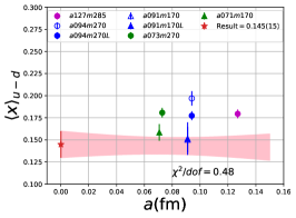
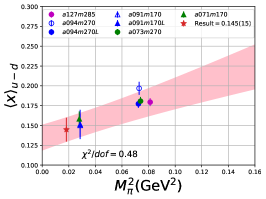
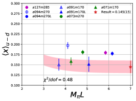
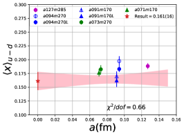
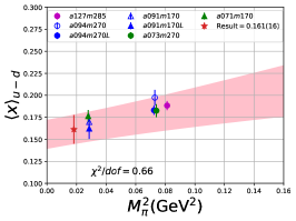
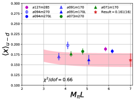
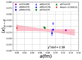
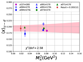
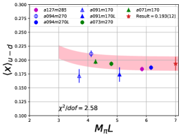
Figure 1: Data for the momentum fraction $\langle x\rangle_{u-d}$ from the seven ensembles renormalized in the $\overline{\rm MS}$ scheme at $\mu=2$ GeV. The top row shows data obtained using the $\{4^{N\pi},3^{*}\}$ fits strategy, middle from $\{4,3^{*}\}$ and bottom from $\{4,2^{\rm free}\}$. The pink band shows the result of the CCFV fit plotted versus $a$ (left panel), versus $M_{\pi}^{2}$ (middle panel) and versus $M_{\pi}L$ (right panel) with the other two variables set to their physical values in each case.

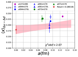
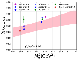
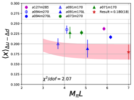
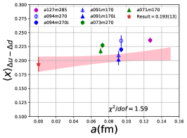
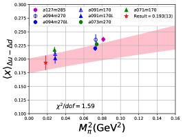
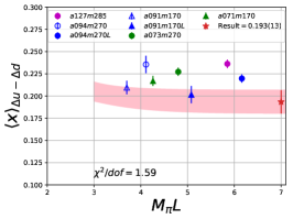
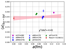
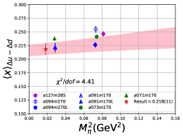
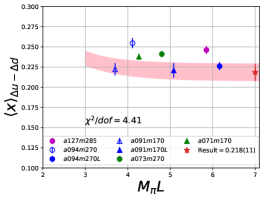
Figure 2: Data for the helicity moment $\langle x\rangle_{\Delta u-\Delta d}$ from the seven ensembles renormalized using method A (Averaging) in the $\overline{\rm MS}$ scheme at $\mu=2$ GeV. The top row shows data obtained using the $\{4^{N\pi},3^{*}\}$ fits strategy, middle from $\{4,3^{*}\}$ and bottom from $\{4,2^{\rm free}\}$. The pink band shows the result of the CCFV fit plotted versus $a$ (left panel), versus $M_{\pi}^{2}$ (middle panel) and versus $M_{\pi}L$ (right panel) with the other two variables set to their physical values in each case.

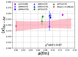
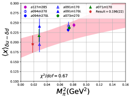
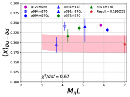
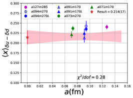
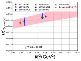
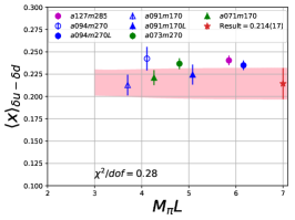
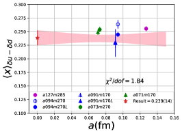
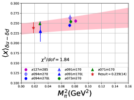
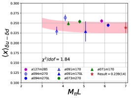
Figure 3: Data for the transversity moment $\langle x\rangle_{\delta u-\delta d}$ from the seven ensembles renormalized in the $\overline{\rm MS}$ scheme at $\mu=2$ GeV. The top row shows data obtained using the $\{4^{N\pi},3^{*}\}$ fits strategy, middle from $\{4,3^{*}\}$ and bottom from $\{4,2^{\rm free}\}$. The pink band shows the result of the CCFV fit plotted versus $a$ (left panel), versus $M_{\pi}^{2}$ (middle panel) and versus $M_{\pi}L$ (right panel) with the other two variables set to their physical values in each case.

	Renorm	$\langle x\rangle_{u-d}$		$\langle x\rangle_{\Delta u-\Delta d}$		$\langle x\rangle_{\delta u-\delta d}$
strategy	Method	CC	CCFV	CC	CCFV	CC	CCFV
$\{4^{N\pi},3^{*}\}$	A	$0.160(13)$	$0.145(15)$	$0.196(16)$	$0.180(18)$	$0.201(19)$	$0.196(22)$
$\{4^{N\pi},3^{*}\}$	B	$0.160(12)$	$0.145(15)$	$0.196(15)$	$0.178(18)$	$0.205(19)$	$0.198(22)$
$\{4^{N\pi},3^{*}\}$	Final	$0.160(13)$	$0.145(15)$	$0.196(16)$	$0.179(18)$	$0.203(19)$	$0.197(22)$
$\{4,3^{*}\}$	A	$0.170(15)$	$0.161(16)$	$0.203(11)$	$0.193(13)$	$0.215(14)$	$0.214(17)$
$\{4,3^{*}\}$	B	$0.168(14)$	$0.159(16)$	$0.201(11)$	$0.190(13)$	$0.218(14)$	$0.215(17)$
$\{4,3^{*}\}$	Final	$0.169(15)$	$0.160(16)$	$0.202(11)$	$0.192(13)$	$0.217(14)$	$0.215(17)$
$\{4,2^{\rm free}\}$	A	$0.209(11)$	$0.193(12)$	$0.2324(89)$	$0.218(11)$	$0.249(12)$	$0.239(14)$
$\{4,2^{\rm free}\}$	B	$0.206(11)$	$0.190(12)$	$0.2283(92)$	$0.213(11)$	$0.248(12)$	$0.237(14)$
$\{4,2^{\rm free}\}$	Final	$0.208(11)$	$0.192(12)$	$0.2304(92)$	$0.216(11)$	$0.249(12)$	$0.238(14)$

Table 10: The final results of the chiral-continuum-finite-volume fits for the three moments and the three strategies used to remove excited state contamination. Results are given for the two methods of renormalization (A and B) discussed in appendix B. The final value for each strategy is taken to be the average of the two estimates along with the larger of the two errors.

Collaboration	Ref.	$\langle x\rangle_{u-d}$	$\langle x\rangle_{\Delta u-\Delta d}$	$\langle x\rangle_{\delta u-\delta d}$	Remarks
NME 20		$0.160(16)(20)$	$0.192(13)(20)$	$0.215(17)(20)$	$N_{f}=2+1$
(this work)					clover-on-clover
PNDME 20	Mondal et al. (2020)	$0.173(14)(07)$	$0.213(15)(22)$	$0.208(19)(24)$	$N_{f}=2+1+1$
					clover-on-HISQ
ETMC 20	Alexandrou et al. (2020a)	$0.171(18)$			$N_{f}=2+1+1$ Twisted Mass
					N-DIS, N-FV
ETMC 19	Alexandrou et al. (2020b)	$0.178(16)$	$0.193(18)$	$0.204(23)$	$N_{f}=2+1+1$ Twisted Mass
					N-DIS, N-FV
Mainz 19	Harris et al. (2019)	$0.180(25)_{\rm stat}$	$0.221(25)_{\rm stat}$	$0.212(32)_{\rm stat}$	$N_{f}=2+1$ Clover
		$(+14,-6)_{\rm sys}$	$(+10,-0)_{\rm sys}$	$(+16,-10)_{\rm sys}$
$\chi$QCD 18	Yang et al. (2018)	$0.151(28)(29)$			$N_{f}=2+1$
					Overlap on Domain Wall
RQCD 18	Bali et al. (2019)	$0.195(07)(15)$	$0.271(14)(16)$	$0.266(08)(04)$	$N_{f}=2$ Clover
ETMC 17	Alexandrou et al. (2017)	$0.194(9)(11)$			$N_{f}=2$ Twisted Mass
					N-DIS, N-FV
ETMC 15	Abdel-Rehim et al. (2015)	$0.208(24)$	$0.229(30)$	$0.306(29)$	$N_{f}=2$ Twisted Mass
					N-DIS, N-FV
RQCD 14	Bali et al. (2014)	$0.217(9)$			$N_{f}=2$ Clover
					N-DIS, N-CE, N-FV
LHPC 14	Green et al. (2014)	$0.140(21)$			$N_{f}=2+1$ Clover
					N-DIS ($a\sim 0.12$ fm)
RBC/	Aoki et al. (2010)	0.124–0.237	0.146–0.279		$N_{f}=2+1$ Domain Wall
UKQCD 10					N-DIS, N-CE, N-ES
LHPC 10	Bratt et al. (2010)	$0.1758(20)$	$0.1972(55)$		$N_{f}=2+1$
					Domain Wall-on-Asqtad
					N-DIS, N-CE, N-NR, N-ES
CT18	Hou et al. (2019)	$0.156(7)$
JAM17†	Ethier et al. (2017); Lin et al. (2018)		0.241(26)
NNPDF3.1	Ball et al. (2017)	$0.152(3)$
ABMP2016	Alekhin et al. (2017)	$0.167(4)$
CJ15	Accardi et al. (2016b)	$0.152(2)$
HERAPDF2.0	Abramowicz et al. (2015)	$0.188(3)$
CT14	Dulat et al. (2016)	$0.158(4)$
MMHT2014	Harland-Lang et al. (2015)	$0.151(4)$
NNPDFpol1.1	Nocera et al. (2014)		$0.195(14)$
DSSV08	de Florian et al. (2009, 2008)		$0.203(9)$

Table 11: Our Lattice QCD results are compared with other lattice calculations with $N_{f}$ flavors of dynamical fermions in rows 2–9, and with results from phenomenological global fits in the remainder of the table. In both cases, the results are arranged in reverse chronological order. All results are in the $\overline{\rm MS}$ scheme at scale $2$ GeV. For a discussion and comparison of lattice and global fit results up to 2020, see Ref. Constantinou et al. (2020) and also the comparison in Hou et al. (2019) for $\langle x\rangle_{u-d}$. The JAM17^† estimate for $\langle x\rangle_{\Delta u-\Delta d}$ is obtained from Lin et al. (2018), where, as part of the review, an analysis was carried out using the data in Ethier et al. (2017). The following abbreviations are used in the remarks column for various sources of systematic uncertainties in lattice calculations—DIS: Discretization effects, CE: Chiral extrapolation, FV: Finite volume effects, NR: Nonperturbative renormalization, ES: Excited state contaminations. A prefix “N-” means that the systematic uncertainty was neither adequately controlled nor estimated.

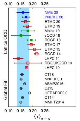
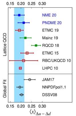
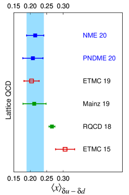
Figure 4: A comparison of results from lattice QCD calculations with dynamical fermions and global fits (below the black line) summarized in Table 11. The left panel compares results for the momentum fraction, the middle for the helicity moment, and the right for the transversity moment. Our NME 20 result is also shown as the blue band to facilitate comparison.

VII Conclusions

We have presented results for the isovector quark momentum fraction, $\langle x\rangle_{u-d}^{{\rm\overline{MS}}}$, helicity moment, $\langle x\rangle^{{\rm\overline{MS}}}_{\Delta u-\Delta d}$, and transversity moment, $\langle x\rangle^{{\rm\overline{MS}}}_{\delta u-\delta d}$ on seven ensembles with 2+1-flavor Wilson-clover fermions. Using high statistics data we confirmed the behavior of the correlation functions predicted by the spectral decomposition as shown in Figs. 5–10. These higher precision data allowed us to investigate the systematic uncertainty associated with excited-state contamination when extracting the three moments. We carried out the full analysis with three different estimates of the mass gap of the first excited state that cover a large range of possible values. We use the spread in results to assign a systematic uncertainty to account for possible residual excited-state bias.

To obtain the final result in the continuum limit, we fit the seven points using the ansatz in Eq. (77) that includes the leading order terms in $M_{\pi}$, the lattice spacing $a$ and the finite volume parameter $M_{\pi}L$. Having two pairs of points, $\{a094m270,a094m270L\}$ and $\{a091m170,a091m170L\}$, that differ only in the lattice volume, allowed us to quantify finite volume corrections in all three moments as shown in Figs. 1, 2 and 3. A comparison of the results with and without the finite-volume correction (CCFV versus CC) are shown in Table 10. Based on this analysis, we present final results from the CCFV fits that are about 5% smaller than the CC-fit values for the momentum fraction and the helicity moment. These results are consistent with the PNDME 20 Mondal et al. (2020) calculation, which used the clover-on-HISQ lattice formulation and were obtained using just CC fits.

In appendix B, we describe two methods for removing the $p^{2}$ dependent artifacts in the renormalization constants. The results for the moments from these two methods are given in Table 10. The data show that after the continuum extrapolation (CCFV or CC fits), the two estimates overlap even though the renormalization constants themselves differ by $\approx 5\%$ as shown in Table 12. The better agreement after the continuum extrapolation suggests that the main difference between the two methods are indeed discretization artifacts.

The data at three values of the lattice spacing shown in Figs. 1, 2 and 3 do not exhibit any significant dependence on the lattice spacing $a$. The main variation is with $M_{\pi}^{2}$, and its magnitude depends on the mass gap of the first excited state used in the analysis of the ESC. Since the mass gaps obtained from fits to the three-point functions ($\{4,2^{\rm free}\}$ strategy) do not prefer values corresponding to the lowest possible excitations ($N\pi$ states used in the $\{4^{N\pi},3^{*}\}$ strategy) but are closer to two-state fits to the two-point function (see Table 3), we quote final results from the $\{4,3^{*}\}$ strategy. We add a systematic error of $0.02$, based on the observed spread (see Table 10), to account for possible unresolved excited-state effects.

Our final results, taken from Table 10, are given in Eq. (78). These are compared with other lattice calculations and phenomenological global fit estimates in Table 11 and Fig. 4. They are in good agreement with other recent lattice results from the PNDME Mondal et al. (2020), ETMC Alexandrou et al. (2020a, b), Mainz Harris et al. (2019) and $\chi$QCD Yang et al. (2018) collaborations. Our estimate for the momentum fraction is in good agreement with most global fit estimates but has much larger error. The three estimates for the helicity moment from global fits have a large spread, and our estimate is consistent with the smaller error estimates. Lattice estimates for the transversity moment are a prediction.

Having established the efficacy of the lattice QCD approach to reliably calculate these isovector moments, we expect to make steady progress in reducing the errors by simulating at additional values of $\{a,M_{\pi}\}$ and by increasing the statistics.

Appendix A Plots of the Ratio $C_{\mathcal{O}}^{3\text{pt}}(\tau;t)/C^{2\text{pt}}(\tau)$

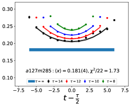
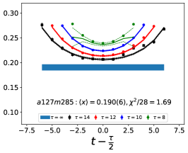
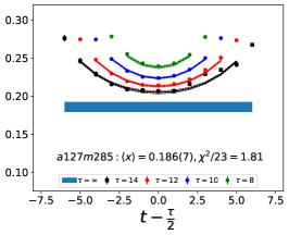
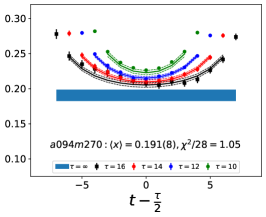
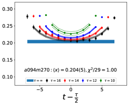
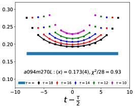
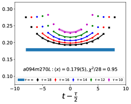
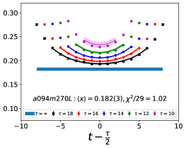
Figure 5: Data and fits to remove excited-state contamination in the extraction of the momentum fraction $\langle x\rangle_{u-d}$ for $a127m285$ (top row), $a094m270$ (second row), and $a094m270L$ (bottom row) ensembles. The data for the ratio $C_{\mathcal{O}}^{3\text{pt}}(\tau;t)/C^{2\text{pt}}(\tau)$ is scaled using Eq. (66) to give $\langle x\rangle_{u-d}$, and the fit parameters are listed in Tables 5. In each row, the three panels shows data for the three strategies: $\{4^{N\pi},3^{*}\}$ (left), $\{4,3^{*}\}$ (middle) and $\{4,2^{\rm free}\}$ (right). For each $\tau$, the line in the same color as the data points is the result of the fit used (see Sec. V) to obtain the ground state matrix element. The result for the unrenormalized ground-state value of the moment is shown by the blue band and summarized in Table 4 along with the values of $\tau$ and $t_{\rm skip}$ used in the fit. The y-interval is selected to be the same for all the panels to facilitate comparison.

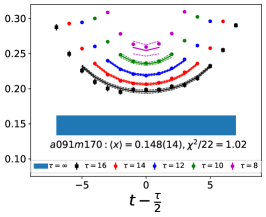
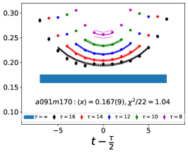
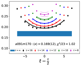
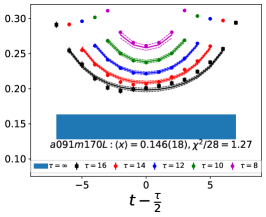
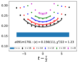
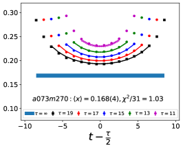
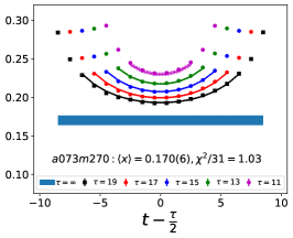
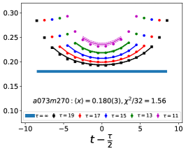
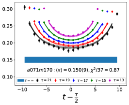
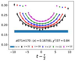
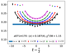
Figure 6: Continuation of the data and fits to remove excited-state contamination in the extraction of the momentum fraction $\langle x\rangle_{u-d}$ for $a091m170$ (top row), $a091m170L$ (middle row), $a073m270$ (third row), and $a071m170$ (bottom row). The data for the ratio $C_{\mathcal{O}}^{3\text{pt}}(\tau;t)/C^{2\text{pt}}(\tau)$ is scaled using Eq. (66) to give $\langle x\rangle_{u-d}$, and the fit parameters are listed in Table 5. The rest is the same as in Fig. 5.

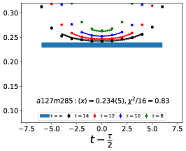
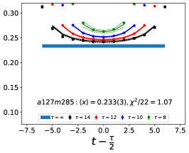
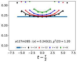
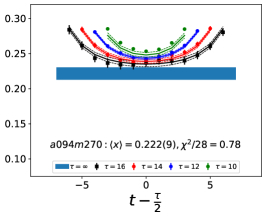
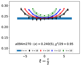
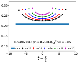
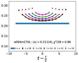
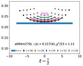
Figure 7: Data and fits to remove excited-state contamination in the extraction of the helicity moment $\langle x\rangle_{\Delta u-\Delta d}$ for for $a127m285$ (top row), $a094m270$ (second row), and $a094m270L$ (bottom row) ensembles. The data for the ratio $C_{\mathcal{O}}^{3\text{pt}}(\tau;t)/C^{2\text{pt}}(\tau)$ is scaled using Eq. (67) to give $\langle x\rangle_{\Delta u-\Delta d}$, and the fit parameters are listed in Table 6. The rest is the same as in Fig. 5.

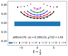
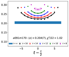
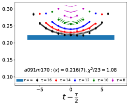
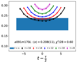
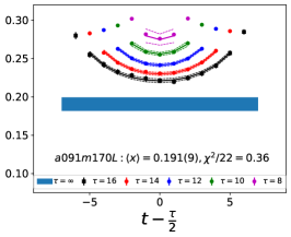
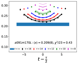
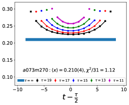
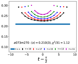
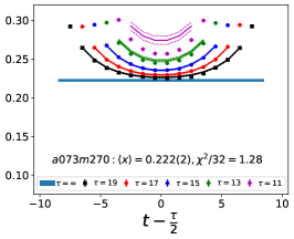
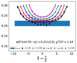
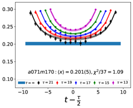
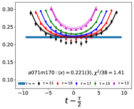
Figure 8: Continuation of the data and fits to remove excited-state contamination in the extraction of the helicity moment $\langle x\rangle_{\Delta u-\Delta d}$ for $a091m170$ (top row), $a091m170L$ (middle row), $a073m270$ (third row), and $a071m170$ (bottom row). The data for the ratio $C_{\mathcal{O}}^{3\text{pt}}(\tau;t)/C^{2\text{pt}}(\tau)$ is scaled using Eq. (67) to give $\langle x\rangle_{\Delta u-\Delta d}$, and the fit parameters are listed in Table 6. The rest is the same as in Fig. 5.

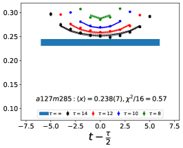
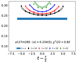
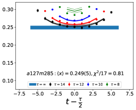
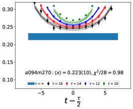
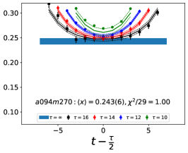
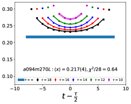
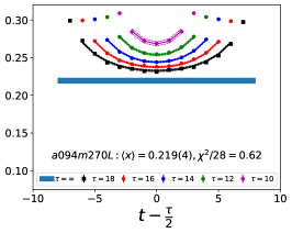
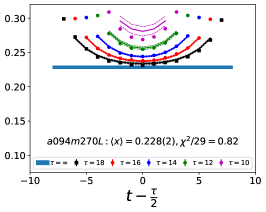
Figure 9: Data and fits to remove excited-state contamination in the extraction of the transversity moment $\langle x\rangle_{\delta u-\delta d}$ for $a127m285$ (top row), $a094m270$ (second row), and $a094m270L$ (bottom row) ensembles. The data for the ratio $C_{\mathcal{O}}^{3\text{pt}}(\tau;t)/C^{2\text{pt}}(\tau)$ is scaled using Eq. (68) to give $\langle x\rangle_{\delta u-\delta d}$, and the fit parameters are listed in Table 7. The rest is the same as in Fig. 5.

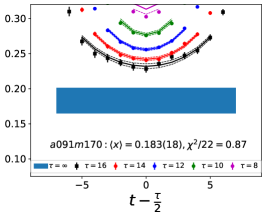
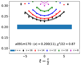
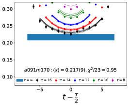
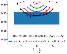
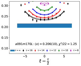
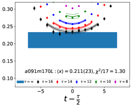
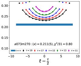
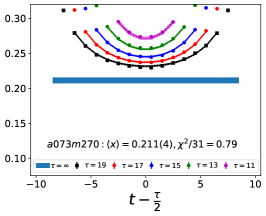
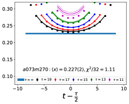
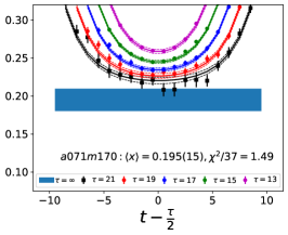
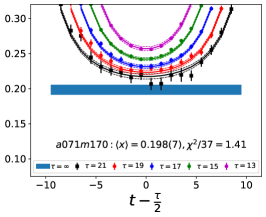
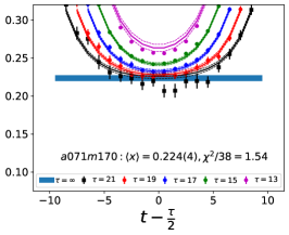
Figure 10: Continuation of the data and fits to remove excited-state contamination in the extraction of the transversity moment $\langle x\rangle_{\delta u-\delta d}$ for $a091m170$ (top row), $a091m170L$ (middle row), $a073m270$ (third row), and $a071m170$ (bottom row). The data for the ratio $C_{\mathcal{O}}^{3\text{pt}}(\tau;t)/C^{2\text{pt}}(\tau)$ is scaled using Eq. (68) to give $\langle x\rangle_{\delta u-\delta d}$, and the fit parameters are listed in Table 7. The rest is the same as in Fig. 5.

In this appendix, we show plots of the unrenormalized isovector momentum fraction, $\langle x\rangle_{u-d}$, the helicity moment, $\langle x\rangle_{\Delta u-\Delta d}$, and the transversity moment, $\langle x\rangle_{\delta u-\delta d}$, for the seven ensembles in Figs. 5–10. The data shown is the ratio $C_{\mathcal{O}}^{3\text{pt}}(\tau;t)/C^{2\text{pt}}(\tau)$ multiplied by the appropriate factor given in Eqs. (66)–(68) to get the three $\langle x\rangle$. The three panels in each row show fits with the three strategies: $\{4^{N\pi},3^{*}\}$ (left), $\{4,3^{*}\}$ (middle) and $\{4,2^{\rm free}\}$ (right). The fits to $C_{\mathcal{O}}^{3\text{pt}}(\tau;t)$ using Eq. (76) are made keeping data at the largest three values of $\tau$, except for $a071m170$ as discussed in Sec. V. The results of these fit are shown for various $\tau$ by lines with the same color as the data. In all cases, to extract the ground state matrix element (blue band), the fits to $C^{2\text{pt}}(\tau)$ and $C_{\mathcal{O}}^{3\text{pt}}(\tau;t)$ are done within a single jackknife loop.

The data show a monotonic convergence in $\tau$ towards the $\tau\to\infty$ estimate. Also, the data are symmetric about $t-\tau/2$ for all values of $\tau$, except for the largest $\tau$ on $a071m170$, $a091m170L$ and $a094m270$ ensembles, which are statistics limited. Lastly, the largest extrapolation, ie, the difference between the data at $t=\tau/2$ with the largest $\tau$ and the $\tau=\infty$ value, is for the $\{4^{N\pi},3^{\ast}\}$ strategy since it has the smallest mass gap as shown in Table 3. This is most evident on the $m_{\pi}\approx 170$ MeV ensembles. The smallest is for the $\{4,2^{\rm free}\}$ strategy in which the mass gap is the largest.

Ensemble	$N_{conf}$	fit range	Method A			Method B
		$[{\rm GeV^{2}}]$	$Z_{VD}$	$Z_{AD}$	$Z_{TD}$	$Z_{VD}$	$Z_{AD}$	$Z_{TD}$
$a127m285$	100	3.7 – 5.7	0.990(16)	1.012(17)	1.026(16)	0.941(14)	0.962(18)	0.981(17)
$a094m270$	100	5.3 – 7.3	1.036(15)	1.061(15)	1.085(15)	0.999(17)	1.030(18)	1.062(18)
$a094m270L$	100	5.3 – 7.3	1.025(14)	1.040(14)	1.071(16)	0.991(14)	1.000(15)	1.043(20)
$a091m170$	101	5.5 – 7.5	1.016(12)	1.029(14)	1.062(14)	0.977(13)	0.987(16)	1.032(16)
$a091m170L$	108	5.5 – 7.5	1.039(14)	1.058(15)	1.088(18)	0.999(16)	1.021(17)	1.056(22)
$a073m270$	100	7.1 – 9.1	1.073(17)	1.084(15)	1.120(19)	1.051(20)	1.056(17)	1.104(19)
$a071m170$	112	7.4 – 9.4	1.054(10)	1.077(11)	1.114(12)	0.996(11)	1.023(14)	1.072(15)

Table 12: Results for the renormalization factors, $Z_{VD,AD,TD}$, in the $\overline{\rm MS}$ scheme at $2$ GeV. These are calculated in the RI’-MOM scheme as a function of scale $p=\sqrt{p_{\mu}p_{\mu}}$ on the lattice, matched to the $\overline{\rm MS}$ scheme at the same scale $\mu=p$, and then run in the continuum $\overline{\rm MS}$ scheme from $\mu$ to $2$ GeV. Results are given for two methods used to remove the $p^{2}$ dependent artifacts as described in the text. In method A (columns 4–6), the $Z$’s are obtained by averaging the data shown in Fig. 11 over the range of $p^{2}$ specified in the in the third column. Results using method B (columns 7–9) are obtained using fits to the data starting with the lower value of $p^{2}$ given in column 3 with the ansatz $Z(p)=Z_{0}+ap^{2}+bp^{4}$.

Appendix B Renormalization

In this appendix, we describe two methods of calculating the renormalization factors, $Z_{VD,AD,TD}$, for the three one-derivative operators specified in Eqs. (47), (56) and (65). On the lattice, these $Z$’s are first determined nonperturbatively in the ${\rm RI}^{\prime}{\rm-MOM}$  scheme Gockeler et al. (2010); Constantinou et al. (2013) as a function of the lattice scale $p^{2}=p^{\mu}p^{\mu}$, and then converted to ${\rm\overline{MS}}$ scheme using $3$-loop perturbative factors calculated in the continuum in Ref. Gracey (2003). For data at each $p$, we perform horizontal matching by choosing the ${\rm\overline{MS}}$ scale $\mu=|p|$. These numbers are then run in the continuum ${\rm\overline{MS}}$ scheme from scale $\mu$ to $2$ GeV using three-loop anomalous dimensions Gracey (2003). The two methods differ in how the dependence of $Z^{\rm\overline{MS}}$(2GeV) on $p^{2}a^{2}$, a lattice artifact, is removed. For details of the three operators and their decomposition into irreducible representations, we refer the reader to Refs. Gockeler et al. (1996); Harris et al. (2019).

The data for the renormalization factors $Z_{VD,AD,TD}$ in the ${\rm\overline{MS}}$ scheme at $\mu=2$ GeV is shown in Fig. 11 for the seven ensembles as a function of $p^{2}$—the scale of the ${\rm RI}^{\prime}{\rm-MOM}$  scheme on the lattice. For all three operators, the data do not show a window in $p^{2}$ where the results are independent of $p^{2}$. We analyze the variation with $p^{2}$ as being mainly due to a combination of the breaking of full rotational invariance on the lattice and other $p^{2}$ dependent artifacts. Many methods have been proposed to control it, see for example Refs. Harris et al. (2019); Alexandrou et al. (2020a); Bhattacharya et al. (2016). We use the following two:

• In method A, we take an average over the data points in an interval of $2\leavevmode\nobreak\ {\rm GeV^{2}}$ about ${\hat{p}}^{2}=\Lambda/a$, where the scale $\Lambda=3$ GeV is chosen to be large enough to avoid nonperturbative effects and at which perturbation theory is expected to be reasonably well behaved. Also, this choice satisfies both ${\hat{p}}a\rightarrow 0$ and $\Lambda/{\hat{p}}\rightarrow 0$ in the continuum limit as desired. The window over which the data are averaged (given in column three of Table 12) and the error (half the height of the band) are shown by shaded bands in Figs. 11. This method was used in our previous work presented in Ref. Mondal et al. (2020).

• In method B, we make a fit to the data using the ansatz $Z(p)=Z_{0}+a\sum_{\mu}p_{\mu}p_{\mu}+b(\sum_{\mu}p_{\mu}p_{\mu})^{2}$ to remove the $p^{2}$ dependent artifacts. The starting value of $p^{2}$ is taken to be the lower limit used in method A, which is given in column three of Table 12, and by which a roughly linear in $p^{2}$ behavior is manifest. The results are shown next to the y-axis in Fig. 11 using the star symbol.

These estimates of $Z_{VD}$, $Z_{AD}$ and $Z_{TD}$ are summarized in Table 12. The discretization errors are expected to be different in the two methods, so we do not average the values of the renormalization constants but perform the full analysis, including the CCFV fits, for the two methods and compare the values of the moments after the continuum extrapolation. These final results are summarized in Table 10 and found to be consistent.

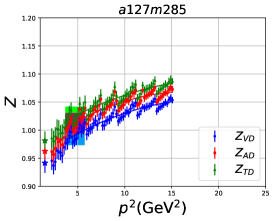
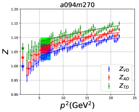
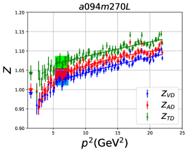
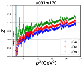
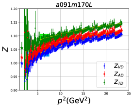
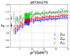
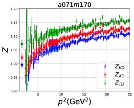
Figure 11: Nonperturbative renormalization factors for ${\langle x\rangle_{u-d}}$, ($Z_{VD}$), ${\langle x\rangle_{\Delta u-\Delta d}}$, ($Z_{AD}$), and ${\langle x\rangle_{\delta u-\delta d}}$, ($Z_{TD}$) in the ${\rm\overline{MS}}$ scheme at $\mu=2\ {\rm GeV}$ for the seven ensembles. The shaded bands mark the region in ${p^{2}}$ that is averaged and the error in the estimate. The points next to the y-axis with the star symbol give a second estimate obtained from the fit $Z(p)=Z_{0}+ap^{2}+bp^{4}$.

References

- Djawotho (2013) P. Djawotho (STAR), Nuovo Cim. C 036, 35 (2013), arXiv:1303.0543 [nucl-ex] .
- Adare et al. (2014) A. Adare et al. (PHENIX), Phys. Rev. D 90, 012007 (2014), arXiv:1402.6296 [hep-ex] .
- Dudek et al. (2012) J. Dudek et al., Eur. Phys. J. A 48, 187 (2012), arXiv:1208.1244 [hep-ex] .
- Accardi et al. (2016a) A. Accardi et al., Eur. Phys. J. A 52, 268 (2016a), arXiv:1212.1701 [nucl-ex] .
- Brock et al. (1995) R. Brock et al. (CTEQ), Rev. Mod. Phys. 67, 157 (1995).
- Ji et al. (2020) X. Ji, Y.-S. Liu, Y. Liu, J.-H. Zhang, and Y. Zhao, “Large-Momentum Effective Theory,” (2020), arXiv:2004.03543 [hep-ph] .
- Yoon et al. (2017a) B. Yoon, M. Engelhardt, R. Gupta, T. Bhattacharya, J. R. Green, B. U. Musch, J. W. Negele, A. V. Pochinsky, A. Schafer, and S. N. Syritsyn, Phys. Rev. D 96, 094508 (2017a), arXiv:1706.03406 [hep-lat] .
- Diehl (2003) M. Diehl, Generalized parton distributions, Ph.D. thesis, DESY (2003), arXiv:hep-ph/0307382 .
- Cichy and Constantinou (2019) K. Cichy and M. Constantinou, Adv. High Energy Phys. 2019, 3036904 (2019), arXiv:1811.07248 [hep-lat] .
- Karthik (2019) N. Karthik, “Lattice computations of PDF: Challenges and progress,” https://indico.cern.ch/event/764552/contributions/3420535/attachments/1864018/3064443/LatticeTalk19_NK.pdf (2019), accessed: 2020-05-20.
- Lin et al. (2018) H.-W. Lin et al., Prog. Part. Nucl. Phys. 100, 107 (2018), arXiv:1711.07916 [hep-ph] .
- Constantinou et al. (2020) M. Constantinou et al., “Parton distributions and lattice QCD calculations: toward 3D structure,” (2020), arXiv:2006.08636 [hep-ph] .
- Aoki et al. (2020) S. Aoki et al. (Flavour Lattice Averaging Group), Eur. Phys. J. C 80, 113 (2020), arXiv:1902.08191 [hep-lat] .
- Gupta et al. (2018) R. Gupta, Y.-C. Jang, B. Yoon, H.-W. Lin, V. Cirigliano, and T. Bhattacharya, Phys. Rev. D98, 034503 (2018), arXiv:1806.09006 [hep-lat] .
- Edwards et al. (2016) R. Edwards, R. Gupta, B. Joó, K. Orginos, D. Richards, F. Winter, and B. Yoon, “U.S. 2+1 flavor clover lattice generation program,” (2016), unpublished.
- Mondal et al. (2020) S. Mondal, R. Gupta, S. Park, B. Yoon, T. Bhattacharya, and H.-W. Lin, Phys. Rev. D 102, 054512 (2020), arXiv:2005.13779 [hep-lat] .
- Morningstar and Peardon (2004) C. Morningstar and M. J. Peardon, Phys. Rev. D 69, 054501 (2004), arXiv:hep-lat/0311018 .
- Sheikholeslami and Wohlert (1985) B. Sheikholeslami and R. Wohlert, Nucl. Phys. B259, 572 (1985).
- Luscher et al. (1997) M. Luscher, S. Sint, R. Sommer, P. Weisz, and U. Wolff, Nucl. Phys. B 491, 323 (1997), arXiv:hep-lat/9609035 .
- Duane et al. (1987) S. Duane, A. Kennedy, B. Pendleton, and D. Roweth, Phys. Lett. B 195, 216 (1987).
- Yoon et al. (2017b) B. Yoon et al., Phys. Rev. D 95, 074508 (2017b), arXiv:1611.07452 [hep-lat] .
- Bali et al. (2010) G. S. Bali, S. Collins, and A. Schafer, Comput.Phys.Commun. 181, 1570 (2010), arXiv:0910.3970 [hep-lat] .
- Blum et al. (2013) T. Blum, T. Izubuchi, and E. Shintani, Phys.Rev. D88, 094503 (2013), arXiv:1208.4349 [hep-lat] .
- Güsken et al. (1988) S. Güsken, K. Schilling, R. Sommer, K. H. Mütter, and A. Patel, Phys. Lett. B212, 216 (1988).
- Yoon et al. (2016) B. Yoon et al., Phys. Rev. D93, 114506 (2016), arXiv:1602.07737 [hep-lat] .
- Babich et al. (2010) R. Babich, J. Brannick, R. Brower, M. Clark, T. Manteuffel, et al., Phys.Rev.Lett. 105, 201602 (2010), arXiv:1005.3043 [hep-lat] .
- Clark et al. (2010) M. Clark, R. Babich, K. Barros, R. Brower, and C. Rebbi, Comput.Phys.Commun. 181, 1517 (2010), arXiv:0911.3191 [hep-lat] .
- Clark et al. (2016) M. A. Clark, B. Joó, A. Strelchenko, M. Cheng, A. Gambhir, and R. C. Brower, in Proceedings of the International Conference for High Performance Computing, Networking, Storage and Analysis, SC ’16 (IEEE Press, 2016) p. 68.
- Gusken et al. (1989) S. Gusken, U. Low, K. H. Mutter, R. Sommer, A. Patel, and K. Schilling, Phys. Lett. B227, 266 (1989).
- Edwards and Joo (2005) R. G. Edwards and B. Joo (SciDAC, LHPC, UKQCD), Nucl. Phys. B Proc. Suppl. 140, 832 (2005), arXiv:hep-lat/0409003 .
- Gockeler et al. (1996) M. Gockeler, R. Horsley, E.-M. Ilgenfritz, H. Perlt, P. E. L. Rakow, G. Schierholz, and A. Schiller, Phys. Rev. D53, 2317 (1996), arXiv:hep-lat/9508004 [hep-lat] .
- Harris et al. (2019) T. Harris, G. von Hippel, P. Junnarkar, H. B. Meyer, K. Ottnad, J. Wilhelm, H. Wittig, and L. Wrang, Phys. Rev. D100, 034513 (2019), arXiv:1905.01291 [hep-lat] .
- Bhattacharya et al. (2014) T. Bhattacharya, S. D. Cohen, R. Gupta, A. Joseph, H.-W. Lin, and B. Yoon, Phys. Rev. D89, 094502 (2014), arXiv:1306.5435 [hep-lat] .
- Bali et al. (2014) G. S. Bali, S. Collins, B. Gläßle, M. Göckeler, J. Najjar, R. H. Rödl, A. Schäfer, R. W. Schiel, A. Sternbeck, and W. Söldner, Phys. Rev. D90, 074510 (2014), arXiv:1408.6850 [hep-lat] .
- Bali et al. (2012) G. S. Bali, S. Collins, M. Deka, B. Glassle, M. Gockeler, J. Najjar, A. Nobile, D. Pleiter, A. Schafer, and A. Sternbeck, Phys. Rev. D86, 054504 (2012), arXiv:1207.1110 [hep-lat] .
- Jang et al. (2020) Y.-C. Jang, R. Gupta, B. Yoon, and T. Bhattacharya, Phys. Rev. Lett. 124, 072002 (2020), arXiv:1905.06470 [hep-lat] .
- Akaike (1974) H. Akaike, IEEE Transactions on Automatic Control 19, 716 (1974).
- Alexandrou et al. (2020a) C. Alexandrou, S. Bacchio, M. Constantinou, J. Finkenrath, K. Hadjiyiannakou, K. Jansen, G. Koutsou, H. Panagopoulos, and G. Spanoudes, Phys. Rev. D 101, 094513 (2020a), arXiv:2003.08486 [hep-lat] .
- Alexandrou et al. (2020b) C. Alexandrou et al., Phys. Rev. D 101, 034519 (2020b), arXiv:1908.10706 [hep-lat] .
- Yang et al. (2018) Y.-B. Yang, J. Liang, Y.-J. Bi, Y. Chen, T. Draper, K.-F. Liu, and Z. Liu, Phys. Rev. Lett. 121, 212001 (2018), arXiv:1808.08677 [hep-lat] .
- Bali et al. (2019) G. S. Bali, S. Collins, M. Göckeler, R. Rödl, A. Schäfer, and A. Sternbeck, Phys. Rev. D 100, 014507 (2019), arXiv:1812.08256 [hep-lat] .
- Alexandrou et al. (2017) C. Alexandrou, M. Constantinou, K. Hadjiyiannakou, K. Jansen, C. Kallidonis, G. Koutsou, A. Vaquero Avilés-Casco, and C. Wiese, Phys. Rev. Lett. 119, 142002 (2017), arXiv:1706.02973 [hep-lat] .
- Abdel-Rehim et al. (2015) A. Abdel-Rehim et al., Phys. Rev. D92, 114513 (2015), [Erratum: Phys. Rev.D93,no.3,039904(2016)], arXiv:1507.04936 [hep-lat] .
- Green et al. (2014) J. R. Green, M. Engelhardt, S. Krieg, J. W. Negele, A. V. Pochinsky, and S. N. Syritsyn, Phys. Lett. B734, 290 (2014), arXiv:1209.1687 [hep-lat] .
- Aoki et al. (2010) Y. Aoki, T. Blum, H.-W. Lin, S. Ohta, S. Sasaki, et al., Phys.Rev. D82, 014501 (2010), arXiv:1003.3387 [hep-lat] .
- Bratt et al. (2010) J. Bratt et al. (LHPC Collaboration), Phys.Rev. D82, 094502 (2010), arXiv:1001.3620 [hep-lat] .
- Hou et al. (2019) T.-J. Hou et al., “New CTEQ global analysis of quantum chromodynamics with high-precision data from the LHC,” (2019), arXiv:1912.10053 [hep-ph] .
- Ethier et al. (2017) J. Ethier, N. Sato, and W. Melnitchouk, Phys. Rev. Lett. 119, 132001 (2017), arXiv:1705.05889 [hep-ph] .
- Ball et al. (2017) R. D. Ball et al. (NNPDF), Eur. Phys. J. C77, 663 (2017), arXiv:1706.00428 [hep-ph] .
- Alekhin et al. (2017) S. Alekhin, J. Blümlein, S. Moch, and R. Placakyte, Phys. Rev. D96, 014011 (2017), arXiv:1701.05838 [hep-ph] .
- Accardi et al. (2016b) A. Accardi, L. T. Brady, W. Melnitchouk, J. F. Owens, and N. Sato, Phys. Rev. D93, 114017 (2016b), arXiv:1602.03154 [hep-ph] .
- Abramowicz et al. (2015) H. Abramowicz et al. (H1, ZEUS), Eur. Phys. J. C75, 580 (2015), arXiv:1506.06042 [hep-ex] .
- Dulat et al. (2016) S. Dulat, T.-J. Hou, J. Gao, M. Guzzi, J. Huston, P. Nadolsky, J. Pumplin, C. Schmidt, D. Stump, and C. P. Yuan, Phys. Rev. D93, 033006 (2016), arXiv:1506.07443 [hep-ph] .
- Harland-Lang et al. (2015) L. A. Harland-Lang, A. D. Martin, P. Motylinski, and R. S. Thorne, Eur. Phys. J. C75, 204 (2015), arXiv:1412.3989 [hep-ph] .
- Nocera et al. (2014) E. R. Nocera, R. D. Ball, S. Forte, G. Ridolfi, and J. Rojo (NNPDF), Nucl. Phys. B887, 276 (2014), arXiv:1406.5539 [hep-ph] .
- de Florian et al. (2009) D. de Florian, R. Sassot, M. Stratmann, and W. Vogelsang, Phys. Rev. D80, 034030 (2009), arXiv:0904.3821 [hep-ph] .
- de Florian et al. (2008) D. de Florian, R. Sassot, M. Stratmann, and W. Vogelsang, Phys. Rev. Lett. 101, 072001 (2008), arXiv:0804.0422 [hep-ph] .
- Gockeler et al. (2010) M. Gockeler et al., Phys. Rev. D82, 114511 (2010), [Erratum: Phys. Rev.D86,099903(2012)], arXiv:1003.5756 [hep-lat] .
- Constantinou et al. (2013) M. Constantinou, M. Costa, M. Göckeler, R. Horsley, H. Panagopoulos, H. Perlt, P. E. L. Rakow, G. Schierholz, and A. Schiller, Phys. Rev. D87, 096019 (2013), arXiv:1303.6776 [hep-lat] .
- Gracey (2003) J. A. Gracey, Nucl. Phys. B667, 242 (2003), arXiv:hep-ph/0306163 [hep-ph] .
- Bhattacharya et al. (2016) T. Bhattacharya, V. Cirigliano, S. Cohen, R. Gupta, H.-W. Lin, and B. Yoon, Phys. Rev. D94, 054508 (2016), arXiv:1606.07049 [hep-lat] .