Predominance of non-adiabatic effects in zero-point renormalization of the electronic band gap.

Abstract

Electronic and optical properties of materials are affected by atomic motion through the electron-phonon interaction: not only band gaps change with temperature, but even at absolute zero temperature, zero-point motion causes band-gap renormalization. We present a large-scale first-principles evaluation of the zero-point renormalization of band edges beyond the adiabatic approximation. For materials with light elements, the band gap renormalization is often larger than 0.3 eV, and up to 0.7 eV. This effect cannot be ignored if accurate band gaps are sought. For infrared-active materials, global agreement with available experimental data is obtained only when non-adiabatic effects are taken into account. They even dominate zero-point renormalization for many materials, as shown by a generalized Fröhlich model that includes multiple phonon branches, anisotropic and degenerate electronic extrema, whose range of validity is established by comparison with first-principles results.

This is a post-peer-review, pre-copy-edited version of the article published in npj Computational Materials (2020) 6:167. The final authenticated version is available online at: http://dx.doi.org/10.1038/s41524-020-00434-z
Note that the supplementary material, included in the main file, is structured differently than in the published version, with a different numbering scheme.

The electronic band gap is arguably the most important characteristic of semiconductors and insulators. It determines optical and luminescent thresholds, but is also a prerequisite for characterizing band offsets at interfaces and deep electronic levels created by defects Yu and Cardona (2010). However, accurate band gap computation is a challenging task. Indeed, the vast majority of first-principles calculations relies on Kohn-Sham Density-Functional Theory (KS-DFT), valid for ground state properties Martin (2004), that delivers a theoretically unjustified value of the band gap in the standard approach, even with exact KS potential Perdew and Levy (1983); Sham and Schlüter (1983); Martin, Reining, and Ceperley (2016).

The breakthrough came from many-body perturbation theory, with the so-called GW approximation, first non-self-consistent (G₀W₀) by Hybertsen and Louie in 1986 Hybertsen and Louie (1986), then twenty years later self-consistent (GW) van Schilfgaarde, Kotani, and Faleev (2006) and further improved by accurate vertex corrections from electron-hole excitations (GWeh) Shishkin, Marsman, and Kresse (2007). The latter methodology, at the forefront for band-gap computations, delivers a 2%-10% accuracy, usually overestimating the experimental band gap. GWeh calculations are computationally very demanding, typically about two orders of magnitude more than G₀W₀, itself two orders of magnitude more time-consuming than KS-DFT calculations, roughly speaking.

Despite being state-of-the-art, such studies ignored completely the electron-phonon interaction. The electron-phonon interaction drives most of the temperature dependence of the electronic structure of semiconductors and insulators, but also yields a zero-point motion gap modification at $T=0$ K, often termed zero-point renormalization of the gap (ZPR_g) for historical reasons.

The ZPR_g had been examined 40 years ago, by Allen, Heine and Cardona (AHC) Allen and Heine (1976); Allen and Cardona (1981) who clarified the early theories by Fan Fan (1951) and Antoncik Antoncik (1955). Their approach is, like the GW approximation, rooted in many-body perturbation theory, where, at the lowest order, two diagrams contribute, see Fig. 1, the so-called “Fan" diagram, with two 1^st-order electron-phonon vertices and the “ Debye-Waller" diagram, with one 2^nd-order electron-phonon vertex. In the context of semi-empirical calculations, the AHC method was applied to Si and Ge, introducing the adiabatic approximation, in which the phonon frequencies are neglected with respect to electronic eigenenergy differences and replaced by a small but non-vanishing imaginary broadening Allen and Cardona (1981). It was later extended without caution to GaAs and a few other III-V semiconductors Kim, Lautenschlager, and Cardona (1986); Zollner, Gopalan, and Cardona (1991).

In this work, we present first-principles AHC ZPR_g calculations beyond the adiabatic approximation, for 30 materials. Comparing with experimental band gaps, we show that adding ZPR_g improves the GWeh first-principles band gap, and moreover, that the ZPR_g has the same order of magnitude as the G₀W₀ to GWeh correction for half of the materials (typically materials with light atoms, e.g. O, N …) on which GWeh has been tested. Hence, the GWeh level of sophistication misses its target for many materials with light atoms, if the ZPR_g is not taken into account. With it, the theoretical agreement with direct measurements of experimental ZPR_g is improved. This also demonstrate the crucial importance of phonon dynamics to reach this level of accuracy.

Indeed, first-principles calculations of the ZPR_g using the AHC theory are very challenging, and only started one decade ago, on a case-by-case basis (see Refs Marini (2008); Giustino, Louie, and Cohen (2010); Cannuccia and Marini (2011); Gonze, Boulanger, and Côté (2011); Cannuccia and Marini (2012); Kawai et al. (2014); Poncé et al. (2014a, b); Antonius et al. (2015); Poncé et al. (2015); Nery et al. (2018); not (a), and the SI II.D), usually relying on the adiabatic approximation, and without comparison with experimental data. An approach to the ZPR_g, alternative to the AHC one, relies on computations of the band gap at fixed, distorted geometries, for large supercells (see Refs.) Capaz et al. (2005); Gonze, Boulanger, and Côté (2011); Patrick and Giustino (2013); Monserrat, Drummond, and Needs (2013); Antonius et al. (2014); Monserrat et al. (2014); Monserrat and Needs (2014); Monserrat, Engel, and Needs (2015); Engel, Monserrat, and Needs (2015) and the SI not (a), Sec.II.D). As the adiabatic approximation is inherent in this approach, we denote it as ASC, for “adiabatic supercell". A recent publication by Karsai and co-workers Karsai et al. (2018) presents ASC ZPR_g based on DFT values as well as based on G₀W₀ values for 18 semiconductors, with experimental comparison for 9 of them. Both AHC and ASC methodologies have been recently reviewed Giustino (2017).

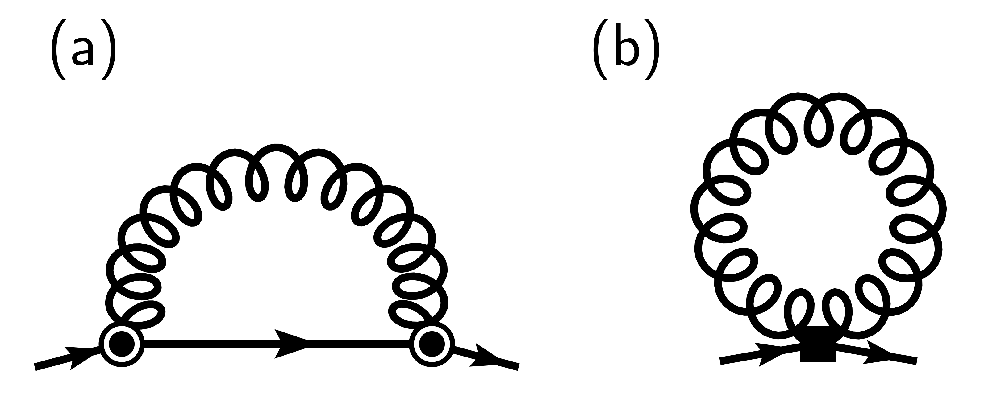
Figure 1: Lowest-order diagrams for the contribution of the electron-phonon interaction to the zero-point renormalization of the gap ZPR_g. (a) Fan diagram, with two first-order screened electron-phonon vertices; (b) Debye-Waller diagram, with one second-order screened electron-phonon interaction vertex.

Although the adiabatic approximation had already been criticized by Poncé et al. in 2015 Poncé et al. (2015) (SI Sec.III.A) as causing an unphysical divergence of the adiabatic AHC expression for infrared-active materials with vanishing imaginary broadening, thus invalidating all adiabatic AHC calculations except for non- infrared-active materials, the full consequences of the adiabatic approximation have not yet been recognized for ASC. We will show that the non-adiabatic AHC approach outperforms the ASC approach, so that the predictions arising from the mechanism by which the ASC approach bypass the adiabatic AHC divergence problem for infrared-active materials are questionable. This is made clear by a generalized Fröhlich model with a few physical parameters, that can be determined either from first principles or from experimental data.

Although the full electronic and phonon band structures do not enter in this model, and the Debye-Waller diagram is ignored, for many materials it accounts for more than half the ZPR_g of the full first-principles non-adiabatic AHC ZPR_g. As this model depends crucially on non-adiabatic effects, it demonstrates the failure of the adiabatic hypothesis be it for the AHC or the ASC approach.

By the same token, we also show the domain of validity and accuracy of model Fröhlich large-polaron calculations based on the continuum hypothesis, that have been the subject of decades of research Fröhlich (1954); Feynman (1955); Mishchenko et al. (2000, 2003); Devreese and Alexandrov (2009); Emin (2012); Hahn et al. (2018). Such model Fröhlich Hamiltonian capture well the ZPR for about half of the materials in our list, characterized by their strong infrared activity, while it becomes less and less adequate for decreasing ionicity. In the present context, the Fröhlich large-polaron model provides an intuitive picture of the physics of the ZPR_g.

Results

Zero-point renormalization: experiment versus first principles.

Fig. 2 compares first-principles ZPR_g with experimental values. As described in the METHODS section, and in SI Sec.II.C, the correction due to zero-point motion effect on the lattice parameter, ZPR${}^{\rm lat}_{\rm g}$, has been added to fixed volume results from both non-adiabatic AHC (present calculations) and ASC methodologies Karsai et al. (2018). While for a few materials experimental ZPR_g values are well established, within 5-10%, globally, experimental uncertainty is larger, and can hardly be claimed to be better than 25% for the majority of materials, see Sec.II.A in the SI. This will be our tolerance.

Let us focus first on the ASC-based results. For the 16 materials present in both Ref. Karsai et al., 2018 and the experimental set described in the SI Table S1, the ASC vs experimental discrepancy is more than 25% for more than half of the materials  not (b). There is a global trend to underestimation by ASC, although CdTe is overestimated.

By contrast, the non-adiabatic AHC ZPR_g (blue full circles) and experimental ZPR_g agree with each other within 25% for 16 out of the 18 materials. The outliers are CdTe with a 43% overestimation by theory and GaP with a 33% underestimation. For none of these the discrepancy is a factor of two or larger. On the contrary, from the ASC approaches, several materials show underestimation of the ZPR_g by more than a factor of 2. The materials showing such large underestimation (CdS, ZnO, SiC) are all quite ionic, while more covalent materials (C, Si, Ge, AlSb, AlAs) are better described.

Therefore, Fig. 2 clearly shows that the non-adiabatic AHC approach performs significantly better than the ASC approach. AHC ZPR_g and ASC ZPR_g also differ by more than a factor of two for TiO₂ and MgO (see SI Sec.II.D), although no experimental ZPR_g is available for these materials to our knowledge.

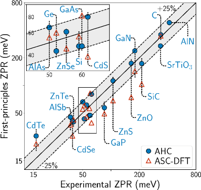
Figure 2: Absolute values of first-principles band gap renormalization ZPR_g compared with experimental ones. Blue full circles: present calculations, using non-adiabatic AHC, based on KS-DFT ingredients; red empty triangles: adiabatic supercell KS-DFT Dashed lines: limits at which the smallest of both ZPR is 25% smaller than the largest one (note that the scales are logarithmic). For consistency, the computed lattice ZPR${}^{\rm lat}_{\rm g}$ were added to both ASC and AHC. The majority of non-adiabatic AHC-based results fall See numerical values in Table S2 of the SI.

We now examine band gaps. Fig. 3 presents the ratio between first-principles band gaps and corresponding experimental values, for 12 materials. The best first-principles values at fixed equilibrium atomic position, from GWeh Shishkin, Marsman, and Kresse (2007), are represented, as well as their non-adiabatic AHC ZPR corrected values.

For GWeh without ZPR_g, a 4% agreement is obtained only for two materials (CdS and GaN). There is indeed a clear, albeit small, tendency of GWeh to overestimate the band gap value, except for the 3 materials containing shallow core d-electrons (ZnO, ZnS and CdS) that are underestimated. By contrast, if the non-adiabatic AHC ZPR_g is added to the GWeh data (blue dots), a 4% agreement is obtained for 9 out of the 12 materials (8 if ZPR${}^{\rm lat}_{\rm g}$ is not included).

For ZnO and ZnS, with a final 10-12% underestimation, and CdS with a 5% underestimation, we question the GWeh ability to produce accurate fixed-geometry band gaps at the level obtained for the other materials, due to the presence of rather localized 3d electrons in Zn and 4d electrons in CdS.

As a final lesson from Fig. 3, we note that for 4 out of the 12 materials (SiC, AlP, C, and BN), the ZPR_g is of similar size than the G₀W₀ to GWeh correction, and it is a significant fraction of it also for Si, GaN and MgO. As mentioned earlier, GWeh calculations are much more time-consuming than G₀W₀ calculations, possibly even more time-consuming than ZPR calculations (although we have not attempted to make a fair comparison). Thus, for materials containing light elements, first row and likely second row (e.g. AlP) in the periodic table, GWeh calculations miss their target if not accompanied by ZPR_g calculations. A review of the variance and accuracy of G₀W₀ calculations for these materials is discussed in Ref. Rangel et al., 2020.

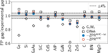
Figure 3: Ratio between first-principles band gaps and experimental ones Cardona and Thewalt (2005). First-principles results without electron-phonon interationShishkin, Marsman, and Kresse (2007) are based on G₀W₀ (diamonds) or on GWeh (squares). Blue full circles are the GWeh results to which AHC ZPR_g and lattice ZPR${}^{\rm lat}_{\rm g}$ have been added, while empty red circles are the GWeh results to with only AHC ZPR_g was added. GWeh usually overshoots, while adding the electron-phonon interaction gives better global agreement. See numerical values in Table S3 of the SI.

Table S5 of the SI gathers our full set of ZPR results, beyond those present in the ASC or experimental sets. It also includes 10 oxides, while the experimental set only includes three materials containing oxygen (ZnO, MgO and SrTiO₃), and there are none in Karsai’s ASC set. The ZPR_g of the band gap for materials containing light elements (O or lighter) is between -157 meV (ZnO) and -699 meV (BeO), while, relatively to the experimental band gap, it ranges from -4.6% (ZnO) to -10.8% (TiO₂-t). This can hardly be ignored in accurate calculations of the gap.

Generalized Fröhlich model.

We now come back to the physics from which the ZPR_g originates, and explain our earlier observation that the ASC describes reasonably well the more covalent materials, but can fail badly for ionic materials. We argue that, for many polar materials, the ZPR_g is dominated by the diverging electron-phonon interaction between zone-center LO phonons and electrons close to the band edges, and the slow (non-adiabatic) response of the latter: the effects due to comparatively fast phonons are crucial. This was already the message from Fröhlich Fröhlich (1954) and Feynman Feynman (1955), decades ago, initiating large-polaron studies. However, large-scale assessment of the adequacy of Fröhlich model for real materials is lacking. Indeed, the available flavors of Fröhlich model, based on continuum (macroscopic) electrostatic interactions, do not cover altogether degenerate and anisotropic electronic band extrema or are restricted to only one phonon branch, unlike most real materials Mahan (1965); Trebin and Rössler (1975); Devreese et al. (2010); Schlipf, Poncé, and Giustino (2018).

In this respect, we introduce now a generalized Fröhlich model, gFr, whose form is deduced from first-principles equations in the long-wavelength limit (continuum approximation). Such model covers all situations and still uses as input only long-wavelength parameters, that can be determined either from first principles (SI Sec.IV.D) or from experiment (SI Sec.IV.E). We then find the corresponding ZPR_g from perturbation theory at the lowest order, evaluate it for our set of materials, and compares its results to the ZPR_g obtained from full first-principles computations. The corresponding Hamiltonian writes (see the SI Sec.IV.B for detailed explanations):

$$\hat{H}^{\rm gFr}=\hat{H}^{\rm gFr}_{\rm el}+\hat{H}^{\rm gFr}_{\rm ph}+\hat{H}^{\rm gFr}_{\rm EPI}\,,$$ (1)

with (i) an electronic part

$$\hat{H}^{\rm gFr}_{\rm el}=\sum_{\mathbf{k}n}\frac{k^{2}}{2m^{*}_{n}(\hat{\mathbf{k}})}\hat{c}^{+}_{\mathbf{k}n}\hat{c}_{\mathbf{k}n}\,,$$ (2)

that includes direction-dependent effective masses $m^{*}_{n}(\hat{\mathbf{k}})$, governed by so-called Luttinger parameters in case of degeneracy, electronic creation and annihilation operators, $\hat{c}^{+}_{\mathbf{k}n}$ and $\hat{c}_{\mathbf{k}n}$, with $\mathbf{k}$ the electron wavevector and $n$ the band index, (ii) the multi-branch phonon part,

$$\hat{H}^{\rm gFr}_{\rm ph}=\sum_{\mathbf{q}j}\omega_{j0}(\hat{\mathbf{q}})\hat{a}^{+}_{\mathbf{q}j}\hat{a}_{\mathbf{q}j}\,,$$ (3)

with direction-dependent phonon frequencies $\omega_{j0}(\hat{\mathbf{q}})$, phonon creation and annihilation operators, $\hat{a}^{+}_{\mathbf{q}j}$ and $\hat{a}_{\mathbf{q}j}$, with $\mathbf{q}$ the phonon wavevector and $j$ the branch index, and finally (iii) the electron-phonon interaction part

$$\hat{H}^{\rm gFr}_{\rm EPI}=\sum_{\mathbf{q}j,\mathbf{k}n^{\prime}n}g^{\rm gFr}(\mathbf{q}j,\mathbf{k}n^{\prime}n)\hat{c}^{+}_{\mathbf{k}+\mathbf{q}n^{\prime}}\hat{c}_{\mathbf{k}n}(\hat{a}_{\mathbf{q}j}+\hat{a}^{+}_{-\mathbf{q}j})\,.$$ (4)

The $\mathbf{k}$ and $\mathbf{q}$ sums run over the Brillouin zone. The sum over $n$ and $n^{\prime}$ runs only over the bands that connect to the degenerate extremum, renumbered from 1 to $n_{\rm deg}$. The generalized Fröhlich electron-phonon interaction Vogl (1976); Verdi and Giustino (2015) is

$$g^{\rm gFr}(\mathbf{q}j,\mathbf{k}n^{\prime}n)=\frac{i}{q} \frac{4\pi}{\Omega_{0}}\Big{(}\frac{1}{2\omega_{j0}(\hat{\mathbf{q}})V_{\rm BvK}}\Big{)}^{1/2}\frac{\hat{\mathbf{q}}.\mathbf{p}_{j}(\hat{\mathbf{q}})}{\epsilon^{\infty}(\hat{\mathbf{q}})}$$

$$\times \sum_{m}s_{n^{\prime}m}(\hat{\mathbf{k}}^{\prime})(s_{nm}(\hat{\mathbf{k}}))^{*}.$$ (5)

This expression depends on the directions $\hat{\mathbf{k}}$, $\hat{\mathbf{q}}$, and $\hat{\mathbf{k}}^{\prime}$ ($\mathbf{k}^{\prime}=\mathbf{k}+\mathbf{q}$), but not explicitly on their norm (hence only long-wavelength parameters are used), except for the $\frac{1}{q}$ factor. The electron-phonon part also depends only on few quantities: the Born effective charges (entering the mode-polarity vectors $\mathbf{p}_{j}$), the macroscopic dielectric tensor $\epsilon^{\infty}$, and the phonon frequencies $\omega_{j0}$, the primitive cell volume $\Omega_{0}$, the Born-von Karman normalisation volume $V_{\rm BvK}$ corresponding to the $\mathbf{k}$ and $\mathbf{q}$ samplings. The $s$ tensors are symmetry-dependent unitary matrices, similar to spherical harmonics. Eqs. (1-29) define our generalized Fröhlich Hamiltonian. Although we will focus on its $T=0$ properties within perturbation theory, such Hamiltonian could be studied for many different purposes (non-zero T, mobility, optical responses …), like the original Fröhlich model, for representative materials using first-principles or experimental parameters.

The corresponding ZPR${}^{\rm gFr}_{\rm c}$ can be obtained with a perturbation treatment (SI Sec.IV.C), giving

$${\rm ZPR}_{\rm c}^{\rm gFr} = -\sum_{jn}\frac{1}{\sqrt{2}\Omega_{0}{\color[rgb]{0,0,0}n_{\rm deg}}}\int_{4\pi}d\hat{\mathbf{q}}\big{(}m_{n}^{*}(\hat{\mathbf{q}})\big{)}^{1/2}$$ (6)

$$\times \big{(}\omega_{j0}(\hat{\mathbf{q}})\big{)}^{-3/2}\Big{(}\frac{\hat{\mathbf{q}}.\mathbf{p}_{j}(\hat{\mathbf{q}})}{\epsilon^{\infty}(\hat{\mathbf{q}})}\Big{)}^{2}.$$

A similar expression exists for the valence ZPR${}^{\rm gFr}_{\rm v}$. The few material parameters needed in Eq. (39) can be obtained from experimental measurements, but are most easily computed from first principles, using density-functional perturbation theory with calculations only at $\mathbf{q}=\Gamma$ (e.g. no phonon band structure calculation). Eq. (39) can be evaluated for all band extrema in our set of materials, irrespective of whether the extrema are located at $\Gamma$ or other points in the Brillouin Zone (e.g. X for the valence band of many oxides, with anisotropic effective mass), whether they are degenerate (e.g. the three-fold degeneracy of the top of the valence band of many III-V or II-VI compounds), and irrespective of the number of phonon branches (e.g. 3 different LO frequencies for TiO₂, moreover varying with the direction along which $\mathbf{q}$ $\rightarrow 0$).

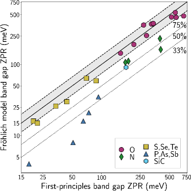
Figure 4: Zero-point renormalization of the band gap: comparison between first-principles AHC values and the values obtained from the generalized Fröhlich model fed with first-principles values, see Eq. (39), for 27 materials (non-ionic group IV materials are omitted). The markers identify materials of similar ionicity: oxides (purple circles), other II-VI materials containing S, Se or Te (yellow squares), nitrides (green diamonds), other III-V materials, containing P, As, or Sb (dark blue triangles), and group IV material SiC (light blue hexagon). Dashed lines: limits at which the smallest of both ZPR is 25% smaller than the largest one. Dotted lines: limits at which the Fröhlich model ZPR misses respectively 50% and 66% of the AHC values (note that the scales are logarithmic). See numerical values in Table S5 of the SI.

Fig. 4 compares the band gap ZPR from the first-principles non-adiabatic AHC methodology and from the generalized Fröhlich model.

The 30 materials can be grouped into five sets, based on their ionicity: 11 materials containing oxygen, rather ionic, for which the Born effective charges and the ZPR are quite large, 6 materials containing chalcogenides, also rather ionic, 4 materials containing nitrogen and 5 III-V materials, less ionic, and 4 materials from group-IV elements, non-ionic, except SiC.

For oxygen-based materials, the ZPR ranges from 150 meV to 700 meV, and the gFr model captures this very well, with less than 25% error, with only one exception, BeO. The chalcogenide materials are also reasonably well described by the gFr model, capturing at least two-third of the ZPR. Globally their ZPR is smaller (note the logarithmic scale).

For the nitride materials and for SiC, the gFr captures about 50% of the quite large ZPR (between 176 meV and 406 meV). The adequacy of the gFr model decreases still with the III-V materials and the three non-ionic IV materials. In the latter case, the vanishing Born effective charges result in a null ZPR within the gFr model. (These three materials are omitted from Fig. 4).

For the oxydes and chalcogenides, the ZPR is thus dominated by the zone-center parameters (including the phonon frequencies), and the physics corresponds to the one of the large-polaron picture Feynman (1955), namely, the slow electron motion is correlated to a phonon cloud that dynamically adjusts to it. This physics is completely absent from the ASC approach. Even for nitrides, the gFr describes a significant fraction of the ZPR.

A perfect agreement between the non-adiabatic AHC first-principles ZPR and the generalized Fröhlich model ZPR is not expected. Indeed, differences can arise from different effects: lack of dominance of the Fröhlich electron-phonon interaction in some regions of the Brillouin Zone, departure from parabolicity of the electronic structure (obviously, the electronic structure must be periodic so that the parabolic behavior does not extend to infinity), interband contributions, phonon band dispersion, incomplete cancellation between the Debye-Waller and the acoustic phonon mode contribution.

It is actually surprising to see that for so many materials, the generalized Fröhlich model matches largely the first-principles AHC results. Anyhow, as a conclusion for this section, for a large number of materials, we have validated, a posteriori and from first principles, the relevance of large-polaron research based on Fröhlich model despite the numerous approximations on which it relies.

Discussion

We focus on the mechanism by which the AHC divergence of the ZPR in the adiabatic case for infrared-active materials Poncé et al. (2015) is avoided, either using the ASC methodology or using the non-adiabatic AHC methodology. As Fröhlich and Feynman have cautioned us Fröhlich (1954); Feynman (1955), and already mentioned briefly in previous sections, the dynamics of the “slow” electron is crucial in this electron-phonon problem.

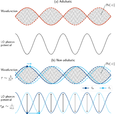
Figure 5: Schematic representation of the long-wave phonon-induced potential and corresponding electronic wavefunction, real part (oscillating with lattice periodicity) and envelope: (a) Adiabatic case, (b) non-adiabatic, time-dependent case. In the non-adiabatic case, the electron does not have the time to adjust to the change of potential, see text.

In the ASC approach, the bypass of this divergence can be understood as follows, see Fig. 5(a). Consider a long-wavelength fluctuation of the atomic positions, frozen in time. At large but finite wavelength, the potential is periodically lowered in some regions of space and increased in some other regions of space, in an oscillatory manner with periodicity $\Delta L\propto 1/q$, where $\mathbf{q}$ is the small wavevector of the fluctuation, see Fig. 5(a) "LO phonon potential" part. Without such long-wavelength potential, the electron at the minimum of the conduction band has a Bloch type wavefunction, with an envelope phase factor characterized by the wavevector $\mathbf{k}_{\rm c}$ multiplying a lattice-periodic function. Its density is lattice periodic. With such long-wavelength potential, as a function of the amplitude of the atomic displacements, the corresponding electronic eigenenergy changes first quadratically (as the average of the lowering and increase of potential for this Bloch wavefunction forbids a linear behaviour except in case of degeneracy), but for larger amplitudes, it behaves linearly, as the electron localizes in the lowered potential region and the minimum of the potential is linear in the amplitude of the atomic displacements. This is referred to as "nonquadratic coupling" in Ref. Monserrat, Engel, and Needs, 2015. A wavepacket is formed, by combining Bloch wavefunctions with similar lattice periodic functions but slightly different wavevectors ($\mathbf{k}_{\rm c}$, $\mathbf{k}_{\rm c}+\mathbf{q}$, $\mathbf{k}_{\rm c}-\mathbf{q}$, etc), coming from a small interval of energy $\Delta\epsilon^{0}\propto q^{2}\propto 1/(\Delta L)^{2}$, see Fig. 5(a) "Wavefunction" part. This nonquadratic effect is actually illustrated in Fig. 4 of Ref. Antonius et al., 2015 (see the frozen-phonon eigenvalues), as well as in Fig. 2 of Ref. Monserrat, Engel, and Needs, 2015.

By contrast, in the time-dependent case, as illustrated in Fig. 5(b), the wavepacket will require a characteristic time $\Delta\tau$, to form or to displace. This will be given by the Heisenberg uncertainty relation, $\Delta\epsilon^{0}\Delta\tau\gtrsim\hbar$, hence $\Delta\tau\gtrsim\hbar/\Delta\epsilon^{0}\propto\Delta L^{2}$. For long wavelengths, the characteristic time diverges. As soon as $\Delta\tau$ is larger than the phonon characteristic time $\tau_{\rm ph}\sim 1/\omega_{{\rm LO}}$, the “slow” electron will lag behind the phonon, and the static or adiabatic picture described above is no longer valid.

In all adiabatic approaches, either AHC or ASC, the electron is always supposed to have the time to adjust to the change of potential, in contradiction with the time-energy uncertainty principle. Furthermore, the adiabatic AHC approach only considers the quadratic region for the above-mentioned dependence of eigenvalues with respect to amplitudes of displacements. This results in a diverging term Poncé et al. (2015). At variance with the AHC case, the ASC approach samples a whole set of amplitudes, including the onset of the asymptotic linear regime, in which case the divergence does not build up. However, this ASC picture does not capture the real physical mechanism that prevent the divergence to occur, the impossibility for the electron to follow the phonon dynamics, that we have highlighted above. By contrast, such physical mechanism is present both in the non-adiabatic AHC approach and in the (generalized) Fröhlich model: the “slow" electron does not follow adiabatically (instantaneously) the atomic motion. The divergence of the adiabatic AHC is indeed avoided in the non-adiabatic picture by taking into account the non-zero phonon frequencies.

Thus the ASC avoids the adiabatic AHC divergence for the wrong reason, which explains its poor predictive capability for the more ionic materials emphasized by Fig. 2. To be clear, we do not pretend the nonquadratic effects are all absent, but the non-adiabatic effects have precedence, at least for materials with significant infrared activity, and the nonquadratic localization effects will be observed only if the electrons have the time to physically react. The shortcomings of the ASC approach are further developed in the SI Sec.V, and as a consequence of such understanding, all the results obtained for strongly infrared-active materials using the adiabatic frozen-phonon supercell methodology should be questioned.

For non-infrared-active materials, the physical picture that we have outlined, namely the inability of slow electrons to follow the dynamics of fast phonons, is still present, but does not play such a crucial role: the electron-phonon interaction by itself does not diverge in the long-wavelength limit as compared to the infrared-active electron-phonon interaction, see Eq. (29), only the denominator of the Fan self-energy diverges, which nevertheless results in an integrable ZPR Poncé et al. (2015). In such case, neglecting non-adiabatic effects, as in the ASC approach, is only one among many approximations done to obtain the ZPR.

Beyond the discovery of the predominance of non-adiabatic effects in the zero-point renormalization of the band gap for many materials, in the present large-scale first-principles study of this effect, we have established that electron-phonon interaction diminishes the band gap by 5% to 10% for materials containing light atoms like N or O (up to 0.7 eV for BeO), a decrease that cannot be ignored in accurate calculations of the gap. Our methodology, the non-adiabatic Allen-Heine-Cardona approach, has been validated by showing that, for nearly all materials for which experimental data exists, it achieves quantitative agreement (within 25%) for this property.

We have also shown that most of the discrepancies with respect to experimental data of the (arguably) best available methodology for the first-principles band-gap computation, denoted GWeh, originate from the first-principles zero-point renormalization: after including it, the average overestimation from GWeh nearly vanishes. There are some exceptions, materials in which transition metals are present, for which the addition of zero-point renormalization worsens the agreement of the band gap. For the latter materials, we believe that the GWeh approach is not accurate enough.

METHODS

First-principles electronic and phonon band structures. Calculations have been performed using ABINIT Gonze et al. (2016) with norm-conserving pseudopotentials and a plane-wave basis set. Table S1 of the SI provides calculation parameters: plane-wave kinetic cut-off energy, electronic wavevector sampling in the BZ, and largest phonon wavevector sampling in the BZ. For most of the materials, the GGA-PBE exchange-correlation functional Perdew, Burke, and Ernzerhof (1996) has been used and the pseudopotentials have been taken from the PseudoDojo project van Setten et al. (2018). For diamond, BN-zb, and AlN-wz, results reported here come from Ref. Poncé et al., 2015, where the LDA has been used, with other types of pseudopotentials.

The calculations have been performed at the theoretical optimized lattice parameter, except for Ge for which the gap closes at such parameter, for GaP, as at such parameter the conduction band presents unphysical quasi-degenerate valleys, and for TiO₂, as the GGA-PBE predicted structure is unstable Montanari and Harrison (2002). For these, we have used the experimental lattice parameter. The case of SrTiO₃ is specific and will be explained later.

Density-functional perturbation theory Baroni et al. (2001); Gonze and Lee (1997); Laflamme Janssen et al. (2016) has been used for the phonon frequencies, dielectric tensors, Born effective charges, effective masses, and electron-phonon matrix elements.

First-principles calculations of zero-point renormalization. We first detail the method used for the AHC calculations. In the many-body perturbation theory approach, an electronic self-energy $\Sigma$ appears due to the electron-phonon interaction, with Fan and Debye-Waller contributions at the lowest order of perturbation Giustino (2017):

$$\Sigma_{\mathbf{k}n}(\omega)=\Sigma^{\mathrm{Fan}}_{\mathbf{k}n}(\omega)+\Sigma^{\mathrm{DW}}_{\mathbf{k}n}.$$ (7)

The Hartree atomic unit system is used throughout ($\hbar=m_{e}=e=1$). An electronic state is characterized by $\mathbf{k}$, its wavevector, and $n$, its band index, $\omega$ being the frequency. These two contributions correspond to the two diagrams presented in Fig. 1.

Approximating the electronic Green’s function by its non-interacting KS-DFT counterpart without electron-phonon interaction, gives the standard result for the $T=0$ K retarded Fan self-energy Giustino (2017):

$$\Sigma^{\mathrm{Fan}}_{\mathbf{k}n}(\omega)=\frac{1}{N_{\mathbf{q}}}\sum_{\mathbf{q}j}^{\rm BZ}\sum_{n^{\prime}}|\langle\mathbf{k+q}n^{\prime}|H^{(1)}_{\mathbf{q}j}|\mathbf{k}n\rangle|^{2}\times$$

$$\left[\frac{1-f_{\mathbf{k+q}n^{\prime}}}{\omega-\varepsilon_{\mathbf{k+q}n^{\prime}}-\omega_{\mathbf{q}j}+i\eta}+\frac{f_{\mathbf{k+q}n^{\prime}}}{\omega-\varepsilon_{\mathbf{k+q}n^{\prime}}+\omega_{\textbf{q}j}+i\eta}\right].$$

(8)

In this expression, contributions from phonon modes with harmonic phonon energy $\omega_{\mathbf{q}j}$ are summed for all branches $j$, and wavevectors $\mathbf{q}$, in the entire Brillouin Zone (BZ). The limit for infinite number $N_{\mathbf{q}}$ of wavevectors (homogeneous sampling) is implied. Contributions from transitions to electronic states $\langle\mathbf{k+q}n^{\prime}|$ with KS-DFT electron energy $\varepsilon_{\mathbf{k+q}n^{\prime}}$ and occupation number $f_{\mathbf{k+q}n^{\prime}}$ (1 for valence, 0 for conduction, at $T=0$ K) are summed for all bands $n^{\prime}$ (valence and conduction). The $H^{(1)}_{\mathbf{q}j}$ is the self-consistent change of potential due to the $\mathbf{q}j$-phonon Giustino (2017). Limit of this expression for vanishing positive $\eta$ is implied. For the Debye-Waller self-energy, $\Sigma^{\mathrm{DW}}_{\mathbf{k}n}$, we refer to Refs. Poncé et al., 2014a; Giustino, 2017.

In the non-adiabatic AHC approach, the ZPR is obtained directly from the real part of the self-energy, Eq. (7), evaluated at $\omega=\varepsilon_{\mathbf{k}n}$ Giustino (2017):

$${\rm ZPR}_{\mathbf{k}n}^{\rm AHC}=\Re e\Sigma_{\mathbf{k}n}(\omega=\varepsilon_{\mathbf{k}n}).$$ (9)

If the adiabatic approximation is made, the phonon frequencies $\omega_{\mathbf{q}j}$ are considered small with respect to eigenenergy differences in the denominator of Eq. (8) and are simply dropped, while a finite $\eta$, usually 0.1 eV, is kept. With a vanishing $\eta$, the adiabatic AHC ZPR at band edges diverges for infrared-active materials, see SI Sec.IV.A.

Summing the Fan and Debye-Waller self-energies, and working also with the rigid-ion approximation for the Debye-Waller contribution delivers the non-adiabatic AHC ZPR, given explicitly in Eqs. (16) and (17) of Ref. Poncé et al., 2015. We do not work with the approach called dynamical AHC, also mentioned in Ref. Poncé et al., 2015. It corresponds to Eq. (166) of Ref. Giustino, 2017. Both non-adiabatic and dynamical AHC ZPR flavors were studied e.g. in Ref. Antonius et al., 2015, but the comparison with the diagrammatic quantum Monte Carlo results for the Fröhlich model, see e.g. Fig. 1 of Ref. Nery et al., 2018, is clearly in favor of the non-adiabatic AHC approach. Actually, this also constitutes a counter-argument to the claim by Cannuccia and Marini, Ref. Cannuccia and Marini, 2011, that band theory might not apply to carbon-based nanostructures. As shown in Ref. Nery et al., 2018, the cumulant expansion results for the spectral function demonstrates that the dynamical AHC spectral function is unphysical, with only one wrongly placed satellite. The physical content of the present non-adiabatic AHC theory, focusing on the crucial role of the LO phonons, is very different from the physical analysis of Ref. Cannuccia and Marini, 2011, based on the dynamical AHC theory.

The imaginary smearing of the denominator in the ZPR computation is 0.01eV, except for SiC, where 0.001 eV is used. Other technical details are similar to previous studies by some of ours, e.g. Refs. Poncé et al., 2015 and Nery et al., 2018.

The dependence of the electronic structure on zero-point lattice parameter corrections is computed from

$${\rm ZPR}_{\mathbf{k}n}^{\rm lat}={\rm\varepsilon}_{\mathbf{k}n}(\{{\bf{R}}_{i}^{T=0}\})-{\rm\varepsilon}_{\mathbf{k}n}(\{{\bf{R}}_{i}^{\rm fix}\}),$$ (10)

where the lattice parameters $\{{\bf{R}}_{i}^{\rm fix}\}$ minimize the Born-Oppenheimer energy without phonon contribution, while $\{{\bf{R}}_{i}^{T=0}\}$ minimizes the free energy that includes zero-point phonon contributions, see SI Sec.II.C.

At variance with the AHC approach, in the ASC the temperature-dependent average band edges (here written for the bottom of the conduction band) are obtained from

$$\langle\varepsilon_{\rm c}(T)\rangle=Z_{I}^{-1}\sum_{m}\exp(-\beta E_{m})\langle\varepsilon_{\rm c}\rangle_{m},$$ (11)

where $\beta=k_{B}T$ (with $k_{B}$ the Boltzmann constant), $T$ the temperature, $Z_{I}$ the canonical partition function among the quantum nuclear states $m$ with energies $E_{m}$ ($Z_{I}=\sum_{m}\exp(-\beta E_{m})$), and $\langle\varepsilon_{\rm c}\rangle_{m}$ the band edge average taken over the corresponding many-body nuclear wavefunction. At zero Kelvin, this gives an instantaneous average of the band edge value over zero-point atomic displacements, computed while the electron is NOT present in the conduction band (or hole in the valence band) thus suppressing all correlations between the phonons and the added (or removed) electron.

Convergence of the calculation. As previously noted Poncé et al. (2015); Nery et al. (2018), the sampling of phonon wavevectors in the Brillouin zone is a delicate issue, and has been thoroughly analyzed in Sec.IV.B.2 of Ref. Poncé et al., 2015. In particular, for infrared-active materials treated with the non-adiabatic effects, at the band structure extrema, a $N_{\mathbf{q}}^{-1/3}$ convergence of the value is obtained. We have taken advantage of the knowledge acquired in Ref. Poncé et al., 2015 to accelerate the convergence by three different methodologies. In the first one, we fit the $N_{\mathbf{q}}^{-1/3}$ behavior for grids of different sizes, and extrapolate to infinite $N_{\mathbf{q}}$. In the second one, we estimate the missing contribution to the integral around $\mathbf{q}=0$, at the lowest order, see SI Sec.I.B, using ingredients similar to those needed for the generalized Fröhlich model, except the effective masses. For ZnO and SrTiO₃, a third correcting scheme, further refining the region around the band edge with an extremely fine grid, is used.

The special case of SrTiO₃. While phonons in most materials in the present study are well addressed within the harmonic approximation, this is not the case for SrTiO₃. This material is found in the cubic perovskite structure at room temperature, and undergoes a transition to a tetragonal phase below $150$ K, characterized by tilting of the TiO₆ octahedra Guennou et al. (2010). Within our first-principles scheme in the adiabatic approximation, the cubic phase remains unstable with respect to tilting of the octahedra. Quantum fluctuations of the atomic positions actually play a critical role in stabilizing the cubic phase at high temperature Tadano and Tsuneyuki (2015), as well as suppressing the ferroelectric phase at low temperature  Müller and Burkard (1979); Zhong and Vanderbilt (1996).

Since SrTiO₃ is however a material for which large polaron effects are clearly identified, see e.g. Ref. Devreese et al., 2010 and references therein, we decided to study it as well. We addressed the anharmonic stabilization problem using the state-of-the-art TDep methodology Hellman et al. (2013). We used VASP molecular dynamics to generate 40 configurations in a 2x2x2 cubic cell of STO at $300$ K, producing 20,000 steps with 2fs per step and sampling the 40 configurations out of the last 5000 steps. Then we computed the forces with ABINIT and performed TDep calculations with the ALAMODE code Tadano, Gohda, and Tsuneyuki (2014). Our calculation stabilizes the acoustic phonon branches and yields a phonon band structure in good agreement with experimental data.

Sources of discrepancies between experiment and theory. The anharmonic corrections to phonon frequencies are not the only reasons for potential differences between the experimental ZPR_g and our non-adiabatic AHC ZPR_g values. The following phenomena may also play a role: (1) the rigid-ion approximation Gonze, Boulanger, and Côté (2011); Poncé et al. (2014a); (2) the nonquadratic behaviour of the eigenenergies with collective displacements of the nuclei, in reference to the ASC, especially emphasized in Ref. Monserrat, Engel, and Needs, 2015; (3) the reliance on GGA-PBE eigenenergies and eigenfunctions, instead of more accurate (e.g. GW) ones, as in Ref. Antonius et al., 2014, also discussed in Ref. Karsai et al., 2018; (4) self-trapping effects, overcoming the quantum fluctuations, yielding small polarons, see e.g. Ref. Sio et al., 2019. There is still little knowledge about each of these effects when correctly combined to predict the ZPR_g beyond the AHC picture.

As an example, in Ref. Karsai et al., 2018, the difference between the ASC-PBE and the ASC-GW was argued to be only a few meV, but a more careful look at their values show that it is often bigger than 10% of the ASC-PBE. Unfortunately, the convergence of the ASC-GW results with respect to supercell size could not be convincingly achieved in Ref. Karsai et al., 2018. It remains to be seen whether a non-adiabatic AHC treatment based on GW matrix elements would differ by such relative ratio, see Sec.V.C of the SI. Altogether, it would be hard to claim more than 25% accuracy with respect to experimental data, from our non-adiabatic AHC ZPR_g calculations. Together with the experimental uncertainties, this explains our choice for the 25% accuracy comparative limit used in Fig. 2.

AUTHOR CONTRIBUTIONS

A. Miglio has conducted calculations for most oxyde materials, with help from M. Giantomassi. V. Brousseau-Couture has conducted calculations for most other materials. G. Antonius and Yang-Hao Chan have conducted calculations for SrTiO₃ and ZnO. E. Godbout has conducted calculations of the lattice ZPR of 6 materials. X. Gonze has worked out the generalized Fröhlich model and perturbative treatment. X. Gonze and M. Côté have supervised the work. All authors have contributed to the writing of the manuscript.

COMPETING INTERESTS

The authors declare no competing financial or non-financial interests.

DATA AVAILABILITY

The numerical data used to create all the figures in the main text have been collected in the the Supplementary Information.

CODE AVAILABILITY

ABINIT is available under GNU General Public Licence from the ABINIT web site (http://www.abinit.org).

SUPPLEMENTARY INFORMATION

In the Supplementary Information, the tables with the numerical data used to create the figures in the main text have been collected, as well as information and comments about such data (including the corresponding bibliographical references for results that have not been computed in the present work). Experimental data for the ZPR are critically examined and discussed. The gap ZPR values are also discussed with respect to previously published values, highlighting the importance of the control of phonon wavevector grid convergence and imaginary broadening. The non-quadratic effects and GW approximation versus DFT approach are further discussed in the light of previously published data.

I First-principles AHC calculations: list of materials, parameters, accuracy

I.1 List of materials and calculation parameters

We have evaluated Eqs. (8) and (9) of the main text for thirty materials. The list of these materials, with Materials Project IDs Persson et al. (2018), is presented in Table S1. It includes three non-polar materials (C, Si, Ge), and one of their combinations (SiC), nine III-V compounds (GaAs, AlAs, AlP, GaN-w, GaN-zb, AlN, BN, AlSb, GaP) among which four nitrides, ten oxides (TiO₂, ZnO, SnO₂, BaO, SrO, CaO, Li₂O, MgO, SiO₂-stishovite, BeO) and SrTiO₃, as well as six non-oxide II-VI compounds (CdTe, CdSe, CdS, ZnS, ZnSe, ZnTe).

With this set of materials, we have (i) a large overlap with well established experimental ZPR_g values, as discussed in Sec. II.1, and complete coverage of the set of materials for which ASC ZPR_g calculations have been done by Karsai et al. Karsai et al. (2018); (ii) nearly entire coverage of the set of materials for which GWeh computations have been performed, from Shishkin et al. Shishkin and Kresse (2007); and we include also (iii) a dozen of binary oxyde infrared-active materials for which the trends in ZPR can be analyzed.

Table S1 also lists the parameters used in the first-principles computations. Within Density-Functional Perturbation Theory (see METHODS section), the computation of phonons at arbitrary q-points is done without any supercell calculation, thus allowing us to rely on the very fine q-point sampling grids mentioned in Table S1 at affordable CPU time cost. Still the convergence with respect to such sampling is extremely slow, and is adressed below.

Table S1: List of the thirty materials considered in the present study, with parameters used in the first-principles computations. From left to right: material; Materials Project ID Persson et al. (2018); energy cut-off for the planewave basis set; wavevector sampling for the electronic states; wavevector sampling for the phonon states. Abbreviations for crystal structures: sc=simple cubic, rs=rocksalt, zb=zinc-blende, w=wurtzite, dia=diamond, t=tetragonal, rh=rhombohedral.

		Ecut	k-point	q-point
			sampling	sampling
Material	ID	(Ha)
Ge-dia	mp-32	40	6x6x6 (x4shifts)	48x48x48
Si-dia	mp-149	20	6x6x6 (x4shifts)	100x100x100
GaAs-zb	mp-2534	40	6x6x6 (x4shifts)	64x64x64
CdTe-zb	mp-406	50	6x6x6 (x4shifts)	48x48x48
AlSb-zb	mp-2624	40	6x6x6 (x4shifts)	48x48x48
CdSe-zb	mp-2691	50	6x6x6 (x4shifts)	48x48x48
AlAs-zb	mp-2172	40	6x6x6 (x4shifts)	48x48x48
ZnTe-zb	mp-2176	40	6x6x6 (x4shifts)	48x48x48
GaP-zb	mp-2690	40	6x6x6 (x4shifts)	48x48x48
SiC-zb	mp-8062	35	6x6x6 (x4shifts)	48x48x48
CdS-zb	mp-2469	45	6x6x6 (x4shifts)	48x48x48
AlP-zb	mp-1550	25	8x8x8 (x4shifts)	48x48x48
ZnSe-zb	mp-1190	40	6x6x6 (x4shifts)	48x48x48
TiO2-t	mp-2657	40	6x6x8	20x20x32
SrTiO3-sc	mp-5229	70	8x8x8	48x48x48
GaN-w	mp-804	40	8x8x8	64x64x64
GaN-zb	mp-830	40	6x6x6 (x4shifts)	48x48x48
ZnO-w	mp-2133	50	6x6x6	48x48x48
SnO2-t	mp-856	40	6x6x8	20x20x32
ZnS-zb	mp-10695	40	6x6x6 (x4shifts)	48x48x48
BaO-rs	mp-1342	40	8x8x8	32x32x32
SrO-rs	mp-2472	40	8x8x8	32x32x32
C-dia	mp-66	30	6x6x6 (x4shifts)	125x125x125
AlN-w	mp-661	35	6x6x6	34x34x34
BN-zb	mp-1639	35	8x8x8 (x4shifts)	100x100x100
CaO-rs	mp-2605	40	8x8x8	32x32x32
Li2O	mp-1960	50	8x8x8	32x32x32
MgO-rs	mp-1265	50	8x8x8 (x4shifts)	96x96x96
SiO2-t	mp-6947	40	6x6x8	20x20x32
BeO-w	mp-2542	50	12x12x6	32x32x16

I.2 Accuracy of the Brillouin Zone sampling in the AHC case

As mentioned in the METHODS section of the main text, the convergence with respect to the q-point sampling can be improved by three different techniques: either by a linear extrapolation based on the expected scaling $(N_{\mathbf{q}})^{-1/3}$, or by the computation of the coefficient of such scaling behaviour, as explained below, or by explicitly refining the region around $\Gamma$. For ZnO and SrTiO₃, we have used the latter, with a 192x192x192 fine grid.

The second methodology is the following. According to Ref. Poncé et al., 2015, the $(N_{\mathbf{q}})^{-1/3}$ behavior is associated with a $q=0$ discarded (missing) part of the Brillouin zone in the Fan contribution, Eq. (8) of the main text. We denote $\Omega_{q=0}$ this region of the BZ, and estimate its contribution using the generalized Fröhlich electron-phonon interaction, however neglecting the electronic dispersion in this small region (unlike in the generalized Fröhlich model of the main text). The estimation of the dominant correction to the ZPR${}^{\rm AHC}_{\rm c}$ thus reads

$$\Delta^{q=0}{\rm ZPR}^{\rm AHC}_{c} = -\frac{1}{\pi\Omega_{0}}\int\limits_{\Omega_{q=0}}d\mathbf{q}\sum_{j}\Big{(}\frac{\hat{\mathbf{q}}.\mathbf{p}_{j}(\hat{\mathbf{q}})}{q\omega_{j0}(\hat{\mathbf{q}})\epsilon^{\infty}(\hat{\mathbf{q}})}\Big{)}^{2}.$$

Note that the sum over degenerate states has been cancelled by the $n_{\rm deg}$ denominator. The volume of the missing region is actually the BZ volume ($\Omega_{BZ}=(2\pi)^{3}/\Omega_{0}$) divided by $N_{\mathbf{q}}$, the number of points sampling the BZ. The equivalent sphere has a cut-off radius

$$q_{\rm c}=2\pi\Big{(}\frac{3}{4\pi\Omega_{0}}\Big{)}^{1/3}(N_{\mathbf{q}})^{-1/3}.$$ (13)

We then replace the integral over $\Omega_{q=0}$ by an integral in the sphere with radius $q_{\rm c}$, evaluate the radial part of the integral, and obtain

$$\Delta^{q=0}{\rm ZPR}^{\rm AHC}_{\rm c} \approx -\frac{8\pi}{\Omega_{0}}\Big{(}\frac{3}{4\pi\Omega_{0}}\Big{)}^{1/3}(N_{\mathbf{q}})^{-1/3}K_{\rm av},$$ (14)

where $K_{\rm av}$ is the angular average of the $\hat{\mathbf{q}}$-dependent quantities in Eq. (LABEL:eq:SM_ZPR_corr), namely,

$$K_{\rm av} = \frac{1}{4\pi}\int_{4\pi}d\hat{\mathbf{q}}\sum_{j}\Big{(}\frac{\hat{\mathbf{q}}.\mathbf{p}_{j}(\hat{\mathbf{q}})}{\omega_{j0}(\hat{\mathbf{q}})\epsilon^{\infty}(\hat{\mathbf{q}})}\Big{)}^{2}.$$ (15)

The correction is of opposite sign for the top of the valence band, due to the change of occupation number.

This technique and the linear extrapolation technique have been tested for most materials in our list. Later (Tables S2 and S5), we will report the values obtained with the correction from Eq. (14), except for the following materials: the non-infrared-active materials (C, Si and Ge), for which there is no such correction, and also AlN-w and BN-zb, for which the convergence study had been done in Ref. Poncé et al., 2015, based on the linear extrapolation not (c).

Fig. S1 compares Eq. (14) and the linear extrapolation technique in the case of MgO. The $\mathbf{q}$-grids are ($N_{\rm MP}\times N_{\rm MP}\times N_{\rm MP}$) Monkhorst-Pack samplings of the BZ, Monkhorst and Pack (1976) thus cubic grids shifted four times, with a total number of points $N_{\mathbf{q}}=4\cdot N_{\rm MP}^{3}$. A 10% accuracy (20 meV in this case) is obtained from corrected points already with a $N_{\rm MP}=20$ grid (without extrapolation), while, without correction, linear extrapolation from the $N_{\rm MP}=20$ and $N_{\rm MP}=32$ data gives it as well. Without correction neither extrapolation, such accuracy is only reached with the finest $N_{\rm MP}=96$ grid. Still, the correction Eq. (14) does not exactly removes the $1/N_{\rm MP}$ behaviour, although it decreases it by more than a factor of ten. The coefficient to the $(N_{\mathbf{q}})^{-1/3}$ factor computed from this equation is only approximate.

Still another technique to speed up the convergence, based on Fröhlich model, but not restricted to lowest order, has been sketched in Ref. Nery and Allen, 2016. However, in this reference, it has only fully been elaborated for materials with isotropic characteristics. It should be possible to develop it further using the generalized Fröhlich model introduced in the present work.

I.3 Comparing the AHC Brillouin Zone sampling and the ASC supercell size

One might wonder why even with the above-mentioned corrections, the AHC approach needs a grid with typically $N_{\rm MP}=20$ to obtain reasonably converged values, while for the ASC approach, results with 5x5x5 or 6x6x6 supercells, corresponding to grid $N_{\rm MP}=5$ or $N_{\rm MP}=6$ are apparently converged at the same level Karsai et al. (2018). We argue that the needs of both methods are not identical, due to different physics, and the rate of convergence is quite different.

In the ASC methodology, for which the divergence of the harmonic approximation is removed by the inclusion of the nonquadratic coupling, the convergence is much faster. This is partly because, as argued in the DISCUSSION section of the main text, “for larger amplitudes, $\langle$the eigenenergy$\rangle$ behaves linearly, as the electron localizes in the lowered potential region and the minimum of the potential is linear in the amplitude of the atomic displacements.". This is at variance with the quadratic behaviour found from the AHC perturbative theory.

Let us examine a numerical proof of this difference. In Ref. Karsai et al., 2018, Karsai and coauthors quote their detailed convergence study for diamond (their Table 2) from 3x3x3 to 6x6x6 supercells, with apparent convergence within 6 meV for a ZPR around 330 meV (values: $-0.278$, $-0.365$, $-0.315$, and $-0.321$ eV). With the AHC, we checked that fluctuations of ZPRs between corresponding $\mathbf{q}$-point grids are on the order of 100 meV or larger, which is in line with the results from Ref. Poncé et al., 2014b for random wavevector grids. Fluctuations becomes less than 100 meV only above 8x8x8. Thus, converged values are much easier to reach with the ASC methodology than with the AHC methodology. Still, as emphasized in the main text, the ASC avoids the adiabatic AHC divergence for the wrong physical reason, and the better convergence rate of ASC is misleading, as the converged value is not the right one.

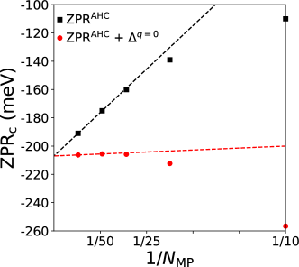
Figure S1: The ZPR${}^{\rm AHC}_{\rm c}$ of MgO is computed without correction (black squares), and then with correction Eq. (14) (red circles), for different phonon wavevector Monkhorst-Pack $\mathbf{q}$-grid samplings, characterized by $N_{\rm MP}$. The points correspond to $N_{\rm MP}=96,48,32,20$ and $10$. Dotted lines show linear extrapolation with respect to $1/N_{\rm MP}$ from the $N_{\rm MP}=48$ and $N_{\rm MP}=96$ grids, to the infinitely large $N_{\rm MP}$ value.

II Band gap zero-point renormalization from experiment and from the theoretical approaches (AHC and ASC)

Table S2 compares ZPR_g data from experiment and from different computations. These data are used in Fig. 2 of the main text. Further computed ZPR_g data are provided in Table S3, although the latter focuses on band gaps, to be analyzed in the next section (Sec. III). Gathering experimental ZPR_g data needed some care, as explained below. Also, theoretical data ought to be discussed in view of previous works. For the in-depth discussion of the theoretical data among themselves, we refer to Sec. V. We also complete the list of references in which ZPR_g have been computed, that had been mentioned in the main text.

Table S2: For eighteen materials: experimental fundamental gap and type (d=direct, i=indirect); experimental zero-point renormalization of the gap; lattice contribution to the zero-point renormalization of the gap; first-principles AHC zero-point renormalization of the gap; ratio $R$ between sum of AHC and lattice values and experimental values (see text) (ZPR${}^{\rm AHC}_{\rm g}$+ZPR${}^{\rm lat}_{\rm g}$)/ZPR${}^{\rm exp}_{\rm g}$; first-principles ASC zero-point renormalization of the gap. Experimental ZPR${}^{\rm exp}_{\rm g}$ data are obtained from extrapolation of temperature dependence of the gap, or isotopic mass derivatives of the gap. The latter are indicated with an asterisk. For SiC, the experimental data refer to the 15R polymorph, while the theoretical data refer to the 3C (zb) polymorph. They have similar sp³ topology, but differ by stacking sequence. For SrTiO₃, the ZPR${}^{\rm lat}_{\rm g}$ was hardly computable with the TDep methodology presented in the METHODS section of the main text. We have estimated it combining experimental data for the zero-point correction to the volume Lytle (1964) and theoretical data for the derivative of the gap with volume Zacharias, Scheffler, and Carbogno (2020), see text. The reference experimental value for AlN is the average of the reported values from Refs. Pässler, 2002 and Pässler, 2003, see text.

	$E_{\rm g}$	ZPRg	ZPR${}_{\rm g}^{\rm lat}$	ZPRg	$R$	ZPRg
	exp	exp		AHC		ASC
				present		PBE
	[not, d]			work		[Karsai et al., 2018]
Material	(eV)	(meV)	(meV)	(meV)		(meV)
Ge-dia	0.74 (i)	-52 [Parks et al., 1994]*	-10	-33	0.83	-50
		-52 [Pässler, 2002]
Si-dia	1.17 (i)	-59 [Karaiskaj et al., 2002]*	+9	-56	0.80	-65
		-72 [Pässler, 2002]
GaAs-zb	1.52 (d)	-60 [Pässler, 2002]	-29	-18	0.78	-53
CdTe-zb	1.61 (d)	-16 [Pässler, 2002]	-8	-20	1/0.57	-15
AlSb-zb	1.69 (i)	-35 [Pässler, 2002]	+6	-51	0.78	-43
CdSe-zb	1.85 (d)	-38 [Pässler, 2002]	-7	-34	1/0.93	-21
AlAs-zb	2.23 (i)	-50 [Pässler, 2002]	+8	-74	1/0.76	-63
GaP-zb	2.34 (i)	-85 [Pässler, 2002]	+8	-65	0.67	-57
ZnTe-zb	2.39 (d)	-40 [Pässler, 2002]	-18	-22	1.00	-24
SiC	2.40 (i)	-215 [Pässler, 2002]	+6	-179	0.80	-109
CdS-zb	2.58 (d)	-62 [Zhang et al., 1998]*	-10	-70	1/0.78	-29
		-34 [Pässler, 2002]
ZnSe-zb	2.82 (d)	-55 [Pässler, 2002]	-17	-44	1/0.90	-28
ZnS-zb	3.84 (d)	-105 [Manjon et al., 2005]*	-24	-88	1/0.94	-44
		-78 [Pässler, 2002]
C-dia	5.48 (i)	-338 [Collins et al., 1990]*	-27	-330	1/0.95	-320
		-334 [Pässler, 2002]
SrTiO3	3.25 (i) [Benrekia et al., 2012]	-336 [Kok et al., 2015]	$\approx$ +20	-290	0.80
ZnO-w	3.44 (d)	-164 [Manjon et al., 2003]*	-17	-157	1/0.94	-57
GaN-w	3.47 (d)	-180 [Pässler, 2002]	-49	-189	1/0.75	-94
AlN-w	6.20 (d)	-417	-85	-399	1/0.88
		-350 [Pässler, 2002]
		-483 [Pässler, 2003]

Table S3: Electronic gaps and corrections due to the zero-point motion (ZPR${}^{\rm AHC}_{\rm g}$ and ZPR${}^{\rm lat}_{\rm g}$), for thirteen materials: one-shot GW calculation of E_g, without ZPR (E${}^{\rm G_{0}W_{0}}_{\rm g}$); self-consistent GW with electron-hole corrections ($E^{\rm GWeh}_{\rm g}$) which is the best theoretical $E_{\rm g}$ without ZPR ; first-principles ZPR${}^{\rm AHC}_{\rm g}$ and firs-principles ZPR${}^{\rm lat}_{\rm g}$ (this work); ZPR-corrected $E^{\rm GWeh}_{\rm g}$ ($E^{\rm+ZPR}_{\rm g}$), namely $E^{\rm+ZPR}_{\rm g}$=$E^{\rm GWeh}_{\rm g}$+ZPR${}^{\rm AHC}_{\rm g}$+ZPR${}^{\rm lat}_{\rm g}$ ; experimental gap ($E^{\rm exp}_{\rm g}$). The ratios between $E^{\rm G_{0}W_{0}}_{\rm g}$ and $E^{\rm exp}_{\rm g}$, between $E^{\rm GWeh}_{\rm g}$ and $E^{\rm exp}_{\rm g}$, between $E^{\rm GWeh}_{\rm g}$+ZPR${}^{\rm AHC}_{\rm g}$ and $E^{\rm exp}_{\rm g}$ and between $E^{\rm+ZPR}_{\rm g}$ and $E^{\rm exp}_{\rm g}$, are shown in Fig. 3, but not reported here. Then, the ratio $R^{\rm ZPR}_{\rm GWeh}$ between ZPR${}_{\rm g}^{\rm AHC+lat}$ and the correction brought by the scGWeh approximation $E^{\rm GWeh}_{\rm g}$ with respect to $E^{\rm G_{0}W_{0}}_{\rm g}$, is mentioned. The values for $E^{\rm G_{0}W_{0}}_{\rm g}$ are taken from Ref. Shishkin and Kresse, 2007, except for Ge-dia, that comes from Ref. van Setten et al., 2017.

	$E^{\rm G_{0}W_{0}}_{\rm g}$	$E^{\rm GWeh}_{\rm g}$	ZPR${}^{\rm AHC}_{\rm g}$	ZPR${}^{\rm lat}_{\rm g}$	$E^{\rm+ZPR}_{\rm g}$	$E^{\rm exp}_{\rm g}$	$R^{\rm ZPR}_{\rm GWeh}$
	[Shishkin and Kresse, 2007,van Setten et al., 2017]	[Shishkin, Marsman, and Kresse, 2007]			[not, d]
Material	eV	eV	eV	eV	eV	eV
Ge-dia	0.53	0.81	-0.033	-0.010	0.77	0.74	-0.15
Si-dia	1.12	1.24	-0.056	0.009	1.19	1.17	-0.39
GaAs-zb	1.30	1.62	-0.024	-0.029	1.57	1.52	-0.17
SiC-zb	2.27	2.53	-0.179	0.006	2.36	2.40	-0.67
CdS-zb	2.06	2.39	-0.070	-0.010	2.31	2.42	-0.24
AlP-zb	2.44	2.57	-0.093	0.010	2.49	2.45	-0.64
GaN-w	2.80	3.27	-0.189	-0.049	3.03	3.20	-0.51
ZnO-w	2.12	3.20	-0.157	-0.017	3.03	3.44	-0.16
ZnS-zb	3.29	3.60	-0.088	-0.024	3.49	3.91	-0.36
C-dia	5.50	5.79	-0.330	-0.027	5.43	5.48	-1.23
BN-zb	6.10	6.59	-0.406	-0.017	6.17	6.25	-0.86
MgO-rs	7.25	8.12	-0.524	-0.117	7.48	7.67	-0.74

II.1 Experimental data: discussion

As explained by Cardona and Thewalt, in relation to the Table 3 of their review Ref. Cardona and Thewalt, 2005, the experimental ZPR are obtained by two different techniques. The first one starts from measurements of the band gap energy for different samples of a material with varying isotopic content. The derivative(s) of the band gap with respect to the mass(es) are extracted, followed by extrapolation to infinite mass(es). The second one relies on measurements of the band gap energy in a large temperature range, including the low-temperature regime, but also the high-temperature regime, where a linear asymptote must be reached. In this case, the ZPR is the difference between the measured zero-temperature limit and the linear extrapolation of the high-temperature asymptote to zero temperature, as shown for Ge in Fig. 21 of Ref. Cardona and Thewalt, 2005. When both techniques agree, the experimental result can be reasonably trusted.

For the latter technique (extrapolation of temperature-dependent data), we rely on the analysis of PässlerPässler (2002, 2003), that superceeds his earlier workPässler (1999) on which Ref. Cardona and Thewalt, 2005 relied. The two publications by PässlerPässler (2002, 2003) yield essentially equivalent results, except for AlN. For this material, we have taken the mean of the two reported values as reference. However, also in the latter case, our results are within the 25% limit. We have surveyed the literature after 2003, but were unable to find more reliable data.

For the isotopic extrapolation, to our surprise, a large fraction of the data provided in the related column of Table 3 of Ref. Cardona and Thewalt, 2005 do NOT report actual isotopic extrapolation analysis. We have thus extensively examined the primary literature, and have obtained that such isotopic extrapolation is available reliably for the following materials in our list: Ge, Si, C, CdS, ZnO and ZnS. They are clearly identified as such in table S2. Moreover, we have also realized that a non-negligible number of data available through other secondary references are misleading. We will not elaborate further on this problem, but generally speaking, we warn the reader about the unreliability of several publications in the field. The above-mentioned works of Pässler are apparently free of such problem.

Anyhow, the two techniques agree very well for Ge or C, or reasonably (within 25%) for Si and ZnS, but clearly differ for CdS (about a factor of 2). PässlerPässler (2002) does not provide data for ZnO. In Fig.2 of the main text, we have taken the isotopic extrapolation result as reference, since the extrapolation of temperature-dependent data is often plagued with insufficient sampling of the high-temperature region, which is crucial for the correct extrapolation, as discussed at length in Ref. Pässler, 1999. For the above-mentioned CdS discrepancy, the global expected trend due to the change of mass, comparing with CdSe and CdTe, or with the Zn series, appears more reasonable from the isotopic technique than from extrapolation of temperature-dependent data. Also, the comparison of the different analyses by Pässler, in 1999, 2002, and 2003, Refs. Pässler, 1999, 2002, 2003, shows stability for a few materials, but, more generally, non-negligible variations, at the 10-25% level. On this basis, one can infer that, globally speaking, the reliability of the experimental data is on the order of 25%, which is the reason of our use of this value in the main text.

Note that Karsai et al. Karsai et al. (2018) quotes experimental data (most from secondary sources) for about half the materials they compute, but miss many available data, especially those that do not compare well with their results.

II.2 Theoretical AHC data: discussion

The values quoted in Tables S2 and S3 for the band gap ZPR of C, BN, and MgO, respectively -330 meV, -406 meV, and -524 meV, differ from those previously published in Ref. Antonius et al., 2015, authored by some of us, giving respectively -366 meV, -370 meV, and -341 meV. We emphasize that the same first-principles method as in our current manuscript (non-adiabatic AHC) was used to obtain these data. The differences with the present data are entirely due to the sampling of the Brillouin Zone and associated imaginary broadening factor.

In Ref. Antonius et al., 2015, the sampling of the Brillouin Zone was already emphasized as an important technical issue, especially considering the numerical noise. For the purpose of computing the self-energy (which was the focus of Sec. II of Ref. Antonius et al., 2015), or computing the importance of “anharmonic effects” in the adiabatic approximation (Sec. III of Ref. Antonius et al., 2015), such numerical noise was addressed by keeping a large finite imaginary broadening (between 0.1-0.4 eV) and a fixed wavevector sampling 32x32x32. The choice of the value of the imaginary broadening was detailed in the Appendix of this paper, which was explicitly mentioned in the caption of this Table 1: “See Appendix for the values of the $\eta$ parameters used". Such imaginary broadening was determined to ensure removal of the noise in the self-energy, in order to produce Fig. 1 and 2, but however did not deliver an accurate absolute value for the ZPR in Table I of Sec. II.

Indeed, in another publication of some of ours (even slightly before Ref. Antonius et al., 2015), namely Ref. Poncé et al., 2015, the proper limit of vanishing imaginary broadening with much improved wavevector sampling was performed, for C and BN (up to 125x125x125 grid). The same values for C and BN as mentioned in our current manuscript, namely -330 meV and -406 meV, were found (with one more digit, see Table VII, column “Non-adiabatic"). MgO was not examined in Ref. Poncé et al., 2015, but the MgO band gap ZPR was then mentioned in Ref. Nery et al., 2018, still another publication from some of ours, page 11, end of second paragraph of first column, 526 meV. Such value is very similar to the values in our manuscript. The extrapolation scheme, differing from the one chosen in the present paper, explains the difference of 2 meV for MgO. The analysis of LiF is not done in the current work because an estimate of the Fröhlich parameter for the valence bands yields $\alpha$ bigger than 8, see Ref. Nery et al., 2018, which is beyond the validity of the present perturbative treatment. By the way, the top of the valence band does not occur at $\Gamma$ (see e.g. Ref. Persson et al., 2018, which was not mentioned in Ref. Nery et al., 2018).

II.3 Modification of the ZPR due to lattice parameter changes

The ZPR${}^{\rm AHC}_{\rm g}$ is computed at the fixed theoretical lattice parameters and internal coordinates minimizing the DFT energy (or fixed experimental lattice parameters in the case of Ge, GaAs and TiO₂). The phonon population effects on the lattice parameters, and induced change of band gap, are not taken into account in such procedure. This corresponds strictly to the harmonic approximation.

In the so-called quasi-harmonic approximation, the equilibrium lattice parameters and possibly internal coordinates are relaxed in order to minimize the free energy of the system. This makes such parameters depend on the temperature (thermal expansion), but also induces their zero-point change at $T=0$ K. In turn, such changes modifies the gap, an effect to be accounted for in order to compare with the experimental ZPR_g. This effect has been investigated by Garro and coworkers, Ref. Garro et al., 1996. It is also included in several first-principles calculations of the ZPR, see e.g. Ref. Villegas, Rocha, and Marini, 2016a.

In the present work, we have indeed added this effect beyond the harmonic approximation: we have computed the equilibrium lattice parameters with and without zero-point motion, then evaluated the change of gap. In the first case, we have minimized the Born-Oppenheimer energy without phonon contribution, giving $\{{\bf{R}}_{i}^{fix}\}$. In the second case, the free energy, including zero-point phonon contributions computed at different lattice parameters and interpolated between them, was minimized, giving $\{{\bf{R}}_{i}^{T=0}\}$. This procedure is similar to the one described in Ref. Rignanese, Michenaud, and Gonze, 1996, albeit extended to two dimensions (uniaxial and basal lattice parameters) in the case of wurtzite materials. The differences in band gap values for such lattice parameters form the lattice ZPR modification of the electronic structure:

$${\rm ZPR}_{\mathbf{k}n}^{\rm lat}={\rm\varepsilon}_{\mathbf{k}n}(\{{\bf{R}}_{i}^{T=0}\})-{\rm\varepsilon}_{\mathbf{k}n}(\{{\bf{R}}_{i}^{fix}\}).$$ (16)

In such approach, one supposes that there is no cross-influence of the modification of lattice parameters on the AHC ZPR. Also, one relies on the approximation that the internal parameters, if not determined by symmetry, are those that minimize the Born-Oppenheimer energy at the corresponding ${\bf{R}}_{i}$ lattice parameters. In other words, the deviatoric thermal forces and their effect on the band gap are not included, but the deviatoric thermal stresses are taken into account, following Ref. Carrier, Wentzcovitch, and Tsuchiya, 2007. In the list of materials of Tables S2 and S3, deviatoric thermal forces only appear for wurtzite materials, that have a quite symmetric tetrahedral environment, and thus, very small expected effect.

II.4 A survey of zero-point renormalization computations

In complement to the references given in the introduction of the main text, we list additional ones in view of further comparisons, without pretending to be exhaustive. Refs.  Marini, 2008; Giustino, Louie, and Cohen, 2010; Cannuccia and Marini, 2011; Gonze, Boulanger, and Côté, 2011; Cannuccia and Marini, 2012; Kawai et al., 2014; Poncé et al., 2014a, b; Antonius et al., 2015; Friedrich et al., 2015; Poncé et al., 2015; Villegas, Rocha, and Marini, 2016a; Nery and Allen, 2016; Saidi, Poncé, and Monserrat, 2016; Molina-Sanchez et al., 2016; Antonius and Louie, 2016; Villegas, Rocha, and Marini, 2016b; Nery et al., 2018; Ziaei and Bredow, 2017; Tutchton, Marchbanks, and Wu, 2018; Cao et al., 2019; Querales-Flores et al., 2019, 2020; Lihm and Park, 2020 report calculations of the ZPR_g based on the AHC approach with KS-DFT wavefunctions and eigenenergies. Refs. Capaz et al., 2005; Gonze, Boulanger, and Côté, 2011; Han and Bester, 2013; Patrick and Giustino, 2013; Monserrat, Drummond, and Needs, 2013; Antonius et al., 2014; Monserrat et al., 2014; Monserrat and Needs, 2014; Monserrat, Engel, and Needs, 2015; Patrick, Jacobsen, and Thygesen, 2015; Zacharias, Patrick, and Giustino, 2015; Engel, Monserrat, and Needs, 2015; Monserrat, 2016a; Zacharias and Giustino, 2016; Saidi, Poncé, and Monserrat, 2016; Karsai et al., 2018; Monserrat, 2018; Bravic and Monserrat, 2019 report calculations of the ZPR_g based on the ASC approach, usually based on KS-DFT, but also sometimes based on GW, see Refs. Antonius et al., 2014; Monserrat, 2016a; Karsai et al., 2018. As analyzed by the present generalized Fröhlich model, the ASC might be reasonably predictive for purely covalent materials (e.g. C, Si, Ge), or weakly infrared-active ones (e.g. GaAs), however, when the ZPR^gFr is a significant fraction of the ZPR, the predictive capability of the ASC approaches should be questioned. Even in the covalent case, non-adiabatic corrections can be sizeable (5…15%), see Table VII of Ref. Poncé et al., 2015. The ASC GW calculations performed until now Antonius et al. (2014); Monserrat (2016a); Karsai et al. (2018) rely at most on 4x4x4 supercells, which is at the limit of convergence. Going from 4x4x4 to 5x5x5 supercells for KS-DFT indeed still brings some modification, as shown by Ref. Karsai et al., 2018. For this reason, the effect of relying on GW corrections can hardly be clarified in the present context, which focuses on the non-adiabatic effects.

In a very recent publication Engel et al. (2020), Engel and coworkers have proposed a new method to compute the ZPR, combining supercell calculations with an interpolation method, still in the adiabatic approximation. They applied it for 9 materials, a subset of those examined by Karsai and coworkers Karsai et al. (2018) (focusing only on covalent or weakly ionic materials). The results that they obtain do not change the overall assessment of the adiabatic approach that we present here: for some materials, the agreement with experiment is slightly improved or deteriorated.

Studies of strongly infrared-active materials using the ASC include e.g. hydrogen-containing materials HF, H₂O, NH₃ and CH₄ in Ref. Monserrat, Engel, and Needs, 2015, where a giant electron-phonon interaction in molecular crystal and related important nonquadratic coupling had been investigated, the study of ice in Ref. Engel, Monserrat, and Needs, 2015, and the study of LiF, MgO and TiO₂ in Ref. Monserrat, 2016a, and some of the results from Ref. Karsai et al., 2018 for IR-active materials.

In addition to these references, the electron-phonon interaction has been directly incorporated in GW calculations in Refs. Botti and Marques, 2013; Lambrecht, Bhandari, and van Schilfgaarde, 2017; Bhandari et al., 2018. These are further commented upon in the next section.

Table S4 presents KS-DFT ASC data that were not reported in Table S2, as the latter only mentioned such data from Ref. Karsai et al., 2018. This table S4 still focuses on our set of materials, for which AHC data are available. For the indirect gap of Si and of SiC, as well as both the direct and indirect gaps of C, the different ASC calculations agree very well. The agreement is less good for GaAs and the direct gap of Si. Anyhow, these data confirm that AHC and ASC calculations of the fundamental band gap reasonably agree for covalent materials, but strongly disagree for strongly IR-active materials (SiC-zb, TiO₂-t, MgO-rs).

Table S4: Experimental fundamental gap E${}_{\rm g}^{\rm exp}$ and type (d=direct, i=indirect), first-principles zero-point renormalization of the gap ZPR${}^{\rm AHC}_{\rm g}$: from the AHC (present work), and from the ASC.

	Eg	ZPRg	ZPRg
	exp	AHC	ASC
		present	KS-DFT
	[not, d]	work
Material	(eV)	(meV)	(meV)
Si-dia	1.17 (i)	-56	-60 [Monserrat and Needs, 2014]
			-57 [Zacharias and Giustino, 2016]
			-65 [Karsai et al., 2018]
			-75 [Zhang et al., 2020]
	3.40 (d)	-42	$\approx$ -28 [Monserrat, 2016a]
			-44 [Zacharias and Giustino, 2016]
GaAs-zb	1.52 (d)	-18	-23 [Antonius et al., 2014]
			-32 [Zacharias and Giustino, 2016]
			-53 [Karsai et al., 2018]
SiC	2.40 (i)	-179	-109 [Monserrat and Needs, 2014]
			-109 [Karsai et al., 2018]
			-145 [Zhang et al., 2020]
TiO2-t	3.03 (d)	-337	$\approx$ -150 [Monserrat, 2016a]
C-dia	5.48 (i)	-330	-334 [Monserrat and Needs, 2014]
			-345 [Zacharias and Giustino, 2016]
			-320 [Karsai et al., 2018]
			-437 [Zhang et al., 2020]
	7.07 (d)	-416	-437 [Antonius et al., 2014]
			$\approx$ -410 [Monserrat, 2016a]
			-450 [Zacharias and Giustino, 2016]
MgO-rs	7.67 (i)	-524	$\approx$ -220 [Monserrat, 2016a]
			-281 [Zhang et al., 2020]

III Gap values from experiment and different computations

Table S3 compares gap values from experiment and from different computations. These data are used in Fig. 3. The set of 12 materials in this table includes all those for which self-consistent GW calculations with electron-hole corrections have been performed in Ref. Shishkin, Marsman, and Kresse, 2007, except Ne, LiF and Ar. We did not include them in our study for the following reasons. Ne and Ar are strongly affected by weak van der Waals interactions. Much more than the other materials, they will be modified by the zero-point lattice corrections, discussed earlier. For LiF, as mentioned previously, the estimated value of $\alpha$ show that the present perturbative treatment is likely invalid. For all three materials, excitonic effects are strong, and should likely be included for meaningful comparison with experimental data.

Suppplementary Table III quotes E${}^{\rm G_{0}W_{0}}_{\rm g}$ values from Ref. Shishkin and Kresse, 2007, except for Ge-dia, that comes from Ref. van Setten et al., 2017. The latter reference also presents E${}^{\rm G_{0}W_{0}}_{\rm g}$ values for many materials, including more than half of those reported in Table S3. Many other E${}^{\rm G_{0}W_{0}}_{\rm g}$ values for those materials have been published. The spread in such values for one material can be as large as 0.5 eV. A comparative study of published E${}^{\rm G_{0}W_{0}}_{\rm g}$ values is out-of-scope of the present publication, but is presented in Ref. Rangel et al., 2020. The values E${}^{\rm G_{0}W_{0}}_{\rm g}$ in Table S3 have the goal to show the typical size of the E${}^{\rm G_{0}W_{0}}_{\rm g}$ to E${}^{\rm GWeh}_{\rm g}$ correction, and point out that the ZPR correction is of the same order of magnitude for materials with light nuclei.

In addition to the AHC and ASC methodologies, there has also been attempts to incorporate directly the electron-phonon interaction inside the GW approach Botti and Marques (2013); Lambrecht, Bhandari, and van Schilfgaarde (2017); Bhandari et al. (2018) to obtain modified gap values or ZPR_g. The first publication on the subject, by Botti and Marques Botti and Marques (2013) was later shown by Lambrecht, Bhandari and van Schilfgaarde Lambrecht, Bhandari, and van Schilfgaarde (2017) to ignore the range of the Fröhlich interaction, yielding an erroneous integration over the Brillouin Zone. Even in the latter work, there is a factor of 2 difference for the Fröhlich $\alpha$ compared to the usual definition, used in the present work. Their ZPR_g results (Table I of Ref. Lambrecht, Bhandari, and van Schilfgaarde, 2017 and Bhandari et al., 2018) for MgO, GaN-zb and SrTiO₃, resp. (-219 meV, -67 meV, -404 meV) can be compared with ours (-517 meV, -171 meV, -290 meV), see Table S5. They very clearly differ, with strong underestimation with respect to ours for MgO, GaN-zb, and strong overestimation for SrTiO₃. For SrTiO₃, our results agree better with the experimental data (-336 meV), see Table S2. For MgO and GaN-zb, a direct measurement of ZPR_g is not available. Still, experimental value for the other polymorph of GaN, namely GaN-w (-180 meV) is reported in Table S2 and matches very well our ZPR${}^{\rm AHC}_{\rm g}$ value (-189 meV) for GaN-w.

IV From the adiabatic AHC approach to the generalized Fröhlich Hamiltonian

In order to help understand why the generalized Fröhlich Hamiltonian captures correctly the physics of the Fan diagram, at variance with the adiabatic approximation, we summarize first the discussion of the AHC case given in Ref. Poncé et al., 2015. Then, we derive the generalized Fröhlich Hamiltonian from Eq. (8) of the main text.

IV.1 The divergence of the adiabatic AHC for IR-active materials

Under the adiabatic approximation, the phonon frequencies $\omega_{\textbf{q}j}$ are neglected when compared to differences between electronic eigenenergies. In other words, one supposes that the electron (or hole) responds instantaneously to the atomic vibrations, even for those electronic transitions with a characteristic time scale (inversely proportional to the eigenenergy difference) larger than the phonon oscillation period. This simplification is of course questionable for intraband transitions with small momentum transfer, as shown in Ref. Poncé et al., 2015. Suppressing $\omega_{\textbf{q}j}$ in the denominators of Eq. (8) , and evaluating the AHC ZPR according to Eqs. (7) and (9) yields

$${\rm ZPR}^{\rm adiab}_{\mathbf{k}n}= \Re e\frac{1}{N_{\mathbf{q}}}\sum_{\mathbf{q}j}^{\rm BZ}\sum_{n^{\prime}}\frac{|\langle\mathbf{k+q}n|H^{(1)}_{\mathbf{q}j}|\mathbf{k}n^{\prime}\rangle|^{2}}{\varepsilon_{\mathbf{k}n}-\varepsilon_{\mathbf{k+q}n^{\prime}}+i\eta}+\Sigma^{\mathrm{DW}}_{\mathbf{k}n}.$$

For band edges, in particular the top of the valence band or the bottom of the conduction band, and considering at present non-degenerate bands, the intraband ($n^{\prime}=n$) contribution when $\eta=0$ has two different types of divergences for $q\rightarrow 0$, reinforcing each others: (i) for IR-active materials, the electron-phonon interaction matrix elements of $H^{(1)}_{\mathbf{q}j}$ diverge like $\delta_{nn^{\prime}}/q$, while (ii) the denominator behaves like $q^{2}/2m^{*}_{\hat{\mathbf{q}}}$. In these expressions, $q$ is the norm of the $\mathbf{q}$ wavevector, and $m^{*}_{\hat{\mathbf{q}}}$ is the effective mass along direction $\mathbf{q}$, represented by the unit vector $\hat{\mathbf{q}}$, with $\mathbf{q}=q\cdot\hat{\mathbf{q}}$. The effective mass is the inverse of the second derivative of the eigenenergy with respect to the wavevector along $\hat{\mathbf{q}}$ at the band extremum.

Thus, the integrand at small $q$ behaves like $1/q^{4}$. Focusing on the ZPR${}^{\rm adiab}_{\rm c}$ of the bottom of the conduction band (the handling of the top of the valence band is similar) one finds, in spherical coordinates, and introducing a spherical cut-off $q_{\rm c}$ whose limit $q_{\rm c}\rightarrow 0$ has to be taken:

$${\rm ZPR}^{\rm adiab}_{\rm c}(q_{\rm c}<q)=\int_{4\pi}\int_{q_{\rm c}}\frac{f^{\rm adiab}(q\hat{\mathbf{q}})}{q^{2}\big{(}\frac{q^{2}}{2m^{*}_{\hat{\mathbf{q}}}}+\mathcal{O}(q^{3})\big{)}}q^{2}dqd\hat{\mathbf{q}},$$ (18)

where $f^{\rm adiab}(q\hat{\mathbf{q}})$ is a smooth function of $q$ (it does not diverge, but also does not tend to zero for $q\rightarrow 0$). As announced Poncé et al. (2015), ${\rm ZPR}^{\rm adiab}_{\rm c}(q_{\rm c}<q)$ diverges like $1/q_{\rm c}$ when $q_{\rm c}\rightarrow 0$.

By contrast, if phonon frequencies are not suppressed in Eq. (8), which is the non-adiabatic case, one falls back to an integral of the type (here considered for one isotropic phonon branch only, and one non-degenerate isotropic electronic band):

$${\rm ZPR}^{\rm non-adiab}_{\rm c} (q_{\rm c}<q)=$$

$$\int_{4\pi}\int_{q_{\rm c}} \frac{f^{\rm non-adiab}(q\hat{\mathbf{q}})}{q^{2}\big{(}\frac{q^{2}}{2m^{*}_{\hat{\mathbf{q}}}}-\omega_{0}+\mathcal{O}(q^{2})\big{)}}q^{2}dqd\hat{\mathbf{q}},$$ (19)

where the $\mathcal{O}(q^{2})$ contribution in the denominator comes from the curvature of $\omega_{\textbf{q}}$ with respect to $q$, usually much smaller than the curvature of the electronic eigenenergies governed by $m^{*}_{\hat{\mathbf{q}}}$, explicitly mentioned in Eq. (19). ${\rm ZPR}^{\rm non-adiab}_{\rm c}(q_{\rm c}<q)$ does not diverge for $q_{\rm c}\rightarrow 0$, provided $\omega_{0}$ is non-zero.

Acoustic modes should not be forgotten. Their eigenfrequency $\omega_{0}$ tends to zero in the $q\rightarrow 0$ limit. However, the corresponding first-order electron-phonon matrix element does not diverge like $1/q$, and also, it has been shown by Allen and Heine Allen and Heine (1976) that, thanks to translational symmetry, the contribution to the Fan term from acoustic modes is exactly cancelled by the Debye-Waller term, in the $q\rightarrow 0$ limit. Thus no divergence arises from them.

To summarize, finite phonon frequencies at $q=0$ remove the AHC divergence in the non-adiabatic case.

IV.2 The generalized Fröhlich Hamiltonian

Instead of suppressing phonon frequencies appearing in the Fan self-energy Eq.(8), like in the adiabatic approximation, a radically different strategy is followed in the generalized Fröhlich Hamiltonian: one uses only parameters at $q=0$, including crucially the phonon frequencies, and extends them to the whole $\mathbf{q}$-space, using simple behavior for medium and large-$q$ (i.e. parabolic electronic dispersion and no phonon dispersion). This corresponds to macroscopic electrostatic treatment and a continuum space hypotheses.

The model proposed by Fröhlich Fröhlich (1954) in 1954 is the most simplified version of such hypotheses: one non-dispersive LO phonon branch, one electronic parabolic band governed by a single, isotropic effective mass, and electron-phonon interaction originating from the isotropic macroscopic dielectric interaction between the IR-active LO mode and the charged electronic carrier. No Debye-Waller contribution is included. Spin might be ignored, as only one electron is considered, without spin-phonon interaction. Explicitly, the Fröhlich Hamiltonian reads Fröhlich, Pelzer, and Zienau (1950); Fröhlich (1952, 1954); Feynman (1955),

$$\hat{H}^{\rm Fr}=\hat{H}^{\rm Fr}_{\rm el}+\hat{H}^{\rm Fr}_{\rm ph}+\hat{H}^{\rm Fr}_{\rm EPI}\,,$$ (20)

with

$$\hat{H}^{\rm Fr}_{\rm el}=\sum_{\mathbf{k}}\frac{\mathbf{k}^{2}}{2m^{*}}\hat{c}^{+}_{\mathbf{k}}\hat{c}_{\mathbf{k}}\,,$$ (21)

$$\hat{H}^{\rm Fr}_{\rm ph}=\sum_{\mathbf{q}}\omega_{\rm LO}\hat{a}^{+}_{\mathbf{q}}\hat{a}_{\mathbf{q}}\,,$$ (22)

$$\hat{H}^{\rm Fr}_{\rm EPI}=\sum_{\mathbf{q},\mathbf{k}}g^{\rm Fr}(\mathbf{q})\hat{c}^{+}_{\mathbf{k}+\mathbf{q}}\hat{c}_{\mathbf{k}}(\hat{a}_{\mathbf{q}}+\hat{a}^{+}_{-\mathbf{q}})\,,$$ (23)

where $\hat{a}^{+}_{\mathbf{q}}$ and $\hat{a}_{\mathbf{q}}$ are phonon creation and annihilation operators, $\hat{c}^{+}_{\mathbf{q}}$ and $\hat{c}_{\mathbf{q}}$ are electron creation and annihilation operators, and the electron-phonon coupling parameter is given by

$$g^{\rm Fr}(\mathbf{q})=\frac{i}{q}\Biggl{[}\frac{2\pi\omega_{\rm LO}}{V_{\rm BvK}}\Big{(}\frac{1}{\epsilon^{\infty}}-\frac{1}{\epsilon^{0}}\Big{)}\Biggr{]}^{1/2},$$ (24)

where $V_{\rm BvK}$ is the Born-von Karman normalisation volume corresponding to the $\mathbf{k}$ and $\mathbf{q}$ samplings, $q$ is the norm of $\mathbf{q}$ and $\hat{\mathbf{q}}$ is its direction, $\mathbf{q}=q\cdot\hat{\mathbf{q}}$, $\epsilon^{\infty}$ is the optical dielectric constant, and $\epsilon^{0}$ is the low-frequency dielectric constant. The sums over $\mathbf{k}$ and $\mathbf{q}$ run over the whole reciprocal space.

At the lowest order of perturbation theory, this yields the well-known result Fröhlich (1954); Feynman (1955); Mahan (2000) for the polaron binding energy (that we denote ZPR^Fr):

$${\rm ZPR}^{\rm Fr}=-\alpha\omega_{\rm LO},\,{\rm with}\,\alpha=\Big{(}\frac{1}{\epsilon^{\infty}}-\frac{1}{\epsilon^{0}}\Big{)}\sqrt{\frac{m^{\ast}}{2\omega_{\rm LO}}}.$$ (25)

Accurate diagrammatic Monte Carlo simulations Mishchenko et al. (2000) have demonstrated reasonable validity of this lowest-order perturbation result in a range that extends to about $\alpha\approx 8$. Beyond this, electronic self-trapping becomes too important, and the lowest-order result deviates strongly from the exact results.

Multiphonon generalisations of the Fröhlich model Hamiltonian have been considered in several occasions, but only in the cubic case, while the anisotropy of the electronic effective mass has been accounted for in an approximate way, and not altogether with the degeneracy of band edges, that has either been treated approximately, or for a spherical model, without warping, or only considering one phonon branch see e.g. Refs. Mahan, 1965; Trebin and Rössler, 1975; Devreese et al., 2010; Nery and Allen, 2016; Schlipf, Poncé, and Giustino, 2018; Bhandari et al., 2018.

Our generalized Fröhlich model includes all the features of real materials altogether: multiphonon, anisotropic, degenerate band extrema. It is derived by considering the full Eq. (8) and applying the same ansatz as the original Fröhlich model: we treat as exactly as possible the region in the Brillouin zone where the phonon frequency is large with respect to the eigenenergy differences, and, coherently, suppress the contributions from bands with a large energy difference with respect to phonon frequencies (interband contributions), keeping only intraband contributions. Like for the Fröhlich Hamiltonian, we use only parameters that describe the functions in the Brillouin zone around $q=0$, and extend them to the whole reciprocal space, using the same simple behaviors for medium and large-$q$: parabolic electronic dispersion and no phonon dispersion. We also retain only the macroscopic Fröhlich electron-phonon interaction, $\mathbf{G}=0$ component, following Vogl Vogl (1976). This is also coherent with the first-principles Fröhlich vertex of Ref. Verdi and Giustino, 2015, and the associated macroscopic electric field, derived in the appendix A of Poncé et al., Ref. Poncé et al., 2015. The possible degeneracy of the electronic states, causing the warping of the electronic structure, is addressed following Refs. Mecholsky et al., 2014 and  Laflamme Janssen et al., 2016. It has been shown also by AHC that the contribution to the Fan term from acoustic modes, for which the frequency vanishes when $q\rightarrow 0$, is exactly cancelled by the Debye-Waller term, close to $q=0$.

Having highlighted the basic ideas of the derivation of the generalized Fröhlich Hamiltonian, in what follows, we write down the mathematical expressions. We focus on the conduction band expression, ZPR_c, associated to one of the possibly degenerate states, labelled $c$, with energy $\varepsilon_{\rm c}$ and with wavevector $\mathbf{k}_{0}$. Similar expressions for ZPR_v can be derived. For the sake of simplicity, we will suppose that $\mathbf{k}_{0}$ is the Brillouin zone center $\Gamma$, but the equations that follow can be straightforwardly adapted to another value of $\mathbf{k}_{0}$. We also introduce $\mathbf{k}^{\prime}=\mathbf{k}+\mathbf{q}$.

Under the above hypotheses, the matrix elements of $H^{(1)}_{\mathbf{q}j}$ for $q\rightarrow 0$ writes

$$\langle\mathbf{k}^{\prime},n^{\prime}|H^{(1)}_{\mathbf{q}j}|\mathbf{k},n\rangle=\frac{i}{q} \frac{4\pi}{\Omega_{0}}\Big{(}\frac{1}{2\omega_{j0}(\hat{\mathbf{q}})V_{\rm BvK}}\Big{)}^{1/2}\frac{\hat{\mathbf{q}}.\mathbf{p}_{j}(\hat{\mathbf{q}})}{\epsilon^{\infty}(\hat{\mathbf{q}})}$$

$$\times \langle\mathbf{k}^{\prime},n^{\prime}|\mathbf{k},n\rangle_{\rm P}\,,$$ (26)

with $\Omega_{0}$ the primitive cell volume, $V_{\rm BvK}$ the Born-von-Karman normalisation volume corresponding to the $\mathbf{k}$ and $\mathbf{q}$ samplings, and the scalar product $\langle\mathbf{k}^{\prime},n^{\prime}|\mathbf{k},n\rangle_{\rm P}$ is computed from the periodic part of the Bloch functions. Sums over $\mathbf{k}$ and $\mathbf{q}$ of the type $\sum_{\mathbf{q}}f(\mathbf{q})/V_{\rm BvK}$ are to be replaced by $\Omega_{0}/(2\pi)^{3}\int d^{3}\mathbf{q}f(\mathbf{q})$ in the macroscopic limit in what follows. We have used the notation $\omega_{j0}(\hat{\mathbf{q}})$ for the $q\rightarrow 0$ limit of the $j$-phonon branch ($\omega_{j0}(\hat{\mathbf{q}})=\lim_{q\rightarrow 0}\omega_{j(q\hat{\mathbf{q}})}$), while the related mode-polarity vectors $\mathbf{p}_{j}(\hat{\mathbf{q}})$, see Eq. (41) of Ref. Veithen, Gonze, and Ghosez, 2005, are defined from the Born effective charges and the eigendisplacements of the phonon mode, summing over the atoms labelled by $\kappa$, and the Cartesian direction of displacement $\alpha$,

$$p_{\gamma,j}(\hat{\mathbf{q}})=\lim_{q\rightarrow 0}\sum_{\kappa\alpha}Z^{*}_{\kappa\alpha,\gamma}U_{\kappa\alpha,j}(q\hat{\mathbf{q}}).$$ (27)

Similarly, the optic dielectric constant along $\hat{\mathbf{q}}$ is obtained from the optic dielectric tensor by summing over wavevector components, $\epsilon^{\infty}(\hat{\mathbf{q}})=\sum_{\alpha\beta}\hat{q}_{\alpha}\epsilon^{\infty}_{\alpha\beta}\hat{q}_{\beta}$, as in Eq. (56) of Ref. Gonze and Lee, 1997. The mode-polarity vector vanishes for all non-IR-active modes. Thus naturally only the LO modes contribute to the ZPR^gFr in this generalized Fröhlich approach (for acoustic modes and TO modes, the mode-polarity vector vanishes). Still, the directional dependency of the phonon frequencies, of the mode-polarity vectors, and of the dielectric constant, is correctly taken into account.

We then restrict ourselves to the bands that are degenerate with $c$, and choose a $\hat{\mathbf{k}}$-independent complete basis for these states at $\mathbf{k}_{0}=\Gamma$, denoted $|\Gamma,m\rangle$. We also define the $\hat{\mathbf{k}}$-dependent overlap between states $m$ at $\Gamma$ and states $n$ along $\hat{\mathbf{k}}$ in the $k\rightarrow 0$ limit:

$$s_{nm}(\hat{\mathbf{k}})=\lim_{k\rightarrow 0}\langle k\hat{\mathbf{k}},n|\Gamma,m\rangle_{\rm P}\,.$$ (28)

This definition supposes that the phase of the $|k\hat{\mathbf{k}},n\rangle$ states is chosen continuously as a function of $k$, for vanishing $k$ along the $\hat{\mathbf{k}}$ direction. The phase can always be chosen to be continuous, and this choice will have no bearing on the results obtained later. Still, it does not imply any continuity hypothesis for the phase between states $n$ for different $\hat{\mathbf{k}}$ directions. The matrix $s_{nm}(\hat{\mathbf{k}})$ is unitary. Note that the $|\Gamma,m\rangle$ states are fixed before the $\hat{\mathbf{k}}$ direction is known. The coefficients $s_{nm}(\hat{\mathbf{k}})$ can be computed from first principles following the perturbative treatment of Refs. Mecholsky et al., 2014 and  Laflamme Janssen et al., 2016, which is the first-principles equivalent of the $\mathbf{k}.\mathbf{p}$ approach, restricted to the subspace spanned by the bands that connect to the degenerate states. It delivers Luttinger-Kohn parameters $D_{jj^{\prime}}^{\alpha\beta}$, Luttinger and Kohn (1955) that allows one to find $s_{nm}(\hat{\mathbf{k}})$ for all $\hat{\mathbf{k}}$. The Luttinger-Kohn parameters can also be determined from experimental measurements. The $s$ matrices can be thought as being the adaptation of spherical harmonics to the specific symmetry representation to which the degenerate wavefunctions belong.

With these definitions, we write the generalized Fröhlich electron-phonon interaction as

$$g^{\rm gFr}(\mathbf{q}j,\mathbf{k}n^{\prime}n)=\frac{i}{q} \frac{4\pi}{\Omega_{0}}\Big{(}\frac{1}{2\omega_{j0}(\hat{\mathbf{q}})V_{\rm BvK}}\Big{)}^{1/2}\frac{\hat{\mathbf{q}}.\mathbf{p}_{j}(\hat{\mathbf{q}})}{\epsilon^{\infty}(\hat{\mathbf{q}})}$$

$$\times \sum_{m}s_{n^{\prime}m}(\hat{\mathbf{k}}^{\prime})(s_{nm}(\hat{\mathbf{k}}))^{*}.$$ (29)

This expression depends on the directions $\hat{\mathbf{k}}$, $\hat{\mathbf{k}}^{\prime}$, and $\hat{\mathbf{q}}$, but not explicitly on their norm, except for the $\frac{1}{q}$ factor.

We focus then on the denominators appearing in the self-energy expression Eq. (8), evaluated at $\omega=\varepsilon_{\rm c}$, following Eq. (9). Again we consider only the intraband terms, for bands $n^{\prime}$ degenerate with $c$ in the $q\rightarrow 0$ limit. These bands, similarly to the $c$ state, are unoccupied, hence $f_{\mathbf{k}^{\prime}n^{\prime}}=0$. Thus the numerator of the second term in Eq. (8) vanishes. We find:

$$\lim_{q\rightarrow 0}(\varepsilon_{\rm c}-\varepsilon_{\mathbf{k}^{\prime}n^{\prime}}-\omega_{\mathbf{q}j}) = -\frac{q^{2}}{2m^{*}_{n^{\prime}}(\hat{\mathbf{k}}^{\prime})}-\omega_{j0}(\hat{\mathbf{q}}).$$ (30)

See Refs. Mecholsky et al., 2014 and  Laflamme Janssen et al., 2016 for the detailed treatment of $m^{*}_{n^{\prime}}(\hat{\mathbf{k}}^{\prime})$, the directional effective mass associated to one electronic band among a set of degenerate bands at an extremum.

Having clarified the electronic, phononic and electron-phonon interaction ingredients, we can write the corresponding Hamiltonian, Eqs.(1)-(5) that indeed generalizes properly Eqs. (20-24).

IV.3 Lowest-order perturbation treatment

Given the Hamiltonian, the lowest-order perturbation ZPR value can be inferred by integration over the radial $q$ coordinate. One obtains for the conduction bands:

$${\rm ZPR}_{\rm c}^{\rm gFr} = -\frac{1}{\pi\Omega_{0}}\int_{4\pi}d\hat{\mathbf{q}}\sum_{jn^{\prime}}\frac{|s_{n^{\prime}c}(\hat{\mathbf{q}})|^{2}}{2\omega_{j0}(\hat{\mathbf{q}})}$$ (31)

$$\times \Big{(}\frac{\hat{\mathbf{q}}.\mathbf{p}_{j}(\hat{\mathbf{q}})}{\epsilon^{\infty}(\hat{\mathbf{q}})}\Big{)}^{2}\Big{(}\frac{2m^{*}_{n^{\prime}}(\hat{\mathbf{q}})}{\omega_{j0}(\hat{\mathbf{q}})}\Big{)}^{1/2}\frac{\pi}{2}.$$

Let us denote by $n_{\rm deg}$ the degeneracy of the band edge. In the non-degenerate case ($n_{\rm deg}=1$), only $n^{\prime}={\rm c}$ has to be considered, then obviously $|s_{n^{\prime}{\rm c}}(\hat{\mathbf{q}})|=1$ independently of $\hat{\mathbf{q}}$. Grouping terms adequately, we obtain

$${\rm ZPR}_{\rm c}^{\rm gFr} = -\sum_{j}\frac{1}{\sqrt{2}\Omega_{0}}\int_{4\pi}d\hat{\mathbf{q}}\big{(}m_{\rm c}^{*}(\hat{\mathbf{q}})\big{)}^{1/2}$$ (32)

$$\times \big{(}\omega_{j0}(\hat{\mathbf{q}})\big{)}^{-3/2}\Big{(}\frac{\hat{\mathbf{q}}.\mathbf{p}_{j}(\hat{\mathbf{q}})}{\epsilon^{\infty}(\hat{\mathbf{q}})}\Big{)}^{2}.$$

The link can then be established with Eq. (25) in case of isotropic effective mass, isotropic dielectric tensor, and single LO phonon branch.

Let us further examine the degenerate case ($n_{\rm deg}>1$). We suppose that the degeneracy is not accidental, but due to symmetry reasons. In this case, we can exploit the symmetry to show that the computation $|s_{n^{\prime}{\rm c}}(\hat{\mathbf{q}})|^{2}$ can be avoided, as this factor can be replaced by $1/n_{\rm deg}$ in the integral. We will present the demonstration for the case of a three-fold degeneracy, that arises due to a cubic space group. This demonstration could be made general thanks to group theory.

At the bottom of the conduction band, located at the $\mathbf{k}_{0}$ wavevector, but that for convenience we again choose to be $\Gamma$, we set up a basis of three orthonormalized eigenfunctions, denoted $\{|X\rangle,|Y\rangle,|Z\rangle\}$, that form an irreducible representation of the symmetry group. The eigenfunction $|\Gamma,{\rm c}\rangle$ for which we compute the ZPR${}^{\rm gFr}_{\rm g}$, can be decomposed in this basis, with coefficients $(u_{{\rm c}X},u_{{\rm c}Y},u_{{\rm c}Z})$:

$$|\Gamma,{\rm c}\rangle=u_{{\rm c}X}|X\rangle+u_{{\rm c}Y}|Y\rangle+u_{{\rm c}Z}|Z\rangle.$$ (33)

The eigenfunctions $|q\hat{\mathbf{q}},n^{\prime}\rangle$ over which the $n^{\prime}$ sum and $\hat{\mathbf{q}}$ integral are done in Eq. (31) can be decomposed as well in this basis:

$$|q\hat{\mathbf{q}},n^{\prime}\rangle=s_{n^{\prime}X}(\hat{\mathbf{q}})|X\rangle+s_{n^{\prime}Y}(\hat{\mathbf{q}})|Y\rangle+s_{n^{\prime}Z}(\hat{\mathbf{q}})|Z\rangle$$

(34)

Thus Eq. (31) becomes

$${\rm ZPR}_{\rm c}^{\rm gFr}=\sum_{m\in\{X,Y,Z\}}\sum_{m^{\prime}\in\{X,Y,Z\}}u_{{\rm c}m}^{*}T_{mm^{\prime}}u_{{\rm c}m^{\prime}}$$ (35)

where

$$T_{mm^{\prime}}=-\sum_{jn^{\prime}}\frac{1}{\sqrt{2}\Omega_{0}} \int_{4\pi}d\hat{\mathbf{q}}s_{n^{\prime}m}(\hat{\mathbf{q}})s_{n^{\prime}m^{\prime}}^{*}(\hat{\mathbf{q}})\big{(}m_{n^{\prime}}^{*}(\hat{\mathbf{q}})\big{)}^{1/2}$$ (36)

$$\big{(}\omega_{j0}(\hat{\mathbf{q}})\big{)}^{-3/2}\Big{(}\frac{\hat{\mathbf{q}}.\mathbf{p}_{j}(\hat{\mathbf{q}})}{\epsilon^{\infty}(\hat{\mathbf{q}})}\Big{)}^{2}.$$

The second-rank tensor $T_{mm^{\prime}}$ does not depend on the state $c$. However the same ZPR${}^{\rm gFr}_{\rm c}$ must be obtained from Eq. (35) for any symmetrically equivalent state $c^{\prime}$. Hence, the tensor $T_{mm^{\prime}}$ must be invariant under all the symmetry operations of the group, which means

$$T_{mm^{\prime}}=t\delta_{mm^{\prime}},$$ (37)

where $\delta$ is the Kronecker symbol. $t$ can be evaluated thanks to the trace of $T_{mm^{\prime}}$,

$$n_{\rm deg}\cdot t= -\sum_{jn^{\prime}}\frac{1}{\sqrt{2}\Omega_{0}}\int_{4\pi}d\hat{\mathbf{q}}\Bigg{(}\sum_{m\in\{X,Y,Z\}}s_{n^{\prime}m}(\hat{\mathbf{q}})s_{n^{\prime}m}^{*}(\hat{\mathbf{q}})\Bigg{)}$$ (38)

$$\big{(}m_{n^{\prime}}^{*}(\hat{\mathbf{q}})\big{)}^{1/2}\big{(}\omega_{j0}(\hat{\mathbf{q}})\big{)}^{-3/2}\Big{(}\frac{\hat{\mathbf{q}}.\mathbf{p}_{j}(\hat{\mathbf{q}})}{\epsilon^{\infty}(\hat{\mathbf{q}})}\Big{)}^{2},$$

yielding

$${\rm ZPR}_{\rm c}^{\rm gFr} = -\sum_{jn}\frac{1}{\sqrt{2}\Omega_{0}n_{\rm deg}}\int_{4\pi}d\hat{\mathbf{q}}\big{(}m_{n}^{*}(\hat{\mathbf{q}})\big{)}^{1/2}$$ (39)

$$\times \big{(}\omega_{j0}(\hat{\mathbf{q}})\big{)}^{-3/2}\Big{(}\frac{\hat{\mathbf{q}}.\mathbf{p}_{j}(\hat{\mathbf{q}})}{\epsilon^{\infty}(\hat{\mathbf{q}})}\Big{)}^{2},$$

since $s_{nm}(\hat{\mathbf{k}})$ is unitary. Similar equations can be derived for the top of the valence band, yielding ${\rm ZPR}_{\rm v}^{\rm gFr}$.

IV.4 Generalized Fröhlich model with parameters from first-principles calculations

Table S5: For thirty materials: fundamental gap (E${}_{\rm g}^{\rm exp}$); location and possible degeneracy of the band edges (valence/conduction) from Ref.Persson et al., 2018 except for SrTiO₃; first-principles renormalization of the band edges (valence band maximum ZPR_v, conduction band minimum ZPR_c) and of the band gap (ZPR_g); and ratio between ZPR_g and E_g ($R_{\rm g}$). Methodology: “exp" for experimental results not (d), “gFr" for generalized Fröhlich model results, Eq. (37), and “AHC" for AHC first-principles results (with correction Eq. (3).

	Eg	Edge	ZPRv	ZPRv	ZPRc	ZPRc	ZPRg	$R_{\rm g}$
	exp	v/c	gFr	AHC	gFr	AHC	AHC	AHC
Material	eV	deg.	meV	meV	meV	meV	meV	%
Ge-dia	0.74	$\Gamma$/L	0	17	0	-16	-33	-4.5
Si-dia	1.17	$\Gamma$(3)/	0	35	0	-21	-56	-4.8
		X*(X-$\Gamma$)
GaAs-zb	1.52	$\Gamma$(3)/$\Gamma$	3	19	-1	1	-18	-1.2
CdTe-zb	1.61	$\Gamma$(3)/$\Gamma$	12	17	-4	-3	-20	-1.2
AlSb-zb	1.69	$\Gamma$(3)/	4	24	-4	-27	-51	-3.0
		X*(X-$\Gamma$)
CdSe-zb	1.85	$\Gamma$(3)/$\Gamma$	20	26	-6	-8	-34	-1.8
AlAs-zb	2.23	$\Gamma$(3)/X	12	39	-9	-35	-74	-3.3
GaP-zb	2.34	$\Gamma$(3)/	9	28	-7	-37	-65	2.8
		X*(X-$\Gamma$)
ZnTe-zb	2.39	$\Gamma$(3)/$\Gamma$	11	19	-4	-3	-22	-0.9
SiC-zb	2.40	$\Gamma$(3)/X	59	112	-32	-67	-179	-7.5
CdS-zb	2.42	$\Gamma$(3)/$\Gamma$	39	44	-15	-26	-70	-2.9
AlP-zb	2.45	$\Gamma$(3)/X	21	54	-14	-39	-93	-3.8
ZnSe-zb	2.82	$\Gamma$(3)/$\Gamma$	22	31	-8	-13	-44	-1.6
TiO2-t	3.03	$\Gamma$/$\Gamma$	236	195	-135	-142	-337	-11.1
SrTiO3	3.25	R(3) /	140	191	-115	-99	-290	-8.9
		$\Gamma$(3) Benrekia et al. (2012)
GaN-w	3.20	$\Gamma$/$\Gamma$	80	101	-31	-88	-189	-5.9
GaN-zb	3.29	$\Gamma$/$\Gamma$	77	85	-30	-91	-176	-5.3
ZnO-w	3.44	$\Gamma$/$\Gamma$	106	108	-38	-49	-157	-4.6
SnO2-t	3.73	$\Gamma$/$\Gamma$	144	176	-47	-39	-215	-5.8
ZnS-zb	3.91	$\Gamma$/$\Gamma$	40	49	-19	-39	-88	-2.3
BaO-rs	4.80	X/X	225	189	-133	-82	-271	-5.6
SrO-rs	5.22	$\Gamma$(3)/X	229	214	-141	-112	-326	-6.2
C-dia	5.48	$\Gamma$(3) /	0	134	0	-196	-330	-6.0
		X*(X-$\Gamma$)
AlN-w	6.20	$\Gamma$/$\Gamma$	151	204	-80	-195	-399	-6.4
BN-zb	6.25	$\Gamma$(3)/X	94	201	-68	-205	-406	-6.5
CaO-rs	6.93	$\Gamma$(3)/X	223	211	-154	-130	-341	-4.9
Li2O	7.55	$\Gamma$(3)/X	364	347	-172	-226	-573	-7.6
MgO-rs	7.83	$\Gamma$(3)/$\Gamma$	327	317	-137	-207	-524	-6.7
SiO2-t	8.90	$\Gamma$/$\Gamma$	292	300	-167	-285	-585	-6.6
BeO-w	10.59	$\Gamma$(2)/$\Gamma$	289	369	-191	-330	-699	-6.6

Table S5 presents the ZPR for the bottom of the conduction band and the top of the valence band from the present first-principles calculations: either based on the AHC approach, or from feeding the few relevant first-principles parameters in the generalized Fröhlich model. These data are used in Fig. 4.

Table S6: First-principles GGA-PBE parameters for the computation of the ZPR of band edges using the (generalized) Fröhlich model. Only materials with one IR-active phonon branch, cubic space group, and non-degenerate band extremum (though possibly anisotropic effective masses) are included in this table. For AlSb and GaP, the edge is located close to the X point, along the X-$\Gamma$ line, which is denoted X*.

	edge	$\epsilon^{\infty}$	$\epsilon^{0}$	$\omega_{\rm LO}$	$m^{*}_{xx}$	$m^{*}_{zz}$	$\alpha$	ZPRgFr
Material				(meV)	$m^{*}_{yy}$			(meV)
GaAs-zb	c $\Gamma$	15.31	17.55	33.5	0.009	0.009	0.016	-1
CdTe-zb	c $\Gamma$	8.89	12.37	19.1	0.052	0.052	0.192	-4
AlSb-zb	c X*	12.02	13.35	39.8	0.222	1.142	0.090	-4
CdSe-zb	c $\Gamma$	7.83	11.78	23.6	0.051	0.051	0.233	-6
AlAs-zb	c X	9.49	11.51	47.3	0.243	0.897	0.184	-9
GaP-zb	c X*	10.50	12.53	48.6	0.230	1.062	0.152	-7
ZnTe-zb	c $\Gamma$	9.05	11.99	24.1	0.076	0.076	0.178	-4
SiC-zb	c X	6.97	10.30	117.0	0.228	0.677	0.280	-32
CdS-zb	c $\Gamma$	6.21	10.24	34.4	0.118	0.118	0.432	-15
AlP-zb	c X	8.12	10.32	59.9	0.252	0.809	0.184	-14
ZnSe-zb	c $\Gamma$	7.35	10.73	29.3	0.089	0.089	0.276	-8
GaN-zb	c $\Gamma$	6.13	11.00	86.0	0.144	0.144	0.345	-30
ZnS-zb	c $\Gamma$	5.97	9.40	40.6	0.167	0.167	0.458	-19
BaO-rs	v X	4.21	92.43	47.3	4.035	0.431	4.757	225
BaO-rs	c X	4.21	92.43	47.3	0.380	1.197	2.812	-132
SrO-rs	c X	3.77	20.91	55.4	0.407	1.225	2.545	-141
BN-zb	c X	4.52	6.69	161.0	0.299	0.895	0.422	-68
CaO-rs	c X	3.77	16.76	66.8	0.443	1.424	2.305	-154
Li2O	c X	2.90	7.80	86.3	0.437	0.850	1.993	-172
MgO-rs	c $\Gamma$	3.23	11.14	84.5	0.340	0.340	1.624	-137

Table S6 presents the parameters computed from first principles, fed in the (generalized) Fröhlich model, only for materials with one phonon branch, with cubic symmetry and edges with non-degenerate electronic state, though including both isotropic or anisotropic effective masses. The parameters for other materials will be reported elsewhere. Most of such edges are found at the bottom of the conduction band, as most top of valence bands are degenerate. The information in Table VI allows one to compute the Fröhlich $\alpha$ parameter for these edges, ranging from 0.016 to 4.757. The lowest-order perturbation results are rather accurate in this range. A similar parameter to measure the breakdown of the perturbation theory in the case of degenerate electronic states is still to be established to our knowledge.

IV.5 Generalized Fröhlich model with parameters from experimental data

We discuss how a few-parameter Fröhlich Hamiltonian, of the type we have introduced, can be obtained from experimental data, thus constituting a few-parameter model of the ZPR of real materials.

In the Fröhlich model Fröhlich, Pelzer, and Zienau (1950); Fröhlich (1952, 1954); Feynman (1955) four parameters are needed: the LO phonon frequency $\omega_{\rm LO}$, the electronic dielectric constant $\epsilon^{\infty}$, the low-frequency dielectric constant $\epsilon^{0}$, and the effective mass $m^{\ast}$. These four parameters combine to give the $\alpha$ parameter mentioned in Eq. (24). The Fröhlich Hamiltonian can be expressed in the natural units of electronic effective mass and phonon frequency, to make appear $\alpha$ as the single parameter defining the Fröhlich Hamiltonian  Fröhlich, Pelzer, and Zienau (1950); Mahan (2000). Despite its simplicity, this Fröhlich Hamiltonian has resisted analytical treatments.

One can consider the generalization of such Fröhlich Hamiltonian to arbitrary electronic dispersion, phonon dispersion or electron-phonon interaction, as mentioned in the introduction of Ref. Devreese and Alexandrov, 2009. However, one has a model for a real material only if the parameters describing such dispersions and such interaction are available. Ideally, there should be as few parameters as possible if the goal is to extract the relevant physics.

In this respect, the Hamiltonian in Eqs. (1)-(5) is the proper generalization of Eqs. (19)-(23) to all band extrema (degenerate or not, isotropic or anisotropic) in all crystal types (cubic or not), because it can be parameterized with only a few numbers, and all such parameters can be found, in principle, from experiment, even if, in the present work, they were deduced from first principles.

Indeed, the electronic part, Eq. (2), is fully determined if the so-called Luttinger-Kohn parameters Luttinger and Kohn (1955) are available. Taking the example of the top of the valence band of a cubic material, with three-fold degeneracy, only three Luttinger-Kohn parameters, called $A$, $B$, and $C$ in Ref. Luttinger and Kohn, 1955 are needed to obtain the direction-dependent effective masses, $m^{*}_{n}(\hat{\mathbf{k}})$, of the three electronic bands, for all directions $\mathbf{k}$. Similarly, the direction-dependent phonon frequencies $\omega_{j0}(\hat{\mathbf{q}})$ and their mode-polarity vectors $p_{\gamma,j}(\hat{\mathbf{q}})$ can be obtained from neutron and infra-red spectra measurements and parametrized with a few numbers. For a cubic material with two atoms per unit cell, there is only one LO frequency, with mode-polarity vector directly determined from the LO-TO splitting. The optic dielectric constant along any direction $\mathbf{q}$ comes from the knowledge of a 3x3 symmetric tensor, easily obtained by optical measurements.

Conversely, in Ref. Verdi and Giustino, 2015, by Verdi and Giustino, a model for the electron-phonon interaction (or vertex) is proposed (at variance with our model of the full Hamiltonian, with a simplified vertex). It is used for a very different purpose. In this very nice study, Verdi and Giustino used the Fröhlich idea and the microscopic theory developed by Vogl Vogl (1976) to model the non-analytic behaviour of the electron-phonon vertex in the $\bf{q}\rightarrow 0$ limit. This approach was instrumental to make the electron-phonon interaction amenable to Fourier interpolation in an attempt to diminish the computational resources needed to capture the long-range behaviour of the scattering potentials and perform mobility calculations using Wannier functions. However, their work does not propose a ZPR model or Fröhlich Hamiltonian per se. Indeed, the electronic dispersion in Verdi and Giustino is the full first-principles dispersion in the entire Brillouin Zone and similarly for the phonon dispersion, unlike the one of the original Fröhlich approach (one parameter for each of these dispersions), and the present one, which relies on few parameters, the number of which depends on the crystal type and symmetries, and on the Luttinger-Kohn parameters.

V Zero-point renormalization in the ASC approach.

V.1 ASC Formalism and relation with the AHC

In the adiabatic supercell approach, the temperature-dependent average band edges (here written for the bottom of the conduction band) are obtained from

$$\langle\varepsilon_{\rm c}(T)\rangle=Z_{I}^{-1}\sum_{m}\exp(-\beta E_{m})\langle\varepsilon_{\rm c}\rangle_{m},$$ (40)

where $\beta=k_{B}T$ (with $k_{B}$ the Boltzmann constant), $T$ the temperature, $Z_{I}$ the canonical partition function among the quantum nuclear states $m$ with energies $E_{m}$ ($Z_{I}=\sum_{m}\exp(-\beta E_{m})$), and $\langle\varepsilon_{\rm c}\rangle_{m}$ the band edge average taken over the corresponding many-body nuclear wavefunction. See e.g. Eq. (4) of Ref. Monserrat, 2016b.

Such approach allows one to perform nonperturbative calculations, and thus includes effects beyond the adiabatic AHC approach, as emphasized in Sec.XI.A.2 of Ref. Giustino, 2017. It also allows one to use as starting point the GW eigenenergies, instead of the DFT ones, as proposed and used by some of us Antonius et al. (2014), and further exploited by Monserrat Monserrat (2016a) and Karsai et al. Karsai et al. (2018).

As detailed in Ref. Antonius et al., 2015, and illustrated in Fig. 4 of this reference, one can dissociate the harmonic approximation for the nuclear positions from the (non)quadratic behaviour of the eigenenergies as a function of the nuclear positions. While phonon anharmonicities can be safely ignored for most of the materials in the present context (except SrTiO₃, see the METHODS section of the main text, the (non)quadratic behaviour might very important in the ASC formalism. Within the harmonic approximation, one finds Eq. (19) of Ref. Antonius et al., 2015:

$$\langle\varepsilon_{\rm c}(T)\rangle=Z^{-1}_{I}\sum_{\bf n}\exp(-\beta E[{\bf n}])\int d{\bf z}|\chi_{\bf n}({\bf z})|^{2}\varepsilon_{\rm c}({\bf z}).$$

(41)

In this equation, $\bf z$ denotes the ensemble of all phonon coordinate amplitudes, while ${\bf n}$ denotes the ensemble of all phonon occupation numbers. As such, this expression does not diverge for IR-active materials, thanks to the sampling over coordinate amplitudes and the $\varepsilon_{\rm c}({\bf z})$ asymptotic linear behaviour, see Fig. 4 of Ref. Antonius et al., 2015 or Fig. 2 of Ref. Monserrat, Engel, and Needs, 2015. By contrast, making the quadratic approximation for the $\varepsilon_{\rm c}({\bf z})$ yields the AHC result for the Fan term, and hence, a divergence: the curvature becomes indeed infinite for IR-active longwavelength phonons. An extreme nonquadratic behavior is also observed in the degenerate case, as illustrated in Fig. 1 of Ref. Karsai et al., 2018. The connection with the adiabatic AHC result has been analyzed in detail in Ref. Poncé et al., 2014a.

However, obviously, Eq. (40) as well as Eq. (41) are based on the adiabatic approximation: the quantum nuclear state is not responding to the presence of an added or removed electron. Instead, Eq. (40) should have reflected such dependence to be correct. The correlation between electron and nuclei is not present in Eq. (40): the electron is affected by the phonons, but the phonons are incorrectly not affected by the addition of an electron. For IR-active materials, as explained in the main text, the lack of such correlation has important consequences for the predictive capability of the method.

As another consequence of the time-dependent atomic motion, the nonquadratic behaviour, present in the adiabatic treatment, looses its importance. The behaviour observed for degenerate electronic state, in the adiabatic approximation, exemplified by Fig. 1 of Ref. Karsai et al., 2018 might nevertheless still be relevant in the context of the Jahn-Teller effect. Anyhow, the transition between states, due to the first-order electron-phonon interaction, always involves a modification of the energy by the emission or absorption of a phonon. Hence, the corresponding initial and final energies are not identical.

V.2 The non-quadratic effect for IR-inactive materials

Coming back to the C-diamond case, the “anharmonic effect" in the adiabatic approximation is argued to be large in the above-mentioned Sec.III of Ref. Antonius et al., 2015, that some of us co-authored. At present, we call it more properly “non-quadratic effect” following Ref. Monserrat, Engel, and Needs, 2015. However, this study was performed within the adiabatic approximation. In the case of infrared active materials, without such “non-quadratic effects”, the ZPR is infinite in the adiabatic approximation. The non-quadratic effects succeed to bring the adiabatic ZPR to a finite value, i.e. it has “infinite” impact. For C, without such “non-quadratic effects”, the ZPR is finite in the adiabatic approximation, but nevertheless comes from the integration of a diverging integrand. Then the non-quadratic effects modify the adiabatic harmonic value by 40% by suppressing this diverging integrand. Still, despite yielding a finite value, the adiabatic approximation is incorrect to start with: if atomic motion effects are taken into account (and they should be taken into account from the very start, since the physics is the one of electrons not being able to follow the atomic motions), there is no diverging integrand that the non-quadratic effects would reduce afterwards. Thus, the crucial role of atom dynamics cannot be ignored even in diamond. We actually think that the estimation of non-quadratic effects in our publication Ref. Antonius et al., 2015 or in Ref. Monserrat, Engel, and Needs, 2015 cannot be transposed to the non-adiabatic treatment, even for the case of C. The non-quadratic effects in Ref. Antonius et al., 2015 or Ref. Monserrat, Engel, and Needs, 2015 remove a non-existing divergence, either global (IR-active materials), or integrable (non-IR-active materials), spuriously introduced by the adiabatic approximation.

V.3 GW approximation within the ASC: discussion

In such calculation of the ZPR of diamond, Ref. Antonius et al., 2014, we have obtained a 40% change of direct gap ZPR when the quantities needed in the ASC approach were obtained from GW instead of DFT. This effect appears to be comparable to the difference between AHC and experimental values reported in the present manuscript, while (as for the non-quadratic effect) C is an IR-inactive material.

In Ref. Karsai et al., 2018, a similar change was reproduced for the direct gap, but the change for the indirect (true) gap of diamond was much smaller, about 23%. For the other materials studied in Ref. Karsai et al., 2018, using the ASC approach, the ratio between GW and DFT, systematically obtained, was usually closer to unity, but not always. One can wonder whether such difference between GW and DFT would not also be obtained within the non-adiabatic AHC approach.

The estimation of such an effect within the non-adiabatic treatment is at present out of reach. Actually, as already argued in the previous sections, one can hardly justify transposing the conclusions obtained in the ASC approach to the non-adiabatic AHC approach, because the ASC approach relies on the non-quadratic coupling to eliminate the divergence of the ZPR, while for most materials, we believe such elimination to originate from the coupled dynamics of electron and phonons. In view of the agreement obtained in Fig. 2 for non-adiabatic AHC+DFT, we can simply infer that the DFT to GW effect is apparently smaller in the non-adiabatic AHC case than in the ASC case.

Also, let us emphasize that such a DFT to GW effect can hardly equal the non-adiabatic effect reported in the present manuscript. Indeed, for IR-active materials, such effect suppresses an infinity and replaces it by a finite value, which is far more important than a 40% modification. Even if the non-quadratic effect is taken into account, Fig. 2 shows that the difference between ASC and AHC is not merely 40% for many materials, but can be as large as a factor of 2 or 3.

So, we do not deny that other effects, like GW, could be important at the level of the 25% agreement that we show in Fig. 2. However, the non-adiabatic effect is not simply a 25% modification, it reduces a divergent quantity (possibly integrable) to a finite value.

References

References

- Yu and Cardona (2010) P. Y. Yu and M. Cardona, Fundamentals of semiconductors. 4th edition (Springer-Verlag, Berlin, 2010).
- Martin (2004) R. M. Martin, Electronic Structure: Basic Theory and Methods (Cambrige University Press, Cambridge, 2004).
- Perdew and Levy (1983) J. P. Perdew and M. Levy, “Physical content of the exact Kohn-Sham orbital energies: Band gaps and derivative discontinuities,” Phys. Rev. Lett. 51, 1884–1887 (1983).
- Sham and Schlüter (1983) L. J. Sham and M. Schlüter, “Density-functional theory of the energy gap,” Phys. Rev. Lett. 51, 1888–1891 (1983).
- Martin, Reining, and Ceperley (2016) R. Martin, L. Reining, and D. Ceperley, Interacting Electrons. Theory and Computational Approaches (Cambrige University Press, Cambridge, 2016).
- Hybertsen and Louie (1986) M. S. Hybertsen and S. G. Louie, “Electron correlation in semiconductors and insulators: Band gaps and quasiparticle energies,” Phys. Rev. B 34, 5390–5413 (1986).
- van Schilfgaarde, Kotani, and Faleev (2006) M. van Schilfgaarde, T. Kotani, and S. Faleev, “Quasiparticle self-consistent GW theory,” Phys. Rev. Lett. 96, 226402 (2006).
- Shishkin, Marsman, and Kresse (2007) M. Shishkin, M. Marsman, and G. Kresse, “Accurate quasiparticle spectra from self-consistent GW calculations with vertex corrections,” Phys. Rev. Lett. 99, 246403 (2007).
- Allen and Heine (1976) P. B. Allen and V. Heine, “Theory of the temperature dependence of electronic band structures,” J. Phys. C 9, 2305–2312 (1976).
- Allen and Cardona (1981) P. B. Allen and M. Cardona, “Theory of the temperature dependence of the direct gap of germanium,” Phys. Rev. B 23, 1495–1505 (1981).
- Fan (1951) H. Y. Fan, “Temperature dependence of the energy gap in semiconductors,” Phys. Rev. 82, 900–905 (1951).
- Antoncik (1955) E. Antoncik, “On the theory of temperature shift of the absorption curve in non-polar crystals,” Cechoslovackij Fiziceskij Zurnal 5, 449–461 (1955).
- Kim, Lautenschlager, and Cardona (1986) C. Kim, P. Lautenschlager, and M. Cardona, “Temperature dependence of the fundamental energy gap in GaAs,” Solid state communications 59, 797–802 (1986).
- Zollner, Gopalan, and Cardona (1991) S. Zollner, S. Gopalan, and M. Cardona, “The temperature dependence of the band gaps in InP, InAs, InSb, and GaSb,” Sol. State Comm. 77, 485–488 (1991).
- Marini (2008) A. Marini, “Ab-initio finite temperature excitons,” Phys. Rev. Lett. 101, 106405 (2008).
- Giustino, Louie, and Cohen (2010) F. Giustino, S. Louie, and M. Cohen, “Electron-phonon renormalization of the direct band gap of diamond,” Phys. Rev. Lett. 105, 265501 (2010).
- Cannuccia and Marini (2011) E. Cannuccia and A. Marini, “Effect of the quantum zero-point atomic motion on the optical and electronic properties of diamond and trans-polyacetylene,” Phys. Rev. Lett. 107, 255501 (2011).
- Gonze, Boulanger, and Côté (2011) X. Gonze, P. Boulanger, and M. Côté, “Theoretical approaches to the temperature and zero-point motion effects on the electronic band structure,” Annalen der Physik (Leipzig) 523, 168–178 (2011).
- Cannuccia and Marini (2012) E. Cannuccia and A. Marini, “Zero point motion effect on the electronic properties of diamond, trans-polyacetylene and polyethylene,” Eur. Phys. J. B 85, 320 (2012).
- Kawai et al. (2014) H. Kawai, K. Yamashita, E. Cannuccia, and A. Marini, “Electron-electron and electron-phonon correlation effects on the finite-temperature electronic and optical properties of zinc-blende GaN,” Phys. Rev. B 89, 085202 (2014).
- Poncé et al. (2014a) S. Poncé et al., “Verification of first-principles codes: Comparison of total energies, phonon frequencies, electron–phonon coupling and zero-point motion correction to the gap between ABINIT and QE/Yambo,” Comp. Mat. Sci. 83, 341–348 (2014a).
- Poncé et al. (2014b) S. Poncé et al., “Temperature dependence of electronic eigenenergies in the adiabatic harmonic approximation,” Phys. Rev. B 90, 214304 (2014b).
- Antonius et al. (2015) G. Antonius et al., “Dynamical and anharmonic effects on the electron-phonon coupling and the zero-point renormalization of the electronic structure,” Phys. Rev. B 92, 085137 (2015).
- Poncé et al. (2015) S. Poncé et al., “Temperature dependence of the electronic structure of semiconductors and insulators,” J. Chem. Phys. 143, 102813 (2015).
- Nery et al. (2018) J. Nery et al., “Quasiparticles and phonon satellites in spectral functions of semiconductors and insulators: Cumulants applied to the full first-principles theory and the Fröhlich polaron,” Phys. Rev. B 97, 115145 (2018).
- not (a) For more references, see the Supporting Information, Sec. II.D. Note also that not all mentioned references present computations of equal quality. In particular, the difficult sampling of the Brillouin Zone for AHC has rarely been tackled correctly before 2015. Similarly the supercell size convergence for ASC is also a concern.
- Capaz et al. (2005) R. B. Capaz, C. D. Spataru, P. Tangney, M. L. Cohen, and S. G. Louie, “Temperature dependence of the band gap of semiconducting carbon nanotubes,” Phys. Rev. Lett. 94, 036801 (2005).
- Patrick and Giustino (2013) C. E. Patrick and F. Giustino, “Quantum nuclear dynamics in the photophysics of diamondoids,” Nature Communications 4, 2006 (2013).
- Monserrat, Drummond, and Needs (2013) B. Monserrat, N. Drummond, and R. Needs, “Anharmonic vibrational properties in periodic systems: energy, electron-phonon coupling, and stress,” Phys. Rev. B 87, 144302 (2013).
- Antonius et al. (2014) G. Antonius, S. Poncé, P. Boulanger, M. Côté, and X. Gonze, “Many-body effects on the zero-point renormalization of the band structure,” Phys. Rev. Lett. 112, 215501 (2014).
- Monserrat et al. (2014) B. Monserrat, N. Drummond, C. Pickard, and R. Needs, “Electron-phonon Coupling and the metallization of solid helium at terapascal pressures,” Phys. Rev. Lett. 112, 055504 (2014).
- Monserrat and Needs (2014) B. Monserrat and R. Needs, “Comparing electron-phonon coupling strength in diamond, silicon, and silicon carbide: First-principles study,” Phys. Rev. B 89, 214304 (2014).
- Monserrat, Engel, and Needs (2015) B. Monserrat, E. Engel, and R. Needs, “Giant electron-phonon interactions in molecular crystals and the importance of nonquadratic coupling,” Phys. Rev. B 92, 140302(R) (2015).
- Engel, Monserrat, and Needs (2015) E. A. Engel, B. Monserrat, and R. J. Needs, “Vibrational renormalisation of the electronic band gap in hexagonal and cubic ice,” J. Chem. Phys. 143, 244708 (2015).
- Karsai et al. (2018) F. Karsai, M. Engel, G. Kresse, and E. Flage-Larsen, “Electron–phonon coupling in semiconductors within the GW approximation,” New Journal of Physics 20, 123008 (2018).
- Giustino (2017) F. Giustino, “Electron-phonon interactions from first principles,” Rev. Mod. Phys. 89, 015003 (2017).
- Fröhlich (1954) H. Fröhlich, “Electrons in lattice fields,” Adv. Phys. 3, 325–361 (1954).
- Feynman (1955) R. P. Feynman, “Slow electrons in a polar crystal,” Phys. Rev. 97, 660–665 (1955).
- Mishchenko et al. (2000) A. Mishchenko, N. Prokof’ev, A. Sakamoto, and B. Svistunov, “Diagrammatic quantum Monte Carlo study of the Fröhlich polaron,” Phys. Rev. B 62, 6317–6336 (2000).
- Mishchenko et al. (2003) A. S. Mishchenko, N. Nagaosa, N. Prokof’ev, A. Sakamoto, and B. Svistunov, “Optical conductivity of the Fröhlich polaron,” Phys. Rev. Lett. 91, 236401 (2003).
- Devreese and Alexandrov (2009) J. Devreese and A. Alexandrov, “Fröhlich polaron and bipolaron: recent developments,” Rep. Prog. Phys. 72, 066501 (2009).
- Emin (2012) D. Emin, Polarons (Cambrige University Press, Cambridge, 2012).
- Hahn et al. (2018) T. Hahn, S. Klimin, J. Tempere, J. T. Devreese, and C. Franchini, “Diagrammatic Monte Carlo study of Fröhlich polaron dispersion in two and three dimensions,” Phys. Rev. B 97, 134305 (2018).
- not (b) KS-DFT ASC Calculations in Ref. Karsai et al., 2018 are based on GGA-PBE, except for Si, Ge, GaAs and CdSe, where the PBE0 hybrid functional has been used. Thus the better score of Ge and GaAs for ASC calculations than for AHC calculations might be partly explained by this different KS-DFT functional.
- Rangel et al. (2020) T. Rangel et al., “Reproducibility in G0W0 calculations for solids,” Comput. Phys. Commun. 255, 107242 (2020).
- Cardona and Thewalt (2005) M. Cardona and M. Thewalt, “Isotope effects on the optical spectra of semiconductors,” Rev. Mod. Phys. 77, 1173–1224 (2005).
- Mahan (1965) G. D. Mahan, “Temperature dependence of the band gap in CdTe,” J. Phys. Chem. Solids 26, 751–756 (1965).
- Trebin and Rössler (1975) H.-R. Trebin and U. Rössler, “Polarons in the degenerate-band case,” Phys. Status Solidi B 70, 717–726 (1975).
- Devreese et al. (2010) J. T. Devreese, S. N. Klimin, J. L. M. van Mechelen, and D. van der Marel, “Many-body large polaron optical conductivity in SrTi(1-x)NbxO3,” Phys. Rev. B 81, 125119 (2010).
- Schlipf, Poncé, and Giustino (2018) M. Schlipf, S. Poncé, and F. Giustino, “Carrier lifetimes and polaronic mass enhancement in the hybrid halide perovskite CH3NH3PbI3 from multiphonon Fröhlich coupling,” Phys. Rev. Lett. 121, 086402 (2018).
- Vogl (1976) P. Vogl, “Microscopic theory of electron-phonon interaction in insulators or semiconductors,” Phys. Rev. B 13, 694–704 (1976).
- Verdi and Giustino (2015) C. Verdi and F. Giustino, “Fröhlich electron-phonon vertex from first principles,” Phys. Rev. Lett. 115, 176401 (2015).
- Gonze et al. (2016) X. Gonze et al., “Recent developments in the ABINIT software package,” Comput. Phys. Commun. 205, 106–131 (2016).
- Perdew, Burke, and Ernzerhof (1996) J. P. Perdew, K. Burke, and M. Ernzerhof, “Generalized gradient approximation made simple,” Phys. Rev. Lett. 77, 3865–3868 (1996).
- van Setten et al. (2018) M. van Setten et al., “The pseudodojo: Training and grading a 85 element optimized norm-conserving pseudopotential table,” Comput. Phys. Commun. 226, 39–54 (2018).
- Montanari and Harrison (2002) B. Montanari and N. M. Harrison, “Lattice dynamics of TiO2 rutile: influence of gradient corrections in density functional calculations,” Chem. Phys. Lett. 364, 528–534 (2002).
- Baroni et al. (2001) S. Baroni, S. de Gironcoli, A. D. Corso, and P. Giannozzi, “Phonons and related crystal properties from density-functional perturbation theory,” Rev. Mod. Phys. 73, 515–562 (2001).
- Gonze and Lee (1997) X. Gonze and C. Lee, “Dynamical matrices, Born effective charges, dielectric permittivity tensors, and interatomic force constants from density-functional perturbation theory,” Phys. Rev. B 55, 10355–10368 (1997).
- Laflamme Janssen et al. (2016) J. Laflamme Janssen et al., “Precise effective masses from density functional perturbation theory,” Phys. Rev. B 93, 205147 (2016).
- Guennou et al. (2010) M. Guennou, P. Bouvier, J. Kreisel, and D. Machon, “Pressure-temperature phase diagram of SrTiO3 up to 53 GPa,” Phys. Rev. B 81, 054115 (2010).
- Tadano and Tsuneyuki (2015) T. Tadano and S. Tsuneyuki, “Self-consistent phonon calculations of lattice dynamical properties in cubic SrTiO3 with first-principles anharmonic force constants,” Phys. Rev. B 92, 054301 (2015).
- Müller and Burkard (1979) K. A. Müller and H. Burkard, “SrTi: An intrinsic quantum paraelectric below 4 K,” Phys. Rev. B 19, 3593–3602 (1979).
- Zhong and Vanderbilt (1996) W. Zhong and D. Vanderbilt, “Effect of quantum fluctuations on structural phase transitions in and ,” Phys. Rev. B 53, 5047–5050 (1996).
- Hellman et al. (2013) O. Hellman, P. Steneteg, I. A. Abrikosov, and S. I. Simak, “Temperature dependent effective potential method for accurate free energy calculations of solids,” Phys. Rev. B 87, 104111 (2013).
- Tadano, Gohda, and Tsuneyuki (2014) T. Tadano, Y. Gohda, and S. Tsuneyuki, “Anharmonic force constants extracted from first-principles molecular dynamics: applications to heat transfer simulations,” J. Phys. Condens. Matter 26, 225402 (2014).
- Sio et al. (2019) W. H. Sio, C. Verdi, S. Poncé, and F. Giustino, “Polarons from first principles, without supercells,” Phys. Rev. Lett. 122, 246403 (2019).
- Persson et al. (2018) K. Persson et al., “Materials project,” (2018), URL https://materialsproject.org.