Computation of Feedback Control Laws Based on Switched Tracking of Demonstrations

Abstract

A common approach in robotics is to learn tasks by generalizing from special cases given by a so-called demonstrator. In this paper, we apply this paradigm to a general control synthesis setting. We present an algorithm that uses a demonstrator (typically given by a trajectory optimizer) to automatically synthesize feedback controllers for steering ordinary differential equations into a goal set. The resulting feedback control law switches between the demonstrations that it uses as reference trajectories which results in a hybrid closed loop system. In comparison to the direct use of trajectory optimization as a control law, for example, in the form of model predictive control, this allows for a much simpler and more efficient implementation of the controller. The synthesis algorithm comes with rigorous convergence and optimality results, and computational experiments confirm its efficiency.

1 Introduction

In this paper, we provide an algorithm that for a given system of ordinary differential equations with control inputs synthesizes a controller that steers the system from a given set of initial set of states to a given goal set. The construction is based on the notion of a demonstrator [42], for example, in the form of a trajectory optimization method. Such a demonstrator is a procedure that is already able to provide control inputs that steer the system into the goal set. However, we assume that the demonstrator itself is unsuitable for direct (e.g., online) usage, for example, due to lack of efficiency. Thus the produced control inputs take the role of demonstrations [6, 45, 43] that we use to learn a feedback control law from. Assuming that some cost is assigned to control, the resulting control law also inherits the demonstrator’s performance in terms of this cost.

The synthesis algorithm constructs the desired controller using a loop that (1) learns a control law, generalizing the current demonstrations to the whole statespace, (2) searches for a counter-example to the desired properties of this control law, and (3) queries the demonstrator for a new demonstration from this counter-example. It iterates this loop until the result is good enough. During this process, it maintains a Lyapunov-like certificate to reduce the simulation time needed in counter-example search. The algorithm extends construction of control laws based on demonstrations [6, 43, 49, 30, 33], namely LQR-trees [44, 51], and learning certificates of system behaviour from data/demonstrations [25, 42, 12, 1, 3, 55].

We prove that under some mild assumptions, finitely many cycles of this loop generate a controller that steers the system into the goal set. This is a significantly stronger result than in [44, 51], which only describes the behaviour of the algorithm for the number of iterations tending to infinity. Moreover, we prove that the generated controllers asymptotically reach the performance of the demonstrator.

We also do computational experiments on several examples of dimension up to twelve that demonstrate the practical applicability of the method. We compare our algorithm with controller synthesis fully based on system simulations [44]. In this comparison, our synthesis algorithm runs significantly faster (between 50% and 95%), while producing controllers of similar performance.

The structure of the paper is as follows. In Section 2, we state the precise problem and discuss related work. In Section 3, we introduce the general layout of our algorithm. Section 4 is the core of the paper, developing the details of the synthesized controllers and the synthesis algorithm, exploring their theoretical properties. In Section 5, where we describe implementation of the synthesis algorithm. In Section 3 we provide computational experiments. And finally, Section 7 contains a conclusion. Proofs of all propositions are included in an appendix.

2 Problem Statement and Related Work

Consider a control system of the form

$$\dot{x}=F(x,u)$$ (1)

where $F\colon\mathbb{R}^{n}\times\mathbb{R}^{m}\mapsto\mathbb{R}^{n}$ is a smooth function. Let $U\subset\mathbb{R}^{m}$ be a bounded set of control inputs and let $T>0$. For any initial point $x_{0}$ and continuous control input $u\colon[0,T]\mapsto U$ we denote the corresponding solution of (1) by $\Sigma(x_{0},u)$, which is a function in $[0,T]\mapsto\mathbb{R}^{n}$. We also use the same notation to denote the solution of the closed loop system resulting from a feedback control law $u\colon\mathbb{R}^{n}\times[0,T]\mapsto\mathbb{R}^{m}$.

Now consider a compact set of initial states $I\subset\mathbb{R}^{n}$ and a compact set of goal states $G\subset\mathbb{R}^{n}$. We wish to construct a control law $u$ such that $\Sigma(x_{0},u)$ reaches $G$ for all $x_{0}\in I\setminus G$. Note that we design our approach to primarily solve the cases in which $G\subset I$, but the results here do not require this assumption.

Assume that we already have a procedure that provides the necessary control input $u\colon[0,T]\mapsto U$ for each $x_{0}\in I\setminus G$. Such a procedure could, for example, be based on trajectory optimization [8], path planning algorithms [27], model predictive control (MPC) [11, 17], or even a human expert [25]. But we also assume that this procedure is for some reasons (computational complexity, time constraints, unreliability in its implementation, etc.) unsuitable for direct (e.g., online) usage. Therefore we will use the procedure as a so-called demonstrator [42, 6, 43], that is, a black-box that generates the desired control inputs in form of exemplary system trajectories, and from which we will learn a control law suitable for direct use.

We also assume that this demonstrator achieves certain performance, that the control law that we will learn, should preserve. We measure this performance in terms of a cost functional in the integral form

$$V(x,u):=\int_{0}^{T}P(x(t),u(t),t)\;\mathrm{d}t,$$ (2)

where $P\colon\mathbb{R}^{n}\times\mathbb{R}^{m}\times\mathbb{R}\mapsto\mathbb{R}$ is a smooth function. We denote by $\mathrm{cost}_{V}(x_{0},u)$ the cost of the solution $\Sigma(x_{0},u)$ and its corresponding control input (i.e., $u$ itself, if it is an open loop control input, and $u^{\prime}\colon[0,T]\rightarrow\mathbb{R}^{m}$ with $u^{\prime}(t)=u(\Sigma(x_{0},u)(t),t)$, if $u$ is a feedback control law).

To sum up, in this paper we contribute an algorithm that uses a given demonstrator to learn a simpler feedback control law $u$ that inherits the following key properties of the demonstrator:

1. $\Sigma(x_{0},u)$ reaches $G$ for all $x_{0}\in I$ (reachability)

2. $u$ achieves performance of the demonstrator in terms of $V(x,u)$ (relative optimality)

Internally, the algorithm will construct a Lyapunov-like certificate supporting the reachability property. It uses this certificate to learn information about the global behavior of the learned control law. This information may also be useful for independent verification after termination. We will refer to such a certificate, that we will formally define later, as a reachability certificate.

We will now discuss the contribution over related work in more detail. Learning from demonstrations is a popular approach to control design in robotics [6, 43]. However, such approaches are usually not fully algorithmic, assuming the presence of an intelligent human demonstrator.

Sampling-based planning algorithms [37, 23, 40] are completely automatized but usually ignore constraints in the form of differential equations, and simply assume that it is possible to straightforwardly steer the system from any state to any further state that is close.

The most similar approach to the construction of control laws that we present here is based on LQR-trees [44, 51] that systematically explores trees of trajectories around which it builds controllers using linear-quadratic regulator (LQR) based tracking [26]. Our work improves upon this in two main aspects: First, we explore the theoretical properties of the resulting algorithm more deeply and hence obtain stronger results for successful construction of a control law concerning convergence and optimality of the result. Second, those methods ensure correctness of the constructed control law separately around each demonstration, whereas we construct a global certificate in parallel to the control law. This avoids the need for simulating whole system trajectories [30, 31, 39, 44], and for computing a separate local certificate for each individual trajectory tracking system [51] via construction of control funnels [41, 32], which are highly non-trivial to compute [52, 33, 14]. Our computational experiments confirm the advantage of such an approach.

An alternative to learning controllers in the form of LQR tracking would be to represent the learned control law using neural networks [29, 28, 34, 19, 38]. The precise behaviour of neural networks is however difficult to understand and verify. In contrast to that, our algorithms provide rigorous convergence proofs.

Yet another related approach is to construct control laws in the form of control Lyapunov functions (CLF) [48] that—under certain conditions—represent a feedback control law. Learning CLFs from data/ demonstrations [53, 25, 42, 12, 1, 3] improves upon the scalability issues of computing CLFs using dynamic programming [7] or sum-of-squares (SOS) relaxation [50]. Our algorithm indeed computes its reachability certificate in a similar way as algorithms for learning CLFs [42]. However, by also learning a separate control law directly, it obtains control laws that mimic the demonstrations, inheriting performance of the demonstrator. In contrast to that, the feedback control law represented by a CLF is only inverse optimal—optimal for some cost functional, but not necessarily for the desired one [46].

The underlying algorithmic principle of a learning and testing loop is becoming increasingly important. Especially, it is used in the area of program synthesis under the term counter-example guided inductive synthesis (CEGIS) [47]. The systematic search for counter-examples to a certain desired system property is also an active area of research in the area of computer aided verification where it goes under the name of falsification [5], that we will also use here.

3 Generic Algorithm

In this section, we give a brief informal version of our algorithm that is shown as Algorithm 1 below. In the following sections we will then make it precise and prove properties of its behavior.

Algorithm 1 Generic Controller Synthesis

Input:

A control system $\dot{x}=F(x,u)$

Output:

A control law that steers the given control system from an initial set $I$ to a goal set $G$

1. Generate an initial set of demonstrations $\mathcal{T}$

2. Iterate:

   1. Learn a reachability certificate candidate $L$ using the demonstrations in $\mathcal{T}$.

   2. Construct a feedback control law $u$ using the current set of demonstrations $\mathcal{T}$.

   3. Use the candidate $L$ to test whether the control law $u$ meets the desired reachability property. If a counterexample $x$, from where $L$ does not certify reachability, is found, generate a demonstration starting from $x$ and add it into $\mathcal{T}$.

The algorithm uses a learning-and-falsification loop. Within the loop it learns a candidate for a reachability certificate, and a corresponding feedback control law. A learned candidate reachability certificate will satisfy certain Lyapunov-like conditions that we will define in the next section. The algorithm then constructs a feedback control law from the available demonstrations and uses the candidate to check if this control law steers the system into $G$. If it finds a counterexample, then the algorithm generates a new demonstration from the point where the problem was detected, which results in a new feedback control law. This procedure repeats until no new counterexamples are found.

4 Algorithm with Tracking Control

In this section, we adapt the generic algorithm to a concrete instantiation based on tracking. For this, we will define a notion of reachability certificate that will allow us to check reachability of the generated control law and to identify counterexamples. These counterexamples are used as initial points for new demonstrations. The whole checking procedure is based on sampling and we prove asymptotic properties of the algorithm as the number of iterations tends to infinity. Most of the theoretical results described here will hold for general tracking, but we focus on a control law that is constructed using time-varying linear-quadratic regulator (LQR) models along the generated demonstrations.

We will develop the algorithms as follows. First, in Section 4.1 we formalize the used notion of a demonstrator. Then, in Section 4.2, we define a switching controller based on tracking, and a corresponding notion of reachability certificate. In Section 4.3, we provide the algorithm. In Section 4.4 we discuss asymptotic properties of the algorithm with an LQR tracking controller.

4.1 The Demonstrator

A key part of the algorithm is the set of trajectories provided by the demonstrator. They will have the following form:

Definition 1.

Let $X\subset\mathbb{R}^{n}$ and $U\subset\mathbb{R}^{m}$ be bounded sets and let $T>0$. A continuous demonstration from $x_{0}\in X\setminus G$ is a trajectory $(x,u)$ with $x\colon[0,T]\mapsto X$ and $u\colon[0,T]\mapsto U$, both continuous, that satisfies the control system (1), and for which $x(0)=x_{0}$ and $x(T)\in G$.

Note that we assume a fixed length $T$ of all demonstrations. It would not be difficult to generalize the presented results to demonstrations of variable length. However, adhering to demonstrations of fixed length significantly simplifies our presentation.

We will get such demonstrations from a demonstrator. It would be possible to use the demonstrator itself as a feedback control law that periodically computes a demonstration from the current point and applies the corresponding control input for a certain time period. However, this has two disadvantages: First, the run-time of the demonstrator might be too long for real-time usage. Second, the control law provided by the demonstrator is often defined implicitly, using numerical optimization, which makes further analysis of the behavior (e.g. formal verification) of the resulting closed loop system difficult. Hence, we use demonstrations to define a new control law that is easier compute and analyze.

We formalize a demonstrator as follows:

Definition 2.

A demonstrator on a set $W\subseteq X$ is a procedure that assigns to each system state $x_{0}\in W$ a continuous demonstration $(x,u)$ with $x(0)=x_{0}$.

In addition, we assume that the demonstrator somehow takes into account the cost functional (2), although the result does not necessarily have to be optimal.

Let us consider a demonstrator that provides a control input that is a continuous function of the initial state $x_{0}$. Then all demonstrations that start from near states are similar. Hence, if we use such a demonstrator, that is also suitable in terms of its cost, and sample the state space with demonstrations thoroughly enough, due to continuity, we can obtain a control law that will closely mimic the performance of the demonstrator.

However, we can generate only finitely many demonstrations in practice. And thus, we need to determine when the set of demonstrations is sufficient. The minimum requirement on the set of demonstrations is reachability of the system with a controller based on these demonstrations. And this is the requirement that we will use for our algorithm.

4.2 Switching Control

Now we will construct a feedback control law—the tracking controller—that follows demonstrations into the goal set. Moreover, we will construct a function that will serve as a reachability certificate. However, since each tracking controller is distinct from others, there can be many various control inputs assigned to each state depending on which demonstration at which moment is followed.

To avoid investigating each tracking system separately [51] and keep one single reachability certificate, we introduce switching of demonstrations. Instead of just following a single demonstration [44] to the goal, we will follow a given demonstration only for some time period $t_{\mathrm{switch}}>0$, then re-evaluate whether the current target demonstration is still the most convenient one, and switch to a different one, if it is not. Consequently, we can check reachability from any given point $x(0)$ by relating the point $x(0)$ and the terminal point of tracking $x(t_{\mathrm{switch}})$ to a reachability certificate. While this approach still consists of system simulations to evaluate reachability [44], these ones are not of full length since they do not require to reach $G$ as in [44]. Thus, they are far more efficient since $t_{\mathrm{switch}}\ll T$ in most cases as we demonstrate in our computational experiments.

We denote the tracking controller that we use to follow a demonstration $(\tilde{x},\tilde{u})$ by $u^{(\tilde{x},\tilde{u})}_{\mathrm{track}}$ which will refer as target demonstrations. This tracking controller is generally a time-varying feedback control law $u_{\mathrm{track}}^{(\tilde{x},\tilde{u})}\colon\mathbb{R}^{n}\times[0,T]\mapsto\mathbb{R}^{m}$ and we assume that it is continuous function and that the corresponding solution of ODE (1) with this tracking exists. Notably, we choose LQR tracking $u^{(\tilde{x},\tilde{u})}_{\mathrm{LQR}}$ in the implementation described in the next sections.

When switching demonstrations, the question is, which new target demonstration to choose. We will assume for the following considerations, that some predefined rule $\phi$ of the following form was chosen.

Definition 3.

An assignment rule $\phi$ is a function that for any set of demonstrations $\mathcal{T}$ and point $x\in\mathbb{R}^{n}$ selects an element from $\mathcal{T}$.

Now we can define a control law that switches the target demonstration to the one selected by an assignment rule in certain time intervals.

Definition 4.

Assume a set of demonstrations $\mathcal{T},$ and for each demonstration $(\tilde{x},\tilde{u})\in\mathcal{T}$ a corresponding tracking controller $u_{\mathrm{track}}^{(\tilde{x},\tilde{u})}$. Assume an assignment rule $\phi,$ and let $t_{\mathrm{min}}>0$. A switching control law based on $\mathcal{T}$, the corresponding family of tracking controllers $u_{\mathrm{track}}$, the assignment rule $\phi$, and $t_{\mathrm{min}}$ is a function

$$u_{\mathrm{switch}}^{\mathcal{T}}\colon\mathbb{R}^{n}\times[t_{0},\infty)\rightarrow\mathbb{R}^{m}$$

such that for every $x_{0}\in\mathbb{R}^{n}$ there are $t_{1},t_{2},\ldots$ (that we call switching times) and corresponding target demonstrations $(\tilde{x}_{1},\tilde{u}_{1}),(\tilde{x}_{2},\tilde{u}_{2}),\dots\in\mathcal{T}$ such that for every $j\geq 0$, $t_{\mathrm{min}}\leq t_{j+1}-t_{j}\leq T$, and for $t=t_{0}$, as well as for all $t\in\left[t_{j},t_{j+1}\right)$,

$$u_{\mathrm{switch}}^{\mathcal{T}}(x,t)=u_{\mathrm{track}}^{\phi(\mathcal{T},\Sigma(x_{0},u_{\mathrm{switch}}^{\mathcal{T}})(t_{j}))}(x,t-t_{j}),$$

with $t_{0}=0$.

Note that this definition is recursive: It chooses the target demonstration used in the time interval $[t_{j},t_{j+1})$ based on the state $\Sigma(x_{0},u_{\mathrm{switch}}^{\mathcal{T}})(t_{j})$, which is the state reached at time $t_{j}$ when using the switching controller up to this time. It uses the assignment rule $\phi$ to arrive at the target demonstration $\phi(\mathcal{T},\Sigma(x_{0},u_{\mathrm{switch}}^{\mathcal{T}})(t_{j}))$ corresponding to this state. This results in a discontinuous switch of control input at time $t_{j}$ and we assume that the solution $\Sigma(x_{0},u_{\mathrm{switch}}^{\mathcal{T}})(t_{j})=\lim_{t\rightarrow t_{j}^{-}}\Sigma(x_{0},u_{\mathrm{switch}}^{\mathcal{T}})(t)$.

Thus, the resulting switching state trajectory is continuous everywhere, and continuously differentiable almost everywhere except at countably many exceptions at $t_{1},t_{2},\ldots$, where the switching trajectory is only left and right differentiable and meets ODE (1) in the left/right sense. Thus the trajectory is a solution in Carathéodory’s sense [15]. An example of an LQR based switching controller can be seen in Figure 1.

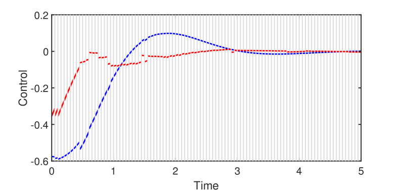
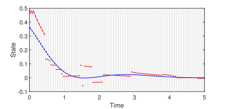
Figure 1: Switching controller and the resulting switching state trajectory (blue) and the corresponding parts of target demonstrations (red) with time intervals between switches (gray). The simulation of the quadcopter example (see description in Section 6.1., only one state and one control input) with the LQR switching controller produced by our implementation of Algorithm 2.

Now observe that unlike an individual tracking, such switching control laws are not unique due to the non-unique switching times. However, we can narrow our interest to switching controllers that have predefined switching times given as described in Section 5.1.

Now we will work with a differentiable Lyapunov-like functions $L\colon\mathbb{R}^{n}\mapsto\mathbb{R}$ that will serve as a reachability certificate. The intuition is that this function will satisfy a Lyapunov-like condition on demonstrations, which will then allow us to check reachability of the constructed tracking controller relative to the behavior of the demonstration it follows between two switches.

The Lyapunov-like condition on demonstrations is the following [42]:

Definition 5.

A differentiable function $L:\mathbb{R}^{n}\rightarrow\mathbb{R}$ is compatible with a set of demonstrations $\mathcal{T}$ iff there is $\delta<0$ such that for all $(\tilde{x},\tilde{u})\in\mathcal{T}$ and all $t\in[0,T]$

$$\nabla L(\tilde{x}(t))^{T}F(\tilde{x}(t),\tilde{u}(t))\leq\delta.$$

We want to use the function $L$ to ensure reachability of the resulting switching control law. For this, we will use a criterion similar to a finite-time Lyapunov functions [2]. We choose constants $1>\gamma>0$, $t_{\mathrm{min}}>0$ and define a switching control with the reachability certificate $L$ in such a way that we switch demonstrations after the minimum time $t_{\mathrm{min}}$ elapsed and the following decrease condition is met.

Definition 6.

A switching control law $u_{\mathrm{switch}}^{\mathcal{T}}$ is sufficiently decreasing on $I$ wrt. a function $L:\mathbb{R}^{n}\rightarrow\mathbb{R}$ and a goal set $G$ iff for every $x_{0}\in I\setminus G$, a switching trajectory $x=\Sigma(x_{0},u_{\mathrm{switch}}^{\mathcal{T}})$ with corresponding switching times $t_{1},t_{2},\dots$ and target demonstrations $(\tilde{x}_{1},\tilde{u}_{1}),(\tilde{x}_{2},\tilde{u}_{2}),\dots$ meets for every $j\geq 0$

• either $x(t_{j+1})\in G$,

• or $x(t_{j+1})\in I$ and $L(x(t_{j+1}))-L(x(t_{j}))\leq\gamma[L(\tilde{x}_{j}(t_{j+1}-t_{j}))-L(\tilde{x}_{j}(0))]$.

Here $t_{0}=0$.

This definition tests the decrease conditions exactly between two subsequent switching times. It would actually be possible to test the decrease condition less often than switching, but we avoid this to keep this definition and the subsequent implementation simple. Testing the decrease condition more often than switching would introduce significantly more severe complications that would make it necessary to make the check dependent on not only the state itself, but also the target demonstration used to reach this state.

Since such a switching control law decreases $L$ at least by

$$\sup_{(\tilde{x},\tilde{u})\in\mathcal{T}}\gamma\left[L(\tilde{x}(t_{\mathrm{min}}))-L(\tilde{x}(0))\right]$$

over one trajectory switch, which is enforced to be lesser than zero, the system must visit $G$ after finitely many trajectory switches, otherwise we get a contradiction with the fact that $L$ must be bounded (from below) over the set $I\setminus G$. Hence we now have a suitable definition of the notion of reachability certificate.

Definition 7.

A differentiable function $L:\mathbb{R}^{n}\rightarrow\mathbb{R}$ is a reachability certificate for a switching control law $u_{\mathrm{switch}}^{\mathcal{T}}$ based on a set of demonstrations $\mathcal{T}$ and a goal set $G$ iff

• it is compatible with $\mathcal{T}$, and

• $u_{\mathrm{switch}}^{\mathcal{T}}$ is sufficiently decreasing on $I$ wrt. $L$ and $G$

Note that formal verification of this property would require solving the given ODE precisely. This is indeed possible [36], and the given definition simplifies the task due to its restriction to solutions between switches.

The defined certificate proves reachability due to the following proposition whose proof the reader will find in the appendix.

Proposition 1.

The existence of a reachability certificate for a switching control law ensures that every system trajectory of the resulting closed loop system visits the goal set after finitely many trajectory switches.

4.3 Controller Synthesis Algorithm

It is time to instantiate the general algorithm from Section 3 to the switching control law from Definition 4. The result is Algorithm 2. The algorithm concretizes the construction of a generic control law using a family of tracking controllers $u_{\mathrm{track}}$.

Algorithm 2 Controller and Compatible Certificate Synthesis

Input:

• a control system of the form stated in Section 2

• a compact initial set $I$

• a compact goal set $G$

Output:

• a control law that steers the system from $I$ into $G$ and optionally satisfies some additional performance requirements, and

• a reachability certificate $L$

1. Generate an initial set of demonstrations $\mathcal{T}$.

2. Choose an open bounded set $W\supset I\setminus G$ on which the demonstrator is defined and a sequence $M$ of states from $W$ whose set of elements is a dense subset of $W$.

3. Iterate:

   1. Learn a reachability certificate candidate $L_{p}$ by computing parameter values $p$ s.t. $L_{p}$ is compatible with every demonstration $(\tilde{x},\tilde{u})\in\mathcal{T}$.

   2. Let $x_{0}$ be the next sample from the sequence $M$. Let $(\tilde{x},\tilde{u})=\phi(\mathcal{T},x_{0})$, $x=\Sigma(x_{0},u_{\mathrm{track}}^{(\tilde{x},\tilde{u})})$. Check if there is a $t\in\left[t_{\mathrm{min}},T\right]$ s.t.

      • either $x(t)\in I$ and $L_{p}$ is compatible with $(\tilde{x},\tilde{u})$ and

        $$L_{p}(x(t))-L_{p}(x(0))\leq\gamma[L_{p}(\tilde{x}(t))-L_{p}(\tilde{x}(0)),$$

      • or $x(t)\in G$.

      If this condition does not hold, generate a new demonstration starting from $x_{0}$ and add it to $\mathcal{T}$.

4. return a switching control law based on $\mathcal{T}$ with a reachability certificate $L_{p}$

The algorithm depends on the following parameters:

• a demonstrator generating demonstrations on some open superset $W$ of $I\setminus G$

• a tracking method that assigns to every demonstration $(\tilde{x},\tilde{u})$ a tracking controller $u_{\mathrm{track}}^{(\tilde{x},\tilde{u})}$

• a system of parametrized reachability certificate candidates $L_{p}(x),p\in P$

• an assignment rule $\phi$

• real numbers $1>\gamma>0$ and $t_{\mathrm{min}}>0$

Let us explore the inner workings of Algorithm 2 more closely. Algorithm 2 tests whether the constructed switching control law is sufficiently decreasing which, due to Proposition 1, ensures reachability. A suitable reachability certificate candidate $L$ is chosen to be compatible with demonstrations $\mathcal{T}$ that are generated as the algorithm progresses. It is assumed that $L$ is taken from a parametrized set of candidates $\{L_{p}(x)\mid p\in P\}$. System simulations in Algorithm 2 and the sufficient decrease condition are illustrated in Figure 2.

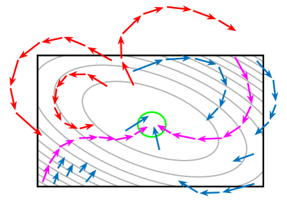
Figure 2: System simulations in Algorithm 2: goal set (green ellipse), demonstrations (magenta), reachability certificate candidate (contour plot) on the set of initial states $I$ (rectangle) compatible with these two demonstrations. Simulations that meet the sufficient decrease condition are blue, others are red.

The algorithm adds a new demonstration whenever it detects in the given time frame $[t_{\mathrm{min}},T]$ that the resulting switching controller does not meet Proposition 1, i.e. the corresponding tracking controller does not reach the goal set and the sufficient decrease condition is not met. If the tracking controller reaches the goal set or the sufficient decrease condition is met, the algorithm does not add a new demonstration. While the algorithm could decide whether to add a new demonstration purely by full simulations as in [44], thanks to the learned reachability certificate candidate $L$, states $x$ in at least some neighbourhoods of added demonstrations, as we describe later in Proposition 2, meet

$$L\left(\Sigma(x,u_{\mathrm{LQR}}^{\phi(\mathcal{T},x)})(t)\right)-L\left(\Sigma(x,u_{\mathrm{LQR}}^{\phi(\mathcal{T},x)})(0)\right)<\gamma\left[L(\tilde{x}(t))-L(\tilde{x}(0))\right]$$ (3)

for every $t\in\left[0,T\right]$. Hence, the algorithm detects the sufficient decrease condition for a such an $x$ the first time, when $\Sigma(x,u_{\mathrm{LQR}}^{\phi(\mathcal{T},x)})(t)\in I$ and $t\geq t_{\mathrm{min}}$.

In practice, this makes system simulations often significantly shorter (depending on lengths of demonstrations, times spent outside of $I$ and the quality of the reachability certificate candidate), and thus it makes the overall run of the algorithm noticeably faster, as we demonstrate in our numerical experiments.

Finally, notice that there is a slight discrepancy between Definition 6 and Algorithm 2, since the algorithm does test simulations from larger set $W\supset I\setminus G$, while the definition requires only simulations from $I\setminus G$ itself. This discrepancy is caused by the fact that algorithm checks the decrease condition via sampling and thus it requires an open investigated set. Otherwise, the algorithm could miss some states from which the decrease condition is not met, namely on the boundary of the investigated set. The expansion of the investigated set from $I$ to $W$ also implies that the demonstrator must provide demonstrations from $W$ as well.

4.4 Algorithm Properties

In this subsection, we will establish properties of Algorithm 2 in terms of reachability and asymptotic optimality of the resulting switching control law. First, we show that, in finitely many iterations, Algorithm 2 creates a feedback control law that reaches the goal set.

Let us begin with several assumptions. We start with the set of reachability certificate candidates.

1. We assume a set of parametrized reachability certificate candidates $\{L_{p}(x)\mid p\in P\},$ where the set of values of the parameters $P$ is compact. We further assume that $L_{p}(x)$ is continuous in both $p$ and $x$, and that for every $p\in P$, $L_{p}(x)$ is differentiable in $x$. Finally, we assume that the set of candidates includes a candidate that is compatible with all demonstrations generated by the demonstrator.

In addition, we add a technical, albeit crucial, assumption that ensures that the decrease condition is met while tracking any given demonstration closely enough.

1. We assume that there are is an $\varepsilon>0$ such that any demonstration $(\tilde{x},\tilde{u})$ includes a point $\tilde{x}(t)$ for some $t\geq t_{\mathrm{min}}$ such that an $\varepsilon$-neighbourhood with the center in $\tilde{x}(t)$ lies in either $I$ or $G$.

Further, we need to guarantee that the assignment rule $\phi$ always assigns sufficiently near demonstrations. This does not mean that the nearest demonstration has to be chosen. The chosen demonstration only has to approach the given point in the limit, as this point itself approaches an arbitrary demonstration (which may still be different from the chosen one).

Definition 8.

We will say that an assignment rule is dominated by the Euclidean norm iff for every $\alpha>0$ there is a $\beta>0$ such that for every finite set of demonstrations $\mathcal{T}$, for every $(\tilde{x},\tilde{u})\in\mathcal{T}$ and every $x_{0}\in\mathbb{R}^{n}$ such that $\left\lVert x_{0}-\tilde{x}(0)\right\rVert<\beta$, there exists a $(\tilde{x}^{\prime},\tilde{u}^{\prime})\in\mathcal{T}$ s.t. $\phi(\mathcal{T},x_{0})=(\tilde{x}^{\prime},\tilde{u}^{\prime})$, and $\left\lVert x_{0}-\tilde{x}^{\prime}(0)\right\rVert<\alpha$.

1. We assume that the assignment rule $\phi$ used in Algorithm 2 is dominated by the Euclidean norm.

Lastly, Algorithm 2 detects counterexamples—states that do not meet the decrease condition—via sampling using the sequence of states $M\subset W$ whose set of elements is a dense subset of $W$. Hence, we need to make certain that the presence of a counterexample implies the existence of a whole open ball of counterexamples in its vicinity. Otherwise the algorithm may not detect such a counterexample during the run of the algorithm at all. Keep in mind that due to continuity of ODEs solution wrt. initial conditions, there is a open ball of counterexamples around any given a counterexample provided that all states in this neighbourhood are assigned to the same demonstration. However, this cannot always be the case since any assignment rule is necessarily discontinuous for a finite set of demonstrations. Consequently, we need further restrict the assignment rule $\phi$ in case that a counterexample lies on a boundary between sets that are assigned to distinct demonstrations.

1. We assume that the assignment rule $\phi$ meets the following. For any finite set of demonstrations $\mathcal{T}$, and for any state $x\in\mathbb{R}^{n}$, and any $\varepsilon>0$, there is an open ball that is a subset of an $\varepsilon$-neighbourhood of $x$ and includes only states that are assigned via $\phi$ to the same trajectory as $x$.

Notice that an assignment rule based on the Euclidean distance meets Assumption ( IV ) since such an assignment rule partitions $\mathbb{R}^{n}$ into Voronoi polygons.

For our further discussion, we will reduce our attention to a single type of tracking, specifically a tracking controller based on the linear-quadratic regulator (LQR), for which we refer the reader to the literature [26, 22, 51, 44]. We will denote by $u_{\mathrm{LQR}}^{(\tilde{x},\tilde{u})}$ an LQR tracking controller of a demonstration $(\tilde{x},\tilde{u})$. This LQR controller is characterized by a solution of the differential Riccati equation. Further, we will assume that all cost matrices used in the construction of LQR tracking are positive definite and fixed for all demonstrations.

To derive the main result of this section, we first state a stronger continuity property for evolutions of the system with an LQR tracking controller wrt. their initial states. Namely, we show that for any given demonstration $(\tilde{x},\tilde{u})$, there is a neighbourhood around $\tilde{x}(0)$, independent of a particular choice of $(\tilde{x},\tilde{u})$, such that the evolutions of the system with an LQR tracking controller stays close to $(\tilde{x},\tilde{u})$. This holds due smoothness of $F$ and boundedness of all demonstrations to $X\times U$.

Hence, we can state the following lemma whose proof, which follows the structure of the proof of Lemma 4 in Tobenkin et. al. [52], the reader can find in the appendix.

Lemma 1.

For any $\varepsilon>0$ there is a $\delta>0$ such that for any $x_{0}\in\mathbb{R}^{n}$ and for any demonstration $(\tilde{x},\tilde{u})$ with $\left\lVert x_{0}-\tilde{x}(0)\right\rVert<\delta$ and for all $t\in[0,T]$,

$$\left\lVert\Sigma(x_{0},u_{\mathrm{LQR}}^{(\tilde{x},\tilde{u})})(t)-\tilde{x}(t)\right\rVert<\varepsilon.$$

Lemma 1 together with assumptions ( I )–( III ) assures that there is a neighbourhood around each initial point of any added demonstration, where the algorithm will not add any further demonstration. This is because all states in these neighbourhoods are assigned to close demonstrations due to ( III ), the corresponding LQR tracking controllers follows the assigned trajectory closely and eventually reaches the state where the decrease condition is met due to ( I ) and ( II ). Consequently, only finitely many demonstrations can be added during the whole run of the algorithm, because the investigated set $W$ is bounded. And after the last demonstration was added, no further counterexamples to the decrease condition can exist in $W$ because there would be a open ball of them due to ( IV ) and hence would be detected by the rest of the sequence $M$ whose set of elements is still a dense subset of $W$.

Notice additionally that Lemma 1 is the only piece that depends on our choice of tracking, namely it is stated for LQR tracking. Thus, the stated considerations and the following proposition holds under Assumptions ( I )–( IV ) for any type of tracking that meets its corresponding variant of Lemma 1.

Proposition 2.

Assume that Algorithm 2 uses the tracking controllers $u_{\mathrm{LQR}}$ and let Assumptions ( I )–( IV ) hold. Then, in finitely many iterations, Algorithm 2 provides a control law that steers the system from $W$ into $G$.

Moreover, after dropping Assumption ( I ) and with minor modifications of the proofs, this result also holds for the case without any use of certificates which corresponds to earlier methods [51, 44] that were published without such guarantees. For example, Reist et. al. [44] write “However, while the analysis shows that, in the long run, the algorithm tends to improve the generated policies, there are no guarantees for finite iterations.”

The LQR tracking controllers have another benefit in providing an assignment rule that respects the dynamics of the system where as the assignment rule based on the Euclidean distance does not. Namely, we set for a finite set of demonstrations $\mathcal{T}=\{(\tilde{x}_{1},\tilde{u}_{1}),\ldots,(\tilde{x}_{N},\tilde{u}_{N})\}$

$$\phi(x,\mathcal{T})=\underset{{i=1,\ldots,N}}{\mathrm{arg\,min}}\left\{(x-\tilde{x}_{i}(0))^{T}S_{i}(0)(x-\tilde{x}_{i}(0))\right\}$$ (4)

where $S_{i}$ is a solution to the appropriate differential Riccati equation used in the construction of LQR tracking and moreover, it equals the cost of tracking for the linearized dynamics. Note that rule $\eqref{LQRarule}$ is actually not a properly defined assignment rule, since it allows ties. These are situations in which a state $x$ could be assigned to multiple distinct demonstrations, since $\phi(x,\mathcal{T})\neq\{(\tilde{x}_{i},\tilde{u}_{i})\}$ for some $i\in\{1,2,\ldots,N\}$. These ties must be resolved by assigning each state to a single demonstration from $\phi(x,\mathcal{T})$. Notice, that the resolution of these ties is closely connected to assumption ( IV ).

Lemma 2.

Assignment rule (4) with any resolution of ties is dominated by the Euclidean norm, and meets assumption ( IV ) for some appropriate resolution of ties.

We can also establish asymptotic relative optimality of the switching control law as well, provided that the demonstrator is continuous and consistent.

Definition 9.

A demonstrator is

• continuous iff the provided control input $u$ is jointly continuous in both the initial state $x_{0}\in W$ and time $t\in[0,T]$, and

• consistent iff for all demonstrations $(x_{1},u_{1})$ and $(x_{2},u_{2})$ provided by the demonstrator and all $t_{1},t_{2}\in[0,T]$, if $x_{1}(t_{1})=x_{2}(t_{2})$, then $u_{1}(t_{1})=u_{2}(t_{2})$.

Continuity of the demonstrator assures that demonstrations that start from near states are similar. Consistency of the demonstrator results in unique cost associated with the demonstrator for each state of the system, regardless of past visited states. A consistent demonstrator also allows for more efficient generation of demonstrations, since each system trajectory with inputs $u$ generated by the demonstrator can be interpreted as an infinite number of demonstrations, each one starting from a different state of the generated trajectory. In addition, consistency allows us to use a switching controller without loosing relative optimality. Further note that a demonstrator that provides time dependent control inputs can still be consistent, if we consider time as another state of the system.

The following proposition, whose proof the reader can find in the appendix, extends the assumed continuity of the demonstrator to LQR tracking trajectories.

Lemma 3.

Assume a continuous demonstrator. Every LQR tracking trajectory

$$\Sigma(x_{0},u_{\mathrm{LQR}}^{(\tilde{x},\tilde{u})})\colon[0,T]\rightarrow\mathbb{R}^{n}$$

is, as a function of time, its initial state $x_{0}$ and the initial state $\tilde{x}(0)$ of its target demonstration $(\tilde{x},\tilde{u})$ continuous on some neighbourhood of $(\tilde{x}(0)$, $\tilde{x}(0))$.

Next, let us define for a system trajectory $(x,u)$ the accumulated cost (2) after time $t$ as

$$V_{t}(x,u):=\int_{0}^{t}P(x(\tau),u(\tau),\tau)\mathrm{d}\tau.$$ (5)

The cost of switching trajectory with tracking $u_{\mathrm{LQR}}^{(\tilde{x},\tilde{u})}$ converges to the cost of the target demonstration as their initial points converge (see the appendix for a proof).

Proposition 3.

Assume a finite set of demonstrations $\mathcal{T}$ provided by a continuous and consistent demonstrator and an assignment rule that is dominated by the Euclidean norm. Let $u_{\mathrm{switch}}^{\mathcal{T}}$ be a switching controller based on $u_{\mathrm{LQR}}$, and let $(\tilde{x},\tilde{u})$ be a continuous demonstration. Then for all $t\in[0,T]$,

$$\lim_{x_{0}\rightarrow\tilde{x}(0)}\left|\mathrm{cost}_{V_{t}}(x_{0},u_{\mathrm{switch}}^{\mathcal{T}})-\mathrm{cost}_{V_{t}}(\tilde{x}(0),\tilde{u})\right|=0.$$

The following corollary extends this performance guarantee to the whole set $W$.

Corollary 1.

Assume a continuous and consistent demonstrator and an assignment rule that is dominated by the Euclidean norm. Let $x_{0}^{1},x_{0}^{2},\dots$ be a sequence of states in $W$ whose set of elements is a dense subset of $W$. Let $(\tilde{x}_{1},\tilde{u}_{1})$, $(\tilde{x}_{2},\tilde{u}_{2})$, $\dots$ be the sequence of corresponding demonstrations generated by the demonstrator for $\tilde{x}_{1}(0)=x_{0}^{1},\tilde{x}_{2}(0)=x_{0}^{2},\dots$. For $k=1,2\dots$, let $\mathcal{T}_{k}=\{(\tilde{x}_{i},\tilde{u}_{i})\mid i\in\{1,\dots,k\}\}$, and let $u_{\mathrm{switch}}^{\mathcal{T}_{k}}$ be a corresponding switching control law for $u_{\mathrm{LQR}}^{(\tilde{x},\tilde{u})}$. Then

$$\lim_{k\rightarrow\infty}\left|\mathrm{cost}_{V_{t}}(x_{0},u_{\mathrm{switch}}^{\mathcal{T}_{k}})-\mathrm{cost}_{V_{t}}(x_{0},u)\right|\rightarrow 0$$

for all $x_{0}\in W$ and for all $t\in[0,T].$

In particular, the limit converges to an optimal controller, if the demonstrator provides optimal demonstrations. Consequently, if we sample the state space thoroughly enough, the cost of the control law will approach the cost of the demonstrator, and hence we can ensure the additional performance requirements by stating the termination condition of the algorithm via performance comparison with the demonstrator.

While the introduced properties of the algorithm ensure reachability in finitely many iterations, and relative optimality in the limit, they do not state an explicit criterion for terminating the loop. In industry, safety-critical systems are often verified by systematic testing. This can be reflected in the termination condition for the main loop by simply considering each loop iteration that does not produce a counter-example as a successful test. Based on this, in a similar way as related work [44], one could terminate the loop after the number of loop iterations that produced a successful test without any intermediate reappearance of a counterexample exceeds a certain threshold. One could also require certain coverage [13] of the set $I$ with successful tests. And for even stricter safety criteria, one can do formal verification of the resulting controller.

5 Implementation

In this section, we describe our implementation of Algorithm 2 which we will refer as LQR switching algorithm.

5.1 Time Discretization

Definition 5 (compatibility with demonstrations) and Algorithm 2 are formulated in continuous time. This makes the algorithm unsuitable for computer implementation. For discretizing time and at the same time preserving the properties of the algorithm, we use the following modification of Definition 5:

Definition 10.

Assume a set of demonstrations $\mathcal{T}$ and a sequence $\theta=(\theta_{1},\theta_{2},\ldots)$ such that $0\leq\theta_{1}<\theta_{2}<\cdots\leq T$. A function $L:\mathbb{R}^{n}\rightarrow\mathbb{R}$ is discretely compatible with $\mathcal{T}$ at time instants $\theta$ iff there is $\delta<0$ such that for all $(\tilde{x},\tilde{u})\in\mathcal{T}$ and for all $j=1,2,\ldots$

$$L(\tilde{x}(\theta_{j+1}))-L(\tilde{x}(\theta_{j}))\leq\delta.$$

Provided that we restrict the switching times in Definition 6 to time instants $\theta$, a discrete-time reachability certificate is all that is needed.

Corollary 2.

The existence of a discrete-time reachability certificate certificate at time instants $\theta$ for a switching control law ensures that every system trajectory of the resulting closed loop system visits $G$ after finitely many trajectory switches

This modification of the compatibility condition offers another advantage. Algorithm 2 makes the assumption, that the parametrized set of reachable certificate candidates $\{L_{p}(x)\mid p\in P\}$ includes a candidate that is compatible. Discrete-time compatibility gives the algorithm the needed flexibility to meet this assumption, since the choice of time instants allows the algorithm to enforce the compatibility conditions only on parts of demonstrations. The trade-off is that in the parts where compatibility is not enforced, the algorithm must continue with simulations. Thus, one extreme is compatibility according to Definition 5 (the certificate is used at any time), and another is full simulation (the certificate is never used). In practice, we use an algorithm between these two extremes that works as follows.

To extract as much information from the demonstrator as possible, we compute a demonstration consisting of $2N-1$ equidistant time steps $h$. These time steps are also used as our choice of the time instants $\theta$ for the purpose of discrete-time compatibility for each demonstration. From these original demonstrations, we generate $N$ demonstrations of length $N$, the $i$-th demonstration starting from the $i$-th step, $i\in\{0,\dots,N-1\}$. This means that with each added demonstration, actually multiple demonstrations are added into the set of current system of trajectories, ensuring consistency according to Definition 2. Here we even include demonstrations with initial points outside of $W$.

Notice that we learn $L$ only on $W$, i.e., for learning $L$, we only use states of demonstrations that lie in $W$. We estimate the rest—for the purpose of the evaluation of the decrease condition at time instants when the target demonstrations lie outside of $W$—using other learned values that lie on the corresponding original demonstration. More specifically, we estimate initial values using a value of some previous state of the original demonstration and we estimate final values using a value of some next state of the original demonstration. In this way, our estimate of the sufficient decrease is always larger than the actual value would be. An example of a run of our implementation is given in Figure 3.

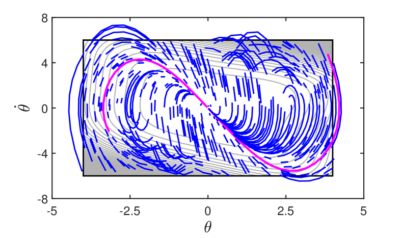
Figure 3: Several iterations of LQR switching algorithm for the pendulum example: demonstrations (magenta), reachability certificate candidate (contour plot) on the set of initial states $I$ (inner rectangle) compatible with these demonstrations, and system simulations in Algorithm 2 (blue). All system simulations are terminated, when the sufficient decrease condition is met.

5.2 Further Implementation Details

Our implementation uses LQR based tracking for following demonstrations using linearly interpolated numerical solutions of the appropriate differential Riccati equation. We choose the linear interpolation to make evaluation of control laws inexpensive. System solutions are numerically approximated using the RK4 integrator with a time step that is the same as the time step used in the computation of demonstrations.

We use assignment rule (4) with a slight modification: we first narrow the search of the target demonstration to the 100 closest demonstrations according to the Euclidean distance. This significantly speeds up the assignment for high dimensional examples with large number of generated demonstrations (namely, quadcopter example in our computational experiments).

We use a linearly parametrized set of certificate candidates: a set of polynomials. We choose the maximum degree for each problem in such a way that compatible reachability certificate candidate as described in Section 5.1 always existed during the computational experiments. Since candidates are parametrized linearly, we can learn reachability certificate candidates as solutions of the system of linear inequalities. In order to pick a reasonable candidate, we learn candidates as the Chebyshev center [42] of the polytope described by this system of linear inequalities. This selection strategy requires merely a solution of a linear program [9].

Lastly, we use use the following termination criterion for the main loop: Finish the loop, accepting the current strategy, if the number of simulations without finding a counter-example exceeds a certain threshold $N_{\mathrm{sim}}$.

5.3 Technical Solution

The whole implementation was done in MATLAB 2020b. The demonstrator is based on a direct optimal control solver [8] that solves the nonlinear programming problem which is obtained from the optimal control problem by discretization of the system dynamics and the cost [8]. The demonstrator was constructed using the toolbox CasADi v3.5.5 [4] with the internal optimization solver Ipopt [54]. Discretization was done via the Hermite-Simpson collocation method [18]. The initial solutions for the demonstrator were set as constant zero for both states and control with the exception of initial states. Apart from this, we used all solvers with their respective default settings.

6 Computational Experiments

Ex.	$T$	$h$	deg	$N_{\mathrm{sim}}$	$Q,R$
Pnd.	10	0.05	4	$2\cdot 10^{5}$	$I_{2},I_{1}$
Pndc.	10	0.05	2	$4\cdot 10^{5}$	$I_{4},I_{1}$
RTAC	150	0.05	4	$4\cdot 10^{5}$	$I_{4},I_{1}$
Acr.	10	0.01	4	$4\cdot 10^{5}$	$100I_{4},I_{1}$
Fan	40	0.05	2	$6\cdot 10^{5}$	$I_{6},I_{2}$
Quad.	20	0.05	2	$12\cdot 10^{5}$	$I_{12},I_{4}$

Table 1: Parameters of demonstrations and the LQR switching algorithm: length of demonstrations $T$, time step $h$, degree of the polynomial used for reachability certificate candidates, number of successful subsequent simulations to accept $N_{\mathrm{sim}}$, LQR cost matrices $Q$ and $R$

Ex.	$N_{\mathrm{dem}}$	$l_{\mathrm{sim}}$	$t_{\mathrm{sim}}$	$t_{\mathrm{total}}$	$N_{\mathrm{dem}}$	$l_{\mathrm{sim}}$	$t_{\mathrm{sim}}$	$t_{\mathrm{total}}$	$N_{\mathrm{dem}}$	$l_{\mathrm{sim}}$	$t_{\mathrm{sim}}$	$t_{\mathrm{total}}$
Pnd.	2	0.15	0.07	0.17	3	1.91	0.53	0.63	2	1.91	0.57	0.67
Pndc.	14	1.65	2.79	3.50	14	5.36	8.13	8.83	6	5.34	7.12	7.54
RTAC	4	2.75	5.04	10.92	11	73.18	213.87	227.60	TO	TO	TO	TO
Acr.	3	1.85	5.80	7.04	3	3.88	11.64	12.85	1	3.90	14.50	15.12
Fan	22	1.80	3.84	8.57	24	24.15	43.52	48.23	21	24.31	304.04	309.93
Quad.	98	1.64	28.01	1.64	111	7.53	154.81	178.63	∗73	∗7.53	∗562.69	∗590.25

Table 2: LQR switching algorithm (left), and simulation-only algorithm [44] with assignment rule (4) (middle) and assignment rule (6) (right): number of demonstrations added $N_{\mathrm{dem}}$, average lengths of simulations $l_{\mathrm{sim}}$, CPU time in minutes for simulations $t_{\mathrm{sim}}$, total CPU time in minutes $t_{\mathrm{total}}$. A star denotes that some runs exceed 10 hours CPU time mark (TO). All values are averages using 5 runs of the algorithms with different seeds of state samples.

Ex.	Dem	LQRsw	LQRtr	LQReq
Pnd.	$22$	$24$	$24$	$43$
Pndc.	$92$	$98$	$98$	$98$
RTAC	$297$	$401$	$430$	$636$ *
Acr.	$2516$	$7656$	$7669$	$8719$
Fan	$32$	$37$	$37$	$72$ *
Quad.	$45$	$50$	$50$	$69$

Table 3: Mean cost on 1000 random samples: demonstrator, LQR switching controller (the result of Algorithm 2), LQR tracking controller (the result of the simulation-only algorithm [44]), LQR controller around equilibrium. A star denotes that the controller failed from some samples, which were discarded from the mean value. All values for LQR switching controller and LQR tracking controller are averages using 5 runs of the algorithms with different seeds of state samples.

In this section, we provide computational experiments documenting the behavior of our algorithm and implementation on six typical benchmark problems. The problems range from dimension two to twelve and will concern the task of reaching a neighbourhood of an equilibrium. The cost functional is quadratic $V_{t}(x,u)=\int_{0}^{t}x(\tau)^{T}x(\tau)+u(\tau)^{T}u(\tau)\,\mathrm{d}\tau$.

We compare our LQR switching algorithm with the most similar algorithm from the literature: simulation based LQR trees [44]. This algorithm also employs demonstrations and LQR tracking, but neither uses a reachability certificate nor switching. Thus, it searches for counter-examples to reachability using full system simulations.

Another slight difference is in the choice of the assignment rule (4) which subsequently leads to an alteration in the strategy of adding new demonstrations. Let us denote $V_{i}(x)=(x-\tilde{x}_{i}(0))^{T}S_{i}(0)(x-\tilde{x}_{i}(0))$. Then the assignment rule in [44] is

$$\phi(x,\mathcal{T})=\underset{{i=1,\ldots,N}}{\mathrm{arg\,min}}\left\{V_{i}(x)\text{ s.t. }V_{i}(x)\leq d_{i}\right\},$$ (6)

where the values $d_{i}$ are learned during the run of the algorithm: when the algorithm detects a counterexample via a full system simulation, instead of adding a new demonstration immediately, the algorithm lowers the value of the corresponding $d_{i}$ such that the counterexample state is no longer assigned to the demonstration which led to failed reachability. Then the algorithm tries to assign a new demonstration via (6) with the modified values of $d_{i}$s. The algorithm adds a new demonstration only when no current demonstration can be assigned to the sampled point via assignment rule (6).

These modifications are still within the theory presented here and hence, the algorithm [44] still meets Proposition 2 and Corollary 1, i.e. constructs a control law that achieves reachability in finitely many iterations and that is asymptotically relatively optimal for increasing number of demonstrations.

For the sake of completeness, we will do our comparison between our algorithm and the full simulation algorithm [44] in two versions, with assignment rule (6) and with assignment rule (4) (both with a speed up using the Euclidean distance described in subsection 5.2). We are mostly interested in the effect of reachability certificate $L$ that should significantly speed up the simulation process, due to the sufficient decrease criterion from Definition 6.

Lastly, to make these examples (except the acrobot example) a bit more challenging , we also required the synthesized controller to stay within a prespecified simulation region $S\supset I$. We also added this condition as a constraint on demonstrations to the demonstrator.

6.1 Examples

Inverted pendulum

We use the model

$$\ddot{\theta}=\frac{g}{l}\sin\theta-\frac{b\dot{\theta}}{ml^{2}}+\frac{u}{ml^{2}},$$ (7)

where $x=\left[\theta,\dot{\theta}\right]$ and $m=1,l=0.5,g=9.81,b=0.1$. We set the initial set $I=\left[-4,4\right]\times\left[-6,6\right]$ extended to $W=\left(-4.05,4.05\right)\times\left(-6.05,6.05\right)$, and set the goal set $G=\{x\in\mathbb{R}^{2}\mid\left\lVert x\right\rVert<0.05\}$. Additionally, we set $S=\left[-5,5\right]\times\left[-8,8\right]$ beyond which both learning algorithms denoted simulations as unsuccessful.

Inverted pendulum on a cart

We use the model

$$\ddot{x} =\frac{4u+4ml\dot{\theta}^{2}\sin\theta-3mg\sin\theta\cos\theta}{4(M+m)-3m\cos^{2}\theta}$$ (8)

$$\ddot{\theta} =\frac{(M+m)g\sin\theta-u\cos\theta-ml\dot{\theta}^{2}\sin\theta\cos\theta}{l(\frac{4}{3}(M+m)-m\cos^{2}\theta)},$$

where $x=\left[x,\theta,\dot{x},\dot{\theta}\right]$ and $m=0.21,M=0.815,g=9.81$ a $l=0.305$. We set the initial set $I=\left[-2.5,2.5\right]\times\left[-2,2\right]\times\left[-2.5,2.5\right]\times\left[-2.5,2.5\right]$ extended to $W=\left(-2.55,2.55\right)\times\left(-2.05,2.05\right)\times\left(-2.55,2.55\right)\times\left(-2.55,2.55\right)$, and set the goal set $G=\{x\in\mathbb{R}^{4}\mid\left\lVert x\right\rVert<0.1\}$. Additionally, we set $S=\left[-8,8\right]\times\left[-3,3\right]\times\left[-12,12\right]\times\left[-8,8\right]$.

RTAC (Rotational/translational actuator)

We use the model [10] of dimension $4$. We set the initial set $I=\left[-5,5\right]^{4}$ extended to $W=\left(-5.1,5.1\right)^{4}$, and set the goal set $G=\{x\in\mathbb{R}^{4}\mid\left\lVert x\right\rVert<0.05\}$. Additionally, we set $S=\left[-8.5,8.5\right]^{4}$.

Inverted double pendulum (acrobot)

We use the same model as in [35] of dimension $4$. We set the initial set $I=\left[-0.17,17\right]^{4}$ extended to $W=\left(-0.175,175\right)^{4}$, and set the goal set $G=\{x\in\mathbb{R}^{4}\mid\left\lVert x\right\rVert<0.0001\}$. In this particular example, we did not specify the set $S$.

Caltech ducted fan

We use the planar model of a fan in hover mode [21] of dimension $6$. We set the initial set $I=\left[-1,1\right]^{6}$ extended to $W=\left(-1.05,1.05\right)^{6}$, and set the goal set $G=\{x\in\mathbb{R}^{6}\mid\left\lVert x\right\rVert<0.01\}$. Additionally, we set $S=\left[-5,5\right]^{6}$.

Quadcopter

We use the simplified quadcopter model from [16, (2.61)–(2.66)], where we set $m=1$ and $g=9.8$. We set the initial set $I=\left[-1,1\right]^{12}$ extended to $W=\left(-1.05,1.05\right)^{12}$ and set the goal set $G=\{x\in\mathbb{R}^{12}\mid\left\lVert x\right\rVert<0.01\}$. Additionally, we set $S=\left[-6,6\right]^{12}$.

6.2 Results

The problem-dependent parameters that we used are listed in Table 1. In addition, we used the time step for generation of demonstrations $h$ as the minimum switching time $t_{\mathrm{min}}$. We ran all algorithms for each example five times using five fixed sequences of samples $M$ generated via realization of the uniform distribution on the corresponding set $W$.

The comparison of our algorithm based on LQR switching, and the full simulation based algorithms can be found in Table 2. We also provide the resulting switching state trajectories for the pendulum example in Figure 4.

In the case of these benchmarks, the usage of assignment rule (6) leads to a smaller number of added demonstrations in comparison to assignment rule (4). The overall number of system simulations however increases due to a larger number of detected counterexamples overall (except pendulum on a cart example where assignment rule (6) is faster) so much so that we encountered a runtime larger than 10 hours for RTAC and quadcopter examples, which we declared as time outs. Hence, it seems that is overall a better strategy to simply keep adding new demonstrations whenever a counterexample to reachability is detected rather then modify the assignment rule in order to assign a different existing demonstration, which is what [44] does. We can also notice that average length of simulations $l_{\mathrm{sim}}$ is nearly identical for both, which is not surprising since both variants requires full system simulation to prove reachability.

If we compare Algorithm 2 to both full simulation algorithms, our algorithm provides noticeable time savings in system simulations (between 50% and 95%). This is because Algorithm 2 can declare a system simulation successful as soon as $t_{\mathrm{min}}$ passes provided that the decrease condition is met. Since the majority of the full simulation runs consists of system simulations (other two major parts are computing demonstrations and assignment of these demonstrations to samples), we can notice a significant time-savings in the overall runs of the algorithm as well.

We also evaluated the cost of the resulting controllers for 1000 random samples, see Table 3. For comparison, we also include the cost of the demonstrator and the cost of an LQR controller computed around the equilibrium (with cost matrices from Table 1). If we compare the mean cost in Table 3, the cost of LQR switching control and the cost of the LQR tracking controller are quite similar which illustrates that trajectory switching did not compromise the overall performance of the constructed controller. Hence, Algorithm 2 provides a control law of similar performance to the full simulation algorithms but significantly faster. Notice also that the LQR control law around the equilibrium has a higher mean value cost in comparison to the both tracking based LQR controllers, which shows that using demonstrations significantly decreased the cost.

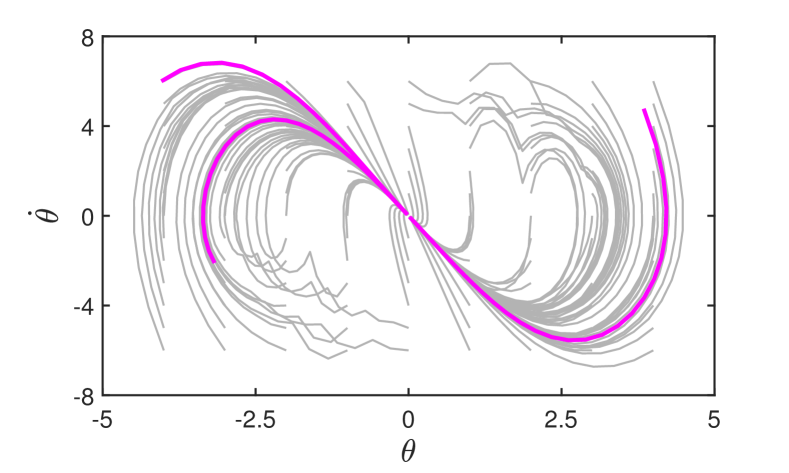
Figure 4: Solution produced by LQR switching algorithm: demonstrations (magenta) and switching state trajectories (gray).

7 Conclusion

We have proposed a framework for learning reachability Lyapunov-like certificates and synthesizing control laws that inherits optimality with respect to a chosen cost functional from the given demonstrator. We have stated a specific LQR variant of the given framework and provided some asymptotic guarantees. We have also implemented the algorithm and tested it on various case studies. We have made a time comparison with a full simulation approach and have seen significant time savings in learning reachability certificates.

Appendix A LQR tracking

First, we give a brief overview of LQR tracking with some observations, which we use throughout the proofs later. Let us denote $\Delta x(t)=x(t)-\tilde{x}(t)$ and $\Delta u(t)=u(t)-\tilde{u}(t)$. We set the cost of LQR tracking as

$$\int_{0}^{T}\Delta x(t)^{T}Q\Delta x(t)+\Delta u(t)^{T}R\Delta u(t)\;\mathrm{d}t\;+\Delta x(T)^{T}Q_{0}\Delta x(T)$$ (9)

for any demonstration $(\tilde{x},\tilde{u})$, where $Q,R$ and $Q_{0}$ are all positive definite matrices. and assume a linear system

$$\Delta\dot{x}(t)=A(t)\Delta x(t)+B(t)\Delta u(t),$$ (10)

where $A(t)=A(\tilde{x}(t),\tilde{u}(t))$ and $B(t)=B(\tilde{x}(t),\tilde{u}(t))$ is the linearization of the system dynamics $F$ around the demonstration $(\tilde{x},\tilde{u})$. Then, the LQR tracking controller is

$$u_{\mathrm{LQR}}^{(\tilde{x},\tilde{u})}(x,t)=-K(t)(x-\tilde{x}(t))+\tilde{u}(t),$$ (11)

where $K(t)=R^{-1}B(t)^{T}S(t)$. The matrix $S(t)$ meets the differential Riccati equation

$$-\dot{S}=Q+SA(t)+A(t)^{T}S-SB(t)R^{-1}B(t)^{T}S$$ (12)

with the terminal condition $S(T)=Q_{0}.$

Let us denote $V^{(\tilde{x},\tilde{u})}(x,t)=(x-\tilde{x}(t))^{T}S(t)(x-\tilde{x}(t))$. Note that $V^{(\tilde{x},\tilde{u})}(x,t)$ represents the optimal accumulated cost of tracking $u_{\mathrm{LQR}}^{(\tilde{x},\tilde{u})}$ for the linearized dynamics around $(\tilde{x},\tilde{u})$ from $x$ in time $t$ to $T$. This fact allows us to make the following observation which we use multiple times in our proofs.

• There are constants $c_{1},c_{2}>0$ such that for any LQR tracking $u_{\mathrm{LQR}}^{(\tilde{x},\tilde{u})}$ of any demonstration $(\tilde{x},\tilde{u})$,

  $$c_{1}I_{n}\leq S(t)\leq c_{2}I_{n}\text{ for all }t\in[0,T],$$ (13)

  where $I_{n}$ denotes the $n\times n$ identity matrix and the inequalities are understood in the sense of positive definiteness.

The inequality $S(t)\leq c_{2}I_{n}$ holds for some $c_{2}>0$, since the optimal cost $V^{(\tilde{x},\tilde{u})}(x,t)$ is bounded by the cost of evolutions of the linearized dynamics using zero tracking inputs. The cost of these evolutions is bounded, since they are fully determined by the values of Jacobian $A(\tilde{x}(t),\tilde{u}(t))$ which are bounded since $(\tilde{x},\tilde{u})$ are bounded by a bounded set $X\times U$ and $F$ is smooth. As for the second inequality, matrix $S(t)$ is positive definite for all $t<T$ for any demonstration $(\tilde{x},\tilde{u})$, since $S(T)=Q_{0}$ for any demonstration. Moreover, the eigenvalues of $S(t)$ cannot be arbitrarily small. This is because the rate of cost increase is bounded from below since both cost matrices $Q$ and $R$ are positive definite and both $A(\tilde{x}(t),\tilde{u}(t))$ and $B(\tilde{x}(t),\tilde{u}(t))$ are bounded. Thus differences $\Delta x(t)$ in a given eigenvector direction for the linearized dynamics cannot become arbitrarily small arbitrarily fast using arbitrarily small control inputs, i.e., produce overall arbitrarily small cost.

Lastly, we notice that for a linear system

$$\Delta\dot{x}=\left(A(t)-B(t)K(t)\right)\Delta x=\tilde{A}(t)\Delta x$$ (14)

using (12)

$$\dot{V}^{(\tilde{x},\tilde{u})}=2\Delta x^{T}S(A-BK)\Delta x+\Delta x^{T}\dot{S}\Delta x=-\Delta x^{T}\left(Q+K^{T}RK\right)\Delta x.$$ (15)

We will use this inferred equality in the proof of Proposition 2.

Appendix B Proof of Proposition 1

Proposition 1.

The existence of a reachability certificate for a switching control law ensures that every system trajectory of the resulting closed loop system visits the goal set after finitely many trajectory switches.

Proof.

Let $\mathcal{T}$ be a set of demonstrations that defines a switching control law $u_{\mathrm{switch}}^{\mathcal{T}}$ and let $L$ be a reachability certificate for $u_{\mathrm{switch}}^{\mathcal{T}}$. Assume a state $x_{0}\in I\setminus G$ and let $(x^{\mathcal{T}}_{\mathrm{switch}},u_{\mathrm{switch}}^{\mathcal{T}})$ be the corresponding switching trajectory from $x_{0}$, i.e., $x^{\mathcal{T}}_{\mathrm{switch}}(0)=x_{0}$. Let $(\tilde{x}_{0},\tilde{u}_{0})$ be the first assigned demonstration. According to Definition 6, there exists a time instant $t_{\mathrm{min}}\leq t_{0}\leq T$ and a state $x_{1}=x^{\mathcal{T}}_{\mathrm{switch}}(t_{0})$ in which the first trajectory switch happens. At this time instant, either $x_{1}\in G$ (we are done), or $x_{1}\in I$ and

$$L(x_{1})-L(x_{0})\leq\gamma\left[L(\tilde{x}_{0}(t_{0}))-L(\tilde{x}_{0}(0))\right].$$

Assume the latter and assume that the next assigned target trajectory is $(\tilde{x}_{1},\tilde{u}_{1})$. We control the system according to this trajectory until we hit a time instant $t_{1}+t_{0}$ and a state $x_{2}$ and so on. As a whole, we get a sequence of visited states $(x_{i})_{i=0,1,2,\ldots}$, a sequence of time instants $(t_{i})_{i=0,1,2,\ldots}$, and a sequence of assigned demonstrations $(\tilde{x}_{i},\tilde{u}_{i})_{i=0,1,2,\ldots}$ such that for every $i\in\{0,1,2,\dots\}$,

$$L(x_{i+1})-L(x_{i})\leq\gamma\left[L(\tilde{x}_{i}(t_{i}))-L(\tilde{x}_{i}(0))\right].$$

Since $L(x)$ is compatible with $\mathcal{T}$, necessarily $L(\tilde{x}(t))-L(\tilde{x}(0))<0$ for any initial state $\tilde{x}(0)$ of any trajectory in $\mathcal{T}$ and any time $t\in[0,T]$. Moreover, we know that $L(\tilde{x}(t))$ decreases monotonically and hence $L(\tilde{x}(t))-L(\tilde{x}(0))\leq L(\tilde{x}(t_{\mathrm{min}}))-L(\tilde{x}(0))$ for any $t\in[t_{\mathrm{min}},T]$, where $t_{\mathrm{min}}>0$ is the minimum switching time used in the construction of $(x^{\mathcal{T}}_{\mathrm{switch}},u_{\mathrm{switch}}^{\mathcal{T}})$.

Now let

$$C=\sup_{(\tilde{x},\tilde{u})\in\mathcal{T}}L(\tilde{x}(t_{\mathrm{min}}))-L(\tilde{x}(0))\leq\delta t_{\mathrm{min}}<0,$$ (16)

in which we used the mean value theorem together with the fact that $L$ is compatible with $\mathcal{T}$, i.e. $\nabla{L}^{T}(\tilde{x})F(\tilde{x},\tilde{u})\leq\delta$ for any demonstration. Thus

$$L(x_{i+1})-L(x_{i})\leq\gamma\left[L(\tilde{x}_{i}(t_{i}))-L(\tilde{x}_{i}(0))\right]\leq\gamma C<0$$

for all $i=0,1,2,\ldots.$ In other words, the value of $L(x)$ decreases in every step of the sequence at least by $\gamma C$. Since $L(x)$ is continuous on $I$, it is bounded from below on $I\setminus G$, and thus, some state in the sequence must be in $G$ after finitely many switches. ∎

Appendix C Proof of Proposition 2

We first prove Lemma 1 that we use in the proof of Proposition 2.

Lemma 1.

For any $\varepsilon>0$ there is a $\delta>0$ such that for any $x_{0}\in\mathbb{R}^{n}$ and for any demonstration $(\tilde{x},\tilde{u})$ with $\left\lVert x_{0}-\tilde{x}(0)\right\rVert<\delta$ and for all $t\in[0,T]$,

$$\left\lVert\Sigma(x_{0},u_{\mathrm{LQR}}^{(\tilde{x},\tilde{u})})(t)-\tilde{x}(t)\right\rVert<\varepsilon.$$

Proof.

We split the proof into two parts. In the first part, we will note some well known properties of funnels—sets that enclose all evolutions of the system within the sets themselves [52]. The second part covers the actual proof itself that follows the proof of Lemma 4 of Tobenkin et. al. [52].

1

In this part, we will briefly introduce the notion of a funnel around the demonstration $(\tilde{x},\tilde{u})$ that we will use in the proof. Assume a positive definite differentiable function $P(x,t)$ and differentiable function $\rho(t)$. A time-varying set of states $\mathcal{F}(t)=\{x\in\mathbb{R}^{n}\mid P(x-\tilde{x}(t),t)\leq\rho(t)\}$ is a funnel provided that

$$\dot{P}(x-\tilde{x}(t),t)<\dot{\rho}(t)$$ (17)

on the set $\{x\in\mathbb{R}^{n}\mid P(x-\tilde{x}(t),t)=\rho(t)\}$ for all $t\in[0,T]$. Due to (17), any evolution that starts in the funnel $\mathcal{F}$ stays inside the funnel.

To prove the lemma, we will construct a certain funnel around the demonstration $(\tilde{x},\tilde{u})$. Let $S(t)$ be the solution of Riccati equation (12) and set $P(x,t)=x^{T}S(t)x$.

We denote $V^{(\tilde{x},\tilde{u})}(x,t)=(x-\tilde{x}(t))^{T}S(t)(x-\tilde{x}(t))$. First, for a given $\varepsilon>0$, we pick a constant $\rho>0$ such that $\{x\in\mathbb{R}^{n}\mid V^{(\tilde{x},\tilde{u})}(x,t)\leq\rho\}\subset\{x\in\mathbb{R}^{n}\mid(x-\tilde{x}(t))^{T}(x-\tilde{x}(t))<\varepsilon\}$ for all $t\in[0,T]$. Such a $\rho>0$ necessarily exists due to (13). Such a set lies in the $\varepsilon$-neighbourhoods of the demonstration $(\tilde{x},\tilde{u})$, however this set is not generally a funnel and thus evolutions from within could leave. Hence, we will consider the rescaling [52]

$$V^{(\tilde{x},\tilde{u})}_{k}(x,t)=e^{k\frac{T-t}{T}}(x-\tilde{x}(t))^{T}S(t)(x-\tilde{x}(t))$$ (18)

parametrized by $k>0$, and corresponding funnel candidates

$$\mathcal{F}(t)=\{x\in\mathbb{R}^{n}\mid V^{(\tilde{x},\tilde{u})}_{k}(x,t)\leq\rho\}.$$ (19)

By increasing the value of $k,$ we reduce the size of the set $\mathcal{F}(t)$ when going backwards in time. We will show in the last part that there is indeed a value of $k$ that makes $\mathcal{F}(t)$ a funnel, i.e. condition (17) will be met. Then, any neighbourhood of $\tilde{x}(0)$ that lies within the funnel $\mathcal{F}(0)$ — which must exist due to (13) — meets the proposition we want to prove, since the funnel encloses all evolutions of the system within the funnel and and the funnel itself lies in the $\varepsilon$-neighbourhood of the demonstration for all $t$ due to our choice of $\rho$.

2

Consider the system $\dot{x}=F(x,u_{\mathrm{LQR}}^{(\tilde{x},\tilde{u})})$ that uses the LQR tracking controller. We compute the Taylor expansion with center $\tilde{x}$ of the right hand side of this differential equation. Then

$$\dot{x}(t)=F(\tilde{x}(t),\tilde{u}(t))+\left(\frac{\partial F}{\partial x}(\tilde{x}(t),\tilde{u}(t))-\frac{\partial F}{\partial u}(\tilde{x}(t),\tilde{u}(t))K(t)\right)\Delta x(t)+f(x(t),\tilde{x}(t),\tilde{u}(t),K(t),t),$$ (20)

where $f=(f_{1},\ldots f_{n})$ is the remainder in the Taylor formula with elements

$$f_{i}(x(t),\tilde{x}(t),\tilde{u}(t),K(t),t)=\Delta x(t)^{T}\nabla^{2}F_{i}(y(t),u_{\mathrm{LQR}}^{(\tilde{x},\tilde{u})})\Delta x(t),$$ (21)

where $y(t)=\tilde{x}(t)+c(t)\Delta x(t)$ for some $c(t)\in[0,1]$.

Let us denote $\tilde{A}(t)=A(t)-B(t)K(t)$, where $A(t)=\frac{\partial F}{\partial x}(\tilde{x}(t),\tilde{u}(t))$ and $B(t)=\frac{\partial F}{\partial u}(\tilde{x}(t),\tilde{u}(t))$. Hence, we get

$$\Delta\dot{x}(t)=\tilde{A}(t)\Delta x(t)+f(x(t),\tilde{x}(t),\tilde{u}(t),K(t),t).$$ (22)

Since $F$ is assumed to be smooth, and $(\tilde{x},\tilde{u})$ is bounded by $X\times U$, and $K(t)=-R^{-1}B(t)^{T}S(t)$ is bounded due to these observations and (13), there is an $\alpha>0$ such that for sufficiently small $\Delta x$,

$$|f_{i}|\leq\alpha\left\lVert\Delta x\right\rVert^{2}$$ (23)

for all $i=1,\ldots,n$.

Thus, if we compute the derivative of $V_{k}$ (18) along the dynamics $F(x,u_{\mathrm{LQR}}^{(\tilde{x},\tilde{u})})$ using expansion (22) and already inferred equality (15), we get

$$\dot{V}^{(\tilde{x},\tilde{u})}_{k}(\Delta x,t)=e^{k\frac{T-t}{T}}\left(2\Delta x^{T}Sf\right.-\left.\Delta x^{T}\left(Q+K^{T}RK+kS\right)\Delta x\right).$$ (24)

Now, notice that the derivative of $V^{(\tilde{x},\tilde{u})}_{k}$ is negative for all $t\in[0,T]$ and for sufficiently small $\left\lVert\Delta x\right\rVert$ provided that $k$ is large enough. The reason is that

$$\left|2\Delta x^{T}Sf\right|<\Delta x^{T}(Q+K^{T}RK+kS)\Delta x$$ (25)

for sufficiently small $\Delta x$ and $k$ large enough due to (23) and the fact that $S\geq c_{1}I$ due to (13).

Hence, $\mathcal{F}$ is a valid funnel. Additionally, any state that meets the inequality

$$\rho\geq\left|V^{(\tilde{x},\tilde{u})}_{k}(x,t)\right|\geq c_{1}e^{k}\left\lVert x-\tilde{x}(t)\right\rVert^{2}.$$ (26)

for a given $t\in[0,T]$ belongs to $\mathcal{F}(t)$. Consequently, all states that meet $\left\lVert x-\tilde{x}(t)\right\rVert^{2}\leq\frac{\rho}{c_{1}e^{k}}$ stay in the funnel $\mathcal{F}(t)$, and thus any state for which $\left\lVert x-\tilde{x}(0)\right\rVert<\sqrt{\frac{\rho}{c_{1}e^{k}}}$ meets $\left\lVert\Sigma(x,u_{\mathrm{LQR}}^{(\tilde{x},\tilde{u})})(t)-\tilde{x}(t)\right\rVert<\varepsilon$ for all $t\in[0,T]$ due to our choice of $\rho$, which is what we have wanted to prove.

All that remains to show is the fact that this found neighbourhood with $\delta=\sqrt{\frac{\rho}{c_{1}e^{k}}}$ is valid for any demonstration. Notice however that all the constants $\alpha,k$ and $\rho$ used in the construction of $\delta$ are chosen using upper estimates of $\left\lVert f\right\rVert$ and $V^{(\tilde{x},\tilde{u})}(x,t)$ over all possible demonstrations, and thus they are chosen independently of a particular demonstration $(\tilde{x},\tilde{u})$. This observation completes the proof. ∎

Proposition 2.

Assume that Algorithm 2 uses the tracking controllers $u_{\mathrm{LQR}}$ and let Assumptions ( I )–( IV ) hold. Then, in finitely many iterations, Algorithm 2 provides a control law that steers the system from $W$ into $G$.

Proof.

We split the proof into three parts. In the first part, we provide the overall proof of Proposition 2 itself. In parts two and three, we prove two auxiliary observations used in the first part.

1

The proof of this proposition is based on the following fact. Due to Assumptions ( I )–( III ), there is $\delta>0$ such that for any $x\in W$, any finite set of demonstrations $\mathcal{T}$ and any reachability certificate candidate $L_{p}$ compatible with $\mathcal{T}$, all states from the $\delta$-neighbourhood of $x$ meet decrease condition (6) provided that $\mathcal{T}$ contains a demonstration $(\tilde{x},\tilde{u})$ with $\tilde{x}(0)=x.$ Let us for now assume that this $\delta>0$ indeed exists. We will provide the proof of this fact in the second part.

Now, assume a run of Algorithm 2. As the algorithm progresses, it adds demonstrations whenever the decrease condition is not met. However, there is a $\delta$-neighbourhood around each initial point of any added demonstration, where the algorithm adds no further demonstration, since the decrease condition is met on this neighbourhood. Consequently, only finitely many demonstrations can be added during the whole algorithm, because the investigated set $W$ is bounded.

Let us consider the iteration, when the last demonstration is added. We will now try arrive at a contradiction from the assumption that there are still counterexamples to the decrease condition on $W$. Provided that the assignment rule meets Assumption ( IV ), the existence of any counterexample to decrease condition (6) implies the existence of a whole open ball of counterexamples as we will show in the third part of this proof.

However, this open ball of counterexamples will be detected during the remaining iterations of Algorithm 2, since the rest of the sequence still consists of a set of elements that is a dense subset of $W$ and hence, it includes a point in any open ball. Hence the algorithm must add further demonstrations during the rest of the run, which is a contradiction with our assumption that no further demonstrations will be added. This completes the proof, provided that the aforementioned bound $\delta$ and open balls of counterexamples indeed exist.

2

Here, we will show the existence of bound $\delta$ that we used in the first part. To do that, we combine several observations.

1. The parametrized set of candidates $\{L_{p}\mid p\in P\}$ meets Assumption ( I ). In particular, $L_{p}(x)$ is continuous in both $x$ and $p$ on a compact set $\bar{W}\times P$, where $\bar{W}$ denotes the closure of $W$. Hence, for any $\varepsilon_{1}>0$, there is $\delta_{1}>0$ such that for any $x,x^{\prime}\in W$ and $p\in P$, for which $\left\lVert x-x^{\prime}\right\rVert<\delta_{1}$, holds $\left|L_{p}(x)-L_{p}(x^{\prime})\right|<\varepsilon_{1}$. Thus, there is $\delta_{1}>0$ such that for any $p\in P$ and for all $\left\lVert x_{1}-x_{1}^{\prime}\right\rVert<\delta_{1}$ and $\left\lVert x_{2}-x_{2}^{\prime}\right\rVert<\delta_{1}$ holds

   $$L_{p}(x_{1})-L_{p}(x_{2})\geq L_{p}(x_{1}^{\prime})-L_{p}(x_{2}^{\prime})-2\varepsilon_{1}$$ (27)

   Consequently, the decrease condition for a system trajectory with endpoints $x_{1},x_{2}$ wrt. a target demonstration with endpoints $x_{1}^{\prime},x_{2}^{\prime}$ which is compatible with $L_{p}$

   $$L_{p}(x_{1})-L_{p}(x_{2})\geq\gamma(L_{p}(x_{1}^{\prime})-L_{p}(x_{2}^{\prime}))$$ (28)

   is met provided that

   $$\varepsilon_{1}\leq\frac{1-\gamma}{2}K\leq\frac{1-\gamma}{2}(L_{p}(x_{1}^{\prime})-L_{p}(x_{2}^{\prime})),$$ (29)

   where a constant $K>0$ for the given minimum switching time $t_{\mathrm{min}}>0$ exists due to Definition 5. To conclude, we have found $\delta_{1}$-neighbourhood of endpoints of any demonstration, where decrease condition is met.

2. The assignment rule $\phi$ is dominated by the Euclidean norm as stated in Assumption ( III ). Hence, repeating the definition, for any $\varepsilon_{2}>0$, there is a $\delta_{2}>0$ such that for any initial point of some demonstration $x^{\prime}$ and any $x$ that meet $\left\lVert x-x^{\prime}\right\rVert<\delta_{2}$, the initial point $x^{\prime\prime}$ of the trajectory assigned to $x$ meets $\left\lVert x-x^{\prime\prime}\right\rVert<\varepsilon_{2}.$

3. Lemma 1 holds. Consequently, for any $\varepsilon_{3}>0$, there is a $\delta_{3}>0$ such that for all $x_{0}$, $\tilde{x}(0)$ for which $\left\lVert x_{0}-\tilde{x}(0)\right\rVert<\delta$ and for all $t\in[0,T]$,

   $$\left\lVert\Sigma(x_{0},u_{\mathrm{LQR}}^{(\tilde{x},\tilde{u})})(t)-\tilde{x}(t)\right\rVert<\varepsilon.$$

4. Assumption ( II ) holds, i.e., there is a $\delta_{4}>0$ such that any demonstration has a point $x(t)$ after $t\geq t_{\mathrm{min}}$ such that the whole $\delta_{4}$-neighbourhood of $x(t)$ lies in $I$ or $G$.

We just need to combine observations (O1)–(O4). Due to these observations, there is a $\delta$-neighbourhood of any initial state of any demonstration such that all states in this neighbourhood are assigned to close trajectories due to observation (O2). These states evolve close to their assigned trajectories due to observation (O3) and these evolutions reach $W$ or $G$ due to observation (O4). There, the decrease conditions are met due to observation (O1) and (O3). Or more specifically, we compute $\delta_{1}$ and set $\varepsilon=\mathrm{min}\{\delta_{1},\delta_{4}\}$. Next, we substitute $\varepsilon_{3}=\varepsilon$ to gain $\delta_{3}$. Finally we substitute $\varepsilon_{2}=\delta_{3}$ to gain $\delta_{2}$. The resulting value of $\delta$ is $\delta=\delta_{2}$. ∎

3

Lastly, we show that the existence of any counterexample to decrease condition (6) implies the existence of a whole open ball of counterexamples.

To see that, assume a counterexample simulation $x(t)$ that is assigned to a demonstration $(\tilde{x},\tilde{u})$. We first show that there is a time-varying neighbourhood $H(t)$ around $x(t)$ for all $t\in[t_{\mathrm{min}},T]$ such that all states in $H(t)$ could be a part of a counterexample simulation starting in $x(0)$ that is assigned to $(\tilde{x},\tilde{u})$. We will for now ignore the fact that any system trajectory must meet system ODE (1). Let us assume for a contradiction that there is no such a neighbourhood $H(t)$ for all $t$. We choose a sequence of positive numbers $\varepsilon_{1}>\varepsilon_{2}>\cdots$ and then pick of a corresponding sequence of states $x_{1},x_{2},\ldots$ on the trajectory $x(t)$ for $t\in[t_{\mathrm{min}},T]$ such that any $x_{i}$ has a $\varepsilon_{i}$-neighbourhood that includes a state that is not a possible part of a counterexample simulation, i.e. state $x^{\prime}$ such that $x^{\prime}$ lies in $G$, or $x^{\prime}$ lies in $I\setminus G$ and $L_{p}(x^{\prime})-L_{p}(x(0))\leq\gamma\left[L_{p}(\tilde{x})-L_{p}(\tilde{x}(0))\right]$.

The sequence $(x_{i})$ has a convergent subsequence $(x_{j})$ that converges to a state $x$ that lies on the trajectory $x(t)$ since the trajectory is compact. However, the state $x$ is a part of the counterexample simulation and thus, either $x$ lies in $\mathbb{R}^{n}\setminus(I\cup G)$, or $x$ lies in $I\setminus G$ and $L_{p}(x)-L_{p}(x(0))>\gamma\left[L_{p}(\tilde{x})-L_{p}(\tilde{x}(0))\right]$. If $x$ lies in $\mathbb{R}^{n}\setminus(I\cup G)$, then some whole neighbourhood $H$ of $x$ lies in $\mathbb{R}^{n}\setminus(I\cup G)$, since $I\cup G$ is compact. But $H$ also includes states of the subsequence $(x_{j})$ for large enough $j$ which also converges to $x$. That leads to a contradiction with the construction of $(x_{j})$. If $x$ lies in $I\setminus G$ and $L_{p}(x)-L_{p}(x(0))>\gamma\left[L_{p}(\tilde{x})-L_{p}(\tilde{x}(0))\right]$, then again, there is a whole neighbourhood $H$ of $x$ that lies in $I\setminus G$, because $G$ is compact, and $L_{p}(x^{\prime})-L_{p}(x(0))>\gamma\left[L_{p}(\tilde{x})-L_{p}(\tilde{x}(0))\right]$ for all $x^{\prime}\in H$, because $L$ is continuous. Hence, we obtain again a contradiction. To conclude, such a time-varying neighbourhood $H(t)$ around $x(t)$ must exist, which implies that all states in some neighbourhood $H^{\prime}(t)\subset H(t)$ of $x(t)$ could be a part of some counterexample simulation that starts sufficiently close to $x(0)$ due to continuity of $L$. Consequently, due to continuity of ODE solutions wrt. to initial conditions and Assumption ( IV ), there is a open ball in some neighbourhood of $x(0)$ from which all system simulations are counterexamples.

Appendix D Proof of Lemma 2

Lemma 2.

Assignment rule (4) with any resolution of ties is dominated by the Euclidean norm, and meets assumption ( IV ) for some appropriate resolution of ties.

Proof.

Let $\mathcal{T}=\{(\tilde{x}_{1},\tilde{u}_{1}),\ldots,(\tilde{x}_{N},\tilde{u}_{N})\}$ and let us denote $V_{i}(x)=(x-\tilde{x}_{i}(0))^{T}S_{i}(0)(x-\tilde{x}_{i}(0))$, where $S_{i}$ is a solution to the appropriate Riccati equation. We assume assignment rule (4)

$$\phi(x,\mathcal{T})=\underset{{i=1,\ldots,N}}{\mathrm{arg\,min}}V_{i}(x)$$ (30)

We first show that $\phi$ is dominated by the Euclidean norm.

Let us denote the demonstration assigned to a state $x$ by $\tilde{x}_{x}$. For a given $\alpha>0$, we need to find some $\beta>0$ such that for any $N>0$ and any $\mathcal{T}=\{(\tilde{x}_{1},\tilde{u}_{1}),\ldots,(\tilde{x}_{N},\tilde{u}_{N})\}$ and any $i=1,\ldots,N$ and any $x\in\mathbb{R}^{n}$, $\left\lVert x-\tilde{x}_{i}(0)\right\rVert<\beta$ implies $\left\lVert x-\tilde{x}_{x}(0)\right\rVert<\alpha$. We know due to (13) that

$$c_{1}\left\lVert x-\tilde{x}_{i}(0)\right\rVert^{2}\leq V_{i}(x)\leq c_{2}\left\lVert x-\tilde{x}_{i}(0)\right\rVert^{2}$$ (31)

for all $i=1,\ldots,N$. Hence, if $\left\lVert x-\tilde{x}_{i}(0)\right\rVert<\sqrt{\frac{c_{1}}{c_{2}}}\alpha=\beta$ for some $i$, necessarily

$$V_{x}(x)=(x-\tilde{x}_{x}(0))^{T}S_{x}(0)(x-\tilde{x}_{x}(0))\leq V_{i}(x)\leq c_{2}\left\lVert x-\tilde{x}_{i}(0)\right\rVert^{2}<c_{1}\alpha^{2},$$ (32)

and consequently,

$$c_{1}\alpha^{2}>V_{x}(x)\geq c_{1}\left\lVert x-\tilde{x}_{x}(0)\right\rVert^{2}$$ (33)

which is what we have wanted to show.

Next, we want show that $\phi$ meet Assumption ( IV ) with a proper resolution of ties. We first notice that Assumption ( IV ) necessarily holds for all $x$ in which $V_{i}(x)<V_{j}(x)$ for all $j\in\{1,\ldots,N\}$ such that $j\neq i$ due to continuity of all $V_{j}$s. Hence, we are only interested in ties, where $V_{i}(x)=V_{j}(x)$ for some distinct $i$ and $j$ and $V_{i}(x)\leq V_{k}(x)$ for all $k\in\{1,\ldots,N\}$.

Let us assume such a tie and without loss of generality, let us shift $x$ to the origin. The state $x$ meets (we will write further $\tilde{x}=\tilde{x}(0)$ and $S=S(0)$ for short)

$$\tilde{x}_{i_{1}}^{T}S_{i_{1}}\tilde{x}_{i_{1}}=\cdots=\tilde{x}_{i_{K}}^{T}S_{i_{K}}\tilde{x}_{i_{K}}$$ (34)

where the tie is in indices $K=\{i_{1},\ldots,i_{K}\}$. Now, we want to show that in any neighbourhood of $x$, there is an open ball only containing states that are all assigned to one index $k\in K$.

First, we find an index $k_{\mathrm{max}}\in K$ such that $\left\lVert\nabla V_{k_{\mathrm{max}}}(x)\right\rVert$ is maximal on $K$. If there is no other index in $K$ with the same norm of gradient at $x$, we are done, since there would be $y$ in the direction of $\nabla V_{k_{\mathrm{max}}}(x)$ from $x$ such that $V_{k_{\mathrm{max}}}(y)<V_{k}(y)$ for all $k\neq k_{\mathrm{max}}$. In addition, using the same reasoning, there must be other indices $l\neq k_{\mathrm{max}}\in K$ such that these gradients are equal to $\nabla V_{k_{\mathrm{max}}}(x)$, i.e.,

$$\nabla V_{k_{\mathrm{max}}}(x)=-2S_{k_{\mathrm{max}}}\tilde{x}_{k_{\mathrm{max}}}=-2S_{l}\tilde{x}_{l}=\nabla V_{l}(x)$$ (35)

otherwise, we would be done as well. Let us denote set of all such indices by $L$. Then there is $y$ in any given neighbourhood of $x$ in the direction of $\nabla V_{i_{\mathrm{max}}}(x)$ such that for all indices $k\in K$ is $V_{k}(y)<V_{j}(x)$ for all $j\in M\setminus K.$ Due to continuity, this inequality holds on a whole neighbourhood of $y$ which we denote $H$.

Now, let us assume that this neighbourhood does not contain an open ball of states that are assigned to the same demonstration. This is possible only when there is a tie for all $z\in H$. However, we can now split all states $z\in H$ into finitely many categories according to in which indices the tie is and which gradients are greatest in terms of the norm. Since the states $z$ covers the whole neighbourhood $H$ and the number of categories is finite, there must be a category that contains $n$ (the dimension of the state space) linearly independent states $w\in H$. Otherwise the states from all finitely many categories could not cover the whole $H$.

Hence, using the same argumentation as previously for $x$, there must be two indices $k_{1}$ and $k_{2}$ such that

$$S_{k_{1}}(w-\tilde{x}_{k_{1}})=S_{k_{2}}(w-\tilde{x}_{k_{2}}),$$ (36)

where $w$ are $n$ linearly independent vectors from the category corresponding to the tie $V_{k_{1}}(w)=V_{k_{2}}(w)$ with those two having the greatest norm of gradient. Since (36) must hold for $n$ linearly independent vectors, $S_{k_{1}}$ must equal $S_{k_{2}}$. Which in turn implies from (35) that $\tilde{x}_{k_{1}}=\tilde{x}_{k_{2}}$. Hence, there cannot be a tie for all $z\in H$ if the set of demonstrations is distinct, which completes the proof. ∎

Appendix E Proof of Proposition 3

We first prove Lemma 3 that we use in the proof of Proposition 3.

Lemma 3.

Assume a continuous demonstrator. Every LQR tracking trajectory

$$\Sigma(x_{0},u_{\mathrm{LQR}}^{(\tilde{x},\tilde{u})})\colon[0,T]\rightarrow\mathbb{R}^{n}$$

is, as a function of time, its initial state $x_{0}$ and the initial state $\tilde{x}(0)$ of its target demonstration $(\tilde{x},\tilde{u})$ continuous on some neighbourhood of $(\tilde{x}(0)$, $\tilde{x}(0))$.

Proof.

Let us denote the LQR tracking trajectory $\Sigma(x_{0},u_{\mathrm{LQR}}^{(\tilde{x},\tilde{u})})$ simply by $x$ and note that it is a function of time, its initial state and the initial state of its target trajectory. We first observe that $x$ is a solution of the ODE

$$\dot{x} =F(x,\tilde{u}(t,\tilde{x}(0))-K(t,\tilde{x}(0))\left[x-\tilde{x}(t,\tilde{x}(0)))\right])$$

$$x(0) =x_{0},$$ (37)

where the functions $\tilde{x}(t,\tilde{x}(0))$ and $\tilde{u}(t,\tilde{x}(0))$ denote the states and the controls of the target demonstration that is assigned to $x_{0}$, and where $K(t,\tilde{x}(0))$ is the solution of the Riccati equation that corresponds to the LQR tracking problem.

We will first show that $x$ depends on $x_{0}$ and $\tilde{x}(0)$ continuously. Let us interpret $\tilde{x}(0)$ as a specific value of a parameter $\lambda\in W$

$$\dot{x} =F(x,\tilde{u}(t,\lambda)-K(t,\lambda)\left[x-\tilde{x}(t,\lambda)\right])$$

$$x(0) =x_{0}$$ (38)

$$\lambda =\tilde{x}(0).$$

We know that $\tilde{u}(t,\lambda)$ and $\tilde{x}(t,\lambda)$ are jointly continuous in both $t$ and $\lambda$. Moreover,

$$K(t,\lambda)=-R^{-1}B(\tilde{x}(t,\lambda),\tilde{u}(t,\lambda))^{T}S(t,\lambda)$$

is obtained from a solution of the Riccati equation

$$-\dot{S}=Q-SB(\tilde{x}(t,\lambda),\tilde{u}(t,\lambda))R^{-1}B(\tilde{x}(t,\lambda),\tilde{u}(t,\lambda))^{T}S+SA(\tilde{x}(t,\lambda),\tilde{u}(t,\lambda))+A(\tilde{x}(t,\lambda),\tilde{u}(t,\lambda))^{T}S,$$ (39)

where $S(T)=Q_{0}$, $A(x,u)=\frac{\partial F(x,u)}{\partial x}$, $B(x,u)=\frac{\partial F(x,u)}{\partial u}$, and $Q,Q_{0}$ and $R$ are some positive definite matrices. A solution to the Riccati equation exists on $[0,T]$ due to [22, Theorem 6.4]. Moreover, since both $A$ and $B$ are smooth and both $\tilde{x}(t,\lambda),\tilde{u}(t,\lambda)$ are jointly continuous in $t$ and $\lambda$, the right hand side is locally Lipschitz in $S$ uniformly in $t$ and $\lambda$ due to [24, Lemma 3.2]. Thus, the solution $S(t,\lambda)$ is continuous in parameter $\lambda$ on $W$ uniformly for $t\in\left[0,T\right]$ due to [24, Theorem 3.5] and thus, $K(t,\lambda)$ is jointly continuous in $t$ and $\lambda$.

Consequently, the right hand side of (E) and its partial derivative wrt. $x$ are jointly continuous in $x$, $t$ and $\lambda$. Hence, the right hand side of (E) is also locally Lipschitz in $x$ uniformly for $t\in\left[0,T\right]$ and $\lambda\in W$ on any bounded subset of $\mathbb{R}^{n}$ due to [24, Lemma 3.2]. In addition, state trajectory $\tilde{x}$ as a solution to ODE (E) implies existence of solutions on some neighbourhood of $\tilde{x}(0)$ due to [20, Section 7.3]. These solutions $x$ are jointly continuous in both $x_{0}$ and $\lambda$ uniformly in $t\in\left[0,T\right]$ due to [24, Theorem 3.5]. This together with the continuity of $x$ in $t$, implies joint continuity of $x$ in all three arguments on such a neighbourhood. ∎

Proposition 3.

Assume a set of demonstrations $\mathcal{T}$ provided by a continuous and consistent demonstrator and an assignment rule that is dominated by the Euclidean norm. Let $u_{\mathrm{switch}}^{\mathcal{T}}$ be a switching controller based on $u_{\mathrm{LQR}}$, and let $(\tilde{x},\tilde{u})$ be a continuous demonstration. Then for all $t\in[0,T]$,

$$\lim_{x_{0}\rightarrow\tilde{x}(0)}\left|\mathrm{cost}_{V_{t}}(x_{0},u_{\mathrm{switch}}^{\mathcal{T}})-\mathrm{cost}_{V_{t}}(\tilde{x}(0),\tilde{u})\right|=0.$$

Proof.

First, we will show the proposition for a single LQR tracking trajectory, i.e., without switching. Let us assume two demonstrations $(\tilde{x},\tilde{u})$ and $(\tilde{x}^{\prime},\tilde{u}^{\prime})$, and let us denote $x=\Sigma(x_{0},u_{\mathrm{LQR}}^{(\tilde{x}^{\prime},\tilde{u}^{\prime})})$. We will show that the cost of trajectory $x$ tends to $(\tilde{x},\tilde{u})$ as $x_{0}$ tends to $\tilde{x}(0)$.

Notice first that $x$ and $(\tilde{x},\tilde{u})$ must stay close to each other. Since LQR tracking is of the form

$$u_{\mathrm{LQR}}^{(\tilde{x}^{\prime},\tilde{u}^{\prime})}(t)=\tilde{u}^{\prime}(t)-K(\tilde{x}^{\prime}(0),t)(x(t)-\tilde{x}^{\prime}(t)),$$

we see that, if $x_{0}=\tilde{x}^{\prime}(0)$, $x(t)=\tilde{x}^{\prime}(t)$ then $u_{\mathrm{LQR}}^{(\tilde{x}^{\prime},\tilde{u}^{\prime})}(t)=\tilde{u}^{\prime}(t)$ for all $t\in[0,T]$. Hence, using continuity of $x$ wrt. $x_{0}$, for any $\varepsilon^{\prime}>0$, there is a neighbourhood $H$ of $\tilde{x}^{\prime}(0)$ such that for any $x_{0}\in H$ and for all $t\in\left[0,T\right]$

$$\left\lVert(x(t),u_{\mathrm{LQR}}^{(\tilde{x}^{\prime},\tilde{u}^{\prime})}(t))-(\tilde{x}^{\prime}(t),\tilde{u}^{\prime}(t))\right\rVert<\varepsilon^{\prime}.$$

Additionally, due to continuity of the demonstrator, there is a neighbourhood $H^{\prime\prime}$ of $\tilde{x}(0)$ such that for all $\tilde{x}^{\prime}(0)$ in this neighbourhood

$$\left\lVert(\tilde{x}(t),\tilde{u}(t))-(\tilde{x}^{\prime}(t),\tilde{u}^{\prime}(t))\right\rVert<\varepsilon^{\prime\prime}.$$

Thus, there is a neighbourhood $H$ of $\tilde{x}(0)$ such that for all $x,\tilde{x}^{\prime}(0)\in H$

$$\left\lVert(x(t),u_{\mathrm{LQR}}^{(\tilde{x}^{\prime},\tilde{u}^{\prime})}(t))-(\tilde{x}(t),\tilde{u}(t))\right\rVert<\varepsilon.$$

Since $x$ and $(\tilde{x},\tilde{u})$ stay close to each other, their cost must be close as well. To show that we use the Taylor expansion of $P$ and get

$$\mathrm{cost}_{V_{t}}(x_{0},u_{\mathrm{LQR}}^{(\tilde{x}^{\prime},\tilde{u}^{\prime})})=\int_{0}^{t}P(\tilde{x}(\tau),\tilde{u}(\tau),\tau)\,\mathrm{d}\tau+\int_{0}^{t}r(x(\tau),u_{\mathrm{LQR}}^{(\tilde{x}^{\prime},\tilde{u}^{\prime})}(\tau),\tau)\,\mathrm{d}\tau,$$ (40)

where $r(x(\tau),u_{\mathrm{LQR}}^{(\tilde{x}^{\prime},\tilde{u}^{\prime})}(\tau),\tau)$ is the remainder in the Taylor formula which can be written in the Lagrange form as

$$r(x(\tau),u_{\mathrm{LQR}}^{(\tilde{x}^{\prime},\tilde{u}^{\prime})}(\tau),\tau)=(y-\tilde{y})^{T}\nabla P(y_{c},\tau),$$ (41)

where $y=(x,u_{\mathrm{LQR}}^{(\tilde{x}^{\prime},\tilde{u}^{\prime})})^{T}$ and $\tilde{y}=(\tilde{x},\tilde{u})^{T}$, and where $y_{c}=(\tilde{y}(\tau)+c(\tau)(y(\tau)-\tilde{y}(\tau))$ for some $c(\tau)\in\left[0,1\right]$. Since $P$ is smooth, and $\tilde{x},\tilde{x}^{\prime}$ and $\tilde{u},\tilde{u}^{\prime}$ are bounded to $X$ or $U$ respectively, we can estimate the remainder for sufficiently small differences $y-\tilde{y}$ as

$$\left\lVert r(x(\tau),u_{\mathrm{LQR}}^{(\tilde{x}^{\prime},\tilde{u}^{\prime})}(\tau),\tau)\right\rVert\leq C\varepsilon$$

for some $C>0$ and hence

$$\left|\mathrm{cost}_{V_{t}}(x_{0},u_{\mathrm{LQR}}^{(\tilde{x}^{\prime},\tilde{u}^{\prime})})-\mathrm{cost}_{V_{t}}(\tilde{x}(0),\tilde{u})\right|\leq Ct\varepsilon.$$

Thus, the cost of $x$ tends to the demonstrator’s cost as the initial points tends to each other.

We proved that individual LQR tracking trajectories stay close to the original demonstrations. But overall switching trajectory might not. Even if a switching trajectory starts from an initial point of some demonstration, the switching controller switches after a while to a new demonstration. This new demonstration could be completely different from the rest of the former demonstration that the controller originally followed. Thus, Proposition (3) would not hold. This where the continuity and consistency of the demonstrator comes in.

Assume a demonstration $(\tilde{x},\tilde{u})$ and a time instant $t_{1}\in[0,T]$. Due to consistency, a demonstration $(\tilde{x}_{1},\tilde{u}_{1})$ starting from $\tilde{x}_{1}(0)\equiv\tilde{x}(t_{1})$ meets

$$(\tilde{x}(t),\tilde{u}(t))=(\tilde{x}_{1}(t-t_{1}),\tilde{u}_{1}(t-t_{1}))$$

for all $t\in[t_{1},T],$ i.e. these corresponding segments of demonstrations are identical. Moreover, if we consider another demonstration $(\tilde{x}_{2},\tilde{u}_{2})$, then due to continuity of the demonstrator

$$\lim_{\tilde{x}_{2}(t_{1})\rightarrow\tilde{x}_{1}(0)}(\tilde{x}_{2}(t-t_{1}),\tilde{u}_{2}(t-t_{1}))=(\tilde{x}(t),\tilde{u}(t))$$

for all $t\in[t_{1},T],$ i.e., any segments with initial states close to each other stay also close.

With this observation in mind, we are ready prove the proposition itself. Let $0<t\leq T$ and consider a switching trajectory

$$(x^{\mathcal{T}}_{\mathrm{switch}},u_{\mathrm{switch}}^{\mathcal{T}})$$

with $N$ switches that ends with a state $x^{\mathcal{T}}_{\mathrm{switch}}(t)$ in an $\varepsilon_{1}$-neighbourhood of $\tilde{x}(t)$. Such a switching trajectory exists, since any switching trajectory starting from $\tilde{x}(0)$ is identical to the demonstration $(\tilde{x},\tilde{u})$ due to domination of the assignment rule by the Euclidean norm. Notice also that $N$ is necessarily bounded since there is a non-zero minimum time interval between the switches.

Let $t_{N}$ be the time instant of the last switch. Due to continuity of the tracking trajectory and domination of the assignment rule, there is an $\varepsilon_{2}>0$ such that all switching trajectories $(x^{\mathcal{T}}_{\mathrm{switch}},u_{\mathrm{switch}}^{\mathcal{T}})$ with a state in the $\varepsilon_{2}$-neighbourhood of $\tilde{x}(t_{N})$ in time $t_{N}$ meet

$$\left\lVert(x^{\mathcal{T}}_{\mathrm{switch}}(\tau),u_{\mathrm{switch}}^{\mathcal{T}}(\tau))-(\tilde{x}(\tau),\tilde{u}(\tau))\right\rVert<\varepsilon_{1}$$

for all $\tau\in\left[t_{N},t\right]$, regardless of the exact assigned demonstrations (remember that the demonstrator is continuous and consistent). We will repeat the argument for the second last switch $t_{N-1}$ and find an $\varepsilon_{3}>0$ such that all switching trajectories $(x^{\mathcal{T}}_{\mathrm{switch}},u_{\mathrm{switch}}^{\mathcal{T}})$ with a state in the $\varepsilon_{3}$-neighbourhood of $\tilde{x}(t_{N-1})$ in time $t_{N-1}$ meet

$$\left\lVert(x^{\mathcal{T}}_{\mathrm{switch}}(\tau),u_{\mathrm{switch}}^{\mathcal{T}}(\tau))-(\tilde{x}(\tau),\tilde{u}(\tau))\right\rVert<\varepsilon_{2}$$

for all $\tau\in\left[t_{N-1},t_{N}\right]$. We continue these steps. In the end, we will find an $\varepsilon_{N+1}$-neighbourhood of $\tilde{x}(0)$ such that all switching trajectories with an initial state in this neighbourhood

$$\left\lVert(x^{\mathcal{T}}_{\mathrm{switch}}(\tau),u_{\mathrm{switch}}^{\mathcal{T}}(\tau)-(\tilde{x}(\tau),\tilde{u}(\tau))\right\rVert<\varepsilon_{N+1}$$

for all $\tau\in\left[0,t_{1}\right]$. Hence, we have found for the given number of switches $N$ and the given switch instants $t_{1},\ldots,t_{N}$ a neighbourhood $\tilde{x}(0)$ such that

$$\left\lVert(x^{\mathcal{T}}_{\mathrm{switch}}(\tau),u_{\mathrm{switch}}^{\mathcal{T}}(\tau))-(\tilde{x}(\tau),\tilde{u}(\tau))\right\rVert<\varepsilon_{1}=\max_{i}\varepsilon_{i}$$

for all $\tau\in\left[0,t\right]$ and for any switching trajectory $(x^{\mathcal{T}}_{\mathrm{switch}},u_{\mathrm{switch}}^{\mathcal{T}})$ with an initial state in the $\varepsilon_{N+1}$-neighbourhood of $\tilde{x}(0)$. Due to the second part of this proof, the cost of such a switching trajectory is

$$\left|\mathrm{cost}_{V_{t}}(x_{0},u_{\mathrm{switch}}^{\mathcal{T}})-\mathrm{cost}_{V_{t}}(\tilde{x}(0),\tilde{u})\right|\leq Ct\varepsilon_{1}$$

for some $C>0$, and consequently we can make the difference in cost arbitrarily small (remember that $\varepsilon_{1}$ was chosen arbitrarily) for any given switching scheme. ∎

References

- [1] Alessandro Abate, Daniele Ahmed, Mirco Giacobbe, and Andrea Peruffo. Formal synthesis of Lyapunov neural networks. IEEE Control Systems Letters, 5(3):773–778, 2021.
- [2] Dirk Aeyels and Joan Peuteman. A new asymptotic stability criterion for nonlinear time-variant differential equations. IEEE Transactions on Automatic Control, 43(7):968–971, 1998.
- [3] Daniele Ahmed, Andrea Peruffo, and Alessandro Abate. Automated and sound synthesis of Lyapunov functions with SMT solvers. Tools and Algorithms for the Construction and Analysis of Systems 26th International Conference, TACAS, pages 97—–114, 2020.
- [4] Joel A. E. Andersson, Joris Gillis, Greg Horn, James B. Rawlings, and Moritz Diehl. CasADi – A software framework for nonlinear optimization and optimal control. Mathematical Programming Computation, 11(1), 2018.
- [5] Yashwanth Annpureddy, Che Liu, Georgios Fainekos, and Sriram Sankaranarayanan. S-TaLiRo: A tool for temporal logic falsification for hybrid systems. In Tools and Algorithms for the Construction and Analysis of Systems, volume 6605 of Lecture Notes in Computer Science, pages 254–257. Springer Berlin Heidelberg, 2011.
- [6] Brenna D. Argall, Sonia Chernova, Manuela Veloso, and Brett Browning. A survey of robot learning from demonstration. Robotics and Autonomous Systems, 57(5):469–483, 2009.
- [7] Dimitri P. Bertsekas. Dynamic Programming and Optimal Control. Athena Scientific, 2005.
- [8] John T. Betts. Practical Methods for Optimal Control and Estimation Using Nonlinear Programming. SIAM, 2010.
- [9] Stephen Boyd and Lieven Vandenberghe. Convex Optimization. Cambridge University Press, 2004.
- [10] Robert T. Bupp, Dennis S. Bernstein, and Vincent T. Coppola. A benchmark problem for nonlinear control design. International Journal of Robust and Nonlinear Control, 8(4-‐5):307–310, 1998.
- [11] E.F. Camacho and C.B. Alba. Model Predictive Control. Advanced Textbooks in Control and Signal Processing. Springer London, 2013.
- [12] Ya-Chien Chang, Nima Roohi, and Sicun Gao. Neural Lyapunov control. In Advances in Neural Information Processing Systems, volume 32, pages 3245–3254. Curran Associates, Inc., 2019.
- [13] Thao Dang and Tarik Nahhal. Coverage-guided test generation for continuous and hybrid systems. Formal Methods in System Design, 34(2):183–213, 2009.
- [14] Jiří Fejlek and Stefan Ratschan. Computing funnels using numerical optimization based falsifiers. In 2022 International Conference on Robotics and Automation (ICRA), pages 4318–4324, 2022.
- [15] A. F. Filippov. Differential Equations with Discontinuous Righthand Sides. Dordrecht, The Netherlands: Kluwer Academic Publishers, 1988.
- [16] Luis Rodolfo García Carrillo, Alejandro Enrique Dzul López, Rogelio Lozano, and Claude Pégard. Modeling the quad-rotor mini-rotorcraft. pages 23–34, 2013.
- [17] Lars Grüne and Jürgen Pannek. Nonlinear Model Predictive Control: Theory and Algorithms. 01 2011.
- [18] C. R. Hargraves and Stephen W. Paris. Direct trajectory optimization using nonlinear programming and collocation. Journal of Guidance, Control, and Dynamics, 10(4):338–342, 1987.
- [19] Michael Hertneck, Johannes Köhler, Sebastian Trimpe, and Frank Allgöwer. Learning an approximate model predictive controller with guarantees. IEEE Control Systems Letters, 2(3):543–548, 2018.
- [20] Morris W. Hirsch, Stephen Smale, and Robert L. Devaney. Differential Equations, Dynamical Systems, and an Introduction to Chaos (Third Edition). Academic Press, 2013.
- [21] Ali Jadbabaie and John Hauser. Control of a thrust-vectored flying wing: A receding horizon-LPV approach. International Journal of Robust and Nonlinear Control, 12(9):869–896, 2002.
- [22] Rudolph E. Kalman. Contribution to the theory of optimal control. Bol. Soc. Mat. Mexicana, 5, 1960.
- [23] Sertac Karaman and Emilio Frazzoli. Sampling-based algorithms for optimal motion planning. The International Journal of Robotics Research, 30(7):846–894, 2011.
- [24] Hassan K. Khalil. Nonlinear Systems. Prentice Hall, 3rd edition, 2002.
- [25] S.Mohammad Khansari-Zadeh and Aude Billard. Learning control Lyapunov function to ensure stability of dynamical system based robot reaching motions. Robotics and Autonomous Systems, 62(6):752–765, 2007.
- [26] Huibert Kwakernaak and Raphel Sivan. Linear Optimal Control Systems, volume 1. Wiley-interscience New York, 1972.
- [27] Steven M. LaValle. Planning algorithms. Cambridge University Press, 2006.
- [28] Sergey Levine, Chelsea Finn, Trevor Darrell, and Pieter Abbeel. End-toend training of deep visuomotor policies. Journal of Machine Learning Research, 17(1):1334––1373, 2016.
- [29] Sergey Levine and Vladlen Koltun. Guided policy search. In Proceedings of the 30th International Conference on Machine Learning, volume 28 of Proceedings of Machine Learning Research, pages 1–9, 2013.
- [30] Chenggang Liu and Christopher G. Atkeson. Standing balance control using a trajectory library. In 2009 IEEE/RSJ International Conference on Intelligent Robots and Systems, pages 3031–3036, 2009.
- [31] Chenggang Liu, Christopher G. Atkeson, and Jianbo Su. Biped walking control using a trajectory library. Robotica, 31(2):311––322, 2013.
- [32] Anirudha Majumdar and Russ Tedrake. Robust online motion planning with regions of finite time invariance. In Algorithmic Foundations of Robotics X, pages 543–558. Springer Berlin Heidelberg, 2013.
- [33] Anirudha Majumdar and Russ Tedrake. Funnel libraries for real-time robust feedback motion planning. The International Journal of Robotics Research, 36(8):947–982, 2017.
- [34] Igor Mordatch and Emanuel Todorov. Combining the benefits of function approximation and trajectory optimization. In Robotics: Science and Systems, volume 4, 2014.
- [35] Richard M. Murray and John Hausser. A case study in approximate linearization: The acrobot example. Technical report, UC Berkeley, EECS Department, 1991.
- [36] Nedialko S. Nedialkov, Ken R. Jackson, and George F. Corliss. Validated solutions of initial value problems for ordinary differential equations. Appl. Math. Comput., 105:21–68, 1999.
- [37] Iram Noreen, Amna Khan, and Zulfiqar Habib. Optimal path planning using RRT* based approaches: A survey and future directions. International Journal of Advanced Computer Science and Applications, 7(11), 2016.
- [38] Julian Nubert, Johannes Köhler, Vincent Berenz, Frank Allgöwer, and Sebastian Trimpe. Safe and fast tracking on a robot manipulator: Robust MPC and neural network control. IEEE Robotics and Automation Letters, 5(2):3050–3057, 2020.
- [39] Masoumeh Parseh, Fredrik Asplund, Lars Svensson, Wolfgang Sinz, Ernst Tomasch, and Martin Torngren. A data-driven method towards minimizing collision severity for highly automated vehicles. IEEE Transactions on Intelligent Vehicles, 2021.
- [40] Alejandro Perez, Robert Platt, George Konidaris, Leslie Kaelbling, and Tomas Lozano-Perez. LQR-RRT*: Optimal sampling-based motion planning with automatically derived extension heuristics. In 2012 IEEE International Conference on Robotics and Automation, 2012.
- [41] N. Peterfreund and Y. Baram. Convergence analysis of nonlinear dynamical systems by nested Lyapunov functions. IEEE Transactions on Automatic Control, 43(8):1179–1184, 1998.
- [42] Hadi Ravanbakhsh and Sriram Sankaranarayanan. Learning control Lyapunov functions from counterexamples and demonstrations. Autonomous Robots, 43(2):275–307, 2019.
- [43] Harish Ravichandar, Athanasios Polydoros, Chernova Sonia, and Aude Billard. Recent advances in robot learning from demonstration. Annual Review of Control, Robotics, and Autonomous Systems, 3(1), 2020.
- [44] Philipp Reist, Pascal Preiswerk, and Russ Tedrake. Feedback-motion-planning with simulation-based LQR-trees. The International Journal of Robotics Research, 35(11):1393–1416, 2016.
- [45] Alexander Robey, Haimin Hu, Lars Lindemann, Hanwen Zhang, Dimos V. Dimarogonas, Stephen Tu, and Nikolai Matni. Learning control barrier functions from expert demonstrations. In 2020 59th IEEE Conference on Decision and Control (CDC), pages 3717–3724, 2020.
- [46] Rudolphe Sepulchre, Mrdjan Jankovic, and Petar V. Kokotovic. Constructive Nonlinear Control. Springer-Verlag London, 1997.
- [47] Armando Solar-Lezama. Program Synthesis by Sketching. PhD thesis, University of California, Berkeley, 2008.
- [48] Eduardo D. Sontag. A characterization of asymptotic controllability. Dynamical systems II (Proceedings of University of Florida international symposium), pages 645–648, 1982.
- [49] Martin Stolle, Hanns Tappeiner, Joel Chestnutt, and Christopher G. Atkeson. Transfer of policies based on trajectory libraries. In 2007 IEEE/RSJ International Conference on Intelligent Robots and Systems, pages 2981–2986, 2007.
- [50] Weehong Tan and Andrew Packard. Searching for control Lyapunov functions using sums of squares programming. Allerton conference on communication, control and computing, pages 210–219, 2004.
- [51] Russ Tedrake, Ian R. Manchester, Mark Tobenkin, and John W. Roberts. LQR-trees: Feedback motion planning via sums-of-squares verification. The International Journal of Robotics Research, 29(8):1038–1052, 2010.
- [52] Mark M. Tobenkin, Ian R. Manchester, and Russ Tedrake. Invariant funnels around trajectories using sum-of-squares programming. IFAC Proceedings Volumes, 44(1):9218–9223, 2011. 18th IFAC World Congress.
- [53] Ufuk Topcu, Andrew Packard, Peter Seiler, and Timothy Wheeler. Stability region analysis using simulations and sum-of-squares programming. Proceedings of the American control conference, pages 6009–6014, 2007.
- [54] Andreas Wächter and Lorenz T. Biegler. On the implementation of a primal-dual interior point filter line search algorithm for large-scale nonlinear programming. Mathematical Programming, 106(1):25–57, 2006.
- [55] Hengjun Zhao, Xia Zeng, Taolue Chen, Zhiming Liu, and Jim Woodcock. Learning safe neural network controllers with barrier certificates. Formal Aspects of Computing, 33(3):437–455, 2021.