Cohomology of the Universal Abelian Surface with Applications to Arithmetic Statistics
Abstract.
The moduli stack of principally polarized abelian surfaces comes equipped with the universal abelian surface . The fiber of over a point corresponding to an abelian surface in is itself. We determine the -adic cohomology of as a Galois representation. Similarly, we consider the bundles and for all , where the fiber over a point corresponding to an abelian surface is and respectively. We describe how to compute the -adic cohomology of and and explicitly calculate it in low degrees for all and in all degrees for . These results yield new information regarding the arithmetic statistics on abelian surfaces, including an exact calculation of the expected value and variance as well as asymptotics for higher moments of the number of -points.
1. Introduction
An abelian surface is an abelian variety of dimension . Over , all abelian surfaces are isomorphic to for some lattice with real rank . The fine moduli stack of principally polarized abelian surfaces is a smooth Deligne–Mumford stack defined over . It comes equipped with a universal bundle . The fiber over the point corresponding to an abelian surface in is itself. Using the projection map , we can take th fiber powers of over , which has the th power of an abelian surface over the corresponding point in . Since each has an action of permuting the coordinates (which is not a free action), taking the quotient gives a new stack , which has as a fiber over the point corresponding to in .
Our main theorems are the computations of the -adic cohomology of the universal abelian surface and related spaces as Galois representations (up to semi-simplification). From now on, all cohomology will denote -adic cohomology and we drop the subscripts to write in place of both and for any -adic local system on with coprime to . (See Remark 2.3 for details justifying this notation.)
Theorem 1.1.
The cohomology of the universal abelian surface is given by
up to semi-simplification, where is the trivial Galois representation, is the -adic cyclotomic character, and is its dual. For all , is the th tensor power of and is the th tensor power of . For all , as a -vector space. Denote by .
Applying similar techniques gives the cohomology of the th fiber product of in low degrees. The following theorem applies these techniques to explicitly compute for for all . Here and in the rest of the paper, we use the convention that if .
Theorem 1.2.
For all , the cohomology of the universal th fiber product of abelian surfaces is
up to semi-simplification.
The cohomology of the universal th symmetric power of abelian surfaces stabilizes as increases, by which we mean that the cohomology is independent of for large enough compared to the degree . As with the cohomology of the th fiber product of , we explicitly compute for and all large enough compared to .
Theorem 1.3.
For all for even and for all for odd,
up to semi-simplification.
The proofs of these theorems use the Leray spectral sequence of the morphisms , with , , and respectively. The spectral sequence takes as input the cohomology of local systems of , which has been computed by Petersen in [Pet15]. Then it still remains to determine the local systems involved in the latter two cases, converting this problem about cohomology into a series of problems about the representation theory of . For , we give recursive formulas (in ) for the relevant local systems in Subsection 4.1. For , we show that the local systems stabilize for . In both cases, we use these facts to prove Theorems 1.2 and 1.3.
The cohomology in higher degrees is quite involved to determine for general and and involve Galois representations attached to certain (Siegel) modular forms. However, the methods of this paper give a finite computation for the relevant local systems for each fixed . This means that given enough information about the inputs to Petersen’s theorem ([Pet15, Theorem 2.1]), it is possible to compute the cohomology groups for larger values and using the results of this paper. We work out the case completely – see Theorems 4.16 and 5.5 for the cohomology of and respectively.
Arithmetic Statistics. We fix throughout a finite field . The Weil conjectures give bounds on the number of -points on any projective variety over . Applied to an abelian surface they assert that
where are some sums of roots of unity with for respectively. A simple corollary is
constraining the possible values that can take. The exact set of possible values of is given by Honda–Tate theory, which yields a bijection between isogeny classes of simple abelian varieties (of all dimensions) over and Weil -polynomials. In particular, for a Weil -polynomial , there is some abelian variety such that the characteristic polynomial of the Frobenius endomorphism of is given by for some , for which . While the restriction of this bijection to simple abelian surfaces is known, we omit it for brevity and refer the reader to [Rüc90], [Wat69] and [DGS+14, Section 2] for an overview.
Studying the counts and for will give more information about the distribution of as the abelian surface varies over . Our main tool to obtain these point counts is the Grothendieck–Lefschetz–Behrend trace formula ([Beh93, Theorem 3.1.2]). A first observation through standard applications of the Weil conjectures and the trace formula is that where , because is finitely covered by a smooth, irreducible, quasiprojective variety. However, applying the trace formula to our cohomological theorems immediately gives more precise asymptotics for as well as new arithmetic statistics about the number of -points of abelian surfaces. Below, we consider expected values of random variables on by giving a natural probability measure where each isomorphism class of an abelian surface has probability inversely proportional to the size of its -automorphism group; see Lemma 6.8 for more details.
Corollary 1.4.
The expected number of -points on abelian surfaces defined over is
For each prime power , there is a simple abelian surface over with by the Honda–Tate correspondence for surfaces ([Rüc90, Theorem 1.1]) which corresponds to the case , of the Weil conjectures. Although is not realized by an abelian surface for any fixed , the minimal difference between the expected value and the -point count of an arbitrary abelian surface goes to as increases, i.e.
For any abelian surface and , denotes the set of -points of the th power of , which are ordered -tuples of (not necessarily distinct) -points of . The trace formula is also used to compute the exact expected value of and an asymptotic estimate for the expected value of for . Because for any abelian surface , the following corollary gives the exact second moment of the number of -points on abelian surfaces and asymptotic estimates on the th moment for all .
Corollary 1.5.
The expected value of is
and for all ,
Note that computing the th moment for large involves representations attached to (Siegel) modular forms; therefore, the recursive formulas for local systems in the cohomological computations do not completely determine these moments. However for fixed , the trace formula does give the exact th moment of if for all are known.
For any abelian surface and , denotes the set of -points of the symmetric power of an abelian surface , which are the unordered -tuples of (not necessarily distinct) -points of defined as an -tuple over . This means that the -tuple contains all Galois conjugates of each point of the -tuple. The same methods give the exact expected value of and an asymptotic estimate for the expected value of for .
Corollary 1.6.
The expected value of for is
For ,
and for all ,
Because Corollary 1.5 gives the exact second moment of , we also obtain the variance:
Corollary 1.7.
The variance of is
These statistics are computed in Subsection 6.1 by studying for various stacks . All -point counts in this paper are weighted by the inverse of the size of their automorphism groups, as explained in Section 6.
Related work. The studies of the cohomologies of the moduli space of abelian varieties and the universal abelian variety, point counts over finite fields of these varieties, and Siegel modular forms are tightly intertwined. For example, the cohomology of local systems on the moduli space of elliptic curves is known classically (e.g. the Eichler–Shimura isomorphism) and yields connections between modular forms and point counts of elliptic curves over finite fields. (See [vdG13] and [HT18] for a survey on current developments in this area.) In the case of abelian surfaces, Faber and van der Geer first pursued this approach in [FvdG04a, FvdG04b], giving conjectural formulas for the class of the -adic cohomology of local systems of in the Grothendieck group of -adic Galois representations based on computer-generated point counts over finite fields. These conjectures were proven by Weissauer ([Wei09]) in the case of local systems with regular highest weight, and by Petersen ([Pet15]) in the most general case. The connections between these ideas are implicit in our paper; we fully take advantage of the work mentioned above, in both the computations of the cohomology of the relevant spaces and the resulting arithmetic statistics.
Recent work in arithmetic statistics of abelian varieties also take a different flavor than of this paper. Honda–Tate theory has been used to determine some probabilistic data about the group structure of abelian surfaces ([DGS+14]), upper and lower bounds on the number of -points on abelian varieties ([AHL13]), sizes of isogeny classes of abelian surfaces ([XY20]), and others. Certainly, this is not the only current approach in this direction – for example, [CFHS12] takes a heuristic approach to determining the probability that the number of -points on a genus 2 curve is prime.
On the other hand, cohomological methods have been applied to related spaces to deduce arithmetic statistical results or heuristics, such as the number of points on curves of genus ([AEK+15]) and the average number of points on smooth cubic surfaces ([Das19]). For a survey in the case of counting genus curves and its connection to the cohomology of the relevant moduli spaces, see [vdG15].
Outline of paper. In Section 2, we give a description of the spaces of study and the cohomological tools used throughout the paper. In Section 3, we prove Theorem 1.1 and in Section 4, we prove Theorem 1.2 and completely work out the cohomology of as an example. In Section 5, we carry out analogous arguments to prove Theorem 1.3 and work out the cohomology of . In Section 6, we deduce new arithmetic statistics results about abelian surfaces using the previous sections, including Corollaries 1.4, 1.5, 1.6, and 1.7.
Acknowledgements. I am deeply grateful to my advisor Benson Farb for his support and guidance throughout this project, from suggesting this problem to commenting extensively on numerous earlier drafts. I am also very grateful to Aleksander Shmakov for his continued generous help with many aspects of the project, including explaining technical background details and giving thorough comments and corrections on a previous draft. I would like to thank Eduard Looijenga, Dan Petersen, and Alexander Yong for their patient responses to many questions about the subject matter. I thank Ronno Das, Nir Gadish, and Linus Setiabrata for insightful conversations and comments on an earlier draft of this paper, as well as Linus for catching an error in that draft. I thank Frank Calegari and Jordan Ellenberg for useful comments which improved the exposition of this paper. I also thank Jeff Achter for indicating a relevant computation and Carel Faber, Nate Harman, Nat Mayer, and Philip Tosteson for helpful correspondences. Lastly, I thank the anonymous referee for their meticulous comments that vastly improved this paper.
2. , its Cohomology, and Cohomological Tools
In this section, we describe the spaces that we study in this paper and outline the cohomological tools that will be used throughout the paper.
2.1. Spaces of interest.
Denote the moduli stack of principally polarized abelian surfaces by . For concreteness, we discuss an explicit construction of the set of complex points of : let be the Siegel upper half space of degree with the usual action of ,
To each , we can associate a lattice and therefore a complex torus . It turns out that comes with a natural principal polarization , making into a principally polarized abelian variety. For any , , the abelian surfaces and are isomorphic if and only if and are in the same -orbit.
The action of on is not free. For example, fixes every . However, the stabilizer of each point is finite. Therefore, is the set of points of the orbifold , with the underlying analytic space of denoted .
The cohomology of is known:
Next, we denote the universal abelian surface by and give an explicit construction for the complex points of . Take the action of on , where acts by translation on each . Then is the set of points of the orbifold with the underlying analytic space of denoted . Note that the fiber of the natural projection over a point corresponding to the surface is the set of -points of itself.
The stack is defined to be the fiber product of with itself times and comes with a natural map . As before, the group acts on in the obvious way, and so the set of the -points of is the set of points of the orbifold with the underlying analytic space given by the usual quotient. The fiber of over a point corresponding to the surface is the set of -points of the th power .
Also consider the stack . Each fiber of the projection morphism has an action of permuting the coordinates, giving a stack-theoretic quotient . The fiber of of the point corresponding to the abelian surface is , the stack quotient . As usual, there is an underlying analytic space .
For any and abelian surface , let be the kernel of the multiplication by map on . Consider the moduli stack of principally polarized abelian surfaces with symplectic level structure, i.e. pairs where is an isomorphism from to a fixed symplectic module . Let . If , both and are quasiprojective schemes over ([FC90, Chapter IV]).
On the other hand, consider the moduli stack of principally polarized abelian surfaces with principal level structure, i.e. pairs where is an isomorphism. For , and its universal family are quasiprojective schemes over ([FC90, Chapter I]). This shows that over with , the stacks , , and are all finite quotients of quasiprojective schemes (cf. [Ols12, Theorem 2.1.11]). Over characteristic zero, quotient stacks with finite automorphism groups at every point are Deligne–Mumford stacks ([Edi00, Corollary 2.2]). Over positive characteristic, quotient stacks are a priori Artin stacks with a smooth atlas. Because any base change of an étale morphism is étale, any stack considered in this paper obtained from a stack over via base-change to (where and are coprime) has an étale atlas; therefore, is a Deligne–Mumford stack.
In fact, and are complements of normal crossing divisors in smooth, proper stacks over (see [FC90, Chapter VI]), making both and as well as its finite quotient smooth stacks over any finite field . Over any field , there are the following moduli interpretations of the -points of these stacks. When we write an abelian surface , we mean with a principal polarization.
-
(1)
is the set of -isomorphism classes of abelian surfaces defined over .
-
(2)
is the set of -isomorphism classes of pairs where is a symplectic isomorphism,
-
(3)
is the set of -isomorphism classes of pairs with , defined over .
-
(4)
is the set of -isomorphism classes of pairs with , defined over .
Remark 2.2.
We note that for some , a lift may not be a -point of . For instance, if permutes the points , then will be a -point of , but not necessarily of .
Although this is possibly not the most efficient framework, we will access all stacks discussed by taking quotient stacks of the respective quasiprojective schemes throughout this paper in an effort to keep the arguments as concrete as possible.
2.2. Local systems on .
Representations of give rise to -adic local systems on ([FC90, p. 238]). The local systems are considered instead as representations of in [Pet15]; we also study the underlying -representations of local systems at various points in this paper. In this section we review the construction of local systems on ; the reader may also consult [BFvdG14, Section 4] or [vdG11, Section 4].
By Weyl’s construction (see [FH04, Section 17.3]), all irreducible representations of are given in the following way: for any , there is an irreducible representation with highest weight , using the notation of [FH04, Chapter 17]. In particular, is a summand of and is the irreducible representation of highest weight in by construction where is the -dimensional standard representation of . As explained in [FvdG04a, Section 1], we can lift to a representation of of dominant weight where is the multiplier representation, which we denote by . The multiplier representation is defined as where for any written as
with , satisfies
In particular, this makes the contragredient representation of the standard representation of , i.e. .
Let . By the proper base change theorem ([Mil80, Corollary VI.2.5]), the stalk of at is isomorphic to . Define to be the local system . The underlying -representation of each stalk of is and is a local system equipped with a symplectic pairing
Applying Weyl’s construction to the local system yields local systems for all . Each is a summand in , so has Hodge weight . The underlying -representation of is and the underlying -representation of is .
For all , let be the th Tate twist of . Tate twists also correspond to tensoring the local systems with the multiplier representation , i.e. .
2.3. Cohomological tools.
In this subsection, we list the tools we will need in subsequent sections regarding cohomology computations. First, we set some notation used for the remainder of the paper. We will always denote by an abelian surface. By for some morphism with a fiber over some point in where is locally constant, we will always mean the cohomology of (see the proof of Proposition 2.8). The prime will always be taken to be coprime to when working with the base change .
Remark 2.3.
Let or and let be an -adic local system on . Since is a complement of a normal crossing divisor of a smooth, proper stack over ([FC90, Chapter VI]), is unramified at every prime ([Pet15, p. 11]), i.e. the action of is well-defined. There is an isomorphism
such that the action of on the left side factors through the surjection , where acts on the right side.
To obtain the analogous isomorphism for , we recall that is a quotient stack of a scheme of some finite group . We now study the Hochschild–Serre spectral sequence for the quotient , where is a quasiprojective scheme which is a complement of a normal crossing divisor of a smooth, proper scheme over ([FC90, Chapter VI]). These spectral sequences are given by
Therefore up to semi-simplification, there is the analogous isomorphism
As stated in the Introduction, we write to denote both and for any -adic local system with coprime to . As such, all -adic local systems in this paper are local systems on or .
The next two statements are well-known for all but we specialize to the case . Both theorems (for general ) can be found in [HT18].
Theorem 2.4 (Poincaré Duality for ).
For any ,
(Recall that .)
Theorem 2.5 (Deligne’s weight bounds).
The mixed Hodge structures on the groups have weights larger than or equal to .
In Sections 3, 4, and 5, we compute the étale cohomology , with , , and respectively. In all of these cases, there are morphisms to which we want to apply the Leray spectral sequence to obtain the desired results.
Theorem 2.6 ([Del68]).
Let be a smooth projective morphism of complex varieties. Then the Leray spectral sequence for degenerates on the -page.
For , the projection is a projective morphism of quasi-projective varieties. Combined with a corollary of the proper base change theorem ([Mil80, Corollary VI.4.3]), this implies the following useful result:
Corollary 2.7.
For all , , the Leray spectral sequence for degenerates on the -page.
Finally, we state the main tool of this paper. The following proposition gives a Leray spectral sequence for each morphism of stacks with or using the Leray spectral sequence for schemes in étale cohomology.
Proposition 2.8.
Let (resp. ) and . There is a spectral sequence
with (resp. ), which degenerates on the -page.
Proof.
Let and let be the th fiber power of over with respect to the projection map . Then and are quasi-projective schemes. By the standard Leray spectral sequence for étale cohomology ([Mil08b, Theorem 12.7]) with ,
and this spectral sequence degenerates on the -page by Corollary 2.7. Applying a corollary of the proper base change theorem ([Mil80, Corollary VI.2.5]) with the torsion (constant) sheaf , taking inverse limits, and tensoring with ,
as Galois representations up to semi-simplification. Then by the Hochschild–Serre spectral sequence for the -quotient , where acts diagonally on , and the -quotient ,
and
where on the left, is the local system corresponding to the respective -representation, while on the right, is the local system corresponding to the respective -representation. Therefore, taking -invariants in the spectral sequence for , which one can do by naturality of that sequence, gives the following -page of a spectral sequence
degenerating on the -page. By Remark 2.3, the spectral sequence for must also degenerate on the -page. Therefore, we have now proven the Proposition for and . Lastly, again by the Hochschild–Serre spectral sequence,
Because acts trivially on ,
and
where is again an -representation. Again by naturality, taking -invariants in the spectral sequence for and gives
which both degenerate on the -page. ∎
3. Cohomology of the Universal Abelian Surface
In this section, we study the cohomology of using . We first need to compute the following local systems.
Lemma 3.1.
There are isomorphisms of local systems
Proof.
By [FC90, p. 238], smooth -adic sheaves on correspond to continuous representations of the arithmetic fundamental group of after choosing a base point; we can view as the arithmetic fundamental group of after a choice of base point (cf. [vdG11, p. 6]). For any abelian surface , there is an isomorphism for all given by the cup-product pairing by [Mil08a, Theorem 12.1]. Therefore, there is an isomorphism of local systems between and , the local system corresponding to the -representation . We deccompose the local system into a direct sum of local systems of the form with and corresponding to irreducible -representations.
We first consider the decomposition of the -representation into irreducible -representations, where denotes the irreducible -representation corresponding to the partition as explained in Section 2.2. Recall also that denotes the irreducible -representation corresponding to the partition . The decomposition of as -representation is
as given in [FH04, Chapter 16].
The -representation decomposition above determines the corresponding -representation up to tensoring by the multiplier representation (see Section 2.2). In particular, this means that if for some then there exists some such that . To determine the for each summand , it will suffice to consider the action of all scalar matrices on .
Recall that is the contragredient of the standard representation as a -representation , i.e. . Apply the definition of the multiplier representation from Section 2.2 to see that . For any ,
and so for any . On the other hand, for any ,
This shows that , which implies that and so . Therefore as -representations,
Tensoring by corresponds to tensoring with for all (see Section 2.2). Rewriting the above decomposition of in terms of local systems proves this lemma. ∎
Our main tool is [Pet15, Theorem 2.1], restated below for convenience. Before we do so, we need to establish some notation, which agrees with that of [Pet15].
Let be the dimension of the space of cusp forms of of weight . For and , let be the dimension of the space of vector-valued Siegel cusp forms for transforming according to the representation . Let be the -dimensional -adic Galois representation of weight of the normalized cusp eigenform for , as given by [Del69], and let be the direct sum of such representations for . Let be the -dimensional -adic Galois representation of the vector-valued Siegel cusp eigenform of type as given by [Wei05], and let . Let be the number of normalized cusp eigenforms of weight for for which vanishes.
Finally, we need to describe the Galois representations . These representations satisfy the condition that if or . Otherwise, is a subrepresentation of that can be determined in a prescribed way. Because the only property of we will use in this paper is that it is a subrepresentation of , we refer the reader to [Pet15, p. 3] for the specific definition.
Because every abelian surface has an involution which acts by multiplication by on each stalk of , and each is a summand of , the cohomology vanishes if is odd. (See [FvdG04a, §1] or [Pet15, p. 3].)
Theorem 3.2 (Petersen, [Pet15, Theorem 2.1]).
Suppose , and that is even. Then
-
(1)
In degrees , , ,
-
(2)
In degree ,
-
(3)
In degree , up to semi-simplification,
-
(4)
In degree , up to semi-simplification,
Remark 3.3.
We now give examples of computations using Theorem 3.2. The next corollary gives all applications of this theorem that we explicitly use in the rest of the paper. All results are up to semi-simplification.
Corollary 3.4.
For all integers ,
| (1) | ||||
| (2) | ||||
| (3) | ||||
| (4) |
Proof.
The smallest weight possible for nonzero cusp forms of is . (For example, see [Ser73, Theorem 7.4].) Thus and for all .
With the above preliminaries in hand, we can now prove our first main result, Theorem 1.1. We restate the theorem here for convenience.
Theorem 1.1.
The cohomology of the universal abelian surface is given by
up to semi-simplification.
Proof.
4. Cohomology of Fiber Powers of the Universal Abelian Surface
In this section, we compute . In particular, we give a procedure for computing this for general , and then give the specific results that follow for the case . For brevity, we omit the coefficients when it is clear that we mean the constant ones and write to mean .
4.1. Computations for general .
Let and let . We first need to consider the following local systems.
Lemma 4.1.
There are isomorphisms of local systems
where we say if . For appropriate constants ,
| (5) |
Proof.
The Künneth isomorphism applied to the local system says
from which the first half of the lemma follows from Lemma 3.1.
For the third isomorphism, the same proof as that of Lemma 3.1 applies as follows. As explained in Section 2.2, denotes the irreducible -representation corresponding to the partition and denotes an irreducible -representation whose underlying -representation is . For each summand in the first isomorphism, suppose as -representations
which implies that for some , as -representations. Exactly the same computation as in the proof of Lemma 3.1 by applying scalar matrices to both and shows that . Finally, note that tensoring with corresponds to Tate twists, which proves the last isomorphism. ∎
In order to apply Theorem 3.2 like in Section 3, we need to decompose each into irreducible representations of . Consider the restriction of the irreducible -representation (corresponding to the partition ) to ; as in Section 2.2, we denote this irreducible -representation by . We account for the -representation structures at the end by using Lemma 4.1(5). We set if or . Lemma 4.1 gives rise to a recursive computation (in ) for this decomposition to which we will apply the following two lemmas:
Lemma 4.2.
For ,
Lemma 4.3.
If , then
If , then
The proofs of Lemmas 4.2 and 4.3 apply combinatorial theorems to decompose tensor products of irreducible -representations into a direct sum of irreducible -representations. We summarize the necessary combinatorial results and prove Lemmas 4.2 and 4.3 in Appendix A; the rest of this paper is independent of the content of Appendix A.
We are now able to give a recursive formula (in ) for the multiplicity of a given in as -representations. We do so in pieces after establishing some notation.
Definition 4.4.
For any and any -representation , let
Recall that if or , then so for all .
Remark 4.5.
Lemma 3.1 determines for all and all .
Definition 4.6.
For any set , denote the indicator function by with
The following two lemmas establish formulas that are necessary to give a recursive formula for in . The proofs are completely straight-forward but are included for completeness.
Lemma 4.7.
For any , , and -representation ,
Proof.
Lemma 4.8.
For any and -representation ,
Proof.
By Section 2.2, is a direct sum of irreducible -representations, which are all of the form for some . For all , . Now let . By Lemma 4.3,
For all with , Lemma 4.3 says
If for all then and
which proves the lemma in this case.
If with , then one of the following cases occur:
-
(1)
and
-
(2)
and
-
(3)
and
-
(4)
, but this implies that .
-
(5)
and
Rearranging, these cases reduce to one of the following:
-
(1)
and , so
which proves the lemma in this case.
-
(2)
and , so
which proves the lemma in this case. ∎
Combining all of the lemmas of this subsection shows that we have determined a recursive formula for all parts of the first identity of the following proposition.
Proposition 4.9.
Let , , and . Viewing as -representations,
| (6) |
and
| (7) |
Proof.
We can also more explicitly describe the representations that occur in . These descriptions are necessary to prove Theorem 1.2.
Proposition 4.10.
If , then and . For all , all such and give .
Proof.
To prove that if then , we proceed by induction on . For , the claim is true by Lemma 3.1. Now assume the claim for . Suppose or and let . Then using Lemma 4.7 with or ,
Here, each summand is of the form for some using the notation of the proof of Lemma 4.7. All such tuples satisfy , and so . Since , the inductive hypothesis shows that each . Therefore, .
Throughout the rest of this section, let if . The following lemma contains the recursive calculations of for select values of , and which will be used in the proof of Theorem 1.2, the main theorem of this section.
Lemma 4.11.
Let and .
-
(a)
.
-
(b)
.
-
(c)
.
-
(d)
.
-
(e)
.
-
(f)
.
-
(g)
.
Proof.
All proofs are by induction on . We can check manually that all claims hold for . Assume that they hold for .
-
(1)
For all , , the trivial -representation.
- (2)
- (3)
- (4)
- (5)
- (6)
- (7)
We are now ready to compute for all and .
Theorem 1.2.
For all ,
up to semi-simplification.
Proof.
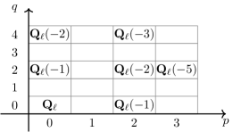
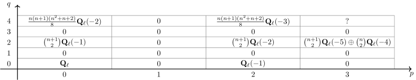
Recall that the -entry of the -sheet of the Leray spectral sequence of is by Proposition 2.8; denote this entry by . We compute many entries on the -sheet and list the nonzero results in Figure 2, from which the theorem follows directly. The special case of is given in Figure 1. All computations here are up to semi-simplification.
-
(1)
for all .
-
(2)
for all , .
-
(3)
for all .
-
(4)
and for .
-
(5)
and .
-
(6)
for all and .
∎
Remark 4.12.
4.2. Explicit computations for .
Once one has computed for fixed and for all , , one can in theory apply Proposition 2.8 and Theorem 3.2 to determine . In this subsection, we detail the results of this process for .
Lemma 4.13.
The local systems on are
Using Lemma 4.13, we can compute all entries of the -page of the Leray spectral sequence for . As always, the following results are up to semi-simplification.
Lemma 4.14.
For , , , , and all ,
For , ,
For , ,
For ,
Proof.
By the usual argument, we obtain the following theorem using these preliminaries.
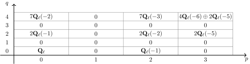
Theorem 4.16.
The cohomology of the second fiber power of the universal abelian surface is given by
up to semi-simplification.
Proof.

5. Cohomology of
In this section, we compute . As opposed to Section 4, we show that the cohomology in fixed degree stabilizes as increases and explicitly give the computations for small degree. Afterwards, we give a complete description of the cohomology for the case . For brevity, we will often drop the constant coefficients if the context is clear, writing instead of .
5.1. Computations for general .
Let and . Let be an abelian surface. For all , the symmetric group acts on by permuting the coordinates, which induces an action of on . The -action on is not free but this is not a problem in the context of stacks. On the other hand,
by the Künneth formula.
Lemma 5.1.
There are isomorphisms of local systems
Proof.
For any abelian surface , there is an isomorphism by the Hochschild–Serre spectral sequence for . For any , let be the sum of all products with which occur in reversed order in the sequence . The induced action of on is then given by
for all with as described in [Mac62]. For example if is a transposition, then which encodes the fact that is a graded commutative ring with respect to the cup product and that for any with for some for all , the cup product corresponds to the simple tensor under the Künneth isomorphism. There is a relationship between , , and which encodes the fact that acts on ; we refer the reader to [Mac62, (1.1)-(1.3)] for more properties of the polynomials since we do not use any of them explicitly in this proof.
There is a projection given by averaging. For each fixed with and , consider the -subrepresentation
The summand corresponding to above can be written as with . For any simple tensor in , it is straightforward to check that . Because is spanned over by such simple tensors and for all , the image is spanned by the images of simple tensors . Therefore, restricted to is surjective onto with kernel .
For a transposition with , observe that
This implies that for ,
and for ,
Combining all of the above,
Therefore, we have proven the desired isomorphisms on the level of -representations. To determine the structure as -representations and as local systems, we add in appropriate Tate twists as in the proofs of Lemma 3.1 and 4.1. ∎
Lemma 5.2.
For fixed , stabilizes for up to semi-simplification.
Proof.
Fix . For each , consider the set
If , then there is a bijection given by sending each . Using this bijection and the fact that for any , compute for all that
By Lemma 5.1 and the above computation, there is an isomorphism of local systems
for all .
Up to semi-simplification,
where the first equality follows by Proposition 2.8 and the second equality follows by the first part of the proof which shows that as local systems,
for all such that . ∎
For small , this simplifies the computations for the local systems .
Proposition 5.3.
For all ,
For all ,
For all ,
For all ,
For all ,
Proof.
The necessary facts from the representation theory of are Lemma 4.2, Lemma 4.3, and [FH04, Exercise 16.11] which says that for any . Applying these facts to the direct sum given by Lemma 5.1 gives the decomposition into irreducible -representations as claimed. Finally, add appropriate Tate twists as in the proof of Lemma 3.1.
As an example, we work out the computation for for explicitly. For , the tuples satisfying and are
Lemma 5.1 gives
Decompose each summand (as -representations) into a direct sum of irreducible representations:
Collect all the terms above to see that as -representations,
as claimed. Now add in Tate twists to the local systems corresponding to the appropriate -representations as in the proof of Lemma 3.1. ∎
Proposition 5.3 provides the inputs to the computation of the cohomology of in the same way as in Sections 3 and 4.
Theorem 1.3.
For all for even and for all for odd,
up to semi-simplification.
Proof.
Denote the -entry on the -sheet of the Leray spectral sequence (given by Proposition 2.8) of by . This spectral sequence degenerates on the -page. Applying Proposition 5.3 and Corollary 3.4 yields for and , , , which we record in Figure 4. Observe also that for all if is odd or if by Theorem 3.2. The theorem now follows directly. ∎
5.2. Explicit computations for .
We compute completely. We first need the following.
Lemma 5.4.
There are isomorphisms of local systems
Proof.
This is a direct computation using Lemma 5.1. ∎
As usual, we want to compute for all , . With Lemma 5.4, this process is completely analogous to that of Sections 3 and 4. Therefore, we list the results below and omit the explanations.
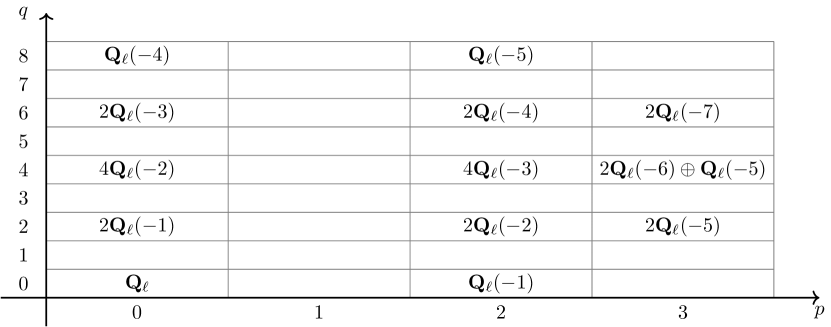
Theorem 5.5.
The cohomology of is given by
up to semi-simplification.
Proof.
Remark 5.6.
Note for all , the term in the spectral sequence for for remain stable and are given in the corresponding entries in Figure 5.
6. Arithmetic Statistics
In this section, we apply the cohomological results of the previous sections to obtain arithmetic statistics results about abelian surfaces over finite fields. In Section 6.2 we point out that the techniques of this paper can be applied to give arithmetic statistics about abelian surfaces with an ordered basis of its -torsion given the cohomology of local systems of , and apply the conjectural formulas ([BFvdG08]) in the case as an example.
Given the étale cohomology of a variety over a finite field , one can use the Grothendieck–Lefschetz trace formula to immediately deduce the number of -points on the variety. Even though the spaces studied in this paper are not varieties but rather algebraic stacks, there is fortunately an applicable generalization, the Grothendieck–Lefschetz–Behrend trace formula, which gives the groupoid cardinality of their -points.
Definition 6.1.
Let be a groupoid. The groupoid cardinality is defined as
The following definition is necessary in order to state the Grothendieck–Lefschetz–Behrend trace formula.
Definition 6.2.
Let be a smooth Deligne–Mumford stack of finite type over . Let be the smooth site associated to . The arithmetic Frobenius acting on is denoted by . The action of on is multiplication by . For any , the action of on is multiplication by .
Remark 6.3.
For Deligne–Mumford stacks, the étale and smooth cohomology of abelian sheaves coincide: the étale and smooth cohomology of an abelian sheaf on schemes coincide by [Sta21, Lemma 03YY] and so the same holds for Deligne–Mumford stacks by étale descent since such stacks admit étale covers by schemes. All stacks in this section are Deligne–Mumford stacks over finite fields (or their algebraic closures ) of any characteristic (see Section 2.1). We will omit the distinction and just write for étale (or smooth) cohomology of .
The main tool of this section is the following trace formula.
Theorem 6.4 (Grothendieck–Lefschetz–Behrend trace formula, [Beh93, Theorem 3.1.2]).
Let be a smooth Deligne–Mumford stack of finite type and constant dimension over the finite field . Then
6.1. Applying the Grothendieck–Lefschetz–Behrend trace formula.
In this subsection, we apply the trace formula (Theorem 6.4) to deduce corollaries of the cohomological results of the previous sections. Although all cohomology computations in the previous sections are only up to semi-simplification, the trace of a linear operator does not change under semi-simplification. Therefore, we apply the trace formula (Theorem 6.4) to the semi-simplification without making this distinction.
Recall that the interpretation of the -points of each stack in question is given in Section 2.1. This first count is well-known, but we list it below for completeness.
Theorem 6.5.
Proof.
The point counts in the rest of this section are new to the best of our knowledge.
Theorem 6.6.
Proof.
We can also piece together the partial information we have about and to give an approximation of and , for fixed and asymptotic in .
Theorem 6.7.
For all ,
For ,
and for all ,
Proof.
By Theorem 2.5, for all and ,
and so for any such that ,
For any and or , this estimate, the trace formula (Theorem 6.4), the properties of the Leray spectral sequence for (Proposition 2.8), and Proposition 4.10 imply
For , applying Theorem 1.2 with gives
and for , the same computation using Theorem 1.3 with gives
and with , gives
Finally, we note that it is possible to compute the exact value of analogously to the calculation of in Theorem 6.6 but we omit it for brevity. ∎
These point counts imply the arithmetic statistics results outlined in Section 1 which we discuss for the remainder of this subsection.
Lemma 6.8.
Define a probability measure on by
for each -isomorphism class . For fixed , the expected value of the number of -points on th powers of abelian surfaces with respect to this probability measure is
Similarly, the expected value of the groupoid cardinality of is
Proof.
Consider a representative abelian surface in a fixed -isomorphism class and let or . There is an action of on . For any , its -isomorphism class is precisely its orbit under the action of . Let denote the stabilizer of in the group . Then the automorphism group of the pair is and the automorphism group of is ; this is a direct product because the action of and on commute.
Let if and if . Let denote the orbit of in under the action of . The contribution of (and its corresponding fiber ) to the expected value is
where the first equality follows from the orbit-stabilizer theorem and the second follows from the fact that the groupoid cardinality of is . ∎
Lemma 6.8 and the results of this section immediately imply the statistics given in Section 1; we restate them here for convenience.
Corollary 1.4.
The expected number of -points on abelian surfaces defined over is
Because for all abelian surfaces , the following corollary gives asymptotics for all moments of as well as the exact second moment.
Corollary 1.5.
The expected value of is
and for all ,
Recall that for an abelian surface and any is the set of -tuples defined over as tuples, i.e. the points are permuted by .
Corollary 1.6.
The expected value of for is
For ,
and for all ,
The fact that we have determined the exact value for the second moment means we can calculate the variance of using Corollary 1.4.
Corollary 1.7.
The variance of is
6.2. Level structures.
Let and let be the projection map. For each local system on , we can define local systems on (also denoted ) via pullback by the map . By [Sta21, Lemma 075H], there is an isomorphism of sheaves
Therefore, the decomposition given in Lemma 3.1 also holds for the local systems on , interpreting all local systems as their pullbacks to .
However, the cohomology of local systems on is not yet known in general. In the case , many parts of the Euler characteristics of local systems on are known and there are conjectures for the rest; this is done in [BFvdG08]. Here, we consider the compactly supported Euler characteristics of such local systems, defined
taken in the Grothendieck group of an appropriate category, e.g. the category of mixed Hodge structures or of Galois representations.
Conjecture 6.9 (Bergström–Faber–van der Geer, [BFvdG08, Section 10]).
The compactly supported Euler characteristic of over is given by . The compactly supported Euler characteristic of over is given by .
The cohomology of is also computed in [LW85, Theorem 5.2.1]. Assuming these two calculations and using the Leray spectral sequence of ,
These computations plus a version of the trace formula (Theorem 6.4) for compactly supported cohomology imply that
In particular, note that an -point on corresponds to an abelian surface defined over with an ordered basis of its -torsion defined over . Therefore, careful analysis of the counts and will yield the average number of abelian surfaces over with -torsion defined over and the average number of -points on such abelian surfaces.
Appendix A Tensor Products of Irreducible -Representations
In this appendix we summarize the combinatorial results decomposing tensor products of irreducible -representations into irreducible ones and prove Lemmas 4.2 and 4.3. As usual, we let denote the irreducible -representation corresponding to the partition .
Let be a partition, so that . A Young diagram of shape is an arrangement of left-justified rows of boxes, such that row has -many boxes. A skew shape , where and are both partitions with is the arrangement of rows of boxes given by the Young diagram of shape , with the Young diagram of shape erased. A skew tableau of shape with content is a labeling of a skew shape where -many of the boxes are labeled with the number . Such a tableau is called semi-standard if the labels are nondecreasing along rows and increasing along columns. Given a skew semi-standard tableau of shape with content , we may demand that the concatenation of the reversed rows is a lattice word: list the entries of the tableau from right to left, starting from the top row and working down; for any smaller than the length of this list, the first elements must contain as many entries as it contains entries . For example, consider the tableau on the left in Figure 6; the concatenation of the reversed rows is “1121.” For , the list of the first entries is “112,” and there are more entries labeled “1” than there are “2” in “112” (and of course, more entries labeled “2” than there are “3,” and so on). This is true for all for this concatenation of the reversed rows for this tableau.
Skew semi-standard tableaux whose concatenation of the reversed rows is a lattice word are called Littlewood–Richardson tableaux. For another description of these tableaux, see [FH04, p. 456]. As an example, we give all Littlewood–Richardson tableaux of shape and content in Figure 6. Finally, the Littlewood–Richardson coefficient is the number of Littlewood–Richardson tableaux of shape and content . One important property about Littlewood–Richardson coefficients is that for all partitions . One can see this by applying the Littlewood–Richardson rule ([FH04, (15.23), (A.8)], [KT87, Theorem 1.4.4]) which says that is the multiplicity of in where , , and are the irreducible representations of corresponding to the partitions using the notation of [FH04, Section 15.3].
& \none 1 1
\none 2
1
{ytableau}
\none& \none 1 1
\none 1
2
Let be the set of all partitions. There is a universal character ring (a -algebra defined in [KT87, Section 1.4]) with a -basis ([KT87, Definition 2.1.1, Proposition 2.1.2]). The structure constants of with respect to the -basis are given by Newell–Littlewood numbers:
Theorem A.1 ([Koi89, Theorem 3.1]).
For any ,
with . Here, is a Littlewood–Richardson coefficient, i.e. the number of Littlewood–Richardson tableaux of shape and content . The constants are known as Newell–Littlewood numbers.
There is an algebra homomorphism where is the character ring of called the specialization homomorphism ([KT87, Section 2.2]). If with where is the length of the partition , then , the character of the irreducible -representation corresponding to ([KT87, Proposition 2.2.1]). The images for such that are computed in [KT87, Section 2.4] and outlined below:
If , let denote the number of boxes in the th column of the Young diagram of for all and let be the total number of columns. If there exists for which , then .
Now assume for all . For , define
and define . Under these assumptions, for all . If for some , then . Otherwise, reorder the numbers in decreasing order with
Define for . If then . Otherwise, let be the Young diagram for which is the number of boxes in the th column. Then and
where is the permutation with for all and is the number of indices such that .
With the arithmetic of given in Theorem A.1 and the specialization homomorphism , we are ready to prove Lemmas 4.2 and 4.3. Similarly as in Section 4, we set and if is not a partition, or more specifically if or for some .
Proof of Lemma 4.2.
By Theorem A.1,
with . According to [KT87, p. 509 (1)], the above sum is given by
Applying the specialization homomorphism with [KT87, Proposition 2.2.1] gives
| () |
Now we determine . Compute that
With and ,
which implies that .
The character of the -representation is the product . Therefore, rewriting on the level of -representations proves this lemma. ∎
Proof of Lemma 4.3.
Let . Suppose , , , and are partitions such that ; we first list all possibilities for such partitions , , , and . Throughout this proof, we define and if any of , , or are tuples of nonnegative integers but are not partitions.
Since , , we must have , , and .
Consider . We have with . This forces the three possibilities: (1) and , (2) and , or (3) and .
Next, consider , and the above three possibilities.
-
(1)
If , then a tableau with shape has boxes in the first row and boxes in the second row. In order for the tableau to satisfy the lattice word condition and have the labels be increasing within each row, the entire first row must be labeled . Therefore, the content must satisfy with . Because , this forces two possibilities: or .
Suppose . We count tableau with shape and content . The tableau of shape has one row with two boxes, and the lattice word condition imposes that all boxes of the first row must be labeled . Therefore, there are no such tableau with content . For , see Figure 7 for the unique tableau with shape and content .
-
(2)
If , then a tableau with shape and content must satisfy or . In both cases, such a tableau is the unique tableau with one box.
-
(3)
If , then a tableau with shape and content must satisfy . In this case, such a tableau must be the empty one.
Lastly, consider .
-
(1)
If , , and , then a tableau with shape and content must satisfy . The only such tableau is the empty one.
-
(2)
If , , and or , then a tableau with shape and content must satisfy with . If , then , , or . If , then , , or . In all cases, such a tableau must be the unique one with one box.
-
(3)
If , , and , then a tableau with shape and content must satisfy with . Then is one of
-
(a)
Suppose or . The tableau of shape has one row with two boxes, and the lattice word condition imposes that all boxes of the first row must be labeled . Therefore, there are no such tableau with content .
-
(b)
Suppose . See Figure 7 for the unique tableau of shape and content .
-
(c)
Suppose or . The tableau of shape has two boxes, each on a distinct row. Therefore, there is a unique tableau of this shape with content .
-
(d)
Suppose . The tableau of shape has one row with two boxes, and the lattice word condition imposes that all boxes of the first row must be labeled . Therefore, there are no such tableau with content .
-
(e)
Suppose . The tableau of shape has two boxes, in two rows and one column. Therefore, there is a unique tableau of shape and content .
-
(a)
& \none \none 1
2
In Figure 8, we record the calculations of the Littlewood–Richardson coefficients , , and for partitions , , , and found above such that . Next, we compute for some of the partitions listed in Figure 8. For any subset , the indicator function of is denoted by (cf. Definition 4.6). Recall that if is not a partition, then by definition.
-
(1)
If , then , , and , so
and
-
(2)
If , then , , and , so
and
-
(3)
If , then
-
(a)
, , and or
-
(b)
, , and , so
and
-
(a)
-
(4)
If , then , , and , so
and
-
(5)
If , then , , and , so
and
-
(6)
If , then , , and , so
and
Aside from the six partitions considered above, the remaining partitions such that are for . For such , compute that
With ,
which implies that .
Next, we determine . Compute that
Then for all . Compute that
The values are all distinct and decreasing so compute that
The Young diagram defined by the values is the diagram of the partition . Since the are strictly decreasing, the permutation reordering these terms is trivial. The only index such that is , and so the number of such indices is . Finally, [KT87, Proposition 2.4.1] implies that
We record the results of these calculations of in Figure 8. Recall that if by [KT87, Proposition 2.2.1].
Applying Theorem A.1 and applying the specialization homomorphism with [KT87, Proposition 2.2.1] and the above computations,
The character of the -representation is the product . Therefore, rewriting the above equality on the level of -representations proves this lemma. ∎
References
- [AEK+15] Jeffrey D. Achter, Daniel Erman, Kiran S. Kedlaya, Melanie Matchett Wood, and David Zureick-Brown. A heuristic for the distribution of point counts for random curves over a finite field. Phil. Trans. R. Soc. A., 373, 2015.
- [AHL13] Yves Aubry, Safia Haloui, and Gilles Lachaud. On the number of points on abelian and Jacobian varieties over finite fields. Acta Arithmetica, 160(3):201–241, 2013.
- [Beh93] Kai A. Behrend. The Lefschetz trace formula for algebraic stacks. Invent. Math., 112(1):127–149, 1993.
- [BFvdG08] Jonas Bergström, Carel Faber, and Gerard van der Geer. Siegel modular forms of genus 2 and level 2: cohomological computations and conjectures. Int. Math. Res. Not., 2008(100), 2008.
- [BFvdG14] Jonas Bergström, Carel Faber, and Gerard van der Geer. Siegel modular forms of degree three and the cohomology of local systems. Sel. Math. New Ser., 20:83–124, 2014.
- [CFHS12] Wouter Castryck, Amanda Folsom, Hendrik Hubrechts, and Andrew V. Sutherland. The probability that the number of points on the Jacobian of a genus 2 curve is prime. Proc. London Math. Soc., 104(6):1235–1270, 2012.
- [Das19] Ronno Das. Cohomology of the universal smooth cubic surface. Q. J. Math., to appear, 2019.
- [Del68] Pierre Deligne. Théorème de Lefschetz et critéres de dégénérescence de suites spectrales. Inst. Hautes Études Sci. Publ. Math., 35:259–278, 1968.
- [Del69] Pierre Deligne. Formes modulaires et représentations -adiques. Sém. Bourbaki, 355:139–172, 1969.
- [DGS+14] Chantal David, Derek Garton, Zachary Scherr, Arul Shankar, Ethan Smith, and Lola Thompson. Abelian surfaces over finite fields with prescribed groups. B. Lond. Math. Soc., 46(4):779–792, 2014.
- [Edi00] Dan Edidin. Notes on the construction of the moduli space of curves. In Geir Ellingsrud, William Fulton, and Angelo Vistoli, editors, Recent Progress in Intersection Theory, pages 85–113, Boston, MA, 2000. Birkhäuser Boston.
- [FC90] Gerd Faltings and Ching-Li Chai. Degeneration of Abelian Varieties. Springer-Verlag, 1990.
- [FH04] William Fulton and Joe Harris. Representation Theory: A First Course. Springer, 2004.
- [FvdG04a] Carel Faber and Gerard van der Geer. Sur la cohomologie des systèmes locaux sur les espaces de modules des courbes de genre et des surfaces abéliennes, I. C. R. Acad. Sci. Paris, Ser. I, 338(5):381–384, 2004.
- [FvdG04b] Carel Faber and Gerard van der Geer. Sur la cohomologie des systèmes locaux sur les espaces de modules des courbes de genre et des surfaces abéliennes, II. C. R. Acad. Sci. Paris, Ser. I, 338(6):467–470, 2004.
- [GHT18] Samuel Grushevsky, Klaus Hulek, and Orsola Tommasi. Stable cohomology of the perfect cone toroidal compactification of . J. Reine Angew. Math., 741:211–254, 2018.
- [HT18] Klaus Hulek and Orsola Tommasi. The topology of and its compactifications. In Jan Arthur Christophersen and Kristian Ranestad, editors, Geometry of Moduli, 2018.
- [Ibu12] Tomoyoshi Ibukiyama. Vector valued Siegel modular forms of symmetric tensor weight of small degrees. Comm. Math. Univ. Sancti Pauli, 61:51–75, 2012.
- [Koi89] Kazuhiko Koike. On the decomposition of tensor products of the representations of the classical groups: by means of the universal characters. Adv. Math., 74:57–86, 1989.
- [KT87] Kazuhiko Koike and Itaru Terada. Young-diagrammatic methods for the representation theory of the classical groups of type , , . J. Algebra, 107:466–511, 1987.
- [LW85] Ronnie Lee and Steven H. Weintraub. Cohomology of and related groups and spaces. Topology, 24(4):391–410, 1985.
- [Mac62] I. G. MacDonald. The Poincaré polynomial of a symmetric product. Mathematical Proceedings of the Cambridge Philosophical Society, 58(4):563–568, 1962.
- [Mil80] J. S. Milne. Étale cohomology. Princeton University Press, 1980.
- [Mil08a] J. S. Milne. Abelian varieties (v2.00), 2008. Available at www.jmilne.org/math/.
- [Mil08b] J. S. Milne. Lectures on étale cohomology (v2.10), 2008. Available at www.jmilne.org/math/.
- [Ols12] Martin Olsson. Compactifications of moduli of abelian varieties: an introduction. In Lucia Caporaso, James McKernan, Mircea Mustaţǎ, and Mihnea Popa, editors, Current Developments in Algebraic Geometry, pages 295–348, Cambridge, 2012. Cambridge University Press.
- [Pet15] Dan Petersen. Cohomology of local systems on the moduli of principally polarized abelian surfaces. Pacific J. Math, 275(1):39–61, 2015.
- [Rüc90] Hans-Georg Rück. Abelian surfaces and jacobian varieties over finite fields. Math. Comp., 76(3):351–366, 1990.
- [Ser73] Jean-Pierre Serre. A Course in Arithmetic. Graduate Texts in Mathematics. Springer-Verlag, 1973.
- [Sta21] The Stacks project authors. The stacks project. https://stacks.math.columbia.edu, 2021.
- [vdG11] Gerard van der Geer. Rank one eisenstein cohomology of local systems on the moduli space of abelian varieties. Sci. China Math., 54:1621–1634, 2011.
- [vdG13] Gerard van der Geer. The cohomology of the moduli space of abelian varieties. In Gavril Farkas and Ian Morrison, editors, Handbook of Moduli, Volume I, pages 415–458. International Press and Higher Education Press, 2013.
- [vdG15] Gerard van der Geer. Counting curves over finite fields. Finite Fields Appl., 32:207 – 232, 2015.
- [Wak12] Satoshi Wakatsuki. Dimension formulas for spaces of vector-valued Siegel cusp forms of degree two. J. Number Theory, 132:200–253, 2012.
- [Wat69] William C. Waterhouse. Abelian varieties over finite fields. Ann. Sci. Éc. Norm. Supér., 4(2):521–560, 1969.
- [Wei05] Rainer Weissauer. Four dimensional Galois representations. In Tilouine Jacques, Carayol Henri, Harris Michael, and Vignéras Marie-France, editors, Formes automorphes (II) - Le cas du groupe , number 302 in Astérisque, pages 67–150. Société mathématique de France, 2005.
- [Wei09] Rainer Weissauer. The trace of hecke operators on the space of classical holomorphic siegel modular forms of genus two. arXiv:0909.1744, 2009.
- [XY20] Jiang Wei Xue and Chia Fu Yu. On counting certain abelian varieties over finite fields. Acta Math. Sin.-English Ser., 2020.