Towards a reliable implementation of least-squares collocation for higher-index differential-algebraic equations

Abstract

In this note we discuss several questions concerning the implementation of overdetermined least-squares collocation methods for higher-index differential algebraic equations (DAEs). Since higher-index DAEs lead to ill-posed problems in natural settings, the dicrete counterparts are expected to be very sensitive, what attaches particular importance to their implementation. We provide a robust selection of basis functions and collocation points to design the discrete problem and substantiate a procedure for its numerical solution. Additionally, a number of new error estimates are proven that support some of the design decisions.

1 Introduction

An overdetermined least-squares collocation method for the solution of boundary-value problems for higher-index differential-algebraic equations (DAEs) has been introduced in HMTWW and further investigated in HMT ; HM ; HM1 . A couple of sufficient convergence conditions have been established. Numerical experiments indicate an excellent behavior. Moreover, it is particularly noteworthy that the computational effort is not much more expensive than for standard collocation methods applied to boundary-value problems for ordinary differential equations. However, the particular procedures are much more sensitive, which reflects the ill-posedness of higher-index DAEs. The question of a reliable implemention is almost completely open. The method offers a number of parameters and options whose selection has not been backed up by any theoretical justifications. The present paper is devoted to a first investigation of this topic. We focus on the choice of collocation nodes, the representation of the ansatz function as well as the shape and structure of the resulting discrete problem. We apply various theoretical arguments, among them also new sufficient convergence conditions in Theorems 2.1, 2.2, and 2.3, and report on corresponding systematic comprehensive numerical experiments.

The paper ist organized as follows: Section 2 contains the information concerning the problem to be solved as well as the basics on the overdetermined least-squares approach, and, additionally, the new error estimates. Section 3 deals with the selection and calculation of collocation points and integration weights for the different functionals of interest and Section 4 provides a robust selection of basis of the ansatz space. The resulting discrete least-squares problem is treated in Section 5, a number of experiments is reported. The more detailed structur of the discrete problem is described in the Appendix. We conclude with Section 6, which contains a summary and further comments.

The algorithms have been implemented in C++11. All computations have been performed on a laptop running OpenSuSE Linux, release Leap 15.1, the GNU g++ compiler (version 7.5.0) GCC , the Eigen matrix library (version 3.3.7) EigenLib , SuiteSparse (version 5.6.0) DavisSS , in particular its sparse QR factorization SPQR , Intel® MKL (version 2019.5-281), all in double precision with a rounding unit of $\epsilon_{\textrm{mach}}\approx 2.22\times 10^{-16}$. The code is optimized using the level -O3.

2 Fundamentals of the problem and method

Consider a linear boundary-value problem for a DAE with properly involved derivative,

$$A(t)(Dx)^{\prime}(t)+B(t)x(t) =q(t),\quad t\in[a,b],$$ (1)

$$G_{a}x(a)+G_{b}x(b) =d.$$ (2)

with $[a,b]\subset\mathbb{R}$ being a compact interval, $D=[I\;0]\in\mathbb{R}^{k\times m}$, $k<m$, with the identity matrix $I\in\mathbb{R}^{k\times k}$. Furthermore, $A(t)\in\mathbb{R}^{m\times k}$, $B(t)\in\mathbb{R}^{m\times m}$, and $q(t)\in\mathbb{R}^{m}$ are assumed to be sufficiently smooth with respect to $t\in[a,b]$. Moreover, $G_{a},G_{b}\in\mathbb{R}^{l\times m}$. Thereby, $l$ is the dynamical degree of freedom of the DAE, that is, the number of free parameters which can be fixed by initial and boundary conditions. Unlike regular ordinary differential equations (ODEs) where $l=k=m$, for DAEs it holds that $0\leq l\leq k<m$, in particular, $l=k$ for index-one DAEs, $l<k$ for higher-index DAEs, and $l=0$ can certainly happen.

Supposing accurately stated initial and boundary conditions, index-one DAEs yield well-posed problems in natural settings and can be numerically treated quite well similarly as ODEs LMW . In contrast, in the present paper, we are mainly interested in higher-index DAEs which lead to essentially ill-posed problems even if the boundary conditions are stated accurately CRR ; LMW ; HMT . The tractability index and projector-based analysis serve as the basis for our investigations. We refer to CRR for a detailed presentation and to LMW ; Mae2014 ; HMT for corresponding short sketches.

We assume that the DAE is regular with arbitrarily high index $\mu\in\mathbb{N}$ and the boundary conditions are stated accurately so that solutions of the problem (1)-(2) are unique. We also assume that a solution $x_{\ast}:[a,b]\rightarrow\mathbb{R}^{m}$ actually exists and is sufficiently smooth.

For the construction of a regularization method to treat an essentially ill-posed problem a Hilbert space setting of the problem is most convenient. For this reason, as in HMTWW ; HMT ; HM , we apply the spaces

$$H_{D}^{1} :=H_{D}^{1}((a,b),\mathbb{R}^{m})=\{x\in L^{2}((a,b),\mathbb{R}^{m}):Dx\in H^{1}((a,b),\mathbb{R}^{k})\},$$

$$L^{2} :=L^{2}((a,b),\mathbb{R}^{m}),$$

which are suitable for describing the underlying operators. In particular, let $\mathcal{T}:H_{D}^{1}\rightarrow L^{2}\times\mathbb{R}^{l}$ be given by

$$(\mathcal{T}x)(t)= \left[\begin{array}[]{c}A(t)(Dx)^{\prime}(t)+B(t)x(t)\\ G_{a}x(a)+G_{b}x(b)\end{array}\right].$$ (5)

Then the boundary-value problem can be described by $\mathcal{T}x=(q,d)^{T}$.

For $K>0$, let $\mathfrak{P}_{K}$ denote the set of all polynomials of degree less than or equal to $K$. Next, we define a finite dimensional subspace $X_{\pi}\subset H_{D}^{1}$ of piecewise polynomial functions which should serve as ansatz space for the least-squares approximation: Let the partition $\pi$ be given by

$$\pi:\quad a=t_{0}<t_{1}<\cdots<t_{n}=b,$$ (6)

with the stepsizes $h_{j}=t_{j}-t_{j-1}$, $h=\max_{1\leq j\leq n}h_{j}$, and $h_{min}=\min_{1\leq j\leq n}h_{j}$.

Let $C_{\pi}([a,b],\mathbb{R}^{m})$ denote the space of piecewise continuous functions having breakpoints merely at the meshpoints of the partition $\pi$. Let $N\geq 1$ be a fixed integer. Then, we define

$$X_{\pi} =\{x\in C_{\pi}([a,b],\mathbb{R}^{m}):Dx\in C([a,b],\mathbb{R}^{k}),$$

$$x_{\kappa}\lvert_{[t_{j-1},t_{j})}\in\mathfrak{P}_{N},\,\kappa=1,\ldots,k,\quad x_{\kappa}\lvert_{[t_{j-1},t_{j})}\in\mathfrak{P}_{N-1},\,\kappa=k+1,\ldots,m,\;j=1,\ldots,n\}.$$ (7)

The continuous version of the least-squares method reads: Find an $x_{\pi}\in X_{\pi}$ which minimizes the functional

$$\Phi(x)=\|\mathcal{T}x\|^{2}=\int_{a}^{b}|A(t)(Dx)^{\prime}(t)+B(t)x(t)-q(t)|^{2}{\rm d}t+|G_{a}x(a)+G_{b}x(b)-d|^{2}.$$ (8)

It is ensured by (HMT, , Theorem 4.1) that, for all sufficiently fine partitions $\pi$ with bounded ratios $1\leq h/h_{min}\leq\rho$, $\rho$ being a global constant, there exists a unique solution $x_{\pi}\in X_{\pi}$ and the inequality

$$\|x_{\pi}-x_{\ast}\|_{H_{D}^{1}}\leq Ch^{N-\mu+1}$$ (9)

is valid. The constant $C\in\mathbb{R}$ depends on the solution $x_{*}$, the degree $N$, and the index $\mu$, but it is independent of $h$. If $N>\mu-1$ then (9) apparently indicates convergence $x_{\pi}\xrightarrow{h\rightarrow 0}x_{*}$ in $H_{D}^{1}$.

At this place it is important to mention that, so far, we are aware of only sufficient conditions of convergence and the error estimates may not be sharp. Not only more practical questions of implementation are open, but also several questions about the theoretical background. We are optimistic that much better estimates are possible since the results of the numerical experiments have performed impressively better than theoretically expected till now.

The following theorem can be understood as a specification of (HMT, , Theorem 4.1) by a more detailed description of the ingredients of the constant C, in particular, now the role of $N$ is better clarified, which could well be important for the practical realization. In particular, it suggests that smooth problems could perhaps be solved better with large N and coarser partitions.

Theorem 2.1

Let the DAE (1) be regular with index $\mu\in\mathbb{N}$ and let the boundary condition (2) be accurately stated. Let $x_{*}$ be a solution of the boundary value problem (1)–(2), and let $A,B,q$ and also $x_{*}$ be sufficiently smooth.

Let $N\geq 1$ and all partitions $\pi$ be such that $h/h_{min}\leq\rho$, with a global constant $\rho$. Then, for all such partitions with sufficiently small $h$, the estimate (9) is valid with

$$C=\frac{N!}{(2N)!\sqrt{2N+1}}C_{N}C_{*}\rho^{\mu-1}C_{data},$$

where

$$C_{\ast} =\max\{\|x_{\ast}^{(N)}\|_{\infty},\|x_{\ast}^{(N+1)}\|_{\infty}\}(m+4k(b-a)^{3})^{1/2},$$

$$C_{data} \quad\text{is independent of $N$ and $h$, it depends only on the data }\;A,D,B,G_{a},G_{b},$$

and $C_{N}$ is a rather involved function of $N$. In particular, there is an integer $K$ with $N\leq K\leq 2(\mu-1)+N$ such that, for $N\rightarrow\infty$, $C_{N}$ does not grow faster than $K^{2(\mu-1)}$. If $A$ and $B$ are constant, it holds $K=N$.

At this place it should be mentioned that estimate Robbins55

$$\sqrt{2\pi N}\left(\frac{N}{e}\right)^{N}e^{1/(12N+1)}\leq N!\leq\sqrt{2\pi N}\left(\frac{N}{e}\right)^{N}e^{1/(12N)},$$

or its slightly less sharp version,

$$\sqrt{2\pi N}\left(\frac{N}{e}\right)^{N}\leq N!\leq\sqrt{2\pi N}\left(\frac{N}{e}\right)^{N}e^{1/12}$$

allow the growth estimate $\frac{N!}{(2N)!}\leq\sqrt{\pi N}e^{1/6}\frac{1}{N!}\frac{1}{4^{N}}$, thus

$$C \leq\sqrt{\pi N}e^{1/6}\frac{1}{N!}\frac{1}{4^{N}\sqrt{2N+1}}C_{N}C_{*}\rho^{\mu-1}C_{data}\leq\sqrt{\frac{\pi}{2}}\,e^{1/6}\frac{1}{N!}\frac{1}{4^{N}}C_{N}C_{*}\rho^{\mu-1}C_{data}$$

$$\leq\frac{1}{N!}\frac{1}{4^{N}}C_{N}C_{*}\rho^{\mu-1}\sqrt{\frac{\pi}{2}}e^{1/6}C_{data}.$$ (10)

However, it should be considered that $C_{N}$ and $C_{*}$ also depend on $N$.

Proof

We apply the estimate HMT

$$\|x_{\pi}-x_{\ast}\|_{H_{D}^{1}}\leq\frac{\|\mathcal{T\|\alpha_{\pi}}}{\gamma_{\pi}}+\alpha_{\pi},$$

in which the approximation error $\alpha_{\pi}$ and the instability threshold $\gamma_{\pi}$ are given by

$$\alpha_{\pi}=\inf_{x\in X_{\pi}}\|x-x_{\ast}\|_{H_{D}^{1}},\quad\gamma_{\pi}=\inf_{x\in X_{\pi},x\neq 0}\frac{\|\mathcal{T}x\|}{\|x\|_{H_{D}^{1}}}.$$

Owing to (HMT, , Theorem 4.1), there is a constant $c_{\gamma}>0$ independent of $\pi$ so that the instability threshold $\gamma_{\pi}$ satisfies the inequality

$$c_{\gamma}h_{min}^{\mu-1}\leq\gamma_{\pi}\leq\lVert\mathcal{T}\rVert,$$

for all partitions with sufficiently small $h$. This leads to

$$\|x_{\pi}-x_{\ast}\|_{H_{D}^{1}}\leq\frac{\alpha_{\pi}}{\gamma_{\pi}}(\|\mathcal{T}\|+\gamma_{\pi})\leq 2\frac{\alpha_{\pi}}{\gamma_{\pi}}\|\mathcal{T}\|.$$

Choosing $N$ interpolation points $\rho_{i}$ with

$$0 <\rho_{1}<\cdots<\rho_{N}<1,$$ (11)

$$\tilde{\omega}(\rho) =(\rho-\rho_{1})\cdots(\rho-\rho_{N}),$$

the approximation error can be estimated by straightforward but elaborate computations by constructing $p_{*}\in X_{\pi}$ such that $p_{*,s}^{\prime}(t_{j-1}+\rho_{i}h_{j})=x_{*,s}^{\prime}(t_{j-1}+\rho_{i}h_{j})$, $p_{*,s}(a)=x_{*,s}(a)$, $s=1,\ldots,k$, $p_{*,s}(t_{j-1}+\rho_{i}h_{j})=x_{*,s}(t_{j-1}+\rho_{i}h_{j})$, $s=k+1,\ldots,m$, $i=1,\ldots,N$, $j=1,\ldots,n$, and regarding $\alpha_{\pi}\leq\|p_{*}-x_{\ast}\|_{H_{D}^{1}}$. One obtains

$$\alpha_{\pi} \leq\frac{h^{N}}{N!}\lVert\tilde{\omega}\rVert_{L^{2}(0,1)}C_{\ast},$$ (12)

$$\quad C_{\ast}=\max\{\|x_{\ast}^{(N)}\|_{\infty},\|x_{\ast}^{(N+1)}\|_{\infty}\}(m+4k(b-a)^{3})^{1/2}.$$

Turning to shifted Gauss-Legendre nodes that minimize $\lVert\tilde{\omega}\rVert_{L^{2}(0,1)}$ we obtain

$$\lVert\tilde{\omega}\rVert_{L^{2}(0,1)}=\frac{(N!)^{2}}{(2N)!\sqrt{2N+1}}.$$

To verify this, we consider the polynomial

$$\omega(t)=2^{N}\tilde{\omega}\bigg{(}\frac{t+1}{2}\bigg{)}=(t-t_{1})\cdots(t-t_{N})$$

with zeros $t_{j}=2\rho_{j}-1$, $j=1,\ldots,N$, which is nothing else but the standard Legendre polynomial with leading coefficient one. Using the Rodrigues formula and other arguments from (HaemHoff91, , Section 5.4), one obtains

$$\lVert\omega\rVert_{L^{2}(-1,1)}=2^{N+\frac{1}{2}}\frac{(N!)^{2}}{(2N)!\sqrt{2N+1}}.$$

Finally, shifting back to the interval $(0,1)$ leads to $\lVert\tilde{\omega}\rVert_{L^{2}(0,1)}=2^{-(N+\frac{1}{2})}\lVert\omega\rVert_{L^{2}(-1,1)}$.

Thus we have

$$\alpha_{\pi}\leq\frac{h^{N}}{N!}\frac{(N!)^{2}}{(2N)!\sqrt{2N+1}}C_{\ast}=h^{N}\frac{N!}{(2N)!\sqrt{2N+1}}C_{\ast}.$$ (13)

Next, a careful review of the proof of (HMT, , Theorem 4.1 (a)) results in the representation (in terms of HMT )

$$\frac{1}{c_{\gamma}} =12c_{Y}\sqrt{g_{\mu-1}}=12c_{Y}\sqrt{d_{1,\mu-1}c^{*}_{\mu-1}\lVert D\mathcal{L}_{\mu-1}\rVert^{2}_{\infty}}$$

$$=12c_{Y}\sqrt{2}\lVert D\Pi_{0}Q_{1}\cdots Q_{\mu-1}D^{+}\rVert_{\infty}\lVert D\mathcal{L}_{\mu-1}\rVert_{\infty}\sqrt{c^{*}_{\mu-1}}.$$

The factors $\lVert D\Pi_{0}Q_{1}\cdots Q_{\mu-1}D^{+}\rVert_{\infty}$ and $\lVert D\mathcal{L}_{\mu-1}\rVert_{\infty}$ depend only on the data $A,D,B$, likewise the bound $c_{Y}$ introduced in (HMT, , Proposition 4.3).

In contrast, the term $c^{*}_{\mu-1}$ depends additionally on $N$ besides the problem data. Let $K$ denote the degree of the auxiliary polynomial $q_{\mu-1}=\mathfrak{A}_{\mu-1}(Dp)^{\prime}+\mathfrak{B}_{\mu-1}p,\;p\in X_{\pi}$ in the proof of (HMT, , Theorem 4.1). Then we have $N\leq K\leq N+2(\mu-1)$ and, by (HMT, , Lemma 4.2), $c_{\mu-1}^{*}=4^{\mu-1}\lambda_{K}\cdots\lambda_{K-\mu+2}$, where each $\lambda_{S}>0$ is the maximal eigenvalue of a certain symmetric, positive semidefinite matrix of size $(S+1)\times(S+1)$ (HMTWW, , Lemma 3.3).

Owing to (HMTWW, , Corollary A.3) it holds that $\lambda_{S}\leq\frac{4}{\pi^{2}}S^{4}+O(S^{2})$ for large $S$, and therefore

$$c_{\mu-1}^{*} =4^{\mu-1}\lambda_{K}\cdots\lambda_{K-\mu+2}$$

$$\leq 4^{\mu-1}(\frac{4}{\pi^{2}})^{\mu-1}K^{4}(K-1)^{4}\cdots(K-\mu+2)^{4}+O(K^{4(\mu-1)-1})$$

$$=4^{\mu-1}(\frac{4}{\pi^{2}})^{\mu-1}K^{4(\mu-1)}+O(K^{4(\mu-1)-1})$$

$$\leq 4^{\mu-1}(\frac{4}{\pi^{2}})^{\mu-1}(N+2(\mu-1))^{4(\mu-1)}+O((N+2(\mu-1))^{4(\mu-1)-1}).$$

Finally, letting

$$C_{data}=2\|\mathcal{T}\|12c_{Y}\sqrt{2}\lVert D\Pi_{0}Q_{1}\cdots Q_{\mu-1}D^{+}\rVert_{\infty}\lVert D\mathcal{L}_{\mu-1}\rVert_{\infty},\quad C_{N}=\sqrt{c^{*}_{\mu-1}},$$

we are done. ∎

Observe that, for smooth problems, any fixed sufficiently fine partition $\pi$, and $N\rightarrow\infty$, the growth rate of the error $\lVert x_{\pi}-x_{*}\rVert_{H^{1}_{D}}$ is not greater than that of

$$C_{*}h^{N}\frac{(N+2(\mu-1))^{2(\mu-1)}}{4^{N}N!}=C_{*}\left(\frac{h}{4}\right)^{N}\frac{(N+2(\mu-1))^{2(\mu-1)}}{N!}$$ (14)

and, for constant matrix function $A$ and $B$,

$$C_{*}h^{N}\frac{N^{2(\mu-1)}}{4^{N}N!}=C_{*}\left(\frac{h}{4}\right)^{N}\frac{N^{2(\mu-1)}}{N!}.$$ (15)

Remember that $C_{*}$ is a function of $N$.

Remark 1

The specific error estimation provided in HMTWW for the case of DAEs in Jordan chain form on equidistant grids may provide some further insight in the behavior of the instability threshold $\gamma_{\pi}$. It is shown that

$$\gamma_{\pi}\geq\bar{C}_{\mu}\left(\frac{h}{\sqrt{\lambda_{N}}}\right)^{\mu-1}$$

holds true for sufficiently small $h$ where $\bar{C}_{\mu}$ is a moderate constant depending only on $\mu$ (HMTWW, , Theorem 3.6). This leads to the dominant error term

$$\frac{\alpha_{\pi}}{\gamma_{\pi}}\leq\frac{C_{\ast}}{\bar{C}_{\mu}}\sqrt{\frac{\pi}{2}}e^{1/6}\frac{1}{2^{2N}}\frac{\lambda_{N}^{\frac{\mu-1}{2}}}{N!}h^{N-\mu+1}=\frac{1}{\bar{C}_{\mu}}\sqrt{\frac{\pi}{2}}e^{1/6}\frac{1}{h^{\mu-1}}C_{\ast}\left(\frac{h}{4}\right)^{N}\frac{\lambda_{N}^{\frac{\mu-1}{2}}}{N!},$$

indicating again that, for smooth problems it seems reasonable to calculate with larger N and coarse partitions. Moreover, for sufficiently small $\frac{h}{\sqrt{\lambda_{N}}}$, the estimation $\lambda_{N}\leq\frac{4}{\pi^{2}}N^{4}+O(N^{2})$ becomes valid (HMTWW, , Remark 3.4), and hence the growth characteristic (15) for large $N$ is confirmed once more. ∎

The functional values $\Phi(x)$, which are needed when minimizing for $x\in X_{\pi}$, cannot be evaluated exactly and the integral must be discretized accordingly. Taking into account that the boundary-value problem is ill-posed in the higher index case $\mu>1$, perturbations of the functional may have a serious influence on the error of the approximate least-squares solution or even prevent convergence towards the solution $x_{\ast}$. Therefore, careful approximations of the integral in $\Phi$ are required. We discuss the following three options:

$$\Phi_{\pi,M}^{C}(x)=\sum_{j=1}^{n}\frac{h_{j}}{M}\sum_{i=1}^{M}|A(t_{ji})(Dx)^{\prime}(t_{ji})+B(t_{ji})x(t_{ji})-q(t_{ji})|^{2}+|G_{a}x(a)+G_{b}x(b)-d|^{2},$$ (16)

$$\Phi_{\pi,M}^{I}(x)=\sum_{j=1}^{n}h_{j}\sum_{i=1}^{M}\gamma_{i}|A(t_{ji})(Dx)^{\prime}(t_{ji})+B(t_{ji})x(t_{ji})-q(t_{ji})|^{2}+|G_{a}x(a)+G_{b}x(b)-d|^{2},$$ (17)

and

$$\Phi_{\pi,M}^{R}(x)=\sum_{j=1}^{n}\int_{t_{j-1}}^{t_{j}}\left|\sum_{i=1}^{M}l_{ji}(t)(A(t_{ji})(Dx)^{\prime}(t_{ji})+B(t_{ji})x(t_{ji})-q(t_{ji}))\right|^{2}{\rm d}t\\ +|G_{a}x(a)+G_{b}x(b)-d|^{2},$$ (18)

in which from the DAE (1) and $x\in X_{\pi}$ only data at the points

$$t_{ji}=t_{j-1}+\tau_{i}h_{j},\quad i=1,\ldots,M,\;j=1,\ldots,n,$$

are included, with

$$0\leq\tau_{1}<\cdots<\tau_{M}\leq 1.$$ (19)

In the last functional $\Phi_{\pi,M}^{R}$ Lagrange basis polynomials appear, i.e.,

$$l_{ji}(t)=\frac{\prod_{\begin{subarray}{c}\kappa=1\\ \kappa\neq i\end{subarray}}^{M}(t-t_{j\kappa})}{\prod_{\begin{subarray}{c}\kappa=1\\ \kappa\neq i\end{subarray}}^{M}(t_{ji}-t_{j\kappa})}=\frac{\prod_{\begin{subarray}{c}\kappa=1\\ \kappa\neq i\end{subarray}}^{M}(\tau-\tau_{\kappa})}{\prod_{\begin{subarray}{c}\kappa=1\\ \kappa\neq i\end{subarray}}^{M}(\tau_{i}-\tau_{\kappa})}=:l_{i}(\tau),\quad\tau=(t-t_{j-1})/h_{j}.$$ (20)

Remark 2

The direct numerical implementation of $\Phi^{R}_{\pi,M}(x)$ with the Lagrangian basis functions includes the use of the mass matrix belonging to such functions. It is well known that this matrix may be very bad conditioned thus leading to an amplification of rounding errors. In connection with the ill-posedness of higher-index DAEs, this may render the numerical solutions useless. The solution of the least-squares problem with $\Phi_{\pi,M}^{I}$ is much less expensive than that with $\Phi^{R}_{\pi,M}$, and in turn, solving system (23)-(24) below for $x\in X_{\pi}$ in a least-squares sense using the (diagonally weighted) Euclidean norm in $\mathbb{R}^{nMm+l}$ according to $\Phi_{\pi,M}^{C}$ is even less computationally expensive than using $\Phi^{I}_{\pi,M}(x)$. ∎

Introducing, for each $x\in X_{\pi}$ and $w(t)=A(t)(Dx)^{\prime}(t)+B(t)x(t)-q(t)$, the corresponding vector $W\in\mathbb{R}^{mMn}$ by

$$W=\left[\begin{array}[]{c}W_{1}\\ \vdots\\ W_{n}\end{array}\right]\in\mathbb{R}^{mMn},\quad W_{j}=h_{j}^{1/2}\left[\begin{array}[]{c}w(t_{j1})\\ \vdots\\ w(t_{jM})\end{array}\right]\in\mathbb{R}^{mM},$$ (21)

we obtain new representations of these functionals, namely

$$\Phi_{\pi,M}^{C}(x)=W^{T}\mathcal{L}^{C}W+|G_{a}x(a)+G_{b}x(b)-d|^{2},$$

$$\Phi_{\pi,M}^{I}(x)=W^{T}\mathcal{L}^{I}W+|G_{a}x(a)+G_{b}x(b)-d|^{2},$$

and

$$\Phi_{\pi,M}^{R}(x)=W^{T}\mathcal{L}^{R}W+|G_{a}x(a)+G_{b}x(b)-d|^{2},$$

whereby the first two formulae are evident, with $\mathcal{L}^{C}=\operatorname{diag}(L^{C}\otimes I_{m},\ldots,L^{C}\otimes I_{m})$, $\otimes$ denoting the Kronecker product, and $L^{C}=M^{-1}I_{M}$ such that finally $\mathcal{L}^{C}=M^{-1}I_{nMm}$, and further, $\mathcal{L}^{I}=\operatorname{diag}(L^{I}\otimes I_{m},\ldots,L^{I}\otimes I_{m})$ and $L^{I}=\operatorname{diag}(\gamma_{1},\ldots,\gamma_{M})$. $L^{C}$ and thus $\mathcal{L}^{C}$ are positive definite. The matrices $L^{I}$ and $\mathcal{L}^{I}$ are positive definite if and only if all quadrature weights are positive.

The formula for $\Phi_{\pi,M}^{R}(x)$ can be established by straightforward evaluations following the lines of (HMTWW, , Section 2.3), in which $\mathcal{L}^{R}=\operatorname{diag}(L^{R}\otimes I_{m},\ldots,L^{R}\otimes I_{m})$, $L^{R}$ is the mass matrix associated with the Lagrange basis functions $l_{i}$, $i=1,\ldots,M$, (20) for the node sequence (19), more precisely,

$$L^{R}=(L_{i\kappa}^{R})_{i,\kappa=1,\ldots,M},\quad L_{i\kappa}^{R}=\int_{0}^{1}l_{i}(\tau)l_{\kappa}(\tau)d\tau.$$ (22)

$L^{R}$ is symmetric and positive definite and, consequently, $\mathcal{L}^{R}$ is so.

We emphasize that the matrices $L^{C},L^{I},L^{R}$ depend only on $M$, the node sequence (19), and the quadrature weights, but do not depend on the partition $\pi$ and $h$ at all.

We set always $M\geq N+1$. Although the nodes (19) serve as interpolation points in the functional $\Phi^{R}_{\pi,M}$, we still call them collocation nodes after HMTWW . It should be underlined here that minimizing each of the above functionals on $X_{\pi}$ can be viewed as a special least-squares method to solve the overdetermined collocation system $W=0$, $G_{a}x(a)+G_{b}x(b))=d$, with respect to $x\in X_{\pi}$, that is in detail, the collocation system

$$A(t_{ji})(Dx)^{\prime}(t_{ji})+B(t_{ji})x(t_{ji}) =q(t_{ji}),\quad j=1,\ldots,M,\quad i=1,\ldots,n,$$ (23)

$$G_{a}x(a)+G_{b}x(b)) =d.$$ (24)

The system (23)-(24) for $x\in X_{\pi}$ becomes overdetermined since $X_{\pi}$ has dimension $mnN+k$, whereas the system consists of $mnM+l\geq mnN+mn+l\geq nmN+m+l>nmN+k+l\geq mnN+k$ scalar equations.

Remark 3

Based on collocation methods for index-1 DAEs, the first thought in HMTWW ; HMT was to turn to the functional $\Phi^{C}_{\pi,M}$ with nodes $0<\tau_{1}<\cdots<\tau_{M}<1$. However, the use of the special discretized norm in these papers for providing convergence results is in essence already the use of the functional $\Phi^{R}_{\pi,M}$.

For a general set of nodes (19), $\Phi^{C}_{\pi,M}$ represents a simple Riemann approximation of the corresponding integral, which has first order of accuracy, only. If, however, the nodes are chosen as those of the Chebyshev intergration, the orders $1,\dots,7$ and $9$ can be obtained for the corresponding number $M$ of nodes (Hildebrand56, , p 349). The marking with the upper index $C$ indicates now that Chebyshev integration formulas are conceivable. As developed in (HaemHoff91, , Section 7.5.2), integration formulas with uniform weights, i.e., Chebyshev formulas, are those where random errors in the function values have the least effect on the quadrature result. This makes these formulas very interesting in our context. However, although a lot of test calculations runs well, we are not aware of convergence statements going along with $\Phi^{C}_{\pi,M}$ so far. ∎

Remark 4

The functional $\Phi^{R}_{\pi,M}$ gets its upper index $R$ from the restriction operator $R_{\pi,M}$ introduced in HM with nodes $0<\tau_{1}<\cdots<\tau_{M}<1$. Note that (HM, , Theorem 2.3) generalizes convergence results from HMTWW ; HMT to a large extend. Theorem 2.2 below allows even any nodes with (19). ∎

Remark 5

The functional $\Phi^{I}_{\pi,M}$ has its upper index $I$ simply from the word integration formula. We will see first convergence results going along with $\Phi^{I}_{\pi,M}$ in Theorem 2.2 below.

Intuitively, it seems reasonable to use a Gaussian quadrature rule for these purposes. However, it is not known if such a rule is most robust against rounding errors and/or other choices of the overall process. ∎

Remark 6

Our approximations are according to the basic ansatz space $X_{\pi}$ discontinuous, with possible jumps at the grid points in certain components. In this respect it does not matter which of our functionals is selected. Since we always have overdetermined systems (23)-(24), it can no longer be expected that all components of the approximation are continuous even for the case $\tau_{1}=0,\tau_{M}=1$. This is an important difference to the classical collocation methods for Index-1 DAEs, which base on classical uniquely solvable linear systems, e.g.,LMW .

Theorem 2.2

Let the DAE (1) be regular with index $\mu\in\mathbb{N}$ and let the boundary condition (2) be accurately stated. Let $x_{*}$ be a solution of the boundary value problem (1)–(2), and let $A,B,q$ and also $x_{*}$ be sufficiently smooth.

Let all partitions $\pi$ be such that $h/h_{min}\leq\rho$, with a global constant $\rho$. Then, with

$$M\geq N+\mu,$$

the following statements are true:

(1)

For sufficient fine partitions $\pi$ and each sequence of arbitrarily placed nodes (19), there exists exactly one $x_{\pi}^{R}\in X_{\pi}$ minimizing the functional $\Phi^{R}_{\pi,M}$ on $X_{\pi}$, and

$$\|x_{\pi}^{R}-x_{\ast}\|_{H_{D}^{1}}\leq C_{R}h^{N-\mu+1}.$$

(2)

For each integration rule related to the interval $[0,1]$, with $M$ nodes (19) and positive weights $\gamma_{1},\ldots,\gamma_{M}$, which is exact for polynomials with degree less than or equal to $2M-2$, and sufficient fine partitions $\pi$, there exists exactly one $x_{\pi}^{I}\in X_{\pi}$ minimizing the functional $\Phi^{I}_{\pi,M}$ on $X_{\pi}$, and $x_{\pi}^{I}=x_{\pi}^{R}$, thus

$$\|x_{\pi}^{I}-x_{\ast}\|_{H_{D}^{1}}\leq C_{R}h^{N-\mu+1}.$$

Since Gauss-Legendre and Gauss-Radau integration rules are exact for polynomials up to degree $2M-1$ and $2M-2$, respectively, with positive weights, they are well suitable here, but Gauss-Lobatto rules do not meet the requirement of Theorem 2.2(2).

Proof

(1): In HM , additionally supposing $0<\tau<\cdots<\tau_{M}<1$, conditions are derived that ensure the existence and uniqueness of $x_{\pi}^{R}$ minimizing $\Phi^{R}_{\pi,M}$ on $X_{\pi}$. It is shown that $x_{\pi}^{R}$ has similar convergence properties as $x_{\pi}$ minimizing $\Phi$ on $X_{\pi}$. Merely the constant $C_{R}$ is slightly larger than $C$ in (9). A further careful check of the proofs in HM shows that the assertion holds also true for $\tau_{1}=0$ and/or $\tau_{M}=1$, possibly with a larger constant $C_{R}$.

(2): For each arbitrary $x\in X_{\pi}$, the expression

$$\theta_{j}(t):=\left|\sum_{i=1}^{M}l_{ji}(t)(A(t_{ji})(Dx)^{\prime}(t_{ji})+B(t_{ji}x(t_{ji})-q(t_{ji}))\right|^{2},\quad t\in(t_{j-1},t_{j}),$$

shows that $\theta_{j}$ is a polynomial with degree less than or equal to $2M-2$, thus

$$\int_{t_{j-1}}^{t_{j}}\theta_{j}(t){\rm dt}=h_{j}\sum_{i=1}^{M}\gamma_{i}\theta_{j}(t_{ji})=h_{j}\sum_{i=1}^{M}\gamma_{i}\left|A(t_{ji})(Dx)^{\prime}(t_{ji})+B(t_{ji}x(t_{ji})-q(t_{ji})\right|^{2}$$

Therefore, it follows that $\Phi_{\pi,M}^{I}(x)=\Phi_{\pi,M}^{R}(x)$, for all $x\in X_{\pi}$, and $\Phi_{\pi,M}^{I}$ coincides with the special functional $\Phi_{\pi,M}^{I}$ having the same nodes. Eventually, (2) is a particular case of (1). ∎

As already emphasized above, until now we are aware of only sufficient convergence conditions, which is, in particular, especially applicable for the size of $M$. So far, often the applications run well with $M=N+1$ and no significant difference to calculations with a larger M was visible, e.g., (HMT, , Section 6) and (HMTWW, , Section 4). Also the experiments in Section 4 below are carried out with $M=N+1$. The following statement for $A$ and $B$ with polynomial entries allows to choose $M$ independently of the index $\mu$ and confirms the choice $M=N+1$ for constant $A$ and $B$.

Theorem 2.3

Let the DAE (1) be regular with index $\mu\in\mathbb{N}$ and let the boundary condition (2) be accurately stated. Let $x_{*}$ be a solution of the boundary value problem (1)–(2), and let $q$ and also $x_{*}$ be sufficiently smooth. Let the entries of $A$ and $B$ be polynomials with degree less than or equal to $N_{AB}$. Let all partitions $\pi$ be such that $h/h_{min}\leq\rho$, with a global constant $\rho$. Then, with

$$M\geq N+1+N_{AB},$$

the following statements are true:

(1)

For sufficient fine partitions $\pi$ and each sequence of arbitrarily placed nodes (19), there exists exactly one $x_{\pi}^{R}\in X_{\pi}$ minimizing the functional $\Phi^{R}_{\pi,M}$ on $X_{\pi}$, and

$$\|x_{\pi}^{R}-x_{\ast}\|_{H_{D}^{1}}\leq C_{R}h^{N-\mu+1}.$$

(2)

For each integration rule of interpolation type related to the interval $[0,1]$, with $M$ nodes (19) and positive weights $\gamma_{1},\ldots,\gamma_{M}$, which is exact for polynomials with degree less than or equal to $2M-2$, and sufficient fine partitions $\pi$, there exists exactly one $x_{\pi}^{I}\in X_{\pi}$ minimizing the functional $\Phi^{I}_{\pi,M}$ on $X_{\pi}$, and $x_{\pi}^{I}=x_{\pi}^{R}$, thus

$$\|x_{\pi}^{I}-x_{\ast}\|_{H_{D}^{1}}\leq C_{R}h^{N-\mu+1}.$$

(3)

If $A$ and $B$ are even constant matrices, for sufficient fine partitions $\pi$ and each sequence of arbitrarily placed nodes (19), there exists exactly one $x_{\pi}^{R}\in X_{\pi}$ minimizing the functional $\Phi^{R}_{\pi,M}$ on $X_{\pi}$, and

$$\|x_{\pi}^{R}-x_{\ast}\|_{H_{D}^{1}}\leq C_{R}h^{\max\{0,N-\mu+1\}}.$$

Proof

(1): This follows from (HM, , Proposition 2.2(iv)) and (HMT, , Theorem 4.1). (2): As in the proof of the previous theorem, this is again a comsequence of (1). (3): The statement is a consequence of (HM, , Proposition 2.2(iv)) and (HMT, , Theorem 4.7).∎

Remark 7

Observe a further interesting feature. Let $A$ and $B$ be constant matrices. Set $N=1$, $M=N+1$. Then, it holds that

$$\Phi_{\pi,M}^{C}(x)=\Phi_{\pi,M}^{R}(x)=\Phi_{\pi,M}^{I}(x),\quad x\in X_{\pi},$$

in which $\Phi_{\pi,M}^{I}$ is associated to the corresponding Gauss-Legendre or Gauss-Radau rules. This follows from the fact that the 2-point Chebyshev integration nodes are just the Gauss-Legendre nodes.

We underline that, by Theorem 2.3(3), the approximate solutions stay bounded also for DAEs with larger index $\mu$, for instance (HMTWW, , Table 6) confirming that for an index four Jordan DAE.∎

Having in mind the implementation of such an overdetermined least-squares collocation, for given partition $\pi$ and a given polynomial degree $N$, a number of parameters and options must be selected:

• basis functions for $X_{\pi}$;

• number $M$ of collocation points and their location $0\leq\tau_{1}<\cdots<\tau_{M}\leq 1$;

• setup and solution of the discrete least-squares problem.

Below we will discuss several issues in this context. The main aim is on implementations being as stable as possible, not necessarily best computational efficiency.

3 Collocation nodes, mass matrix and integration weights

3.1 Collocation nodes for $\Phi^{R}_{\pi,M}$

The functional $\Phi^{R}_{\pi,M}$ in (18) is based on polynomial interpolation using $M$ nodes (19). It seems reasonable to choose these nodes in such a way that, separately on each subinterval $[t_{j-1},t_{j}]$ of the partition, the interpolation error is as small as possible in a certain sense. Without restriction of the generality we can trace back the matter to the interval $[0,1]$.

Consider functions $q\in C([0,1],\mathbb{R}^{m})$ and define the interpolation operator $R_{M}:C([0,1],\mathbb{R}^{m})\rightarrow C([0,1],\mathbb{R}^{m})$ by

$$R_{M}q=\sum_{i=1}^{M}l_{i}q(\tau_{i}),$$

with the Lagrange basis functions (20) such that $(R_{M}q)(\tau_{i})=q(\tau_{i})$, $i=1,\ldots,M$, and $R_{M}q\in Y_{M}$, where $Y_{M}\subset C([0,1],\mathbb{R}^{m})$ is the subspace of all functions whose components are polynomials up to degree $M-1$. Introducing $\omega(\tau)=(\tau-\tau_{1})(\tau-\tau_{2})\cdots(\tau-\tau_{M})$ and using componentwise the divided differences we have the error representation, e.g., (HaemHoff91, , Kapitel 5),

$$q(\tau)-(R_{M}q)(\tau)=\omega(\tau)\,q[\tau_{1},\ldots,\tau_{M},\tau].$$

For smooth functions $q\in C^{M}([0,1],\mathbb{R}^{m})$ it follows that

$$\lVert q-R_{M}q\rVert^{2}_{L^{2}}=\int_{0}^{1}\omega(\tau)^{2}\,\lvert q[\tau_{1},\ldots,\tau_{M},\tau]\rvert^{2}{\rm d\tau}\leq\int_{0}^{1}\omega(\tau)^{2}{\rm d\tau}\frac{m}{(M!)^{2}}\lVert q^{(M)}\rVert^{2}_{\infty}.$$

For the evaluation of $\Phi_{\pi,M}^{R}$ (18), it seems resonable to choose the collocation nodes in such a way that this expression is minimized for all functions $q\in C^{(M)}([0,1],\mathbb{R}^{m})$. The optimal set of nodes is determined by the condition

$$\min_{0\leq\tau_{1}<\cdots<\tau_{M}\leq 1}\|\omega\|_{L^{2}(0,1)}.$$

It is well known that this functional is minimized if the collocation nodes are chosen to be the Gauss-Legendre nodes (HaemHoff91, , Chapter 7.5.1 and 4.5.4).

On the other hand, the best polynomial approximation to a given function $q$ in the $L^{2}$-norm is obtained if the Fourier approximation with respect to the Legendre polynomials is computed. However, to the best of our knowledge, there are no estimations of the interpolation error in $L^{2}((0,1),\mathbb{R}^{m})$ known. However, in the uniform norm and with arbitrary node sequences, for each $q\in C([0,1],\mathbb{R}^{m})$, the estimate

$$\|R_{M}q-q\|_{\infty}\leq(1+\Lambda_{M})\operatorname{dist}_{\infty}(q,Y_{M})$$

holds true where $\operatorname{dist}_{\infty}(q,Y_{M})=\min\{\|q-y\|_{\infty}|y\in Y_{M}\}$ and $\Lambda_{M}$ is so-called Lebesgue constant defined by

$$\Lambda_{M}=\max_{\tau\in[0,1]}\sum_{i=1}^{M}|l_{i}(\tau)|$$

in which $l_{i}$ are again the Lagrange basis functions (20).

The Lebesgue constant $\Lambda_{M}^{L}$ for Gauss-Legendre nodes has the property $\Lambda_{M}^{L}=O(\sqrt{M})$. If instead Chebyshev nodes are used, the corresponding Lebesgue constant $\Lambda_{M}^{C}$ behaves like $\Lambda_{M}^{C}=O(\log M)$ ((FoSl94, , p 206) and the references therein). For uniform polynomial approximations, these nodes are known to be optimal (DeuflHohmann, , Theorem 7.6). Table 1 shows some values for the Lebesgue constants. Note that the Lebesgue constants $\Lambda_{M}^{U}$ for equidistant nodes grow exponentially, see e.g. TrefWeid91 .

Table 1: Lebesgue contants for Chebyshev nodes ($\Lambda_{M}^{C}$), Gauss-Legendre nodes ($\Lambda_{M}^{L}$), Gauss-Lobatto nodes ($\Lambda_{M}^{Lo}$), Gauss-Radau nodes ($\Lambda_{M}^{R}$), and uniform nodes including the boundaries ($\Lambda_{M}^{U}$) and without boundaries ($\Lambda_{M}^{O}$)

$M$	$\Lambda_{M}^{C}$	$\Lambda_{M}^{L}$	$\Lambda_{M}^{Lo}$	$\Lambda_{M}^{R}$	$\Lambda_{M}^{U}$	$\Lambda_{M}^{O}$
5	1.989	3.322	1.636	4.035	2.708	10.375
10	2.429	5.193	2.121	6.348	17.849	204.734
15	2.687	6.649	2.386	8.126	283.211	5107.931
20	2.870	7.885	2.576	9.627	5889.584	138852.138

Remark 8

Computation of nodes and weights for for Gauss-type integration formulae

In the following we will make heavy use of Gauss-Legendre, Gauss-Radau, and Gauss-Lobatto integration nodes and their corresponding weights. Since we do not have them available in tabular form for large $M$ with sufficient accuracy, they will be computed on the fly. A severe concern is the accuracy of the nodes and weights. In the case of Gauss-Legendre integration rules, the computed nodes and weights have been provided by the Gnu Scientific Library routine glfixed.c GSL09 . It makes use of tabulated values for $M=1(1)20$, 32, 64, 96, 100, 128, 256, 512, 1024 with an accuracy of 27 digits. Other values are computed on the fly with an accuracy being a small multiple of the machine rounding unit using an adapted version of the Newton method.

For computing the Gauss-Lobatto nodes and weights, the methods of Michels63 (using the Newton method) as well as Gautschi00b (a variant of the method in GolubWelsch69 ) have been implemented. Table 2 contains some comparisons to the tabulated values in Michels63 that have 20 digits. The method of Michels63 provides slighly more accurate values than that of Gautschi00b . Therefore, the former has been used further on.

We did not find sufficiently accurate tabulated values for the Gauss-Radau nodes and weights. Therefore, the method of Gautschi00a has been implemented. We assume that the results obtained have an accuracy similar to the values for the Gauss-Lobatto nodes and weights using the method in Gautschi00b . ∎

Table 2: Accuracy of the computed nodes and weights of the Gauss-Lobatto integration rules. For each method, the absolute error of the nodes (A), the absolute error of the weights (B), the maximum componentwise relative error of nodes (C) and weights (D) are shown. The machine accuracy (machine epsilon) is $2.22\times 10^{-16}$

$M$	Method ofMichels63				Method of Gautschi00b
	(A)	(B)	(C)	(D)	(A)	(B)	(C)	(D)
6	1.11e-16	1.11e-16	4.73e-16	5.87e-16	1.11e-16	3.33e-16	4.73e-16	9.99e-15
12	1.11e-16	8.33e-17	2.01e-15	6.14e-16	3.33e-16	4.44e-16	6.04e-15	5.86e-14
24	0	3.47e-17	0	9.64e-16	2.22e-16	2.22e-16	8.37e-15	1.23e-13
48	1.11e-16	3.47e-17	3.41e-14	5.23e-15	3.33e-16	1.22e-15	1.71e-13	2.76e-12
96	5.55e-16	2.95e-17	4.73e-16	1.76e-14	4.44e-16	4.44e-16	2.76e-13	4.05e-12

3.2 The mass matrix

In the following, we will make extensive use of Legendre polynomials. For the readers convenience, the necessary properties are collected in Appendix A.1.

Let us turn to $\Phi_{\pi,M}^{R}$ (18) again. A critical ingredient for determining its properties is the mass matrix $L^{R}$ in (22). Denote as before by $l_{i}(\tau)$, $i=1,\ldots,M$, the Lagrange basis functions for the node sequence (19), that is, cf. (20),

$$l_{i}(\tau)=\frac{\prod_{\kappa\neq i}(\tau-\tau_{\kappa})}{\prod_{\kappa\neq i}(\tau_{i}-\tau_{\kappa})}.$$

For evaluating $L^{R}$, we will use the normalized shifted Legendre polynomials $\hat{P}_{\nu}=(2\nu+1)^{1/2}\tilde{P}_{\nu}$ (cf Appendix A.1). Assume the representation

$$l_{i}(\tau)=\sum_{\nu=1}^{M}\alpha_{i\nu}\hat{P}_{\nu-1}(\tau).$$ (25)

A short calculation shows

$$L_{ij}^{R}=\sum_{\lambda=1}^{M}\alpha_{i\lambda}\alpha_{j\lambda}.$$

Letting $a^{i}=(\alpha_{i1},\ldots,\alpha_{iM})^{T}$ we obtain $L_{ij}^{R}=(a^{i})^{T}a^{j}$. Collecting the vectors $a^{i}$ in a matrix $A=(a^{1},\ldots,a^{M})$ it holds $L^{R}=A^{T}A$. The definition of the coefficients $\alpha_{i\nu}$ provides us with $\tilde{V}a^{i}=e^{i}$ where $e^{i}$ denotes the $i$-th unit vector and

$$\tilde{V}=\left[\begin{array}[]{ccc}\hat{P}_{0}(\tau_{1})&\ldots&\hat{P}_{M-1}(\tau_{1})\\ \vdots&&\vdots\\ \hat{P}_{0}(\tau_{M})&\ldots&\hat{P}_{M-1}(\tau_{M})\end{array}\right].$$ (26)

This gives $A=\tilde{V}^{-1}$.

$V=\tilde{V}^{T}$ is a so-called Vandermonde-like matrix Gautschi83 . It is nonsingular under the condition (19) (Stoer89, , Theorem 3.6.11). In Gautschi83 , representations and estimations of the condition number with respect to the Frobenius norm of such matrices are derived. In particular, (Gautschi83, , Table 1) shows impressingly small condition numbers if the collocation nodes are chosen to be the zeros of $\tilde{P}_{M}$, that is the Gauss-Legendre nodes. Moreover, this condition number is optimal among all scalings of the Legendre polynomials Gautschi83 . A consequence of the Christoffel-Darboux formula is that the rows of $\tilde{V}$ are orthogonal for Gauss-Legendre nodes. Thus, we have the representation $\tilde{V}=\mathcal{D}U$ with an orthogonal matrix $U$ and a diagonal matrix $\mathcal{D}$ with positive diagonal entries.

It is known that the Gauss-Legendre nodes are not the very best set of nodes. However, a comparison of Tables 1 and 2 in Gautschi83 as well as (Gautschi11, , Table 4) indicates that the gain of choosing optimal nodes for Legendre polynomials compared to the choice of Gauss-Legendre nodes is rather minor.

In Table 3 we provide condition numbers of $\tilde{V}$ with respect to the Euclidean norm for different choices of nodes. Note that the condition number of $L^{R}$ is the square of that of $\tilde{V}$.

The condition numbers for all Gauss-type and Chebyshev nodes are remarkably small.

Table 3: Spectral condition numbers of the Vandermonde-like matrices for different node choices. The columns represent Gauss-Legendre nodes (GLe), Gauss-Radau nodes (GR), Gauss-Lobatto nodes (GLo), Chebyshev nodes (Ch), Newton-Cotes type nodes including the boundary (cNC) and without the boundary (oNC). An asterisk * indicates an overflow condition

$M$	GLe	GR	GLo	Ch	cNC	oNC
5	1.55e+0	2.79e+0	3.23e+0	2.16e+0	3.76e+0	3.04e+0
10	2.11e+0	3.96e+0	4.28e+0	3.00e+0	2.39e+1	5.23e+1
15	2.57e+0	4.85e+0	5.11e+0	3.66e+0	3.98e+2	1.14e+3
20	2.94e+0	5.60e+0	5.83e+0	4.21e+0	8.62e+3	3.10e+4
50	4.62e+0	8.86e+0	9.00e+0	6.60e+0	1.13e+12	1.97e+13
100	6.52e+0	1.25e+1	1.26e+1	9.32e+0	*	*

3.3 Computation of quadrature weights for general $\Phi^{I}_{\pi,M}$

In oder to apply $\Phi_{\pi,M}^{I}$(17), a numerical quadrature formulae is necessary. For standard nodes sequences (Gauss-Legendre, Gauss-Lobatto, Gauss-Radau) their computation has been described above. However, for general node sequences, the weights must be evaluated. This can be done following the derivations in (Stoer89, , p. 175): Let $\hat{P}_{\nu}(\tau)$ denote the normalized shifted Legendre polynomials as before (cf. Appendix A.1). In particular, it holds then

$$\int_{0}^{1}\hat{P}_{0}(\tau){\rm d}\tau=1,\quad\int_{0}^{1}\hat{P}_{\nu}(\tau){\rm d}\tau=0,\quad\nu=1,2,\ldots$$

For a given function $q\in C[0,1]$, the integral is approximated by the integral of its polynomial interpolation. Using the representation (25) of the Lagrange basis functions we obtain

$$\int_{0}^{1}q(\tau)d\tau \approx\int_{0}^{1}\sum_{i=1}^{M}q(\tau_{i})\sum_{\nu=1}^{M}\alpha_{i\nu}\hat{P}_{\nu-1}(\tau){\rm d}\tau$$

$$=\sum_{i=1}^{M}q(\tau_{i})\sum_{\nu=1}^{M}\alpha_{i\nu}\int_{0}^{1}\hat{P}_{\nu-1}(\tau){\rm d}\tau$$

$$=\sum_{i=1}^{M}q(\tau_{i})\alpha_{i1}.$$

Consequently, for the weights it holds $\gamma_{i}=\alpha_{i1}$, $i=1,\ldots,M$. The definition (25) shows that the vector $\gamma=(\gamma_{1},\ldots,\gamma_{M})^{T}$ of weights fulfills the linear system

$$V\gamma=e^{1}$$

where $V=\tilde{V}^{T}$with $\tilde{V}$ from (26) and $e^{1}=(1,0,\ldots,0)^{T}$ is the first unit vector.

The discussion of the condition number of $V$ shows that we can expect reliable and accurate results at least for reasonable node sequences.

For general node sequences, the weights may become negative. This happens, for example, for uniformly distributed nodes and $M>7$ (Newton-Cotes formulae) (Stoer89, , p. 148). So for $\Phi_{\pi,M}^{I}$, only node sequences leading to positive quadrature weights $\gamma_{i}$ are admitted in order to prevent $L^{I}$ from not being positive definite.

4 Choice of basis functions for the ansatz space $X_{\pi}$

The ansatz space $X_{\pi}$ (7) consists of piecewise polynomials having the degree $N-1$ for the algebraic components and the degree $N$ for the differentiated ones on each subinterval of the partition $\pi$ (6). For collocation methods for boundary value problems for ordinary differential equations this questions has lead to the choice of a Runge-Kutta basis for stability reasons, see BaderAscher . This has been later on also used successfully for boundary value problems for index-1 DAEs AscherSpiteri ; KKPSW ; LMW ; KMPW10 . However, this ansatz makes heavily use of the collocation nodes which are at the same time used as the nodes for the Runge-Kutta basis. In our case, the number $M$ of collocation nodes and the degree $N$ of the polynomials for the differentiated components do not coincide since $M>N$ such that the reasoning applied in the case of ordinary differential equations does not transfer to the least-squares case.

Taking into account the computational expense for solving the discretized system, bases with local support are preferable. Ideally, the support of each basis function consists of only one subinterval of (6). Note that the Runge-Kutta basis has this property. We consider the Runge-Kutta basis and further local basis with orthogonal polynomials. A drawback of this strategy is the fact that the continuity of the piecewise polynomials approximating the differentiated components must be ensured explicitly. This in turn will lead to a discrete least-squares problem with equality constraints. Details can be found in Appendix A.3.

Looking for a local basis we turn to the reference interval $[0,1]$. Once a basis on this reference interval is available it can be defined on any subinterval $(t_{j-1},t_{j})$ by a simple linear transformation.

Assume that $\{p_{0},\ldots,p_{N-1}\}$ is a basis of the set of polynomials of degree less than $N$ defined on the reference interval $[0,1]$. Then, a basis $\{\bar{p}_{0},\ldots,\bar{p}_{N}\}$ for the ansatz functions for the differentiated components is given by

$$\bar{p}_{i}(\rho)=\begin{cases}1,&i=0,\\ \int_{0}^{\rho}p_{i-1}(\sigma){\rm d}\sigma,&i=1,\ldots,N,\quad\rho\in[0,1],\end{cases}$$ (27)

and the transformation to the interval $(t_{j-1},t_{j})$ of the partition $\pi$ (6) yields

$$p_{ji}(t) =p_{i}((t-t_{j-1})/h_{j}),$$

$$\bar{p}_{ji}(t) =h_{j}\bar{p}_{i}((t-t_{j-1})/h_{j}).$$ (28)

Additionally to this transformation, the continuity of the piecewise polynomials must be ensured. This gives rise to the additional conditions

$$\bar{p}_{ji}(t_{j})=\bar{p}_{j+1,i}(t_{j}),\quad i=1,\ldots,N,\quad j=1,\ldots,n-1,$$ (29)

which must be imposed explicitely.

4.1 The Runge-Kutta basis

In order to define the Runge-Kutta basis, let the $N$ interpolation points $\rho_{i}$ with (11) be given. Then, the Lagrange basis functions are chosen,

$$p_{i}(\rho)=\frac{\prod_{\kappa\neq i+1}(\rho-\rho_{\kappa})}{\prod_{\kappa\neq i+1}(\rho_{i}-\rho_{\kappa})},\quad i=0,\ldots,N-1.$$

Remark 9

Note that the interpolation nodes are only used to define the local basis functions. Thus, their selection is completely independent of the choice of collocation nodes. In view of the estimations (12) and (13) and the argumentation there we prefer Gauss-Legendre interpolation nodes. This choice is also supported by Experiments 2 and 5 below.

The numerical computation of $\bar{p}$ is more involved. If not precalculated, the integrals must be available in a closed formula. This can surely be done by expressing the Lagrange basis functions in the monomial representation such that the integration can be carried out analytically. Once these coefficients are known, the evaluation of the values of the basis functions at a given $\rho\in[0,1]$ is easily done using the Horner method. However, this approach amounts to the inversion of the Vandermonde matrix using the nodes (11). This matrix is known to be extremly ill-conditioned. In particular, its condition number grows exponentially with $N$ GaIn88 ; Beckermann00 . Therefore, an orthogonal basis might be better suited. This leads to a representation

$$p_{i}(\rho)=\sum_{\kappa=1}^{N}\alpha_{i\kappa}Q_{\kappa}(\rho)$$ (30)

for some polynomials $Q_{1},\ldots,Q_{N}$. If these polynomials fulfil a three-term recursion, the evaluation of function values can be performed using the Clenshaw algorithm FoxParker68 which is only slightly more expensive than the Horner method. In order to use this approach, the integrals of $p_{0},\ldots,p_{N-1}$ must be easily representable in terms of the chosen basis. Here, the Legendre and Chebyshev polynomials are well-suited (cf below Appendix A.1 and (34) as well as Appendix A.2 and (36)).

4.2 Orthogonal polynomials

A reasonable choice for the basis are orthogonal polynomials. We will consider Legendre polynomials first. A motivation is provided in the following example.

Example 1

Consider the index-1 DAE

$$x=q(t),\quad t\in[0,1].$$

Let $\{\hat{P}_{0},\ldots,\hat{P}_{N-1}\}$ be the normalized shifted Legendre polynomials. Then letting $x=\sum_{i=1}^{N}\alpha_{i}\hat{P}_{i-1}$ for some vector $\alpha=(\alpha_{1},\ldots,\alpha_{N})^{T}$, the least-squares functional

$$\Phi(x)=\int_{0}^{1}(x(t)-q(t))^{2}{\rm d}t$$

corresponding to this DAE is minimized if $\alpha=b$ and $b=(b_{1},\ldots,b_{N})^{T}$ where $b_{i}=\int_{0}^{1}q(t)\hat{P}_{i-1}(t)dt$ which is just the best approximation of the solution in $H_{D}^{1}((0,1),\mathbb{R})=L^{2}((0,1),\mathbb{R})$.

Similar relations hold for the differential equation $x^{\prime}=f$ if the basis functions for the differentiated components are constructed according to (27). Hence, these basis functions seem to qualify well for index-1 DAEs. ∎

The necessary ingredients for the efficient implementation of the Legendre polynomials are collected in Appendix A.1.

Another common choice are Chebyshev polynomials of the first kind. They have been used extensivly in the context of spectral methods because of their excellent approximation properties, cf Fornberg96 ; Trefethen00 , see also DrHatr14 . The relations used for their implementation can be found in Appendix A.2.

4.3 Comparison of different basis representations

The choice of the basis function representations is dominated by the question of obtaining a most robust implementation. The computational complexity of the representations presented above is not that much different such that this aspect plays a minor role.

The check for robustness can be subdivided into two questions:

1. Which representation is most robust locally?

2. Which representation is most robust globally?

In the following experiments, $N$ will be varied. The functional used is $\Phi_{\pi,M}^{R}$. The number of collocation nodes is $M=N+1$. Table 3 motivates the choice of the Gauss-Legendre nodes as collocation nodes. In order to compute the norms of $L^{2}((0,1),\mathbb{R}^{m})$ and $H_{D}^{1}((0,1),\mathbb{R}^{m})$, Gaussian quadrature with $N+2$ integration nodes on each subinterval of $\pi$ is used.

Local behavior of the basis representations

In order to answer the first question, is is reasonable to experiment first with a higher index example that does not have any dynamic components (that is, $l=0$) on a grid $\pi$ consisting only of one subinterval (that is, $n=1$). In that case, we check the ability to interpolate functions and to numerically differentiate them.

For $n=1$, there are no continuity conditions (29) involved. Therefore, the discrete problem becomes a linear least-squares problem. We will solve it by a Householder QR-factorization with column pivoting as implemented in the Eigen library.

The following example is used in HMTWW ; HMT .

Example 2

$$x^{\prime}_{2}(t)+x_{1}(t) =q_{1}(t),$$

$$t\eta x^{\prime}_{2}(t)+x^{\prime}_{3}(t)+(\eta+1)x_{2}(t) =q_{2}(t),$$

$$t\eta x_{2}(t)+x_{3}(t) =q_{3}(t),\quad t\in[0,1].$$

This is an index-3 example with dynamical degree of freedom $l=0$ such that no additional boundary or initial conditions are necessary for unique solvability. We choose the exact solution

$$x_{\ast,1}(t) =e^{-t}\sin t,$$

$$x_{\ast,2}(t) =e^{-2t}\sin t,$$

$$x_{\ast,3}(t) =e^{-t}\cos t$$

and adapt the right-hand side $q$ accordingly. For the exact solution, it holds $\|x_{\ast}\|_{L^{2}((0,1),\mathbb{R}^{3})}\approx 0.673$, $\|x_{\ast}\|_{L^{\infty}((0,1),\mathbb{R}^{3})}=1$, and $\|x_{\ast}\|_{H_{D}^{1}((0,1),\mathbb{R}^{3})}\approx 1.11$.∎

Experiment 1

Robustness of the representation of the Runge-Kutta basis

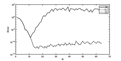
(1)

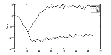
(2)

(3)

Figure 1: Error of the approximate solution in Experiment 1. The abbreviations (M) for the monomial basis, (L) for the Legendre basis, and (C) for the Chebyshev basis are used. The error is measured in the norms of (1) $L^{2}((0,1),\mathbb{R}^{m})$, (2) $L^{\infty}((0,1),\mathbb{R}^{m})$, and (3) $H_{D}^{1}((0,1),\mathbb{R}^{m})$.

In a first experiment we intend to clarify the differences between different representations of the Runge-Kutta basis. The interpolation nodes (11) have been fixed to be the Gauss-Legendre nodes (cf (12)). The Runge-Kutta basis has been represented with respect to the monomial, Legendre, and Chebyshev bases. The results are shown in Figure 1 (see appendix). This test indicates that the monomial basis is much less robust than the others for $N>10$ while the other representations behave very similar. ∎

 

Experiment 2

Robustness of the Runge-Kutta basis with respect to the node sequence

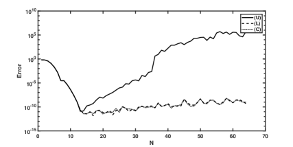
(2)

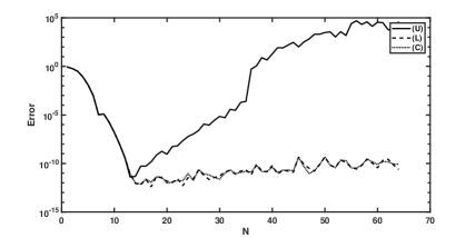
(3)

Figure 2: Error of the approximate solution in Experiment 2. The abbreviations (U) for uniform nodes, (L) for the Gauss-Legendre nodes, and (C) for the Chebyshev nodes are used. The error is measured in the norms of (1) $L^{2}((0,1),\mathbb{R}^{m})$, (2) $L^{\infty}((0,1),\mathbb{R}^{m})$, and (3) $H_{D}^{1}((0,1),\mathbb{R}^{m})$.

In this experiment we are interested in understanding the influence of the interpolation nodes. For that, we compared the uniform nodes sequence to the Gauss-Legendre and Chebyshev nodes. The uniform nodes are given by $\rho_{i}=(i-\frac{1}{2})/N$. In accordance with the results of the previous experiment, the representation of the Runge-Kutta basis in Legendre polynomials has been chosen. The results are shown in Figure 2. Not unexpectedly, uniform nodes are inferior to the other choices at least for $N>13$. On the other hand, there is no significant difference between Gauss-Legendre and Chebyshev nodes. ∎

 

Experiment 3

Robustness of different polynomial representations

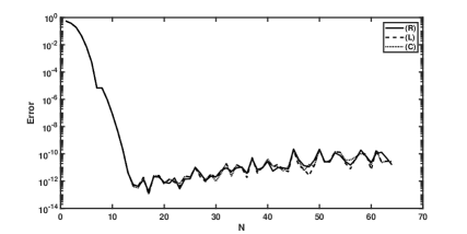
(1)

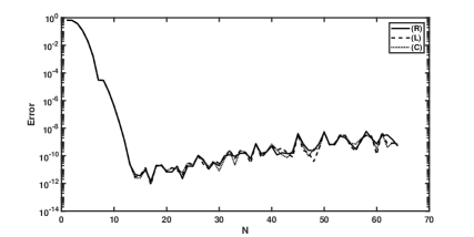
(2)

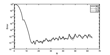
(3)

Figure 3: Error of the approximate solution in Experiment 3. The abbreviations (R) for the Runge-Kutta basis in Legendre representation, (L) for the Legendre basis, and (C) for the Chebyshev basis are used. The error is measured in the norms of (1) $L^{2}((0,1),\mathbb{R}^{m})$, (2) $L^{\infty}((0,1),\mathbb{R}^{m})$, and (3) $H_{D}^{1}((0,1),\mathbb{R}^{m})$.

In this experiment we intend to compare the robustness of different bases. Therefore, we have chosen the Runge-Kutta basis with Gauss-Legendre interpolation nodes, the Legendre polynomials, and the Chebyshev polynomials. The results are shown in Figure 3. All representations show similar behavior. ∎

A general note is in order. The exact solution has approximately the norm 1 in all used norms. The machine accuracy is $\varepsilon_{\textrm{mach}}\approx 2.22\times 10^{-16}$ in all computations. The best accuracy obtained is $10^{-12}$ – $10^{-14}$. Considering that there is a twofold differentiation involved in the problem of the example we would expect a much lower accuracy. This surprising behavior has also been observed in other experiments.

The next example is an index-3 one which has $l=4$ dynamical degrees of freedom. It is the linearized version of an example presented CampbellMoore95 that has also been considered in HMT .

Example 3

Consider the DAE

$$A(Dx(t))^{\prime}+B(t)x(t)=q(t),\quad t\in[0,5],$$

where

$$A=\begin{bmatrix}1&0&0&0&0&0\\ 0&1&0&0&0&0\\ 0&0&1&0&0&0\\ 0&0&0&1&0&0\\ 0&0&0&0&1&0\\ 0&0&0&0&0&1\\ 0&0&0&0&0&0\end{bmatrix},D=\begin{bmatrix}1&0&0&0&0&0&0\\ 0&1&0&0&0&0&0\\ 0&0&1&0&0&0&0\\ 0&0&0&1&0&0&0\\ 0&0&0&0&1&0&0\\ 0&0&0&0&0&1&0\end{bmatrix},$$

and the smooth coefficient matrix

$$B(t)=\begin{bmatrix}0&0&0&-1&0&0&0\\ 0&0&0&0&-1&0&0\\ 0&0&0&0&0&-1&0\\ 0&0&\sin t&0&1&-\cos t&-2\rho\cos^{2}t\\ 0&0&-\cos t&-1&0&-\sin t&-2\rho\sin t\cos t\\ 0&0&1&0&0&0&2\rho\sin t\\ 2\rho\cos^{2}t&2\rho\sin t\cos t&-2\rho\sin t&0&0&0&0\end{bmatrix},\quad\rho=5,$$

subject to the initial conditions

$$x_{2}(0)=1,\quad x_{3}(0)=2,\quad x_{5}(0)=0,\quad x_{6}(0)=0.$$

This problem has the tractability index 3 and dynamical dgree of freedom $l=4$. The right-hand side $q$ has been chosen in such a way that the exact solution becomes

$$x_{\ast,1} =\sin t, x_{\ast,4} =\cos t,$$

$$x_{\ast,2} =\cos t, x_{\ast,5} =-\sin t,$$

$$x_{\ast,3} =2\cos^{2}t, x_{\ast,6} =-2\sin 2t,$$

$$x_{\ast,7} =-\rho^{-1}\sin t.$$

For the exact solution, it holds $\|x_{\ast}\|_{L^{2}((0,5),\mathbb{R}^{7})}\approx 5.2$, $\|x_{\ast}\|_{L^{\infty}((0,5),\mathbb{R}^{7})}=2$, and $\|x_{\ast}\|_{H_{D}^{1}((0,5),\mathbb{R}^{7})}\approx 9.4$. ∎

The following experiments with Example 3 are carried out under the same conditions as before when using Example 2.

Experiment 4

Robustness of the representation of the Runge-Kutta basis

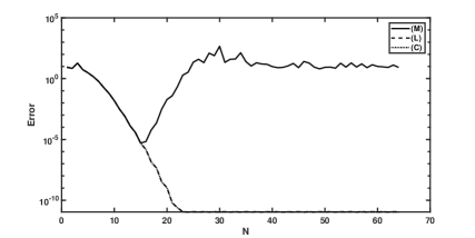
(1)

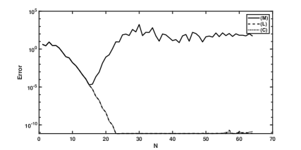
(2)

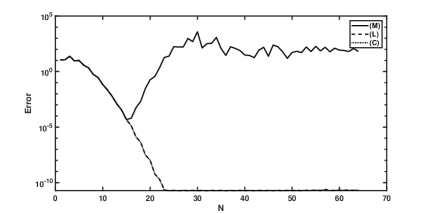
(3)

Figure 4: Error of the approximate solution in Experiment 4. The abbreviations (M) for the monomial basis, (L) for the Legendre basis, and (C) for the Chebyshev basis are used. The error is measured in the norms of (1) $L^{2}((0,1),\mathbb{R}^{m})$, (2) $L^{\infty}((0,1),\mathbb{R}^{m})$, and (3) $H_{D}^{1}((0,1),\mathbb{R}^{m})$.

In this experiment we intend to clarify the differences between different representations of the Runge-Kutta basis. The interpolation points have been fixed to be the Gauss-Legendre nodes. The Runge-Kutta basis has been represented with respect to the monomial, Legendre, and Chebyshev bases. The results are shown in Figure 4. This test indicates that the monomial basis is much less robust than the others for $N>15$ while the other representations behave very similar. ∎

 

Experiment 5

Robustness of the Runga-Kutta basis with respect to the node sequence

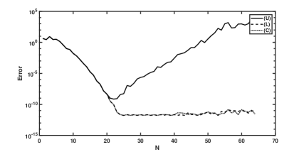
(2)

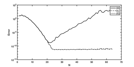
(3)

Figure 5: Error of the approximate solution in Experiment 5. The abbreviations (U) for uniform nodes, (L) for the Gauss-Legendre nodes, and (C) for the Chebyshev nodes are used. The error is measured in the norms of (1) $L^{2}((0,1),\mathbb{R}^{m})$, (2) $L^{\infty}((0,1),\mathbb{R}^{m})$, and (3) $H_{D}^{1}((0,1),\mathbb{R}^{m})$.

In this experiment we are interested in understanding the influence of the interpolation nodes. For that, we compared the uniform nodes sequence to the Gauss-Legendre and Chebyshev nodes. The uniform nodes are given by $\rho_{i}=(i-\frac{1}{2})/N$. In accordance with the results of the previous experiment, the representation of the Runge-Kutta basis in Legendre polynomials has been chosen. The results are shown in Figure 5. Not unexpectedly, uniform nodes are inferior to the other choices at least for $N>20$. However, there is no real difference between Gauss-Legendre and Chebyshev nodes. ∎

 

Experiment 6

Robustness of different polynomial representations

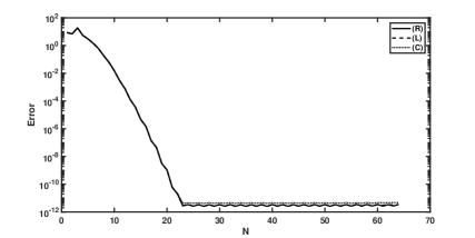
(1)

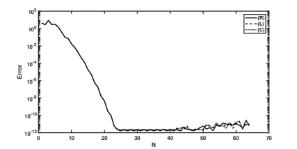
(2)

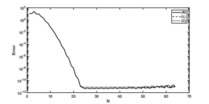
(3)

Figure 6: Error of the approximate solution in Experiment 6. The abbreviations (R) for the Runge-Kutta basis in Legendre representation, (L) for the Legendre basis, and (C) for the Chebyshev basis are used. The error is measured in the norms of (1) $L^{2}((0,1),\mathbb{R}^{m})$, (2) $L^{\infty}((0,1),\mathbb{R}^{m})$, and (3) $H_{D}^{1}((0,1),\mathbb{R}^{m})$.

In this experiment we intend to compare the robustness of different bases. Therefore, we have chosen the Runge-Kutta basis with Gauss-Legendre interpolation nodes, the Legendre polynomials, and the Chebyshev polynomials. The results are shown in Figure 6. All representations show similar behavior.  

As a conclusion, we can see that the results of the Experiments 1-3 and 4-6 are largely consistent.

Global behavior of the basis representations

We are interested in understandig the global error, which corresponds to error propagation in the case of initial value problems. In order to understand the error propagation properties we will investigate the accuracy of the computed solution with respect to an increasing number of subintervals $n$. This motivates to use a rather low order $N$ of polynomials. In the previous section we observed that there is no difference in the local properties between different basis representations for low degrees $N$ of the ansatz polynomials.

In the following experiments, the functionals used are $\Phi_{\pi,M}^{R}$ and $\Phi_{\pi,M}^{C}$. The number of collocation nodes is again $M=N+1$. The basis functions are the shifted Legendre polynomials.

The discrete problem for $n>1$ is an equality constraint linear least-squares problem. The equality constraints consists just of the continuity requirements for the differentiated components of the elements in $X_{\pi}$. The problem is solved by a direct solution method as described in Section 5. In short, the equality constraints are eliminated by a sparse QR-decomposition with column pivoting as implemented in the code SPQR SPQR . The resulting least-squares problem has then been solved by the same code.

Experiment 7

Influence of selection of collocation nodes, approximation degree $N$, and number $n$ of subintervals

In this experiment, we use Example 3 and vary the choice of collocation nodes as well as the degree $N$ of the polynomial basis and the number $n$ of subintervals. We compare Gauss-Legendre, Radau IIA and Lobatto collocation nodes. Since this example is a pure initial value problem, the use of the Radau IIA collocation nodes is especially justified. The results using $\Phi_{\pi,M}^{R}$ are collected in Table  ‣ Towards a reliable implementation of least-squares collocation for higher-index differential-algebraic equations, those using $\Phi_{\pi,M}^{C}$ in Table  ‣ Towards a reliable implementation of least-squares collocation for higher-index differential-algebraic equations. We observe no real difference between the different sets of collocation points. The results seem to confirm the conjecture that, in case of smooth problems, a higher degree $N$ is preferable over a larger $n$ or, equivalently, a smaller stepsize $h$. In addition, for the highest degree polynomials ($N=20$), the use of $\Phi_{\pi,M}^{C}$ seems to produce more accurate results than that of $\Phi_{\pi,M}^{R}$. ∎

5 The discrete least-squares problem

Once the basis has been chosen and the collocation conditions are selected, the discrete problems (18), (17), and (16) for a linear boundary value problem (1) - (2) lead to a constraint linear least-squares problem

$$\varphi(c)=\|\mathcal{A}c-r\|_{\mathbb{R}^{nmM+l}}^{2}\rightarrow\min!$$ (31)

under the constraint

$$\mathcal{C}c=0.$$ (32)

The equality constraints consists of the $k(n-1)$ continuity conditions for the approximation of the differential constraints while the functional $\varphi(c)$ represent a reformulation of the functionals (18), (17), and (16), respectively. Here, $c\in\mathbb{R}^{n(mN+k)}$ is the vector of coefficients of the basis functions for $X_{\pi}$ disregarding the continuity conditions. Furthermore, it holds $r\in\mathbb{R}^{nM}$, $\mathcal{A}\in\mathbb{R}^{(nM+l)\times n(mN+k)}$, and $\mathcal{C}\in\mathbb{R}^{(n-1)k\times n(mN+k)}$. The matrices $\mathcal{A}$ and $\mathcal{C}$ are very sparse. For details about their structure we refer to Appendix A.3.

5.1 Approaches to solve the constraint optimization problem (31)-(32)

A number of approaches to solve the constraint optimization problem (31)-(32) have been tested.

1. Direct method. The solution manifold of (32) forms a subspace which can be characterized by

   $$\mathcal{C}c=0\text{ if and only if }c=\tilde{\mathcal{C}}z\text{ for some }z\in\mathbb{R}^{nmN+k-l}.$$

   Here, $\tilde{\mathcal{C}}\in\mathbb{R}^{n(mN+k)\times(nmN+k-l)}$ has orthonormal columns. With this representation, the constrained minimization problem can be reduced to the uncontrained one

   $$\tilde{\varphi}(z)=\|\mathcal{A}\tilde{\mathcal{C}}z-r\|_{\mathbb{R}^{W}}^{2}\rightarrow\min!$$

   The implemented algorithm is that of BjorckGolub67 , see also (Bjorck96, , Section 5.1.2) which is sometimes called the direct elimination method.

2. Weighting of the constraints. In this approach, a sufficiently large parameter $\omega>0$ is chosen and the problem (31) - (32) is replaced by the free minimization problem

   $$\varphi_{\omega}(c)=\|\mathcal{A}c-r\|_{\mathbb{R}^{W}}^{2}+\omega\|\mathcal{C}c\|\rightarrow\min!$$

   It is known that the minimizer $c_{\omega}$ of $\varphi_{\omega}$ converges towards the solution of (31) - (32) for $\omega\rightarrow\infty$ (cf. (GovLo89, , Section 12.1.5)). Two different orderings of the equations have been implemented. One is

   $$\mathcal{G}=\left[\begin{array}[]{c}\omega\mathcal{C}\\ \mathcal{A}\end{array}\right],\quad\bar{r}=\left[\begin{array}[]{c}0\\ r\end{array}\right]$$

   while the other uses a block-bidiagonal structure as it is common for collocation methods for ODEs, cf BaderAscher . It is known that the order of the equations in the weighting method may have a large impact on the accuracy of the solutions vLoan85 . In our test examples, however, we did not observe a difference in the behavior of both orderings.

3. The direct solution method by eliminating the constraints has often the deficiency of generating a lot of fill-in in the intermediate matrices. An approach to overcome this situation has been proposed in vLoan85 . The solutions of the weighting approach are iteratively enhanced by a defect correction process. This method is implemented in the form presented in Barlow92 ; BarlowVemu92 . This form is called the deferred correction procedure for constrained leaset-squares problems by the authors. As a stopping criterion, the estimate (i) in (BarlowVemu92, , p. 254) has been implemented. Additionally, a bound for the maximal numer of iterations can be provided. Under reasonable conditions, at most 2 iterations should be sufficient for obtaining maximal (with respect to the sensitivity of the problem) accuracy for the discrete solution.

The results of the weighting method depend substantially on the choice of the parameter $\omega$. In order to have an accurate approximation of the exact solution $c_{\ast}$ of the problem (31)-(32), a large value of $\omega$ should be used (in the absence of rounding errors). However, if $\omega$ becomes too large, the algorithm may lack numerical stability. A discussion of this topic has been given in vLoan85 . In particular, it turns out that the algorithm used for the QR decomposition and the pivoting strategies have a strong influence on the success of this method. In our implementation, we use the sparse QR implementation of SPQR . On the other hand, an accuracy of the solution being much lower than the approximation error of $x_{\pi}$ is not necessary. Therefore, a number of experiments have been done in order to obtain some insight into what reasonable choices might be.

Experiment 8

Influence of the choice of the weighting parameter $\omega$

We use Example 3. Two sets of parameters are selected: (i) $N=5$, $n=160$ and (ii) $N=20$, $n=20$. The choice (i) corresponds to low degree polynomials with a corresponding large number of subintervals while (ii) uses higher degree polynomials with a corresponding small number of subintervals. Both cases have been selected according to Table  ‣ Towards a reliable implementation of least-squares collocation for higher-index differential-algebraic equations in such a way that a high accuracy can be obtained while at the same time having only a small influence of the problem conditioning. The other parameters chosen in this experiment are: $M=N+1$, Gauss-Legendre collocation nodes and Legendre polynomials as basis functions. The error in dependence of $\omega$ is measured both with respect to the exact solution and with respect to a reference soltion obtained by the direct solution method. The results are provided in Tables 4–5. The results for Example 4 below are quite similar. The results indicate that an optimal $\omega$ may vary considerably depending on the problem parameters. However, the accuracy against the exact solution is rather insensitive of $\omega$. ∎

Table 4: Influence of parameter $\omega$ for the constraints in Example 3 using $N=5$ and $n=160$. The error of the solution with respect to the exact solution (A) and with respect to a discrete reference solution obtained by a direct method (B) is given in the norms of $L^{2}((0,5),\mathbb{R}^{7})$, $L^{\infty}((0,5),\mathbb{R}^{7})$ and $H_{D}^{1}((0,5),\mathbb{R}^{7})$

	(A)			(B)
$\omega$	$L^{\infty}(0,5)$	$L^{2}(0,5)$	$H_{D}^{1}(0,5)$	$L^{\infty}(0,5)$	$L^{2}(0,5)$	$H_{D}^{1}(0,5)$
1e-09	2.25e+00	4.54e+00	9.37e+00	2.25e+00	4.54e+00	8.04e+00
1e-08	2.00e+00	4.59e+00	9.04e+00	2.00e+00	4.59e+00	9.04e+00
1e-07	3.55e-01	5.83e-01	1.05e+00	3.55e-01	5.83e-01	1.05e+00
1e-06	1.06e-05	1.66e-05	2.84e-05	1.06e-05	1.66e-05	2.84e-05
1e-05	1.02e-07	1.60e-07	3.07e-07	1.02e-07	1.60e-07	2.75e-07
1e-04	2.26e-08	1.49e-08	1.41e-07	5.51e-09	6.27e-09	3.51e-08
1e-03	2.26e-08	1.53e-08	1.41e-07	5.51e-09	7.09e-09	3.54e-08
1e-02	2.15e-08	1.39e-08	1.40e-07	4.44e-09	3.36e-09	3.31e-08
1e-01	2.13e-08	1.39e-08	1.40e-07	4.28e-09	3.28e-09	3.29e-08
1e+00	2.00e-08	1.31e-08	1.31e-07	2.99e-09	2.99e-09	2.29e-08
1e+01	1.73e-08	1.12e-08	1.13e-07	1.27e-10	7.51e-11	7.53e-10
1e+02	1.73e-08	1.12e-08	1.12e-07	3.64e-10	3.84e-11	3.85e-10
1e+03	1.73e-08	1.12e-08	1.12e-07	2.36e-09	3.05e-10	3.06e-09
1e+04	2.15e-08	1.15e-08	1.16e-07	1.82e-08	2.91e-09	2.92e-08
1e+05	1.18e-07	3.27e-08	3.28e-07	1.26e-07	3.18e-08	3.20e-07
1e+06	6.69e-06	5.08e-07	5.08e-06	6.68e-06	5.08e-07	5.09e-06
1e+07	6.28e-05	5.09e-06	5.09e-05	6.28e-05	5.09e-06	5.09e-05
1e+08	9.94e-05	2.82e-05	2.83e-04	9.94e-05	2.82e-05	2.83e-04
1e+09	3.33e+01	7.87e+00	7.91e+01	3.33e+01	7.87e+00	7.91e+01
1e+10	8.61e+01	5.91e+01	5.93e+02	8.61e+01	5.91e+01	5.93e+02

Table 5: Influence of parameter $\omega$ for the constraints in Example 3 using $N=20$ and $n=20$. The error of the solution with respect to the exact solution (A) and with respect to a discrete reference solution obtained by a direct method (B) is given in the norms of $L^{2}((0,5),\mathbb{R}^{7})$, $L^{\infty}((0,5),\mathbb{R}^{7})$ and $H_{D}^{1}((0,5),\mathbb{R}^{7})$

	(A)			(B)
$\omega$	$L^{\infty}(0,5)$	$L^{2}(0,5)$	$H_{D}^{1}(0,5)$	$L^{\infty}(0,5)$	$L^{2}(0,5)$	$H_{D}^{1}(0,5)$
1e-09	2.44e+00	4.91e+00	7.59e+00	2.44e+00	4.91e+00	7.59e+00
1e-08	4.40e-02	7.51e-02	1.31e-01	4.40e-02	7.51e-02	1.31e-01
1e-07	6.38e-08	9.91e-08	1.85e-07	6.38e-08	9.91e-08	1.85e-07
1e-06	1.35e-08	2.38e-08	3.80e-08	1.35e-08	2.38e-08	3.80e-08
1e-05	2.76e-09	3.68e-09	6.77e-09	2.76e-09	3.68e-09	6.77e-09
1e-04	1.86e-10	2.77e-10	5.11e-10	1.86e-10	2.77e-10	5.13e-10
1e-03	5.12e-11	1.59e-11	5.68e-11	4.59e-11	1.60e-11	6.23e-11
1e-02	2.49e-11	4.53e-12	4.29e-11	4.25e-11	5.62e-12	5.43e-11
1e-01	3.63e-11	4.57e-12	4.59e-11	5.97e-11	6.32e-12	6.35e-11
1e+00	6.01e-11	5.37e-12	5.40e-11	8.58e-11	7.61e-12	7.64e-11
1e+01	1.51e-10	1.64e-11	1.64e-10	1.53e-10	1.60e-11	1.61e-10
1e+02	4.67e-10	4.35e-11	4.37e-10	4.39e-10	4.14e-11	4.16e-10
1e+03	1.29e-08	8.11e-10	8.15e-09	1.29e-08	8.13e-10	8.17e-09
1e+04	1.50e-07	8.22e-09	8.26e-08	1.50e-07	8.22e-09	8.26e-08
1e+05	6.26e-07	4.26e-08	4.28e-07	6.26e-07	4.26e-08	4.28e-07
1e+06	1.10e-05	7.53e-07	7.57e-06	1.10e-05	7.53e-07	7.57e-06
1e+07	3.43e-05	3.17e-06	3.19e-05	3.43e-05	3.17e-06	3.19e-05
1e+08	1.85e-04	1.22e-05	1.23e-04	1.85e-04	1.22e-05	1.23e-04
1e+09	1.77e-05	3.69e-06	3.22e-05	1.77e-05	3.69e-06	3.22e-05
1e+10	6.74e+00	2.38e+00	1.47e+01	6.74e+00	2.38e+00	1.47e+01

The following example is a boundary value problem incontrast to Example 3 which is an intial value problem.

Example 4

On the interval $[0,1]$, consider the DAE

$$\left[\begin{array}[]{cccccc}1&0&0&0&0&0\\ 0&1&0&0&0&0\\ 0&0&0&0&0&0\\ 0&0&1&0&0&0\\ 0&0&0&1&0&0\\ 0&0&0&0&1&0\end{array}\right]\frac{d}{dt}\left[\begin{array}[]{c}x_{1}\\ x_{2}\\ y_{1}\\ y_{2}\\ y_{3}\\ y_{4}\end{array}\right]+\left[\begin{array}[]{cccccc}0&-\lambda&0&0&0&0\\ -\lambda&0&0&0&0&0\\ -1&0&1&0&0&0\\ 0&0&0&1&0&0\\ 0&0&0&0&1&0\\ 0&0&0&0&0&1\end{array}\right]\left[\begin{array}[]{c}x_{1}\\ x_{2}\\ y_{1}\\ y_{2}\\ y_{3}\\ y_{4}\end{array}\right]=\left[\begin{array}[]{c}0\\ 0\\ 0\\ 0\\ 0\\ 0\end{array}\right],\quad\lambda>0,$$

subject to the boundary conditions

$$x_{1}(0)=x_{1}(1)=1.$$

This DAE can be brought into the proper form (1) by setting

$$A=\left[\begin{array}[]{ccccc}1&0&0&0&0\\ 0&1&0&0&0\\ 0&0&0&0&0\\ 0&0&1&0&0\\ 0&0&0&1&0\\ 0&0&0&0&1\end{array}\right],\quad D=\left[\begin{array}[]{cccccc}1&0&0&0&0&0\\ 0&1&0&0&0&0\\ 0&0&1&0&0&0\\ 0&0&0&1&0&0\\ 0&0&0&0&1&0\end{array}\right],\quad B=\left[\begin{array}[]{cccccc}0&-\lambda&0&0&0&0\\ -\lambda&0&0&0&0&0\\ -1&0&1&0&0&0\\ 0&0&0&1&0&0\\ 0&0&0&0&1&0\\ 0&0&0&0&0&1\end{array}\right].$$

This DAE has the tractability index $\mu=4$ and dynamical degree of freedom $l=2$. The solution reads

$$x_{\ast,1}(t) =\frac{e^{-\lambda t}(e^{\lambda}+e^{2\lambda t})}{1+e^{\lambda}}$$

$$x_{\ast,2}(t) =\frac{e^{-\lambda t}(-e^{\lambda}+e^{2\lambda t})}{1+e^{\lambda}}$$

$$y_{\ast,1}(t) =\frac{e^{-\lambda t}(e^{\lambda}+e^{2\lambda t})}{1+e^{\lambda}}$$

$$y_{\ast,2}(t) =\lambda\frac{e^{-\lambda t}(-e^{\lambda}+e^{2\lambda t})}{1+e^{\lambda}}$$

$$y_{\ast,3}(t) =\lambda^{2}\frac{e^{-\lambda t}(e^{\lambda}+e^{2\lambda t})}{1+e^{\lambda}}$$

$$y_{\ast,4}(t) =\lambda^{3}\frac{e^{-\lambda t}(-e^{\lambda}+e^{2\lambda t})}{1+e^{\lambda}}$$

∎

The iterative solver using defect corrections may overcome the difficulties connected with a suitable choice of the parameter $\omega$ in the weighting method. According to Experiment 10, we would expect the optimal $\omega$ to be in the order of magnitude $10^{-3}\ldots 10^{+2}$ with an optimum around $10^{-2}$. This is in contrast to the recommendations given in BarlowVemu92 where a choice of $\omega\approx\varepsilon_{\text{mach}}^{-1/3}$ is recommended for the deferred correction algorithm. We test the performance of the deferred correction solver in the next experiment. Here, the tolerance in the convergence check is set to $10^{-15}$. The iterations are considered not to converge if the convergence check has failed after two iterations.

Experiment 9

We check the performance of the deferred correction solver in dependence of the weight parameter $\omega$. Both Examples 3 and 4 are used. The results are presented in Tables 6 – 9. The results indicate that a larger value for $\omega$ seems to be preferable. ∎

Table 6: Influence of the parameter $\omega$ on the accuracy of th discrete solution for Example 3 using $N=5$ and $n=160$. The error of the solution with respect to the exact solution (A) and with respect to a discrete reference solution obtained by a direct method (B) is given in the norms of $L^{2}((0,5),\mathbb{R}^{7})$, $L^{\infty}((0,5),\mathbb{R}^{7})$ and $H_{D}^{1}((0,5),\mathbb{R}^{7})$. 2 iterations are applied

	(A)			(B)
$\omega$	$L^{\infty}(0,5)$	$L^{2}(0,5)$	$H_{D}^{1}(0,5)$	$L^{\infty}(0,5)$	$L^{2}(0,5)$	$H_{D}^{1}(0,5)$
0.01	2.13e-08	1.39e-08	1.40e-07	4.30e-09	3.30e-09	3.31e-08
10	1.73e-08	1.12e-08	1.12e-07	5.43e-11	1.62e-11	1.63e-10
$\varepsilon_{\text{mach}}^{-1/3}$	1.73e-08	1.12e-08	1.12e-07	5.42e-11	1.62e-11	1.63e-10

Table 7: Influence of the parameter $\omega$ on the accuracy of th discrete solution for Example 3 using $N=20$ and $n=20$. The error of the solution with respect to the exact solution (A) and with respect to a discrete reference solution obtained by a direct method (B) is given in the norms of $L^{2}((0,5),\mathbb{R}^{7})$, $L^{\infty}((0,5),\mathbb{R}^{7})$ and $H_{D}^{1}((0,5),\mathbb{R}^{7})$. 2 iterations are applied

	(A)			(B)
$\omega$	$L^{\infty}(0,5)$	$L^{2}(0,5)$	$H_{D}^{1}(0,5)$	$L^{\infty}(0,5)$	$L^{2}(0,5)$	$H_{D}^{1}(0,5)$
0.01	2.20e-11	3.35e-12	3.37e-11	6.25e-11	6.67e-12	6.70e-11
10	1.79e-11	1.98e-12	1.99e-11	6.26e-11	6.91e-12	6.95e-11
$\varepsilon_{\text{mach}}^{-1/3}$	1.11e-11	1.71e-12	1.72e-11	6.26e-11	6.94e-12	6.97e-11

Table 8: Influence of the parameter $\omega$ on the accuracy of the discrete solution for Example 4 using $N=20$ and $n=5$. The error of the solution with respect to the exact solution (A) and with respect to a discrete reference solution obtained by a direct method (B) is given in the norms of $L^{2}((0,5),\mathbb{R}^{6})$, $L^{\infty}((0,5),\mathbb{R}^{6})$ and $H_{D}^{1}((0,5),\mathbb{R}^{6})$. 2 iterations are applied

	(A)			(B)
$\omega$	$L^{\infty}(0,5)$	$L^{2}(0,5)$	$H_{D}^{1}(0,5)$	$L^{\infty}(0,5)$	$L^{2}(0,5)$	$H_{D}^{1}(0,5)$
0.01	8.25e-08	6.17e-09	8.72e-09	2.52e-06	1.55e-07	2.20e-07
10	2.73e-07	1.41e-08	2.00e-08	2.63e-06	1.61e-07	2.27e-07
$\varepsilon_{\text{mach}}^{-1/3}$	3.84e-09	3.61e-10	5.11e-10	2.45e-06	1.56e-07	2.20e-07

Table 9: Influence of the parameter $\omega$ on the accuracy of th discrete solution for Example 4 using $N=5$ and $n=20$. The error of the solution with respect to the exact solution (A) and with respect to a discrete reference solution obtained by a direct method (B) is given in the norms of $L^{2}((0,5),\mathbb{R}^{6})$, $L^{\infty}((0,5),\mathbb{R}^{6})$ and $H_{D}^{1}((0,5),\mathbb{R}^{6})$. 2 iterations are applied

	(A)			(B)
$\omega$	$L^{\infty}(0,5)$	$L^{2}(0,5)$	$H_{D}^{1}(0,5)$	$L^{\infty}(0,5)$	$L^{2}(0,5)$	$H_{D}^{1}(0,5)$
0.01	1.41e-06	4.59e-07	6.49e-07	3.75e-08	4.23e-09	5.98e-09
10	1.39e-06	4.59e-07	6.49e-07	1.42e-08	2.63e-09	3.71e-09
$\varepsilon_{\text{mach}}^{-1/3}$	1.39e-06	4.59e-07	6.49e-07	1.71e-08	2.83e-09	4.00e-09

5.2 Performance of the linear solvers

In this section, we intend to provide some insight into the behavior of the linear solvers. This concerns both the accuracy as well as the computational resources (computation time, memory consumption). All these data are highly implementation dependent. Also the hardware architecture plays an important role.

The linear solvers have been implemented using the standard strategy of subdividing them into a factorization step and a solve step. The price to pay is a larger memory consumption. However, their use in the context of, e.g., a modified Newton method may decrease the computation time considerably.

The tests have benn run on a Linux laptop Dell Latitude E5550. While the program is a pure sequential one, the MKL library may use shared memory parallel versions of their BLAS and LAPACK routines. The CPU of the machine is an Intel(R) Core(TM) i7-5600U CPU @ 2.60GHz providing two cores, each of them capable of hyperthreading. For the test runs, cpu throttling has been disabled such that all cores ran at roughly 3.2 GHz.

The parameter for the weighting solver is $\omega=1$ while the corresponding parameter for the deferred correction solver is $\omega=\epsilon_{\textrm{mach}}^{-1/3}\approx 1.65\times 10^{5}$. These parameters have been chosen since they seem to be best suited for the examples. The test cases (combination of $N$ and $n$) have been selected by choosing the best combinations in Tables  ‣ Towards a reliable implementation of least-squares collocation for higher-index differential-algebraic equations and ‣ Towards a reliable implementation of least-squares collocation for higher-index differential-algebraic equations, respectively.

Experiment 10

First, we consider Example 3. For all values of $N$, $M=N+1$ Gauss-Legendre nodes have been used. The characteristics of the test cases using Legendre basis functions are provided in Table 10. For the special properties of the Legendre polynomials, the matrix $\mathcal{C}$ representing the constraints is extremly sparse featuring only three nonzero elements per row. The computational results are shown in Table 11. In the next computations, the Chebyshev basis has been used which leads to a slightly more occupied matrix $\mathcal{C}$. The results are provided in Tables 12 and 13.

Table 10: Case characteristics for Experiment 10 using the Legendre basis. The number of nonzero elements in the matrices $\mathcal{A}$ and $\mathcal{C}$ are provided as reported by the functions of the Eigen library. The columns denote: the number of rows of $\mathcal{A}$ (dimA), the number of rows of $\mathcal{C}$ (dimC), the number of unknowns (nun), the number of nonzero elements of $\mathcal{C}$ (nnzC), the number of nonzero elements of $\mathcal{A}$ (nnzA) for the functional $\Phi^{R}_{\pi,M}$ and $\Phi^{C}_{\pi,M}$, respectively

							$\Phi_{\pi,M}^{R}$	$\Phi_{\pi,M}^{C}$
case	$N$	$n$	dimA	dimC	nun	nnzC	nnzA	nnzA
1	3	320	8964	1914	8640	5742	101124	101124
2	5	80	3364	474	3280	1422	58964	59044
3	10	5	389	24	380	72	12749	12334
4	20	5	739	24	730	72	47509	46534

Table 11: Computing times, permanent workspace needed, and error for the cases described in Table 10. The computing times are provided in milliseconds. They are the average of 100 runs of each case. The error is measured in the norm of $H^{1}_{D}((0,5),\mathbb{R}^{7})$. The column headings denote: The upper bound on the number of nonzero elements of the $QR$-factors as reported by SPQR (nWork), the time for the matrix assembly (tass), the time for the factorization (afact), and the time for the solution (tslv) for both functionals $\Phi^{R}_{\pi,M}$ and $\Phi^{C}_{\pi,M}$

		$\Phi_{\pi,M}^{R}$					$\Phi_{\pi,M}^{C}$
case	solver	nWork	tass	tfact	tslv	error	nWork	tass	tfact	tslv	error
1	direct	221829	12	156	4	6.74e-04	221829	12	158	4	6.44e-04
	weighted	309438	13	17	6	1.15e-03	309438	13	19	6	6.93e-04
	deferred	309438	14	18	16	6.74e-04	309438	13	18	17	6.44e-04
2	direct	115932	12	50	4	9.02e-07	116168	5	25	2	8.50e-07
	weighted	155334	14	17	6	1.05e-06	155370	6	8	3	8.95e-07
	deferred	155334	14	16	14	9.02e-07	155370	6	8	7	8.50e-07
3	direct	24233	2	4	1	8.80e-08	24967	1	2	0	6.59e-08
	weighted	26810	2	3	1	9.62e-08	27028	1	1	0	8.00e-08
	deferred	26810	2	3	2	8.80e-08	27028	1	1	1	6.59e-08
4	direct	90277	9	2	2	4.47e-12	90052	1	1	2	5.17e-12
	weighted	96544	11	10	3	7.44e-12	97857	9	11	3	5.28e-12
	deferred	96544	11	10	6	2.17e-12	97857	9	10	5	2.08e-12

Table 12: Case characteristics for Experiment 10 using the Chebyshev basis. The number of nonzero elements in the matrices $\mathcal{A}$ and $\mathcal{C}$ are provided as reported by the functions of the Eigen library. The columns denote: the number of rows of $\mathcal{A}$ (dimA), the number of rows of $\mathcal{C}$ (dimC), the number of unknowns (nun), the number of nonzero elements of $\mathcal{C}$ (nnzC), the number of nonzero elements of $\mathcal{A}$ (nnzA) for the functional $\Phi^{R}_{\pi,M}$ and $\Phi^{C}_{\pi,M}$, respectively

							$\Phi_{\pi,M}^{R}$	$\Phi_{\pi,M}^{C}$
case	$N$	$n$	dimA	dimC	nun	nnzC	nnzA	nnzA
1	3	320	8964	1914	8640	7656	101128	101124
2	5	80	3364	474	3280	3318	58851	59056
3	10	5	389	24	380	360	12846	12626
4	20	5	739	24	730	720	47581	47191

Table 13: Computing times, permanent workspace needed, and error for the cases described in Table 12. The computing times are provided in milliseconds. They are the average of 100 runs of each case. The error is measured in the norm of $H^{1}_{D}((0,5),\mathbb{R}^{7})$. The column headings denote: The upper bound on the number of nonzero elements of the $QR$-factors as reported by SPQR (nWork), the time for the matrix assembly (tass), the time for the factorization (afact), and the time for the solution (tslv) for both functionals $\Phi^{R}_{\pi,M}$ and $\Phi^{C}_{\pi,M}$

		$\Phi_{\pi,M}^{R}$					$\Phi_{\pi,M}^{C}$
case	solver	nWork	tass	tfact	tslv	error	nWork	tass	tfact	tslv	error
1	direct	334564	12	161	6	6.74e-04	329266	15	163	6	6.44e-04
	weighted	367514	14	21	8	1.15e-03	358591	15	23	8	6.93e-04
	deferred	367514	13	21	21	6.74e-04	358591	15	22	22	6.44e-04
2	direct	231988	12	61	7	9.02e-07	231962	5	30	4	8.50e-07
	weighted	204243	14	23	8	1.05e-06	201128	6	11	4	8.95e-07
	deferred	204243	14	23	21	9.02e-07	201128	6	11	10	8.50e-07
3	direct	51343	2	7	1	8.80e-08	51565	2	7	1	6.59e-08
	weighted	60861	2	5	1	9.62e-08	61376	2	5	1	8.00e-08
	deferred	60861	3	5	3	8.80e-08	61376	2	5	3	6.59e-08
4	direct	208910	9	3	4	5.78e-12	230195	7	28	5	5.17e-12
	weighted	164558	11	15	4	5.37e-12	167836	9	15	3	4.75e-12
	deferred	164558	11	15	8	2.71e-12	167836	10	15	8	2.23e-12

The previous example is an initial value problem. This structure may have consequences on the performance of the linear solvers. Therefore, in the next experiment, we consider a boundary value problem.

Experiment 11

We repeat Experiment 10 with Example 4. The problem characteristics and computational results are provided in Tables 14 – 17. It should be noted that the deferred correction solver returned normally (tolerance as before $10^{-15}$) after at most two iterations in all cases. However, in some cases, the results are completely off. This happens, for example, in Tables 15 and 17, cases 1 and 2, for $\Phi_{\pi,M}^{C}$.

Table 14: Case characteristics for Experiment 11 using the Legendre basis. The number of nonzero elements in the matrices $\mathcal{A}$ and $\mathcal{C}$ are provided as reported by the functions of the Eigen library. The columns denote: the number of rows of $\mathcal{A}$ (dimA), the number of rows of $\mathcal{C}$ (dimC), the number of unknowns (nun), the number of nonzero elements of $\mathcal{C}$ (nnzC), the number of nonzero elements of $\mathcal{A}$ (nnzA) for the functional $\Phi^{R}_{\pi,M}$ and $\Phi^{C}_{\pi,M}$, respectively

							$\Phi_{\pi,M}^{R}$	$\Phi_{\pi,M}^{C}$
case	$N$	$n$	dimA	dimC	nun	nnzC	nnzA	nnzA
1	4	320	9602	1595	9280	4785	86403	80643
2	5	160	5762	795	5600	1422	63363	63363
3	10	5	332	20	325	60	6933	6663
4	20	5	632	20	625	60	25793	25263

Table 15: Computing times, permanent workspace needed, and error for the cases described in Table 14. The computing times are provided in milliseconds. They are the average of 100 runs of each case. The error is measured in the norm of $H^{1}_{D}((0,1),\mathbb{R}^{6})$. The column headings denote: The upper bound on the number of nonzero elements of the $QR$-factors as reported by SPQR (nWork), the time for the matrix assembly (tass), the time for the factorization (afact), and the time for the solution (tslv) for both functionals $\Phi^{R}_{\pi,M}$ and $\Phi^{C}_{\pi,M}$

		$\Phi_{\pi,M}^{R}$					$\Phi_{\pi,M}^{C}$
case	solver	nWork	tass	tfact	tslv	error	nWork	tass	tfact	tslv	error
1	direct	437085	14	164	8	1.58e-04	397127	13	158	7	1.24e-04
	weighted	235746	14	16	5	8.22e-05	341713	7	22	7	2.07e-05
	deferred	235746	14	16	13	5.53e-02	341713	14	21	25	9.09e+02
2	direct	348742	17	124	12	2.58e-05	348742	15	123	12	1.57e-05
	weighted	153062	9	9	3	9.29e-07	153062	9	9	3	7.75e-06
	deferred	153062	10	9	8	1.38e-01	153062	9	10	10	1.47e-01
3	direct	11617	1	3	0	8.04e-10	12155	1	2	0	1.06e-09
	weighted	12400	2	2	1	1.26e-09	12141	1	1	0	5.52e-09
	deferred	12400	2	2	1	4.18e-11	12141	1	1	1	5.08e-09
4	direct	46847	6	9	1	7.24e-08	46883	2	4	7	3.54e-07
	weighted	42947	7	6	2	1.42e-07	42859	3	3	1	1.71e-07
	deferred	42947	6	6	4	5.27e-09	42859	3	3	2	1.51e-07

Table 16: Case characteristics for Experiment 11 using the Chebyshev basis. The number of nonzero elements in the matrices $\mathcal{A}$ and $\mathcal{C}$ are provided as reported by the functions of the Eigen library. The columns denote: the number of rows of $\mathcal{A}$ (dimA), the number of rows of $\mathcal{C}$ (dimC), the number of unknowns (nun), the number of nonzero elements of $\mathcal{C}$ (nnzC), the number of nonzero elements of $\mathcal{A}$ (nnzA) for the functional $\Phi^{R}_{\pi,M}$ and $\Phi^{C}_{\pi,M}$, respectively

							$\Phi_{\pi,M}^{R}$	$\Phi_{\pi,M}^{C}$
case	$N$	$n$	dimA	dimC	nun	nnzC	nnzA	nnzA
1	4	320	9602	1595	9280	7656	86406	82566
2	5	160	5762	795	5600	5565	63367	63367
3	10	5	332	20	325	300	6945	6795
4	20	5	632	20	325	600	25830	25560

Table 17: Computing times, permanent workspace needed, and error for the cases described in Table 16. The computing times are provided in milliseconds. They are the average of 100 runs of each case. The error is measured in the norm of $H^{1}_{D}((0,1),\mathbb{R}^{6})$. The column headings denote: The upper bound on the number of nonzero elements of the $QR$-factors as reported by SPQR (nWork), the time for the matrix assembly (tass), the time for the factorization (afact), and the time for the solution (tslv) for both functionals $\Phi^{R}_{\pi,M}$ and $\Phi^{C}_{\pi,M}$

		$\Phi_{\pi,M}^{R}$					$\Phi_{\pi,M}^{C}$
case	solver	nWork	tass	tfact	tslv	error	nWork	tass	tfact	tslv	error
1	direct	796757	27	360	28	6.77e-05	807507	26	363	29	1.77e-04
	weighted	502962	16	28	11	1.90e-06	471966	16	29	11	1.11e-05
	deferred	502962	15	28	27	2.33e-07	471966	15	29	35	1.19e+02
2	direct	513054	17	143	16	3.59e-05	513054	15	143	17	2.37e-05
	weighted	347439	10	19	7	8.73e-07	347439	9	19	7	4.71e-06
	deferred	Solver failed					347439	9	20	25	5.07e+02
3	direct	29347	2	4	1	2.69e-09	30843	1	3	1	1.40e-09
	weighted	25392	2	3	1	5.10e-10	26984	1	1	0	8.52e-10
	deferred	25392	2	2	2	4.41e-11	26984	1	1	1	1.22e-09
4	direct	122665	6	16	3	6.70e-08	148882	5	18	4	6.68e-07
	weighted	109429	7	10	3	5.22e-08	109345	6	10	3	5.43e-08
	deferred	109429	7	11	7	6.09e-11	109345	6	11	7	2.62e-09

It should be noted that a considerable amount of memory for the QR-factorizations is consumed by the internal representation of the Q-factor in SPQR. This can be avoided if the factorization and solution steps are intervowen.

5.3 Sensitivity of boundary condition weighting

As already known for boundary value problems for ODEs and index-1 DAEs, a special problem is the scaling of the boundary condition, and hence, here the inclusion of the boundary conditions (2). Their scaling is independent of the scaling of the DAE (1). Therefore, it seems to be reasonable to provide an additional possibility for the scaling of the boundary conditions. We decided to enable this by introducing an additional parameter $\alpha$ to be chosen by the user. So, $\Phi$ from (8) is replaced by the functional

$$\tilde{\Phi}(x)=\int_{a}^{b}|A(t)(Dx)^{\prime}(t)+B(t)x(t)-q(t)|^{2}{\rm dt}+\alpha|G_{a}x(a)+G_{b}x(b)-d|^{2}.$$

Analogously, the discretized versions $\Phi_{\pi,M}^{R}$, $\Phi_{\pi,M}^{I}$ and $\Phi_{\pi,M}^{C}$ are replaced by their counterparts $\tilde{\Phi}_{\pi,M}^{R}$, $\tilde{\Phi}_{\pi,M}^{I}$ and $\tilde{\Phi}_{\pi,M}^{C}$ with weighted boundary conditions. The convergence theorems will hold true for these modifications of the functional, too.

Experiment 12

Influence of $\alpha$ on the accuracy

We use the example and settings of Experiment 8. The results are provided in Table 18. ∎

Table 18: Influence of weight parameter $\alpha$ for the boundary conditions in Example 3. The error of the solution is given in the norms of $L^{2}((0,5),\mathbb{R}^{7})$, $L^{\infty}((0,5),\mathbb{R}^{7})$ and $H_{D}^{1}((0,5),\mathbb{R}^{7})$

	$N=5$, $n=160$			$N=20$, $n=20$
$\alpha$	$L^{\infty}(0,5)$	$L^{2}(0,5)$	$H_{D}^{1}(0,5)$	$L^{\infty}(0,5)$	$L^{2}(0,5)$	$H_{D}^{1}(0,5)$
1e-10	3.18e+00	7.03e+00	1.21e+01	1.60e+00	3.10e+00	5.09e+00
1e-09	9.33e-07	2.33e-06	3.84e-06	1.60e+00	3.10e+00	5.09e+00
1e-08	1.58e-07	3.52e-07	6.16e-07	1.05e-07	1.94e-07	3.54e-07
1e-07	1.27e-07	1.39e-08	3.26e-08	5.06e-09	1.10e-08	2.00e-08
1e-06	7.17e-08	2.20e-09	1.68e-08	9.60e-10	2.29e-09	4.10e-09
1e-05	9.60e-08	1.59e-09	1.58e-08	7.64e-11	2.07e-10	3.80e-10
1e-04	6.99e-08	1.59e-09	1.60e-08	5.00e-11	4.07e-11	9.26e-11
1e-03	9.83e-08	1.82e-09	1.83e-08	3.91e-11	6.41e-12	5.46e-11
1e-02	1.15e-07	2.28e-09	2.29e-08	6.37e-11	6.26e-12	6.25e-11
1e-01	6.43e-08	1.27e-09	1.27e-08	5.11e-11	6.61e-12	6.64e-1
1e+00	6.04e-08	1.13e-09	1.13e-08	6.66e-11	7.50e-12	7.54e-11
1e+01	2.15e-07	3.40e-09	3.42e-08	7.97e-11	9.85e-12	9.89e-11
1e+02	4.12e-07	5.66e-09	5.68e-08	6.78e-11	8.10e-12	8.14e-11
1e+03	4.51e-06	5.74e-08	5.76e-07	9.60e-11	9.81e-12	9.85e-11
1e+04	2.31e-05	2.93e-07	2.95e-06	2.24e-09	1.52e-10	1.52e-09
1e+05	4.68e-04	5.94e-06	5.97e-05	2.91e-08	1.35e-09	1.36e-08
1e+06	2.12e+03	5.16e+01	5.19e+02	2.34e-07	1.68e-08	1.68e-07
1e+07	6.53e+03	1.03e+02	1.04e+03	2.97e-06	1.77e-07	1.77e-06
1e+08	4.60e+02	1.78e+01	1.79e+02	4.76e-06	3.72e-07	3.73e-06
1e+09	2.05e+01	3.27e+00	3.24e+01	4.56e+01	4.90e+00	4.91e+01

Experiment 13

Influence of $\alpha$ on the accuracy

We repeat the previous experiment with Example 4. The discretization parameters are (i) $N=5$, $n=20$ and (ii) $N=20$, $n=5$. All other settings correspond to those of Experiment 12. The results are presented in Table 19. ∎

Table 19: Influence of weight parameter $\alpha$ for the boundary conditions in Example 4. The error of the solution is given in the norms of $L^{2}((0,1),\mathbb{R}^{6})$, $L^{\infty}((0,1),\mathbb{R}^{6})$ and $H_{D}^{1}((0,1),\mathbb{R}^{6})$

	$N=5$, $n=20$			$N=20$, $n=5$
$\alpha$	$L^{\infty}(0,1)$	$L^{2}(0,1)$	$H_{D}^{1}(0,1)$	$L^{\infty}(0,1)$	$L^{2}(0,1)$	$H_{D}^{1}(0,1)$
1e-10	4.21e-02	7.02e-02	9.13e-02	1.03e-06	8.55e-08	1.21e-07
1e-09	4.46e-04	7.38e-04	9.60e-04	1.00e-06	6.11e-08	8.64e-08
1e-08	4.40e-06	6.71e-06	8.80e-06	1.14e-06	6.48e-08	9.16e-08
1e-07	1.47e-06	4.87e-07	6.88e-07	9.84e-07	6.02e-08	8.51e-08
1e-06	1.39e-06	4.59e-07	6.49e-07	1.67e-06	1.10e-07	1.56e-07
1e-05	1.40e-06	4.59e-07	6.49e-07	1.19e-06	8.21e-08	1.16e-07
1e-04	1.40e-06	4.59e-07	6.49e-07	8.55e-07	6.48e-08	9.17e-08
1e-03	1.40e-06	4.59e-07	6.49e-07	1.44e-06	1.04e-07	1.47e-07
1e-02	1.40e-06	4.59e-07	6.49e-07	5.14e-07	4.77e-08	6.75e-08
1e-01	1.40e-06	4.59e-07	6.49e-07	1.69e-06	8.49e-08	1.20e-07
1e+00	1.40e-06	4.59e-07	6.49e-07	2.45e-06	1.56e-07	2.20e-07
1e+01	1.40e-06	4.59e-07	6.49e-07	1.83e-06	1.09e-07	1.54e-07
1e+02	1.40e-06	4.59e-07	6.49e-07	1.91e-05	8.14e-07	1.15e-06
1e+03	1.40e-06	4.59e-07	6.49e-07	1.40e-04	1.10e-06	1.55e-06
1e+04	1.41e-06	4.59e-07	6.49e-07	1.27e-03	5.34e-05	7.56e-05
1e+05	1.39e-06	4.59e-07	6.49e-07	3.69e-04	1.94e-05	2.75e-05
1e+06	1.63e-06	4.66e-07	6.59e-07	3.98e-04	3.42e-05	4.83e-05
1e+07	1.99e+02	5.07e+01	7.18e+01	2.11e-03	3.53e-04	4.99e-04
1e+08	1.99e+02	5.07e+01	7.18e+01	1.22e-01	2.83e-02	4.01e-02
1e+09	1.99e+02	5.07e+01	7.18e+01	4.86e-01	2.05e-01	2.90e-01

The results of Experiments 12 and 13 indicate that the final accuracy is rather insensitive to the choice of $\alpha$. It should be noted that the coefficient matrices in Examples 3 and 4 are well-scaled.

6 Final remarks and conclusions

In summary, in the present paper, we investigated questions related to an efficient and reliable realization of a least-squares collocation method. These questions are particularly important since a higher index DAE is an essentially ill-posed problem in naturally given spaces, which is why we must be prepared for highly sensitive discrete problems. In order to obtain a overall procedure that is as robust as possible, we provided criteria which led to a robust selection of the collocation points and of the basis functions, whereby the latter is also useful for the shape of the resulting discrete problem. Additionally, a number of new, more detailed, error estimates have been given that support some of the design decisions. The following particular items are worth highlighting in this context:

• The basis for the approximation space should be appropriately shifted and scaled orthogonal polynomials. We could not observe any larger differences between the behavior of Legendre and Chebyshev polynomials.

• The collocation points should be chosen to be the Gauss-Legendre, Lobatto, or Radau nodes. This leads to discrete problems whose conditioning using the discretization by interpolation ($\Phi_{\pi,M}^{R}$) is not much worse than that resembling collocation methods for ordinary differential equations ($\Phi_{\pi,M}^{C}$). A particular efficient and stable implementation is obtained if Gauss-Legendre or Radau nodes are used since, in this case, diagonal weighting ($\Phi_{\pi,M}^{I}$) coincides with the interpolation approach.

• A critical ingredient for the implementation of the method is the algorithm used for the solution of the constrained linear least-squares problems. Given the expected bad conditioning of the least-squares problem, a QR-factorization with column pivoting must lie at the heart of the algorithm. At the same time, the sparsity structure must be used as best as possible. In our tests, the direct solver seems to be the most robust one. With respect to efficiency and accuracy, the deferred correction solver is preferable. However, it failed in certain tests.

• It seems as if, for problems with a smooth solution, a higher degree $N$ of the ansatz polynomials with a low number of subintervals $n$ in the mesh is preferable over a smaller degree with a larger number of subintervals with respect to accuracy. Some first theoretical justification has been provided for this claim.

• So far, in all experiments of this and previously published papers, we did not observe any serious differences in the accuracy obtained in dependence on the choice of $M>N$ for fixed $n$. The results for $M=N+1$ are not much different from those obtained for a larger $M$.

• While superconvergence in classical collocation for ODEs and index-1 DAEs is a very favorable phenomenon, we could not find anything analogous in all our experiments.

• The simple collocation procedure using $\Phi_{\pi,M}^{C}$ performs surprisingly well. In fact, the results are, in our experiments, in par with those using $\Phi_{\pi,M}^{R}=\Phi_{\pi,M}^{I}$. However, we have no theoretical justification for this as yet.

• Our method is designed for variable grids. However, so far we have only worked with constant step size. In order to be able to adapt the grid and the polynomial degree, or even select appropriate grids, it is important to understand the structure of the error, that is, how the global error depends on local errors. This is a very important open problem, for which we have no solution yet.

In conclusion, we note that earlier implementations, among others the one from the very first paper in this matter HMTWW , which started from proven ingredients for ODE codes, are from today’s point of view and experience a rather bad version for the least-squares collocation. Nevertheless, the test results calculated with it were already very impressive. This strengthens our belief that a careful implementation of the method gives rise to a very efficient solver for higher-index DAEs.

Appendix A Some facts about classical orthogonal polynomials

In the derivations, classical orthogonal polynomials have been heavily used. For the reader’s convenience important properties are collected below.

A.1 Legendre Polynomials

The Legendre polynomials $P_{\nu}$, $\nu=0,1,\ldots$, are defined by the recurrence relation

$$P_{0}(\tau) =1,$$

$$P_{1}(\tau) =\tau,$$ (33)

$$(\nu+1)P_{\nu+1}(\tau) =(2\nu+1)\tau P_{\nu}(\tau)-\nu P_{\nu-1}(\tau),\quad\nu=1,2,\ldots.$$

Some properties of the Legendre polynomials are

1. $P_{\nu}(-1)=(-1)^{\nu}$, $P_{\nu}(1)=1,\quad\nu=0,1,\ldots$,

2. $\int_{-1}^{1}P_{0}(\tau)=2$, $\int_{-1}^{1}P_{\nu}(\tau)=0,\quad\nu=1,2,\ldots$

3. $\int_{-1}^{1}P_{\nu}(\tau)P_{\mu}(\tau)d\tau=\frac{2}{2\nu+1}\delta_{\nu\mu},\quad\nu,\nu=0,1,\ldots$, where $\delta_{\nu\mu}$ denotes the Kronecker $\delta$-symbol,

4. $P_{\nu+1}^{\prime}(\tau)-P_{\nu-1}^{\prime}(\tau)=(2\nu+1)P_{\nu}(\tau),\quad\nu=1,2,\ldots$

The latter property is useful for representing integrals,

$$\int_{-1}^{\tau}P_{\nu}(\sigma)d\sigma =\frac{1}{2\nu+1}\left(P_{\nu+1}(\tau)-P_{\nu-1}(\tau)-(-1)^{\nu+1}+(-1)^{\nu-1}\right)$$

$$=\frac{1}{2\nu+1}\left(P_{\nu+1}(\tau)-P_{\nu-1}(\tau)\right).$$ (34)

Moreover, $\int_{-1}^{\tau}P_{0}(\sigma)d\sigma=\tau+1$.

For a stable evaluation of the Legendre polynomials, we use a representation proposed in LebedevBarburin65 ,

$$P_{\nu+1}(\tau)=\frac{\nu}{\nu+1}(\tau P_{\nu}(\tau)-P_{\nu-1}(\tau))+\tau P_{\nu}(\tau).$$

In the implementation, all polynomials must be evaluated simulataneously for each given $\tau$. The evaluation of the recursions is cheap. Linear combinations of the basis function can be conveniently and stably evaluated using the Clenshaw algorithm (FoxParker68, , p. 56)Barrio02 ; Smok02 .

The shifted Legendre polynomials $\tilde{P}_{\nu}$ are given by $\tilde{P}_{\nu}(\rho)=P_{\nu}(2\rho-1)$, $\nu=0,1,\ldots$ They fulfill the orthogonality relations

$$\int_{0}^{1}\tilde{P}_{\nu}(\rho)\tilde{P}_{\mu}(\rho)d\rho=\frac{1}{2\nu+1}\delta_{\nu\mu}.$$

Moreover, we introduce the normalized shifted Legendre polynomials $\hat{P}_{\nu}$ by

$$\hat{P}_{\nu}(\rho)=(2\nu+1)^{1/2}\tilde{P}(\rho).$$

A.2 Chebyshev polynomials

The Chebyshev polynomials of the first kind $T_{\nu}$, $\nu=0,1,\ldots$, are defined by the recurrence relation

$$T_{0}(\tau) =1,$$

$$T_{1}(\tau) =\tau,$$ (35)

$$T_{\nu+1}(\tau) =2\tau T_{\nu}(\tau)-T_{\nu-1}(\tau),\quad\nu=1,2,\ldots.$$

Some properties of the Chebyshev polynomials are

1. $T_{\nu}(-1)=(-1)^{\nu},\quad T_{\nu}(1)=1,\quad\nu=0,1,\ldots$

2. $T_{\nu}(\tau)=\frac{1}{2}\left(\frac{1}{\nu+1}T_{\nu+1}^{\prime}(\tau)-\frac{1}{\nu-1}T_{\nu-1}^{\prime}(\tau)\right),\quad\nu=2,3,\ldots$

Similarly as before, we obtain the simple presentation

$$\int_{-1}^{\tau}T_{\nu}(\sigma)d\sigma=\frac{1}{2(\nu^{2}-1)}\left((\nu-1)T_{\nu+1}(\tau)-(\nu+1)T_{\nu-1}(\tau)+(-1)^{\nu-1}2\right).$$ (36)

The orthogonality property of the Chebyshev polynomials reads

$$\int_{-1}^{1}T_{\nu}(\tau)T_{\mu}(\tau)\frac{d\tau}{\sqrt{1-x^{2}}}=\begin{cases}0,&\nu\neq\mu,\\ \pi,&\nu=\mu=0,\\ \frac{\pi}{2},&\nu=\mu\neq 0.\end{cases}$$

The normalized Chebyshev polynomials $\bar{T}_{\nu}$ are given by

$$\bar{T}_{\nu}(\tau)=\begin{cases}\sqrt{\frac{1}{\pi}}T_{0}(\tau),&\nu=0,\\ \sqrt{\frac{2}{\pi}}T_{\nu}(\tau),&\nu=1,2,\ldots.\end{cases}$$

Linear combinations of Chebyshev polynomials can be stably computed by the Clenshaw algorithm (FoxParker68, , p. 57ff),Barrio02 ; Smok02 .

A.3 The structure of the discrete problems

Consider the linear DAE (1). In order to simplify the notation slightly, define $E=AD$ such that, for sufficiently smooth functions $x\in X_{\pi}$, (1) is equivalent to

$$E(t)x^{\prime}(t)+B(t)x(t)=q(t),\quad t\in(t_{j-1},t_{j}),\quad j=1,\ldots,n.$$

Let, on $(t_{j-1},t_{j})$, $x(t)=(x_{j1}(t),\ldots,x_{jm}(t))^{T}$. Then, we have the representations

$$x_{j\kappa}(t) =\sum_{l=0}^{N}c_{j\kappa l}\bar{p}_{jl}(t),\quad\kappa=1,\ldots,k,$$

$$x_{j\kappa}(t) =\sum_{l=0}^{N-1}c_{j\kappa l}p_{jl}(t),\quad\kappa=k+1,\ldots,m,$$ (37)

with $p_{jl}$, $\bar{p}_{jl}$ from (28). Introduce

$$\bar{Q}_{j}(t)=(\bar{p}_{j1}(t),\ldots,\bar{p}_{lN}(t)),\quad Q_{j}(t)=(p_{j1}(t),\ldots,p_{j,N-1}(t))$$

as well as

$$a_{j}(t)=\left[\begin{array}[]{cc}I_{k}\otimes\bar{Q}_{j}(t)&0\\ 0&I_{m-k}\otimes Q_{j}(t)\end{array}\right]\in\mathbb{R}^{m\times(mN+k)}.$$

Collect the coefficents in (37) in the vector

$$c_{j}=(c_{j10},\ldots,c_{j1N},c_{j20},\ldots,c_{jm,N-1})^{T}\in\mathbb{R}^{mN+k}.$$

Then it holds

$$x_{j}(t)=a_{j}(t)c_{j}.$$

Then, for $W_{j}$ of (21), we have the representation

$$w_{j}(t_{ji})=\left[E(t_{ji})a_{j}^{\prime}(t_{ji})+B(t_{ji})a_{j}(t_{ji})\right]c_{j}-q(t_{ji})=:A_{ji}c_{j}-r_{ji}$$

and

$$W_{j}=h^{1/2}\left[\begin{array}[]{c}A_{j1}\\ \vdots\\ A_{jM}\end{array}\right]c_{j}-h^{1/2}\left[\begin{array}[]{c}r_{j1}\\ \vdots\\ r_{jM}\end{array}\right].$$

The functionals $\Phi_{\pi,M}^{r}$ have, for $r=R,I,C$ an representation of the kind

$$\Phi_{\pi,M}^{r}=W^{T}\mathcal{L}^{r}W+|G_{a}x(a)+G_{b}x(b)-d|^{2}.$$

Assume that there exists a matrix $\hat{L}^{r}$ such that $L^{r}=\left(\hat{L}^{r}\right)^{T}\hat{L}^{r}$. For $r=I,C$, simple possibilities are $\hat{L}^{I}=\operatorname{diag}(\sqrt{\gamma_{1}},\ldots,\sqrt{\gamma_{M}})$ and $\hat{L}^{C}=M^{-1/2}I_{M}$. For $L^{R}$, the choice $\hat{L}^{R}=\tilde{V}^{-1}$ (cf (26)) is suitable. Define

$$A_{j}=h_{j}^{1/2}\operatorname{diag}(\hat{L}^{r}\otimes I_{m},\ldots,\hat{L}^{r}\otimes I_{m})\left[\begin{array}[]{c}A_{j1}\\ \vdots\\ A_{jM}\end{array}\right],\quad r_{j}=h_{j}^{1/2}\operatorname{diag}(\hat{L}^{r}\otimes I_{m},\ldots,\hat{L}^{r}\otimes I_{m})\left[\begin{array}[]{c}r_{j1}\\ \vdots\\ r_{jM}\end{array}\right].$$

Then we set

$$\mathcal{A}=\left[\begin{array}[]{ccccc}A_{1}&0&\cdots&&0\\ 0&\ddots&&&\vdots\\ \vdots&&\ddots\\ &&&\ddots&0\\ 0&&&&A_{n}\\ G_{a}a_{1}(a)&0&\cdots&0&G_{b}a_{n}(b)\end{array}\right],\quad r=\left[\begin{array}[]{c}r_{1}\\ \vdots\\ r_{n}\end{array}\right].$$

Moreover, the continuity conditions (29) can be represented by the matrix

$$\mathcal{C}=\left[\begin{array}[]{cccccc}I_{k}\otimes Q_{1}(t_{1})&I_{k}\otimes Q_{2}(t_{1})\\ &I_{k}\otimes Q_{2}(t_{2})&I_{k}\otimes Q_{3}(t_{2})\\ &&\ddots&\ddots\\ &&&\ddots&\ddots\\ &&&&I_{k}\otimes Q_{n-1}(t_{n-1})&I_{k}\otimes Q_{n}(t_{n-1})\end{array}\right].$$

The discrete minimization problem becomes, therefore,

$$\varphi^{r}(c)=\|\mathcal{A}c-r\|_{\mathbb{R}^{nmM+l}}^{2}\rightarrow\min!$$

under the constraint

$$\mathcal{C}c=0.$$

(1)

(1)

Error of the approximate solution using Legendre basis functions and Gauss-Legendre (G), Radau IIA (R), and Lobatto (L) collocation nodes when using the functional $\Phi_{\pi,M}^{R}$ in Example 3. The norm is that of $H_{D}^{1}((0,5),\mathbb{R}^{7})$

	$N=3$			$N=5$			$N=10$			$N=20$
$n$	G	R	L	G	R	L	G	R	L	G	R	L
5	5.37e-03	5.86e-03	5.55e-03	1.37e-05	1.52e-05	1.38e-05	3.41e-12	4.08e-12	3.61e-12	8.97e-11	5.31e-11	1.04e-10
10	2.15e-03	2.33e-03	2.20e-03	1.68e-06	1.77e-06	1.69e-06	3.98e-11	2.53e-11	2.51e-11	4.78e-10	7.58e-10	1.00e-09
20	9.95e-04	1.04e-03	1.00e-03	2.08e-07	2.14e-07	2.08e-07	2.04e-10	2.53e-10	1.80e-10	3.18e-09	2.97e-09	3.30e-09
40	4.80e-04	4.91e-04	4.81e-04	2.58e-08	2.62e-08	2.58e-08	1.34e-09	1.67e-09	1.64e-09	2.56e-08	2.31e-08	3.29e-08
80	2.36e-04	2.39e-04	2.36e-04	3.34e-09	3.32e-09	3.63e-09	1.19e-08	1.33e-08	1.60e-08	1.99e-07	2.03e-07	2.14e-07
160	1.17e-04	1.17e-04	1.17e-04	9.16e-09	9.16e-09	1.18e-08	8.66e-08	1.01e-07	1.13e-07	1.74e-06	1.45e-06	1.94e-06
320	5.81e-05	5.83e-05	5.81e-05	8.06e-08	6.79e-08	8.74e-08	7.90e-07	8.25e-07	9.82e-07	1.39e-05	1.27e-05	1.38e-05

Error of the approximate solution using Legendre basis functions and Gauss-Legendre (G), Radau IIA (R), and Lobatto (L) collocation nodes when using the functional $\Phi_{\pi,M}^{C}$ in Example 3. The norm is that of $H_{D}^{1}((0,5),\mathbb{R}^{7})$

	$N=3$			$N=5$			$N=10$			$N=20$
$n$	G	R	L	G	R	L	G	R	L	G	R	L
5	5.22e-03	7.20e-03	7.81e-03	1.30e-05	1.50e-05	1.44e-05	2.89e-12	4.32e-12	1.82e-12	5.15e-11	3.67e-11	4.24e-11
10	2.06e-03	2.85e-03	3.46e-03	1.59e-06	1.75e-06	1.76e-06	3.24e-11	1.95e-11	1.79e-11	3.23e-10	1.57e-10	1.91e-10
20	9.49e-04	1.27e-03	1.67e-03	1.96e-07	2.11e-07	2.19e-07	2.19e-10	1.66e-10	1.06e-10	2.39e-09	1.55e-09	7.72e-10
40	4.58e-04	6.04e-04	8.27e-04	2.42e-08	2.60e-08	2.73e-08	1.59e-09	1.01e-09	7.38e-10	1.80e-08	1.65e-08	4.39e-09
80	2.25e-04	2.95e-04	4.12e-04	3.12e-09	3.51e-09	3.58e-09	1.16e-08	8.67e-09	5.25e-09	1.45e-07	1.41e-07	2.56e-08
160	1.11e-04	1.46e-04	2.06e-04	9.57e-09	1.01e-08	8.23e-09	9.33e-08	7.27e-08	3.96e-08	1.10e-06	1.20e-06	1.52e-07
320	5.54e-05	7.24e-05	1.03e-04	7.95e-08	8.73e-08	7.13e-08	7.47e-07	5.86e-07	3.33e-07	8.82e-06	9.78e-06	1.11e-06

References

- [1] E.L. Albasiny. A subroutine for solving a system of differential equations in Chebyshev series. In B. Childs, M. Scott, J.W. Daniel, E. Denman, and P. Nelson, editors, Codes for Boundary-Value problems in Ordinary Differential Equations, volume 76 of Lecture Notes in Computer Science, pages 280–286, Berlin, Heidelberg, New York, 1979. Springer-Verlag.
- [2] U. Ascher and G. Bader. A new basis implementation for a mixed order boundary-value ode solver. SIAM J. Sci. Statist. Comput., 8:483–500, 1987.
- [3] U. Ascher and R. Spiteri. Collocation software for boundary-value differential-algebraic equations. SIAM J. Sci. Comput., 15:938–952, 1994.
- [4] J.L. Barlow. Solution of sparse weighted and equality constrained least squares problems. In C. Page and R. LePage, editors, Computing Science and Statistics, pages 53–62, New York, 1992. Springer.
- [5] J.L. Barlow and U.B. Vemulapati. A note on deferred correction for equality constrained least squares problems. SIAM J. Numer. Anal., 29(1):249–256, 1992.
- [6] R. Barrio. Rounding error bounds for Clenshaw and Forsythe algoritms for the evaluation of orthogonal polynomial series. J Comp Appl Math, 138:185–204, 2002.
- [7] B. Beckermann. The condition number of real Vandermonde, Krylov and positive definite Hankel matrices. Numer. Math., 85:553–577, 2000.
- [8] Å. Björck. Numerical Methods for Least Squares Problems. SIAM, Philadelphia, 1996.
- [9] Å Björck and G.H. Golub. Iterative refinement of linear least squares solutions by Householder transformations. BIT, 7:322–337, 1967.
- [10] S. L. Campbell and E. Moore. Constraint preserving integrators for general nonlinear higher index DAEs. Num.Math., 69:383–399, 1995.
- [11] T.A. Davis. Direct Methods for Sparse Linear Systems. Fundamentals of Algorithms. SIAM, Philadelphia, 2006.
- [12] T.A. Davis. Algorithm 915, SuiteSparseQR: Multifrontal multithreaded rank-revealing sparse QR factorization. ACM Trans. Math. Software, 38(1):8:1–8:22, 2011.
- [13] P. Deuflhard and A. Hohmann. Numerical Analysis in Modern Scientific Computing: An Introduction. Texts in Applied Mathematics. Springer-Verlag, New York, 2nd edition, 2003.
- [14] T.A. Driscoll, N. Hale, and L.N. Trefethen. Chebfun guide. Pafnuty Publications, Oxford, 2014.
- [15] B. Fornberg. A practical guide to pseudospectral methods. Cambridge University Press, 1996.
- [16] B. Fornberg and D.M. Sloan. A review of pseudospectral methods for solving partial differential equations. Acta Numerica, pages 203–267, 1994.
- [17] L. Fox and I.B. Parker. Chebyshev polynomials in numerical analysis. Oxford Mathematical Handbooks. Oxford University Press, London, 1968.
- [18] M. Galassi et al. GNU Scientific Library Reference Manual. Network Theory Ltd., 3rd edition edition, January 2009. Version 2.6.
- [19] W. Gautschi. The condition of Vandermonde-like matrices involving orthogonal polynomials. Linear Algebra Appl., 52/53:293–300, 1983.
- [20] W. Gautschi. Gauss-Radau formulae for Jacobi and Laguerre weight functions. Math. Comput. Simulation, 54:403–412, 2000.
- [21] W. Gautschi. High-order Gauss-Lobatto formulae. Numer. Algorithms, 25:213–222, 2000.
- [22] W. Gautschi. Optimally scaled and optimally conditioned Vandermonde and Vandermonde-like matrices. BIT Numer. Math., 51:103–125, 2011.
- [23] W. Gautschi and G. Inglese. Lower bounds for the condition number of Vandermonde matrices. Numer. Math., 52:241–250, 1988.
- [24] I. Gladwell. The development of the boundary-value codes in the ordinary differential equations chapter of the NAG library. In B. Childs, M. Scott, J.W. Daniel, E. Denman, and P. Nelson, editors, Codes for Boundary-Value problems in Ordinary Differential Equations, volume 76 of Lecture Notes in Coputer Science, pages 122–143, Berlin, Heidelberg, New York, 1979. Springer-Verlag.
- [25] G.H. Golub and Ch. van Loan. Matrix Computations. The Johns Hopkins University Press, Baltimore and London, 2nd edition, 1989.
- [26] G.H. Golub and J.H. Welsch. Calculation of Gauss quadrature rules. Math. Comp., 23:221–230, 1969.
- [27] G. Guennebaud, B. Jacob, et al. Eigen v3. http://eigen.tuxfamily.org, 2010.
- [28] G. Hämmerlin and K.-H. Hoffmann. Numerical Mathematics. Springer Verlag, New York, 1991.
- [29] M. Hanke and R. März. Convergence analysis of least-squares collocation metods for nonlinear higher-index differential-algebraic equations. J Comp Appl Math, in Press, 2019.
- [30] M. Hanke and R. März. A reliable direct numerical treatment of differential-algebraic equations by overdetermined collocation: An operator approach. J Comp Appl Math, in Press, 2019.
- [31] M. Hanke, R. März, and C. Tischendorf. Least-squares collocation for higher-index linear differential-algebaic equations: Estimating the stability threshold. Math. Comp., 88(318):1647–1683, 2019. https://doi.org/10.1090/mcom/3393.
- [32] M. Hanke, R. März, C. Tischendorf, E. Weinmüller, and S. Wurm. Least-squares collocation for linear higher-index differential-algebraic equations. J. Comput. Appl. Math., 317:403–431, 2017. http://dx.doi.org/10.1016/j.cam.2016.12.017.
- [33] F.B. Hildebrand. Introduction to Numerical Analysis. McGraw-Hill, New York, 1956.
- [34] B.A. Ibrahimoglu. Lebesgue functions and Lebesgue constants in polynomial interpolation. J. Inequal. Appl., 93:1–15, 2016.
- [35] G. Kitzhover, O. Koch, G. Pulverer, Ch. Simon, and E. Weinmüller. BVPSUITE, a new MATLAB solver for singular implicit boundary value problems. ASC Report 35, Vienna University of Technology, 2009.
- [36] O. Koch, R. März, D. Praetorius, E. Weinmüller, et al. Collocation methods for index-1 daes with singularities of the first kind. Math. Comp., 79:281–304, 2010.
- [37] R. Lamour, R. März, and C. Tischendorf. Differential-Algebraic Equations: A Projector Based Analysis. Differential-Algebraic Equations Forum. Springer-Verlag Berlin Heidelberg New York Dordrecht London, 2013. Series Editors: A. Ilchmann, T. Reis.
- [38] R. Lamour, R. März, and E. Weinmüller. Surveys in Differential-Algebraic Equations III, chapter Boundary-Value Problems for Differential-Algebraic Equations: A Survey, pages 177–309. Differential-Algebraic Equations Forum. Springer Heidelberg, 2015. ed. by A. Ilchmann and T. Reis.
- [39] V-I. Lebedev and O.V. Barburin. Calculation of principal values, weights and nodes of the Gauss quadrature formulae of integrals. U.S.S.R. Computational Math. and Math. Physics, 5(3):81–92, 1965.
- [40] R. März. Surveys in Differential-Algebraic Equations II, chapter Differential-Algebraic Equations from a Functional-Analytic Viewpoint: A Survey, pages 163–285. Differential-Algebraic Equations Forum. Springer Heidelberg, 2015. ed. by A. Ilchmann and T. Reis.
- [41] H.H. Michaels. Abscissas and weight coefficients for Lobatto quadrature. Math. Comp., 17:237–244, 1963.
- [42] H Robbins. A remark on Stirling’s formula. Amer. Math. Monthly, 62(1):26–29, 1955.
- [43] A. Smoktunowicz. Backward stability of Clenshaw’s algorithm. BIT Numer. Math., 42(3):600–610, 2002.
- [44] R.M. Stallman, GCC Developers Community, et al. Using the Gnu Compiler collection. CreateSpace, Scotts Valley, 2009.
- [45] J. Stoer and R. Bulirsch. Introduction to Numerical Analysis. Texts in Applied Mathematics. Springer-Verlag, New York, 3rd edition, 2002.
- [46] The Numerical Algorithms Group (NAG). The NAG library for Fortran, 2019.
- [47] L.N. Trefethen. Spectral methods in MATLAB. SIAM, Philadelphia, 2000.
- [48] L.N. Trefethen and J.A.C. Weideman. Two results on polynomial interpolation in equally spaced points. J. Approx. Theory, 65:247–260, 1991.
- [49] Ch. van Loan. On the method of weighting for equality-constrained least-squares problems. SIAM J. Numer. Anal., 22(5):851–864, 1985.