Wegner-Wilson loops in string nets
Abstract
We study the Wegner-Wilson loops in the string-net model of Levin and Wen in the presence of a string tension. The latter is responsible for a phase transition from a topological deconfined phase (weak tension) to a trivial confined phase (strong tension). We analyze the behavior of all Wegner-Wilson loops in both limiting cases for an arbitrary input theory of the string-net model. Using a fluxon picture, we compute perturbatively the first contributions to a perimeter law in the topological phase as a function of the quantum dimensions. In the trivial phase, we find that Wegner-Wilson loops obey a modified area law, in agreement with a recent mean-field approach.
Introduction— Lattice gauge theories were introduced by Wegner Wegner (1971) in the early 1970s to study classical phase transitions that cannot be described by a local order parameter. Shortly after, Wilson proposed a lattice version of quantum chromodynamics to describe the quark confinement Wilson (1974), hence extending Wegner’s work based on the gauge group to arbitrary gauge groups (see also Refs. Kogut and Susskind (1975); Kogut (1979)). In the absence of matter (pure gauge theories), one generally distinguishes between two phases characterized by the behavior of nonlocal gauge-invariant correlation functions defined along a closed contour, dubbed Wegner-Wilson loops. In the confined (strong-interaction) phase, the expectation value of these loops in the ground state decays as (area law), whereas in the deconfined (weak-interaction) phase they behave as (perimeter law), where and denote the area and the perimeter of the loop, respectively. When matter is included, the Wegner-Wilson loop features a perimeter law in both phases and another diagnostic of the transition is required Gregor et al. (2011).
In two dimensions, lattice gauge theories are of special interest since they may host exotic excitations known as anyons Leinaas and Myrheim (1977); Wilczek (1982). The latter have drawn much attention tin recent decades because of their potential use for topological quantum computation Kitaev (2003); Ogburn and Preskill (1999); Freedman et al. (2003); Pre ; Nayak et al. (2008); Wan , and they are considered as a hallmark of systems with topological order. During the last three decades, the concept of topological order has become central in condensed matter physics, and several models have been proposed to generate topological phases of matter (see Ref. Wen (2017) for a recent review). Among them, the string-net model introduced by Levin and Wen Levin and Wen (2005) is particularly interesting since it goes beyond lattice gauge theories and allows one to build a large class of topological phases. This model is closely related to the Turaev-Viro model Turaev and Viro (1992); Kádár et al. (2010); Kirillov ; Koenig et al. (2010) and can be seen as a discrete version of some topological quantum field theories Witten (1989); Moore and Seiberg (1989).
In this article, we investigate the behavior of Wegner-Wilson loops in the string-net model Levin and Wen (2005) in the presence of a string tension. This tension is responsible for a phase transition between a deconfined topological phase (weak tension) and a confined trivial phase (strong tension). In the deconfined phase, we compute perturbatively the expectation values of the Wegner-Wilson loops in the ground state and we show that they all obey a perimeter law. In the confined phase, using perturbative and mean-field approaches, we obtain either a usual or a modified area law depending on the loop considered. We also prove that Wegner-Wilson loops associated with Abelian fluxons commute with the Hamiltonian and remain constant for any strength of the string tension, indicating a complete deconfinement of these excitations.
The Levin-Wen Model—
In the string-net model introduced by Levin and Wen Levin and Wen (2005), microscopic degrees of freedom are strings defined on the links of a trivalent graph and obeying a set of rules given by an input theory. Here, we focus on input theories that are unitary modular tensor categories (UMTCs) (see Refs. Rowell et al. (2009); Bonderson ; Wan for an introduction), and we consider the honeycomb lattice as a prototypical trivalent graph. A UMTC is defined by a set of strings obeying fusion and braiding rules Not . The trivial string corresponds to the vacuum. Simplest examples of UMTC are the semion and the Fibonacci theories for which . The Hilbert space is spanned by all link (string) configurations satisfying the branching rules that directly stem from the fusion rules. More precisely, a trivalent vertex configuration is allowed iff the string belongs to the fusion product of strings and , i.e., . For any input UMTC, the dimension of depends only on the number of vertices. Violations of these branching rules correspond to vertex (charge) excitations that we do not consider here. The Levin-Wen Hamiltonian is defined by a sum of mutually commuting projectors defined on each plaquette (see below). The matrix elements of in the link basis depend on the input UMTC Levin and Wen (2005).
Such a construction leads to a topological phase, the excitations of which are identified by determining all closed string operators that commute with the Hamiltonian, known as the Wegner-Wilson loops Wegner (1971); Wilson (1974); Kogut (1979). As explained in Ref. Levin and Wen (2005), if has strings, there are such operators, each of them corresponding to one type of elementary excitation. The resulting doubled achiral topological phase consists of two copies of the input UMTC with opposite chiralities, and excitations can be labeled by , where and are elements of and , respectively. However, in the absence of branching rules violations, only elementary excitations corresponding to are present in the system. These achiral excitations have a simple interpretation in terms of plaquette excitations (fluxons) and can be represented as a string of type piercing elementary plaquettes (see Fig. 1 for illustration). For a given theory, this description allows for a simple counting of the energy-spectrum degeneracies Simon and Fendley (2013); Schulz et al. (2013, 2014); Hu et al. (2018) and, hence, of the Hilbert space dimension.
The goal of the present work is to study the behavior of the Wegner-Wilson loops in the Levin-Wen model in the presence of a perturbation that plays the role of a string tension and provides dynamics to the fluxons. More precisely, we consider the following Hamiltonian
| (1) |
where are nonnegative couplings. The original Levin-Wen Hamiltonian is obtained by setting . The operator is the projector onto the state in the plaquette (fluxon vacuum), and the operator is the projector onto the state in the link (string vacuum). Thus, in the link basis, is diagonal and is nondiagonal, whereas, in the fluxon basis, is diagonal and is nondiagonal. These operators are given by
| (2) |
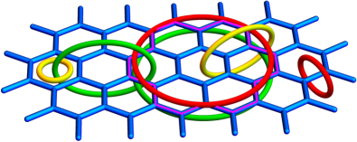
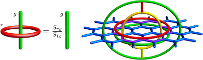
where is the quantum dimension of the string and is the total quantum dimension of the theory considered. The operator injects a closed string around the plaquette and hence “measures” the fluxon state in this plaquette, whereas injects a closed string around the link and “measures” the string state in this link (see Fig. 2 for illustration). In this context, measurement refers to the fundamental relation depicted in Fig. 3 (left), which is reminiscent of the Aharonov-Bohm effect Aharonov and Bohm (1959); Pre . All operators and mutually commute, except when the link belongs to the plaquette .
The Hamiltonian (1) has been first introduced by Gils et al. in the ladder geometry Gils et al. (2009); Gils (see also Refs. Ardonne et al. (2011); Schulz et al. (2015, 2016) for related studies). In the honeycomb lattice considered here, the phase diagram has been the subject of several studies for some specific theories Burnell et al. (2011); Schulz et al. (2013, 2014); Dusuel and Vidal (2015); Schotte et al. (2019).
For , the system is in a topological (string-net condensed Levin and Wen (2005)) phase with a ground-state degeneracy that depends on the surface topology and excitations that are fluxons. By contrast, for , the system is in a trivial (non topological) phase with a unique ground state (all links in the trivial state ) and excitations that are link configurations with nontrivial strings satisfying the branching rules. These two phases are separated by a transition point that depends on the theory considered. In two dimensions, for Abelian theories ( fusion rules), this model has been shown to be equivalent to the quantum Potts model in a transverse field defined on the dual (triangular) lattice Burnell et al. (2011), so that the transition is second-order for and first-order for . For non-Abelian theories, the situation is less clear. First studies based on series expansions and exact diagonalizations indicate a scenario compatible with second-order transitions (at least for Fibonacci Schulz et al. (2013) and Ising theories Schulz et al. (2014)), but the latest mean-field Dusuel and Vidal (2015) and tensor-network approaches Schotte et al. (2019) rather plead in favor of first-order transitions for all cases.
Wegner-Wilson loops.— The Hamiltonian (1) may be seen as a generalization of lattice gauge theories. Indeed, when the input theory is associated to a group, describes a pure gauge theory (no matter) and the transition between the topological and the trivial phase driven by the fluxon dynamics is a deconfinement/confinement transition of the charge excitations. As early proposed Wegner (1971); Wilson (1974), this transition is associated with a change of behavior of the Wegner-Wilson loops that exhibit a perimeter law in the deconfined (topological) phase and an area law in the confined (trivial) phase (see discussion below). The tension of these closed loops informs one about the interaction energy between the excitations existing at the extremities of the corresponding open strings. For instance, in the case, the closed string obtained by creating and annihilating a pair of electric charges and that measures the magnetic flux inside the resulting region, indicates that is responsible for the charge confinement while fluxons condense (see, e.g., Ref. Sachdev (2019) for more discussions).
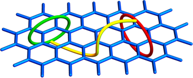
Hence, it is of crucial importance to determine the behavior of the loops. In their original paper, Levin and Wen give the procedure to compute the matrix elements of the Wegner-Wilson loops in the link basis Levin and Wen (2005). As explained in Ref. Burnell and Simon (2010), these expressions are given in terms of symbols and symbols of the input theory. In the fluxon basis, the Wegner-Wilson loop obtained by creating, moving, and annihilating a pair of excitations around a given region of the lattice, is simply represented by two closed strings, and , above and below this region as depicted in Fig. 2. In this representation, these loops can be deformed at will, provided one forbids crossings with nontrivial strings and with links of the honeycomb lattice.
Thus, for , one simply has to evaluate a diagram with loops of type and above and below the lattice in the ground state (no-fluxon state) of the Levin-Wen Hamiltonian. Using graphical rules Kitaev (2003); Bonderson , this directly leads to . As explained above, the ground-state degeneracy in the topological phase depends on the surface topology. The results given here and below are valid for any ground states as long as the region is contractible.
The weak-tension limit: .— To compute in this limit, we use the same method as the one used for the toric code in a magnetic field in Ref. Halász and Hamma (2012). This approach, based on the perturbative continuous unitary transformations (PCUT) Wegner (1994); Głazek and Wilson (1993, 1994); Stein (1997); Knetter and Uhrig (2000); Knetter et al. (2003), provides a clear picture of the various processes contributing to the perturbative corrections. Technically, this perturbative calculation amounts to evaluate diagrams corresponding to virtual excitations [see Fig. 3 (right), for example]. For simplicity, we consider here Wegner-Wilson loops defined on a hexagonal-shape closed region (see Fig. 2). In the perturbative limit where and for sufficiently large , one gets the general structure
| (3) |
where ’s are polynomial of order , and is the number of links defining the contour of (dimensionless perimeter). The first terms of this expansion up to order read
| (4) | |||||
| (5) | |||||
| (6) | |||||
| (7) | |||||
Calculation details will be given elsewhere Vid . These expressions suggest that, in the topological phase, Wegner-Wilson loops obey a perimeter law, i.e., , expected for deconfined phases Kogut (1979) (see Ref. Halász and Hamma (2012) for a similar exponentiation).
The strong-tension limit: .— In this other limiting case, the behavior of the Wegner-Wilson loops is completely different and it is more appropriate to work in the original link basis. For , keeping in mind that the ground state is the product state , where denotes the state in the link , one straightforwardly gets . However, contrary to the topological phase, the first nontrivial contribution occurs at order , where is the number of plaquettes inside the region (dimensionless area). More precisely, one has:
| (8) | |||||
where is a purely combinatorial factor that depends on the region but not on the theory . For instance, if consists in two adjacent plaquettes, one has . This behavior can be interpreted as an area law for the quantity .
Mean-field approach.— It is interesting to compare the results obtained perturbatively with the ones computed from the mean-field ansatz introduced in Ref. Dusuel and Vidal (2015)
| (9) |
where is the normalization constant, is a variational parameter, and . This variational state, which interpolates between one exact ground state for , and the exact ground state for , leads to
| (10) |
where . This mean-field approach relies on a description in terms of decoupled plaquettes which is encoded in the following factorization property Dusuel and Vidal (2015)
| (11) |
In the topological phase, one has and Dusuel and Vidal (2015). Thus, this ansatz yields a trivial perimeter law which corresponds to the leading-order contribution in given in Eq. (3), i.e., . By contrast, in the strong-tension limit (trivial phase), one finds:
| (12) | |||||
| (13) | |||||
| (14) | |||||
Hence, it is remarkable to observe that the mean-field result (14) reproduces the perturbative result (8) with a factor that only depends on the area (but not on the shape) of within this approximation.
Discussion.— Let us now discuss the results that can be inferred from the perturbative calculations. Three cases must be distinguished according to the nature of the strings defining the Wegner-Wilson loops :
-
1.
If and , one can use the following identity (valid for any Abelian strings and ):
(15) to show that . Here, denotes the dual (or conjugate) string of , i.e., Levin and Wen (2005). This is in agreement with the perturbative results given in Eqs. (4)-(8) as well as the mean-field approach [see Eq. (10)]. We conclude that Abelian fluxons are always completely deconfined. In other words, , for all .
- 2.
-
3.
If , depends only on and (at least at the order considered here) and obeys a perimeter law in the topological phase and an area law in the trivial phase.
Perspectives.—
To go beyond the present work, several extensions should be considered. Concerning input theories, one may study the case of UMTCs with nontrivial Frobenius-Schur indicators such as semion or theories Rowell et al. (2009), and/or with nontrivial multiplicities. Input theories that are not UMTCs are also of interest. In that respect, the simplest example is the gauge theory for which there are four Wegner-Wilson loops labeled in Ref. Levin and Wen (2005). It turns out that, in the charge-free sector, , and the expression of can be obtained from Eqs. (4)-(8) by setting , , and . More generally, discrete gauge theories associated to non-Abelian gauge groups (see Ref. Levin and Wen (2005) for a concrete example based on the group) definitely deserve special attention.
Acknowledgements.
We thank S. Dusuel and M. Tissier for fruitful discussions. We are also grateful to M. Mühlhauser and K. P. Schmidt for providing the PCUT coefficients.References
- Wegner (1971) F. Wegner, “Duality in Generalized Ising Models and Phase Transitions without Local Order Parameters,” J. Math. Phys. 12, 2259 (1971).
- Wilson (1974) K. G. Wilson, “Confinement of quarks,” Phys. Rev. D 10, 2445 (1974).
- Kogut and Susskind (1975) J. Kogut and L. Susskind, “Hamiltonian formulation of Wilson’s lattice gauge theories,” Phys. Rev. D 11, 395 (1975).
- Kogut (1979) J. Kogut, “An introduction to lattice gauge theory and spin systems,” Rev. Mod. Phys. 51, 659 (1979).
- Gregor et al. (2011) K. Gregor, D. A. Huse, R. Moessner, and S. L. Sondhi, “Diagnosing deconfinement and topological order,” New J. Phys. 13, 025009 (2011).
- Leinaas and Myrheim (1977) J. M. Leinaas and J. Myrheim, “On the theory of identical particles,” Il Nuovo Cimento B 37, 1 (1977).
- Wilczek (1982) F. Wilczek, “Quantum mechanics of fractional-spin particles,” Phys. Rev. Lett. 49, 957 (1982).
- Kitaev (2003) A. Kitaev, “Fault-tolerant quantum computation by anyons,” Ann. Phys. (NY) 303, 2 (2003).
- Ogburn and Preskill (1999) W. R. Ogburn and J. Preskill, “Topological Quantum Computation,” Lect. Notes Comput. Sci. 1509, 341 (1999).
- Freedman et al. (2003) M. H. Freedman, A. Kitaev, M.J. Larsen, and Wang, “Topological quantum computation,” Bull. Amer. Math. Soc. 40, 31 (2003).
- (11) See http://www.theory.caltech.edu/preskill/ph219/ for a pedagogical introduction.
- Nayak et al. (2008) C. Nayak, S. H. Simon, A. Stern, M. Freedman, and S. Das Sarma, “Non-Abelian Anyons and Topological Quantum Computation,” Rev. Mod. Phys. 80, 1083 (2008).
- (13) Z. Wang, Topological Quantum Computation, CBMS Regional Conference Series in Mathematics, No. 112 (American Mathematical Society, Providence, RI, 2010).
- Wen (2017) X.-G. Wen, “Zoo of quantum-topological phases of matter,” Rev. Mod. Phys. 89, 041004 (2017).
- Levin and Wen (2005) M. A. Levin and X.-G. Wen, “String-net condensation: A physical mechanism for topological phases,” Phys. Rev. B 71, 045110 (2005).
- Turaev and Viro (1992) V. G. Turaev and O. Y. Viro, “State sum invariants of 3-manifolds and quantum -symbols,” Topology 31, 865 (1992).
- Kádár et al. (2010) Z. Kádár, A. Marzuoli, and M.Rasetti, “Microscopic Description of 2D Topological Phases, Duality, and 3D State Sums,” Adv. Math. Phys. 2010, 671039 (2010).
- (18) A. Kirillov, “String-net model of Turaev-Viro invariants,” arXiv:1106.6033.
- Koenig et al. (2010) R. Koenig, G. Kuperberg, and B. W. Reichardt, “Quantum computation with Turaev-Viro codes,” Ann. Phys. (NY) 325, 2707 (2010).
- Witten (1989) E. Witten, “Quantum field theory and the Jones polynomial,” Commun. Math. Phys. 121, 351 (1989).
- Moore and Seiberg (1989) G. Moore and N. Seiberg, “Classical and quantum conformal field theory,” Commun. Math. Phys. 123, 177 (1989).
- Rowell et al. (2009) E. Rowell, R. Stong, and Z. Wang, “On Classification of Modular Tensor Categories,” Commun. Math. Phys. 292, 343 (2009).
- (23) P. H. Bonderson, Ph. D. thesis, California Institute of Technology, (2007).
- (24) Here, we consider only multiplicity-free UMTCs whose labels have trivial Frobenius-Schur indicators.
- Simon and Fendley (2013) S. H. Simon and P. Fendley, “Exactly solvable lattice models with crossing symmetry,” J. Phys. A 46, 105002 (2013).
- Schulz et al. (2013) M. D. Schulz, S. Dusuel, K. P. Schmidt, and J. Vidal, “Topological Phase Transitions in the Golden String-Net Model,” Phys. Rev. Lett. 110, 147203 (2013).
- Schulz et al. (2014) M. D. Schulz, S. Dusuel, G. Misguich, K. P. Schmidt, and J. Vidal, “Ising anyons with a string tension,” Phys. Rev. B 89, 201103 (2014).
- Hu et al. (2018) Y. Hu, N. Geer, and Y.-S. Wu, “Full dyon excitation spectrum in extended Levin-Wen models,” Phys. Rev. B 97, 195154 (2018).
- Aharonov and Bohm (1959) Y. Aharonov and D. Bohm, “Significance of Electromagnetic Potentials in the Quantum Theory,” Phys. Rev. 115, 485 (1959).
- Gils et al. (2009) C. Gils, S. Trebst, A. Kitaev, A. W. W. Ludwig, M. Troyer, and Z. Wang, “Topology-driven quantum phase transitions in time-reversal-invariant anyonic quantum liquids,” Nat. Phys. 5, 834 (2009).
- (31) C. Gils, “Ashkin-Teller universality in a quantum double model of Ising anyons,” J. Stat. Mech., P07019 (2009).
- Ardonne et al. (2011) E. Ardonne, J. Gukelberger, A. W. W. Ludwig, S. Trebst, and M. Troyer, “Microscopic models of interacting Yang-Lee anyons,” New J. Phys. 13, 045006 (2011).
- Schulz et al. (2015) M. D. Schulz, S. Dusuel, and J. Vidal, “Russian doll spectrum in a non-Abelian string-net ladder,” Phys. Rev. B 91, 155110 (2015).
- Schulz et al. (2016) M. D. Schulz, S. Dusuel, and J. Vidal, “Bound states in string nets ,” Phys. Rev. B 94, 205102 (2016).
- Burnell et al. (2011) F. J. Burnell, S. H. Simon, and J. K. Slingerland, “Condensation of achiral simple currents in topological lattice models: Hamiltonian study of topological symmetry breaking,” Phys. Rev. B 84, 125434 (2011).
- Dusuel and Vidal (2015) S. Dusuel and J. Vidal, “Mean-field ansatz for topological phases with string tension,” Phys. Rev. B 92, 125150 (2015).
- Schotte et al. (2019) A. Schotte, J. Carrasco, B. Vanhecke, L. Vanderstraeten, J. Haegeman, F. Verstraete, and J. Vidal, “Tensor-network approach to phase transitions in string-net models,” Phys. Rev. B 100, 245125 (2019).
- Sachdev (2019) S. Sachdev, “Topological order, emergent gauge fields, and Fermi surface reconstruction,” Rep. Prog. Phys. 82, 014001 (2019).
- Burnell and Simon (2010) F. J. Burnell and S. H. Simon, “Space-time geometry of topological phases,” Ann. Phys. (NY) 325, 2550 (2010).
- Halász and Hamma (2012) G. B. Halász and A. Hamma, “Probing topological order with Rényi entropy,” Phys. Rev. A 86, 062330 (2012).
- Wegner (1994) F. Wegner, “Flow equations for Hamiltonians,” Ann. Phys. (Leipzig) 3, 77 (1994).
- Głazek and Wilson (1993) S. D. Głazek and K. G. Wilson, “Renormalization of Hamiltonians,” Phys. Rev. D 48, 5863 (1993).
- Głazek and Wilson (1994) S. D. Głazek and K. G. Wilson, “Perturbative renormalization group for Hamiltonians,” Phys. Rev. D 49, 4214 (1994).
- Stein (1997) J. Stein, “Flow equations and the strong-coupling expansion for the Hubbard model,” J. Stat. Phys. 88, 487 (1997).
- Knetter and Uhrig (2000) C. Knetter and G. S. Uhrig, “Perturbation theory by flow equations: dimerized and frustrated S= 1/2 chain,” Eur. Phys. J. B 13, 209 (2000).
- Knetter et al. (2003) C. Knetter, K. P. Schmidt, and G. S. Uhrig, “The structure of operators in effective particle-conserving models,” J. Phys. A 36, 7889 (2003).
- (47) J. Vidal et al. (unpublished).