Delving Deep into Label Smoothing

Abstract

Label smoothing is an effective regularization tool for deep neural networks (DNNs), which generates soft labels by applying a weighted average between the uniform distribution and the hard label. It is often used to reduce the overfitting problem of training DNNs and further improve classification performance. In this paper, we aim to investigate how to generate more reliable soft labels. We present an Online Label Smoothing (OLS) strategy, which generates soft labels based on the statistics of the model prediction for the target category. The proposed OLS constructs a more reasonable probability distribution between the target categories and non-target categories to supervise DNNs. Experiments demonstrate that based on the same classification models, the proposed approach can effectively improve the classification performance on CIFAR-100, ImageNet, and fine-grained datasets. Additionally, the proposed method can significantly improve the robustness of DNN models to noisy labels compared to current label smoothing approaches. The source code is available at our project page: https://mmcheng.net/ols/ and https://github.com/zhangchbin/OnlineLabelSmoothing

I Introduction

Deep Neural Networks (DNNs) [1, 2, 3, 4, 5, 6, 7] have achieved remarkable performance in image recognition  [8, 9]. However, most DNNs tend to fall into over-confidence for training samples, greatly influencing their generalization ability to test samples. Recently, researchers have proposed many regularization approaches, including Label Smoothing [10], Bootstrap [11], CutOut [12], MixUp [13], DropBlock [14] and ShakeDrop [15], to conquer the overfitting problem to the distribution of the training set. These methods attempt to tackle this problem from the views of data augmentation [12, 13], model design [14, 15], or label transformation [10, 11, 16]. Among them, label smoothing is a simple yet effective regularization tool operating on the labels.

Label smoothing (LS), aiming at providing regularization for a learnable classification model, is first proposed in [10]. Instead of merely leveraging the hard labels for training (Fig. 1(a)), Christian et al.[10] utilizes soft labels by taking an average between the hard labels and the uniform distribution over labels (Fig. 1(b)). Although such kind of soft labels can provide strong regularization and prevent the learned models from being over-confident, it treats the non-target categories equally by assigning them with fixed identical probability. For example, a ‘cat’ should be more like a ‘dog’ rather than an ‘automobile.’ Therefore, we argue that the assigned probabilities of non-target categories should highly consider their similarities to the category of the given image. Equally treating each non-target category could weaken the capability of label smoothing and limit the model performance.

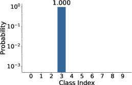
(a) Hard Label

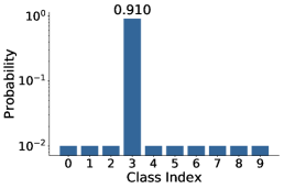
(b) LS

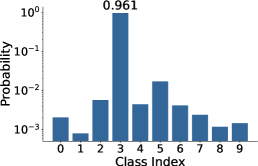
(c) Ours

Figure 1: Different kinds of label distributions on the CIFAR-10 dataset. The target category is ‘cat.’ We scale the $y$-axis using the $log$ function for visualization. (a) Original hard label. (b) Soft label generated by LS [10]. This soft label is a mixture of the hard label and uniform distribution. (c) Soft label generated by our OLS method during the training process of ResNet-29.

0 – airplane       1 – automobile       2 – bird       3 – cat       4 – deer       5 – dog       6 – frog       7 – horse       8 – ship       9 – truck

It has been demonstrated in [17] that model predictive distributions provide a promising way to reveal the implicit relationships among different categories. Motivated by this knowledge, we propose a simple yet effective method to generate more reliable soft labels that consider the relationships among different categories to take the place of label smoothing. Specifically, we maintain a moving label distribution for each category, which can be updated during the training process. The maintained label distributions keep changing at each training epoch and are utilized to supervise DNNs until the model reaches convergence. Our method takes advantage of the statistics of the intermediate model predictions, which can better build the relationships between the target categories and the non-target ones. It can be observed from Fig. 1(c) that our method gives more confidence to the animal categories instead of those non-animal ones when the label is ‘cat.’

We conduct extensive experiments on CIFAR-100, ImageNet [9] and four fine-grained datasets [18, 19, 20, 21]. Our OLS can make consistent improvements over baselines. To be specific, directly applying OLS to ResNet-56 and ResNeXt29-2x64d yields 1.57% and 2.11% top-1 performance gains on CIFAR-100, respectively. For ImageNet, our OLS can bring 1.4% and 1.02% performance improvements to ResNet-50 and ResNet-101 [2], respectively. On four fine-grained datasets, OLS achieves an average 1.0% performance improvement over LS [10] on four different backbones, i.e., ResNet-50 [2], MobileNetv2 [6], EfficientNet-b7 [22] and SAN-15 [23]. The proposed OLS can be naturally employed to tackle noisy labels by reducing the overfitting to training sets. Additionally, OLS can be conveniently used in the training process of many models. We hope it can serve as an effective regularization tool to augment the training of classification models.

II Related Work

TABLE I: Comparison between our method and knowledge distillation. Self-KD denotes self-Knowledge Distillation.

	Vanilla KD [17]	Arch.-based self-KD [24]	Data-based self-KD [25]	OLS (Ours)
Label	sample-level	sample-level	sample-level	class-level
Trained teacher model	✓	✗	✗	✗
Special network architecture	✗	✓	✗	✗
Forward times in one training iteration	2	1	2	1

Regularization tools on labels. Training DNNs with hard labels (assigning 1 to the target category and 0 to the non-target ones) often results in over-confident models. Boosting labels is a straightforward yet effective way to alleviate the overfitting problem and improve the accuracy and robustness of DNNs. Bootstrapping [11] provided two options, Bootsoft and Boothard, which smoothed the hard labels using the predicted distribution and the predicted class, respectively. Xie et al. [26] randomly perturbed labels of some samples in a mini-batch to regularize the networks. To further prevent the training models from overfitting to some specific samples, Dubey et al. [27] added pairwise confusion to the output logits of samples belonging to different categories in training so that the models can learn slightly less discriminative features for specific samples. Li et al. [28] used two networks to embed the images and the labels in a latent space and regularize the network via the distance between these embeddings. Christian et al. [10] leveraged soft labels for training, where the soft labels are generated by taking an average between the hard labels and the uniform distribution over labels. Our OLS also focuses on generating soft labels that can provide stable regularization for models. Following AET [29, 30] and AVT [31], Wang et al. [32] proposed an innovative framework, EnAET [32], that combined semi-supervised and self-supervised training. It learned feature representation by predicting non-spatial and spatial transformation parameters. Both our method and EnAET [32] obtained soft labels by accumulating predictions of multiple samples. However, our method is very different from EnAET [32]. It obtained soft labels by accumulating the augmented views of the same sample by different transformation functions. This consistency constraint is also often used in self-Knowledge Distillation. In contrast, our method is to encourage the predictions of all samples in the same class to become consistent by the accumulated class-level soft labels. Unlike the mentioned approaches above, the soft labels generated by OLS take advantage of the statistical characteristics of model predictions of intermediate states.

Knowledge distillation. Knowledge distillation [17, 33, 34], is a popular way to compress models, which can significantly improve the performance of light-weight networks. Knowledge distillation has been widely used in many tasks [35, 36, 37, 38]. Hinton et al. [17] show that the success of knowledge distillation is due to the model’s response to the non-target classes. It shows that DNNs can discover the similarities among different categories [17, 34] hidden in the predictions. Inspired by knowledge distillation, some works [24, 25, 34] utilized a self-distillation strategy to improve classification accuracy. BYOT [24] designed a network architecture-based self-Knowledge Distillation, which distilled the knowledge from the deep layers to the shallow layer. Xu et al. [25] applied a data-based self-Knowledge Distillation and encouraged the output of the augmented samples (using data augmentation methods) to be consistent with the original samples. Furlanello et al. [34] proposed to distill the knowledge of the teacher model to the student model with the same architecture. The student model obtained a higher accuracy than the teacher model. At the same time, Tommaso et al. [34] also verified the importance of the similarity between categories in the soft labels. Our work is inspired by knowledge distillation, aiming to find a reasonable similarity among categories. Both knowledge distillation and our method use the output logits of the network as soft labels and benefit from the similarities hidden in the logits [17, 34]. But there are many differences between our method and the knowledge distillation. We summarize the main differences in Tab. I. Without any teacher models, compared with knowledge distillation, our method could save the training cost, i.e., our method does not bring extra forward propagations. Besides, our method is applicable to any network architecture without special modification.

Classification against noisy labels. Noisy labels in current datasets are inevitable due to the incorrect annotations by humans. To deal with this problem, many researchers explored solutions to this problem from both models [39, 40], data [41, 42] and training strategies [43, 44, 45]. A typical idea [46, 47, 48] is to weight different samples to reduce the influence of noisy samples on training. Ren et al. [46] verified each mini-batch on the clean validation set to adjust each sample’s weight in a mini-batch dynamically. MetaWeightNet [47] also exploited the clean validation set to learn the weights for samples by a multilayer perceptron (MLP). Moreover, some researchers solve this problem from the optimization perspective [49, 50]. Wang et al. [49] improved the robustness against noisy labels by replacing the normal cross-entropy function with the symmetric cross-entropy function. Arazo et al. [51] observed that noisy samples often have higher losses than the clean ones during the early epochs of training. Based on this observation, they proposed to use the beta mixture model to represent clean samples and noisy samples and adopt this model to provide estimates of the actual class for noisy samples. Another kind of idea [52, 53] is to train the network with only the right labels. PENCIL [54] proposed a novel framework to learn the correct label and model’s weights at the same time. This method maintained a learnable label for each sample. Han et al. [45] designed the label correction phase and performed the training phase and label correction phase iteratively. They got multiple prototypes for each class and redefined the labels for all samples. Different from these two methods, our method does not specifically design the process of label correction. Therefore, our method does not bring extra learnable parameters and does not conflict with the label correction strategy designed in Han et al. [45]. On the other hand, we accumulate the output of correctly predicted samples during training to get the soft labels for each class. These soft labels bring intra-class constraints to reduce the over-fitting to the wrong labels, which improves the robustness to noisy labels. Although the proposed OLS is not specifically designed for noisy labels, the classification accuracy on noisy datasets is largely improved when training models with OLS. The performance gain owes to the ability of OLS to reduce the overfitting to noisy samples.

\begin{overpic}[width=433.62pt,tics=2]{pipeline/pipeline_v7_crop.pdf} \put(22.5,18.7){{Supervise}} \put(23.3,6.7){{Update}} \par{\color[rgb]{0.45,0.45,0.45}\put(32.4,6.5){$S^{1}$}} \put(35.4,6.5){$S^{2}$} {\color[rgb]{0.45,0.45,0.45} \put(38.4,6.5){$S^{3}$} \put(41.4,6.5){$\cdot$} \put(41.8,6.5){$\cdot$} \put(42.2,6.5){$\cdot$} \put(43.6,6.5){$S^{t}$} \put(46.4,6.5){$\cdot$} \put(46.8,6.5){$\cdot$} \put(47.2,6.5){$\cdot$} \put(48.8,6.5){$S^{T}$} } \par{\color[rgb]{0.45,0.45,0.45} \put(32.0,18.5){$S^{0}$} } \put(35.0,18.5){$S^{1}$} {\color[rgb]{0.45,0.45,0.45} \put(38.0,18.5){$S^{2}$} \put(41.0,18.5){$\cdot$} \put(41.4,18.5){$\cdot$} \put(41.8,18.5){$\cdot$} \put(42.5,18.5){$S^{t-1}$} \put(46.2,18.5){$\cdot$} \put(46.6,18.5){$\cdot$} \put(47.0,18.5){$\cdot$} \put(48.0,18.5){$S^{T-1}$} } \par\put(26.0,12.6){{epoch}} {\color[rgb]{0.45,0.45,0.45} \put(32.0,12.6){$\#$1} } \put(35.0,12.6){$\#${2}} {\color[rgb]{0.45,0.45,0.45} \put(38.0,12.6){$\#3$} \put(41.0,12.6){$\cdot$} \put(41.4,12.6){$\cdot$} \put(41.8,12.6){$\cdot$} \put(43.0,12.6){$\#t$} \put(46.2,12.6){$\cdot$} \put(46.6,12.6){$\cdot$} \put(47.0,12.6){$\cdot$} \put(47.6,12.67){$\#T$} } \put(56.4,24.7){{Supervise}} \put(67.0,0.3){{Update}} \par\put(68.7,24.0){$S^{1}$} \put(88.7,24.0){$S^{2}$} \par\put(14.0,2.0){Predicted category: 1} \put(14.0,0.0){Ground-Truth: 1} \par\put(60.8,2.0){0} \put(64.2,2.0){1} \put(67.6,2.0){2} \put(71.0,2.0){$\cdots$} \put(76.0,2.0){$K$} \par\put(81.5,2.0){0} \put(85.0,2.0){1} \put(88.5,2.0){2} \put(91.7,2.0){$\cdots$} \put(96.7,2.0){$K$} \par\end{overpic}

Figure 2: The illustration of training DNN with our online label smoothing method. The left part of the figure shows the whole training process. We simply divided the training process into T phases according to the training epochs. $K$ denotes the number of categories in datasets. We define each column of $S^{t}$ to represent the soft label for a target category. At each epoch, we use the soft labels generated in the previous epoch to supervise the model, and meanwhile, we generate the soft labels for the next epoch. In the right, we show a detailed example of the training process in epoch$\#2$. The generation of $S^{t}$ is depicted in Sec. III.

III Method

III-A Preliminaries

Given a dataset $\mathcal{D}_{\tt train}=\{(\bm{x_{i}},y_{i})\}$ with $K$ classes, where $\bm{x_{i}}$ denotes the input image and $y_{i}$ denotes the corresponding ground-truth label. For each sample $(\bm{x_{i}},y_{i})$, the DNN model predicts a probability $p(k|\bm{x_{i}})$ for the class $k$ using the softmax function. The distribution $q$ of the hard label $y_{i}$ can be denoted as $q(k=y_{i}|\bm{x_{i}})=1$ and $q(k\neq y_{i}|\bm{x_{i}})=0$. Then, the standard cross-entropy loss used in image classification for $(\bm{x_{i}},y_{i})$ can be written as

$$L_{hard}=-\sum_{k=1}^{K}q(k|\bm{x_{i}})\log{p(k|\bm{x_{i}})}$$ (1)

$$=-\log{p(k=y_{i}|\bm{x_{i}})}.$$

Instead of using hard labels for model training, LS [10] utilizes soft labels that are generated by exploiting a uniform distribution to smooth the distribution of the hard labels. Specifically, the probability of $\bm{x_{i}}$ being class $k$ in the soft label can be expressed as

$$q^{\prime}(k|\bm{x_{i}})=(1-\varepsilon)q(k|\bm{x_{i}})+\frac{\varepsilon}{K},$$ (2)

where $\varepsilon$ denotes the smoothing parameter that  is usually set to 0.1 in practice. The assumption behind LS is that the confidence for the non-target categories is treated equally as shown in Fig. 1(b). Although combining the uniform distribution with the original hard label is useful for regularization, LS itself does not consider the genuine relationships among different categories [55]. We take this into account and present our online label smoothing method accordingly.

III-B Online Label Smoothing

According to knowledge distillation, the similarity among categories can be effectively discovered from the model predictions [34, 17]. Motivated by this fact, unlike LS utilizing a static soft label, we propose to exploit model predictions to continuously update the soft labels during the training phase. Specifically, in the training process, we maintain a class-level soft label for each category. Given an input image $\bm{x_{i}}$, if the classification is correct, the soft label corresponding to the target class $y_{i}$ will be updated using the predicted probability $p(\bm{x_{i}})$. Then the updated soft labels will be subsequently utilized to supervise the model. The pipeline of our proposed method is shown in Fig. 2.

Formally, let $T$ denote the number of training epochs. We then define $\mathcal{S}=\{S^{0},S^{1},\cdots,S^{t},\cdots,S^{T-1}\}$ as the collection of the class-level soft labels at different training epochs. Here, $S^{t}$ is a matrix with $K$ rows and $K$ columns, and each column in $S^{t}$ corresponds to the soft label for one category. In the $t_{th}$ training epoch, given a sample $(\bm{x_{i}},y_{i})$, we use the soft label $S^{t-1}_{y_{i}}$ to form a temporary label distribution to supervise the model, where $S^{t-1}_{y_{i}}$ denotes the soft label for the target category $y_{i}$. The training loss of the model supervised by $S^{t-1}_{y_{i}}$ for $(\bm{x_{i}},y_{i})$ can be represented by

$$L_{soft}=-\sum_{k=1}^{K}S^{t-1}_{y_{i},k}\cdot\log{p(k|\bm{x_{i}})}.$$ (3)

It is possible that we directly use the above soft label to supervise the training model, but we find that the model is hard to converge due to the random parameter initialization at the beginning and the lack of the hard label. Thus, we utilize both the hard label and soft label as supervision to train the model. Now, the total training loss can be represented by

$$L=\alpha L_{hard}+(1-\alpha)L_{soft},$$ (4)

where $\alpha$ is used to balancing $L_{hard}$ and $L_{soft}$.

Algorithm 1 The pipeline of the proposed OLS

  Input: Dataset $\mathcal{D}_{\tt train}=\{(\bm{x_{i}},y_{i})\}$, model $f_{\theta}$, training epochs $T$

  Initialize: Soft label matrix $\bm{S^{0}}=\frac{1}{K}\bm{I}$, $\bm{I}$ denotes unit matrix, $K$ denotes the number of classes

  for current epoch $t=1$ to $T$ do

     Initialize: $\bm{S^{t}}=\bm{0}$

     for $iter=1$ to $iterations$ do

        Sample a batch $\mathcal{B}\subset\mathcal{D}_{\tt train}$, input to $f_{\theta}$

        Obtain predicted probabilities $\{f(\theta,\bm{x_{i}}),\bm{x_{i}}\in\mathcal{B}\}$

        Compute loss by Eqn. (4), backward to update the parameter $\theta$

        for $i=1$ to $|\mathcal{B}|$ do

           Update $\bm{S_{y_{i}}^{t}}\leftarrow\bm{S_{y_{i}}^{t}}+f(\theta,\bm{x_{i}})$

        end for

     end for

     Normalize $\bm{S^{t}}$ at each column

  end for

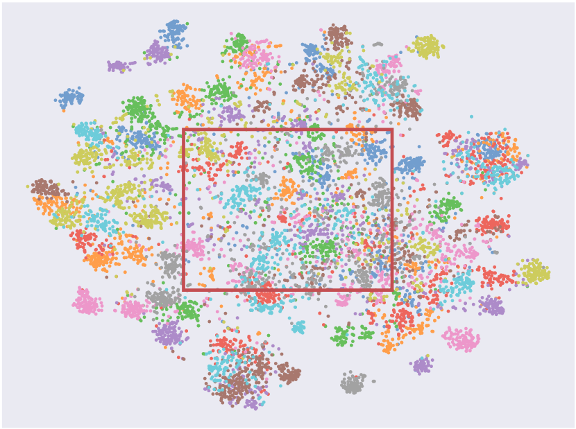
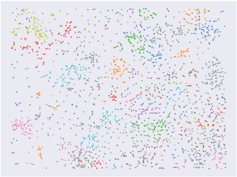
(a) Hard Label

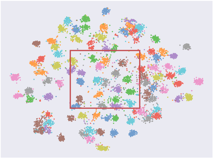
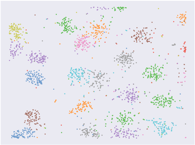
(b) Label Smoothing (LS)

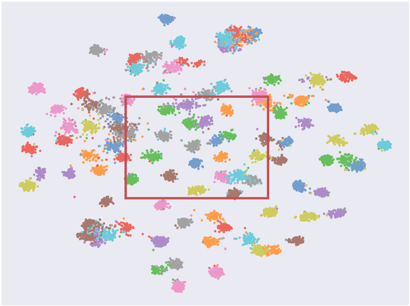
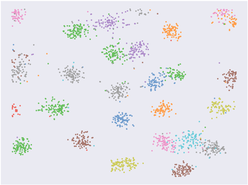
(c) OLS (Ours)

Figure 3: Visualization of the penultimate layer representations of ResNet-56 on CIFAR-100 training set using t-SNE [56]. Note that we use the same color for every 10 classes. We visualize the representations of all 100 classes (top). We zoom the patch in red boxes for better visualization. (bottom).

In the $t_{th}$ training epoch, we also use the predicted probabilities of the input samples to update $S^{t}_{y_{i}}$, which will be utilized to supervise the model training in the $t+1$ epoch. At the beginning of the $t_{th}$ training epoch, we initialize the soft label $S^{t}$ as a zero matrix. When an input sample $(\bm{x_{i}},y_{i})$ is correctly classified by the model, we utilize its predicted score $p(\bm{x_{i}})$ to update the $y_{i}$ column in $S_{t}$, which can be formulated as

$$S_{y_{i},k}^{t}=S_{y_{i},k}^{t}+p(k|\bm{x_{i}}),$$ (5)

where $k\in\{1,\cdots,K\}$, indexing the soft label $S_{y_{i}}^{t}$. At the end of the $t_{th}$ training epoch, we normalize the cumulative $S^{t}$ column by column as represented by

$$S_{y_{i},k}^{t}\leftarrow\frac{S_{y_{i},k}^{t}}{\sum_{l=1}^{K}S_{y_{i},l}^{t}}.$$ (6)

We can now obtain the normalized soft label $S^{t}$ for all $K$ categories, which will be used to supervise the model at the next training epoch. Notice that we cannot obtain the soft label at the first epoch. Thus, we use the uniform distribution to initialize each column in $S^{0}$. More details for the proposed approach are described in Algorithm 1.

Discussion

The soft label $S^{t-1}_{y_{i},k}$ generated from the $t-1$ epoch can be denoted as

$$S^{t-1}_{y_{i},k}=\frac{1}{N}\sum_{j=1}^{N}p^{t-1}(k|\bm{x_{j}}),$$ (7)

where $N$ denotes the number of correctly predicted samples with label $y_{i}$. $p^{t-1}(k|\bm{x_{j}})$ is the output probability of category $k$ when input $x_{j}$ to the network at the $t-1$ epoch. Then Eqn. (3) can be rewritten as

$$L_{soft}=-\sum_{k=1}^{K}\frac{1}{N}\sum_{j=1}^{N}p^{t-1}(k|\bm{x_{j}})\cdot\log{p(k|\bm{x_{i}})}$$ (8)

$$=-\frac{1}{N}\sum_{j=1}^{N}\sum_{k=1}^{K}p^{t-1}(k|\bm{x_{j}})\cdot\log p(k|\bm{x_{i}}).$$

This equation indicates that all correctly classified samples $\bm{x_{j}}$ will impose a constraint to the current sample $\bm{x_{i}}$. The constrain encourages the samples belonging to the same category to be much closer. To give a more intuitive explanation, we utilize t-SNE [56] to visualize the penultimate layer representations of ResNet-56 on CIFAR-100 trained with the hard label, LS, and OLS, respectively. Fig. 3 shows that our proposed method provides a more recognizable difference between representations of different classes and tighter intra-class representations.

Besides, our method does not have the problem of training divergence in the early stages of training. This is because we use a uniform distribution as the soft label in the first epoch of training, which is equivalent to the vanilla label smoothing. In the entire training process afterwards, we only accumulate correct predictions, which guarantees the correctness of the generated soft labels.

TABLE II: Comparison between our method and the state-of-the-art approaches. We run each method three times on CIFAR-100 and compute the mean and standard deviation of the Top-1 Error (%). Best results are highlighted in bold.

Method	ResNet-34	ResNet-50	ResNet-101	ResNeXt29-2x64d	ResNeXt29-32x4d
Hard Label	20.62 $\pm$ 0.21	21.21 $\pm$ 0.25	20.34 $\pm$ 0.40	20.92 $\pm$ 0.52	20.85 $\pm$ 0.17
Bootsoft [11]	21.65 $\pm$ 0.13	21.25 $\pm$ 0.67	20.37 $\pm$ 0.07	21.20 $\pm$ 0.13	20.86 $\pm$ 0.24
Boothard [11]	22.58 $\pm$ 0.02	20.81 $\pm$ 0.13	21.46 $\pm$ 0.22	21.00 $\pm$ 0.10	21.47 $\pm$ 0.59
Disturb Label [26]	20.91 $\pm$ 0.30	22.12 $\pm$ 0.51	20.99 $\pm$ 0.12	21.64 $\pm$ 0.24	21.69 $\pm$ 0.06
SCE [49]	22.86 $\pm$ 0.08	22.12 $\pm$ 0.11	22.60 $\pm$ 0.64	23.07 $\pm$ 0.28	22.96 $\pm$ 0.09
LS [10]	20.94 $\pm$ 0.08	21.20 $\pm$ 0.25	20.12 $\pm$ 0.02	20.34 $\pm$ 0.24	19.56 $\pm$ 0.18
Pairwise Confusion [27]	22.91 $\pm$ 0.04	23.09 $\pm$ 0.53	22.73 $\pm$ 0.39	21.55 $\pm$ 0.11	21.74 $\pm$ 0.04
Xu et al. [25]	22.65 $\pm$ 0.09	22.05 $\pm$ 0.43	21.70 $\pm$ 0.77	22.81 $\pm$ 0.08	23.14 $\pm$ 0.04
OLS	20.04 $\pm$ 0.11	20.65 $\pm$ 0.14	19.66 $\pm$ 0.15	18.81 $\pm$ 0.45	18.79 $\pm$ 0.20
BYOT [24]	20.41 $\pm$ 0.10	19.20 $\pm$ 0.30	18.51 $\pm$ 0.49	19.69 $\pm$ 0.12	20.33 $\pm$ 0.19
BYOT [24] + OLS	19.44 $\pm$ 0.09	18.15 $\pm$ 0.21	18.14 $\pm$ 0.08	18.29 $\pm$ 0.20	19.25 $\pm$ 0.29

IV Discussion

Comparison with Tf-KD [57]. The output of the teacher model in Label Smoothing [10] is a uniform distribution. Yuan et al. [57] argue that this uniform distribution could not reflect the correct class information, so they propose a teacher-free knowledge distillation method, called Tf-KD_reg. They design a teacher with correct class information. The output of the teacher model can be denoted as:

$$u(k)=\begin{cases}a&\text{ if }k=c\\ \frac{1-a}{K-1}&\text{ if }k\neq c\end{cases}$$ (9)

where $u(k)$ is the hand-designed distribution, $c$ is the correct class and $K$ is the number of classes. They set the hyper-parameter $a>0.9$. Although both this distribution and our method could contain the correct class information, the hand-designed distribution of Tf-KD_reg is still uniform distribution among non-target classes. The distribution of Tf-KD [57] still does not imply similarities between classes. On the contrary, our motivation is to find a non-uniform distribution that can reflect the relationship between classes. Hinton et al. [17], Borns Again Network [34] and Tf-KD [57] have emphasized this view that knowledge distillation benefits from the similarities among classes implied in the output of the teacher model. We conduct experiments on four fine-grained datasets as shown in Tab. VI. Our method benefits from the similarities between classes, so it can perform better than Tf-KD [57].

TABLE III: The Top-1 Error of model ensemble. We integrate 6, 10, 15, and 20 models trained at different epochs, respectively. The models are selected uniformly from all training epochs (300 epochs).

Method	1 Model	6 Models	10 Models	15 Models	20 Models
HardLabel	26.41	26.07	25.93	25.87	25.88
LS [10]	26.37	25.30	25.11	24.97	24.96
OLS (ours)	25.27	24.52	24.22	24.10	23.91

Connection with the model ensemble. Integrating models trained at different epochs is an effective and cost-saving ensemble method. The way to integrate the outputs of models trained at different epochs is described as follows:

$$z_{i}=\frac{1}{||T||}\sum_{t\in T}softmax(W(x_{i}|\theta_{t})),$$ (10)

where $z_{i}$ denotes the ensemble predictions, $T$ denotes the set of selected models in different epochs, $W$ denotes the network, $\theta_{t}$ denotes the network parameters in t-th epoch and $x_{i}$ denotes the input sample. Both our method and the model ensemble utilize the knowledge from different training epochs. The model ensemble averages the outputs of models at different epochs to make predictions. However, different from the ensemble method, our method utilize the knowledge from the previous epoch to help the learning in the current epoch. Specifically, our method generates the soft labels in one training epoch, and the soft labels are used to supervise the network training. It is worth noting that our method does not conflict with this ensemble strategy. To verify this point, we conduct experiments on CIFAR-100 using ResNet-56. We apply the same experimental setup described in the Sec. V. Experimental results are shown in Tab. III. For all methods, we apply the same ensemble strategy. We select models uniformly from the whole training schedule (300 epochs). We choose 6, 10, 15 and 20 models for ensemble respectively. In Tab. III, our method achieves 25.27% Top-1 Error. When our method equipping with the ensemble method, the performance is further improved by a large margin (‘20 Models’: 23.91%). The experiments show that there is no conflict between our method and the model ensemble.

V Experiments

In Sec. V-A, we first present and analyze the performance of our approach on CIFAR-100, ImageNet, and some fine-grained datasets. Then, we test the tolerance to symmetric noisy labels in Sec. V-B and robustness to adversarial attacks in Sec. V-C, respectively. In Sec. V-D, we apply our OLS to object detection. Moreover, in Sec. V-E, we conduct extensive ablation experiments to analyze the settings of our method. All the experiments are implemented based on PyTorch [58] and Jittor [59].

V-A General Image Recognition

CIFAR Classification. First, we conduct experiments on CIFAR-100 dataset to compare our OLS with other related methods, including regularization methods on labels (Bootstrap [11], Disturb Label [26], Symmetric Cross Entropy [49], Label Smoothing [10] and Pairwise Confusion [27]) and self-knowledge distillation methods (Xu et al. [25] and BYOT [24]). For a fair comparison with them, we keep the same experimental setup for all methods. Specifically, we train all the models for 300 epochs with a batch size of 128. The learning rate is initially set to 0.1 and decays at the 150$th$ and 225$th$ epoch by a factor of 0.1, respectively. For other hyper-parameters in different methods, we keep their original settings. Additionally, for a fair comparison with BYOT [24] and Xu et al. [25], we remove the feature-level supervision in them and only use the class labels to supervise models.

Tab. II shows the classification results of each method based on different network architectures. It can be seen that our method significantly improves the classification performance on both lightweight and complex models, which indicates its robustness to different networks. Since BYOT [24] is learned with deep supervision, it performs better on deeper models, like ResNet-50 and ResNet-101, than our method. However, our method can be easily plugged into BYOT [24] and achieves better results than BYOT on deeper models. In addition, comparing to LS [10], our method achieves stable improvement on different models. Especially, our method outperforms LS by about 1.5% on ResNeXt29-2x64d. We argue that the performance gain owes to the useful relationships among categories discovered by our soft labels. In Sec. V-E, we will further analyze the importance of building relationships among categories.

ImageNet Classification. We also evaluate our method on a large-scale dataset, ImageNet. It contains 1K categories with a total of 1.2M training images and 50K validation images. Specifically, we use the SGD optimizer to train all the models for 250 epochs with a batch size of 256. The learning rate is initially set to 0.1 and decays at the 75$th$, 150$th$, and 225$th$ epochs, respectively. We report the best performance of each method.

The classification performance on ImageNet dataset is shown in Tab. IV. Applying our OLS to ResNet-50 achieves 22.28% Top-1 Error, which is better than the result with LS [10] by 0.54%. Additionally, ResNet-101 with our OLS can achieve 20.85% top-1 error, which improves ResNet-101 by 1.02% and ResNet-101 with LS by 0.42%, respectively. This demonstrates that our OLS still performs well on the large-scale dataset. Moreover, we explore the combination of our method with other strategies, i.e., data augmentation (CutOut [12]) and self-distillation (BYOT [24]). In Tab. IV, we observe the combination with them brings extra performance gains to ResNet50 and ResNet101. Our OLS can be utilized as a plug-in regularization module, which is easy to be combined with other methods.

TABLE IV: Classification results on ImageNet. $\ddagger$ denotes the results reported in Tf-KD [57].

Model	Top-1 Error(%)	Top-5 Error(%)
ResNet-50	24.23‡	-
ResNet-50 + LS [10]	23.62‡	-
ResNet-50 + Tf-KDself [57]	23.59‡	-
ResNet-50 + Tf-KDreg [57]	23.58‡	-
ResNet-50	23.68	7.05
ResNet-50 + Bootsoft [11]	23.49	6.85
ResNet-50 + Boothard [11]	23.85	7.07
ResNet-50 + LS [10]	22.82	6.66
ResNet-50 + CutOut [12]	22.93	6.66
ResNet-50 + Disturb Label [26]	23.59	6.90
ResNet-50 + BYOT [24]	23.04	6.51
ResNet-50 + OLS	22.28	6.39
ResNet-50 + CutOut [12] + OLS	21.98	6.18
ResNet-50 + BYOT [24] + OLS	21.88	6.27
ResNet-101	21.87	6.29
ResNet-101 + LS [10]	21.27	5.85
ResNet-101 + CutOut [12]	20.72	5.51
ResNet-101 + OLS	20.85	5.50
ResNet-101 + CutOut [9] + LS [10]	20.47	5.51
ResNet-101 + CutOut [9] + OLS	20.25	5.42

TABLE V: Detailed information of the fine-grained datasets.

Dataset	Categories	Training Samples	Test Samples
CUB-200-2011 [19]	200	5994	5794
Flowers-102 [18]	102	2040	6149
Cars [20]	196	8144	8041
Aircrafts [21]	90	6667	3333

TABLE VI: The Top-1 and Top-5 Error(%) of different architectures on fine-grained classification datasets. All results are averaged over three runs. The $\triangle$ denotes the average improvement relative to Hard Label on all datasets and backbones.

Dataset	Backbones	Hard Label		LS [10]		Tf-KD [57]		OLS
		Top-1 Err(%)	Top-5 Err(%)	Top-1 Err(%)	Top-5 Err(%)	Top-1 Err(%)	Top-5 Err(%)	Top-1 Err(%)	Top-5 Err(%)
CUB-200-2011 [19]	ResNet-50 [2]	$19.19\pm 0.22$	$5.00\pm 0.25$	$18.11\pm 0.14$	$4.88\pm 0.08$	$19.04\pm 0.23$	$4.92\pm 0.16$	$17.53\pm 0.09$	$4.01\pm 0.27$
Flowers-102 [18]		$9.31\pm 0.19$	$2.43\pm 0.14$	$7.58\pm 0.07$	$1.93\pm 0.03$	$8.70\pm 0.45$	$2.46\pm 0.09$	$7.14\pm 0.14$	$1.55\pm 0.07$
Cars [20]		$9.58\pm 0.19$	$1.79\pm 0.01$	$8.32\pm 0.09$	$1.57\pm 0.03$	$8.65\pm 0.16$	$1.46\pm 0.10$	$7.46\pm 0.01$	$0.92\pm 0.04$
Aircrafts [21]		$11.88\pm 0.11$	$3.86\pm 0.13$	$9.92\pm 0.07$	$3.73\pm 0.12$	$10.55\pm 0.22$	$3.34\pm 0.21$	$9.19\pm 0.12$	$2.60\pm 0.03$
CUB-200-2011 [19]	MobileNetv2 [6]	$22.24\pm 0.33$	$6.61\pm 0.21$	$21.33\pm 0.29$	$7.05\pm 0.09$	$22.36\pm 0.27$	$6.41\pm 1.47$	$20.05\pm 0.11$	$5.08\pm 0.12$
Flowers-102 [18]		$8.97\pm 0.09$	$2.51\pm 0.19$	$8.06\pm 0.35$	$2.46\pm 0.08$	$8.05\pm 0.14$	$2.23\pm 0.13$	$7.27\pm 0.17$	$1.77\pm 0.10$
Cars [20]		$11.71\pm 0.13$	$2.29\pm 0.12$	$10.17\pm 0.07$	$2.33\pm 0.05$	$10.57\pm 0.09$	$2.14\pm 0.04$	$9.25\pm 0.05$	$1.33\pm 0.02$
Aircrafts [21]		$13.16\pm 0.33$	$4.15\pm 0.19$	$12.05\pm 0.29$	$4.08\pm 0.17$	$11.95\pm 0.27$	$4.04\pm 0.10$	$10.53\pm 0.25$	$2.96\pm 0.15$
CUB-200-2011 [19]	EfficientNet-b7 [22]	$18.44\pm 0.15$	$5.07\pm 0.13$	$17.40\pm 0.14$	$5.02\pm 0.03$	$20.24\pm 0.09$	$6.33\pm 0.21$	$16.21\pm 0.24$	$3.34\pm 0.02$
Flowers-102 [18]		$9.50\pm 0.07$	$2.04\pm 0.07$	$9.42\pm 0.34$	$2.34\pm 0.13$	$8.58\pm 0.37$	$2.07\pm 0.10$	$8.16\pm 0.12$	$1.63\pm 0.15$
Cars [20]		$9.24\pm 0.22$	$1.84\pm 0.13$	$8.42\pm 0.08$	$1.76\pm 0.07$	$9.52\pm 0.01$	$1.64\pm 0.01$	$7.53\pm 0.13$	$0.97\pm 0.02$
Aircrafts [21]		$11.61\pm 0.37$	$3.72\pm 0.20$	$9.60\pm 0.15$	$3.62\pm 0.13$	$9.45\pm 0.49$	$2.01\pm 0.04$	$8.83\pm 0.19$	$2.71\pm 0.12$
CUB-200-2011 [19]	SAN-15 [23]	$19.05\pm 0.39$	$5.37\pm 0.25$	$17.54\pm 0.30$	$5.43\pm 0.19$	$19.88\pm 0.17$	$5.81\pm 0.03$	$17.28\pm 0.14$	$4.08\pm 0.07$
Flowers-102 [18]		$7.85\pm 0.29$	$1.78\pm 0.21$	$8.08\pm 0.34$	$1.95\pm 0.15$	$7.87\pm 0.43$	$1.91\pm 0.28$	$7.09\pm 0.18$	$1.56\pm 0.12$
Cars [20]		$9.23\pm 0.07$	$1.78\pm 0.02$	$8.55\pm 0.15$	$1.87\pm 0.04$	$8.98\pm 0.07$	$1.76\pm 0.14$	$7.55\pm 0.14$	$1.08\pm 0.07$
Aircrafts [21]		$11.31\pm 0.13$	$3.79\pm 0.08$	$9.96\pm 0.09$	$3.45\pm 0.14$	$10.77\pm 0.03$	$4.18\pm 0.08$	$9.43\pm 0.08$	$2.95\pm 0.09$
Average Improvements ($\triangle$)		0.00	0.00	1.11 $\uparrow$	0.02 $\uparrow$	0.44 $\uparrow$	0.19 $\uparrow$	2.00 $\uparrow$	0.96 $\uparrow$

TABLE VII: The classification performance of different methods under different noisy rates. We run each method three times under different noisy rates and compute the mean and standard deviation of the Top-1 Error(%). The best two results are in bold.

Method/Noise Rate	0%	20%	40%	60%	80%
Hard Label	26.81 $\pm$ 0.36	37.75 $\pm$ 0.50	47.07 $\pm$ 1.08	62.06 $\pm$ 0.62	81.56 $\pm$ 0.42
Bootsoft [11]	27.28 $\pm$ 0.35	37.99 $\pm$ 0.43	46.96 $\pm$ 0.33	63.76 $\pm$ 0.85	80.32 $\pm$ 0.33
Boothard [11]	26.02 $\pm$ 0.22	36.21 $\pm$ 0.29	42.73 $\pm$ 0.16	54.95 $\pm$ 2.20	81.20 $\pm$ 1.26
Symmetric Cross Entropy [49]	28.97 $\pm$ 0.31	38.40 $\pm$ 0.12	46.97 $\pm$ 0.65	62.13 $\pm$ 0.55	82.66 $\pm$ 0.10
Ren et al.[46]	38.38 $\pm$ 0.35	43.74 $\pm$ 1.21	49.83 $\pm$ 0.53	57.65 $\pm$ 0.98	73.04 $\pm$ 0.15
MetaWeightNet [47]	29.51 $\pm$ 0.51	35.06 $\pm$ 0.48	43.58 $\pm$ 0.93	56.15 $\pm$ 0.60	87.25 $\pm$ 0.22
Arazo et al.[51]	33.80 $\pm$ 0.10	33.91 $\pm$ 0.38	40.87 $\pm$ 1.49	52.91 $\pm$ 1.81	83.92 $\pm$ 0.19
PENCIL [54]	29.36 $\pm$ 0.35	36.33 $\pm$ 0.15	43.55 $\pm$ 0.08	57.49 $\pm$ 1.05	79.24 $\pm$ 0.11
Han et al. [45]	32.07 $\pm$ 0.36	35.08 $\pm$ 0.19	44.39 $\pm$ 0.23	62.50 $\pm$ 0.61	80.39 $\pm$ 0.16
LS [10]	26.37 $\pm$ 0.41	35.48 $\pm$ 0.61	43.99 $\pm$ 1.04	59.51 $\pm$ 0.80	80.36 $\pm$ 0.90
OLS	25.24 $\pm$ 0.18	32.67 $\pm$ 0.14	38.86 $\pm$ 0.13	50.04 $\pm$ 0.14	78.22 $\pm$ 1.01

Fine-grained Classification. The fine-grained image classification task [60, 61, 62, 63, 64] focuses on distinguishing subordinate categories within entry-level categories [27, 65, 66, 67]. We conduct experiments on four fine-grained image recognition datasets, including CUB-200-2011 [19], Flowers-102 [18], Cars [20] and Aircrafts [21] , respectively. In Tab. V, we present the details of these datasets. For all experiments, we keep the same experimental setup. Specifically, we use SGD as the optimizer and train all models for 100 epochs. The initial learning rate is set as 0.01 and it decays at the 45$th$ epoch and 80$th$ epoch, respectively. In Tab. VI, we report the average Top-1 Error(%) and Top-5 Error(%) of three runs. Experiment results demonstrate that OLS can also improve classification performance on the fine-grained datasets, which indicates our soft labels can benefit fine-grained category classification.

V-B Tolerance to Noisy Labels

As demonstrated in [49, 68], there exist noisy (incorrect) labels in datasets, especially those obtained from webs. Due to the powerful fitting ability of DNNs, they can still fit noisy labels easily [69]. But this is harmful for the generalization of DNNs. To reduce such damage to the generalization ability of DNNs, researchers have proposed many methods, including weighting the samples [46, 47] and inferring the real labels of the noisy samples [11, 51]. We notice that our method can improve the performance of DNNs on noisy labels by reducing the fitting to noisy samples. We conduct experiments on CIFAR-100 to verify the regularization capability of our method on noisy data.

We follow the same experimental settings as in [49, 51]. We randomly select a certain number of samples according to the noisy rate and flip the labels of these samples to the wrong labels uniformly (symmetric noise) before training. Since both Ren et al. [46] and MetaWeightNet [47] need to split a part of the clean validation set from the training set, we keep their default optimal number of samples in the validation set.

In Tab. VII, we report the classification results based on the ResNet-56 model when the noisy rate is set to $\{0\%,20\%,40\%,60\%,80\%\}$, respectively. It can be seen that our method achieves comparable results with those methods [49, 46, 47, 51] that are specifically designed for noisy labels. Comparing with LS, our method achieves stable improvement under different noisy rates. We also visualize training and test errors during the training process. As shown in Fig. 4, our method achieves higher training errors than models trained with hard labels and LS. However, our method has lower test errors. This demonstrates that our method can effectively reduce the overfitting to noisy samples.

\begin{overpic}[width=134.42113pt,tics=5]{noise/noise02_hard_last.pdf} \end{overpic}

\begin{overpic}[width=134.42113pt,tics=5]{noise/noise04_hard_last.pdf} \end{overpic}

\begin{overpic}[width=134.42113pt,tics=5]{noise/noise06_hard_last.pdf} \end{overpic}

Figure 4: We display the training error and test error under different noise rates (20%, 40%, 60%).

Furthermore, as shown in Fig. 5, we visualize the Top-1 Error for the set of samples with wrong labels in the training set during the training process. Note that the error rate calculation uses the wrong labels, i.e., the higher the error rate for the wrong labels, the lower the fit to the wrong labels. Our method fits the wrong labels worse than baselines. This phenomenon demonstrates that our method is robust to noisy labels by reducing the fitting to wrong labels. Our method brings intra-class constraints, which makes it more difficult for the model to fit the data with the wrong labels.

\begin{overpic}[width=260.17464pt,tics=5]{figures/noise/noisy.pdf} \end{overpic}

Figure 5: We show the error rate in the training process on all images with wrong labels in the training set. The error rate calculation is still based on the wrong labels, i.e., the labels of the images are wrong. Experiments are conducted on CIFAR-100 under a 40% noise rate.

V-C Robustness to Adversarial Attacks

In this section, we first explain why our method is more robust to adversarial attacks. To get the adversarial example for $x$, FGSM looks for points that cross the decision boundary in the neighborhood $\epsilon$-ball of sample $x$, so that $x$ is misclassified. The adversarial example $x_{adv}$ could be denoted as:

$$x_{adv}=x+\gamma sign(\nabla_{x}L(\theta,x,y)),$$ (11)

where $L$ denotes the loss function and $\gamma$ is a coefficient denoting the optimization step. The $sign()$ is

$$sign(z)=\begin{cases}1&\text{ if }z>0\\ 0&\text{ if }z=0\\ -1&\text{ if }z<0.\end{cases}$$ (12)

As shown in Fig. 6(a), the purpose of FGSM [70] is to find a perturbation point that can be misclassified in the neighborhood ($\epsilon$-ball) for each sample. Therefore, it is easy to find the adversarial example for samples near the decision boundary. In our method, for each class $k$, the soft label is accumulated by all predictions of samples in the same class. The loss function as Eqn. (8) indicates that all correctly classified samples $x_{i}$ will impose the intra-class constraints to the current training sample $x_{i}$. The constraints encourage the samples belonging to the same class to be much closer. As shown in Fig. 6(b), in one training iteration, the intra-class constraints in our method will drive the current training sample to become more closer with samples in the same class. Thus, the intra-class will lead to the compactification of samples in the same class, as shown in Fig. 6(c). Compared to Fig. 6(a), the number of samples near the decision boundary will be reduced. This will make the model more robust against adversarial attacks.

\begin{overpic}[width=433.62pt,tics=2]{figures/adv_2.pdf} \put(1.0,6.0){(a)Training w/o intra-class constraints} \put(34.0,6.0){(b)Training w/ intra-class constraints for a sample} \put(75.0,6.0){(c)Training w/ intra-class constraints} \put(15.0,1.5){samples} \put(37.0,2.5){neighborhood} \put(37.0,0.5){($\epsilon$-ball)} \put(50.0,2.5){optimization} \put(50.0,0.5){target} \put(72.0,2.5){optimization} \put(72.0,0.5){direction} \put(85.0,2.5){adversarial} \put(85.0,0.5){example} \end{overpic}

Figure 6: The impact of intra-class constraints on training. (a) After being trained with hard labels, it is easy to get the adversarial example with the $\epsilon$-ball of it crossing the decision boundary. (b) In one training iteration, the OLS makes consistency constraints between current training samples and samples in the same class, which makes the current training samples far away from the decision boundary. The dotted line indicates that each sample in the same class will have a consistency constraint on the current training sample. The solid line denotes the optimization direction of this training sample. (c) The intra-class constraints make the samples in the same class closer, and further away from the decision boundary. It will be more difficult to find adversarial samples.

And we evaluate the robustness of the models trained by different methods against adversarial attack algorithms on CIFAR-10 and ImageNet, respectively. We use the Fast Gradient Sign Method (FGSM) [70] and Projected Gradient Descent (PGD) [71] to generate adversarial samples. For FGSM, we keep its default setup. Therefore, the $\ell_{\infty}$ bound is set to 8 for all methods. For PGD, we apply the same experimental setup as in [72] except that we increase the iteration times to 20, which is enough to get better attack effects.

TABLE VIII: Robustness to adversarial attack on CIFAR-10. We use FGSM and PGD algorithms to attack ResNet-29 trained on CIFAR-10, respectively. We set the iteration times of PGD attack algorithm as 20.

Method	ResNet-29 Top-1 Err(%)	+ FGSM Top-1 Err(%)	+ PGD Top-1 Err(%)
Hard Label	7.18	82.46	93.18
Bootsoft [11]	6.91	79.83	92.57
Boothard [11]	7.73	82.68	90.01
Symmetric Cross Entropy [49]	8.66	77.68	93.96
LS [10]	6.81	79.48	87.32
OLS	6.46	60.39	76.29

TABLE IX: Top-1 and Top-5 Error(%) of ResNet-50 on ImageNet after the adversarial attack. For two adversarial attack algorithms, FGSM and PGD, we keep their default setting. We set the iteration times of PGD attack algorithm as 20.

ResNet-50	+ FGSM		+ PGD
	Top-1 Err(%)	Top-5 Err(%)	Top-1 Err(%)	Top-5 Err(%)
Hard Label	91.07	66.21	94.93	31.82
Bootsoft [11]	91.29	67.29	94.56	31.07
LS [10]	74.44	50.63	80.31	24.46
OLS	75.79	48.13	74.43	22.14

In Tab. VIII, we have reported the Top-1 Error after the adversarial attack from the FGSM and PGD algorithms on the CIFAR-10 dataset. After the FGSM and PGD attack, the models trained with our method keep the lowest Top-1 Error rate. We can see that the models trained with our OLS algorithm are much more robust to the adversarial attack than those trained with other methods. Moreover, we apply the same experiments on ImageNet, as shown in Tab. IX. Compared with the hard label, OLS achieves an average 17.9% gain in terms of Top-1 Error and an average 13.9% gain in terms of Top-5 Error. Our method can also outperform LS [10] by 2.3% and by 2.4% on Top-1 Error and Top-5 Error, respectively. We argue that the soft labels generated in our algorithm contain similarities between categories, making the distances of the embedding of samples in the same class closer. Experiments show that OLS can effectively improve the robustness of the model to adversarial examples.

TABLE X: Object detection results. We train YOLO [73] on PASCAL VOC dataset.

Method	Hard Label	LS [10]	OLS
mAP (%)	81.6	82.3	82.7

V-D Object Detection

Our OLS can be easily applied to the object detection framework [74, 75, 76, 77, 78]. We select YOLO [73] as our basic detector. We train the detector on the popular PASCAL VOC dataset [79]. As shown in Tab. X, when YOLO is equipped with our OLS, it obtains a 1.1% gain over the hard label and a 0.4% gain over LS in terms of mean average precision (mAP), indicating OLS has stronger regularization ability than LS on the object detection.

Implement details. We use MobileNetv2 [6] as the backbone of YOLO [73]. We regard the combination of the training set and validation set from PASCAL VOC 2012 and PASCAL VOC 2007 as the training set. And we test the model on the PASCAL VOC 2007 test set. During training, we use standard training strategies, including warming up, multi-scale training, random crop, etc. We train the model for 120 epochs using SGD optimizer with an initial learning rate 0.0001 and cosine learning rate decay schedule. During tests, we also use multi-scale inference.

TABLE XI: Top-1 Error(%) and Expected Calibration Error(ECE) on CIFAR-100. Lower is better.

Method	ResNet-56		ResNet-74		ResNet-110
	Top-1 Error(%)	ECE	Top-1 Error(%)	ECE	Top-1 Error(%)	ECE
Hard Label	$26.81\pm 0.36$	$11.37\pm 0.53$	$25.86\pm 0.19$	$12.70\pm 0.76$	$25.54\pm 0.44$	$13.14\pm 1.16$
LS [10]	$26.37\pm 0.41$	$3.35\pm 0.86$	$25.90\pm 0.31$	$2.37\pm 0.94$	$25.14\pm 0.31$	$2.32\pm 1.03$
OLS	$25.24\pm 0.18$	$2.85\pm 1.44$	$24.89\pm 0.08$	$1.81\pm 0.85$	$23.86\pm 0.27$	$2.05\pm 0.68$

V-E Ablation Study

In this subsection, we first conduct experiments to study the hyper-parameters in our method. Then we analyze the relationships among categories indicated by our soft labels. Besides, we also present a variant of OLS. Finally, we present the calibration effect of our method. All the experiments are conducted on the CIFAR dataset.

Impact of Hyper-parameters. We first analyze the hyper-parameter $\alpha$ in Eqn. (4) using ResNet-29. Unlike previous experiments that directly set $\alpha$ to 0.5, we enumerate possible values with $\alpha\in\{0.1,0.2,\cdots,1.0\}$. We plot the experiment results as shown in Fig. 7(a). It can be seen that the model achieves the lowest top-1 error when $\alpha$ is set to 0.5. Since the model lacks guidelines for the correct category, we observe that when $\alpha$ is set to 0, the model is hard to convergent. When $\alpha$ changes from 0.1 to 0.5, the error rate gradually decreases. This fact suggests that the model still needs the correct category information provided by the original hard labels.

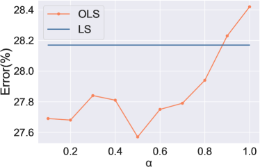
(a) Impact of $\alpha$

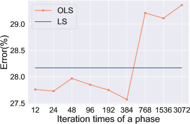
(b) Impact of the updating period

Figure 7: Impact of hyper-parameters. The Top-1 Error of different $\alpha$ and updating period.

Moreover, we also conduct experiments to study the impact of the updating period for the soft label matrix $S$ in the training process. In the previous experiments in Sec. V-A, we set the updating period to one epoch. As shown in Fig. 7(b), we evaluate our approach with different updating periods ( iteration times $\in\{12,24,48,\cdots,1536,3072\}$). The best performance is obtained when the updating period is set to one epoch. We observe that the classification performance is very close when the updating period is less than one epoch (1 epoch is approximately 384 iterations). However, when the updating period is longer than one training epoch, the performance decreases sharply. We analyze that with the training of the network, the predictions become better and better. When using more iterations to update soft labels, the relationships indicated by the early predictions will be very different from that of late ones. The early predictions become out of date for current training.

Importance of relationships among categories. We argue that classification models can benefit from soft labels that contain the knowledge of relationships among different categories. Specifically, we utilize a human uncertainty dataset [72] called CIFAR-10H to verify the reliability of the relationships among different categories. CIFAR-10H captures the full distribution of the labels by collecting votes from more than 50 people for each sample in the CIFAR-10 test set. The human uncertainty labels can be regarded as a kind of soft label that considers the similarities among different categories. They find that models trained on the human uncertainty labels will have better accuracy and generalization than those trained on hard labels. To explore the rationality of relationships among categories found by our approach, we use KL divergence to measure the difference between the predicted probability distribution of the model and the human uncertainty distribution on CIFAR-10H.

TABLE XII: Multiple evaluation results of the model. We first train ResNet-29 with different methods on CIFAR-10. We use the average KL divergence to measure the difference between the prediction distribution of the models and human uncertainty on CIFAR-10H test set.

Method	CIFAR-10 Top-1 Err(%)	CIFAR-10H KL Divergence
Hard Label	7.18	0.2974
Bootsoft [11]	6.91	0.3247
Boothard [11]	7.73	0.3188
Symmetric Cross Entropy [49]	8.66	0.5563
LS [10]	6.81	0.1866
OLS	6.46	0.1399

For a fair comparison, we only consider the correctly predicted samples by each model, when computing the KL Divergence on CIFAR-10H. As shown in Table XII, we list the average KL divergence of different methods on CIFAR-10H [72] and Top-1 Error(%) on CIFAR-10. The results show that the prediction distribution of the model trained by our method is closer to that of humans. Also, this indicates that the model trained by our approach finds more reasonable and correct relationships among categories.

Sample-level soft labels. To verify the effectiveness of the statistical characteristics of accumulating model predictions, we use the predicted distribution of a single sample (denoted as OLS-Single for short) to regularize the training process. To be specific, for each training sample, we randomly select another training sample with the same category. We then acquire the randomly selected training sample’s predictive distribution and utilize this distribution as the soft label to serve as supervision for the current training sample. Based on the ResNet-56, OLS ($25.24\pm 0.18$) outperforms OLS-Single ($26.18\pm 0.30$) by about 1%. This result demonstrates that the accumulation of the predictions from different samples can well explore the relationships among categories.

Calibration effect. The confidence calibration is proposed in [80], which is used to measure the degree of overfitting of the model to the training set. We use the Expected Calibration Error (ECE) [80] to measure the calibration ability of OLS. In Tab. XI, we report the Top-1 Error(%) and ECE on several models, which denotes our method can calibrate neural networks. Experimental results show that our method achieves a lower Top-1 Error than LS by an average of 1.14%. Meanwhile, our method also achieves lower ECE values on three different depth models. This indicates that the proposed method can more effectively prevent over-confident predictions and show better calibration capability.

VI Conclusion

In this paper, we propose an online label smoothing method. We utilize the statistics of the intermediate model predictions to generate soft labels, which are subsequently used to supervise the model. Our soft labels considering the relationships among categories are effective in preventing the overfitting problem of DNNs to the training set. We evaluate our OLS on CIFAR, ImageNet and four fine-grained datasets, respectively. On CIFAR-100, ResNeXt-2x64d trained with our OLS achieves 18.81% Top-1 Error, which brings an 2.11% performance gain. On ImageNet dataset, our OLS brings 1.4% and 1.02% performance gains to ResNet-50 and ResNet-101, respectively. On four fine-grained datasets, OLS outperforms the hard label by 2% in terms of Top-1 Error.

References

- [1] K. Simonyan and A. Zisserman, “Very deep convolutional networks for large-scale image recognition,” in Int. Conf. Learn. Represent., 2015.
- [2] K. He, X. Zhang, S. Ren, and J. Sun, “Deep residual learning for image recognition,” in IEEE Conf. Comput. Vis. Pattern Recog., 2016, pp. 770–778.
- [3] G. Huang, Z. Liu, L. Van Der Maaten, and K. Q. Weinberger, “Densely connected convolutional networks,” in IEEE Conf. Comput. Vis. Pattern Recog., 2017, pp. 4700–4708.
- [4] S. Xie, R. Girshick, P. Dollár, Z. Tu, and K. He, “Aggregated residual transformations for deep neural networks,” in IEEE Conf. Comput. Vis. Pattern Recog., 2017, pp. 1492–1500.
- [5] J. Hu, L. Shen, and G. Sun, “Squeeze-and-excitation networks,” in IEEE Conf. Comput. Vis. Pattern Recog., 2018, pp. 7132–7141.
- [6] M. Sandler, A. G. Howard, M. Zhu, A. Zhmoginov, and L. Chen, “Mobilenetv2: Inverted residuals and linear bottlenecks,” in IEEE Conf. Comput. Vis. Pattern Recog., 2018, pp. 4510–4520.
- [7] S.-H. Gao, M.-M. Cheng, K. Zhao, X.-Y. Zhang, M.-H. Yang, and P. Torr, “Res2net: A new multi-scale backbone architecture,” IEEE Trans. Pattern Anal. Mach. Intell., vol. 43, no. 2, pp. 652–662, 2020.
- [8] A. Krizhevsky and G. Hinton, “Learning multiple layers of features from tiny images,” University of Toronto, Toronto, Ontario, Tech. Rep. 0, 2009.
- [9] J. Deng, W. Dong, R. Socher, L.-J. Li, K. Li, and L. Fei-Fei, “Imagenet: A large-scale hierarchical image database,” in IEEE Conf. Comput. Vis. Pattern Recog., 2009, pp. 248–255.
- [10] C. Szegedy, V. Vanhoucke, S. Ioffe, J. Shlens, and Z. Wojna, “Rethinking the inception architecture for computer vision,” in IEEE Conf. Comput. Vis. Pattern Recog., 2016, pp. 2818–2826.
- [11] S. E. Reed, H. Lee, D. Anguelov, C. Szegedy, D. Erhan, and A. Rabinovich, “Training deep neural networks on noisy labels with bootstrapping,” in Int. Conf. Learn. Represent. Worksh., 2015.
- [12] T. DeVries and G. W. Taylor, “Improved regularization of convolutional neural networks with cutout,” arXiv preprint arXiv:1708.04552, 2017.
- [13] H. Zhang, M. Cisse, Y. N. Dauphin, and D. Lopez-Paz, “mixup: Beyond empirical risk minimization,” in Int. Conf. Learn. Represent., 2018.
- [14] G. Ghiasi, T.-Y. Lin, and Q. V. Le, “Dropblock: A regularization method for convolutional networks,” in Adv. Neural Inform. Process. Syst., 2018, pp. 10 727–10 737.
- [15] Y. Yamada, M. Iwamura, T. Akiba, and K. Kise, “Shakedrop regularization for deep residual learning,” IEEE Access, pp. 186 126–186 136, 2019.
- [16] G.-J. Qi, “Loss-sensitive generative adversarial networks on lipschitz densities,” Int. J. Comput. Vis., vol. 128, no. 5, pp. 1118–1140, 2020.
- [17] G. Hinton, O. Vinyals, and J. Dean, “Distilling the knowledge in a neural network,” in Adv. Neural Inform. Process. Syst. Worksh., 2015.
- [18] M.-E. Nilsback and A. Zisserman, “Automated flower classification over a large number of classes,” in 2008 Sixth Indian Conference on Computer Vision, Graphics & Image Processing, 2008, pp. 722–729.
- [19] C. Wah, S. Branson, P. Welinder, P. Perona, and S. Belongie, “The Caltech-UCSD Birds-200-2011 Dataset,” California Institute of Technology, Tech. Rep. CNS-TR-2011-001, 2011.
- [20] J. Krause, M. Stark, J. Deng, and L. Fei-Fei, “3d object representations for fine-grained categorization,” in Int. Conf. Comput. Vis. Worksh., 2013, pp. 554–561.
- [21] S. Maji, J. Kannala, E. Rahtu, M. Blaschko, and A. Vedaldi, “A database for fine-grained aircraft recognition,” in IEEE Conf. Comput. Vis. Pattern Recog. Worksh., June 2013.
- [22] M. Tan and Q. V. Le, “Efficientnet: Rethinking model scaling for convolutional neural networks,” in Int. Conf. Mech. Learn., vol. 97, 2019, pp. 6105–6114.
- [23] H. Zhao, J. Jia, and V. Koltun, “Exploring self-attention for image recognition,” in IEEE Conf. Comput. Vis. Pattern Recog., 2020, pp. 10 076–10 085.
- [24] L. Zhang, J. Song, A. Gao, J. Chen, C. Bao, and K. Ma, “Be your own teacher: Improve the performance of convolutional neural networks via self distillation,” in Int. Conf. Comput. Vis., 2019, pp. 3712–3721.
- [25] T.-B. Xu and C.-L. Liu, “Data-distortion guided self-distillation for deep neural networks,” in AAAI Conf. Artif. Intell., 2019, pp. 5565–5572.
- [26] L. Xie, J. Wang, Z. Wei, M. Wang, and Q. Tian, “Disturblabel: Regularizing cnn on the loss layer,” in IEEE Conf. Comput. Vis. Pattern Recog., 2016, pp. 4753–4762.
- [27] A. Dubey, O. Gupta, P. Guo, R. Raskar, R. Farrell, and N. Naik, “Pairwise confusion for fine-grained visual classification,” in Eur. Conf. Comput. Vis., 2018, pp. 70–86.
- [28] C. Li, C. Liu, L. Duan, P. Gao, and K. Zheng, “Reconstruction regularized deep metric learning for multi-label image classification,” IEEE Trans. Neural Netw. Learn Syst., vol. 31, no. 7, pp. 2294–2303, 2020.
- [29] L. Zhang, G.-J. Qi, L. Wang, and J. Luo, “Aet vs. aed: Unsupervised representation learning by auto-encoding transformations rather than data,” in IEEE Conf. Comput. Vis. Pattern Recog., 2019, pp. 2547–2555.
- [30] G.-J. Qi, L. Zhang, F. Lin, and X. Wang, “Learning generalized transformation equivariant representations via autoencoding transformations,” IEEE Trans. Pattern Anal. Mach. Intell., 2020.
- [31] G.-J. Qi, L. Zhang, C. W. Chen, and Q. Tian, “Avt: Unsupervised learning of transformation equivariant representations by autoencoding variational transformations,” in Int. Conf. Comput. Vis., 2019, pp. 8130–8139.
- [32] X. Wang, D. Kihara, J. Luo, and G.-J. Qi, “Enaet: A self-trained framework for semi-supervised and supervised learning with ensemble transformations,” IEEE Trans. Image Process., 2020.
- [33] N. Passalis and A. Tefas, “Unsupervised knowledge transfer using similarity embeddings,” IEEE Trans. Neural Netw. Learn Syst., vol. 30, no. 3, pp. 946–950, 2019.
- [34] T. Furlanello, Z. C. Lipton, M. Tschannen, L. Itti, and A. Anandkumar, “Born-again neural networks,” in Int. Conf. Mech. Learn., 2018, pp. 1602–1611.
- [35] S. Ge, Z. Luo, C. Zhang, Y. Hua, and D. Tao, “Distilling channels for efficient deep tracking,” IEEE Trans. Image Process., vol. 29, pp. 2610–2621, 2020.
- [36] N. Wang, W. Zhou, Y. Song, C. Ma, and H. Li, “Real-time correlation tracking via joint model compression and transfer,” IEEE Trans. Image Process., vol. 29, pp. 6123–6135, 2020.
- [37] S. Ge, S. Zhao, C. Li, and J. Li, “Low-resolution face recognition in the wild via selective knowledge distillation,” IEEE Trans. Image Process., vol. 28, no. 4, pp. 2051–2062, 2019.
- [38] Z. Peng, Z. Li, J. Zhang, Y. Li, G.-J. Qi, and J. Tang, “Few-shot image recognition with knowledge transfer,” in Int. Conf. Comput. Vis., 2019, pp. 441–449.
- [39] J. Yao, J. Wang, I. W. Tsang, Y. Zhang, J. Sun, C. Zhang, and R. Zhang, “Deep learning from noisy image labels with quality embedding,” IEEE Trans. Image Process., vol. 28, no. 4, pp. 1909–1922, 2019.
- [40] J. S. Duncan and T. Birkholzer, “Reinforcement of linear structure using parametrized relaxation labeling,” IEEE Trans. Pattern Anal. Mach. Intell., vol. 14, no. 5, pp. 502–515, 1992.
- [41] R. Wang, T. Liu, and D. Tao, “Multiclass learning with partially corrupted labels,” IEEE Trans. Neural Netw. Learn Syst., vol. 29, no. 6, pp. 2568–2580, 2018.
- [42] Y. Wei, C. Gong, S. Chen, T. Liu, J. Yang, and D. Tao, “Harnessing side information for classification under label noise,” IEEE Trans. Neural Netw. Learn Syst., vol. 31, no. 9, pp. 3178–3192, 2020.
- [43] B. Han, I. W. Tsang, L. Chen, C. P. Yu, and S. Fung, “Progressive stochastic learning for noisy labels,” IEEE Trans. Neural Netw. Learn Syst., vol. 29, no. 10, pp. 5136–5148, 2018.
- [44] D. Tanaka, D. Ikami, T. Yamasaki, and K. Aizawa, “Joint optimization framework for learning with noisy labels,” in IEEE Conf. Comput. Vis. Pattern Recog., 2018, pp. 5552–5560.
- [45] J. Han, P. Luo, and X. Wang, “Deep self-learning from noisy labels,” in Int. Conf. Comput. Vis., 2019, pp. 5138–5147.
- [46] M. Ren, W. Zeng, B. Yang, and R. Urtasun, “Learning to reweight examples for robust deep learning,” in Int. Conf. Mech. Learn., 2018, pp. 4334–4343.
- [47] J. Shu, Q. Xie, L. Yi, Q. Zhao, S. Zhou, Z. Xu, and D. Meng, “Meta-weight-net: Learning an explicit mapping for sample weighting,” in Adv. Neural Inform. Process. Syst., 2019, pp. 1919–1930.
- [48] T. Liu and D. Tao, “Classification with noisy labels by importance reweighting,” IEEE Trans. Pattern Anal. Mach. Intell., vol. 38, no. 3, pp. 447–461, 2015.
- [49] Y. Wang, X. Ma, Z. Chen, Y. Luo, J. Yi, and J. Bailey, “Symmetric cross entropy for robust learning with noisy labels,” in Int. Conf. Comput. Vis., 2019, pp. 322–330.
- [50] R. Tanno, A. Saeedi, S. Sankaranarayanan, D. C. Alexander, and N. Silberman, “Learning from noisy labels by regularized estimation of annotator confusion,” in IEEE Conf. Comput. Vis. Pattern Recog., 2019, pp. 11 236–11 245.
- [51] E. Arazo, D. Ortego, P. Albert, N. O’Connor, and K. Mcguinness, “Unsupervised label noise modeling and loss correction,” in Int. Conf. Mech. Learn., 2019, pp. 312–321.
- [52] J. Zhang, V. S. Sheng, T. Li, and X. Wu, “Improving crowdsourced label quality using noise correction,” IEEE Trans. Neural Netw. Learn Syst., vol. 29, no. 5, pp. 1675–1688, 2018.
- [53] M. Fang, T. Zhou, J. Yin, Y. Wang, and D. Tao, “Data subset selection with imperfect multiple labels,” IEEE Trans. Neural Netw. Learn Syst., vol. 30, no. 7, pp. 2212–2221, 2019.
- [54] K. Yi and J. Wu, “Probabilistic end-to-end noise correction for learning with noisy labels,” in IEEE Conf. Comput. Vis. Pattern Recog., 2019, pp. 7017–7025.
- [55] R. Müller, S. Kornblith, and G. E. Hinton, “When does label smoothing help?” in Adv. Neural Inform. Process. Syst., 2019, pp. 4696–4705.
- [56] L. v. d. Maaten and G. Hinton, “Visualizing data using t-sne,” Journal of machine learning research, pp. 2579–2605, 2008.
- [57] L. Yuan, F. E. Tay, G. Li, T. Wang, and J. Feng, “Revisiting knowledge distillation via label smoothing regularization,” in IEEE Conf. Comput. Vis. Pattern Recog., 2020, pp. 3903–3911.
- [58] A. Paszke, S. Gross, S. Chintala, G. Chanan, E. Yang, Z. DeVito, Z. Lin, A. Desmaison, L. Antiga, and A. Lerer, “Automatic differentiation in pytorch,” in Adv. Neural Inform. Process. Syst. Worksh., 2017.
- [59] S.-M. Hu, D. Liang, G.-Y. Yang, G.-W. Yang, and W.-Y. Zhou, “Jittor: a novel deep learning framework with meta-operators and unified graph execution,” Science China Information Sciences, vol. 63, no. 12, pp. 1–21, 2020.
- [60] A. Iscen, G. Tolias, P. Gosselin, and H. Jégou, “A comparison of dense region detectors for image search and fine-grained classification,” IEEE Trans. Image Process., vol. 24, no. 8, pp. 2369–2381, 2015.
- [61] C. Zhang, C. Liang, L. Li, J. Liu, Q. Huang, and Q. Tian, “Fine-grained image classification via low-rank sparse coding with general and class-specific codebooks,” IEEE Trans. Neural Netw. Learn Syst., vol. 28, no. 7, pp. 1550–1559, 2017.
- [62] Y. Zhang, X. Wei, J. Wu, J. Cai, J. Lu, V. Nguyen, and M. N. Do, “Weakly supervised fine-grained categorization with part-based image representation,” IEEE Trans. Image Process., vol. 25, no. 4, pp. 1713–1725, 2016.
- [63] W. Shi, Y. Gong, X. Tao, D. Cheng, and N. Zheng, “Fine-grained image classification using modified dcnns trained by cascaded softmax and generalized large-margin losses,” IEEE Trans. Neural Netw. Learn Syst., vol. 30, no. 3, pp. 683–694, 2019.
- [64] X. Shu, J. Tang, G.-J. Qi, Z. Li, Y.-G. Jiang, and S. Yan, “Image classification with tailored fine-grained dictionaries,” IEEE Trans. Circuit Syst. Video Technol., vol. 28, no. 2, pp. 454–467, 2016.
- [65] Y. Peng, X. He, and J. Zhao, “Object-part attention model for fine-grained image classification,” IEEE Trans. Image Process., vol. 27, no. 3, pp. 1487–1500, 2018.
- [66] H. Zheng, J. Fu, Z. Zha, J. Luo, and T. Mei, “Learning rich part hierarchies with progressive attention networks for fine-grained image recognition,” IEEE Trans. Image Process., vol. 29, pp. 476–488, 2020.
- [67] T. Lin, A. RoyChowdhury, and S. Maji, “Bilinear convolutional neural networks for fine-grained visual recognition,” IEEE Trans. Pattern Anal. Mach. Intell., vol. 40, no. 6, pp. 1309–1322, 2018.
- [68] T. Xiao, T. Xia, Y. Yang, C. Huang, and X. Wang, “Learning from massive noisy labeled data for image classification,” in IEEE Conf. Comput. Vis. Pattern Recog., 2015, pp. 2691–2699.
- [69] C. Zhang, S. Bengio, M. Hardt, B. Recht, and O. Vinyals, “Understanding deep learning requires rethinking generalization,” in Int. Conf. Learn. Represent., 2017.
- [70] I. J. Goodfellow, J. Shlens, and C. Szegedy, “Explaining and harnessing adversarial examples,” in Int. Conf. Learn. Represent., 2015.
- [71] A. Kurakin, I. J. Goodfellow, and S. Bengio, “Adversarial machine learning at scale,” in Int. Conf. Learn. Represent., 2017.
- [72] J. C. Peterson, R. M. Battleday, T. L. Griffiths, and O. Russakovsky, “Human uncertainty makes classification more robust,” in Int. Conf. Comput. Vis., 2019, pp. 9616–9625.
- [73] J. Redmon, S. Divvala, R. Girshick, and A. Farhadi, “You only look once: Unified, real-time object detection,” in IEEE Conf. Comput. Vis. Pattern Recog., 2016, pp. 779–788.
- [74] F. Fang, L. Li, H. Zhu, and J. Lim, “Combining faster r-cnn and model-driven clustering for elongated object detection,” IEEE Trans. Image Process., vol. 29, pp. 2052–2065, 2020.
- [75] F. Sun, T. Kong, W. Huang, C. Tan, B. Fang, and H. Liu, “Feature pyramid reconfiguration with consistent loss for object detection,” IEEE Trans. Image Process., vol. 28, no. 10, pp. 5041–5051, 2019.
- [76] S. Ren, K. He, R. Girshick, and J. Sun, “Faster r-cnn: Towards real-time object detection with region proposal networks,” IEEE Trans. Pattern Anal. Mach. Intell., vol. 39, no. 6, pp. 1137–1149, 2017.
- [77] W. Liu, D. Anguelov, D. Erhan, C. Szegedy, S. Reed, C.-Y. Fu, and A. C. Berg, “Ssd: Single shot multibox detector,” in Eur. Conf. Comput. Vis., 2016, pp. 21–37.
- [78] Z. Tian, C. Shen, H. Chen, and T. He, “Fcos: Fully convolutional one-stage object detection,” in Int. Conf. Comput. Vis., 2019, pp. 9627–9636.
- [79] M. Everingham, L. Van Gool, C. K. Williams, J. Winn, and A. Zisserman, “The pascal visual object classes (voc) challenge,” Int. J. Comput. Vis., vol. 88, no. 2, pp. 303–338, 2010.
- [80] C. Guo, G. Pleiss, Y. Sun, and K. Q. Weinberger, “On calibration of modern neural networks,” in Int. Conf. Mech. Learn., 2017, pp. 1321–1330.