Elliptical Symmetry Tests in R

Abstract

The assumption of elliptical symmetry has an important role in many theoretical developments and applications, hence it is of primary importance to be able to test whether that assumption actually holds true or not. Various tests have been proposed in the literature for this problem. To the best of our knowledge, none of them has been implemented in R. The focus of this paper is the implementation of several well-known tests for elliptical symmetry together with some recent tests. We demonstrate the testing procedures with a real data example.

Key words: Elliptical symmetry, Hypothesis testing, Skew distributions, Skewness

MSC2010 subject classification: 62-04

1 Introduction

Let $\mathbf{X}_{1},\ldots,\mathbf{X}_{n}$ denote a sample of $n$ i.i.d. $d$-dimensional observations. A $d$-dimensional random vector $\mathbf{X}$ is said to be elliptically symmetric about some location parameter $\boldsymbol{\theta}\in\mathbb{R}^{d}$ if its density $\underline{f}$ is of the form

$$\mathbf{x}\mapsto{\underline{f}(\mathbf{x};\boldsymbol{\theta},\boldsymbol{\Sigma},f)}=c_{d,f}|\boldsymbol{\Sigma}|^{-1/2}f\left(\|\boldsymbol{\Sigma}^{-1/2}(\mathbf{x}-\boldsymbol{\theta})\|\right),\qquad\mathbf{x}\in\mathbb{R}^{d},$$ (1)

where $\boldsymbol{\Sigma}\in\mathcal{S}_{d}$ (the class of symmetric positive definite real $d\times d$ matrices) is a scatter parameter, $f:\mathbb{R}^{+}_{0}\to\mathbb{R}^{+}$ is an a.e.  strictly positive function called radial density, and $c_{d,f}$ is a normalizing constant depending on $f$ and the dimension $d$. Many well-known and widely used multivariate distributions are elliptical. The multivariate normal, multivariate Student $t$, multivariate power-exponential, symmetric multivariate stable, symmetric multivariate Laplace, multivariate logistic, multivariate Cauchy, and multivariate symmetric general hyperbolic distribution are all examples of elliptical distributions. The family of elliptical distributions has several appealing properties. For instance, it has a simple stochastic representation, clear parameter interpretation, it is closed under affine transformations, and its marginal and conditional distributions are also elliptically symmetric: see Paindaveine, (2014) for details. Thanks to its mathematical tractability and nice properties, it became a fundamental assumption in multivariate analysis and many applications. Numerous statistical procedures therefore rest on the assumption of elliptical symmetry: one- and $K$-sample location and shape problems (Um and Randles,, 1998; Hallin and Paindaveine,, 2002, 2006; Hallin et al.,, 2006), serial dependence and time series (Hallin and Paindaveine,, 2004), one- and $K$-sample principal component problems (Hallin et al.,, 2010, 2014), multivariate tail estimation (Dominicy et al.,, 2017), to cite but a few. Elliptical densities are also considered in portfolio theory (Owen and Rabinovitch,, 1983), capital asset pricing models (Hodgson et al.,, 2002), semiparametric density estimation (Liebscher,, 2005), graphical models (Vogel and Fried,, 2011), and many other areas.

Given the omnipresence of the assumption of elliptical symmetry, it is essential to be able to test whether that assumption actually holds true or not for the data at hand. Numerous tests have been proposed in the literature, including Beran, (1979), Baringhaus, (1991), Koltchinskii and Sakhanenko, (2000), Manzotti et al., (2002), Schott, (2002), Huffer and Park, (2007), Cassart, (2007) and Babić et al., (2021). Tests for elliptical symmetry based on Monte Carlo simulations can be found in Diks and Tong, (1999) and Zhu and Neuhaus, (2000); Li et al., (1997) recur to graphical methods and Zhu and Neuhaus, (2004) build conditional tests. We refer the reader to Serfling, (2006) and Sakhanenko, (2008) for extensive reviews and performance comparisons. To the best of our knowledge, none of these tests is available in the open software R. The focus of this paper is to close this gap by implementing several well-known tests for elliptical symmetry together with some recent tests. The test of Beran, (1979) is neither distribution-free nor affine-invariant; moreover, there are no practical guidelines to the choice of the basis functions involved in the test statistic. Therefore, we opt not to include it in the package. Baringhaus, (1991) proposes a Cramér-von Mises type test for spherical symmetry based on the independence between norm and direction. Dyckerhoff et al., (2015) have shown by simulations that this test can be used as a test for elliptical symmetry in dimension 2. This test assumes the location parameter to be known and its asymptotic distribution is not simple to use (plus no proven validity in dimensions higher than 2), hence we decided not to include it in the package. Thus, the tests suggested by Koltchinskii and Sakhanenko, (2000), Manzotti et al., (2002), Schott, (2002), Huffer and Park, (2007), Cassart, (2007) and Babić et al., (2021) are implemented in the package ellipticalsymmetry.

This paper describes the tests for elliptical symmetry that have been implemented in the ellipticalsymmetry package, together with a detailed description of the functions that are available in the package. The use of the implemented functions is illustrated using financial data.

2 Testing for elliptical symmetry

In this section, we focus on tests for elliptical symmetry that have been implemented in our new ellipticalsymmetry package. Besides formal definitions of test statistics and limiting distributions, we also explain the details on computing.

2.1 Test by Koltchinskii and Sakhanenko

Koltchinskii and Sakhanenko, (2000) develop a class of omnibus bootstrap tests for unspecified location that are affine invariant and consistent against any fixed alternative. The estimators of the unknown parameters are as follows: $\hat{\boldsymbol{\theta}}=n^{-1}\sum_{i=1}^{n}\mathbf{X}_{i}$ and $\hat{\boldsymbol{\Sigma}}=n^{-1}\sum_{i=1}^{n}(\mathbf{X}_{i}-\hat{\boldsymbol{\theta}})(\mathbf{X}_{i}-\hat{\boldsymbol{\theta}})^{\prime}$. Define $\mathbf{Y}_{i}=\hat{\boldsymbol{\Sigma}}^{-1/2}(\mathbf{X}_{i}-\hat{\boldsymbol{\theta}})$ and let $\mathcal{F}_{B}$ be a class of Borel functions from $\mathbb{R}^{d}$ to $\mathbb{R}$. Their test statistics are functionals (for example, sup-norms) of the stochastic process

$$n^{-1/2}\sum_{i=1}^{n}\left(f(\mathbf{Y}_{i})-m_{f}(||\mathbf{Y}_{i}||)\right),\vspace{-1mm}$$

where $f\in\mathcal{F}_{B}$ and $m_{f}(\rho)$ is the average value of $f$ on the sphere with radius $\rho>0$. Several examples of classes $\mathcal{F}_{B}$ and test statistics based on the sup-norm of the above process are considered in Koltchinskii and Sakhanenko, (2000). Here, we restrict our attention to $\mathcal{F}_{B}:=\left\{I_{0<||\mathbf{x}||\leq t}\psi\left(\frac{\mathbf{x}}{||\mathbf{x}||}\right):\psi\in G_{l},||\psi||_{2}\leq 1,t>0\right\}$ where $I_{A}$ stands for the indicator function of $A$, $G_{l}$ for the linear space of spherical harmonics of degree less than or equal to $l$ in $\mathbb{R}^{d}$, and $||\cdot||_{2}$ is the $L^{2}$-norm on the unit sphere $\mathcal{S}^{d-1}$ in $\mathbb{R}^{d}$. With these quantities in hand, the test statistic becomes

$$Q_{{KS}}^{(n)}:=n^{-1/2}\max_{1\leq j\leq n}\left(\sum_{s=1}^{\text{dim}(G_{l})}\left(\sum_{k=1}^{j}\psi_{s}\left(\frac{\mathbf{Y}_{[k]}}{||\mathbf{Y}_{[k]}||}\right)-\delta_{s1}\right)^{2}\right)^{1/2},$$

where $\mathbf{Y}_{[i]}$ denotes the $i$th order statistic from the sample $\mathbf{Y}_{1},\dots,\mathbf{Y}_{n}$ ordered according to their $L^{2}$-norm, $\{\psi_{s},\ s=1,\dots,\,\text{dim}(G_{l})\}$ denotes an orthonormal basis of $G_{l},\ \psi_{1}=1$, and $\delta_{ij}=1$ for $i=j$ and $0$ otherwise. The test statistic is relatively simple to construct if we have formulas for spherical harmonics. In dimension $2$ spherical harmonics coincide with sines and cosines on the unit circle. The detailed construction of the test statistic $Q_{{KS}}^{(n)}$ for dimensions $2$ and $3$ can be found in Sakhanenko, (2008). In order to be able to use $Q_{{KS}}^{(n)}$ in higher dimensions, we need corresponding formulas for spherical harmonics. Using recursive formulas from Müller, (1966) and equations given in Manzotti and Quiroz, (2001) we obtained spherical harmonics of degree one to four in arbitrary dimension. The reader should bare in mind that larger degree leads to better power performance of this test. A drawback of this test is that it requires bootstrap procedures to obtain critical values.

In our R package, this test can be run using a function called KoltchinskiiSakhanenko(). The syntax for this function is very simple:

    KoltchinskiiSakhanenko(X, R=1000, nJobs = -1),

where X is an input to this function consisting of a data set which must be a matrix and R stands for the number of bootstrap replicates. The default number of replicates is set to $1000$. The nJobs argument represents the number of CPU cores to use for the calculation. This is a purely technical option which is used to speed up the computation of bootstrap based tests. The default value $-1$ indicates that all cores except one are used.

2.2 The MPQ test

Manzotti et al., (2002) develop a test based on spherical harmonics. The estimators of the unknown parameters are the sample mean denoted as $\hat{\boldsymbol{\theta}}$ and the unbiased sample covariance matrix given by $\hat{\boldsymbol{\Sigma}}=\frac{1}{n-1}\sum_{i=1}^{n}(\mathbf{X}_{i}-\hat{\boldsymbol{\theta}})(\mathbf{X}_{i}-\hat{\boldsymbol{\theta}})^{\prime}$. Define again $\mathbf{Y}_{i}=\hat{\boldsymbol{\Sigma}}^{-1/2}(\mathbf{X}_{i}-\hat{\boldsymbol{\theta}})$. When the $\mathbf{X}_{i}^{\prime}s$ are elliptically symmetric, then $\mathbf{Y}_{i}/||\mathbf{Y}_{i}||$ should be uniformly distributed on the unit sphere, and Manzotti et al., (2002) chose this property as the basis of their test. The uniformity of the standardized vectors $\mathbf{Y}_{i}/||\mathbf{Y}_{i}||$ can be checked in different ways. Manzotti et al., (2002) opt to verify this uniformity using spherical harmonics. For a fixed $\varepsilon>0$, let $\rho_{n}$ be the $\varepsilon$ sample quantile of $||\mathbf{Y}_{1}||,\dots,||\mathbf{Y}_{n}||$. Then, the test statistic is

$$Q_{{MPQ}}^{(n)}=n\mathop{\scalebox{2.0}{$\sum$}}_{h\in\mathcal{S}_{jl}}\bigg{(}\frac{1}{n}\mathop{\scalebox{2.0}{$\sum$}}_{i=1}^{n}h\bigg{(}\frac{\mathbf{Y}_{i}}{||\mathbf{Y}_{i}||}\bigg{)}I(||\mathbf{Y}_{i}||>\rho_{n})\bigg{)}^{2}$$

for $l\geq j\geq 3$, where $\mathcal{S}_{jl}=\bigcup_{j\leq i\leq l}\mathcal{H}_{i}$ and $\mathcal{H}_{i}$ is the set of spherical harmonics of degree $i$. In the implementation of this test we used spherical harmonics of degree $3$ and $4$. The asymptotic distribution of the test statistic $Q_{{MPQ}}^{(n)}$ is $(1-\varepsilon)\chi$, where $\chi$ is a variable with a chi-squared distribution with $\nu_{jl}$ degrees of freedom, where $\nu_{jl}$ denotes the total number of functions in $\mathcal{S}_{jl}$. Note that $Q_{{MPQ}}^{(n)}$ is only a necessary condition statistic for the null hypothesis of elliptical symmetry and therefore this test does not have asymptotic power against all alternatives. In the ellipticalsymmetry package, this test is implemented as the MPQ function with the following syntax

    MPQ(X, epsilon = 0.05)

As before, X is a numeric matrix that represents the data while epsilon is an option that allows the user to indicate the proportion of points $\mathbf{Y}_{i}$ close to the origin which will not be used in the calculation. By doing this, extra assumptions on the radial density in (1) are avoided. The default value of epsilon is set to 0.05.

2.3 Schott’s test

Schott, (2002) develops a Wald-type test for elliptical symmetry based on the analysis of covariance matrices. The test compares the sample fourth moments with the expected theoretical ones under ellipticity. Given that the test statistic involves consistent estimates of the covariance matrix of the sample fourth moments, the existence of eight-order moments is required. Furthermore, the test has very low power against several alternatives. The final test statistic is of a simple form, even though it requires lengthy notations.

For an elliptical distribution with mean $\boldsymbol{\theta}$ and covariance matrix $\boldsymbol{\Sigma}$, the fourth moment defined as ${\boldsymbol{M}_{4}}=E\{(\mathbf{X}-\boldsymbol{\theta})(\mathbf{X}-\boldsymbol{\theta})^{\prime}\otimes(\mathbf{X}-\boldsymbol{\theta})(\mathbf{X}-\boldsymbol{\theta})^{\prime}\}$, with $\otimes$ the Kronecker product, has the form

$${\boldsymbol{M}_{4}}=(1+\kappa)((\mathbf{I}_{d^{2}}+K_{dd})(\boldsymbol{\Sigma}\otimes\boldsymbol{\Sigma})+vec(\boldsymbol{\Sigma})vec(\boldsymbol{\Sigma})^{\prime})$$ (2)

where $K_{dd}$ is a commutation matrix (Magnus,, 1988), $\mathbf{I}_{d}$ is the $d\times d$ identity matrix, and $\kappa$ is a scalar which can be expressed using the characteristic function of the elliptical distribution. Here the $vec$ operator stacks all components of a $d\times d$ matrix $\boldsymbol{M}$ on top of each other to yield the $d^{2}$ vector ${\rm vec}(\boldsymbol{M})$. Let $\hat{\boldsymbol{\Sigma}}$ denote the usual unbiased sample covariance matrix and $\hat{\boldsymbol{\theta}}$ the sample mean. A simple estimator of ${\boldsymbol{M}_{4}}$ is given by $\hat{\boldsymbol{M}}_{4}=\frac{1}{n}\sum_{i=1}^{n}(\mathbf{X}_{i}-\hat{\boldsymbol{\theta}})(\mathbf{X}_{i}-\hat{\boldsymbol{\theta}})^{\prime}\otimes(\mathbf{X}_{i}-\hat{\boldsymbol{\theta}})(\mathbf{X}_{i}-\hat{\boldsymbol{\theta}})^{\prime}$ and its standardized version is given by

$${\hat{\boldsymbol{M}}_{4*}}=(\hat{\boldsymbol{\Sigma}}^{-1/2^{\prime}}\otimes\hat{\boldsymbol{\Sigma}}^{-1/2^{\prime}}){\hat{\boldsymbol{M}}_{4}}(\hat{\boldsymbol{\Sigma}}^{-1/2}\otimes\hat{\boldsymbol{\Sigma}}^{-1/2}).$$

Then, an estimator of $vec({\boldsymbol{M}}_{4})$ is constructed as ${\boldsymbol{G}}=vec({\boldsymbol{N}}_{4})vec({\boldsymbol{N}}_{4})^{\prime}vec(\hat{\boldsymbol{M}}_{4*})/(3d(d+2))$, and it is consistent if and only if ${\boldsymbol{M}}_{4}$ is of the form (2); here ${\boldsymbol{N}}_{4}$ represents the value of ${\boldsymbol{M}}_{4}$ under the multivariate standard normal distribution. Note that the asymptotic mean of $\boldsymbol{v}=n^{1/2}(vec(\hat{\boldsymbol{M}}_{4*})-{\boldsymbol{G}})$ is $0$ if and only if (2) holds and this expression is used to construct the test statistic. Denote the estimate of the asymptotic covariance matrix of $n^{1/2}\boldsymbol{v}$ as $\hat{\boldsymbol{\Phi}}$. The Wald test statistic is then formalized as $T=\boldsymbol{v}^{\prime}\hat{\boldsymbol{\Phi}}^{-}\boldsymbol{v}$, where $\hat{\boldsymbol{\Phi}}^{-}$ is a generalized inverse of $\hat{\boldsymbol{\Phi}}$. For more technical details we refer the reader to Section 2 in Schott, (2002). In order to define Schott’s test statistic, we further have to define the following quantities:

$$(1+\hat{\kappa})=\frac{1}{nd(d+2)}\sum_{i=1}^{n}\{(\mathbf{X}_{i}-\hat{\boldsymbol{\theta}})^{\prime}\hat{\boldsymbol{\Sigma}}^{-1}(\mathbf{X}_{i}-\hat{\boldsymbol{\theta}})\}^{2}$$

$$(1+\hat{\eta})=\frac{1}{nd(d+2)(d+4)}\sum_{i=1}^{n}\{(\mathbf{X}_{i}-\hat{\boldsymbol{\theta}})^{\prime}\hat{\boldsymbol{\Sigma}}^{-1}(\mathbf{X}_{i}-\hat{\boldsymbol{\theta}})\}^{3}$$

$$(1+\hat{\omega})=\frac{1}{nd(d+2)(d+4)(d+6)}\sum_{i=1}^{n}\{(\mathbf{X}_{i}-\hat{\boldsymbol{\theta}})^{\prime}\hat{\boldsymbol{\Sigma}}^{-1}(\mathbf{X}_{i}-\hat{\boldsymbol{\theta}})\}^{4}.$$

Moreover, let $\hat{\beta}_{1}=(1+\hat{\omega})^{-1}/24,\enspace\hat{\beta}_{2}=-3a\{24(1+\hat{\omega})^{2}+12(d+4)a(1+\hat{\omega})\}^{-1}$, $a=(1+\hat{\omega})+(1+\hat{\kappa})^{3}-2(1+\hat{\kappa})(1+\hat{\eta})$. Finally, the test statistic becomes

$$T=n\left[\hat{\beta}_{1}\text{tr}(\hat{\boldsymbol{M}}_{4*}^{2})+\hat{\beta}_{2}\text{vec}(\mathbf{I}_{d})^{\prime}\hat{\boldsymbol{M}}_{4*}^{2}\text{vec}(\mathbf{I}_{d})-\{3\hat{\beta}_{1}+(d+2)\hat{\beta}_{2}\}d(d+2)(1+\hat{\kappa})^{2}\right].$$

It has an asymptotic chi-squared distribution with degrees of freedom $\displaystyle\nu_{d}=d^{2}+\frac{d(d-1)(d^{2}+7d-6)}{24}-1.$

The Schott test can be performed in our package by using the function Schott with the very simple syntax Schott(X), where X is a numeric matrix of data values.

2.4 Test by Huffer and Park

Huffer and Park, (2007) propose a Pearson chi-square type test with multi-dimensional cells. Under the null hypothesis of ellipticity the cells have asymptotically equal expected cell counts and after determining the observed cell counts, the test statistic is easily computed. Let $\hat{\boldsymbol{\theta}}$ be the sample mean and $\hat{\boldsymbol{\Sigma}}=n^{-1}\sum_{i=1}^{n}(\mathbf{X}_{i}-\hat{\boldsymbol{\theta}})(\mathbf{X}_{i}-\hat{\boldsymbol{\theta}})^{\prime}$ the sample covariance matrix. Define $\mathbf{Y}_{i}=\mathbf{R}(\mathbf{X}_{i}-\hat{\boldsymbol{\theta}}),$ where the matrix $\mathbf{R}=\mathbf{R}(\hat{\boldsymbol{\Sigma}})$ is a function of $\hat{\boldsymbol{\Sigma}}$ such that $\mathbf{R}\hat{\boldsymbol{\Sigma}}\mathbf{R}=\mathbf{I}_{d}$. Typically $\mathbf{R}=\hat{\boldsymbol{\Sigma}}^{-1/2}$ as for the previous tests. However, Huffer and Park suggest to use the Gram-Schmidt transformation because that will lead to standardized data whose joint distribution does not depend on $\boldsymbol{\theta}$ or $\boldsymbol{\Sigma}$. In order to compute the test statistic, the space $\mathbb{R}^{d}$ should be divided into $c$ spherical shells centered at the origin such that each shell contains an equal number of the scaled residuals $\mathbf{Y}_{i}$. The next step is to divide $\mathbb{R}^{d}$ into $g$ sectors such that for any pair of sectors there is an orthogonal transformation mapping one onto the other. Therefore, the $c$ shells and $g$ sectors divide $\mathbb{R}^{d}$ into $gc$ cells which, under elliptical symmetry, should contain $n/(gc)$ of the vectors $\mathbf{Y}_{i}$. The test statistic then has the simple form

$$HP_{n}=\sum_{\pi}(U_{\pi}-np)^{2}/(np),$$

where $U_{\pi}$ are cell counts for $\pi=(i,j)$ with $1\leq i\leq g$ and $1\leq j\leq c$ and $p=1/(gc)$.

In the R package we are considering three particular ways to partition the space: using (i) the $2^{d}$ orthants, (ii) permutation matrices and (iii) a cyclic group consisting of rotations by angles which are multiples of $2\pi/g$. The first two options can be used for any dimension, while the angles are supported only for dimension 2. Huffer and Park’s test can be run using a function called HufferPark. The syntax, including all options, for the function HufferPark is for instance

HufferPark(X, c, R = NA, sector = "orthants", g = NA, nJobs = -1).

We will now provide a detailed description of its arguments. X is an input to this function consisting of a data set. sector is an option that allows the user to specify the type of sectors used to divide the space. Currently supported options are "orthants", "permutations" and "bivariateangles", the last one being available only in dimension $2$. The g argument indicates the number of sectors. The user has to choose g only if sector = "bivariateangles" and it denotes the number of regions used to divide the plane. In this case, regions consist of points whose angle in polar coordinates is between $2(m-1)\pi/g$ and $2m\pi/g$ for $m\in\{1\dots g\}$. If sector is set to "orthants", then g is fixed and equal to $2^{d}$, while for sector = "permutations" g is $d!$. No matter what type of sectors is chosen, the user has to specify the number of spherical shells that are used to divide the space, which is c. The value of c should be such that the average cell counts $\displaystyle n/(gc)$ are not too small. Several settings with different sample size, and different values of $g$ and $c$ can be found in the simulation studies presented in Sections 4 and 5 of Huffer and Park, (2007). As before, nJobs represents the number of CPU cores to use for the calculation. The default value -1 indicates that all cores except one are used.

The asymptotic distribution is available only under sector = "orthants" when the underlying distribution is close to normal. It is a linear combination of chi-squared random variables and it depends on eigenvalues of congruent sectors used to divide the space $\mathbb{R}^{d}$. Otherwise, bootstrap procedures are required and the user can freely choose the number of bootstrap replicates, denoted as R. Note that by default sector is set to "orthants" and R = NA.

2.5 Pseudo-Gaussian test

Cassart, (2007) and Cassart et al., (2008) construct Pseudo-Gaussian tests for specified and unspecified location that are most efficient against a multivariate form of Fechner-type asymmetry (defined in Cassart, (2007), Chapter 3). These tests are based on Le Cam’s asymptotic theory of statistical experiments. We start by describing the specified-location Pseudo-Gaussian test. The unknown parameter $\boldsymbol{\Sigma}$ is estimated by using Tyler, (1987)’s estimator of scatter which we simply denote by $\hat{\boldsymbol{\Sigma}}$. Let $m_{k}(\boldsymbol{\theta},\boldsymbol{\Sigma}):=n^{-1}\sum_{i=1}^{n}(\|\boldsymbol{\Sigma}^{-1/2}(\mathbf{X}_{i}-\boldsymbol{\theta})\|)^{k}$, $U_{i}(\boldsymbol{\theta},\boldsymbol{\Sigma}):=\frac{\boldsymbol{\Sigma}^{-1/2}(\mathbf{X}_{i}-\boldsymbol{\theta})}{\|\boldsymbol{\Sigma}^{-1/2}(\mathbf{X}_{i}-\boldsymbol{\theta})\|}$ and

$$\mathbf{S}^{\mathbf{U}}_{i}(\boldsymbol{\theta},\boldsymbol{\Sigma}):=((\mathbf{U}_{i1}(\boldsymbol{\theta},\boldsymbol{\Sigma}))^{2}\text{sign} (\mathbf{U}_{i1}(\boldsymbol{\theta},\boldsymbol{\Sigma})),\dots,(\mathbf{U}_{id}(\boldsymbol{\theta},\boldsymbol{\Sigma}))^{2}\text{sign}(\mathbf{U}_{id}(\boldsymbol{\theta},\boldsymbol{\Sigma})))^{\prime}.\vspace{-1mm}$$

The test statistic then has the simple form

$$Q_{{p{\cal G},\boldsymbol{\theta}}}^{(n)}=\frac{d(d+2)}{3n{m_{4}}(\boldsymbol{\theta},\hat{}\boldsymbol{\Sigma})}\sum_{i,j=1}^{n}(\|\hat{}\boldsymbol{\Sigma}^{-1/2}(\mathbf{X}_{i}-\boldsymbol{\theta})\|)^{2}(\|\hat{}\boldsymbol{\Sigma}^{-1/2}(\mathbf{X}_{j}-\boldsymbol{\theta})\|)^{2}\mathbf{S}^{\prime\mathbf{U}}_{i}(\boldsymbol{\theta},\hat{}\boldsymbol{\Sigma})\mathbf{S}^{\mathbf{U}}_{j}(\boldsymbol{\theta},\hat{}\boldsymbol{\Sigma})\vspace{-1mm}$$

and follows asymptotically a chi-squared distribution $\chi^{2}_{d}$ with $d$ degrees of freedom. Finite moments of order four are required.

In most cases the assumption of a specified center is however unrealistic. Cassart, (2007) therefore proposes also a test for the scenario when location is not specified. The estimator of the unknown $\boldsymbol{\theta}$ is the sample mean denoted by $\hat{\boldsymbol{\theta}}$. Let $\mathbf{Y}_{i}=\hat{}\boldsymbol{\Sigma}^{-1/2}(\mathbf{X}_{i}-\hat{}\boldsymbol{\theta})$. The test statistic takes on the guise

$$Q_{{p{\cal G}}}^{(n)}:=(\boldsymbol{\Delta}_{{{\cal G}}}(\hat{}\boldsymbol{\theta},\hat{}\boldsymbol{\Sigma}))^{\prime}(\boldsymbol{\Gamma}_{{{\cal G}}}(\hat{}\boldsymbol{\theta},\hat{}\boldsymbol{\Sigma}))^{-1}\boldsymbol{\Delta}_{{{\cal G}}}(\hat{}\boldsymbol{\theta},\hat{}\boldsymbol{\Sigma}),$$

where

$$\boldsymbol{\Delta}_{{{\cal G}}}(\hat{}\boldsymbol{\theta},\hat{}\boldsymbol{\Sigma})=n^{-1/2}\sum_{i=1}^{n}\|\mathbf{Y}_{i}\|\left(c_{d}(d+1)m_{1}(\hat{}\boldsymbol{\theta},\hat{}\boldsymbol{\Sigma})\mathbf{U}_{i}(\hat{}\boldsymbol{\theta},\hat{}\boldsymbol{\Sigma})-\|\mathbf{Y}_{i}\|\mathbf{S}^{\mathbf{U}}_{i}(\hat{}\boldsymbol{\theta},\hat{}\boldsymbol{\Sigma})\right)$$

and

$$\boldsymbol{\Gamma}_{{{\cal G}}}(\hat{}\boldsymbol{\theta},\hat{}\boldsymbol{\Sigma}):=$$

$$\left(\frac{3}{d(d+2)}m_{4}(\hat{}\boldsymbol{\theta},\hat{}\boldsymbol{\Sigma})-2c_{d}^{2}(d+1)m_{1}(\hat{}\boldsymbol{\theta},\hat{}\boldsymbol{\Sigma})m_{3}(\hat{}\boldsymbol{\theta},\hat{}\boldsymbol{\Sigma})+c_{d}^{2}\frac{(d+1)^{2}}{d}(m_{1}(\hat{}\boldsymbol{\theta},\hat{}\boldsymbol{\Sigma}))^{2}m_{2}(\hat{}\boldsymbol{\theta},\hat{}\boldsymbol{\Sigma})\right)\mathbf{I}_{d}$$

with $c_{d}=4\Gamma(d/2)/((d^{2}-1)\sqrt{\pi}\Gamma(\frac{d-1}{2}))$, $\Gamma(\cdot)$ being the Gamma function. The test rejects the null hypothesis of elliptical symmetry at asymptotic level $\alpha$ whenever the test statistic $Q_{{p{\cal G}}}^{(n)}$ exceeds $\chi^{2}_{d;1-\alpha}$, the upper $\alpha$-quantile of a $\chi^{2}_{d}$ distribution. We refer to Chapter 3 of Cassart, (2007) for formal details.

This test can be run in our package by calling the function pseudoGaussian with the simple syntax

   pseudoGaussian(X, location = NA).

Besides X which is a numeric matrix of data values, now we have an extra argument location which allows the user to specify the known location. The default is set to NA which means that the unspecified location test will be performed unless the user specifies location.

2.6 SkewOptimal test

Recently, Babić et al., (2021) proposed a new test for elliptical symmetry both for specified and unspecified location. These tests are based on Le Cam’s asymptotic theory of statistical experiments and are optimal against generalized skew-elliptical alternatives (defined in Section 2 of said paper) but they remain quite powerful under a much broader class of non-elliptical distributions.

The test statistic for the specified location scenario has a very simple form and an asymptotic chi-squared distribution. The test rejects the null hypothesis whenever $Q_{\boldsymbol{\theta}}^{(n)}=n(\bar{\mathbf{X}}-\boldsymbol{\theta})^{\prime}\hat{}\boldsymbol{\Sigma}^{-1}(\bar{\mathbf{X}}-\boldsymbol{\theta})$ exceeds the $\alpha$-upper quantile $\chi^{2}_{d;1-\alpha}$. Here, $\hat{\boldsymbol{\Sigma}}$ is Tyler, (1987)’s estimator of scatter and $\bar{\boldsymbol{X}}$ is the sample mean.

When the location is not specified, Babić et al., (2021) propose tests that have a simple asymptotic chi-squared distribution under the null hypothesis of ellipticity, are affine-invariant, computationally fast, have a simple and intuitive form, only require finite moments of order 2, and offer much flexibility in the choice of the radial density $f$ at which optimality (in the maximin sense) is achieved. Note that the Gaussian $f$ is excluded, though, due to a singular information matrix; see Babić et al., (2021). We implemented in our package the test statistic based on the radial density $f$ of the multivariate $t$ distribution, multivariate power-exponential and multivariate logistic, though in principle any non-Gaussian choice for $f$ is possible. The test requires lengthy notations, but its implementation is straightforward. For the sake of generality, we will derive the test statistic for a general (but fixed) $f$, and later on provide the expressions of $f$ for the three special cases implemented in our package. Let $\varphi_{f}(x)=-\frac{f^{\prime}(x)}{f(x)}$ and $\mathbf{Y}_{i}=\hat{}\boldsymbol{\Sigma}^{-1/2}(\mathbf{X}_{i}-\hat{}\boldsymbol{\theta})$ where $\hat{}\boldsymbol{\theta}$ is the sample mean. In order to construct the test statistic, we first have to define the quantities

$$\displaystyle{\boldsymbol{\Delta}}_{f}(\hat{}\boldsymbol{\theta},\hat{}\boldsymbol{\Sigma})=2n^{-1/2}\dot{\Pi}(0)\sum_{i=1}^{n}\left[\|\mathbf{Y}_{i}\|-\frac{d}{\widehat{\mathcal{K}}_{d,f}(\hat{}\boldsymbol{\theta},\hat{}\boldsymbol{\Sigma})}\varphi_{f}(\|\mathbf{Y}_{i}\|)\right]\frac{\mathbf{Y}_{i}}{\|\mathbf{Y}_{i}\|}$$

and

$$\widehat{\boldsymbol{\Gamma}}_{f}(\hat{}\boldsymbol{\theta},\hat{}\boldsymbol{\Sigma}):=\frac{{4(\dot{\Pi}(0))^{2}}}{nd}\sum_{i=1}^{n}\left[\|\mathbf{Y}_{i}\|-\frac{d}{\widehat{\mathcal{K}}_{d,f}(\hat{}\boldsymbol{\theta},\hat{}\boldsymbol{\Sigma})}\varphi_{f}(\|\mathbf{Y}_{i}\|)\right]^{2}\mathbf{I}_{d}$$

where $\widehat{\mathcal{K}}_{d,f}(\hat{}\boldsymbol{\theta},\hat{}\boldsymbol{\Sigma}):=\frac{1}{n}\sum_{i=1}^{n}\left[\displaystyle\varphi_{f}^{\prime}(\|\mathbf{Y}_{i}\|)+\frac{d-1}{\|\mathbf{Y}_{i}\|}\varphi_{f}(\|\mathbf{Y}_{i}\|)\right]$ and $\Pi$ is the cdf of the standard normal distribution (we use $\dot{\Pi}(\cdot)$ for the derivative). Finally, the test statistic is of the form $Q^{(n)}_{f}:=({\boldsymbol{\Delta}}_{f}(\hat{}\boldsymbol{\theta},\hat{}\boldsymbol{\Sigma}))^{\prime}(\widehat{\boldsymbol{\Gamma}}_{f}(\hat{}\boldsymbol{\theta},\hat{}\boldsymbol{\Sigma}))^{-1}{\boldsymbol{\Delta}}_{f}(\hat{}\boldsymbol{\theta},\hat{}\boldsymbol{\Sigma})$ and it has a chi-squared distribution with $d$ degrees of freedom. The test is valid under the entire semiparametric hypothesis of elliptical symmetry with unspecified center and uniformly optimal against any type of generalized skew-$f$ alternative.

From this general expression, one can readily derive the test statistics for specific choices of $f$. In our case, the radial density of the multivariate Student $t$ distribution corresponds to $f(x)=(1+\frac{1}{\nu}x^{2})^{-(\nu+d)^{2}}$, where $\nu\in(0,\infty)$ represents the degrees of freedom, while that of the multivariate logistic distribution is given by $\displaystyle f(x)=\frac{\exp{(-x^{2})}}{[1+\exp{(-x^{2}})]^{2}}$ and of the multivariate power-exponential by $\displaystyle f(x)=\exp{\left(-\frac{1}{2}x^{2\beta}\right)}$, where $\beta\in(0,\infty)$ is a parameter related to kurtosis.

These tests can be run in R using a function called SkewOptimal with the syntax

   SkewOptimal(X, location = NA, f = "t", param = NA)

Depending on the type of the test some of the input arguments are not required. X and location are the only input arguments for the specified location test, and have the same role as for the Pseudo-Gaussian test. As before, the default value for location is set to NA which implies that the unspecified location test will be performed unless the user specifies location. For the unspecified location test, besides the data matrix X, the input arguments are f and param. The f argument is a string that specifies the type of the radial density based on which the test is built. Currently supported options are "t", "logistic" and "powerExp". Note that the default is set to "t". The role of the param argument is as follows. If f = "t" then param denotes the degrees of freedom of the multivariate $t$ distribution. Given that the default radial density is "t", it follows that the default value of param represents the degrees of freedom of the multivariate $t$ distribution and it is set to $4$. Note also that the degrees of freedom have to be greater than $2$. If f = "powerExp" then param denotes the kurtosis parameter $\beta$, in which case the value of param has to be different from $1$ because $\beta=1$ corresponds to the multivariate normal distribution. The default value is set to $0.5$.

2.7 Time complexity

We conclude the description of tests for elliptical symmetry by comparing their time complexity in terms of the big O notation (Cormen et al.,, 2009). More concretely, we are comparing the number of simple operations that are required to evaluate the test statistics and the p-values. Table 1 summarizes the time complexity of the implemented tests.

The test of Koltchinskii and Sakhanenko is computationally more demanding than the bootstrap version of the test of Huffer and Park. Among unspecified location tests that do not require bootstrap procedures, the most computationally expensive test is the MPQ test under the realistic assumption that $n>d$. Regarding the specified location tests we can conclude that the Pseudo-Gaussian test is more computationally demanding than the SkewOptimal test. Note that both the test of Koltchinskii and Sakhanenko and the MPQ test are based on spherical harmonics up to degree $4$. In case we would use spherical harmonics of higher degrees, the tests would of course become even more computationally demanding.

We have seen that several tests require bootstrap procedures and therefore are by default computationally demanding. Such tests require the calculation of the statistic on the resampled data $R$ times in order to get the p-value, where $R$ is the number of bootstrap replicates. Consequently, the time required to obtain the p-value in such cases is $R$ times the time to calculate the test statistic. For the tests that do not involve bootstrap procedures, the p-value is calculated using the inverse of the cdf of the asymptotic distribution under the null hypothesis, which is considered as one simple operation. The exception here is the test of Huffer and Park whose asymptotic distribution is more complicated and includes $O(c)$ operations where $c$ is an integer and represents an input parameter for this test.

Table 1: Time complexity of the various tests for elliptical symmetry

	statistics	p-value
KoltchinskiiSakhanenko	$O(n\log n+nd^{5})$	$O(Rn\log n+Rnd^{5})$
MPQ	$O(n\log n+nd^{5})$	$O(1)$
Schott	$O(nd^{2}+d^{6})$	$O(1)$
HufferPark	$O(nd^{2}+d^{3})$	$O(c)$
HufferPark (bootstrap)	$O(nd^{2}+d^{3})$	$O(Rnd^{2}+Rd^{3})$
PseudoGaussian (specified location)	$O(n^{2}d+nd^{2}+d^{3})$	$O(1)$
PseudoGaussian	$O(nd^{2}+d^{3})$	$O(1)$
SkewOptimal (specified location)	$O(nd+d^{3})$	$O(1)$
SkewOptimal	$O(nd^{2}+d^{3})$	$O(1)$

3 Illustrations using financial data

Mean-Variance analysis was introduced by Markowitz, (1952) as a model for portfolio selection. In this model, the portfolio risk expressed through the historical volatility is minimized for a given expected return, or the expected return is maximized given the risk. The model is widely used for making portfolio decisions, primarily because it can be easily optimized using quadratic programming techniques. However, the model has some shortcomings among which the very important one that it does not consider the prior wealth of the investor that makes decisions. This prior wealth is important since it influences the satisfaction that an investor has from gains. For example, the gain of 50$ will not bring the same satisfaction to someone whose wealth is 1$ as to someone whose wealth is 1000$. This satisfaction further affects the decision-making process in portfolio selection. Because of that and other financial reasons, a more general concept of expected utility maximization is used (see e.g. Schoemaker, (2013)). However, the expected utility maximization is not an easy optimization problem, and some additional assumptions must be made in order to solve it. Hence, despite the expected utility maximization being more general, the mean-variance approach is still used due to its computational simplicity. Chamberlain, (1983) showed that the two approaches coincide if the returns are elliptically distributed. In other words, under elliptical symmetry the mean-variance optimization solves the expected utility maximization for any increasing concave utility function. Therefore, we want to test if the assumption of elliptical symmetry holds or not for financial return data. The data set that we analyze contains daily stock log returns of $3$ major equity market indexes from North America: S&P 500 (US), TSX (Canada) and IPC (Mexico). The sample consists of 5369 observations, from January 2000 through July 2020. To remove temporal dependencies by filtering, following the suggestion of Lombardi and Veredas, (2009), GARCH(1,1) time series models were fitted to each series of log-returns.

We test if the returns are elliptically symmetric in different time periods using a rolling window analysis. The window has a size of one year and it is rolled every month, i.e. we start with the window January 2000 - December 2000 and we test for elliptical symmetry. Then we shift the starting point by one month, that is we consider February 2000 - January 2001 and we test again for elliptical symmetry. We keep doing this until the last possible window. The following tests are used for every window: the test by Koltchinskii and Sakhanenko with R = 100 bootstrap replicates, the MPQ test, Schott’s test, the bootstrap test by Huffer and Park based on orthants with c = 3 and with the number of bootstrap replicates R = 100, the Pseudo-Gaussian test and the SkewOptimal test with the default values of the parameters. For every window we calculate the p-value. The results are presented in Figure  1, where the horizontal line present on every plot indicates the 0.05 significance level.

Even though all these tests address the null hypothesis of elliptical symmetry, they have different powers for different alternative distributions and some tests may fail to detect certain departures from the null hypothesis. Certain tests are also by nature more conservative than others. We refer the reader to Babić et al., (2021) for a comparative simulation study that includes the majority of the tests available in this package. This diversity in behavior presents nice opportunities. For instance, when all tests agree, we can be pretty sure about the nature of the analyzed data. One could also combine the six tests into a multiple testing setting by using a Bonferroni correction, though this is not what we are doing here.

The following general conclusions can be drawn from Figure  1.

• In the past 20 years, the return data do not follow the elliptical distribution at least half of time. In other words, there are many periods between 2000 and 2020 where the data exhibit some form of skewness or other type of symmetry, invalidating thus the mean-variance analysis.

• The broader periods where the hypothesis of elliptical symmetry cannot be rejected are 2000-2004, 2005-2006, 2012-2013, 2015-2017 (for Schott’s test only 2015-2016). In these periods, the tests may have only occasional rejections without a longer time period of rejections.

• In the period around the financial crisis in 2008, almost all tests reject the null hypothesis of ellipticity. This clearly shows that, in the periods of crisis, the assumption of elliptical symmetry is less likely to hold.

Figure 1: North America indexes (S&P, TSX and IPC)

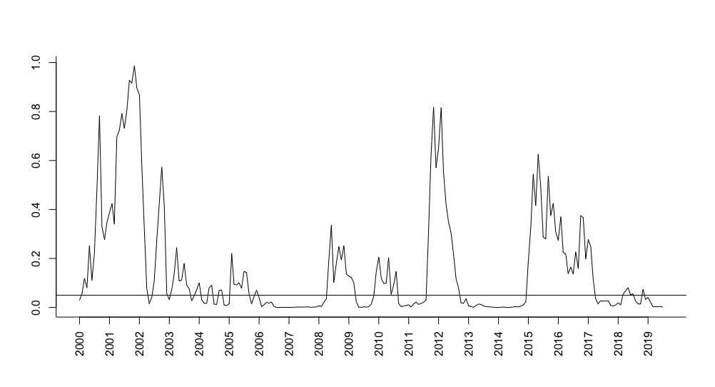
(a) SkewOptimal

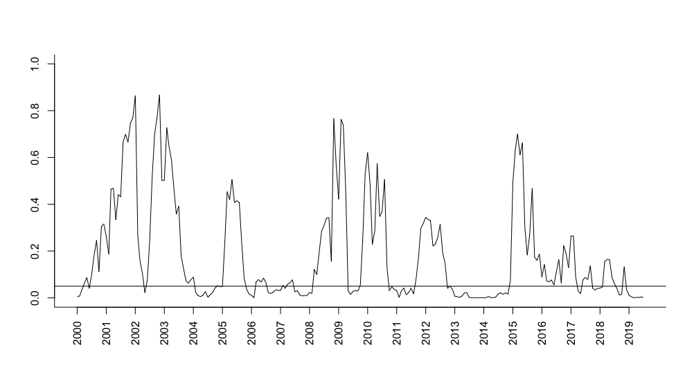
(b) Pseudo-Gaussian

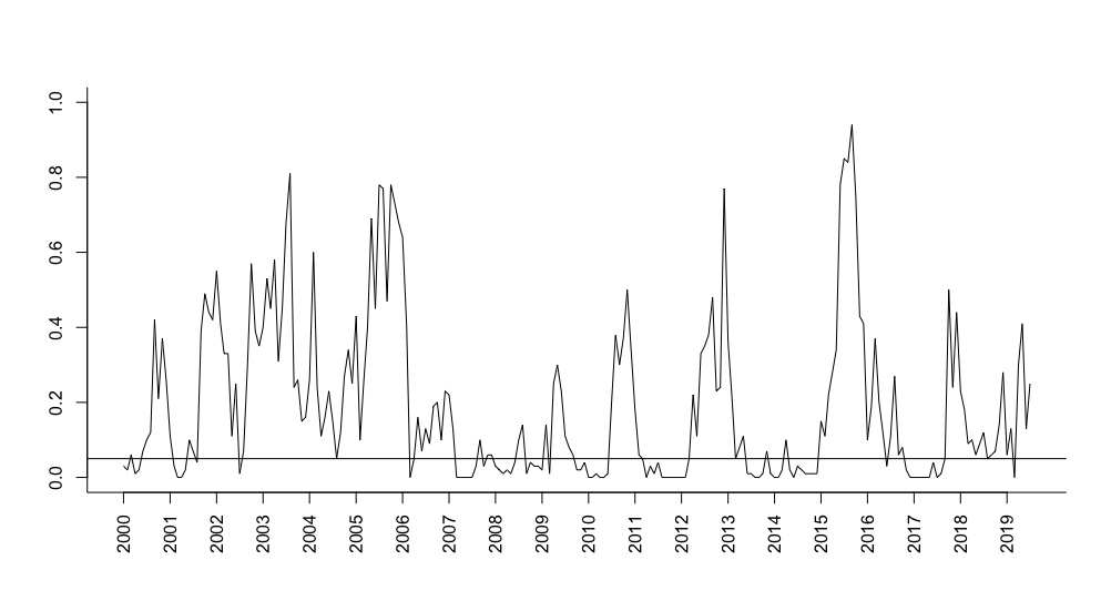
(c) KoltchinskiiSakhanenko

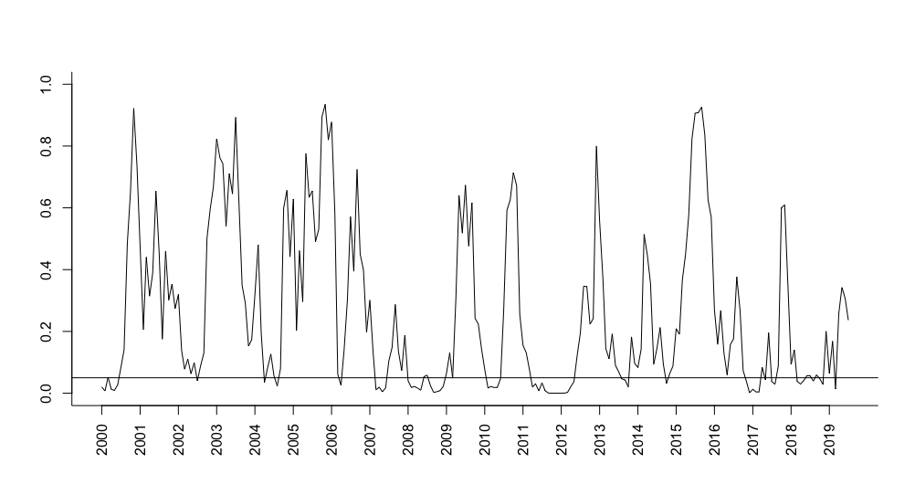
(d) MPQ

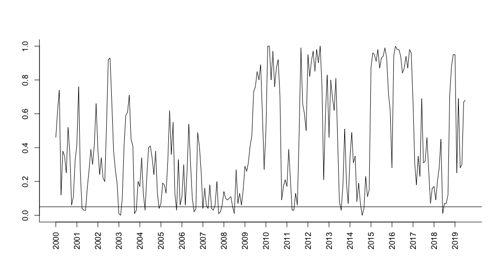
(e) HufferPark

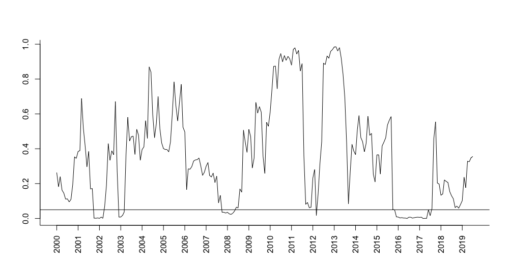
(f) Schott

The plots show the p-values of the corresponding tests for all rolling windows that we considered between 2000 and 2020. The years on the x-axis mark the rolling windows for which the starting point is January of that year. The horizontal line present on every plot indicates the 0.05 significance level.

With the aim of guiding the reader through the functions that are available in the ellipticalsymmetry package, we now focus on the window January 2008 - December 2008. We start with the test by Koltchinskii and Sakhanenko.

> KoltchinskiiSakhanenko(data2008, R = 100)

Test for elliptical symmetry by Koltchinskii and Sakhanenko

data:  data2008
statistic =  6.0884, p-value = 0.02
alternative hypothesis: the distribution is not elliptically symmetric

The KoltchinskiiSakhanenko output is simple and clear. It reports the value of the test statistic and p-value. For this particular data set the test statistic is equal to $6.0884$ and the p-value is $0.02$. Note that here we specify the number of bootstrap replicates to be R = 100.

The MPQ test and Schott’s test can be performed by running very simple commands:

> MPQ(data2008)

Test for elliptical symmetry by Manzotti et al.

data:  data2008
statistic = 25.737, p-value = 0.04047
alternative hypothesis: the distribution is not elliptically symmetric

> Schott(data2008)

¯Schott test for elliptical symmetry

data:  data2008
statistic = 24.925, p-value = 0.03532
alternative hypothesis: the distribution is not elliptically symmetric

Given the number of the input arguments, the function for the test by Huffer and Park deserves some further comments. The non-bootstrap version of the test can be performed by running the command

> HufferPark(data2008, c = 3)

Test for elliptical symmetry by Huffer and Park

data:  data2008
statistic = 24.168, p-value = 0.109
alternative hypothesis: the distribution is not elliptically symmetric

By specifying R the bootstrap will be applied:

> HufferPark(data2008, c= 3, R = 100)

The p-value for the bootstrap version of the test is equal to $0.11$. Note that in both cases we used the default value for sector, that is "orthants".

¯Test for elliptical symmetry by Huffer and Park

data:  data2008
statistic = 24.168, p-value = 0.11
alternative hypothesis: the distribution is not elliptically symmetric

If we want to change the type of sectors used to divide the space, we can do it by running the command

HufferPark(data2008, c=3, R = 100, sector = "permutations")

This version yields a p-value equal to $0.16$.

Another very easy-to-use test is the Pseudo-Gaussian test:

> PseudoGaussian(data2008)

¯Pseudo-Gaussian test for elliptical symmetry

data:  data2008
statistic = 9.486, p-value = 0.02348
alternative hypothesis: the distribution is not elliptically symmetric

Eventually, the following simple command will run the SkewOptimal test based on the radial density of the multivariate $t$ distribution with $4$ degrees of freedom (note that the degrees of freedom could be readily changed by specifying the param argument).

> SkewOptimal(data2008)

 SkewOptimal test for elliptical symmetry

data:  data2008
statistic = 12.209, p-value = 0.006701
alternative hypothesis: the distribution is not elliptically symmetric

The test based on the radial density of the multivariate logistic distribution can be performed by simply adding f = "logistic":

> SkewOptimal(data2008, f = "logistic")

This version of the SkewOptimal test yields a p-value equal to $0.0003484$. Finally, if we want to run the test based on the radial density of the multivariate power-exponential distribution, we have to set f to "powerExp". The kurtosis parameter equal to $0.5$ will be used unless specified otherwise.

> SkewOptimal(data2008, f = "powerExp")

The resulting p-value equals $0.002052$. The kurtosis parameter can be changed by assigning a different value to param. For example,

SkewOptimal(data2008, f = "powerExp", param = 1.2)

We can conclude that the null hypothesis is rejected at the $5\%$ level by all tests except by Huffer and Park’s tests. Luckily the tests available in the package mostly agree. In general, in situations of discordance between two (or more) tests, a practitioner may compare the essence of the tests as described in this paper and check if, perhaps, one test is more suitable for the data at hand than the other (e.g., if assumptions are not met). The freedom of choice among several tests for elliptical symmetry is an additional feature of our new package.

4 Conclusion

In this paper, we have described several existing tests for elliptical symmetry and explained in details their R implementation in our new package ellipticalsymmetry. The implemented functions are simple to use, and we illustrate this via a real data analysis. The availability of several tests for elliptical symmetry is clearly an appealing strength of our new package.

References

- Babić et al., (2021) Babić, S., Gelbgras, L., Hallin, M., and Ley, C. (2021). Optimal tests for elliptical symmetry: specified and unspecified location. Bernoulli, in press.
- Baringhaus, (1991) Baringhaus, L. (1991). Testing for spherical symmetry of a multivariate distribution. The Annals of Statistics, 19:899–917.
- Beran, (1979) Beran, R. (1979). Testing for ellipsoidal symmetry of a multivariate density. The Annals of Statistics, 7:150–162.
- Cassart, (2007) Cassart, D. (2007). Optimal tests for symmetry. PhD thesis, Univ. libre de Bruxelles, Brussels.
- Cassart et al., (2008) Cassart, D., Hallin, M., and Paindaveine, D. (2008). Optimal detection of Fechner-asymmetry. Journal of Statistical Planning and Inference, 138:2499–2525.
- Chamberlain, (1983) Chamberlain, G. (1983). A characterization of the distributions that imply mean—variance utility functions. Journal of Economic Theory, 29(1):185–201.
- Cormen et al., (2009) Cormen, T. H., Leiserson, C. E., Rivest, R. L., and Stein, C. (2009). Introduction to Algorithms. MIT press.
- Diks and Tong, (1999) Diks, C. and Tong, H. (1999). A test for symmetries of multivariate probability distributions. Biometrika, 86:605–614.
- Dominicy et al., (2017) Dominicy, Y., Ilmonen, P., and Veredas, D. (2017). Multivariate Hill estimators. International Statistical Review, 85(1):108–142.
- Dyckerhoff et al., (2015) Dyckerhoff, R., Ley, C., and Paindaveine, D. (2015). Depth-based runs tests for bivariate central symmetry. Annals of the Institute of Statistical Mathematics, 67(5):917–941.
- Hallin et al., (2006) Hallin, M., Oja, H., and Paindaveine, D. (2006). Semiparametrically efficient rank-based inference for shape. II. Optimal r-estimation of shape. The Annals of Statistics, 34(6):2757–2789.
- Hallin and Paindaveine, (2002) Hallin, M. and Paindaveine, D. (2002). Optimal tests for multivariate location based on interdirections and pseudo-Mahalanobis ranks. The Annals of Statistics, 30(4):1103–1133.
- Hallin and Paindaveine, (2004) Hallin, M. and Paindaveine, D. (2004). Rank-based optimal tests of the adequacy of an elliptic VARMA model. Annals of Statistics, 32:2642–2678.
- Hallin and Paindaveine, (2006) Hallin, M. and Paindaveine, D. (2006). Semiparametrically efficient rank-based inference for shape. I. Optimal rank-based tests for sphericity. The Annals of Statistics, 34(6):2707–2756.
- Hallin et al., (2010) Hallin, M., Paindaveine, D., and Verdebout, T. (2010). Optimal rank-based testing for principal components. The Annals of Statistics, 38(6):3245–3299.
- Hallin et al., (2014) Hallin, M., Paindaveine, D., and Verdebout, T. (2014). Efficient R-estimation of principal and common principal components. Journal of the American Statistical Association, 109:1071–1083.
- Hodgson et al., (2002) Hodgson, D. J., Linton, O., and Vorkink, K. (2002). Testing the capital asset pricing model efficiently under elliptical symmetry: A semiparametric approach. Journal of Applied Econometrics, 17(6):617–639.
- Huffer and Park, (2007) Huffer, F. W. and Park, C. (2007). A test for elliptical symmetry. Journal of Multivariate Analysis, 98(2):256–281.