Compatibility of Carnot efficiency with finite power in an underdamped Brownian Carnot cycle in small temperature-difference regime

Abstract

We study the possibility of achieving the Carnot efficiency in a finite-power underdamped Brownian Carnot cycle. Recently, it was reported that the Carnot efficiency is achievable in a general class of finite-power Carnot cycles in the vanishing limit of the relaxation times. Thus, it may be interesting to clarify how the efficiency and power depend on the relaxation times by using a specific model. By evaluating the heat-leakage effect intrinsic in the underdamped dynamics with the instantaneous adiabatic processes, we demonstrate that the compatibility of the Carnot efficiency and finite power is achieved in the vanishing limit of the relaxation times in the small temperature-difference regime. Furthermore, we show that this result is consistent with a trade-off relation between power and efficiency by explicitly deriving the relation of our cycle in terms of the relaxation times.

I Introduction

Heat engines constitute one of the indispensable technologies in our modern society, and much effort has been conducted to improve their performance in various scientific or engineering fields [1]. Heat engines convert supplied heat into output work. Moreover, their ratio can be used as the efficiency to characterize the performance of heat engines. The Carnot cycle is one of the most important models of heat engines, which operates between hot and cold heat baths with constant temperatures $T_{h}$ and $T_{c}$ ($<T_{h}$). Moreover, the cycle is composed of two isothermal processes and two adiabatic processes. Carnot demonstrated that the efficiency of any heat engine is limited by the upper bound called the Carnot efficiency [2]:

$$\eta_{C}\equiv 1-\frac{T_{c}}{T_{h}}.$$ (1)

It is known that we can reach the Carnot efficiency by the reversible cycle, where the heat engine always remains at equilibrium and is typically operated quasistatically, which implies that the engine spends an infinitely long time per cycle. Moreover, power, defined as output work per unit time, is another important quantity for evaluating the performance of heat engines. When we operate the heat engines quasistatically, power vanishes. Thus, several studies have been devoted to investigating the feasibility of finite-power heat engines with Carnot efficiency [3, 4, 5, 4, 6, 7, 8, 9, 10, 11, 12, 13, 14, 15, 16].

However, Shiraishi et al. [17, 18, 19] recently proved a trade-off relation between power $P$ and efficiency $\eta$ in general heat engines described by the Markov process. The trade-off relation is given by

$$P\leq A\eta(\eta_{C}-\eta),$$ (2)

where $A$ is a positive constant depending on the heat engine details. Based on this relation, the power should vanish as the efficiency approaches the Carnot efficiency. Similar trade-off relations to Eq. (2) have been obtained in various heat engine models [20, 21, 22, 23]. In particular, Dechant and Sasa derived a specific expression of $A$ for stochastic heat engines described by the Langevin equation [23].

Recently, Holubec and Ryabov reported that the Carnot efficiency could be obtained in a general class of finite-power Carnot cycles in the vanishing limit of the relaxation times [24]. Although this result seems to contradict the trade-off relation in Eq. (2), they pointed out the possibility that $A$ in Eq. (2) diverges in the vanishing limit of the relaxation times, and the Carnot efficiency and finite power are compatible without breaking the trade-off relation in Eq. (2). Thus, it may be interesting to study how the efficiency and power depend on the relaxation times in more detail by using a specific model.

The Brownian Carnot cycle with instantaneous adiabatic processes and a time-dependent harmonic potential is a simple model, which is easy to analyze and is frequently used to study the efficiency and power [24, 25, 26, 27]. However, it is pointed out that the instantaneous adiabatic process in the overdamped Brownian Carnot cycle inevitably causes a heat leakage [26, 27, 28]. In the overdamped dynamics, the inertial effect of the Brownian particle is disregarded, and the system is only described by its position. Nevertheless, heat leakage is related to the kinetic energy of the particle, as seen below. When the overdamped limit is considered in the underdamped dynamics, the averaged kinetic energy of the Brownian particle is equal to $k_{B}T/2$ in the isothermal process with temperature $T$, where $k_{B}$ is the Boltzmann constant. Then, after the instantaneous adiabatic processes in the above cycle, the kinetic energy relaxes toward the temperature of the subsequent isothermal process, and an additional heat proportional to the temperature difference flows. This heat leakage decreases the efficiency of the cycle. Thus, we must consider the underdamped dynamics to evaluate the effect of the heat leakage on the efficiency and power of the Brownian Carnot cycle with the instantaneous adiabatic processes.

In this paper, we demonstrate that it is possible to achieve the Carnot efficiency in the underdamped finite-power Brownian Carnot cycle by considering the vanishing limit of the relaxation times of both position and velocity in the small temperature-difference regime, where the heat leakage due to the instantaneous adiabatic processes can be negligible. As shown below, $\eta_{C}-\eta$ in Eq. (2) is proportional to the entropy production. We show that the above compatibility is made possible by the diverging constant $A$ in Eq. (2) and the vanishing entropy production, which can be expressed in terms of the two relaxation times of the system.

The rest of this paper is organized as follows. In Sec. II, we introduce the Brownian particle trapped by the harmonic potential and describe it by the underdamped Langevin equation. We also introduce the isothermal process and instantaneous adiabatic process in this section. In Sec. III, we construct the Carnot cycle using the Brownian particle. In Sec. IV, we present the results of numerical simulations of the underdamped Brownian Carnot cycle when we vary the temperature difference and the relaxation times of the system. From these results, we demonstrate that the efficiency of our cycle approaches the Carnot efficiency while maintaining finite power as the relaxation times vanish in the small temperature-difference regime. In Sec. V, we explain the results of the numerical simulations in Sec. IV based on the trade-off relation in Eq. (2). Section VI presents the summary and discussion.

II Model

II.1 Underdamped system

We consider a Brownian particle in the surrounding medium with a temperature $T$. When the particle is trapped in the harmonic potential

$$V(x,t)=\frac{1}{2}\lambda(t)x^{2},$$ (3)

the dynamics of the particle is described by the underdamped Langevin equation

$$\dot{x}= v,$$ (4)

$$m\dot{v}= -\gamma v-\lambda x+\sqrt{2\gamma k_{B}T}\xi,$$ (5)

where, $x$, $v$, and $m$ are the position, velocity, and mass of the particle, respectively. The dot denotes the time derivative or a quantity per unit time. We use $\gamma$ as the constant friction coefficient independent of $T$ and set the Boltzmann constant $k_{B}=1$ for simplicity. The stiffness $\lambda(t)$ of the harmonic potential changes over time. The Gaussian white noise $\xi(t)$ satisfies $\langle\xi(t)\rangle=0$ and $\langle\xi(t)\xi(t^{\prime})\rangle=\delta(t-t^{\prime})$, where $\langle\cdots\rangle$ denotes statistical average. In this system, the relaxation times of the position $\tau_{x}$ and velocity $\tau_{v}$ are defined as follows:

$$\tau_{x}(t)\equiv \frac{\gamma}{\lambda(t)},$$ (6)

$$\tau_{v}\equiv \frac{m}{\gamma},$$ (7)

where $\tau_{x}(t)$ depends on the time through the stiffness $\lambda(t)$. We introduce the distribution function $p(x,v,t)$ to describe the state of the system at time $t$. The time evolution of $p(x,v,t)$ can be described by the Kramers equation [29] corresponding to Eqs. (4) and (5),

$$\begin{split}\frac{\partial}{\partial t}p(x,v,t)=&-\frac{\partial}{\partial x}(vp(x,v,t))\\ &+\frac{\partial}{\partial v}\left[\frac{\gamma}{m}v+\frac{\lambda}{m}x+\frac{\gamma T}{m^{2}}\frac{\partial}{\partial v}\right]p(x,v,t)\\ =&-\frac{\partial}{\partial x}j_{x}(x,v,t)-\frac{\partial}{\partial v}j_{v}(x,v,t),\end{split}$$ (8)

where $j_{x}(x,v,t)$ and $j_{v}(x,v,t)$ are the probability currents defined as follows:

$$j_{x}(x,v,t)\equiv vp(x,v,t),$$ (9)

$$j_{v}(x,v,t)\equiv -\left[\frac{\gamma}{m}v+\frac{\lambda}{m}x+\frac{\gamma T}{m^{2}}\frac{\partial}{\partial v}\right]p(x,v,t).$$ (10)

Here, we define the three variables $\sigma_{x}(t)\equiv\langle x^{2}\rangle$, $\sigma_{v}(t)\equiv\langle v^{2}\rangle$, and $\sigma_{xv}(t)\equiv\langle xv\rangle$. By using Eq. (8), we can derive the following equations:

$$\dot{\sigma}_{x}= 2\sigma_{xv},$$ (11)

$$\dot{\sigma}_{v}= \frac{2\gamma T}{m^{2}}-\frac{2\gamma}{m}\sigma_{v}-\frac{2\lambda}{m}\sigma_{xv},$$ (12)

$$\dot{\sigma}_{xv}= \sigma_{v}-\frac{\lambda}{m}\sigma_{x}-\frac{\gamma}{m}\sigma_{xv}$$ (13)

describing the time evolution of $\sigma_{x}$, $\sigma_{v}$, and $\sigma_{xv}$ [25]. Below, we assume that the probability distribution $p(x,v,t)$ is a Gaussian distribution:

$$\begin{split}p(x,v,t)=&\frac{1}{\sqrt{4\pi^{2}(\sigma_{x}\sigma_{v}-\sigma_{xv}^{2})}}\\ &\times\exp\left\{-\frac{\sigma_{x}v^{2}+\sigma_{v}x^{2}-2\sigma_{xv}xv}{2(\sigma_{x}\sigma_{v}-\sigma_{xv}^{2})}\right\}.\end{split}$$ (14)

Thus, the state of the Brownian particle can only be described by the above three variables. In this model, the internal energy $E(t)$ and entropy $S(t)$ of the Brownian particle are defined as follows:

$$E(t)\equiv \int^{\infty}_{-\infty}dx\int^{\infty}_{-\infty}dv\ p(x,v,t)\ \left[\frac{1}{2}mv^{2}+\frac{1}{2}\lambda(t)x^{2}\right]$$

$$=\frac{1}{2}m\sigma_{v}(t)+\frac{1}{2}\lambda(t)\sigma_{x}(t),$$ (15)

$$S(t)\equiv -\int^{\infty}_{-\infty}dx\int^{\infty}_{-\infty}dv\ p(x,v,t)\ln p(x,v,t)$$

$$= \frac{1}{2}\ln(\sigma_{x}(t)\sigma_{v}(t)-\sigma_{xv}^{2}(t))+\ln(2\pi)+1.$$ (16)

II.2 Isothermal process

We define the heat and work during a time interval $t_{i}<t<t_{f}$ in an isothermal process. In this process, the Brownian particle interacts with the heat bath at a constant temperature $T$. We assume that the stiffness $\lambda(t)$ changes smoothly in this process. The heat flux $\dot{Q}$ flowing from the heat bath to the Brownian particle is defined as the statistical average of the work performed by the force from the heat bath to the Brownian particle (see Chap. 4 of Ref. [30]),

$$\dot{Q}(t)\equiv\left\langle\left(-\gamma v+\sqrt{2\gamma T}\xi(t)\right)\circ v\right\rangle,$$ (17)

where $\circ$ represents the Stratonovich-type product. Using Eqs. (4) and (5), we derive the heat flux $\dot{Q}(t)$ as follows:

$$\dot{Q}(t)=\frac{1}{2}\lambda(t)\dot{\sigma}_{x}(t)+\frac{1}{2}m\dot{\sigma}_{v}(t).$$ (18)

Thus, we obtain the heat $Q$ flowing in this interval as

$$\begin{split}Q=&\int^{t_{f}}_{t_{i}}dt\ \left(\frac{1}{2}\lambda\dot{\sigma}_{x}\right)+\int^{t_{f}}_{t_{i}}dt\ \left(\frac{1}{2}m\dot{\sigma}_{v}\right)\\ =&Q^{o}+\Delta K,\end{split}$$ (19)

where

$$Q^{o}\equiv \int^{t_{f}}_{t_{i}}dt\ \left(\frac{1}{2}\lambda\dot{\sigma}_{x}\right),$$ (20)

$$\Delta K\equiv \frac{1}{2}m\sigma_{v}(t_{f})-\frac{1}{2}m\sigma_{v}(t_{i}).$$ (21)

Here, $Q^{o}$ represents the heat related to the potential change, and $\Delta K$ is the difference between the initial and final (averaged) kinetic energies of the Brownian particle. In the overdamped system [26], $Q^{o}$ is regarded as the heat instead of $Q$ in Eq. (19). However, in the underdamped system under consideration, the heat also includes the kinetic part $\Delta K$.

The output work during this interval is defined as follows:

$$\begin{split}W&\equiv-\int^{t_{f}}_{t_{i}}dt\int^{\infty}_{-\infty}dx\int^{\infty}_{-\infty}dv\ p(x,v,t)\frac{\partial V(x,t)}{\partial t}\\ &=-\frac{1}{2}\int^{t_{f}}_{t_{i}}dt\ \dot{\lambda}\sigma_{x}\\ &=Q-\Delta E,\end{split}$$ (22)

where we used Eqs. (II.1) and (19) for the derivation from the middle to the last equality, and defined $\Delta E\equiv E(t_{f})-E(t_{i})$. The last equality in Eq. (22) represents the first law of thermodynamics.

II.3 Instantaneous adiabatic process

As an adiabatic process connecting the end of the isothermal process with temperature $T_{1}$ to the beginning of the next isothermal process with temperature $T_{2}$, we use instantaneous changes in the potential and heat bath at $t=t_{0}$, which we regard as the final time of the isothermal process with temperature $T_{1}$ [26]. In this process, the stiffness $\lambda(t)$ jumps from $\lambda_{1}$ to $\lambda_{2}$, and we instantaneously switch the temperature of the heat bath from $T_{1}$ to $T_{2}$, maintaining the probability distribution unchanged. Because this process is instantaneous, no heat exchange occurs, and the output work $W^{ad}_{1\to 2}$ is equal to the negative value of the internal energy change $\Delta E^{ad}_{1\to 2}$ due to the first law of thermodynamics as

$$W^{ad}_{1\to 2}=-\Delta E^{ad}_{1\to 2}=-\frac{1}{2}(\lambda_{2}-\lambda_{1})\sigma_{x}(t_{0}).$$ (23)

III Carnot cycle

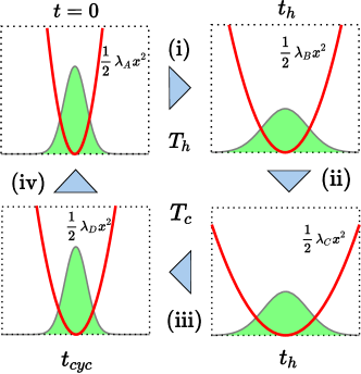
Figure 1: Schematic illustration of the Brownian Carnot cycle. In each box, the bottom horizontal line denotes the position coordinate $x$, and the boundary curve of the green filled area denotes the probability distribution of $x$. The red solid line corresponds to the harmonic potential. This cycle is composed of (i) hot isothermal process, (ii) instantaneous adiabatic process, (iii) cold isothermal process, and (iv) instantaneous adiabatic process.

We construct a Carnot cycle operating between the two heat baths with the temperatures $T_{h}$ and $T_{c}$ (see Fig. 1) by combining the isothermal processes and the instantaneous adiabatic processes introduced in Sec. II.

First, we define a protocol of a finite-time Carnot cycle with stiffness $\lambda(t)$ as follows: The hot isothermal process with temperature $T_{h}$ lasts for $0<t<t_{h}$, and the stiffness $\lambda$ varies from $\lambda_{A}$ to $\lambda_{B}$ [Fig. 1(i)]. In the following instantaneous adiabatic process, we switch the stiffness from $\lambda_{B}$ to $\lambda_{C}$ and the temperature of the heat bath from $T_{h}$ to $T_{c}$ at $t=t_{h}$, [Fig. 1(ii)]. The cold isothermal process with temperature $T_{c}$ lasts for $t_{h}<t<t_{h}+t_{c}$, and the stiffness $\lambda$ varies from $\lambda_{C}$ to $\lambda_{D}$ [Fig. 1(iii)]. In the last instantaneous adiabatic process, we switch the stiffness from $\lambda_{D}$ to $\lambda_{A}$ and the temperature of the heat bath from $T_{c}$ to $T_{h}$ at $t=t_{cyc}$, Fig. 1(iv), where $t_{cyc}\equiv t_{h}+t_{c}$ is the cycle time, which is assumed nonzero. The final state of the Brownian particle in the cold (hot) isothermal process should agree with the initial state in the hot (cold) isothermal process.

We assume that the stiffness $\lambda(t)$ can be expressed as follows:

$$\lambda(t)=\Lambda(s)\hskip 8.53581pt\left(s\equiv\frac{t}{t_{cyc}}\right),$$ (24)

using the scaling function $\Lambda(s)$ $(0\leq s\leq 1)$. Under this assumption, we can change the time scale of the protocol maintaining the protocol form unchanged, by selecting another value of $t_{cyc}$. We also assume that $t_{h}/t_{cyc}$ and $t_{c}/t_{cyc}$ are finitely fixed for any value of $t_{cyc}$. Furthermore, we assume that $\lambda(t_{f})/\lambda(t_{i})$ is finite at any time $t_{i}$ and $t_{f}$, where they are in the same isothermal process. We use this assumption to show that the heat flux after the relaxation at the beginning of the isothermal processes is noninfinite in the Appendix. Note that the word “finite” may situationally be used considering two meanings, “nonzero” (e.g., “finite power”) or “noninfinite” (e.g., “finite time”). In this paper, however, we refer to “nonzero and noninfinite” by “finite” except for the two examples above.

To consider the quasistatic Carnot cycle corresponding to the above finite-time Carnot cycle, we must consider the limit of $t_{cyc}\to\infty$ and use the stiffness $\lambda^{qs}(t)$ related to the finite-time stiffness through Eq. (24). Here, the index $qs$ of $X^{qs}$ denotes the physical quantity $X$ evaluated in the quasistatic limit.

III.1 Quasistatic Carnot cycle: Quasistatic efficiency

We formulate the efficiency of the quasistatic Carnot cycle. To this end, we need to quantify the heat leakage caused by the adiabatic process. As the adiabatic processes are instantaneous, the initial distributions of the quasistatic isothermal processes do not agree with the equilibrium distributions at the temperature of the heat bath. Thus, a relaxation at the beginning of the isothermal processes exists, and in general, the relaxation is irreversible. After the relaxation in the quasistatic isothermal process with temperature $T$, the time derivative of the variables satisfies

$$\dot{\sigma}_{x}^{qs}(t)=0,\quad\dot{\sigma}_{v}^{qs}(t)=0,\quad\dot{\sigma}_{xv}^{qs}(t)=0.$$ (25)

Subsequently, from Eqs. (11)–(13), we obtain those values as follows:

$$\sigma_{x}^{qs}(t)=\frac{T}{\lambda^{qs}(t)},\quad\sigma_{v}^{qs}(t)=\frac{T}{m},\quad\sigma_{xv}^{qs}(t)=0,$$ (26)

and the distribution in Eq. (14) in the quasistatic limit agrees with the Boltzmann distribution

$$p^{qs}(x,v,t)=\sqrt{\frac{m\lambda^{qs}(t)}{4\pi^{2}T^{2}}}\exp\left\{-\frac{\lambda^{qs}(t)x^{2}+mv^{2}}{2T}\right\}.$$ (27)

After the relaxation in each quasistatic isothermal process, the system is in equilibrium with the heat bath and satisfies Eq. (26). Using Eqs. (II.1) and (26), we derive the quasistatic entropy as follows:

$$S^{qs}(t)= \frac{1}{2}\ln\sigma_{x}^{qs}(t)+\frac{1}{2}\ln\sigma_{v}^{qs}(t)+\ln(2\pi)+1$$

$$= \frac{1}{2}\ln\left(\frac{T}{\lambda(t)}\right)+\frac{1}{2}\ln\left(\frac{T}{m}\right)+\ln(2\pi)+1.$$ (28)

As mentioned above, the quasistatic isothermal processes are composed of the relaxation part and the part after the relaxation. Because the instantaneous adiabatic process [Fig. 1(iv)] just before the quasistatic hot isothermal process [Fig. 1(i)] does not change the probability distribution, the initial distribution agrees with the final distribution in the quasistatic cold isothermal process. Thus, the variables $\sigma_{x}^{qs}$, $\sigma_{v}^{qs}$, and $\sigma_{xv}^{qs}$ begin the quasistatic hot isothermal process with the following values:

$$\sigma_{x}^{qs}=\frac{T_{c}}{\lambda_{D}^{qs}},\quad\sigma_{v}^{qs}=\frac{T_{c}}{m},\quad\sigma_{xv}^{qs}=0,$$ (29)

where we used Eq. (26). In the relaxation at the beginning of this process, the stiffness almost remains $\lambda_{A}^{qs}$ [see Eq. (A153) in the Appendix], and the variables relax to

$$\sigma_{x}^{qs}=\frac{T_{h}}{\lambda_{A}^{qs}},\quad\sigma_{v}^{qs}=\frac{T_{h}}{m},\quad\sigma_{xv}^{qs}=0,$$ (30)

owing to Eq. (26).

From Eqs. (29) and (30), the kinetic energy is $m\sigma_{v}/2=T_{c}/2$ in the initial state and changes to $T_{h}/2$ during the relaxation. The kinetic energy remains $T_{h}/2$ after the relaxation because the system is in equilibrium with the heat bath at temperature $T_{h}$ during the quasistatic hot isothermal process. Thus, a change in the kinetic energy in Eq. (21) in the quasistatic hot isothermal process is given by

$$\Delta K_{h}^{qs}=\frac{\Delta T}{2},$$ (31)

where $\Delta T\equiv T_{h}-T_{c}$. We can also derive the heat related to the potential change during the relaxation $Q^{rel,o,qs}_{h}$ as follows. As the stiffness remains $\lambda_{A}^{qs}$ during the relaxation, $Q^{rel,o,qs}_{h}$ is derived as

$$Q^{rel,o,qs}_{h}= \int^{T_{h}/\lambda_{A}^{qs}}_{T_{c}/\lambda_{D}^{qs}}\frac{1}{2}\lambda_{A}^{qs}d\sigma_{x}$$

$$= \frac{1}{2}\lambda^{qs}_{A}\left(\frac{T_{h}}{\lambda^{qs}_{A}}-\frac{T_{c}}{\lambda^{qs}_{D}}\right),$$ (32)

using Eq. (20). The entropy change of the Brownian particle in this relaxation is given by

$$\Delta S_{h}^{rel,qs}\equiv\frac{1}{2}\ln\left(\frac{T_{h}}{\lambda_{A}^{qs}}\frac{\lambda_{D}^{qs}}{T_{c}}\right)+\frac{1}{2}\ln\left(\frac{T_{h}}{T_{c}}\right),$$ (33)

where we used Eqs. (III.1)–(30).

After the relaxation in the quasistatic hot isothermal process, the probability distribution maintains the Boltzmann distribution in Eq. (27) with $T=T_{h}$, and $\sigma_{v}$ does not change. Therefore, the final state of the process should satisfy

$$\sigma_{x}^{qs}=\frac{T_{h}}{\lambda_{B}^{qs}}\quad\sigma_{v}^{qs}=\frac{T_{h}}{m},\quad\sigma_{xv}^{qs}=0,$$ (34)

where we used Eq. (26). Because the second term on the right-hand side of Eq. (III.1) does not change in the quasistatic hot isothermal process, we derive the entropy change $\Delta S_{h}^{iso,qs}$ after the relaxation in this process as follows:

$$\Delta S_{h}^{iso,qs}\equiv\frac{1}{2}\ln\left(\frac{\lambda_{A}^{qs}}{\lambda_{B}^{qs}}\right).$$ (35)

Note that the quantities with the index “$iso$” do not include the contribution from the relaxation. Thus, the heat supplied to the Brownian particle after the relaxation in this process is given by

$$\begin{split}T_{h}\Delta S_{h}^{iso,qs}=&\frac{T_{h}}{2}\ln\left(\frac{\lambda_{A}^{qs}}{\lambda_{B}^{qs}}\right).\end{split}$$ (36)

The heat related to the potential change in the quasistatic hot isothermal process is

$$Q^{o,qs}_{h}=T_{h}\Delta S_{h}^{iso,qs}+Q^{rel,o,qs}_{h}.$$ (37)

Therefore, by using Eq. (31), the heat flowing in the quasistatic hot isothermal process is given by

$$Q_{h}^{qs}= Q^{o,qs}_{h}+\Delta K_{h}^{qs}$$

$$= T_{h}\Delta S_{h}^{iso,qs}+Q^{rel,o,qs}_{h}+\frac{1}{2}\Delta T,$$ (38)

$$= T_{h}\Delta S_{h}^{iso,qs}+Q^{rel,qs}_{h},$$

where $Q^{rel,qs}_{h}$ denotes the heat flowing during the relaxation at the beginning of this process, as

$$Q^{rel,qs}_{h}\equiv Q^{rel,o,qs}_{h}+\frac{1}{2}\Delta T.$$ (39)

From Eq. (22), the work in this process is given by

$$W^{qs}_{h}=Q_{h}^{qs}-\Delta E^{qs}_{h},$$ (40)

where $\Delta E^{qs}_{h}$ represents the internal energy change in this process.

After the instantaneous adiabatic process [Fig. 1(ii)], the quasistatic cold isothermal process [Fig. 1(iii)] begins with the variables in Eq. (34), and the variables relax to

$$\sigma_{x}^{qs}=\frac{T_{c}}{\lambda_{C}^{qs}}\quad\sigma_{v}^{qs}=\frac{T_{c}}{m},\quad\sigma_{xv}^{qs}=0,$$ (41)

where we used Eq. (26). Similar to the quasistatic hot isothermal process, the change in the kinetic energy in Eq. (21) satisfies

$$\Delta K_{c}^{qs}=-\frac{\Delta T}{2}.$$ (42)

We also define the heat related to the potential change during the relaxation in the quasistatic cold isothermal process as

$$Q^{rel,o,qs}_{c}\equiv\frac{1}{2}\lambda^{qs}_{C}\left(\frac{T_{c}}{\lambda^{qs}_{C}}-\frac{T_{h}}{\lambda^{qs}_{B}}\right).$$ (43)

Then, the flowing heat and the entropy change of the particle during this relaxation are given by

$$Q^{rel,qs}_{c}\equiv \frac{1}{2}\lambda^{qs}_{C}\left(\frac{T_{c}}{\lambda^{qs}_{C}}-\frac{T_{h}}{\lambda^{qs}_{B}}\right)-\frac{1}{2}\Delta T,$$ (44)

$$\Delta S_{c}^{rel,qs}\equiv \frac{1}{2}\ln\left(\frac{T_{c}}{\lambda_{C}^{qs}}\frac{\lambda_{B}^{qs}}{T_{h}}\right)+\frac{1}{2}\ln\left(\frac{T_{c}}{T_{h}}\right),$$ (45)

similarly to Eqs. (33) and (39), where we used Eqs. (20), (III.1), (34), and (41)–(43).

After the relaxation, the variables change to the state in Eq. (29). Then, the entropy change after the relaxation in the quasistatic cold isothermal process is given by

$$\Delta S^{iso,qs}_{c}\equiv\frac{1}{2}\ln\left(\frac{\lambda^{qs}_{C}}{\lambda^{qs}_{D}}\right).$$ (46)

The heat related to the potential change in the quasistatic cold isothermal process is

$$Q^{o,qs}_{c}=T_{c}\Delta S_{c}^{iso,qs}+Q^{rel,o,qs}_{h},$$ (47)

where we used Eqs. (43) and (46). Thus, the heat flowing in the quasistatic cold isothermal process is given by

$$Q_{c}^{qs}= Q^{o,qs}_{c}+\Delta K_{c}^{qs}$$

$$= T_{c}\Delta S_{c}^{iso,qs}+Q^{rel,qs}_{c},$$ (48)

where we used Eqs. (42)–(47). From Eq. (22), the work in this process is given by

$$W^{qs}_{c}=Q_{c}^{qs}-\Delta E^{qs}_{c},$$ (49)

where $\Delta E^{qs}_{c}$ is the internal energy change in this process. After the quasistatic cold isothermal process [Fig. 1(iii)], the system proceeds to the instantaneous adiabatic process [Fig. 1(iv)] and returns to the initial state of the quasistatic hot isothermal process.

Subsequently, we consider the efficiency of the quasistatic Carnot cycle. As the cycle closes, the entropy change in the particle per cycle vanishes as

$$\Delta S_{h}^{rel,qs}+\Delta S_{h}^{iso,qs}+\Delta S_{c}^{rel,qs}+\Delta S_{c}^{iso,qs}=0,$$ (50)

where we used Eqs. (33), (35), (45), and (46). Because the internal energy change in the particle per cycle vanishes, we derive the work per cycle from the first law of thermodynamics as

$$\begin{split}W^{qs}=&Q_{h}^{qs}+Q_{c}^{qs},\end{split}$$ (51)

using Eqs. (40) and (49). In our quasistatic cycle, the entropy production per cycle $\Sigma^{qs}$, by which we imply the total entropy production per cycle including the particle and heat baths, is obtained as follows:

$$\Sigma^{qs}\equiv-\frac{Q_{h}^{qs}}{T_{h}}-\frac{Q_{c}^{qs}}{T_{c}}.$$ (52)

Because an entropy change in the particle per cycle vanishes, as seen from Eq. (50), the entropy production per cycle $\Sigma^{qs}$ is expressed only by the entropy change of the heat baths. Using Eqs. (III.1), (51), and (52), we can derive the quasistatic efficiency as

$$\eta^{qs}\equiv\frac{W^{qs}}{Q^{qs}_{h}}=\eta_{C}-\frac{T_{c}\Sigma^{qs}}{Q_{h}^{qs}}.$$ (53)

From Eq. (53), $\Sigma^{qs}$ should vanish to obtain $\eta_{C}$. Using Eqs. (III.1), (III.1), and (50), we can rewrite $\Sigma^{qs}$ in Eq. (52) as

$$\Sigma^{qs}= -\frac{T_{h}\Delta S^{iso,qs}_{h}+Q^{rel,qs}_{h}}{T_{h}}-\frac{T_{c}\Delta S^{iso,qs}_{c}+Q^{rel,qs}_{c}}{T_{c}}$$

$$= \Delta S^{rel,qs}_{h}-\frac{Q^{rel,qs}_{h}}{T_{h}}+\Delta S^{rel,qs}_{c}-\frac{Q^{rel,qs}_{c}}{T_{c}}$$

$$= \frac{1}{2}\left(-\ln\left(\frac{T_{c}\lambda_{A}^{qs}}{T_{h}\lambda_{D}^{qs}}\right)+\frac{T_{c}\lambda^{qs}_{A}}{T_{h}\lambda^{qs}_{D}}-1\right)$$ (54)

$$+\frac{1}{2}\left(-\ln\left(\frac{T_{h}\lambda_{C}^{qs}}{T_{c}\lambda_{B}^{qs}}\right)+\frac{T_{h}\lambda^{qs}_{C}}{T_{c}\lambda^{qs}_{B}}-1\right)+\frac{(\Delta T)^{2}}{2T_{h}T_{c}},$$

where we used Eqs. (33), (39), (44), and (45) at the last equality. The first and second terms on the right-hand side of Eq. (III.1), derived from $Q^{rel,o,qs}_{h,c}$ in Eqs. (III.1) and (43) and the first term of $\Delta S^{rel,qs}_{h,c}$ in Eqs. (33) and (45), denote the entropy production related to the potential energy in the relaxation in the hot and cold isothermal processes, respectively. The last term of Eq. (III.1) comes from the heat related to the kinetic energy. To achieve the Carnot efficiency, the entropy production should vanish, as shown in Eq. (53). In the overdamped Brownian Carnot cycle with the instantaneous adiabatic process in previous studies [26, 16, 24], the Carnot efficiency is obtained in the quasistatic limit. In the overdamped cycle, $(\Delta T)^{2}/(2T_{h}T_{c})$ in Eq. (III.1) does not exist because $\sigma_{v}$ is not considered. Thus, the entropy production in the overdamped cycle is given by

$$\Sigma^{o,qs}\equiv f\left(\frac{T_{c}\lambda^{qs}_{A}}{T_{h}\lambda^{qs}_{D}}\right)+f\left(\frac{T_{h}\lambda^{qs}_{C}}{T_{c}\lambda^{qs}_{B}}\right),$$ (55)

where $f$ is defined as

$$f(u)\equiv-\ln u+u-1,$$ (56)

where $f(u)$ is a downwardly convex function with the minimum value of $f(1)=0$. Thus, for the entropy production $\Sigma^{o,qs}$ to vanish, the following condition is derived:

$$\frac{T_{h}}{\lambda^{qs}_{A}}=\frac{T_{c}}{\lambda^{qs}_{D}},\hskip 14.22636pt\frac{T_{h}}{\lambda^{qs}_{B}}=\frac{T_{c}}{\lambda^{qs}_{C}}.$$ (57)

This condition was adopted in the previous studies on the overdamped Brownian Carnot cycle  [26, 16, 24] in the quasistatic limit. We impose this condition on our underdamped cycle to reduce entropy production. Then, we obtain

$$\Delta S^{rel,qs}_{h}+\Delta S^{rel,qs}_{c}=0,$$ (58)

using Eqs. (33) and (45). Thus, from Eq. (50), we derive

$$\Delta S^{iso,qs}_{h}=-\Delta S^{iso,qs}_{c}\equiv\Delta S^{qs}.$$ (59)

In addition, because $Q^{rel,o,qs}_{h}$ in Eq. (III.1) and $Q^{rel,o,qs}_{c}$ in (43) vanish, we obtain

$$Q_{h}^{o,qs}=T_{h}\Delta S^{qs},\quad Q_{c}^{o,qs}=-T_{c}\Delta S^{qs},$$ (60)

$$Q_{h}^{rel,qs}=-Q_{c}^{rel,qs}=\frac{1}{2}\Delta T,$$ (61)

using Eqs. (37), (39), (44), and (47). The heat in Eqs. (III.1) and (III.1) can also be rewritten as follows:

$$Q_{h}^{qs}=T_{h}\Delta S^{qs}+\frac{1}{2}\Delta T,\quad Q_{c}^{qs}=-T_{c}\Delta S^{qs}-\frac{1}{2}\Delta T.$$ (62)

Using Eqs. (51) and (62), We can rewrite the work in Eq. (51) and the efficiency in Eq. (53) as follows:

$$W^{qs}= \Delta T\Delta S^{qs},$$ (63)

$$\eta^{qs}\equiv \frac{W^{qs}}{Q^{qs}_{h}}=\frac{\Delta T\Delta S^{qs}}{T_{h}\Delta S^{qs}+\frac{1}{2}\Delta T}<\eta_{C}.$$ (64)

Despite considering the quasistatic limit of our Carnot cycle, however, the quasistatic efficiency $\eta^{qs}$ is smaller than the Carnot efficiency because of the heat leakage $\Delta T/2$ in the denominator in Eq. (64), which is derived from a kinetic energy change in the particle due to the relaxation.

Here, we consider the small temperature-difference regime $\Delta T\to 0$ and assume that $\Delta S^{qs}=O(1)>0$. Then, we obtain $\Delta T\Delta S^{qs}=O(\Delta T)$. As the contribution of the heat leakage to $\eta^{qs}$ in Eq. (64) can be of a higher order of $\Delta T$ in the small temperature-difference regime, $\eta^{qs}$ is approximated by the Carnot efficiency as

$$\eta^{qs}=\frac{\Delta T\Delta S^{qs}}{T_{h}\Delta S^{qs}}+O[(\Delta T)^{2}]=\eta_{C}+O[(\Delta T)^{2}].$$ (65)

III.2 Finite-time Carnot cycle: Efficiency and power

In the following, we formulate the efficiency and power of the finite-time Carnot cycle. We assume that Eq. (57) is satisfied in the quasistatic limit of this cycle. When we use the protocol in Eq. (24), we obtain

$$\lambda_{i}^{qs}=\lambda_{i}\hskip 8.53581pt(i=A,B,C,D),$$ (66)

and we can remove the index “$qs$” in Eq. (57). In general, finite-time processes are irreversible, and the work and heat of the finite-time isothermal processes are different from those of quasistatic processes. Thus, we express the work and heat in our finite-time cycle by using those in the quasistatic limit and the differences between the finite-time and quasistatic quantities. Below, we mainly consider the finite-time Carnot cycle. Thus, when we deal with a finite-time isothermal process or a finite-time cycle, we simply refer to them as an isothermal process or a cycle, respectively. Using Eq. (66), we can rewrite the entropy changes in Eqs. (35) and (46) in terms of the stiffness $\lambda(t)$ as

$$\Delta S^{iso,qs}_{h}= \frac{1}{2}\ln\left(\frac{\lambda_{A}^{qs}}{\lambda_{B}^{qs}}\right)=\frac{1}{2}\ln\left(\frac{\lambda_{A}}{\lambda_{B}}\right)=\Delta S^{qs},$$ (67)

$$\Delta S^{iso,qs}_{c}= \frac{1}{2}\ln\left(\frac{\lambda_{C}^{qs}}{\lambda_{D}^{qs}}\right)=\frac{1}{2}\ln\left(\frac{\lambda_{C}}{\lambda_{D}}\right)=-\Delta S^{qs}.$$ (68)

From Eq. (19), we derive the heat flowing from the hot heat bath to the Brownian particle in the hot isothermal process as

$$Q_{h}=Q^{o}_{h}+\Delta K_{h},$$ (69)

where

$$\begin{split}&Q^{o}_{h}=\frac{1}{2}\int^{t_{h}}_{0}dt\ \lambda\dot{\sigma}_{x},\\ &\Delta K_{h}=\frac{1}{2}m\sigma_{v}(t_{h})-\frac{1}{2}m\sigma_{v}(0).\end{split}$$ (70)

Note that $Q^{o}_{h}$ and $\Delta K_{h}$ become $Q^{o,qs}_{h}=T_{h}\Delta S^{qs}$ in Eq. (60) and $\Delta K^{qs}_{h}=\Delta T/2$ in Eq. (31), respectively, under the condition of Eq. (57) in the quasistatic limit, as discussed in Sec. III.1. Moreover, we find that $Q_{h}^{o}$ and $\Delta K_{h}$ differ from $T_{h}\Delta S^{qs}$ and $\Delta T/2$ because the process is not quasistatic. Here, we define the irreversible work $W^{irr}_{h}$ to measure the difference between $Q_{h}^{o}$ and $T_{h}\Delta S^{qs}$ as

$$\begin{split}W_{h}^{irr}\equiv&T_{h}\Delta S^{qs}-Q_{h}^{o}.\end{split}$$ (71)

Then, the heat in the hot isothermal process in Eq. (69) can be rewritten as follows:

$$\begin{split}Q_{h}=&T_{h}\Delta S^{qs}-W_{h}^{irr}+\Delta K_{h},\end{split}$$ (72)

using Eqs. (69) and (71). Moreover, using Eqs. (22) and (72), we obtain the output work in the hot isothermal process as

$$W_{h}=T_{h}\Delta S^{qs}-W_{h}^{irr}+\Delta K_{h}-\Delta E_{h},$$ (73)

where $\Delta E_{h}$ represents the internal energy change in this process. The reason that we call $W^{irr}_{h}$ the irreversible work will be clarified later when we consider the output work per cycle.

The heat in Eq. (19) in the cold isothermal process is given by

$$Q_{c}=Q^{o}_{c}+\Delta K_{c},$$ (74)

where

$$Q^{o}_{c}= \frac{1}{2}\int^{t_{cyc}}_{t_{h}}dt\ \lambda\dot{\sigma}_{x},$$ (75)

$$\Delta K_{c}= \frac{1}{2}m\sigma_{v}(t_{cyc})-\frac{1}{2}m\sigma_{v}(t_{h})=-\Delta K_{h}.$$ (76)

Similar to $Q_{h}^{o}$ and $\Delta K_{h}$, $Q^{o}_{c}$ becomes $-T_{c}\Delta S^{qs}$ and $\Delta K_{c}$ becomes $-\Delta T/2$ under the condition of Eq. (57) in the quasistatic limit. In the same way as the hot isothermal process, we can define the irreversible work $W^{irr}_{c}$ in this process and rewrite the heat in Eq. (74) as follows:

$$W_{c}^{irr}\equiv -T_{c}\Delta S^{qs}-Q_{c}^{o},$$ (77)

$$Q_{c}= -T_{c}\Delta S^{qs}-W_{c}^{irr}+\Delta K_{c}.$$ (78)

Using Eqs. (22) and (78), we derive the output work in the cold isothermal process as

$$W_{c}=-T_{c}\Delta S^{qs}-W_{c}^{irr}+\Delta K_{c}-\Delta E_{c},$$ (79)

where $\Delta E_{c}$ represents the internal energy change in this process.

As the cycle closes, the internal energy change per cycle in the particle vanishes. From the first law of thermodynamics, we derive the output work per cycle as

$$\begin{split}W=&Q_{h}+Q_{c}\\ =&\Delta T\Delta S^{qs}-W^{irr}_{h}-W^{irr}_{c},\end{split}$$ (80)

using Eqs. (73), (76), and (79). As mentioned above, the irreversible works arise from the irreversibility of the isothermal processes. If the irreversible works in Eq. (80) vanish, the work will be the same as $W^{qs}$ in Eq. (63). Thus, we call $W^{irr}_{h,c}$ the irreversible works as the difference between $W$ in Eq. (80) and $W^{qs}$. Using Eqs. (72) and (80), we obtain the efficiency $\eta$ and power $P$ of the Carnot cycle as follows:

$$\eta\equiv\frac{W}{Q_{h}}=\frac{\Delta T\Delta S^{qs}-W^{irr}_{h}-W^{irr}_{c}}{T_{h}\Delta S^{qs}-W^{irr}_{h}+\Delta K_{h}},$$ (81)

$$P\equiv\frac{W}{t_{cyc}}=\frac{\Delta T\Delta S^{qs}-W^{irr}_{h}-W^{irr}_{c}}{t_{cyc}}.$$ (82)

III.3 Small relaxation-times regime

We consider the Carnot cycle in the regime where the relaxation times $\tau_{v}$ and $\tau_{x}(t)$ $(0\leq t\leq t_{cyc})$ are sufficiently small, which is of our main interest. From Eq. (A151) in the Appendix, the kinetic energy in this regime is approximated by

$$\frac{1}{2}m\sigma_{v}(0)= \frac{1}{2}m\sigma_{v}(t_{cyc})\simeq\frac{1}{2}T_{c},$$ (83)

$$\frac{1}{2}m\sigma_{v}(t_{h})\simeq \frac{1}{2}T_{h}.$$ (84)

Thus, the kinetic energy change in the isothermal processes is given by

$$\begin{split}\Delta K_{h}=-\Delta K_{c}\simeq&\frac{\Delta T}{2},\end{split}$$ (85)

similarly to the quasistatic case, where we used Eq. (76). From Eqs. (72), (78), and (85), the heat in the isothermal processes can be evaluated as follows:

$$Q_{h}\simeq T_{h}\Delta S^{qs}-W^{irr}_{h}+\frac{\Delta T}{2},$$ (86)

$$Q_{c}\simeq-T_{c}\Delta S^{qs}-W^{irr}_{c}-\frac{\Delta T}{2}.$$ (87)

From Eq. (81), the efficiency in the small relaxation-times regime is given by

$$\eta\simeq\frac{\Delta T\Delta S^{qs}-W^{irr}_{h}-W^{irr}_{c}}{T_{h}\Delta S^{qs}-W^{irr}_{h}+\frac{\Delta T}{2}}.$$ (88)

Holubec and Ryabov pointed out the possibility of obtaining Carnot efficiency in a general class of finite-power Carnot cycle in the vanishing limit of the relaxation times [16, 24]. In our underdamped Brownian Carnot cycle, we have to consider the heat leakage [$\Delta T/2$ in the denominator in Eq. (88)] because the kinetic energy cannot be neglected. Thus, it may be impossible to achieve the Carnot efficiency in our finite-power Carnot cycle. Nevertheless, if $W_{h}^{\rm irr}$ and $W_{c}^{\rm irr}$ vanish in the vanishing limit of the relaxation times, the efficiency will reach the quasistatic efficiency in Eq. (64), and we can achieve the Carnot efficiency as seen from Eq. (65) in the small temperature-difference regime. Subsequently, we study how the efficiency and power depend on the relaxation times and temperature difference in Sec. IV.

IV Numerical simulations

In this section, we show the results of efficiency and power obtained through the numerical simulations of the proposed Brownian Carnot cycle as varying the relaxation times and temperature difference. In these simulations, we solved Eqs. (11)–(13) numerically by using the fourth-order Runge-Kutta method. The specific protocol $\lambda(t)$ for our simulations is given by

$$\lambda(t)=\left\{\begin{split}&\frac{T_{h}}{\sigma_{a}(1+b_{1}\frac{t}{t_{h}})^{2}}\hskip 8.53581pt(0\leq t\leq t_{h})\\ &\frac{T_{c}}{\sigma_{b}(1+b_{2}\frac{t-t_{h}}{t_{c}})^{2}}\hskip 5.69054pt(t_{h}\leq t\leq t_{cyc}),\end{split}\right.$$ (89)

where $\sigma_{a}$ and $\sigma_{b}$ ($>\sigma_{a}$) are positive constants, and we defined $b_{1}\equiv\sqrt{\sigma_{b}/\sigma_{a}}-1$ and $b_{2}\equiv\sqrt{\sigma_{a}/\sigma_{b}}-1$. This protocol is inspired by the optimal protocol in the overdamped Brownian Carnot cycle [26, 16] and satisfies Eq. (57) assigned to the protocol. This protocol also satisfies the scaling condition in Eq. (24). For all the simulations, we fixed $\sigma_{b}/\sigma_{a}=2.0$, $T_{c}=1.0$, $t_{h}=t_{c}=1.0$, and $\gamma=1.0$ and varied the temperature difference $\Delta T$, or equivalently, the temperature $T_{h}$. We calculated the heat in Eqs. (69) and (74) and the work $W=Q_{h}+Q_{c}$ in Eq. (80) from the solution of Eqs. (11)–(13). Using the heat and work, we also numerically calculated the efficiency $\eta=W/Q_{h}$ using Eq. (81) and power $P=W/t_{cyc}$ using Eq. (82). Before starting to measure the thermodynamic quantities, we waited until the system settled down to a steady cycle. Moreover, when we take the limit $m\to 0$, the relaxation time of velocity $\tau_{v}=m/\gamma$ vanishes. By a simple calculation from Eqs. (6) and (89), we find that $\tau_{x}$ satisfies

$$\frac{\gamma\sigma_{a}}{T_{h}}\leq\tau_{x}(t)\leq\frac{\gamma\sigma_{b}}{T_{c}}.$$ (90)

Thus, the smaller $\sigma_{a}$ and $\sigma_{b}$ are, the smaller $\tau_{x}$ is. When we take the limit $\sigma_{a},\sigma_{b}\to 0$ while maintaining $\sigma_{b}/\sigma_{a}$ finite, $\tau_{x}(t)$ vanishes and $\lambda(t)=\gamma/\tau_{x}(t)$ from Eq. (6) diverges. Because $\tau_{x}(0)\propto\sigma_{a}$ and $\tau_{v}\propto m$ are satisfied, we varied the mass $m$ and the parameter $\sigma_{a}$ to vary the relaxation times. Note that in the numerical simulations, we selected a time step smaller than the relaxation times. Specifically, we set the time step as $\min(m,\sigma_{a})\times 10^{-2}$ because of $\tau_{x}(0)\propto\sigma_{a}$ and $\tau_{v}\propto m$.

To evaluate the efficiency in Eq. (81) obtained numerically, we compared it with the quasistatic efficiency $\eta^{qs}$ in Eq. (64). Because $\eta_{C}$ in Eq. (1) is proportional to $\Delta T$, the ratio of $\eta^{qs}$ in Eq. (65) to $\eta_{C}$ in the small temperature-difference regime satisfies

$$\frac{\eta^{qs}}{\eta_{C}}=1-O(\Delta T).$$ (91)

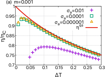
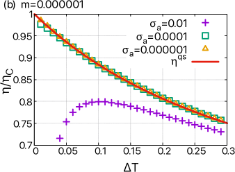
Figure 2: The ratio of the efficiency in Eq. (81) to the Carnot efficiency in our cycle with the protocol in Eq. (89) when $\tau_{x}$ varies at (a) $\tau_{v}=10^{-3}$ and (b) $\tau_{v}=10^{-6}$. Because the parameter $\sigma_{a}$ is proportional to $\tau_{x}(0)$ in the protocol in Eq. (89), we vary $\sigma_{a}$ to make $\tau_{x}$ small. Similarly, we vary the mass $m$ because it is proportional to $\tau_{v}$. In these simulations, we set $\sigma_{a}=10^{-2}$ (purple plus), $\sigma_{a}=10^{-4}$ (green square), and $\sigma_{a}=10^{-6}$ (orange triangle). The red solid line corresponds to the ratio of $\eta^{qs}$ in Eq. (64) to the Carnot efficiency. The efficiency appears to approach the Carnot efficiency in the vanishing limit of $\sigma_{a}$ (or $\tau_{x}$), $m$ (or $\tau_{v}$), and $\Delta T$.

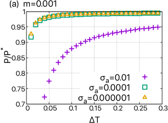
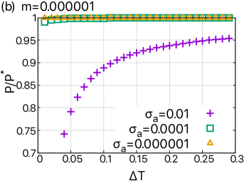
Figure 3: The ratio of the power in Eq. (82) to $P^{*}$ in Eq. (92) in the proposed cycle corresponding to Figs. 2(a) and 2(b). The power appears to approach $P^{*}$ in Eq. (92) in the vanishing limit of $\sigma_{a}$ (or $\tau_{x}$), $m$ (or $\tau_{v}$), and $\Delta T$.

Similarly, we evaluate the power in Eq. (82) by using a criterion $P^{*}$ defined as follows:

$$P^{*}\equiv\frac{W^{qs}}{t_{cyc}}=\frac{\Delta T\Delta S^{qs}}{t_{cyc}},$$ (92)

where $W^{qs}$ is the quasistatic work in Eq. (51). Here, we regard the power as finite when the power in Eq. (82) is the same order as $P^{*}$.

Figure 2 shows the ratio of the efficiency of the proposed cycle with the protocol in Eq. (89) to the Carnot efficiency. We can see that the efficiency approaches $\eta^{qs}$ with $\tau_{x},\ \tau_{v}\to 0$. Considering Eqs. (64) and (88), we can expect that the irreversible works disappear. Thus, the efficiency can be regarded as the Carnot efficiency in the small relaxation-times and small temperature-difference regime.

Figure 3 shows the ratio of the power to $P^{*}$ in Eq. (92), corresponding to Fig. 2. At any $\Delta T$, we can see that the power approaches $P^{*}$ as $\tau_{x},\ \tau_{v}\to 0$ . As the power in Eq. (82) is defined using the work in Eq. (80), the ratio of $P$ to $P^{*}$ is the same as the ratio of $W$ to $W^{qs}$ in Eq. (51). When the power $P$ approaches $P^{*}$, the work $W$ approaches $W^{qs}$. This implies that the irreversible works vanish. Because the power is of the same order as $P^{*}$ from Fig. 3, we can consider the power to be finite. Therefore, Figs. 2 and 3 imply that the Carnot efficiency and finite power are compatible in the vanishing limit of the relaxation times in the small temperature-difference regime.

V Theoretical analysis

This section analytically shows that it is possible to achieve the Carnot efficiency in our cycle in the vanishing limit of the relaxation times in the small temperature-difference regime without breaking the trade-off relation in Eq. (2), as implied in the numerical results in Sec. IV.

In general, the efficiency decreases when the entropy production increases, as shown in Eq. (V). As the adiabatic processes have no entropy production because no heat exchange is present, we have only to consider the entropy production in the isothermal processes. In the small relaxation-times regime, the efficiency in Eq. (81) is approximated by that in Eq. (88). If $W^{irr}_{h,c}\to 0$ is satisfied in the vanishing limit of the relaxation times, the efficiency in Eq. (88) approaches the quasistatic efficiency in Eq. (64). As seen in Eq. (65), it is expected that the contribution of the heat leakage to the efficiency can be neglected in the small temperature-difference regime. Thus, the efficiency in Eq. (81) approaches the Carnot efficiency in the small relaxation-times and small temperature-difference regime, and the power in Eq. (82) also approaches $P^{*}$ in Eq. (92) simultaneously.

The numerical results imply that the irreversible works vanish in the vanishing limit of the relaxation times $\tau_{x}$ and $\tau_{v}$. To derive a similar conclusion analytically, we first show that the irreversible works relate to the entropy production given by

$$\Sigma\equiv-\frac{Q_{h}}{T_{h}}-\frac{Q_{c}}{T_{c}}.$$ (93)

Similarly to $\Sigma^{qs}$ in Eq. (52), the entropy production $\Sigma$ is expressed only by an entropy change in the heat baths. In the small relaxation-times regime, we can express $\Sigma$ in Eq. (93) as follows:

$$\Sigma\simeq \frac{-\frac{\Delta T}{2}-T_{h}\Delta S^{qs}+W^{irr}_{h}}{T_{h}}+\frac{\frac{\Delta T}{2}+T_{c}\Delta S^{qs}+W^{irr}_{c}}{T_{c}}$$

$$= \frac{W^{irr}_{h}}{T_{h}}+\frac{W^{irr}_{c}}{T_{c}}+\frac{(\Delta T)^{2}}{2T_{h}T_{c}},$$ (94)

using Eqs. (86) and (87). The last term on the right-hand side of Eq. (V) comes from the heat leakage due to the instantaneous adiabatic processes. From Eq. (V), the entropy production can be regarded as zero in the small temperature-difference regime when the irreversible works vanish. In general, the entropy production in Eq. (93) can also be rewritten as

$$\begin{split}\Sigma=&\frac{Q_{h}}{T_{c}}(\eta_{C}-\eta),\end{split}$$ (95)

where we used Eqs. (1) and (81). This equation shows that the efficiency approaches the Carnot efficiency when the entropy production vanishes. Thus, by using Eqs. (V) and (95), we obtain the efficiency as

$$\eta =\eta_{C}-\frac{T_{c}\Sigma}{Q_{h}}$$

$$\simeq\eta_{C}-\frac{T_{c}}{Q_{h}}\left(\frac{W^{irr}_{h}}{T_{h}}+\frac{W^{irr}_{c}}{T_{c}}\right)+O[(\Delta T)^{2}],$$ (96)

in the small relaxation-times regime. Here, the contribution of the heat leakage to the efficiency is $O[(\Delta T)^{2}]$, and it is negligible in the small temperature-difference regime.

We consider the trade-off relation in Eq. (2) to discuss the compatibility of the Carnot efficiency and finite power in our Brownian Carnot cycle. Using Eq. (95), we can rewrite Eq. (2) as

$$P\leq\frac{\eta T_{c}}{Q_{h}}A\Sigma$$ (97)

in terms of the entropy production $\Sigma$. When the quantity $A\Sigma$ is nonzero in the vanishing limit of the entropy production $\Sigma$, implying that $A$ should diverge, the finite power may be allowed. In fact, when the entropy production $\Sigma$ vanishes in the small temperature-difference regime, the irreversible works should vanish because of Eq. (V). Then, the power in Eq. (82) approaches $P^{*}$ in Eq. (92), which implies that the power is regarded as finite. Thus, we find the expression $A\Sigma$ in our cycle below.

V.1 Trade-off relation between power and efficiency

We derive the trade-off relation in our cycle. To obtain the expression of the entropy production, we use Eqs. (67) and (68) from Ref. [23]. Using the general expression of the entropy production in the Langevin system [31, 32], Dechant and Sasa showed a trade-off relation for the underdamped Langevin system in Ref. [23]. Thus, we can apply their results to our system. Applying Eq. (67) from Ref. [23], we can divide the probability currents in Eqs. (9) and (10) into the reversible parts, $j_{x}^{rev}$ and $j_{v}^{rev}$, and the irreversible parts, $j_{x}^{irr}$ and $j_{v}^{irr}$, as

$$\begin{split}j_{x}(x,v,t)=&j_{x}^{rev}(x,v,t)+j_{x}^{irr}(x,v,t),\\ j_{v}(x,v,t)=&j_{v}^{rev}(x,v,t)+j_{v}^{irr}(x,v,t),\end{split}$$ (98)

where

$$\begin{split}j^{rev}_{x}(x,v,t)\equiv&vp(x,v,t),\hskip 28.45274ptj^{irr}_{x}(x,v,t)\equiv 0,\\ j^{rev}_{v}(x,v,t)\equiv&-\frac{\lambda(t)}{m}xp(x,v,t),\\ j^{irr}_{v}(x,v,t)\equiv&\left(-\frac{\gamma}{m}v-\frac{\gamma T(t)}{m^{2}}\frac{\partial}{\partial v}\right)p(x,v,t).\end{split}$$ (99)

For convenience, we introduce a function $\phi(t)$ to describe the time evolution of the temperature as

$$\begin{split}\frac{1}{T(t)}=&\frac{1}{T_{c}}-\left(\frac{1}{T_{c}}-\frac{1}{T_{h}}\right)\phi(t)\\ =&\frac{1}{T_{c}}\left[1-\eta_{C}\phi(t)\right].\end{split}$$ (100)

In our cycle, the function $\phi(t)$ is given by

$$\phi(t)\equiv\left\{\begin{split}&1\hskip 8.53581pt(0<t<t_{h})\\ &0\hskip 8.53581pt(t_{h}<t<t_{cyc}).\end{split}\right.$$ (101)

Using Eq. (8), the heat flux in Eq. (18) is rewritten as

$$\dot{Q}= \int^{\infty}_{-\infty}dx\int^{\infty}_{-\infty}dv\left[\frac{1}{2}mv^{2}+\frac{1}{2}\lambda x^{2}\right]\frac{\partial p}{\partial t}$$

$$= -\int^{\infty}_{-\infty}dx\int^{\infty}_{-\infty}dv\left[\frac{1}{2}mv^{2}+\frac{1}{2}\lambda x^{2}\right]\left(\frac{\partial j_{x}}{\partial x}+\frac{\partial j_{v}}{\partial v}\right)$$

$$= \int^{\infty}_{-\infty}dx\int^{\infty}_{-\infty}dv\left[mvj_{v}+\lambda xj_{x}\right],$$ (102)

where the last equality is derived from the integration by parts and we assumed that the probability currents at the boundary vanish. By using Eqs. (98), (99), and (V.1), we obtain the heat flux as

$$\begin{split}\dot{Q}(t)=&\int^{\infty}_{-\infty}dx\int^{\infty}_{-\infty}dv\ mvj_{v}^{irr}(x,v,t).\end{split}$$ (103)

Thus, we obtain the heat flowing from the heat bath to the Brownian particle in the hot isothermal process as

$$\begin{split}Q_{h}=&\int^{t_{h}}_{0}dt\ \int^{\infty}_{-\infty}dx\int^{\infty}_{-\infty}dv\ mvj_{v}^{irr}\\ =&\int^{t_{cyc}}_{0}dt\ \int^{\infty}_{-\infty}dx\int^{\infty}_{-\infty}dv\ \phi(t)mvj_{v}^{irr},\end{split}$$ (104)

using Eq. (101). Now, we consider the entropy production rate. Based on Eq. (68) from Ref. [23], the entropy production rate is given by [31, 32]

$$\begin{split}\dot{\Sigma}(t)=&\int^{\infty}_{-\infty}dx\int^{\infty}_{-\infty}dv\ \frac{m^{2}(j_{v}^{irr}(x,v,t))^{2}}{\gamma T(t)p(x,v,t)}.\end{split}$$ (105)

Using Eq. (105), we can also obtain the concrete expression of the entropy production per cycle as

$$\begin{split}\Sigma=&\int^{t_{cyc}}_{0}dt\ \dot{\Sigma}(t)\\ =&\int^{t_{cyc}}_{0}dt\ \int^{\infty}_{-\infty}dx\int^{\infty}_{-\infty}dv\ \frac{m^{2}(j_{v}^{irr}(x,v,t))^{2}}{\gamma T(t)p(x,v,t)}.\end{split}$$ (106)

From the Cauchy–Schwarz inequality, it is shown that the upper bound of the heat flux in Eq. (103) is expressed using the entropy production rate as

$$\begin{split}\dot{Q}^{2}=&\left(\int^{\infty}_{-\infty}dx\int^{\infty}_{-\infty}dv\ v\sqrt{\gamma Tp}\frac{mj_{v}^{irr}}{\sqrt{\gamma Tp}}\right)^{2}\\ \leq&\left(\int^{\infty}_{-\infty}dx\int^{\infty}_{-\infty}dv\ \gamma Tv^{2}p\right)\\ &\times\left(\int^{\infty}_{-\infty}dx\int^{\infty}_{-\infty}dv\ \frac{m^{2}(j_{v}^{irr})^{2}}{\gamma Tp}\right)\\ =&\gamma T\sigma_{v}\dot{\Sigma},\end{split}$$ (107)

or, equivalently,

$$|\dot{Q}|\leq\sqrt{\gamma T\sigma_{v}\dot{\Sigma}}.$$ (108)

Because $\gamma T(t)\sigma_{v}$ and $\dot{\Sigma}$ are positive, by using Eq. (108), we can derive the following bound for the heat in Eq. (104):

$$\begin{split}(Q_{h})^{2}=&\left(\int^{t_{cyc}}_{0}dt\ \phi(t)\ \dot{Q}(t)\right)^{2}\\ \leq&\left(\int^{t_{cyc}}_{0}dt\ \phi(t)\sqrt{\gamma T(t)\sigma_{v}\dot{\Sigma}}\right)^{2}\\ \leq&\left(\int^{t_{cyc}}_{0}dt\ \phi^{2}(t)\gamma T(t)\sigma_{v}\right)\left(\int^{t_{cyc}}_{0}dt\ \dot{\Sigma}\right)\\ =&t_{cyc}T_{c}^{2}\chi\Sigma,\end{split}$$ (109)

where

$$\chi\equiv\frac{\gamma}{t_{cyc}T_{c}}\int^{t_{cyc}}_{0}dt\ \frac{\phi^{2}(t)}{1-\eta_{C}\phi(t)}\sigma_{v}(t),$$ (110)

and we used the Cauchy–Schwarz inequality and Eq. (100). Using Eqs. (95) and (109), we can derive the trade-off relation in our cycle as

$$\begin{split}P=&\frac{W}{t_{cyc}}=\frac{W}{Q_{h}}\frac{1}{Q_{h}}\frac{Q_{h}^{2}}{t_{cyc}}\\ \leq&\eta\frac{1}{Q_{h}}T_{c}^{2}\chi\Sigma\\ =&\chi T_{c}\eta(\eta_{C}-\eta).\end{split}$$ (111)

By comparing Eqs. (97) and (111), we obtain $A=T_{c}\chi$. We will show that in the limit of $\tau_{x},\tau_{v}\to 0$, the entropy production $\Sigma$ vanishes and $\chi$ diverges while $\chi\Sigma$ maintains positive. For this purpose, we rewrite Eq. (105) as follows. In our model (Sec. II), the probability distribution was assumed to be the Gaussian distribution shown in Eq. (14). Thus, we can differentiate the distribution function $p(x,v,t)$ with respect to $v$ as

$$\frac{\partial p}{\partial v}=\frac{\sigma_{xv}x-\sigma_{x}v}{\sigma_{x}\sigma_{v}-\sigma_{xv}^{2}}p.$$ (112)

We can rewrite the entropy production rate in Eq. (105) by using the variables $\sigma_{x}$, $\sigma_{v}$, and $\sigma_{xv}$ and derive the expression of $\dot{\Sigma}$ under the assumption of the Gaussian distribution as

$$\dot{\Sigma}(t)= \int^{\infty}_{-\infty}dx\int^{\infty}_{-\infty}dv\ \frac{m^{2}}{\gamma Tp}\left\{\left(\frac{\gamma}{m}v+\frac{\gamma T}{m^{2}}\frac{\partial}{\partial v}\right)p\right\}^{2}$$

$$= \frac{m^{2}}{\gamma T}\int^{\infty}_{-\infty}dx\int^{\infty}_{-\infty}dv\left\{\frac{\gamma}{m}v+\frac{\gamma T}{m^{2}}\frac{\sigma_{xv}x-\sigma_{x}v}{\sigma_{x}\sigma_{v}-\sigma_{xv}^{2}}\right\}^{2}p$$

$$= \frac{\frac{\gamma}{m}\left(T-m\sigma_{v}\right)^{2}+(2T-m\sigma_{v})\gamma\frac{\sigma_{xv}^{2}}{\sigma_{x}}}{T\left(m\sigma_{v}-\tau_{v}\gamma\frac{\sigma_{xv}^{2}}{\sigma_{x}}\right)},$$ (113)

where we used Eqs. (6), (7), (12), (18), (99), and (112). Using Eqs. (12) and (18), we obtain

$$\dot{Q}=\frac{\gamma}{m}(T-m\sigma_{v}).$$ (114)

Thus, Eq. (V.1) can be rewritten as

$$\begin{split}\dot{\Sigma}(t)=&\frac{\tau_{v}\dot{Q}^{2}+(2T-m\sigma_{v})\gamma\frac{\sigma_{xv}^{2}}{\sigma_{x}}}{T\left(m\sigma_{v}-\tau_{v}\gamma\frac{\sigma_{xv}^{2}}{\sigma_{x}}\right)}.\end{split}$$ (115)

Integrating Eq. (115) with respect to time, we derive the entropy production per cycle $\Sigma$ in our cycle as

$$\Sigma=\int^{t_{cyc}}_{0}dt\frac{\tau_{v}\dot{Q}^{2}(t)+[2T(t)-m\sigma_{v}(t)]\gamma\frac{\sigma_{xv}^{2}(t)}{\sigma_{x}(t)}}{T(t)\left(m\sigma_{v}(t)-\tau_{v}\gamma\frac{\sigma_{xv}^{2}(t)}{\sigma_{x}(t)}\right)}.$$ (116)

V.2 Small relaxation-times regime

We evaluate the entropy production in Eq. (116) in the small relaxation-times regime. In the hot isothermal process, the process can be divided into the relaxation part and the part after the relaxation. Because the relaxation time of the system at the beginning of the hot isothermal process is given by $\tau_{0}\equiv\max(\tau_{x}(0),\tau_{v})$, the entropy production in the hot isothermal process $\Sigma_{h}$ is divided as

$$\Sigma_{h}\equiv\int^{t_{h}}_{0}dt\ \dot{\Sigma}=\int^{\tau_{0}}_{0}dt\ \dot{\Sigma}+\int^{t_{h}}_{\tau_{0}}dt\ \dot{\Sigma},$$ (117)

where the first and second terms in Eq. (117) represent the entropy production in the relaxation and after the relaxation, respectively. We first evaluate the entropy production after the relaxation. From Eqs. (A151) and (A156) in the Appendix, the variables $\sigma_{x}$, $\sigma_{v}$, and $\sigma_{xv}$ after the relaxation satisfy

$$\sigma_{x}\simeq\frac{T}{\lambda},\quad\sigma_{v}\simeq\frac{T}{m},\quad\sigma_{xv}\simeq-\frac{T}{2\lambda^{2}}\frac{d\lambda}{dt}.$$ (118)

Then, we can obtain

$$\gamma\frac{\sigma_{xv}^{2}(t)}{\sigma_{x}(t)}\simeq\frac{\tau_{x}(t)T}{4}\left(\frac{d}{dt}\ln\lambda(t)\right)^{2}.$$ (119)

Using Eqs. (115), (118), and (119), the entropy production rate after the relaxation is given by

$$\begin{split}\dot{\Sigma}(t)\simeq&\frac{1}{t_{cyc}T}\frac{\frac{\tau_{v}}{t_{cyc}}\left(\frac{dQ(s)}{ds}\right)^{2}+\frac{\tau_{x}}{t_{cyc}}\frac{T^{2}}{4}\left(\frac{d}{ds}\ln\Lambda\right)^{2}}{T-\frac{\tau_{v}}{t_{cyc}}\frac{\tau_{x}}{t_{cyc}}\frac{T}{4}\left(\frac{d}{ds}\ln\Lambda\right)^{2}},\end{split}$$ (120)

where we used $s=t/t_{cyc}$ to compare the cycle time $t_{cyc}$ and the relaxation times $\tau_{x}$ and $\tau_{v}$. Then, we derive the entropy production after the relaxation in the hot isothermal process as

$$\int^{t_{h}}_{\tau_{0}}dt\ \dot{\Sigma}\simeq\frac{1}{T_{h}}\int^{t_{h}/t_{cyc}}_{\tau_{0}/t_{cyc}}ds\ \frac{\frac{\tau_{v}}{t_{cyc}}\left(\frac{dQ(s)}{ds}\right)^{2}+\frac{\tau_{x}}{t_{cyc}}\frac{T_{h}^{2}}{4}\left(\frac{d}{ds}\ln\Lambda\right)^{2}}{T_{h}-\frac{\tau_{v}}{t_{cyc}}\frac{\tau_{x}}{t_{cyc}}\frac{T_{h}}{4}\left(\frac{d}{ds}\ln\Lambda\right)^{2}}.$$ (121)

To consider the entropy production in the relaxation, we rewrite $\dot{\Sigma}$ in Eq. (115) by using the heat flux in Eq. (18) and the time derivative of the entropy in Eq. (II.1) as follows:

$$\dot{\Sigma}(t)=\dot{S}(t)-\frac{\dot{Q}(t)}{T(t)}.$$ (122)

Because the temperature of the heat bath is constant, we derive the entropy production in the relaxation in the hot isothermal process as

$$\int^{\tau_{0}}_{0}dt\ \dot{\Sigma}=S(\tau_{0})-S(0)-\frac{Q^{rel}_{h}}{T_{h}},$$ (123)

where $Q^{rel}_{h}$ is the heat flowing in this relaxation. In the small relaxation-times regime, the relaxation is very fast (see the Appendix), and the stiffness is regarded to be unchanged in the relaxation because of Eq. (A153). From Eq. (A151), $\sigma_{x}$ is also unchanged during the relaxation under the condition of Eq. (57). Thus, the heat related to the potential change in Eq. (20) in the relaxation vanishes. By using Eqs. (19) and (85), $Q^{rel}_{h}$ is evaluated as

$$Q^{rel}_{h}\simeq\frac{\Delta T}{2}.$$ (124)

In addition because $d(\ln\Lambda)/ds$ is noninfinite, as shown in the Appendix, we can approximate the entropy in Eq. (II.1) after the relaxation by

$$S(t)\simeq\frac{1}{2}\ln(T^{2}(t))+\frac{1}{2}\ln\left(\frac{4\pi^{2}}{m\lambda(t)}\right)+1,$$ (125)

where we used the approximation

$$m\lambda(\sigma_{x}\sigma_{v}-\sigma_{xv}^{2})\simeq T^{2}-\frac{\tau_{x}}{t_{cyc}}\frac{\tau_{v}}{t_{cyc}}\frac{T^{2}}{4}\left(\frac{d}{ds}\ln\Lambda\right)^{2}\simeq T^{2},$$ (126)

from Eqs. (24) and (118). The initial state of the hot isothermal process is given by the final state of the cold isothermal process as

$$\sigma_{x}\simeq\frac{T_{c}}{\lambda_{D}},\quad\sigma_{v}\simeq\frac{T_{c}}{m},\quad\sigma_{xv}\simeq-\frac{T_{c}}{2\lambda_{D}^{2}}\left.\frac{d\lambda}{dt}\right|_{t=t_{cyc}-0},$$ (127)

from Eq. (118). Because the stiffness remains $\lambda_{A}$ in the relaxation, the variables relax to the following values:

$$\sigma_{x}\simeq\frac{T_{h}}{\lambda_{A}},\quad\sigma_{v}\simeq\frac{T_{h}}{m},\quad\sigma_{xv}\simeq-\frac{T_{h}}{2\lambda_{A}^{2}}\left.\frac{d\lambda}{dt}\right|_{t=0+0},$$ (128)

from Eq. (118). Using Eqs. (125)–(128), the difference between $S(0)$ and $S(\tau_{0})$ can be approximated by

$$S(\tau_{0})-S(0)\simeq\frac{1}{2}\ln(T_{h}^{2})-\frac{1}{2}\ln(T_{c}^{2})+\frac{1}{2}\ln\left(\frac{\lambda_{D}}{\lambda_{A}}\right).$$ (129)

We can then evaluate the entropy production in the relaxation in Eq. (123) as

$$\int^{\tau_{0}}_{0}dt\ \dot{\Sigma}\simeq \frac{1}{2}\ln(T_{h}^{2})-\frac{1}{2}\ln(T_{c}^{2})+\frac{1}{2}\ln\left(\frac{\lambda_{D}}{\lambda_{A}}\right)-\frac{\Delta T}{2T_{h}}$$

$$= \frac{1}{2}\ln\left(\frac{T_{h}}{T_{c}}\right)-\frac{\Delta T}{2T_{h}},$$ (130)

using Eqs. (57), (66), (124), and (129). Thus, by using Eqs. (121) and (V.2), the entropy production in the hot isothermal process in Eq. (117) is given by

$$\Sigma_{h}\simeq \frac{1}{2}\ln\left(\frac{T_{h}}{T_{c}}\right)-\frac{\Delta T}{2T_{h}}$$ (131)

$$+\frac{1}{T_{h}}\int^{t_{h}/t_{cyc}}_{\tau_{0}/t_{cyc}}ds\ \frac{\frac{\tau_{v}}{t_{cyc}}\left(\frac{dQ(s)}{ds}\right)^{2}+\frac{\tau_{x}}{t_{cyc}}\frac{T_{h}^{2}}{4}\left(\frac{d}{ds}\ln\Lambda\right)^{2}}{T_{h}-\frac{\tau_{v}}{t_{cyc}}\frac{\tau_{x}}{t_{cyc}}\frac{T_{h}}{4}\left(\frac{d}{ds}\ln\Lambda\right)^{2}}.$$

Similarly, the entropy production in the cold isothermal process $\Sigma_{c}$ is given by

$$\Sigma_{c}\equiv \int^{t_{cyc}}_{t_{h}}dt\ \dot{\Sigma}\simeq\frac{1}{2}\ln\left(\frac{T_{c}}{T_{h}}\right)+\frac{\Delta T}{2T_{c}}$$ (132)

$$+ \frac{1}{T_{c}}\int^{1}_{(t_{h}+\tau_{1})/t_{cyc}}ds\ \frac{\frac{\tau_{v}}{t_{cyc}}\left(\frac{dQ(s)}{ds}\right)^{2}+\frac{\tau_{x}}{t_{cyc}}\frac{T_{c}^{2}}{4}\left(\frac{d}{ds}\ln\Lambda\right)^{2}}{T_{c}-\frac{\tau_{v}}{t_{cyc}}\frac{\tau_{x}}{t_{cyc}}\frac{T_{c}}{4}\left(\frac{d}{ds}\ln\Lambda\right)^{2}},$$

where $\tau_{1}\equiv\max(\tau_{x}(t_{h}+0),\tau_{v})$ is the relaxation time at the beginning of the cold isothermal process. Because no entropy production is present in the adiabatic processes, the entropy production $\Sigma$ per cycle in the small relaxation-times regime is given by

$$\Sigma= \Sigma_{h}+\Sigma_{c}$$

$$\simeq \frac{1}{T_{h}}\int^{t_{h}/t_{cyc}}_{\tau_{0}/t_{cyc}}ds\ \frac{\frac{\tau_{v}}{t_{cyc}}\left(\frac{dQ(s)}{ds}\right)^{2}+\frac{\tau_{x}}{t_{cyc}}\frac{T_{h}^{2}}{4}\left(\frac{d}{ds}\ln\Lambda\right)^{2}}{T_{h}-\frac{\tau_{v}}{t_{cyc}}\frac{\tau_{x}}{t_{cyc}}\frac{T_{h}}{4}\left(\frac{d}{ds}\ln\Lambda\right)^{2}}$$

$$+ \frac{1}{T_{c}}\int^{1}_{(t_{h}+\tau_{1})/t_{cyc}}ds\ \frac{\frac{\tau_{v}}{t_{cyc}}\left(\frac{dQ(s)}{ds}\right)^{2}+\frac{\tau_{x}}{t_{cyc}}\frac{T_{c}^{2}}{4}\left(\frac{d}{ds}\ln\Lambda\right)^{2}}{T_{c}-\frac{\tau_{v}}{t_{cyc}}\frac{\tau_{x}}{t_{cyc}}\frac{T_{c}}{4}\left(\frac{d}{ds}\ln\Lambda\right)^{2}}$$

$$+ \frac{(\Delta T)^{2}}{2T_{h}T_{c}},$$ (133)

using Eqs. (131) and (132).

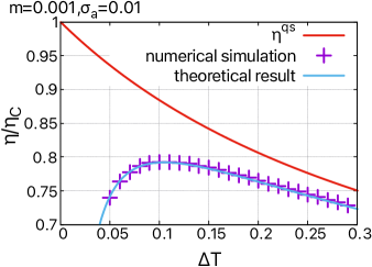
Figure 4: The ratio of the efficiency to the Carnot efficiency derived from the numerical simulations in Fig. 2 in Sec. IV (purple plus) and theoretical analysis (sky-blue solid line). We set $m=10^{-3}$ and $\sigma_{a}=10^{-2}$. Although the relaxation times corresponding to these parameters are not very small among the parameters used in Fig. 2, the theoretical result and numerical simulations show a good agreement. We have confirmed a better agreement with smaller parameters (data not shown).

Comparing Eqs. (V) and (V.2), we can derive the expression of the irreversible works as

$$W^{irr}_{h}= \int^{t_{h}/t_{cyc}}_{\tau_{0}/t_{cyc}}ds\ \frac{\frac{\tau_{v}}{t_{cyc}}\left(\frac{dQ(s)}{ds}\right)^{2}+\frac{\tau_{x}}{t_{cyc}}\frac{T_{h}^{2}}{4}\left(\frac{d}{ds}\ln\Lambda\right)^{2}}{T_{h}-\frac{\tau_{v}}{t_{cyc}}\frac{\tau_{x}}{t_{cyc}}\frac{T_{h}}{4}\left(\frac{d}{ds}\ln\Lambda\right)^{2}},$$ (134)

$$W^{irr}_{c}= \int^{1}_{(t_{h}+\tau_{1})/t_{cyc}}ds\ \frac{\frac{\tau_{v}}{t_{cyc}}\left(\frac{dQ(s)}{ds}\right)^{2}+\frac{\tau_{x}}{t_{cyc}}\frac{T_{c}^{2}}{4}\left(\frac{d}{ds}\ln\Lambda\right)^{2}}{T_{c}-\frac{\tau_{v}}{t_{cyc}}\frac{\tau_{x}}{t_{cyc}}\frac{T_{c}}{4}\left(\frac{d}{ds}\ln\Lambda\right)^{2}}.$$ (135)

As shown in the Appendix, $dQ/ds$ and $d(\ln\Lambda)/ds$ are noninfinite after the relaxation. Thus, the entropy production rate in Eq. (120) after the relaxation vanishes in the vanishing limit of the relaxation times. From Eqs. (134) and (135), it turns out that the integrand of $W^{irr}_{h,c}$, which is $T_{h,c}\dot{\Sigma}$, vanishes at any $s$ in the vanishing limit of the relaxation times, and the irreversible works also vanish. Therefore, we can confirm that the efficiency in Eq. (88) approaches the quasistatic efficiency in Eq. (64) in this limit, theoretically explaining the results of the numerical simulations. Figure 4 compares the efficiency obtained from the numerical simulations in Fig. 2 and the efficiency derived from the theoretical analysis in the small relaxation-times regime. Here, the efficiency of the theoretical analysis was derived by calculating the irreversible works in Eqs. (134) and (135) and substituting them into Eq. (88). Note that we used Eq. (A157) to calculate $dQ/ds$ in Eqs. (134) and (135). We can see that the theoretical result and numerical simulations show a good agreement.

We provide a qualitative explanation for the behavior of the efficiency in Figs. 2 and 4, as below. We consider the case that the relaxation times are small but finite. Then, from the above discussion, $W^{irr}_{h}$ and $W^{irr}_{c}$ are positive and small. When $\Delta T$ is large, $\Delta T\Delta S^{qs}$ in the numerator of Eq. (88) is sufficiently larger than $W^{irr}_{h,c}$ since we use the protocol satisfying $\Delta S^{qs}=O(1)$ in the numerical simulation. Since $T_{h}$ is larger than $\Delta T$, $T_{h}\Delta S^{qs}$ in the denominator of Eq. (88) is also sufficiently larger than $W^{irr}_{h,c}$. Thus, the efficiency should mainly depend on $T_{h}$, $\Delta T$, and $\Delta S^{qs}$ as shown in Eq. (88). Although the efficiency is smaller than the Carnot efficiency because of $\Delta T/2$ due to the heat leakage in the denominator of Eq. (88), the heat leakage becomes small and the efficiency increases toward the Carnot efficiency as $\Delta T$ becomes small. At the same time, however, the irreversible works can be comparable to $\Delta T\Delta S^{qs}$. From Eq. (89), the stiffness in each isothermal process depends only on the corresponding temperature. Since $dQ/ds$ in Eqs. (134) and (135) is evaluated by the protocol as shown in Eq. (A157), $W^{irr}_{h,c}$ depend only on the temperature of each isothermal process, but do not depend on $\Delta T$ in the lowest order of $\Delta T$. Thus, the irreversible works maintain finite even when $\Delta T$ vanishes. Then, $\Delta T\Delta S^{qs}$ in Eq.(88) approaches zero while $W^{irr}_{h,c}$ are positively finite. Thus, the efficiency turns from increase to decrease as $\Delta T$ becomes small and takes the maximum for a specific value of $\Delta T$ as shown in Figs. 2 and 4.

By using $s=t/t_{cyc}$, the quantity $\phi(t)$ in Eq. (101) can be expressed as

$$\phi(s)=\left\{\begin{split}&1\hskip 8.53581pt(0<s<t_{h}/t_{cyc})\\ &0\hskip 8.53581pt(t_{h}/t_{cyc}<s<1).\end{split}\right.$$ (136)

Thus, $\chi$ in Eq. (110) is rewritten by using the relaxation time of the velocity as

$$\chi=\frac{1}{t_{cyc}}\frac{t_{cyc}}{\tau_{v}}\left(\frac{1}{T_{c}}\int^{1}_{0}ds\ \frac{m\sigma_{v}\phi^{2}}{1-\eta_{C}\phi}\right)=\frac{C}{t_{cyc}}\frac{t_{cyc}}{\tau_{v}},$$ (137)

where $C$ is a positive constant given by

$$C\equiv\frac{1}{T_{c}}\int^{1}_{0}ds\ \frac{m\sigma_{v}\phi^{2}}{1-\eta_{C}\phi}.$$ (138)

In the relaxation at the beginning of each isothermal process, $m\sigma_{v}$ is positively finite. After the relaxation, $m\sigma_{v}$ is approximated by the temperature of the heat bath. Thus, $C$ is positively finite. From Eq. (137), $\chi$ turns out to diverge in the limit of $\tau_{v}/t_{cyc}\to 0$ when $t_{cyc}$ is finite. Although $\tau_{v}/t_{cyc}\to 0$ is satisfied even when $t_{cyc}$ diverges and $\tau_{v}$ is maintained finite, we do not consider that case because it is in the quasistatic limit. Using Eqs. (V.2) and (137), we can obtain $\chi\Sigma$ as follows:

$$\chi\Sigma\simeq \frac{C}{t_{cyc}T_{h}}\int^{t_{h}/t_{cyc}}_{\tau_{0}/t_{cyc}}ds\ \frac{\left(\frac{dQ}{ds}\right)^{2}+\frac{\tau_{x}T_{h}^{2}}{4\tau_{v}}\left(\frac{d}{ds}\ln\Lambda\right)^{2}}{T_{h}-\frac{\tau_{v}}{t_{cyc}}\frac{\tau_{x}}{t_{cyc}}\frac{T_{h}}{4}\left(\frac{d}{ds}\ln\Lambda\right)^{2}}$$

$$+\frac{C}{t_{cyc}T_{c}}\int^{1}_{(t_{h}+\tau_{1})/t_{cyc}}ds\ \frac{\left(\frac{dQ}{ds}\right)^{2}+\frac{\tau_{x}T_{c}^{2}}{4\tau_{v}}\left(\frac{d}{ds}\ln\Lambda\right)^{2}}{T_{c}-\frac{\tau_{v}}{t_{cyc}}\frac{\tau_{x}}{t_{cyc}}\frac{T_{c}}{4}\left(\frac{d}{ds}\ln\Lambda\right)^{2}}$$

$$+\frac{C}{\tau_{v}}\frac{(\Delta T)^{2}}{2T_{h}T_{c}}.$$ (139)

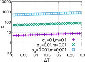
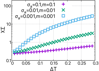
Figure 5: The quantities $\chi$ in Eq. (110) and $\chi\Sigma$ when $\tau_{x}$ and $\tau_{v}$ are varied. Because the parameter $\sigma_{a}$ is proportional to $\tau_{x}(0)$ in the protocol in Eq. (89), we vary $\sigma_{a}$ to make $\tau_{x}$ be small. Similarly, we vary the mass $m$ because it is proportional to $\tau_{v}$. In these simulations, we used $(\sigma_{a}=0.1,m=0.1)$ (purple plus), $(\sigma_{a}=0.01,m=0.01)$ (green cross), and $(\sigma_{a}=0.001,m=0.001)$ (sky-blue square). We can see that $\chi$ diverges at each $\Delta T$ when we consider the limit of $\sigma_{a},m\to 0$ ($\tau_{x},\tau_{v}\to 0$). In addition, we can also see that the values of $\chi\Sigma$ are positively finite for the vanishing limit of $\Delta T$ for any relaxation times.

Here, we consider the vanishing limit of the relaxation times in the small temperature-difference regime and evaluate the efficiency and power in this limit. As seen in Eq. (V), the efficiency approaches the Carnot efficiency when $\Sigma$ vanishes. Moreover, we evaluate $\Sigma$ in the vanishing limit of $\tau_{x}$ and $\tau_{v}$ in the small temperature-difference regime. In this limit, we can show that $dQ/ds$ and $d(\ln\Lambda)/ds$ in Eq. (V.2) do not diverge after the relaxation (see the Appendix). Thus, when the relaxation times vanish at any instant after the relaxation, the entropy production rate always vanishes from Eq. (120), and the first and second terms on the right-hand side of Eq. (V.2) also vanish. In addition, when $\Delta T$ is small, the third term in Eq. (V.2), which is due to the relaxation, is $O[(\Delta T)^{2}]$ and can be ignored. Therefore, the entropy production per cycle in Eq. (V.2) should be $O[(\Delta T)^{2}]$, and the efficiency can be regarded as the Carnot efficiency because of the reasoning presented below Eq. (V). Then, because $dQ/ds$ and $d(\ln\Lambda)/ds$ are always noninfinite, the first and second terms on the right-hand side of Eq. (V.2) are positively finite in the vanishing limit of $\tau_{x}$ and $\tau_{v}$. Even when $\Delta T$ is small, $\chi\Sigma$ is positive, and the right-hand side of the trade-off relation in Eq. (111) is positive. Therefore, the finite power may be allowed even when $\Sigma$ vanishes. In the above limit, because the irreversible works in Eqs. (134) and (135) vanish, the power in Eq. (82) approaches $P^{*}$ in Eq. (92), which implies that the power is finite. Therefore, the Carnot efficiency is achievable in the finite-power Brownian Carnot cycle without breaking the trade-off relation in Eq. (111).

In Fig. 5, we numerically confirmed that $\chi$ increases and $\chi\Sigma$ remains positively finite in the limit of $\Delta T\to 0$ when we consider smaller relaxation times. We can expect $\chi$ to diverge while maintaining $\chi\Sigma$ positively finite in the vanishing limit of the relaxation times in the limit of $\Delta T\to 0$. This result implies that $\Sigma$ vanishes while maintaining $\chi\Sigma$ positively finite, and we can expect that $\Sigma$ vanishes and $\chi$ diverges simultaneously in the vanishing limit of the relaxation times.

VI Summary and discussion

Motivated by the previous study [24], we studied the relaxation-times dependence of the efficiency and power in a Brownian Carnot cycle with the instantaneous adiabatic processes and time-dependent harmonic potential, described by the underdamped Langevin equation. In this system, we numerically showed that the Carnot efficiency is compatible with finite power in the vanishing limit of the relaxation times in the small temperature-difference regime. We analytically showed that the present results are consistent with the trade-off relation between efficiency and power, which was proved for more general systems in [17, 18, 23]. By expressing the trade-off relation using the entropy production in terms of the relaxation times of the system, we demonstrated that such compatibility is possible by both the diverging constant and the vanishing entropy production in the trade-off relation in the vanishing limit of the relaxation times.

In the numerical simulation results in Sec. IV, we used a specific protocol. However, we can use other protocols satisfying the following three conditions to achieve the Carnot efficiency and finite power in the small temperature-difference regime. The first condition is that the protocol should satisfy the condition in Eq. (57). For such a protocol, the heat leakage in the relaxation at the beginning of the isothermal processes is $O(\Delta T)$. Thus, heat leakage can be neglected in the small temperature-difference regime, compared with the heat flowing in the isothermal processes. The second condition is that the stiffness is expressed by using a scaling function as in Eq. (24). The third condition of the protocols is that the stiffness diverges at any instant of time. This is satisfied by the vanishing relaxation time of position, and it is one of the necessary conditions for the entropy production rate vanishing after the relaxation, as we showed in Sec. V. When the entropy production rate at any instant vanishes, irreversible works also vanish, which allows us to derive the compatibility of the Carnot efficiency and finite power in the small temperature-difference regime.

Note that we showed that achieving both the Carnot efficiency and finite power is possible in the small temperature-difference regime without breaking the trade-off relation in Eq. (97) of the proposed cycle. In the linear irreversible thermodynamics, which can describe the heat engines operating in the small temperature-difference regime, the currents of the systems are described by the linear combination of affinities, and their coefficients are called the Onsager coefficients. When these coefficients have the reciprocity resulting from the time-reversal symmetry of the systems, a previous study [7] showed that the compatibility of the Carnot efficiency with finite power is forbidden. The same study also showed that the compatibility can be allowed in the systems without time-reversal symmetry. However, in some studies related to the concrete systems without time-reversal symmetry [8, 9, 10, 11, 12, 13], the compatibility has not been found thus far. On the other hand, there is a possibility of the compatibility of the Carnot efficiency and finite power when the Onsager coefficients with reciprocity show diverging behaviors (cf. Eq. (7) in Ref. [19]). The Onsager coefficients of our Carnot cycle can be obtained in the same way as Ref. [33], which have reciprocity. In the vanishing limit of the relaxation times, we can show the divergence of these Onsager coefficients. Although the effect of the asymmetric limit of the non-diagonal Onsager coefficients on the linear irreversible heat engines realizing the Carnot efficiency at finite power was studied in Ref. [7], this case is different from our case where all of the Onsager coefficients show the diverging behaviors.

Furthermore, another study reported the compatibility of the Carnot efficiency with finite power using a time-delayed system within the linear response theory [34]. Because the time-delayed systems are not described by the Markovian dynamics, the trade-off relation in Eq. (2) may not be applied to them. Thus, there may be a possibility to achieve the Carnot efficiency in finite-power non-Markovian heat engines. In this paper, however, we showed that achieving both the Carnot efficiency and finite power is possible in a Markovian heat engine.

Although we have used the instantaneous adiabatic process, the other type of adiabatic process can be used for the study of the Brownian Carnot cycle [28, 35, 36, 24]. In this adiabatic process, the system contacts with a heat bath with varying temperature that maintains vanishing heat flow between the system and the heat bath on average. While the Brownian Carnot cycle utilizing this adiabatic process does not suffer from the heat leakage, mathematical treatment may become more difficult. Therefore, it is a challenging task to study the detailed relaxation-times dependence of the efficiency and power for this cycle, which we will report elsewhere.

Appendix Behavior of heat flux in the vanishing limit of relaxation times

We show that heat flux $\dot{Q}$ after the relaxation in an isothermal process is noninfinite in the vanishing limit of the relaxation times. For this purpose, we first consider the case where the stiffness $\lambda$ and the temperature $T$ are constant. We assume that an isothermal process lasts for $t_{i}<t<t_{f}$. As the adiabatic processes take no time, the variables $\sigma_{x}$, $\sigma_{v}$, and $\sigma_{xv}$ at the beginning of the isothermal process should be unchanged from the end of the preceding isothermal process. We set $\sigma_{x}(t_{i})=\sigma_{x0}$, $\sigma_{v}(t_{i})=\sigma_{v0}$, and $\sigma_{xv}(t_{i})=\sigma_{xv0}$. Under these initial conditions, we can solve Eqs. (11)–(13) using the Laplace transform [27], and we can obtain $\sigma_{x}$ and $\sigma_{v}$ as follows:

$$\begin{split}\sigma_{x}(t)=&\frac{T}{\lambda}+\frac{m}{\lambda}D_{1}e^{-\frac{\gamma}{m}(t-t_{i})}\\ &+\frac{\left(\gamma+m\omega^{*}\right)^{2}}{4\lambda^{2}}D_{2}e^{-\left(\frac{\gamma}{m}-\omega^{*}\right)(t-t_{i})}\\ &+\frac{\left(\gamma-m\omega^{*}\right)^{2}}{4\lambda^{2}}D_{3}e^{-\left(\frac{\gamma}{m}+\omega^{*}\right)(t-t_{i})},\end{split}$$ (A140)

$$\begin{split}\sigma_{v}(t)=&\frac{T}{m}+D_{1}e^{-\frac{\gamma}{m}(t-t_{i})}+D_{2}e^{-\left(\frac{\gamma}{m}-\omega^{*}\right)(t-t_{i})}\\ &+D_{3}e^{-\left(\frac{\gamma}{m}+\omega^{*}\right)(t-t_{i})},\end{split}$$ (A141)

where

$$\omega^{*}\equiv \frac{\gamma}{m}\sqrt{1-4\frac{m\lambda}{\gamma^{2}}},$$ (A142)

$$D_{1}\equiv \frac{\lambda}{m{\omega^{*}}^{2}}\left(4\frac{T}{m}-2\sigma_{v0}-2\frac{\lambda}{m}\sigma_{x0}-2\frac{\gamma}{m}\sigma_{xv0}\right),$$ (A143)

$$D_{2}\equiv -\frac{1}{2{\omega^{*}}^{2}}\left[\frac{\gamma T}{m^{2}}\left(\frac{\gamma}{m}-\omega^{*}\right)+\left(2\frac{\lambda}{m}-\frac{\gamma^{2}}{m^{2}}+\frac{\gamma}{m}\omega^{*}\right)\sigma_{v0}\right.$$

$$-2\frac{\lambda^{2}}{m^{2}}\sigma_{x0}\left.+2\frac{\lambda}{m}\left(-\frac{\gamma}{m}+\omega^{*}\right)\sigma_{xv0}\right],$$ (A144)

$$D_{3}\equiv -\frac{1}{2{\omega^{*}}^{2}}\left[\frac{\gamma T}{m^{2}}\left(\frac{\gamma}{m}+\omega^{*}\right)+\left(2\frac{\lambda}{m}-\frac{\gamma^{2}}{m^{2}}-\frac{\gamma}{m}\omega^{*}\right)\sigma_{v0}\right.$$

$$-2\frac{\lambda^{2}}{m^{2}}\sigma_{x0}\left.+2\frac{\lambda}{m}\left(-\frac{\gamma}{m}-\omega^{*}\right)\sigma_{xv0}\right].$$ (A145)

We can also derive $\sigma_{xv}$ using Eqs. (13) and (A140). We can rewrite Eq. (A142) using the relaxation times Eqs. (6) and (7) as

$$\omega^{*}=\frac{1}{\tau_{v}}\sqrt{1-4\frac{\tau_{v}}{\tau_{x}}}.$$ (A146)

The exponential functions in Eqs. (A140) and (A141) are represented using $s=t/t_{cyc}$ and the relaxation times as

$$e^{-\frac{\gamma}{m}(t-t_{i})} =e^{-\frac{t_{cyc}}{\tau_{v}}\left(s-\frac{t_{i}}{t_{cyc}}\right)},$$ (A147)

$$e^{-\left(\frac{\gamma}{m}-\omega^{*}\right)(t-t_{i})} =e^{-\frac{t_{cyc}}{\tau_{v}}\left(1-\sqrt{1-4\frac{\tau_{v}}{\tau_{x}}}\right)\left(s-\frac{t_{i}}{t_{cyc}}\right)},$$ (A148)

$$e^{-\left(\frac{\gamma}{m}+\omega^{*}\right)(t-t_{i})} =e^{-\frac{t_{cyc}}{\tau_{v}}\left(1+\sqrt{1-4\frac{\tau_{v}}{\tau_{x}}}\right)\left(s-\frac{t_{i}}{t_{cyc}}\right)}.$$ (A149)

When we consider $\tau_{x}\leq 4\tau_{v}$, $\omega^{*}$ in Eq. (A146) becomes purely imaginary. Thus, the exponential terms in Eqs. (A147)–(A149) vanish in $\tau_{v}/t_{cyc}\to 0$ when $s>t_{i}/t_{cyc}$ is satisfied. When we also consider $\tau_{x}>4\tau_{v}$, the exponential terms in Eqs. (A147) and (A149), vanish in $\tau_{v}/t_{cyc}\to 0$. Because the exponent of Eq. (A148) can be approximated by

$$-\frac{t_{cyc}}{\tau_{v}}\left(1-\sqrt{1-4\frac{\tau_{v}}{\tau_{x}}}\right)\left(s-\frac{t_{i}}{t_{cyc}}\right)\simeq-2\frac{t_{cyc}}{\tau_{x}}\left(s-\frac{t_{i}}{t_{cyc}}\right),$$ (A150)

the exponential terms in Eq. (A148) vanishes in $\tau_{x}/t_{cyc}\to 0$ when $s>t_{i}/t_{cyc}$ is satisfied. Thus, the exponential terms vanish in any value of $\tau_{v}/\tau_{x}$ in the vanishing limit of $\tau_{x}$ and $\tau_{v}$ when $s-t_{i}/t_{cyc}$ is positively finite. Therefore, $\sigma_{x}$ and $\sigma_{v}$ after the relaxation are approximated by

$$\sigma_{x}\simeq\frac{T}{\lambda},\quad\sigma_{v}\simeq\frac{T}{m}.$$ (A151)

To obtain $\sigma_{xv}$, we use Eqs. (11) and (A140) as follows: Because $T$ and $\lambda$ are constant, the time derivative of the first term in Eq. (A140) disappears. Moreover, as the exponential terms vanish rapidly, the remaining terms in Eq. (A140) vanish after the relaxation even when we differentiate them with respect to time. Thus $\sigma_{xv}$ vanishes after the relaxation.

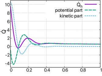
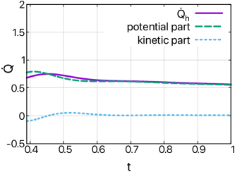
Figure 6: Time evolution of $\dot{Q}_{h}(t)$ (purple solid line), its potential part $\lambda\dot{\sigma}_{x}/2$ (green dashed line), and its kinetic part $m\dot{\sigma}_{v}/2$ (sky-blue dotted line) in the hot isothermal process. We can see a relaxation at the beginning of the process. The lower figure is an enlargement view of a part of the upper figure, which shows that $\dot{Q}_{h}(t)\simeq\lambda(t)\dot{\sigma}_{x}(t)/2$ and $m\dot{\sigma}_{v}(t)\simeq 0$ are satisfied. In this simulation, we used $\lambda(t)$ in Eq. (89) and set $T_{h}=2.0$, $T_{c}=1.0$, $t_{h}=t_{c}=1.0$, $m=0.1$, $\sigma_{a}=0.1$, $\gamma=1.0$, and $\sigma_{b}/\sigma_{a}=2.0$.

Subsequently, we consider the isothermal process where the stiffness $\lambda$ depends on time. When $\tau_{j}$ ($j=x,v$) is sufficiently small, by using the Taylor expansion, we derive

$$\begin{split}\lambda(t+\tau_{j})\simeq\lambda(t)\left(1+\tau_{j}\frac{d}{dt}\ln\lambda(t)\right).\end{split}$$ (A152)

If $d(\ln\lambda)/dt$ is noninfinite in the vanishing limit of $\tau_{j}$, we can obtain

$$\lambda(t+\tau_{j})\simeq\lambda(t),$$ (A153)

which implies that the stiffness $\lambda$ is constant during the relaxation. We show that $d(\ln\lambda)/dt$ is noninfinite as below. Because $\lambda$ varies smoothly in the isothermal process, $\lambda$ is differentiable, and we obtain

$$\frac{\lambda(t+\Delta t)}{\lambda(t)}\simeq 1+\Delta t\frac{d}{dt}\ln\lambda(t),$$ (A154)

where $\Delta t$ is finite but sufficiently small. Because we assumed that $\lambda(t_{f})/\lambda(t_{i})$ is finite at any time $t_{i}$ and $t_{f}$ in the isothermal process, as mentioned below Eq. (24) in Sec. III, $d(\ln\lambda(t))/dt$ should be noninfinite. Thus, as Eq. (A153) is satisfied, we can regard $\lambda$ as a constant in the relaxation even if $\lambda$ varies with time and diverges. Thus, we can apply $\sigma_{x}$ and $\sigma_{v}$ in Eqs. (A140) and (A141) under constant $\lambda$ to the case of varying $\lambda$ in the relaxation. Then, $\sigma_{x}$ and $\sigma_{v}$ immediately relax in the vanishing limit of $\tau_{x}$ and $\tau_{v}$ and satisfy Eq. (A151) immediately after the relaxation. When the stiffness changes from $\lambda(t)$ to $\lambda(t+\Delta t)$ after the relaxation, $\sigma_{x}$ and $\sigma_{v}$ immediately relax to Eq. (A151) with $\lambda=\lambda(t+\Delta t)$ in the limit of $\tau_{x}(t),\tau_{v}\to 0$. Thus, when $\tau_{x}(t)$ and $\tau_{v}$ vanish at any instant, we can regard that Eq. (A151) is always satisfied in the isothermal process after the relaxation. When we consider $\sigma_{xv}$, the time derivative of $T/\lambda$ in Eq. (A140) does not vanish because $\lambda$ varies smoothly. The remaining terms in Eq. (A140) vanish after the relaxation even when we differentiate them with respect to time because the exponential terms vanish rapidly. Using Eq. (A151), we obtain the time evolution of $\sigma_{x}$ and $\sigma_{v}$ after the relaxation in the isothermal process with the temperature $T$ as

$$\dot{\sigma}_{x}(t)\simeq-\frac{T}{\lambda(t)}\left(\frac{d}{dt}\ln\lambda\right),\quad\dot{\sigma}_{v}\simeq 0.$$ (A155)

Then, from Eq. (11), we obtain

$$\sigma_{xv}(t)\simeq-\frac{T}{2\lambda(t)}\left(\frac{d}{dt}\ln\lambda\right).$$ (A156)

The heat flux $\dot{Q}(t)$ in Eq. (18) is represented as

$$\begin{split}\dot{Q}(t)\simeq&\frac{1}{2}\lambda(t)\dot{\sigma}_{x}(t)\simeq-\frac{T}{2}\left(\frac{d}{dt}\ln\lambda\right),\end{split}$$ (A157)

where we used Eq. (A155), and $\dot{Q}$ is noninfinite because $d(\ln\lambda)/dt$ is noninfinite. Note that we obtain

$$\frac{d}{ds}\ln\Lambda= t_{cyc}\frac{d}{dt}\ln\lambda,$$

$$\frac{dQ}{ds}= t_{cyc}\frac{dQ}{dt}=-\frac{T}{2}\left(\frac{d}{ds}\ln\Lambda\right),$$ (A158)

using $s$ and Eqs. (24) and (A157). Because $d(\ln\lambda)/dt$ is noninfinite, $d(\ln\Lambda)/ds$ and $dQ/ds$ are also noninfinite after the relaxation when $t_{cyc}$ is finite.

Figure 6 shows a time evolution of the heat flux $\dot{Q}_{h}$, its potential part $\lambda\dot{\sigma}_{x}/2$, and its kinetic part $m\dot{\sigma}_{v}/2$ in the hot isothermal process with the protocol in Eq. (89). In this simulation, we used the same parameters as in Sec. IV. From the figure, we can see a relaxation at the beginning of the process. As implied in Eq. (A157), the heat flux $\dot{Q}_{h}$ is almost equal to its potential part $\lambda\dot{\sigma}_{x}/2$, and the kinetic part $m\dot{\sigma}_{v}/2$ almost vanishes after the relaxation.

References

- Callen [1985] H. B. Callen, Thermodynamics and an Introduction to Thermostatistics, 2nd ed. (Wiley, New York, 1985).
- Carnot [1824] S. Carnot, Reflections on the Motive Power of Fire and on Machines Fitted to Develop that Power (Bachelier, Paris, 1824).
- Polettini and Esposito [2017] M. Polettini and M. Esposito, Europhys. Lett. 118, 40003 (2017).
- Hondou and Sekimoto [2000] T. Hondou and K. Sekimoto, Phys. Rev. E 62, 6021 (2000).
- Shiraishi [2017] N. Shiraishi, Phys. Rev. E 95, 052128 (2017).
- Campisi and Fazio [2016] M. Campisi and R. Fazio, Nat. Comm. 7, 11895 (2016).
- Benenti et al. [2011] G. Benenti, K. Saito, and G. Casati, Phys. Rev. Lett. 106, 230602 (2011).
- Brandner et al. [2013] K. Brandner, K. Saito, and U. Seifert, Phys. Rev. Lett. 110, 070603 (2013).
- Balachandran et al. [2013] V. Balachandran, G. Benenti, and G. Casati, Phys. Rev. B 87, 165419 (2013).
- Yamamoto et al. [2016] K. Yamamoto, O. Entin-Wohlman, A. Aharony, and N. Hatano, Phys. Rev. B 94, 121402(R) (2016).
- Stark et al. [2014] J. Stark, K. Brandner, K. Saito, and U. Seifert, Phys. Rev. Lett. 112, 140601 (2014).
- Sánchez et al. [2015] R. Sánchez, B. Sothmann, and A. N. Jordan, Phys. Rev. Lett. 114, 146801 (2015).
- Sothmann et al. [2014] B. Sothmann, R. Sánchez, and A. N. Jordan, Europhys. Lett 107, 47003 (2014).
- Ma et al. [2018] Y.-H. Ma, D. Xu, H. Dong, and C.-P. Sun, Phys. Rev. E 98, 042112 (2018).
- Abiuso and Perarnau-Llobet [2020] P. Abiuso and M. Perarnau-Llobet, Phys. Rev. Lett. 124, 110606 (2020).
- Holubec and Ryabov [2017] V. Holubec and A. Ryabov, Phys. Rev. E 96, 062107 (2017).
- Shiraishi et al. [2016] N. Shiraishi, K. Saito, and H. Tasaki, Phys. Rev. Lett. 117, 190601 (2016).
- Shiraishi and Tajima [2017] N. Shiraishi and H. Tajima, Phys. Rev. E 96, 022138 (2017).
- Shiraishi [2018] N. Shiraishi, BusseiKenkyu 7, 072213 (2018), (in Japanese).
- Pietzonka and Seifert [2018] P. Pietzonka and U. Seifert, Phys. Rev. Lett. 120, 190602 (2018).
- Koyuk et al. [2018] T. Koyuk, U. Seifert, and P. Pietzonka, J. Phys. A: Math. Theor. 52, 02LT02 (2018).
- Dechant [2018] A. Dechant, J. Phys. A: Math. Theor. 52, 035001 (2018).
- Dechant and Sasa [2018] A. Dechant and S.-i. Sasa, Phys. Rev. E 97, 062101 (2018).
- Holubec and Ryabov [2018] V. Holubec and A. Ryabov, Phys. Rev. Lett. 121, 120601 (2018).
- Dechant et al. [2017] A. Dechant, N. Kiesel, and E. Lutz, Europhys. Lett. 119, 50003 (2017).
- Schmiedl and Seifert [2007] T. Schmiedl and U. Seifert, Europhys. Lett. 81, 20003 (2007).
- Arold et al. [2018] D. Arold, A. Dechant, and E. Lutz, Phys. Rev. E 97, 022131 (2018).
- Plata et al. [2020a] C. A. Plata, D. Guéry-Odelin, E. Trizac, and A. Prados, Phys. Rev. E 101, 032129 (2020a).
- Risken [1996] H. Risken, The Fokker-Planck Equation, 2nd ed. (Springer, New York, 1996).
- [30] K. Sekimoto, Stochastic Energetics, Lecture Notes in Physics (Springer, Berlin, Heidelberg).
- Seifert [2012] U. Seifert, Rep. Prog. Phys. 75, 126001 (2012).
- Spinney and Ford [2012] R. E. Spinney and I. J. Ford, Phys. Rev. E 85, 051113 (2012).
- Izumida and Okuda [2010] Y. Izumida and K. Okuda, Eur. Phys. J. B 77, 499 (2010).
- Bonança [2019] M. V. S. Bonança, J. Stat. Mech. 2019, 123203 (2019).
- Plata et al. [2020b] C. A. Plata, D. Guéry-Odelin, E. Trizac, and A. Prados, J. Stat. Mech. 2020, 093207 (2020b).
- Martínez et al. [2015] I. A. Martínez, E. Roldán, L. Dinis, D. Petrov, and R. A. Rica, Phys. Rev. Lett. 114, 120601 (2015).