Deep Discriminative Feature Learning for Accent Recognition

Abstract

Accent recognition with deep learning framework is a similar work to deep speaker identification, they’re both expected to give the input speech an identifiable representation. Compared with the individual-level features learned by speaker identification network, the deep accent recognition work throws a more challenging point that forging group-level accent features for speakers. In this paper, we borrow and improve the deep speaker identification framework to recognize accents, in detail, we adopt Convolutional Recurrent Neural Network as front-end encoder and integrate local features using Recurrent Neural Network to make an utterance-level accent representation. Novelly, to address overfitting, we simply add Connectionist Temporal Classification based speech recognition auxiliary task during training, and for ambiguous accent discrimination, we introduce some powerful discriminative loss functions in face recognition works to enhance the discriminative power of accent features. We show that our proposed network with discriminative training method (without data-augment) is significantly ahead of the baseline system on the accent classification track in the Accented English Speech Recognition Challenge 2020, where the loss function Circle-Loss has achieved the best discriminative optimization for accent representation.

Index Terms: accent recognition, deep feature learning, speaker recognition

1 Introduction

Under a particular language, the accent is a learned or behavioral speaking property which can be influenced by social status, education and residence area [1], where the accent we mainly concern is caused by the regional factor. Accent recognition (AR) technologies [2, 3, 4, 5, 6, 7], which can be used to targetedly address accent-related problems or predict a creditable identity for the speaker to make customized service, have attracted extensive attention in recent years. In this paper, we design a deep framework with discriminative feature learning method on the accent classification track of Accented English Speech Recognition Challenge 2020 (AESRC2020) [8], where the English speech accents in data-set derive from 8 countries. Unlike many solutions, which concentrate on preprocessings (e.g. top-1 scheme [9] in AESRC2020), on the basis of the Fbank input-feature and the raw data, we focus on the discriminative model optimization to improve accent classification accuracy.

In deep feature learning, AR task is similar to speaker identification (SI) [10, 11, 12, 13] and language identification (LI) [14, 15, 16], they both want to give the input speech a distinguishable representation. In the modeling method, they could share the same deep paradigm [12, 13]: (i) employing deep neural network (DNN) to extract frame-level feature, (ii) temporal integration of frame-level features, and (iii) discriminative feature learning. In our work, taking the 2D speech spectrogram as input, we use Convolutional Recurrent Neural Network (CRNN) [17] to extract frame-level descriptors, specifically, our CRNN based extractor is composed of ResNet [18] and Bidirectional GRU [19] (BiGRU) network, nextly, the calculated local descriptors are integrated into a global utterance-level feature using BiGRU. However, to learn the group-level accent feature for many speakers is harder than to learn individual-level speaker feature. Concretely, this difficulty is reflected in:

1. Overfitting: Under the limited training-data, due to the number of accents is far less than the number of speakers and the input speech contains rich and varied signals, fast convergence under this petty classification target is not equivalent to obtain accurate accent representation. Hence, the learned decision path may be inaccurate even though it works perfectly on closed-set.

2. Difficult Accent Detection: In many formal social situations, speakers tend to adopt standardized pronunciation (e.g. the mandarin in Chinese), this pronunciation will narrow the differences between different accents and make accent recognition harder. In another view, this indistinguishable accent leads to ambiguous embedding representation in deep network.

In order to solve the above two problems, we improve the deep paradigm with the following two solutions: (i) For issue 1, we adopt multitask learning (MTL) training method, that is, we introduce Automatic Speech Recognition (ASR) auxiliary task where we simply add Connectionist Temporal Classification (CTC) based ASR decoder onto the front-end encoder during training. (ii) For issue 2, we employ some popular discriminative loss functions [20, 21, 22, 23] in face recognition (FR) works to strengthen the discriminative power of accent feature. In addition to the state-of-the-art discriminative optimization works in SI [12, 13, 24, 25], we further introduce the loss: Circle-Loss [23], an improvement for the problem of inflexible optimization and ambiguous convergence status, to achieve better performance in our experiments.

2 Deep Classification Architecture

We borrow and improve the deep SI framework [12, 13] to forge utterance-level representation for accent classification. As Figure 1 shows, taking a 2D spectrogram as input, the proposed deep accent recognition network is composed of: (1) a CRNN based front-end encoder to extract frame-level descriptors, constructed with the ResNet based CNN subpart and the BiGRU based RNN subpart; (2) a feature integration layer to integrate arbitrary frame-level local features into an utterance-level global feature vector; (3) a discriminative loss function during training to enhance the discriminative power of global accent feature; (4) a softmax-based classifier, attached to the global feature and give the posterior distribution of accents; The above 2, 3, and 4 components make up the AR branch. To tackle the overfitting issue, we add an ASR branch behind the front-end encoder during training where we simply adopt CTC objective. Overall, our model has three outputs (the rectangles with red box in Figure 1) during training, among which the prediction is given by the softmax-based classifier. We will give the detailed modeling explanation in the following subsections.

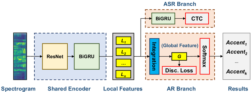
Figure 1: The Proposed Deep Accent Recognition Network

2.1 Front-end Encoder

As Table 1 shows, after the input spectrogram $\mathcal{X}\in\mathbb{R}^{T\times D\times 1}$ ($T$ denotes the temporal dimension and $D$ denotes the feature dimension ) is feed into the thin 34-layers ResNet (the number of feature maps is cut in half), we obtain the feature maps $\mathcal{L}_{1}\in\mathbb{R}^{(T/2^{5})\times(D/2^{5})\times 256}$ (the ResNet has 5 pooling operations overall). Then we could deem tensor $\mathcal{L}_{1}$ as feature sequence $\mathcal{L}_{2}\in\mathbb{R}^{(T\cdot D/2^{10})\times 256}$ by combining the time dimension and feature dimension. Next, we can reduce the dimension of descriptors to $\mathcal{H}$ by linear layer and get tensor $\mathcal{L}_{3}\in\mathbb{R}^{(T\cdot D/2^{10})\times\mathcal{H}}$. Finally, we adopt BiGRU to further extract sequential feature $\mathcal{L}_{4}\in\mathbb{R}^{(T\cdot D/2^{10})\times\mathcal{H}}$. In practice, the tensor dimension is rounded up after each pooling, for the pre-pooled dimension $x$, the pooled dimension $P(x)$ is $P(x)=\lceil x/2\rceil$. So, for a variable-length input speech with $T$ frames and $D$ dimensional acoustic feature, the amount $C$ of the descriptors we can extract using the proposed encoder is calculated as follow:

$$C(T,D)=P(P(P(P(P(T)))))\cdot P(P(P(P(P(D)))))$$ (1)

Table 1: The construction of CRNN based font-end encoder

Tensor	Layer	Output Shape
$\mathcal{X}$	$Spectrogram$	$T\times$D$\times 1$
$\mathcal{L}_{1}$	$ResNet$	$(T/2^{5})\times(D/2^{5})\times 256$
$\mathcal{L}_{2}$	$Reshape$	$(T\cdot D/2^{10})\times 256$
$\mathcal{L}_{3}$	$Linear$	$(T\cdot D/2^{10})\times\mathcal{H}$
$\mathcal{L}_{4}$	$BiGRU$	$(T\cdot D/2^{10})\times\mathcal{H}$

2.2 Many-to-One Feature Integration

It’s a crucial link to merge the variable number of local descriptors caused by the variable-length input into a fixed-length utterance-level embedding vector, that is, we have to transform local descriptors $\mathcal{L}_{4}$ extracted in subsection 2.1 into global vector $\mathcal{G}\in\mathbb{R}^{\mathcal{H}}$. In this paper, we employ RNN based integration, concretely, we use BiGRU to ingest each descriptor step by step and calculate the last hidden state as an integration result.

2.3 CTC-based ASR Objective

Here, we select CTC-based ASR [26] secondary task to curb overfitting during training. CTC formulation uses L-length letter sequence $O=\{o_{l}\in\mathcal{U}|l=1,\dots,L\}$ ($\mathcal{U}$ is vocabulary), and framewise letter sequence with ’blank’ ($<b>$) symbol: $Z=\{z_{t}\in\mathcal{U}\cup<b>|t=1,\dots T^{{}^{\prime}}\}$. According to the probabilistic chain rule and conditional independence assumption, for the input $\mathcal{X}$, the CTC objective $p_{ctc}(O|\mathcal{X})$ is factorized as follows:

$$p_{ctc}(O|\mathcal{X})=\sum_{Z}\prod_{t}p(z_{t}|z_{t-1},O)p(z_{t}|\mathcal{X})$$ (2)

where $p(z_{t}|z_{t-1},O)$ is transition probability and $p(z_{t}|\mathcal{X})$ is framewise posterior distribution. In our work, the probability $p(z_{t}|\mathcal{X})$ can be modeled by BiGRU:

$$p(z_{t}|\mathcal{X})=Softmax(Lin(h_{t}))$$ (3)

$$h_{t}=BiGRU_{asr}^{t}(Encoder(\mathcal{X}))$$ (4)

where $Softmax(\cdot)$ is a softmax activation, $Lin(\cdot)$ is a liner layer to convert $\mathcal{H}$ dimensional hidden vector to $(|\mathcal{U}|+1)$ dimensional posterior vector, $Encoder(\cdot)$ is shared front-end extractor and $BiGRU_{asr}^{t}(\cdot)$ accepts all shared local descriptors and outputs hidden vector at $t$ in ASR branch.

3 Discriminative Feature Learning

Loss function plays an important role in deep feature learning. Here, we adopt the powerful discriminative losses in FR works to improve the ambiguous accent representation.

3.1 Softmax Loss

Softmax loss, a complex of softmax function and cross entropy loss, is dedicated to making all categories have the largest log likelihood in the probability space. Given an utterance-level accent feature $\mathcal{G}_{i}$ with its corresponding label $y_{i}$, the softmax loss can be formulated as Equation 5:

$$\mathcal{L} =\frac{1}{N}\sum_{i}-log\frac{e^{W_{y_{i}}^{T}\mathcal{G}_{i}}}{\sum_{k}e^{W_{k}^{T}\mathcal{G}_{i}}}$$ (5)

$$=\frac{1}{N}\sum_{i}-log\frac{e^{\|W_{y_{i}}\|\|\mathcal{G}_{i}\|cos(\theta_{y_{i},i})}}{\sum_{k}e^{\|W_{k}\|\|\mathcal{G}_{i}\|cos(\theta_{k,i})}}$$

where $N$ denotes the batch size, $W_{k}$ refers to the $k$-th class weight vector and $\theta_{j,i}$ is the angle between $W_{j}$ and $\mathcal{G}_{i}$. But the features trained by this loss is often not good enough for the threshold-based tasks (such as retrieval and verification), that is, the correct classification does not mean obtaining a metric space with good generalization.

3.2 CosFace/AM-Softmax

In discriminative optimization, we need a reliable metric space, maximizing inter-class variance and minimizing intra-class variance, to improve the generalization in prediction, which is not the target optimized by the Softmax loss function. [20] and [21] reformulate the Softmax loss as a cosine loss by L2 normalizing both features and weight vectors to remove radial variations, based on that, an additive cosine margin term is introduced to further maximize the decision margin in the angular space:

$$\mathcal{L}=\frac{1}{N}\sum_{i}-log\frac{e^{\gamma\cdot(cos(\theta_{y_{i},i})-m)}}{e^{\gamma\cdot(cos(\theta_{y_{i},i})-m)}+\sum_{k\neq y_{i}}e^{cos(\theta_{k,i})}}$$ (6)

where hyper-parameters $\gamma$ and $m$ are scale factor and margin respectively.

3.3 ArcFace

As additive margin as Cosface and AM-softmax, under the normalization on class weights and embedding features, ArcFace[22] moves the margin into the internal of $cos$ operator to optimize the feature space more directly:

$$\mathcal{L}=\frac{1}{N}\sum_{i}-log\frac{e^{\gamma\cdot cos(\theta_{y_{i},i}+m)}}{e^{\gamma\cdot cos(\theta_{y_{i},i}+m)}+\sum_{k\neq y_{i}}e^{cos(\theta_{k,i})}}$$ (7)

3.4 Circle-Loss

[23] proposes a unified perspective in the deep feature learning including two elemental paradigms: learning with class-level labels [20, 21, 22] and learning with pair-wise labels [27, 28], which are both aiming to maximize the intra-class similarity $s_{p}$ and minimize the inter-class similarity $s_{n}$, concretely, seek to reduce ($s_{n}-s_{p}$). Given embedding accent feature $\mathcal{G}$ in the feature space, we assume that there are $K$ intra-class similarity scores and $L$ inter-class similarity scores associated with $\mathcal{G}$. We denote these similarity scores as $\{s_{p}^{i}\}(i=1,2,\cdots,K)$ and $\{s_{n}^{j}\}(j=1,2,\cdots,L)$, respectively. A unified loss function can formulated as:

$$\mathcal{L}_{uni} =log[1+\sum_{i=1}^{K}\sum_{j=1}^{L}e^{\gamma(s_{n}^{j}-s_{p}^{i}+m)}]$$ (8)

$$=log[1+\sum_{j=1}^{L}e^{\gamma(s_{n}^{j}+m)}\sum_{i=1}^{K}e^{\gamma(-s_{p}^{i})}]$$

in which $\gamma$ is a scale factor and $m$ is a margin used for similarity separation. Owing to lacking flexible optimization and ambiguous convergence status in the previous loss functions in reducing ($s_{n}-s_{p}$) process, [23] proposed Circle-Loss function:

$$\mathcal{L}_{circle} =log[1+\sum_{j=1}^{L}e^{\gamma\alpha_{n}^{j}(s_{n}^{j}-\Delta_{n})}\sum_{i=1}^{K}e^{-\gamma\alpha_{p}^{i}(s_{p}^{i}-\Delta_{p})}]$$ (9)

where $\Delta_{n}$ and $\Delta_{p}$ are the special margin for $s_{n}^{j}$ and $s_{p}^{i}$ respectively due to their asymmetric positions. According to Equation 9, Equation 10 generalizes $(s_{n}^{j}-s_{p}^{i})$ into $(\alpha_{n}^{j}s_{n}^{j}-\alpha_{p}^{i}s_{p}^{i})$, $\alpha_{n}^{j}$ and $\alpha_{p}^{j}$ are self-paced weights during inconsistent gradient descents:

$$\left\{\begin{matrix}\alpha_{p}^{i}=[O_{p}-s_{p}^{i}]+,\\ \alpha_{n}^{j}=[s_{n}^{j}-O_{n}]+,\end{matrix}\right.$$ (10)

in which $O_{n}$ and $O_{p}$ are the optimum for $s_{n}^{j}$ and $s_{p}^{j}$ respectively, $[\cdot]+$ is the $relu$ activation. Further, Circle-Loss simplifies its hyper-parameters by setting $O_{p}=1+m$, $O_{n}=-m$, $\Delta_{p}=1-m$ and $\Delta_{n}=m$ with a single margin $m$.

4 Experiment

4.1 Dataset

We trained and tested our network on the AESRC2020 speech data-set [8], an 160 hours open accented English corpus composed of train-set, development-set (dev-set) and test-set for the challenge in accent recognition (track1) and accented speech recognition (track2) with eight national level accents: Chinese (CHN), Indian (IND), Japanese (JPN), Korean (KR), American (US), British (UK), Portuguese (PT), and Russian (RU). Simultaneously, the labels including the accent of the speaker and speech transcript were offered. The detailed distribution of utterances/speakers (U/S) per national accent was exhibited in Table 2. Additionally, the open data-set without accent labels, Librispeech [29], was allowed to be used in AESRC2020.

Table 2: The detailed distribution of utterances and speakers on the 160 hours data-set of AESRC2020

Data	U/S (CHN)	U/S (IND)	U/S (JAP)	U/S (KR)	U/S (US)	U/S (UK)	U/S (PT)	U/S (RU)
train-set	13583/46	13352/38	15297/42	15807/41	16885/64	17772/83	16343/48	14945/37
dev-set	1490/4	1313/4	1488/4	1845/4	1426/4	1751/4	1616/4	1616/4
test-set	1863/-	1731/-	1794/-	1810/-	2200/-	1567/-	1819/-	1709/-

4.2 Baseline

With Fbank input-feature, the AESRC2020 provided a comparable baseline system realized on EspNet [30], and composed of the transformer [31] based encoder and Specaugment [32] preprocessing. They integrate temporal descriptors using statistical pooling [11]. Additionally, for the overfitting issue, the baseline proposed to initiate the weights of the encoder using a trained ASR encoder-decoder model (ASR-Init.), as a result, the classification accuracy improved significantly.

4.3 Training

We built and trained our model using Keras [33]. In batch training, we extracted 80-dim Fbank acoustic feature and fixed the maxlength of input frames with 1200, according to Equation 1, we obtained 114 local descriptors finally. Our CTC-based objective adopted BPE [34] based 1000 subwords and we pre-trained a CTC-based ASR model on AESRC2020 and Librispeech data-set. We restricted the dimension $\mathcal{H}$ of descriptors to 256. We set the scale factor $\gamma$ with 30 for CosFace and ArcFace, and 256 for Circle-Loss. Our MTL loss was defined as: $L=\alpha L_{ctc}+(1-\alpha)L_{disc.}+\beta L_{classifier}$, where we assigned $\alpha$ and $\beta$ with 0.4 and 0.01 respectively (We assigned $\beta$ a small value to reduce the impact of softmax classifier on feature space). Additionally, We adopted Adam optimizer [35] and set initial learning rate with 0.01. We executed early-stopping and automatic learning decay trick (the decay factor was 0.3) where the monitor was the accuracy in dev-set.

4.4 Results

Table 3 gave the detailed configurations and the accuracy for ours and the baseline. Firstly, without ASR-Init., the baseline systems and our models were both seriously over-fitted, but our accuracy could be improved greatly by adding CTC objective. Next, we compared the scores under the ASR-Init., obviously, the overfitting was improved significantly. Surprisingly, adding CTC objective still possessed a small improvement. In our analysis, the ASR-Init. offered a good starting and MTL maintained the constraint effect throughout the training process. Then, we compared Softmax loss with discriminative losses (with different margin (m)): CosFace, ArcFace and Circle-Loss. Clearly, the accuracy under discriminative losses was higher than the accuracy under Softmax, and those discriminative results also exceeded the baseline system, among these losses, Circle-Loss with m=0.2 obtained the best result of 68.8% in the test-set.

Table 3: The results of the baseline, proposed network on the accent classification track of AESRC2020

Exp	PreProc.	Front-end Encoder	ASR Branch	Integration	Disc. Loss	Dev(%)	Test(%)
No ASR-Init.
Baseline	Specaugment	Transformer-3L	-	Statistical Pooling	Softmax	54.1	-
Baseline	Specaugment	Transformer-6L	-	Statistical Pooling	Softmax	52.2	-
Baseline	Specaugment	Transformer-12L	-	Statistical Pooling	Softmax	47.8	33.0
Ours	-	ResNet-34 + BiGRU	-	BiGRU	Softmax	56.2·	39.0
Ours	-	ResNet-34 + BiGRU	CTC	BiGRU	Softmax	68.5	52.7
ASR-Init.
Baseline	Specaugment	Transformer-12L	-	Statistical Pooling	Softmax	76.1	64.9
Ours	-	ResNet-34 + BiGRU	-	BiGRU	Softmax	74.8	61.4
Ours	-	ResNet-34 + BiGRU	CTC	BiGRU	Softmax	77.3	63.9
Ours	-	ResNet-34 + BiGRU	CTC	BiGRU	CosFace(m=0.1)	79.0	65.4
Ours	-	ResNet-34 + BiGRU	CTC	BiGRU	CosFace(m=0.2)	80.3	66.7
Ours	-	ResNet-34 + BiGRU	CTC	BiGRU	CosFace(m=0.3)	79.3	66.6
Ours	-	ResNet-34 + BiGRU	CTC	BiGRU	ArcFace(m=0.1)	78.6	65.4
Ours	-	ResNet-34 + BiGRU	CTC	BiGRU	ArcFace(m=0.2)	79.4	66.7
Ours	-	ResNet-34 + BiGRU	CTC	BiGRU	ArcFace(m=0.3)	80.2	66.5
Ours	-	ResNet-34 + BiGRU	CTC	BiGRU	Circle-Loss(m=0.1)	81.5	68.0
Ours	-	ResNet-34 + BiGRU	CTC	BiGRU	Circle-Loss(m=0.2)	81.7	68.8
Ours	-	ResNet-34 + BiGRU	CTC	BiGRU	Circle-Loss(m=0.3)	81.1	68.2

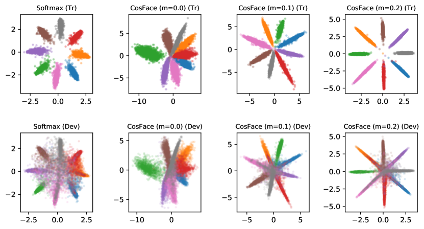
Figure 2: 2D embedding accent features trained by Softmax and CosFace (with m= 0.0, 0.1, 0.2) loss functions.

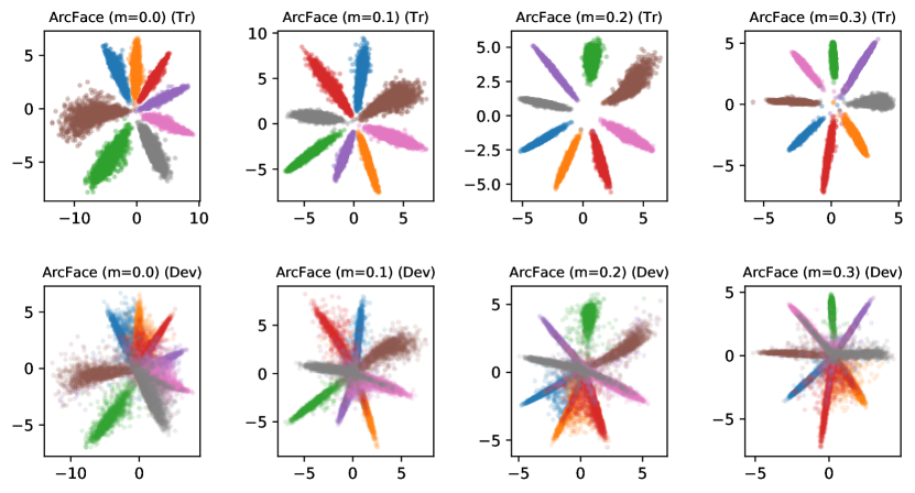
Figure 3: 2D embedding accent features trained by ArcFace (with m= 0.0, 0.1, 0.2, 0.3) loss functions.

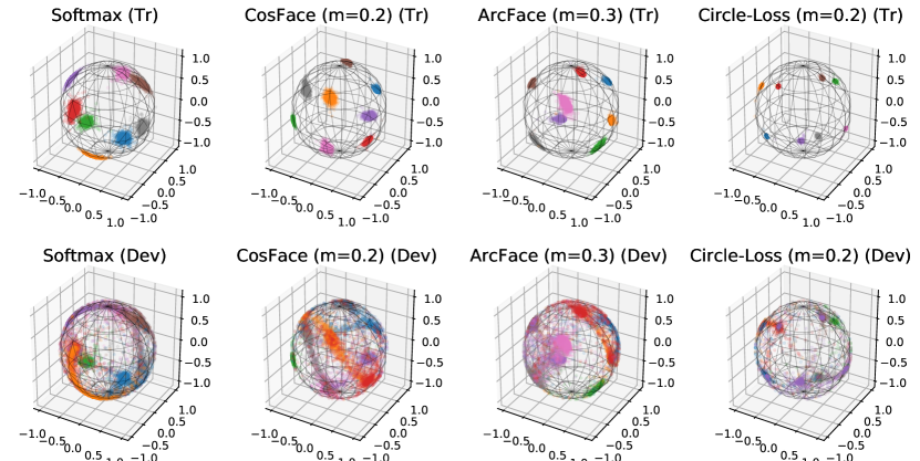
Figure 4: 3D embedding unit accent features trained by Softmax, CosFace (with m=0.2), ArcFace (with m=0.3) and Circle-Loss (with m=0.2) loss functions.

In order to better explain the discriminative learning effect, we provided a visual interpretation in low-dimensional feature space, that was, we compacted the embedding accent feature $\mathcal{G}$ into 2D/3D bottleneck feature. Figure 2 and Figure 3 showed the 2D accent feature distributions of Softmax, CosFace and ArcFace, different colors indicated different regional accents and the first row recorded the train-set and the second row recorded the dev-set, we could observe that Softmax based feature learning led to many ambiguous representations in dev-set, on the contrary, CosFace and ArcFace tightened each category features into a compact space, with the increasing of cosine/angular margin, the compact effect became more significant and we could see a more distinguishable feature distribution in dev-set. Figure 4 showed the 3D normalized accent feature distributions of Softmax, CosFace, ArcFace and Circle-Loss. Among those losses, Circle-loss made features more compact due to its improved method for flexible optimization and definite convergence status.

5 Conclusions

In this paper, we borrow the deep paradigm in speaker identification works to propose a deep accent recognition network. Novelly, we employ CTC-based ASR auxiliary task to solve overfitting problem and follow the development of discriminative feature learning in face recognition area to solve ambiguous accent representation. In the AESRC2020 accent recognition track, our proposed models with discriminative optimization both have achieved better scores than the baseline system, and Circle-Loss performs best in the feature learning. Convincingly, some preprocessings [9] achieve miraculous scores in AESRC2020, we hope to research with that and explore better scheme for accent recognition in future work.

References

- [1] Y. Ma, M. Paulraj, S. Yaacob, A. B. Shahriman, and S. K. Nataraj, “Speaker accent recognition through statistical descriptors of mel-bands spectral energy and neural network model,” in 2012 IEEE Conference on Sustainable Utilization and Development in Engineering and Technology (STUDENT). IEEE, Conference Proceedings, pp. 262–267.
- [2] F. Biadsy, “Automatic dialect and accent recognition and its application to speech recognition,” Ph.D. dissertation, Columbia University, 2011.
- [3] M. Najafian and M. Russell, “Automatic accent identification as an analytical tool for accent robust automatic speech recognition,” Speech Communication, vol. 122, pp. 44–55, 2020.
- [4] C. Teixeira, I. Trancoso, and A. Serralheiro, “Accent identification,” in Proceeding of Fourth International Conference on Spoken Language Processing. ICSLP’96, vol. 3. IEEE, 1996, pp. 1784–1787.
- [5] S. Deshpande, S. Chikkerur, and V. Govindaraju, “Accent classification in speech,” in Fourth IEEE Workshop on Automatic Identification Advanced Technologies (AutoID’05). IEEE, 2005, pp. 139–143.
- [6] A. Ahmed, P. Tangri, A. Panda, D. Ramani, and S. Karmakar, “Vfnet: A convolutional architecture for accent classification,” in 2019 IEEE 16th India Council International Conference (INDICON). IEEE, 2019, pp. 1–4.
- [7] G. I. Winata, S. Cahyawijaya, Z. Liu, Z. Lin, A. Madotto, P. Xu, and P. Fung, “Learning fast adaptation on cross-accented speech recognition,” arXiv preprint arXiv:2003.01901, 2020.
- [8] X. Shi, F. Yu, Y. Lu, Y. Liang, Q. Feng, D. Wang, Y. Qian, and L. Xie, “The accented english speech recognition challenge 2020: open datasets, tracks, baselines, results and methods,” arXiv preprint arXiv:2102.10233, 2021.
- [9] H. Huang, X. Xiang, Y. Yang, R. Ma, and Y. Qian, “Aispeech-sjtu accent identification system for the accented english speech recognition challenge,” arXiv preprint arXiv:2102.09828, 2021.
- [10] K. Okabe, T. Koshinaka, and K. Shinoda, “Attentive statistics pooling for deep speaker embedding,” arXiv preprint arXiv:1803.10963, 2018.
- [11] S. Shon, H. Tang, and J. Glass, “Frame-level speaker embeddings for text-independent speaker recognition and analysis of end-to-end model,” in 2018 IEEE Spoken Language Technology Workshop (SLT). IEEE, 2018, pp. 1007–1013.
- [12] W. Xie, A. Nagrani, J. S. Chung, and A. Zisserman, “Utterance-level aggregation for speaker recognition in the wild,” in ICASSP 2019-2019 IEEE International Conference on Acoustics, Speech and Signal Processing (ICASSP). IEEE, 2019, pp. 5791–5795.
- [13] A. Nagrani, J. S. Chung, W. Xie, and A. Zisserman, “Voxceleb: Large-scale speaker verification in the wild,” Computer Speech & Language, vol. 60, p. 101027, 2020.
- [14] P. Rangan, S. Teki, and H. Misra, “Exploiting spectral augmentation for code-switched spoken language identification,” arXiv preprint arXiv:2010.07130, 2020.
- [15] N. E. Safitri, A. Zahra, and M. Adriani, “Spoken language identification with phonotactics methods on minangkabau, sundanese, and javanese languages,” Procedia Computer Science, vol. 81, pp. 182–187, 2016.
- [16] C. Madhu, A. George, and L. Mary, “Automatic language identification for seven indian languages using higher level features,” in 2017 IEEE International Conference on Signal Processing, Informatics, Communication and Energy Systems (SPICES). IEEE, 2017, pp. 1–6.
- [17] B. Shi, X. Bai, and C. Yao, “An end-to-end trainable neural network for image-based sequence recognition and its application to scene text recognition,” IEEE transactions on pattern analysis and machine intelligence, vol. 39, no. 11, pp. 2298–2304, 2016.
- [18] K. He, X. Zhang, S. Ren, and J. Sun, “Deep residual learning for image recognition,” in Proceedings of the IEEE conference on computer vision and pattern recognition, 2016, pp. 770–778.
- [19] J. Chung, C. Gulcehre, K. Cho, and Y. Bengio, “Empirical evaluation of gated recurrent neural networks on sequence modeling,” arXiv preprint arXiv:1412.3555, 2014.
- [20] F. Wang, J. Cheng, W. Liu, and H. Liu, “Additive margin softmax for face verification,” IEEE Signal Processing Letters, vol. 25, no. 7, pp. 926–930, 2018.
- [21] H. Wang, Y. Wang, Z. Zhou, X. Ji, D. Gong, J. Zhou, Z. Li, and W. Liu, “Cosface: Large margin cosine loss for deep face recognition,” in Proceedings of the IEEE conference on computer vision and pattern recognition, 2018, pp. 5265–5274.
- [22] J. Deng, J. Guo, N. Xue, and S. Zafeiriou, “Arcface: Additive angular margin loss for deep face recognition,” in Proceedings of the IEEE/CVF Conference on Computer Vision and Pattern Recognition, 2019, pp. 4690–4699.
- [23] Y. Sun, C. Cheng, Y. Zhang, C. Zhang, L. Zheng, Z. Wang, and Y. Wei, “Circle loss: A unified perspective of pair similarity optimization,” in Proceedings of the IEEE/CVF Conference on Computer Vision and Pattern Recognition, 2020, pp. 6398–6407.
- [24] W. Cai, J. Chen, and M. Li, “Exploring the encoding layer and loss function in end-to-end speaker and language recognition system,” arXiv preprint arXiv:1804.05160, 2018.
- [25] C. Li, X. Ma, B. Jiang, X. Li, X. Zhang, X. Liu, Y. Cao, A. Kannan, and Z. Zhu, “Deep speaker: an end-to-end neural speaker embedding system,” arXiv preprint arXiv:1705.02304, vol. 650, 2017.
- [26] S. Watanabe, T. Hori, S. Kim, J. R. Hershey, and T. Hayashi, “Hybrid ctc/attention architecture for end-to-end speech recognition,” IEEE Journal of Selected Topics in Signal Processing, vol. 11, no. 8, pp. 1240–1253, 2017.
- [27] E. Hoffer and N. Ailon, “Deep metric learning using triplet network,” in International workshop on similarity-based pattern recognition. Springer, 2015, pp. 84–92.
- [28] F. Schroff, D. Kalenichenko, and J. Philbin, “Facenet: A unified embedding for face recognition and clustering,” in Proceedings of the IEEE conference on computer vision and pattern recognition, 2015, pp. 815–823.
- [29] V. Panayotov, G. Chen, D. Povey, and S. Khudanpur, “Librispeech: an asr corpus based on public domain audio books,” in 2015 IEEE international conference on acoustics, speech and signal processing (ICASSP). IEEE, 2015, pp. 5206–5210.
- [30] S. Watanabe, T. Hori, S. Karita, T. Hayashi, J. Nishitoba, Y. Unno, N. E. Y. Soplin, J. Heymann, M. Wiesner, N. Chen et al., “Espnet: End-to-end speech processing toolkit,” arXiv preprint arXiv:1804.00015, 2018.
- [31] A. Vaswani, N. Shazeer, N. Parmar, J. Uszkoreit, L. Jones, A. N. Gomez, L. Kaiser, and I. Polosukhin, “Attention is all you need,” arXiv preprint arXiv:1706.03762, 2017.
- [32] D. S. Park, W. Chan, Y. Zhang, C.-C. Chiu, B. Zoph, E. D. Cubuk, and Q. V. Le, “Specaugment: A simple data augmentation method for automatic speech recognition,” arXiv preprint arXiv:1904.08779, 2019.
- [33] A. Gulli and S. Pal, Deep learning with Keras. Packt Publishing Ltd, 2017.
- [34] R. Sennrich, B. Haddow, and A. Birch, “Neural machine translation of rare words with subword units,” arXiv preprint arXiv:1508.07909, 2015.
- [35] D. P. Kingma and J. Ba, “Adam: A method for stochastic optimization,” arXiv preprint arXiv:1412.6980, 2014.