Revealing the Accretion Physics of Supermassive Black Holes at Redshift $z\sim 7$ with Chandra and Infrared Observations

Abstract

X-ray emission from quasars has been detected up to redshift $z=7.5$, although only limited to a few objects at $z>6.5$. In this work, we present new Chandra observations of five $z>6.5$ quasars. By combining with archival Chandra observations of six additional $z>6.5$ quasars, we perform a systematic analysis on the X-ray properties of these earliest accreting supermassive black holes (SMBHs). We measure the black hole masses, bolometric luminosities ($L_{\rm bol}$), Eddington ratios ($\lambda_{\rm Edd}$), emission line properties, and infrared luminosities ($L_{\rm IR}$) of these quasars using infrared and sub-millimeter observations. Correlation analysis indicates that the X-ray bolometric correction (the factor that converts from X-ray luminosity to bolometric luminosity) decreases with increasing $L_{\rm bol}$, and that the UV/optical-to-X-ray ratio, $\alpha_{\rm ox}$, strongly correlates with $L_{\rm 2500\AA}$, and moderately correlates with $\lambda_{\rm Edd}$ and blueshift of C iv emission lines. These correlations are consistent with those found in lower-$z$ quasars, indicating quasar accretion physics does not evolve with redshift. We also find that $L_{\rm IR}$ does not correlate with $L_{\rm 2-10keV}$ in these luminous distant quasars, suggesting that the ratio of the SMBH growth rate and their host galaxy growth rate in these early luminous quasars are different from those of local galaxies. A joint spectral analysis of the X-ray detected $z>6.5$ quasars yields an average X-ray photon index of $\Gamma=2.32^{+0.31}_{-0.30}$, steeper than that of low-$z$ quasars. By comparing it with the $\Gamma-\lambda_{\rm Edd}$ relation, we conclude that the steepening of $\Gamma$ for quasars at $z>6.5$ is mainly driven by their higher Eddington ratios.

1 Introduction

Quasars, the most luminous type of active galactic nuclei (AGN), are believed to be powered by accreting supermassive black holes (SMBHs). The continuum and line emission from luminous quasars, over a large wavelength range, from optical to X-ray, can be characterized by several major components: the optical-to-ultraviolet (UV) continuum emission which is explained by a standard accretion disk extending down to the innermost stable circular orbit (ISCO; e.g. Shields, 1978), a soft X-ray excess whose origin is still debated (e.g. Arnaud et al., 1985), X-ray emission with a power-law spectrum produced by inverse Compton scattering of photons from the accretion disk of relativistic electrons in the hot corona (e.g. Svensson & Zdziarski, 1994), and the broad emission lines emitted from the so-called broad line region (BLR; e.g. Antonucci, 1993). Thus the optical/UV to X-ray emission of quasars provide crucial information about the BH mass, the structure and physics of the accretion flow around the central SMBHs.

At present more than 200 quasars have been discovered at redshift $z>6$ (e.g. Fan et al., 2001; Wu et al., 2015; Jiang et al., 2016; Bañados et al., 2016; Wang et al., 2017; Reed et al., 2017; Yang et al., 2017); about 50 quasars have been discovered at $z>6.5$ (e.g. Venemans et al., 2013; Wang et al., 2019b; Mazzucchelli et al., 2017; Yang et al., 2019) and seven at $z>7$ (Mortlock et al., 2011; Bañados et al., 2018a; Wang et al., 2018; Matsuoka et al., 2019; Yang et al., 2019, 2020). Extensive optical to near-infrared (NIR) spectroscopic observations of these quasars indicate that billion solar mass SMBHs are already in place when the universe is only $\sim$700 Myrs old (Yang et al., 2020). The growth of these early SMBHs is limited by the available accretion time. At $z\sim 7$, only $\sim 14$ $e$-folding times elapsed since the first luminous object formed in the Universe (i.e. $z\sim 30$, Tegmark et al., 1997), corresponding to a factor of $\sim 10^{6}$ increase in mass, placing the most stringent constraints on the SMBH formation and growth mechanisms (e.g. Bañados et al., 2018a; Yang et al., 2020). In order to explain the existence of these SMBHs, many theoretical models have been proposed (see Latif & Ferrara, 2016; Inayoshi et al., 2019, and references therein) by invoking either super-Eddington accretion process (e.g., Volonteri et al., 2015) and/or a massive seed BH (e.g., Omukai et al., 2008; Volonteri et al., 2008; Wise et al., 2019).

The X-ray emission from quasars carries crucial information about the accretion physics and AGN feedback (e.g. Fabian et al., 2014; Parker et al., 2017). However, X-ray observations are only available for a very limited sample at high redshift. To date, $\sim$30 $z\sim$6 quasars (e.g., Brandt et al., 2001; Shemmer et al., 2006; Ai et al., 2016, 2017; Nanni et al., 2017, 2018; Vito et al., 2019; Connor et al., 2019) and six $z>6.5$ quasars (Page et al., 2014; Moretti et al., 2014; Bañados et al., 2018b; Vito et al., 2019; Pons et al., 2020; Connor et al., 2020) have been detected in X-ray with Chandra and XMM-Newton. Two key findings have been established based on these limited X-ray observations.

Table 1: Basic properties and observations for $z>6.5$ quasars

Name	Ra	Dec	$z$	$J_{\rm AB}$	obs. date	ObsID	Mode	${t_{\rm exp,X}}$	NIR Inst.	${t_{\rm exp,NIR}}$	$N_{\rm H}$	Ref. (disc./$z$)
					yyyy-mm-dd			[ks]		[ks]	[$10^{20}$ cm-2]
J2348$-$3054	23:48:33.34	$-$30:54:10.0	6.9018	21.11$\pm$0.11	2018-09-04	20414	VFAINT	42.50	X-Shooter	9.2	1.30	V13/V16
J1048$-$0109	10:48:19.09	$-$01:09:40.2	6.6759	20.61$\pm$0.17	2019-01-28	20415	VFAINT	34.76	X-Shooter	4.8	3.60	W17/D18
J0024$+$3913	00:24:29.77	$+$39:13:19.0	6.6210	20.70$\pm$0.15	2018-05-21	20416	VFAINT	19.70	GNIRS	13.8	6.76	T17/M17
J2132$+$1217	21:32:33.19	$+$12:17:55.3	6.5850	19.55$\pm$0.11	2018-08-20	20417	VFAINT	17.82	X-Shooter	8.4	6.42	M17/D18
J0224$-$4711	02:24:26.54	$-$47:11:29.4	6.5223	19.73$\pm$0.06	2018-03-05	20418	VFAINT	17.72	X-Shooter	4.8	1.66	R17/W20
J1342$+$0928	13:42:08.11	$+$09:28:38.6	7.5413	20.36$\pm$0.10	2017-12-15	20124	VFAINT	24.73	GNIRS	32.4	2.04	B18/V17
					2017-12-17	20887	VFAINT	20.38
J1120$+$0641	11:20:01.48	$+$06:41:24.3	7.0842	20.30$\pm$0.15	2011-02-04	13203	FAINT	15.84	GNIRS	4.8	5.07	M11/D18
J2232$+$2930	22:32:55.15	$+$29:30:32.0	6.6580	20.28$\pm$0.14	2018-01-30	20395	VFAINT	54.21	GNIRS	4.8	6.71	V15/D18
J0305$-$3150	03:05:16.92	$-$31:50:56.0	6.6145	20.70$\pm$0.09	2018-05-11	20394	VFAINT	49.88	X-Shooter	16.8	1.42	V13/V16
J0226$+$0302	02:26:01.87	$+$03:02:59.3	6.5412	19.43$\pm$0.10	2018-10-09	20390	VFAINT	25.90	X-Shooter	4.8	3.04	V15/B15
J1110$-$1329	11:10:33.96	$-$13:29:45.6	6.5148	21.16$\pm$0.09	2018-02-20	20397	VFAINT	59.33	FIRE	12.0	5.31	V15/D18

Note. — The first section includes five quasars with new Chandra observations, while the second section represents six quasars with archival X-ray observations. All redshift comes from the fitting of [C ii] emission line. The sources are sorted by decreasing redshift.

References: B15: Bañados et al. (2015); B18: Bañados et al. (2018b); D18: Decarli et al. (2018); M17: Mazzucchelli et al. (2017); R17: Reed et al. (2017); T17: Tang et al. (2017); V13: Venemans et al. (2013); V16: Venemans et al. (2016) W20: The [C ii] redshift of this object is obtained from ALMA Cycle 6 observations (2018.1.01188.S, PI: Wang) (Wang et al. in preparation).

First, there is a tight correlation between the optical/UV-X-ray luminosity ratio ($\alpha_{\rm ox}$) and the UV luminosity (i.e. $L_{\rm 2500\AA}$), and it does not evolve from low redshift up to $z\sim 6$ (e.g. Just et al., 2007; Lusso & Risaliti, 2016; Nanni et al., 2017). Recent investigations of several $z>6.5$ quasars (Moretti et al., 2014; Page et al., 2014; Bañados et al., 2018a; Vito et al., 2019) suggest that this relation might still hold in the epoch of reionization. Since $\alpha_{\rm ox}$ measures the relative importance of the hot corona versus the accretion disk, the steeper $\alpha_{\rm ox}$ in higher luminosity quasars indicates the dominance of the disk emission with respect to the hot electron corona emission in luminous quasars (see Brandt & Alexander, 2015, for a review).

The other key finding is that there is a moderate positive correlation between the photon index, $\Gamma$, of the hard X-ray spectrum ($N(E)\propto E^{-\Gamma}$) and the Eddington ratio ($\lambda_{\rm Edd}=L/L_{\rm Edd}$) established from a sizable sample of sources up to $z\sim 3$, with larger $\Gamma$ corresponding to higher $\lambda_{\rm Edd}$ (e.g. Shemmer et al., 2008; Brightman et al., 2013, but see Trakhtenbrot et al. (2017)). A high accretion rate is expected to increase the disk temperature and thus the level of disk emission, resulting in the increase of Compton cooling of the corona (e.g., Maraschi & Haardt, 1997), and producing a steep (large $\Gamma$) X-ray spectrum. However, the relation between $\Gamma$ and $\lambda_{\rm Edd}$ is far from well established for the most distant quasars. Measuring $\Gamma$ is extremely difficult at high redshift because of the limited photon statistics. To date, only for four quasars (three at $z\sim 6$ quasars and one at $z>7$) have more than 100 X-ray  photons been detected, which is required to place reasonable constraints on $\Gamma$ for individual quasars (Page et al., 2014; Moretti et al., 2014; Ai et al., 2017; Nanni et al., 2017, 2018). Alternatively, stacking studies of quasars to study the average $\Gamma$ at differents redshifts indicates that the average $\Gamma$ does not evolve from $z\sim 0$ to $z\sim 6$ (Just et al., 2007; Vignali et al., 2005; Shemmer et al., 2006; Nanni et al., 2017). However, the more recent work by Vito et al. (2019) indicates that the average $\Gamma$ of three $z>6.5$ quasars is slightly steeper than but still consistent with those of typical quasars at $z<6$.

In this paper, we report new Chandra observations of five quasars at $z>6.5$, significantly increasing the number of X-ray observed quasars at these redshifts. Together with archival Chandra observations of six additional $z>6.5$ quasars, we perform joint spectral fitting of all X-ray detected $z>6.5$ quasars with a mean quasar redshift of $z=6.822$. We also analyze the NIR spectra for these quasars and investigate the relations between quasar rest-frame UV and X-ray properties. In Section 2 we describe the X-ray and NIR observations and data reduction. We present the X-ray fluxes, luminosities, $\alpha_{\rm ox}$ measurements from Chandra observations, the black hole masses, bolometric luminosities, Eddington ratios and line properties measurements from NIR spectral fitting, and the infrared luminosities measured from sub-millimeter observations in Section 3. The correlation between X-ray and other properties of individual quasars are investigated in Section 4. We present the stacked X-ray spectrum, joint spectral fitting, and the mean properties of these $z>6.5$ quasars in Section 5. Finally, we conclude and summarize our findings in Section 6. Throughout the paper, we adopt a flat cosmological model with $H_{0}=68.5~{}{\rm km~{}s^{-1}~{}Mpc^{-1}}$ (Betoule et al., 2014), $\rm\Omega_{M}=0.3$, and $\Omega_{\Lambda}=0.7$. All the uncertainties of our measurements reported in this work are at 1-$\sigma$ confidence level, while upper limits are reported at the 95% confidence level.

2 Observations and Data Reduction

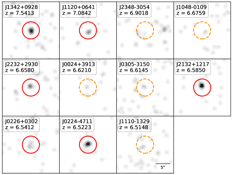
Figure 1: Full-band (0.5–7 keV) Chandra cutouts of the eleven $z>6.5$ quasars. The images are centered at the optical positions listed in Table 1. The images have been smoothed with a 1 pixel Gaussian kernel. Red solid circles highlight targets detected by wavdetect, while the orange dashed circles denote targets not detected by wavdetect. All circles represent our extraction regions with a $3.0^{\prime\prime}$ radius. All cutouts are in the size of $20^{\prime\prime}\times 20^{\prime\prime}$.

2.1 Chandra X-ray Observations

We obtained Chandra observations of five quasars at $z>6.5$ using the Advanced CCD imaging spectrometer (ACIS-S, Garmire et al., 2003) instrument in Cycle 19 (proposal number: 19700283, PI. Fan). The five quasars observed were J002429.77+391319.0 (hereafter J0024+3913, Tang et al., 2017) at $z=6.6210$, J022426.54–471129.4 (hereafter J0224–4711, Reed et al., 2017) at $z=6.5223$, J104819.09–010940.21 (hereafter J1048–0109, Wang et al., 2017) at $z=6.6759$, J213233.19+121755.3 (hereafter J2132+1217, Mazzucchelli et al., 2017) at $z=6.5850$, and J234833.34–305410.0 (hereafter J2348–3054, Venemans et al., 2013) at $z=6.9018$. These targets were positioned on the ACIS-S3 chip with the Very Faint telemetry format and the Timed Exposure mode. The observation log and the basic properties (i.e. redshift and brightness) of these quasars are listed in Table 1.

In order to increase the sample size of our analysis we also include the six other $z>6.5$ quasars that were observed by Chandra and archived as of 2020 April. Specifically, J112001.48+064124.3 (hereafter J1120+0641, Mortlock et al., 2011) at $z=7.09$ was observed in Cycle 12 (Page et al., 2014), J134208.10 +092838.6 (hereafter J1342+0928, Bañados et al., 2018b) at $z=7.54$ was observed in Cycle 18 (Bañados et al., 2018a), and four other quasars were observed in Cycle 19 (Vito et al., 2019). The observation log and properties of these quasars are also listed in Table 1. The Galactic H i column density at each quasar position calculated from Kalberla et al. (2005) is also listed in Table 1. Similar with our new observations, these $z>6.5$ quasars were positioned on the ACIS-S3 chip with the Timed Exposure mode. J1120+0641 was observed with the Faint telemetry format and all other quasars were observed with the Very Faint mode.

The data were reprocessed with the chandra_repro script in the standard Chandra’s data analysis system: CIAO (Fruscione et al., 2006) version 4.12 and CALDB version 4.9.0. In the analyses, only grade 0, 2, 3, 4, and 6 events were used. In the process, we set the option check_vf_pha = yes in the case of observations taken in very faint mode. The exposure maps and the PSF maps were created with the fluximage script and the mkpsfmap script, respectively. Considering the increasingly uncertain quantum efficiency of ACIS at lower energies and the steeply increasing background at higher energies, we only used the X-ray counts at observed frame energies of 0.5–7keV, following Nanni et al. (2017). In order to detect sources we first performed source detections using wavdetect (Freeman et al., 2002) with a false-positive probability threshold of $10^{-5}$. Six quasars were detected by wavdetect: J1342+0928, J1120+0641, J2232+2930, J2132+1217, J0226+0302, and J0224–4711, with the net counts of $14.2^{+5.0}_{-3.8}$, $5.8^{+3.6}_{-2.4}$, $7.1^{+3.9}_{-2.8}$, $15.6^{+5.1}_{-4.0}$, $5.5^{+3.6}_{-2.4}$, and $18.3^{+5.4}_{-4.3}$, respectively. The uncertainties are estimated according to the approximation of Gehrels (1986).

Table 2: X-ray photometry and quasar X-ray properties.

Name	Net Counts			HR	Flux			$L_{\rm 2-10keV}$	$\rm\alpha_{ox}$
	0.5–7.0 keV	0.5–2.0 keV	2.0–7.0 keV		0.5–7.0 keV	0.5–2.0 keV	2.0–7.0 keV	$\rm 10^{44}~{}erg~{}s^{-1}$
J1342$+$0928	$14.0^{+5.1}_{-4.0}$	$10.2^{+4.4}_{-3.3}$	$3.8^{+3.4}_{-2.2}$	$-0.46^{+0.23}_{-0.29}$	$2.97^{+1.08}_{-0.85}$	$1.56^{+0.57}_{-0.45}$	$1.41^{+0.51}_{-0.40}$	$12.80^{+4.68}_{-3.69}$	$-1.61^{+0.05}_{-0.06}$
J1120$+$0641	$5.3^{+3.6}_{-2.4}$	$3.7^{+3.2}_{-1.9}$	$1.6^{+2.6}_{-1.3}$	$-0.37^{+0.33}_{-0.47}$	$2.29^{+1.56}_{-1.04}$	$1.20^{+0.82}_{-0.54}$	$1.09^{+0.74}_{-0.49}$	$8.52^{+5.82}_{-3.83}$	$-1.66^{+0.09}_{-0.10}$
J2348$-$3054	$<8.6$	$<3.0$	$<9.7$	–	$<2.26$	$<1.19$	$<1.07$	$<7.96$	$<-1.56$
J1048$-$0109	$<4.7$	$<4.1$	$<4.0$	–	$<1.54$	$<0.81$	$<0.73$	$<5.02$	$<-1.72$
J2232$+$2930	$6.6^{+4.1}_{-2.9}$	$6.3^{+3.8}_{-2.6}$	$0.4^{+2.6}_{-1.3}$	$-0.73^{+0.07}_{-0.27}$	$1.45^{+0.90}_{-0.64}$	$0.76^{+0.47}_{-0.33}$	$0.69^{+0.43}_{-0.30}$	$4.68^{+2.89}_{-2.03}$	$-1.73^{+0.08}_{-0.09}$
J0024$+$3913	$<8.2$	$<5.9$	$<5.6$	–	$<4.93$	$<2.59$	$<2.34$	$<15.74$	$<-1.47$
J0305$-$3150	$<5.8$	$<4.2$	$<5.1$	–	$<1.31$	$<0.69$	$<0.62$	$<4.18$	$<-1.73$
J2132$+$1217	$15.0^{+5.1}_{-4.0}$	$7.5^{+3.9}_{-2.8}$	$7.5^{+3.9}_{-2.8}$	$0.00^{+0.27}_{-0.25}$	$9.93^{+3.38}_{-2.65}$	$5.22^{+1.77}_{-1.39}$	$4.71^{+1.60}_{-1.26}$	$31.32^{+10.62}_{-8.34}$	$-1.50^{+0.05}_{-0.05}$
J0226$+$0302	$5.0^{+3.6}_{-2.4}$	$3.7^{+3.2}_{-1.9}$	$1.2^{+2.6}_{-1.3}$	$-0.49^{+0.16}_{-0.51}$	$2.18^{+1.57}_{-1.05}$	$1.14^{+0.82}_{-0.55}$	$1.03^{+0.74}_{-0.49}$	$6.73^{+4.84}_{-3.25}$	$-1.81^{+0.09}_{-0.11}$
J0224$-$4711	$18.1^{+5.4}_{-4.3}$	$15.7^{+5.1}_{-4.0}$	$2.4^{+2.9}_{-1.6}$	$-0.72^{+0.12}_{-0.21}$	$11.44^{+3.41}_{-2.72}$	$6.01^{+1.79}_{-1.43}$	$5.43^{+1.62}_{-1.29}$	$35.26^{+10.5}_{-8.39}$	$-1.55^{+0.04}_{-0.05}$
J1110$-$1329	$<8.0$	$<3.0$	$<8.8$	–	$<1.58$	$<0.83$	$<0.75$	$<4.86$	$<-1.60$

are listed in Table 3. The $\rm\Delta\alpha_{ox}$ used in Figure 5 can be derived by subtracting $\rm\alpha_{ox}$ from the $\alpha_{\rm ox}-L_{\rm 2500\AA}$ relation in Timlin et al. (2020).

Note. — The sources are sorted by decreasing redshift. The last column, $\rm\alpha_{ox}$, is measured using Equation (2) and the $L_{\rm 2500\AA}$

We extract the spectrum for each object within a $3\farcs 0$ radius circular region centered at the optical position using the specextract script. We choose a background annulus centered at the optical positions with an inner radius of $10\farcs 0$ and an outer radius of $30\farcs 0$. The net X-ray counts detected in the soft band (0.5–2 keV), the hard band (2–7 keV), and the full band (0.5–7 keV) within the $3\farcs 0$ radius circular region are reported in Table 2. For undetected sources we report the 2$\sigma$ upper limits (corresponding to the 95% confidence intervals) computed from the srcflux script in CIAO. Table 2 also lists the hardness ratio ${\rm HR}=(H-S)/(H+S)$, where H and S are the net counts in the hard (2–7 keV) and soft (0.5–2.0 keV) bands, respectively. The HR for those Chandra detected quasars are estimated with the Bayesian method described by Park et al. (2006). The full band (0.5-7 keV) image stamps are shown in Figure 1.

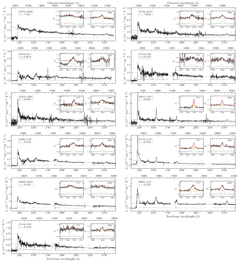
Figure 2: Near-infrared spectra of the eleven $z>6.5$ quasars studied in this paper. The spectra are re-binned to 200 $\rm km~{}s^{-1}$ pixels. The black and gray lines represent the Galactic extinction corrected spectra and one sigma error vectors. The green dashed lines denote best-fit UV power-law continuum. The left insert panels are the zoom-in of C iv line fitting, while the right insert panels are the zoom-in of Mg ii line fitting. In the insert panels, red solid lines denote total fit, green dashed lines denote power-law continuum, blue lines denote iron template, and the orange lines denote emission line components.

2.2 Near-Infrared Spectroscopy

We note that most of the quasars investigated here have BH mass estimates in the literature (Mortlock et al., 2011; De Rosa et al., 2014; Mazzucchelli et al., 2017; Bañados et al., 2018b; Tang et al., 2019; Onoue et al., 2020; Schindler et al., 2020). However, these estimates were based on different fitting algorithms and different single-epoch virial scaling relations. To reduce the biases introduced by different methods we perform our own self-consistent measurements of the masses and Eddington ratios of these SMBHs. We reduced and analyzed the archival NIR spectroscopic observations of these quasars. The quasar J1342+0928, J1120+0641, J0024+3913, and J2232+2930 were observed with Gemini/GNIRS (Elias et al., 2006a, b) using the Cross-dispersed mode. J1110–1329 was observed with Magellan/FIRE (Simcoe et al., 2010) using the Echelle mode. All the other quasars presented in this work were observed with VLT/X-Shooter (Vernet et al., 2011).

We reduced both GNIRS and X-Shooter spectra with the newly developed open source spectroscopic data reduction pipeline PyPeIt (Prochaska et al., 2020a, b). The wavelength solutions were derived from the night sky OH lines in the vacuum frame. The sky background was subtracted with the standard A–B mode and then a $b$-spline fitting procedure was performed to further clean up the sky line residuals following Bochanski et al. (2009). An optimal extraction (Horne, 1986) is then performed to generate 1D science spectra. We flux the extracted spectra with sensitivity functions derived from standard star observations. We then stacked the fluxed individual exposures and individual orders. The telluric corrections are performed by jointly fitting the atmospheric models derived from the Line-By-Line Radiative Transfer Model (LBLRTM; Clough et al., 2005) and a quasar model based on a Principal Component Analysis method (Davies et al., 2018) to the stacked quasar spectra. We then scaled the telluric corrected spectra to match the $J$-band photometry of each object by carrying out synthetic photometry on the spectrum for the purpose of absolute flux calibration. Finally, we corrected the Galactic extinction based on the dust map (Schlegel et al., 1998) and extinction law (Cardelli et al., 1989). The fully calibrated NIR spectra of these quasars are shown in Figure 2. The FIRE spectrum was reduced with the standard FIREHOSE pipeline, which evolved from the MASE pipeline for optical echelle reduction (Bochanski et al., 2009). We corrected for telluric absorption features by obtaining a spectrum of an A0V star at a comparable observing time.

3 Measurements and Results

Since all quasars have less than 20 net counts in the full 0.5-7.0 keV band, we do not attempt spectral fitting for individual quasars. We measure the X-ray flux by assuming a power-law spectrum with $\rm\Gamma=2.0$ (typical of luminous quasars, e.g., Nanni et al., 2017; Vito et al., 2019), accounting for the Galactic absorption (Kalberla et al., 2005), and using the response matrices and ancillary files extracted at the position of each target. The rest-frame 2-10 keV luminosites were estimated by assuming $\rm\Gamma=2.0$ as listed in Table 2. The measured X-ray luminosity of these quasars spans more than an order of magnitude with $L_{\rm 2-10keV}\lesssim 4-35\times 10^{44}~{}{\rm erg~{}s^{-1}}$. Note that the $L_{\rm 2-10keV}$ would be $\sim$20% higher if we use $\rm\Gamma=2.3$, the average photon index of $z>6.5$ quasars derived from §5. Considering that most previous work has used $\rm\Gamma\sim 2$ when measuring $L_{\rm 2-10keV}$ at high redshifts (e.g. Nanni et al., 2017; Vito et al., 2019), we will only use the $L_{\rm 2-10keV}$ values derived by assuming $\rm\Gamma=2$ in what follows.

To derive the rest-frame ultraviolet (UV) luminosities, black hole masses, and Eddington ratios for these quasars we performed a global spectral fitting on the de-redshifted NIR spectra following Wang et al. (2020). Briefly, we first fit a pseudo-continuum model to the emission line (except for iron emission) free regions. The pseudo-continuum model includes three components, a power-law continuum ($f_{\lambda}\propto\lambda^{\alpha_{\lambda}}$), Balmer continuum (e.g. De Rosa et al., 2014), and iron emission (Vestergaard & Wilkes, 2001; Tsuzuki et al., 2006). The iron template was constructed by composing the iron emission from Tsuzuki et al. (2006) (2200Å-3500Å) and Vestergaard & Wilkes (2001) (1100Å-2200Å). The Mg ii and C iv lines are then fitted with two Gaussian functions for each line after subtracting the pseudo-continuum model. We perform the whole fitting process iteratively and broaden the iron template by convolving it with a Gaussian kernel to match the line width of the Mg ii line. Following Wang et al. (2020), we use a Monte Carlo approach to estimate the spectral measurement uncertainties. We created 100 mock spectra by randomly adding Gaussian noise to each pixel with standard deviation equal to the spectral error at that pixel. Then we applied the exactly same fitting procedure to these mock spectra. The uncertainties of measured spectral properties are then estimated as the average of the 16% and 84% percentile deviation from the median.

The derived power-law continuum slopes ($\alpha_{\lambda}$), continuum luminosities at rest-frame 2500 Å, line widths, and redshifts are given in Table 3. The Mg ii and C iv redshifts listed in Table 3 were estimated based on the peak of the Gaussian fitting of each line. The redshifts based on the Mg ii line are in generally consistent with ($\rm<800~{}km~{}s^{-1}$) the [C ii] redshifts listed in Table 1. The C iv lines of all the quasars exhibit large blueshifts relative to both [C ii] and Mg ii lines which we discuss in detail in §4.2. The bolometric luminosities are estimated by assuming a bolometric correction of $L_{\rm bol}$=5.15$\times$ $\lambda L_{\rm 3000\text{\AA}}$ (Shen et al., 2011). The black hole masses, $M_{\rm BH}$, are then estimated using the single virial estimator proposed by Vestergaard & Osmer (2009):

$$\small\frac{M_{\rm BH}}{M_{\odot}}=10^{6.86}\left[\frac{\lambda L_{\lambda}\rm{(3000~{}\AA)}}{\rm{10^{44}~{}erg~{}s^{-1}}}\right]^{0.5}\left[\frac{\rm{FWHM_{(Mg\ II)}}}{\rm{10^{3}~{}km~{}s^{-1}}}\right]^{2}$$ (1)

The Eddington ratio of each quasar is then calculated as $\lambda_{\rm Edd}=L_{\rm bol}/L_{\rm Edd}$, where the $L_{\rm Edd}=1.26\times 10^{38}~{}M_{\rm BH}$ is the Eddington luminosity. The $M_{\rm BH}$ and $\lambda_{\rm Edd}$ are listed in Table 3. Note that the quoted uncertainties of $M_{\rm BH}$ and $\lambda_{\rm Edd}$ do not include the systematic uncertainties in the scaling relation, which is $0.55$ dex (Vestergaard & Osmer, 2009).

With the X-ray and UV luminosity, we can then measure the optical-X-ray power-law slope, which is defined as

$$\alpha_{\rm ox}=\frac{log(f_{\rm 2\>keV}/f_{\rm 2500\>\AA})}{log(\nu_{\rm 2\>keV}/\nu_{\rm 2500\>\AA})},$$ (2)

where $f_{\rm 2\>keV}$ and $f_{\rm 2500\>\AA}$ are the flux densities at rest-frame 2 keV and 2500 Å, respectively. The computed $\alpha_{\rm ox}$ values are listed in Table 2.

Table 3: Quasar properties derived from near-infrared and sub-millimeter observations.

Name	$\rm M_{1450}$	$z_{\rm MgII}$	$z_{\rm CIV}$	$\rm FWHM_{MgII}$	$\rm FWHM_{CIV}$	$\lambda L_{\rm 2500}$	$L_{\rm bol}$	$\rm M_{BH}$	$\lambda_{\rm Edd}$	$\rm S_{1mm}$	$L_{\rm IR}$	Ref. ($\rm S_{1mm}$  )
				$\rm km~{}s^{-1}$	$\rm km~{}s^{-1}$	$\rm 10^{46}~{}erg~{}s^{-1}$	$\rm 10^{47}~{}erg~{}s^{-1}$	$\rm 10^{9}~{}M_{\odot}$		mJy	$\rm 10^{46}~{}erg~{}s^{-1}$
J1342$+$0928	$-$26.65	7.531$\pm$0.004	7.361$\pm$0.025	2680$\pm$255	11776$\pm$1102	3.04$\pm$0.23	1.42$\pm$0.12	0.86$\pm$0.20	1.26$\pm$0.16	0.41$\pm$0.07	0.57$\pm$0.10	V18
J1120$+$0641	$-$26.45	7.095$\pm$0.002	7.027$\pm$0.005	3454$\pm$66	7554$\pm$690	2.80$\pm$0.24	1.35$\pm$0.11	1.40$\pm$0.10	0.74$\pm$0.06	0.53$\pm$0.04	0.73$\pm$0.06	V18
J2348$-$3054	$-$25.84	6.887$\pm$0.005	6.866$\pm$0.001	4385$\pm$786	4364$\pm$625	1.45$\pm$0.17	0.68$\pm$0.09	1.60$\pm$0.69	0.33$\pm$0.11	1.92$\pm$0.14	2.64$\pm$0.19	V18
J1048$-$0109	$-$26.03	6.661$\pm$0.005	6.603$\pm$0.015	2676$\pm$1240	10202$\pm$536	2.34$\pm$0.28	1.21$\pm$0.12	0.79$\pm$0.58	1.17$\pm$0.37	2.84$\pm$0.04	3.90$\pm$0.05	D18
J2232$+$2930	$-$26.34	6.666$\pm$0.007	6.642$\pm$0.001	5234$\pm$321	3938$\pm$215	2.35$\pm$0.40	1.11$\pm$0.19	2.91$\pm$0.57	0.29$\pm$0.02	0.97$\pm$0.22	1.33$\pm$0.30	V18
J0024$+$3913	$-$25.62	6.618$\pm$0.001	6.613$\pm$0.001	1711$\pm$139	2441$\pm$5	1.64$\pm$0.21	0.85$\pm$0.10	0.27$\pm$0.04	2.40$\pm$0.38	0.55$\pm$0.18	0.76$\pm$0.25	V18
J0305$-$3150	$-$26.11	6.608$\pm$0.002	6.576$\pm$0.003	2617$\pm$609	5624$\pm$300	2.08$\pm$0.13	1.01$\pm$0.07	0.70$\pm$0.38	1.12$\pm$0.44	3.29$\pm$0.10	4.52$\pm$0.14	V18
J2132$+$1217	$-$27.08	6.588$\pm$0.001	6.578$\pm$0.001	2146$\pm$263	3063$\pm$22	3.97$\pm$0.21	1.77$\pm$0.09	0.62$\pm$0.17	2.20$\pm$0.50	0.47$\pm$0.15	0.65$\pm$0.21	V18
J0226$+$0302	$-$27.26	6.532$\pm$0.017	6.427$\pm$0.003	3713$\pm$289	9346$\pm$1298	5.36$\pm$0.27	2.50$\pm$0.13	2.20$\pm$0.39	0.87$\pm$0.10	2.50$\pm$0.50	3.44$\pm$0.69	V18
J0224$-$4711	$-$26.67	6.527$\pm$0.001	6.486$\pm$0.001	2655$\pm$144	5760$\pm$96	5.85$\pm$0.35	3.36$\pm$0.20	1.30$\pm$0.18	1.98$\pm$0.15	1.96$\pm$0.07	2.70$\pm$0.10	W20
J1110$-$1329	$-$25.35	6.511$\pm$0.004	6.465$\pm$0.020	2267$\pm$352	13778$\pm$4155	1.10$\pm$0.14	0.55$\pm$0.06	0.38$\pm$0.14	1.10$\pm$0.24	0.87$\pm$0.05	1.20$\pm$0.07	D18

Note. — The sources are sorted by decreasing redshift.

References: D18: Decarli et al. (2018); V18: Venemans et al. (2018) W20: The 1mm continuum flux density of this object is obtained from ALMA Cycle 6 observations (2018.1.01188.S, PI: Wang) (Wang et al. in preparation).

In order to measure the infrared luminosities of these quasars we used the 1mm (in the observed frame) ALMA observations collected by Venemans et al. (2018) and Decarli et al. (2018). In addition, we observed one quasar in our sample, J0224–4711, with ALMA in Cycle 6 (2018.1.01188.S, PI: Wang). In this paper, we only use the [C ii] based redshift (Table 1) and the 1mm continuum (Table 3) measurements, while the detailed data reduction of our ALMA observations will be presented elsewhere (Wang et al. in preparation). Since Haro 11, a low metallicity dwarf galaxy, has been suggested as the best candidate analog for high-$z$ quasar host galaxies (e.g. Lyu et al., 2016), we estimate the 8–1000 $\mu$m infrared luminosities ($L_{\rm IR}$) of these quasar host galaxies by scaling the observed 1mm continuum to the Haro 11 spectral energy distribution (SED). The estimated $L_{\rm IR}$ are listed in Table 3. The star formation rate (SFR) can be calculated as

$${\rm SFR(M_{\odot}~{}yr^{-1})}=5.0\times 10^{-44}~{}L_{\rm(IR,erg~{}s^{-1})},$$ (3)

(Lyu et al., 2016). Note that the $L_{\rm IR}$ estimated using the Haro 11 template is usually about two times higher than that estimated from a modified blackbody with $T=47$ K and $\beta=1.6$ (Beelen et al., 2006), because the modified blackbody misses flux in the mid-infrared.

4 Correlations Between X-ray Emission and Other Properties of Individual Quasars

In this Section, we investigate the relationships between X-ray emission and other properties of these high redshift quasars. Since our quasar sample is relatively small and only occupies the bright end (i.e. $L_{\rm bol}\gtrsim 5\times 10^{46}~{}{\rm erg~{}s^{-1}}$) of the quasar population at very high redshift, we consider a sample of $\sim 2,000$ SDSS quasars at $1.7\leq z\leq 2.7$ that have Chandra observations (Timlin et al., 2020) to expand both sample size, luminosity range, and redshift range. We further restrict the redshift to be $z\geq 2.0$ to ensure that we have the same rest-frame UV spectral coverage as the $z>6.5$ quasars studied here; this results in a sample of 1,175 objects. We then perform exactly the same spectral fitting method used in §  3 to compute the UV luminosities, $L_{\rm bol}$, BH masses, and Eddington ratios of these lower redshift quasars. We successfully fit the Mg ii emission lines in 897 of 1,175 objects, as some SDSS spectra have very low quality, some are strongly affected by residuals from OH sky lines, and some were obtained from the earlier SDSS spectrograph, which does not fully cover the wavelength range.

The $L_{\rm 2-10keV}$ of these SDSS quasars are adopted from Timlin et al. (2020) and converted to the cosmological model used in this paper. The $\alpha_{\rm ox}$ are then calculated using $f_{\rm 2500\>\AA}$ from our spectra fitting and $f_{\rm 2\>keV}$ from Timlin et al. (2020). In order to determine the $L_{\rm IR}$ and SFR of SDSS quasars, we cross-matched the SDSS quasars from Timlin et al. (2020) with the Herschel/SPIRE Point Source Catalogue (SPSC). To maximize the number of objects having both X-ray and Herschel observations, we used the full sample of $\sim 2,000$ quasars from Timlin et al. (2020) for the matching. There are $\sim 400$ quasars within the Herschel/SPIRE pointings but only 61 ($\sim$15%) have been detected in at least one of the three bands (250$\mu$m, 350$\mu$m, and 500 $\mu$m). Thus, the 61 quasars only represent the far-infrared bright quasar population limited by the shallow Herschel observations. The $L_{\rm IR}$ of these SDSS quasars were then measured by fitting the SPIRE photometry to the Haro 11 SED, similar to the method used for $z>6.5$ quasars. We also collected the 1mm observations for X-ray detected $6<z<6.5$ quasars (Vito et al., 2019) from Venemans et al. (2018) and Decarli et al. (2018) and then measured the $L_{\rm IR}$ and SFR of these $6<z<6.5$ quasars using the same method for the $z>6.5$ quasars.

4.1 X-ray Bolometric Correction

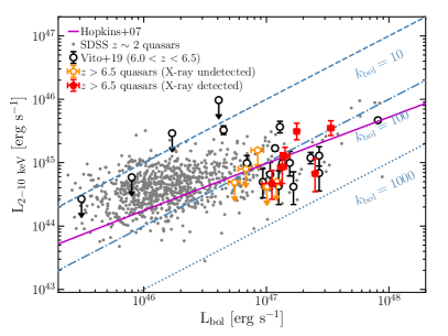
Figure 3: X-ray luminosity, $L_{\rm 2-10keV}$, versus bolometric luminosity, $L_{\rm bol}$, of $z>6.5$ quasars and SDSS $z\sim 2$ quasars. The red pentagons represent X-ray detected $z>6.5$ quasars, while the open orange pentagons denote X-ray undetected $z>6.5$ quasars. The open circles denote quasars at $6.0<z<6.5$ from Vito et al. (2019) and the small grey dots denote SDSS $z\sim 2$ quasars from Timlin et al. (2020). The bolometric correction from $L_{\rm 2-10keV}$ of these $z>6.5$ quasars are $k_{\rm bol}\sim 100$, consistent with the that in lower redshift quasars with similar luminosities (e.g. Hopkins et al., 2007; Martocchia et al., 2017).

Determining the relationship between X-ray luminosity and bolometric luminosity is crucial in estimating the AGN bolometric luminosity function (e.g. Hopkins et al., 2007) and the mass function of SMBH (e.g. Marconi et al., 2004). The relation between $L_{\rm 2-10keV}$ and $L_{\rm bol}$ has been well studied and an increasing bolometric correction $k_{\rm bol}=L_{\rm bol}/L_{\rm 2-10keV}$ with bolometric luminosity has been suggested (e.g. Marconi et al., 2004; Hopkins et al., 2007; Martocchia et al., 2017). In Figure 3, we show the relation between $L_{\rm 2-10keV}$ and $L_{\rm bol}$ of 11 $z>6.5$ quasars, 18 $6<z<6.5$ quasars from Vito et al. (2019) as well as 897 SDSS $z\sim 2$ quasars. The $k_{\rm bol}$ of most SDSS $z\sim 2$ quasars are in the range of $10\lesssim k_{\rm bol}\lesssim 100$, with the most luminous ones at $k_{\rm bol}\sim 100$. The 11 $z>6.5$ quasars have a bolometric luminosity range of $\rm 0.5-3.4\times 10^{47}\,erg\,s^{-1}$ and a X-ray luminosity range of $\rm\lesssim 0.5-3.5\times 10^{45}\,erg\,s^{-1}$, suggesting $k_{\rm bol}\sim 100$. The $k_{\rm bol}$ of these $z>6.5$ quasars is similar to that of the most luminous SDSS $z\sim 2$ quasars and $z\sim 6$ quasars, in agreement with previous studies (e.g. Hopkins et al., 2007; Vito et al., 2019), suggesting a redshift independent relationship between $k_{\rm bol}$ and $L_{\rm bol}$.

4.2 Optical/UV to X-ray Flux Ratio, $\alpha_{\rm ox}$

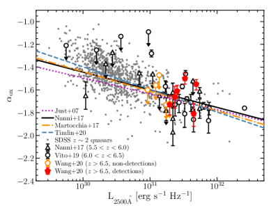
Figure 4: The $\rm\alpha_{ox}$ versus $L_{\rm 2500\AA}$ plot. All symbols have the same meaning as Figure 3, except that we also include quasars at $5.5<z<6.0$ from Nanni et al. (2017) as indicated by open triangles. All data points from literature have been corrected to the cosmology adopted in this work. The $L_{\rm 2500\AA}$ collected from literatures were estimated from the $M_{\rm 1450\AA}$ by assuming a power-law slope of $\alpha_{\nu}=-0.5$, while the $L_{\rm 2500\AA}$ for $z>6.5$ quasars are directly measured from quasar spectra. This plot indicates that there is no redshift evolution of the $\rm\alpha_{ox}-L_{\rm 2500\AA}$ relation.

The $\alpha_{\rm ox}$ measurement traces the relative importance of the disk emission versus corona emission and is an important parameter for investigating the accretion physics of luminous quasars (e.g. Brandt & Alexander, 2015). Previous studies have shown that there is a tight correlation between $\alpha_{\rm ox}$ and $L_{\rm 2500\AA}$ (e.g. Just et al., 2007; Lusso & Risaliti, 2016). Nanni et al. (2017) and Vito et al. (2019) recently used more measurements of high-redshift quasars and showed that the $\alpha_{\rm ox}-L_{\rm 2500\AA}$ relation does not depend on redshift.

We further investigate the $\alpha_{\rm ox}-L_{\rm 2500\AA}$ relationship of high-redshift quasars in three redshift bins with $5.5<z<6.0$ quasars from Nanni et al. (2017), $6.0<z<6.5$ quasars from Vito et al. (2019), and $z>6.5$ quasars from our analysis, which are shown in Figure 4. In this Figure, we also plot $\alpha_{\rm ox}-L_{\rm 2500\AA}$ measured by fitting lower redshift quasars (Just et al., 2007; Martocchia et al., 2017; Timlin et al., 2020) as well as from $z\sim 6$ quasars (Nanni et al., 2017). Our analysis agrees with previous work (e.g. Nanni et al., 2017; Bañados et al., 2018a; Vito et al., 2019) showing a tight $\alpha_{\rm ox}-L_{\rm 2500\AA}$ relation for quasars at different redshifts. In Figure 5, we show the relation between $\rm\Delta\alpha_{ox}$, the difference between the measured $\rm\alpha_{ox}$ and the value expected from the Timlin et al. (2020) $\alpha_{\rm ox}-L_{\rm 2500\AA}$ relation, and quasar redshift. At all redshifts, the $\rm\Delta\alpha_{ox}$ is distributed around zero, indicating that there is no redshift evolution of the $\alpha_{\rm ox}-L_{\rm 2500\AA}$ relationship up to $z\sim 7$. Since $L_{\rm 2500\AA}$ is proportional to $L_{\rm bol}$ (because the $L_{\rm bol}$ was estimated from $L_{\rm 3000\AA}$), and $\alpha_{\rm ox}$ is a relation between $L_{\rm 2500\AA}$ and X-ray luminosity, the lack of redshift evolution of the $\alpha_{\rm ox}-L_{\rm 2500\AA}$ relation is fully consistent with the discussion in §4.1 about the redshift independent relationship between $k_{\rm bol}$ and $L_{\rm bol}$.

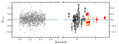
Figure 5: The $\rm\Delta\alpha_{ox}$ versus redshift plot. All symbols have the same meaning as Figure 4.

The Eddington ratio $\lambda_{\rm Edd}$ is the relative accretion rate of the SMBH. Shemmer et al. (2008) and Lusso et al. (2010) found that a weak correlation exists between $\alpha_{\rm ox}$ and $\lambda_{\rm Edd}$ from the analyses of $\sim$30 and $\sim$150 quasars at lower redshifts, respectively. In order to test whether $\alpha_{\rm ox}$ depends on the $\lambda_{\rm Edd}$ at high redshift, we also correlate $\alpha_{\rm ox}$ with $\lambda_{\rm Edd}$ for the 897 SDSS quasars from Timlin et al. (2020) and the $z>6.5$ quasars in Figure 6. Although the relation shows large scatter, a Spearman test gives a correlation coefficient of $\rho=-0.43$ and a chance probability of $p=2.3\times 10^{-41}$, suggesting a moderate $\alpha_{\rm ox}$ - $\lambda_{\rm Edd}$ relation and that the $\alpha_{\rm ox}$ steepens with increasing $\lambda_{\rm Edd}$. Our analysis shows a stronger $\alpha_{\rm ox}$ - $\lambda_{\rm Edd}$ relation compared with that in Shemmer et al. (2008) and Lusso et al. (2010), which could be a natural result of the improved statistics arising from a much larger quasar sample. Nevertheless, the dispersion of this relation is still significant due to the large uncertainty on the individual $\lambda_{\rm Edd}$ measurements, which has a systematic uncertainty up to $\sim 0.55$ dex from the $M_{\rm BH}$ estimate(Vestergaard & Osmer, 2009). On the other hand, we need to keep in mind that $\lambda_{\rm Edd}$ correlates with $L_{\rm 2500\AA}$, thereby the $\alpha_{\rm ox}$ - $\lambda_{\rm Edd}$ relation could also be a consequence of the inherent dependence of $\lambda_{\rm Edd}$ and $L_{\rm 2500\AA}$ as suggested by Shemmer et al. (2008).

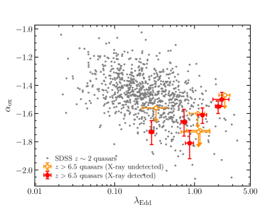
Figure 6: The correlation between $\alpha_{\rm ox}$ and Eddington ratio, $\lambda_{\rm Edd}$. The Spearman test gives $\rho=-0.43$ and $p=2.3\times 10^{-41}$, suggesting a moderate correlation between $\alpha_{\rm ox}$ and $\lambda_{\rm Edd}$. All symbols have the same meaning as Figure 4.

In addition to the broad band SED shape, the relative importance of X-ray and UV emission can also affect the radiation driven wind from the accretion disk, where the X-ray photons can strip the gas of electrons and thereby reduce the line driving, while the UV photons accelerate the wind due to radiation line pressure (the so-called disk+wind model; e.g. Proga et al., 2000; Richards et al., 2011). Therefore, the relatively soft spectrum (smaller $\alpha_{\rm ox}$) would drive a strong wind (e.g. Kruczek et al., 2011). As such, $\alpha_{\rm ox}$ is an important parameter for understanding the radiation driven wind. It is commonly suggested that the blueshift of high-ionization broad emission lines, like C iv, is a marker for radiation driven winds launched from the accretion disk (e.g. Gaskell, 1982; Richards et al., 2011). Thus, one would expect the $\alpha_{\rm ox}$ to be correlated with C iv line blueshift. Indeed, a moderate correlation between $\alpha_{\rm ox}$ and C iv line blueshift have been found at low redshifts (e.g. Richards et al., 2011; Timlin et al., 2020) which supports the paradigm discussed above. On the other hand, recent studies found that the C iv line blueshift of the most distant quasars is about a factor of $\sim$ 2.5 larger than that of lower redshift quasars (e.g. Mazzucchelli et al., 2017; Meyer et al., 2019; Schindler et al., 2020). Investigations of whether the most distant quasars follow the $\alpha_{\rm ox}$ and C iv line blueshift relation found in lower redshift quasars will give us more insights on whether the radiation driven wind in quasars evolves with redshift. In Figure 7, we show the relation between $\alpha_{\rm ox}$ and C iv line blueshift for both $z>6.5$ quasars and SDSS lower redshift quasars. The blueshifts were derived from the redshifts of Mg ii and C iv lines as listed in Table 3. In this Figure, the $z>6.5$ quasars show higher C iv line blueshifts than most of SDSS quasars, but they still follow the blue line derived by Timlin et al. (2020) based solely on SDSS $z\sim 2$ redshift quasars. Although J1342+0928, the most distant quasar in our sample, is far from the relation found by Timlin et al. (2020), such outliers in SDSS quasars with smaller blueshift velocities are also seen in this plot. A larger sample of quasars at $z\sim 7$ with both X-ray and NIR observations are needed to shed more light on this question.

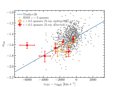
Figure 7: The correlation between $\alpha_{\rm ox}$ and C iv line blueshifts. The Spearman test on all quasars shown in this figure gives $\rho=0.32$ and $p=1.2\times 10^{-23}$, suggesting a moderate relation between these two quantities. All symbols have the same meaning as Figure 4.

4.3 X-ray vs Infrared Luminosity

The observed relations between the masses of SMBHs and the masses of the bulges in their host galaxy suggest a connection between SMBHs and their host galaxies (see Kormendy & Ho, 2013, for a review). The underlying relation between the average host star formation and AGN luminosity found in low redshift high luminosity AGNs (e.g. Alexander et al., 2005; Netzer, 2009; Xu et al., 2015) leads to a relationship between bulge and SMBH growth rates. Recent work by Rosario et al. (2012) finds that the relation between star formation and AGN activity in luminous AGNs weakens or disappears at high redshifts ($z>1$), suggesting an evolutionary relation between SMBH and host galaxy growth rates at high redshifts. In order to investigate whether the quasar X-ray properties (i.e. X-ray luminosity) correlate with quasar host galaxy properties (i.e. $L_{\rm IR}$ or SFR) in the earliest epochs, we plot the $L_{\rm IR}$ and $L_{\rm 2-10keV}$ of all objects as described in § 3 in Figure 8. From Figure 8, there is no correlation ($\rho=-0.19$, p=0.10) between $L_{\rm IR}$ (or SFR) and $L_{\rm 2-10keV}$ for both SDSS $z\sim 2$ quasars and high-$z$ quasars, different from that in lower redshift ($z<1$) AGNs (e.g. Netzer, 2009; Xu et al., 2015). The lack of a correlation between $L_{\rm IR}$ and $L_{\rm 2-10keV}$ of these luminous quasars is also consistent with the absence of a correlation between $L_{\rm IR}$ and $L_{\rm bol}$ of $z\gtrsim 6$ quasars (Venemans et al., 2018) and the high mass ratio between SMBHs and their host galaxies (e.g. Decarli et al., 2018; Wang et al., 2019a), indicating that SMBHs of the most luminous quasars in the early epochs do not co-evolve with their host galaxies, at least not following the same relation found in low redshift galaxies (e.g. Alexander et al., 2005; Netzer, 2009; Kormendy & Ho, 2013). We emphasize that our quasar sample only represents the UV brightest quasar population at high redshift and the conclusion can only apply to these most luminous objects.

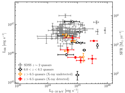
Figure 8: Infrared luminosity, $L_{\rm IR}$, versus X-ray luminosity, $L_{\rm 2-10keV}$. The Spearman test gives $\rho=-0.19$ and p=0.10, suggesting no correlation between the star formation rate (as indicated by $L_{\rm IR}$) and AGN activity (as indicated by $L_{\rm 2-10keV}$), different from that found in low redshift AGNs (e.g. Alexander et al., 2005; Netzer, 2009; Xu et al., 2015). All symbols have the same meaning as Figure 4.

Moreover, Figure 8 shows that the $L_{\rm IR}$ of the most luminous (e.g. $L_{\rm 2-10keV}\gtrsim 10^{45}~{}{\rm erg~{}s^{-1}}$) $z>6.5$ quasars is even fainter than that of X-ray fainter ones (e.g. $L_{\rm 2-10keV}<10^{45}~{}{\rm erg~{}s^{-1}}$) and most SDSS quasars. However, as we mentioned in § 3, the Herschel detected SDSS quasars only represent the $\sim$15% infrared bright quasars limited by the depth of Herschel observations, thus some of the Herschel undetected SDSS quasars could have similar infrared-to-X-ray luminosity ratios with $z>6.5$ quasars. Nevertheless, there is no $z>6.5$ quasar having $L_{\rm IR}$ close to $\rm 10^{47}erg~{}s^{-1}$ and several X-ray bright high-$z$ quasars with $L_{\rm IR}<10^{46}{\rm erg~{}s^{-1}}$ suggests that these powerful AGN with strong disk driven wind, as indicated by the high Eddington ratio (Figure 6) and large C iv blueshift (Figure 7), could suppress star formation activities in their host galaxies. However, our current sample is too small to obtain definitive conclusions and a systematic survey of the X-ray and far-infrared properties of a larger $z>6.5$ quasar sample would be critical to test this scenario.

5 Average X-ray Properties of $z\sim 7$ Quasars

Measuring the X-ray spectral properties for individual quasars requires a significant number of detected X-ray counts. In this work, we do not attempt to fit the individual quasar X-ray spectrum due to the limitation of small number of photons detected. Instead, we measure the average hard X-ray photon index of these $z>6.5$ quasars using two different methods. First, we perform a joint spectral analysis of the six $z>6.5$ quasars that are well detected in the X-ray (see Table 2). The average redshift of these six quasars is $z=6.822$ and the total net counts in the 0.5–7 keV band is $\sim$64. We jointly fit these quasar spectra with a power-law model and associate a value of redshift and Galactic absorption to each source using XSPEC. From the joint fit, we derive a photon index $\Gamma=2.32^{+0.31}_{-0.30}$. We use the Cash statistic and report the uncertainties at the 68% confidence level. As a further test, we stack the spectra of these six detected $z>6.5$ quasars. The stacked spectrum is shown in Figure 9. We use XSPEC to fit this stacked spectrum with a power-law by fixing the Galactic absorption component to the mean $N_{\rm H}$ and the redshift to $z=6.822$. The derived photon index from the stacked spectrum fitting is $\Gamma=2.11^{+0.27}_{-0.26}$, consistent with the photon index obtained by the joint spectral fitting.

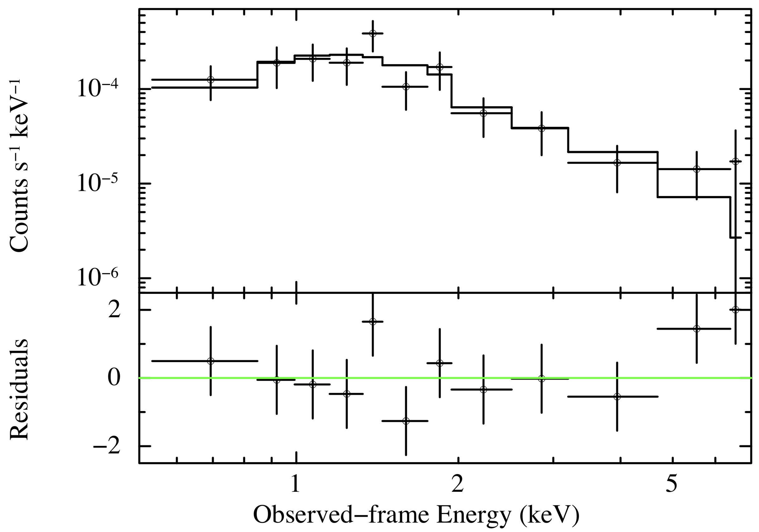
Figure 9: Stacked X-ray spectrum of six X-ray detected $z>6.5$ quasars. The mean redshift of these quasars is $z=6.822$. The black solid line is the best-fit power-law model with a photon index of $\Gamma=2.11^{+0.27}_{-0.26}$, consistent with $\Gamma=2.32^{+0.31}_{-0.30}$, derived from the joint spectral fitting. The bottom panel shows the residuals (data$-$model).

Vito et al. (2019) jointly analyzed three $z>6.5$ quasars ($\sim$23 net counts in total) and found $\Gamma=2.66^{+0.54}_{-0.50}$. The average $\Gamma$ measured by Vito et al. (2019) is slightly steeper than (although with large uncertainties) the average $\Gamma$ found at lower redshifts, which is $\Gamma\sim 1.9$ (Piconcelli et al., 2005; Vignali et al., 2005; Shemmer et al., 2006; Just et al., 2007; Nanni et al., 2017). In the left panel of Figure 10, we show the average $\Gamma$ measured from joint spectral fitting of quasars at different cosmic epochs. Our newly measured $\Gamma$ is slightly steeper than that for lower redshift quasars, consistent with the value measured by Vito et al. (2019) but with smaller uncertainties.

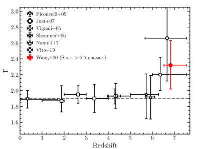
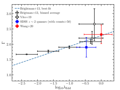
Figure 10: Left: Photon index, $\Gamma$, as a function of redshift. Our joint spectra fitting result ($\Gamma=2.32^{+0.31}_{-0.30}$) at $z=6.822$ is highlighted with a red pentagon. The gray dashed line denotes $\rm\Gamma=1.9$. In all cases, the assumed model is a power-law and errors are reported at the 68% confidence level. Right: Photon index, $\Gamma$, as a function of Eddington ratio, $\lambda_{\rm Edd}$. Our new measurement based on the joint fitting of six X-ray detected $z>6.5$ quasars is highlighted as a red pentagon. The two measurements by Vito et al. (2019) are shown as big open circles. The small open circles denote binned averages measurements of a sample of $z\lesssim 2$ quasars with both X-ray observations and BH mass estimates and the dashed line represents the best-fit model (Brightman et al., 2013).

Since the $\Gamma$ value of a quasar’s hard X-ray spectrum correlates with the $\lambda_{\rm Edd}$ value as suggested by numerous works (e.g. Porquet et al., 2004; Shemmer et al., 2008; Brightman et al., 2013), it is necessary to check whether the steeper hard X-ray spectral slope at $z>6.5$ is due to quasars with high Eddington ratios. Since not all quasars studied in these joint spectral analyses (e.g. Porquet et al., 2004; Shemmer et al., 2008; Brightman et al., 2013) have Eddington ratio measurements, we can not compare the Eddington ratios of these quasars used for joint spectral analyses directly. Instead, we compare the average $\Gamma$ and $\lambda_{\rm Edd}$ of our $z>6.5$ quasars with the relation found by Brightman et al. (2013) from a well studied AGN sample at $0.5\lesssim z\lesssim 2.0$ in the Cosmic Evolution Survey (COSMOS) and Extended Chandra Deep Field South (E-CDF-S) field. In the right panel of Figure 10 we show the measurements and relation from Brightman et al. (2013) as well as our measurement at $z>6.5$. In this Figure, we also show the average $\Gamma$ and $\lambda_{\rm Edd}$ of the $z\gtrsim 6$ quasars from Vito et al. (2019) and SDSS $z\sim 2$ quasars. Note that the average $\Gamma$ of $z\sim 2$ SDSS quasars is directly measured from the X-ray spectral fitting by Timlin et al. (2020) and only includes $\sim 100$ quasars with $>50$ net counts selected from our $z\sim 2$ comparison quasar sample (see §4). This plot indicates that the steeper hard X-ray slope of the $z>6.5$ quasars from our analysis and the previous study by Vito et al. (2019) are fully consistent with the $\Gamma$ and $\lambda_{\rm Edd}$ relation found in lower-$z$ quasars, suggesting that the steeper $\Gamma$ of $z>6.5$ quasars is mainly driven by their higher Eddington ratios rather than by their higher redshifts.

6 Summary

In this paper, we present new Chandra observations of five quasars at $z>6.5$. By combining them with archival Chandra observations of an additional six $z>6.5$ quasars, we perform a systematic analysis of the X-ray properties of these reionization-era quasars. Six of these eleven $z>6.5$ quasars are well detected with a luminosity range of $L_{\rm 2-10keV}\sim(4.7-35.3)\times 10^{44}~{}{\rm erg~{}s^{-1}}$. In addition, we analyze the infrared spectroscopic observations of these Chandra observed $z>6.5$ quasars and derive the bolometric luminosities, BH masses, Eddington ratios, and broad emission line blueshifts for all quasars. The bolometric luminosities of these sources span a range of $L_{\rm bol}\sim(0.5-3.4)\times 10^{47}~{}{\rm erg~{}s^{-1}}$, occupying the bright end of the quasar population. Their masses and Eddington ratios are in the range $(0.2-3.0)\times 10^{9}~{}M_{\odot}$ and $\sim 0.3-2.4$, respectively. We also measure the infrared luminosity ($L_{\rm IR}$) and star formation rate (SFR) of the quasar host galaxies yielding $L_{\rm IR}$ in the range of $(0.5-4.5)\rm\times 10^{46}~{}erg~{}s^{-1}$ and SFR in the range of $\sim 200-2000~{}M_{\odot}~{}{\rm yr^{-1}}$, respectively. Moreover, we perform a joint spectral analyses of all X-ray detected quasars and measure the average X-ray spectral properties of these $z>6.5$ quasars. Our findings from this unique sample of $z>6.5$ quasar with both X-ray and near-infrared spectroscopic observations, and based on a comparison quasar sample at $z\sim 2$, are as follows:

• The X-ray bolometric luminosity correction ($k_{\rm bol}=L_{\rm bol}/L_{\rm 2-10keV}$) of $z>6.5$ quasars increases with bolometric luminosity and the optical/UV to X-ray flux ratio, $\alpha_{\rm ox}$, strongly correlates with quasar luminosity at rest-frame 2500 Å, $L_{\rm 2500\AA}$, following the same trend found in lower redshift quasars.

• A moderate correlation between $\alpha_{\rm ox}$ and Eddington ratio, $\lambda_{\rm Edd}$, exists. This correlation is weaker than the $\alpha_{\rm ox}$-$L_{\rm 2500\AA}$ relation, which could either be a consequence of the inherent dependence of $\lambda_{\rm Edd}$ and $L_{\rm 2500\AA}$ or result from the large uncertainty introduced by the $\lambda_{\rm Edd}$ measurement.

• The $L_{\rm IR}$ and SFR do not correlate with the $L_{\rm 2-10keV}$ in these luminous distant quasars, suggesting that the ratio of the SMBH growth rate and their host galaxy growth rate in these early luminous quasars are different from that of local galaxies.

• There is a moderate correlation between $\alpha_{\rm ox}$ and C iv line blueshift. In the disc+wind model picture (e.g. Gaskell, 1982; Richards et al., 2011), the C iv line blueshift increases as the relative importance of corona X-ray emission and accretion disk emission decreases, consistent with the observed correlation.

• The average photon index, $\Gamma$, of hard X-ray spectra of $z>6.5$ quasars is found to be $\Gamma=2.32^{+0.31}_{-0.30}$, steeper than that of lower redshift quasars. By comparing our measurement with the $\Gamma$-$\lambda_{\rm Edd}$ relation found in lower redshift quasars (e.g. Brightman et al., 2013), we conclude that the steeper $\Gamma$ of $z>6.5$ quasars is mainly driven by their higher Eddington ratios rather than by their higher redshifts.

In the near future, a larger sample of $z>6.5$ quasars with both X-ray, NIR, and sub-millimeter observations, as well as a well matched (in terms of both quasar luminosity and observational depth) quasar sample at lower redshifts is critical for investigating whether the earliest SMBHs are fed by different accretion physics (especially the X-ray luminosity and $\Gamma$) and arise in distinct galactic environments (i.e. star formation rate) relative to their lower redshift counterparts.

References

- Ai et al. (2016) Ai, Y., Dou, L., Fan, X., et al. 2016, ApJ, 823, L37
- Ai et al. (2017) Ai, Y., Fabian, A. C., Fan, X., et al. 2017, MNRAS, 470, 1587
- Alexander et al. (2005) Alexander, D. M., Bauer, F. E., Chapman, S. C., et al. 2005, ApJ, 632, 736
- Antonucci (1993) Antonucci, R. 1993, ARA&A, 31, 473
- Arnaud et al. (1985) Arnaud, K. A., Branduardi-Raymont, G., Culhane, J. L., et al. 1985, MNRAS, 217, 105
- Arnaud (1996) Arnaud, K. A. 1996, Astronomical Data Analysis Software and Systems V, 101, 17
- Bañados et al. (2018b) Bañados, E., Connor, T., Stern, D., et al. 2018b, ApJ, 856, L25
- Bañados et al. (2015) Bañados, E., Decarli, R., Walter, F., et al. 2015, ApJ, 805, L8
- Bañados et al. (2016) Bañados, E., Venemans, B. P., Decarli, R., et al. 2016, ApJS, 227, 11
- Bañados et al. (2018a) Bañados, E., Venemans, B. P., Mazzucchelli, C., et al. 2018a, Nature, 553, 473
- Beelen et al. (2006) Beelen, A., Cox, P., Benford, D. J., et al. 2006, ApJ, 642, 694
- Betoule et al. (2014) Betoule, M., Kessler, R., Guy, J., et al. 2014, A&A, 568, A22
- Bochanski et al. (2009) Bochanski, J. J., Hennawi, J. F., Simcoe, R. A., et al. 2009, PASP, 121, 1409
- Brandt & Alexander (2015) Brandt, W. N., & Alexander, D. M. 2015, A&A Rev., 23, 1
- Brandt et al. (2001) Brandt, W. N., Guainazzi, M., Kaspi, S., et al. 2001, AJ, 121, 591
- Brightman et al. (2013) Brightman, M., Silverman, J. D., Mainieri, V., et al. 2013, MNRAS, 433, 2485
- Cardelli et al. (1989) Cardelli, J. A., Clayton, G. C., & Mathis, J. S. 1989, ApJ, 345, 245
- Clough et al. (2005) Clough, S. A., Shephard, M. W., Mlawer, E. J., et al. 2005, J. Quant. Spec. Radiat. Transf., 91, 233
- Connor et al. (2020) Connor, T., Bañados, E., Mazzucchelli, C., et al. 2020, ApJ, in press
- Connor et al. (2019) Connor, T., Bañados, E., Stern, D., et al. 2019, ApJ, 887, 171
- Davies et al. (2018) Davies, F. B., Hennawi, J. F., Bañados, E., et al. 2018, ApJ, 864, 143
- Decarli et al. (2018) Decarli, R., Walter, F., Venemans, B. P., et al. 2018, ApJ, 854, 97
- De Rosa et al. (2014) De Rosa, G., Venemans, B. P., Decarli, R., et al. 2014, ApJ, 790, 145
- Elias et al. (2006a) Elias, J. H., Rodgers, B., Joyce, R. R., et al. 2006, Proc. SPIE, 626914
- Elias et al. (2006b) Elias, J. H., Joyce, R. R., Liang, M., et al. 2006, Proc. SPIE, 62694C
- Fabian et al. (2014) Fabian, A. C., Walker, S. A., Celotti, A., et al. 2014, MNRAS, 442, L81
- Fan et al. (2001) Fan, X., Narayanan, V. K., Lupton, R. H., et al. 2001, AJ, 122, 2833
- Freeman et al. (2001) Freeman, P., Doe, S., & Siemiginowska, A. 2001, Proc. SPIE, 4477, 76
- Freeman et al. (2002) Freeman, P. E., Kashyap, V., Rosner, R., & Lamb, D. Q. 2002, ApJS, 138, 185
- Fruscione et al. (2006) Fruscione, A., McDowell, J. C., Allen, G. E., et al. 2006, Proc. SPIE, 6270, 62701V
- Garmire et al. (2003) Garmire, G. P., Bautz, M. W., Ford, P. G., Nousek, J. A., & Ricker, G. R., Jr. 2003, Proc. SPIE, 4851, 28
- Gaskell (1982) Gaskell, C. M. 1982, ApJ, 263, 79
- Gehrels (1986) Gehrels, N. 1986, ApJ, 303, 336
- Germain et al. (2006) Germain, G., Milaszewski, R., McLaughlin, W., et al. 2006, Astronomical Data Analysis Software and Systems XV, 351, 57
- Hopkins et al. (2007) Hopkins, P. F., Richards, G. T., & Hernquist, L. 2007, ApJ, 654, 731
- Horne (1986) Horne, K. 1986, PASP, 98, 609
- Inayoshi et al. (2019) Inayoshi, K., Visbal, E., & Haiman, Z. 2019, arXiv e-prints, arXiv:1911.05791
- Jiang et al. (2016) Jiang, L., McGreer, I. D., Fan, X., et al. 2016, ApJ, 833, 222
- Just et al. (2007) Just, D. W., Brandt, W. N., Shemmer, O., et al. 2007, ApJ, 665, 1004
- Kalberla et al. (2005) Kalberla, P. M. W., Burton, W. B., Hartmann, D., et al. 2005, A&A, 440, 775
- Kormendy & Ho (2013) Kormendy, J., & Ho, L. C. 2013, ARA&A, 51, 511
- Kruczek et al. (2011) Kruczek, N. E., Richards, G. T., Gallagher, S. C., et al. 2011, AJ, 142, 130
- Latif & Ferrara (2016) Latif, M. A., & Ferrara, A. 2016, PASA, 33, e051
- Lusso et al. (2010) Lusso, E., Comastri, A., Vignali, C., et al. 2010, A&A, 512, A34
- Lusso & Risaliti (2016) Lusso, E., & Risaliti, G. 2016, ApJ, 819, 154
- Lyu et al. (2016) Lyu, J., Rieke, G. H., & Alberts, S. 2016, ApJ, 816, 85
- Maraschi & Haardt (1997) Maraschi, L., & Haardt, F. 1997, IAU Colloq. 163: Accretion Phenomena and Related Outflows, 121, 101
- Marconi et al. (2004) Marconi, A., Risaliti, G., Gilli, R., et al. 2004, MNRAS, 351, 169
- Martocchia et al. (2017) Martocchia, S., Piconcelli, E., Zappacosta, L., et al. 2017, A&A, 608, A51
- Matsuoka et al. (2019) Matsuoka, Y., Onoue, M., Kashikawa, N., et al. 2019, ApJ, 872, L2
- Mazzucchelli et al. (2017) Mazzucchelli, C., Bañados, E., Venemans, B. P., et al. 2017, ApJ, 849, 91
- Meyer et al. (2019) Meyer, R. A., Bosman, S. E. I., & Ellis, R. S. 2019, MNRAS, 487, 3305
- Moretti et al. (2014) Moretti, A., Ballo, L., Braito, V., et al. 2014, A&A, 563, A46
- Mortlock et al. (2011) Mortlock, D. J., Warren, S. J., Venemans, B. P., et al. 2011, Nature, 474, 616
- Nanni et al. (2018) Nanni, R., Gilli, R., Vignali, C., et al. 2018, A&A, 614, A121
- Nanni et al. (2017) Nanni, R., Vignali, C., Gilli, R., Moretti, A., & Brandt, W. N. 2017, A&A, 603, A128
- Netzer (2009) Netzer, H. 2009, MNRAS, 399, 1907
- Omukai et al. (2008) Omukai, K., Schneider, R., & Haiman, Z. 2008, ApJ, 686, 801
- Onoue et al. (2020) Onoue, M., Bañados, E., Mazzucchelli, C., et al. 2020, arXiv:2006.16268
- Page et al. (2014) Page, M. J., Simpson, C., Mortlock, D. J., et al. 2014, MNRAS, 440, L91
- Park et al. (2006) Park, T., Kashyap, V. L., Siemiginowska, A., et al. 2006, ApJ, 652, 610
- Parker et al. (2017) Parker, M. L., Pinto, C., Fabian, A. C., et al. 2017, Nature, 543, 83
- Piconcelli et al. (2005) Piconcelli, E., Jimenez-Bailón, E., Guainazzi, M., et al. 2005, A&A, 432, 15
- Pons et al. (2020) Pons, E., McMahon, R. G., Banerji, M., et al. 2020, MNRAS, 491, 3884
- Porquet et al. (2004) Porquet, D., Reeves, J. N., O’Brien, P., et al. 2004, A&A, 422, 85
- Prochaska et al. (2020a) Prochaska, J. X., Hennawi, J., Cooke, R., et al. 2020, pypeit/PypeIt: Release 1.0.0, v1.0.0, Zenodo, doi:10.5281/zenodo.3506872
- Prochaska et al. (2020b) Prochaska, J. X., Hennawi, J. F., Westfall, K. B., et al. 2020, arXiv e-prints, arXiv:2005.06505
- Proga et al. (2000) Proga, D., Stone, J. M., & Kallman, T. R. 2000, ApJ, 543, 686
- Richards et al. (2011) Richards, G. T., Kruczek, N. E., Gallagher, S. C., et al. 2011, AJ, 141, 167
- Reed et al. (2017) Reed, S. L., McMahon, R. G., Martini, P., et al. 2017, MNRAS, 468, 4702
- Rosario et al. (2012) Rosario, D. J., Santini, P., Lutz, D., et al. 2012, A&A, 545, A45
- Schindler et al. (2020) Schindler, J. T., Farina, E. P., Walter, F., et al. 2020, ApJ, submitted
- Schlegel et al. (1998) Schlegel, D. J., Finkbeiner, D. P., & Davis, M. 1998, ApJ, 500, 525
- Shemmer et al. (2008) Shemmer, O., Brandt, W. N., Netzer, H., Maiolino, R., & Kaspi, S. 2008, ApJ, 682, 81
- Shemmer et al. (2006) Shemmer, O., Brandt, W. N., Schneider, D. P., et al. 2006, ApJ, 644, 86
- Shen et al. (2011) Shen, Y., Richards, G. T., Strauss, M. A., et al. 2011, ApJS, 194, 45
- Shields (1978) Shields, G. A. 1978, Nature, 272, 706
- Simcoe et al. (2010) Simcoe, R. A., Burgasser, A. J., Bochanski, J. J., et al. 2010, Proc. SPIE, 773514
- Svensson & Zdziarski (1994) Svensson, R., & Zdziarski, A. A. 1994, ApJ, 436, 599
- Tang et al. (2017) Tang, J.-J., Goto, T., Ohyama, Y., et al. 2017, MNRAS, 466, 4568
- Tang et al. (2019) Tang, J.-J., Goto, T., Ohyama, Y., et al. 2019, MNRAS, 484, 2575
- Tegmark et al. (1997) Tegmark, M., Silk, J., Rees, M. J., et al. 1997, ApJ, 474, 1
- Timlin et al. (2020) Timlin, J. D., Brandt, W. N., Ni, Q., et al. 2020, MNRAS, 492, 719
- Trakhtenbrot et al. (2017) Trakhtenbrot, B., Ricci, C., Koss, M. J., et al. 2017, MNRAS, 470, 800
- Tsuzuki et al. (2006) Tsuzuki, Y., Kawara, K., Yoshii, Y., et al. 2006, ApJ, 650, 57
- Venemans et al. (2018) Venemans, B. P., Decarli, R., Walter, F., et al. 2018, ApJ, 866, 159
- Venemans et al. (2013) Venemans, B. P., Findlay, J. R., Sutherland, W. J., et al. 2013, ApJ, 779, 24
- Venemans et al. (2016) Venemans, B. P., Walter, F., Zschaechner, L., et al. 2016, ApJ, 816, 37
- Vernet et al. (2011) Vernet, J., Dekker, H., D’Odorico, S., et al. 2011, A&A, 536, A105
- Vestergaard & Osmer (2009) Vestergaard, M., & Osmer, P. S. 2009, ApJ, 699, 800
- Vestergaard & Wilkes (2001) Vestergaard, M., & Wilkes, B. J. 2001, ApJS, 134, 1
- Vignali et al. (2005) Vignali, C., Brandt, W. N., Schneider, D. P., et al. 2005, AJ, 129, 2519
- Vito et al. (2019) Vito, F., Brandt, W. N., Bauer, F. E., et al. 2019, A&A, 630, A118
- Volonteri et al. (2008) Volonteri, M., Lodato, G., & Natarajan, P. 2008, MNRAS, 383, 1079
- Volonteri et al. (2015) Volonteri, M., Silk, J., & Dubus, G. 2015, ApJ, 804, 148
- Wang et al. (2017) Wang, F., Fan, X., Yang, J., et al. 2017, ApJ, 839, 27
- Wang et al. (2018) Wang, F., Yang, J., Fan, X., et al. 2018, ApJ, 869, L9
- Wang et al. (2019a) Wang, F., Wang, R., Fan, X., et al. 2019a, ApJ, 880, 2
- Wang et al. (2019b) Wang, F., Yang, J., Fan, X., et al. 2019b, ApJ, 884, 30
- Wang et al. (2020) Wang, F., Davies, F. B., Yang, J., et al. 2020, ApJ, 896, 23
- Wise et al. (2019) Wise, J. H., Regan, J. A., O’Shea, B. W., et al. 2019, Nature, 566, 85
- Wu et al. (2015) Wu, X.-B., Wang, F., Fan, X., et al. 2015, Nature, 518, 512
- Xu et al. (2015) Xu, L., Rieke, G. H., Egami, E., et al. 2015, ApJ, 808, 159
- Yang et al. (2017) Yang, J., Fan, X., Wu, X.-B., et al. 2017, AJ, 153, 184
- Yang et al. (2019) Yang, J., Wang, F., Fan, X., et al. 2019, AJ, 157, 236
- Yang et al. (2020) Yang, J., Wang, F., Fan, X., et al. 2020, ApJ, 897, L14