Extremely rare ultra-fast non-equilibrium processes can be close to equilibrium: RNA unfolding and refolding

Abstract

We study numerically the behavior of RNA secondary structures under influence of a varying external force. This allows to measure the work $W$ during the resulting fast unfolding and refolding processes. Here, we investigate a medium-size hairpin structure. Using a sophisticated large-deviation algorithm, we are able to measure work distributions with high precision down to probabilities as small as $10^{-46}$. Due to this precision and by comparison with exact free-energy calculations we are able to verify the theorems of Crooks and Jarzynski. Furthermore, we analyze force-extension curves and the configurations of the secondary structures during unfolding and refolding for typical equilibrium processes and non-equilibrium processes, conditioned to selected values of the measured work $W$, typical and rare ones. We find that the non-equilibrium processes where the work values are close to those which are most relevant for applying Crooks and Jarzynski theorems, respectively, are most and quite similar to the equilibrium processes. Thus, a similarity of equilibrium and non-equilibrium behavior with respect to a mere scalar variable, which occurs with a very small probability but can be generated in a controlled but non-targeted way, is related to a high similarity for the set of configurations sampled along the full dynamical trajectory.

In Statistical Physics, the cleanest and so far best-justified description is obtained for systems in equilibrium. Nevertheless, due to open system boundaries and lack of infinite time to perform experiments or simulations, most real and simulated model systems are constantly in non-equilibrium. A bridge between both worlds is provided. e.g., by the theorems of Jarzynski Jarzynski (1997a) and Crooks Crooks (1998), where the distribution $P(W)$ of work $W$ is measured for arbitrary fast non-equilibrium processes obtained from sampling equilibrium initial configurations and possibly stochastic non-equilibrium trajectories. Correspondingly $P_{\rm rev}(W)$ is the distribution for the reverse process. For a system coupled to a heat bath, Crooks theorem reads $P(W)=P_{\rm rev}(-W)\exp(-(\Delta F-W)/T)$. This can be used to reconstruct the true free energy difference $\Delta F$ between initial and final state, because $P(W)$ and $P_{\rm rev}(-W)$ cross at $W=\Delta F$. Correspondingly the equation of Jarzynski reads $\langle e^{-W/T}\rangle=e^{-\Delta F/T}$. These and related theorems have lead to many applications and extensions relating equilibrium and non-equilibrium processes Kurchan (2007); Seifert (2008); Sevick et al. (2008); Jarzynski (2008); Esposito et al. (2009); Jarzynski (2011); Seifert (2012); Marsland III and England (2018). A fruitful field of applications is biophysics, where these theorems are used to measure properties of small molecules like RNA.

One major goal of stochastic thermodynamics is to extract equilibrium information from non-equilibrium measurements or simulations Hartmann (2015). The fluctuation theorems concern specific measurable scalar quantities like work Jarzynski (1997a); Crooks (1998); Hummer and Szabo (2010), entropy Evans et al. (1993); Evans and Searles (1994); Gallavotti and Cohen (1995a, b); Kurchan (1998); Lebowitz and Spohn (1999); Maes (1999); Crooks (1999, 2000), or a quantity measuring the volume of the phase space Adib (2005). However, beyond statistics of particular scalar quantities, the fluctuation theorems do not provide information about the unseen equilibrium behavior along the trajectory, i.e., with respect to arbitrary measurable quantities. Standard derivations of the fluctuations theorems only involve terms which include energies and probabilities of the initial and final state. What may we expect when we analyze the full trajectory of a non-equilibrium process? First, a typical, i.e., highly probable sample of a non-equilibrium trajectory will look very different from a corresponding trajectory sampled during an equilibrium process. Second, it is known that when reweighting trajectories suitably in a time-dependent way, they also carry some information about the intermediate not-seen equilibrium states Jarzynski (1997b); Crooks (2000); Hummer and Szabo (2001) which allows for the reconstruction of full free-energy profiles beyond initial and final state. Third, it is somehow intuitive to believe that the rare non-equilibrium processes which contribute most to the estimation of $\Delta F$ are in a comprehensive way, without reweighting, similar or even equal to the corresponding equilibrium processes. For the case of the theorems of Crooks and Jarzynski, the statistics of the work distributions are most relevant for particular work values $W=\Delta F$ and $W=W_{\rm J}^{*}$, where the latter one is the value where the integrand $e^{-W/T}P(W)$ exhibits a maximum. Note that these values are high improbable to occur for large system sizes. On the other hand, beyond this intuition, there is no solid reason that these rare possibly very fast processes completely resemble true equilibrium processes: A non-equilibrium process always depends on the history, i.e., on many configurations encountered so far, while each equilibrium state in a process does not depend at all on the history. In particular, non-equilibrium processes depend on the speed of performance, while the equilibrium is for infinite low speed.

This question motivates our present work: We investigate in a comprehensive way the dynamics of fast non-equilibrium processes conditioned to various non-equilibrium work values $W$, typical and rare ones, and compare with the equilibrium process behavior. In particular, we study unfolding and refolding of RNA secondary structures subject to an external force Müller et al. (2002). The former one, denoted as forward process, involves stretching an RNA by subjecting it to an external force $f$ which is increased from starting at zero. For the latter one, denoted as reverse process, one starts with a large force and reduces it to zero. For small RNAs consisting of few dozens of bases, Crooks theorem has been confirmed in experiments and simulations Hummer and Szabo (2010) for slow unfolding and refolding processes. For such small RNA and slow processes, the resulting work distributions are rather broad and the distribution for forward and reverse processes are close to each other such that they cross at high-probability values which are easily accessible. For larger RNA molecules, the crossing points will move to smaller probabilities, such that the crossing cannot be observed in experiments or standard simulations. To go beyond such limiting system sizes, we applied for our study sophisticated large-deviation algorithms Hartmann (2002); Bucklew (2004), which allowed us to measure probability distributions numerically down to extremely small probabilities. These algorithms have also applied successfully to non-equilibrium processes like the transition-path sampling approach to study protein folding Dellago et al. (1998); Bolhuis et al. (2002), population-based approaches to study asymmetric exclusion processes Giardinà et al. (2006); Lecomte and Tailleur (2007) or Markov-chain Monte Carlo methods to investigate, e.g., traffic models Staffeldt and Hartmann (2019) and the Kardar-Parisi-Zhang equation Hartmann et al. (2018). In particular such an algorithm has also been applied to measure with high precision the work distribution of an Ising model subject to a varying external field Hartmann (2014), providing the first confirmation of the theorems of Jarzynski and Crooks for a large system with many thousands of particles.

Thus, here we will provide similar evidence for RNA secondary structure unfolding and refolding by applying such a rare-event algorithm, allowing us to obtain the work distributions of intermediate-sized RNAs down to probabilities as small as $10^{-46}$. Furthermore, we will analyze the temporal structure of the non-equilibrium processes, conditioned to the occurring work values $W$. We will compare this to the corresponding equilibrium process, which can be sampled exactly Higgs (1996); Burghardt and Hartmann (2005); Lorenz et al. (2011) and efficiently, i.e., in polynomial time, for RNA secondary structures without pseudo-knots. Beyond confirming the theorems of Jarzynski and Crooks we find in particular that the non-equilibrium processes can be very similar in their development to the equilibrium ones. The highest similarity is reached for processes which exhibit a work value $W$ between the values $W=\Delta F$ and $W=W_{\rm J}^{*}$ which are most relevant for the Crooks and Jarzynski theorem, respectively.

We will next present our model and the simulation methods we used. Then we show our results and finish by a discussion.

Model — Each RNA molecule is a linear chain of length $L$ of bases from $\{\mathrm{A,C,G,U}\}$. A secondary structure is a set of pairs of bases, such that only complementary (Watson-Crick) base pairs A-U and C-G are allowed. We forbid pseudo-knots, which means that it is always possible to draw the molecule as a single line and connect all pairs by lines such that no intersections occur.

The energy of an RNA secondary structure consists, first, of the energy from the Watson-Crick pairs, which is its number here for simplicity. Second, the RNA is subject to a force $f$. This gives rise to an energy contribution $-f\times n$ where $n$ is the extension of the structure, i.e., the part of the RNA which is outside any paired base, plus length 2 for any paired base on the first level. For details see the supplementary material (SM).

Algorithms — For RNA secondary structures it is possible to sample them directly in equilibrium for finite temperatures $T$ in time $O(L^{3})$. We used an extension of the approach for the zero-force case Higgs (1996). For this purpose, one needs also to calculate partitions functions for some sub sequences, which is possible using dynamic programming in polynomial time. These approaches Gerland et al. (2001); Müller et al. (2002) are also extensions of the zero-force case approach Nussinov et al. (1978). For details see the SM.

For actually performing an unfolding or refolding process, and to measure the performed work $W$, we started with a configuration $\mathcal{S}_{0}$ sampled in equilibrium at initial force $f=f_{0}$ with $f_{0}=0$ or $f_{0}=f_{\max}=2$. Then the force $f$ was gradually changed in steps $\Delta f$ up to $f_{\max}$ or down to zero, respectively, while allowing for thermal fluctuations by performing Monte Carlo simulations with creation or removal of pairs as basic moves. Each time the force is changed, we obtained a contribution $\Delta W=-n(\mathcal{S})\Delta f$ to the work, where $n(\mathcal{S})$ is the current extension. For details of the algorithm see the SM.

By repeating an unfolding or refolding simulation many times, one can measure approximately the work distributions $P(W)$ and $P_{\rm rev}(W)$, respectively. Nevertheless, this simple sampling approach allows one only to obtain the work distributions down to rather large probabilities, like $10^{-9}$. To obtain the work distributions down to much smaller probabilities, we applied sophisticated large-deviation algorithms Hartmann (2002); Bucklew (2004). Our approach has already been used to measure work distributions for large Ising systems Hartmann (2014). The basic idea is to drive the forward and reverse processes, respectively, by vectors $\xi$ of random numbers and control the composition of the vectors with a Markov chain Monte Carlo simulation, with a known, i.e., removable, bias depending on the measured work. For details see the SM.

Results — We considered an RNA sequence which is not too small, such that we were able to observe differences between equilibrium and non-equilibrium secondary structure configurations with suitable resolution. We studied a hairpin structure of length $L=100$ which has a sequence (AC)²⁵(UG)²⁵, resulting in a ground state of one large stack with a small hairpin. For such an RNA size the application of large-deviation algorithm is necessary to measure the work distribution with suitable accuracy such that the theorems of Jarzynski and Crooks can be applied and the unfolding and refolding histories captured. We considered the RNA coupled to a heat bath at temperatures $T=0.3$ and $T=1$, respectively. These are low enough temperatures, such that in the force-free case, the RNA is basically folded, but exhibits thermal fluctuations. Example secondary structures are shown in a figure in the SM. We considered two different speeds of the folding processes, i.e., two different numbers $n_{\rm MC}$ of sweeps performed during the process, here $n_{\rm MC}=8$ and $n_{\rm MC}=16$. A summary of the simulation parameters is also given in the SM.

Figure 1: Plain and mirrored work distributions for $T=1$ and 8 sweeps of the forward and reverse process, respectively. They intersect near $W=\Delta F$, which is the exact value and indicated by the vertical line. The inset shows the same plot but with the distribution for the reverse process (cross symbols) rescaled as $P_{\rm rev}(W)\exp(-(\Delta F-W)/T)$, according to the equation of Crooks, yielding a good agreement with $P(W)$.

In Fig. 1 the work distributions $P(W)$ of the forward and $P_{\rm rev}(-W)$ of the reverse processes are shown for the case $T=1$ and $n_{\rm MC}=8$. With the application of the large-deviation scheme, we are able to resolve very small probabilities down to $10^{-26}$, i.e., over 26 orders in magnitude. The crossing of the distributions at a work value $W=\Delta F$ predicted by the theorem of Crooks Crooks (1998) can be well observed. For the present model, because we can exactly calculate numerically the partition function, we are able to obtain $\Delta F=1/T\log\{Z(f=f_{0})/Z(f=f_{\max})\}$. Apparently the data matches the expectations from Crooks theorem with high precision.

Crooks relation means that when $P_{\rm rev}(-W)$ is rescaled according the exponential, it equals $P(W)$. This is also confirmed very convincingly by our data over up to 20 decades, as shown in the inset of Fig. 1. This in particular shows Hartmann (2014) that our higher-level MCMC simulation is well equilibrated. We obtained similar results for the slower $n_{\rm MC}=16$ process. We also studied the lower temperature $T=0.3$ with $P(W)$ even down to $10^{-46}$, see the SM.

Our results allow us to go beyond calculation of distributions and study the actual dynamic processes, conditioned to any value of $W$. We concentrate now on $T=1$, the results for $T=0.3$ are similar. During a forced process, we sampled structures, one for each considered value of $f$, in equilibrium and in non-equilibrium. To compare two sampled structures we define an overlap $\sigma$, which runs over all bases of the sequence, and counts $1/L$ if for both structures the base is not paired or if for both structures it is paired with the same base. Otherwise zero is counted, see SM for a formal definition. Overlaps quantities are used frequently to determine order in complex systems, e.g., spin glass Mézard et al. (1987).

Figure 2: Average non-equilibrium overlap profiles $\overline{\sigma}(f)$, i.e. between one non-equilibrium and one equilibrium structure, for some sample processes at $T=1$ and 16 sweeps, with mentioned non-equilibrium work values $W$. The solid line is the averaged equilibrium overlap, i.e., between two equilibrium structures, respectively. Top row: forward process for typical (left) and very rare (right) values of $W$. Bottom row: the same for the reverse process. Error bars are smaller than symbol size.

Fig. 2 shows average non-equilibrium profiles $\overline{\sigma}(f)$, i.e., averaged overlaps $\sigma$ as function of $f$, where in the calculation of the overlaps one structure is a given non-equilibrium sample of a forward or a reverse process and the other structure is a sampled equilibrium structure. Always an average is taken over many equilibrium structures. For comparison in all plots the average equilibrium profile is shown, where both structures are sampled from equilibrium. Our results show that folded structures at low force value $f$ are characterized by a variety of secondary structures, while at high values of $f$, where the RNA is basically stretched, the secondary structures are very similar to each other. We see that for typical work values, i.e., where $P(W)$ and $P_{\rm rev}(W)$ peak, in particular for the forward process, large differences for non-equilibrium profiles compared to the average equilibrium profile occur. For work values near $W=\Delta F\approx-123$ on the other hand, we observe a high similarity, i.e., these very rare non-equilibrium processes enroll close to the equilibrium ones.

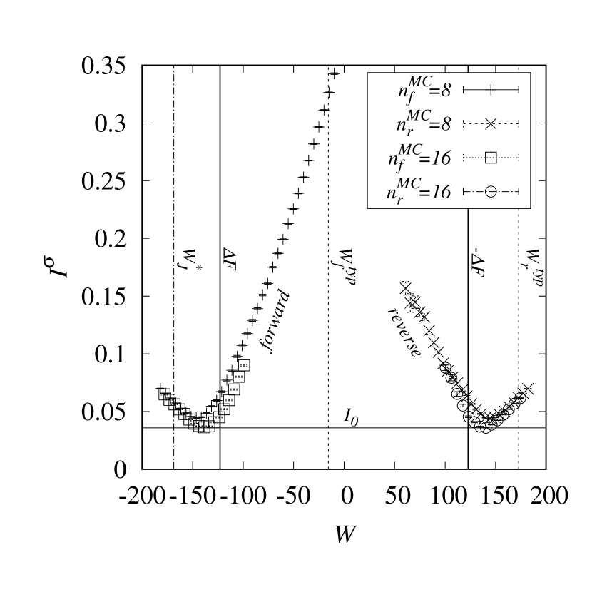
Figure 3: Integrated difference $I^{\sigma}$ between equilibrium and non-equilibrium overlap profiles at $T=1$, for forward (left) and backward (right) processes. For 16 sweeps the data is only partially shown, for better visibility. The horizontal line indicates $I_{0}$, the value of $I^{\sigma}$ in equilibrium. Vertical lines indicate work values at (from left to right) the maximum $W_{\rm J}^{*}$ of the Jarzynski integrand, the free energy difference $\Delta F$, the maximum $W^{typ}_{f}$ of the forward process work distribution, the negative free energy difference $-\Delta F$ and the maximum point $W^{typ}_{r}$ of the reverse process work distribution.

We quantify the similarity $I^{\sigma}$ of the non-equilibrium processes to the equilibrium case by integrating over all force values $f$ the absolute difference of $\overline{\sigma}(f)$ between the equilibrium and non-equilibrium case, and average this integral over close-by values of $W$, i.e., obtaining $I^{\sigma}(W)$. The result is shown in Fig. 3. We observe rather larger differences for typical values of $W$, while near $W\approx\pm\Delta F$ the similarity is of the order of the similarity $I_{0}$ obtained by averaging $I^{\sigma}$ over many independent equilibrium processes, which represents the equilibrium fluctuations. Also the forward processes sampled for work values near the value $W_{J}^{*}\approx-170$ where the Jarzynski integrand $P(W)e^{-W/T}$ peaks (see SM) exhibit a high similarity to the equilibrium case. Note that for the reverse process, the value of $W_{J}^{*}$ occurs outside our sampled region, thus we do not have processes for this case. For the slower case of $n_{\rm MC}=16$ sweeps, i.e., a bit nearer to equilibrium, the location minimum moves closer to $\Delta F$ and even decreases in height towards the equilibrium value $I_{0}$.

Thus, our results show that the rare processes near $W=\pm\Delta F$ do not only have similar work values like the equilibrium processes, they exhibit also very similar sequences, as function of the force $f$, of sampled structures. We obtained a similar result when considering force-extension curves, see SM.

Discussion — We studied RNA unfolding and refolding in equilibrium and in non-equilibrium. For the non-equilibrium case, by using sophisticated large-deviation algorithms, we could access a large range of the support of the probability distribution for the work. This allowed us to confirm the theorems of Crooks and Jarzynski over several dozens decades in probability. Furthermore, we analyzed the trajectories in force-extension as well as in secondary-structure space conditioned to various values of $W$. We observe that near the most relevant, but very improbable, values of $W$, the sampled trajectories reach a high similarity with true equilibrium. Thus, the study here does not depend on assigning a time-dependent weight to the trajectories, the selection is solely by the total work performed during the process and suitably evaluating fluctuation theorems. Also no other particular similarity to equilibrium is enforced explicitly by our procedure. Our approach and results may open a pathway to learning not only about equilibrium characteristic scalar numbers from non-equilibrium measurements, but even investigating near equilibrium dynamics by performing very fast but biased non-equilibrium simulations. We anticipate that similar studies are feasible and useful for many different types of systems.

For further studies, one could also extend the approach, by storing the configurations of the close-to-equilibrium $W\approx\Delta F$ generated rare trajectories. Starting with these configurations one could perform additional equilibrium simulations at fixed force values, i.e., without performing work, in the hope to get quickly close or even up to equilibrium. We have run some test simulations which show that one can indeed get even much closer to the equilibrium behavior by applying these add-on equilibration, apparently perfectly with respect to the force-extension curves, but this also depends on the temperature. Here more studies are needed, in particular a comparison of how good one can equilibrate by just using secondary-structure MC simulations when starting with empty configurations. Also it would be very interesting to see how these results depend of the actual RNA sequence and the corresponding energy landscape.

I Supplemantary Material

I.1 RNA secondary structure model

Each RNA molecule is a linear chain $\mathcal{R}=(r_{i})_{i=1,\dots,L}$ of bases, also called residues, with $r_{i}\in\{\mathrm{A,C,G,U}\}$ and $L$ is the length of the sequence. For a given sequence $\mathcal{R}$ of bases the secondary structure can be described by a set $\mathcal{S}$ of pairs $(i,j)$ (with the convention $1\leq i<j\leq L$), meaning that bases $r_{i}$ and $r_{j}$ are paired. For convenience, we also use $s(i)=j$ if $i$ is paired to $j$, which implies $s(j)=i$, and $s(i)=0$ if $i$ is not paired. We only allow Watson-Crick base pairs. These are formed by hydrogen bonds between complementary pairs of bases, i.e., A-U and C-G. Formally, this means for A-U either $r_{i}=$A and $r_{j}=$U or vice versa, correspondingly for the C-G pair. Two restrictions are used: (i) We exclude so called pseudo-knots, that means, for any $(i,j),(i^{\prime},j^{\prime})\in\mathcal{S}$, either $i<j<i^{\prime}<j^{\prime}$ or $i<i^{\prime}<j^{\prime}<j$ must hold, i.e., we follow the notion of pseudo knots being more an element of the tertiary structure Tinoco and Bustamante (1999). (ii) Between two paired bases a minimum distance is required: $|j-i|>s$ is required, granting some flexibility of the molecule (here $s=2$).

Every secondary structure $\mathcal{S}$ is assigned a certain energy $E(\mathcal{S})$, we do not explicitly indicate the dependence on the sequence $\mathcal{R}$. This energy is defined by assigning each pair $(i,j)$ a certain energy $e(r_{i},r_{j})$ depending only on the kind of bases.

Furthermore there is a contribution arising from the external force $f$ which stretches the chain to its extension $n(\mathcal{S})$, as introduced previously Müller et al. (2002). Thus, $n(\mathcal{S})$ is composed of a length of two units for each globule in the chain plus the number of bases in the free part, i.e., outside any globule. This is illustrated in Fig. 4.

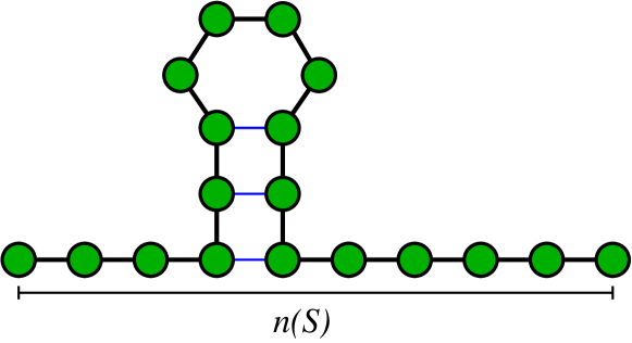
Figure 4: (color online) An example for a RNA secondary structure with one globule and a line indicating the extension $n(\mathcal{S})$ of the folded RNA. Circles denote bases, thick black lines links between consecutive bases, and thin blue lines hydrogen bonds between complementary bases.

The total energy is the sum over all pairs plus the interaction with the external force

$$E(\mathcal{S})=\sum_{(i,j)\in\mathcal{S}}e(r_{i},r_{j})-n(\mathcal{S})\,f\,.$$ (1)

By choosing $e(r,r^{\prime})=+\infty$ for non-complementary bases $r,r^{\prime}$ pairings of this kind are suppressed. Here we use the most simple energy model, i.e., $e(r,r^{\prime})=-1$ for complementary bases A-U and C-G.

I.2 Calculation of partition functions

The partition function $Z_{i,j}$ ($i\leq j$) for sub sequence $r_{i}\ldots r_{j}$ at inverse temperature $\beta=1/T$ without external force and without length constraints, obeying the minimum distance $s$ between two paired bases, is given by

$$Z_{i,j} =1\qquad\text{for}\quad j-i\leq s$$

$$Z_{i,j} =Z_{i,j-1}$$

$$+\sum_{k=i}^{j-s-1}Z_{i,k-1}e^{-\beta e(r_{k},r_{j})}Z_{k+1,j-1}\qquad\text{else}$$ (2)

All $O(L^{2})$ values of $Z_{i,j}$ can be conveniently calculated Nussinov et al. (1978) by a dynamic programming approach, i.e. starting with $Z_{i,i}$ and continuing with increasing values of $j-i$. Since most contributions involve a sum of $O(L)$ terms, the algorithm has a running time of $O(L^{3})$.

In order to include the interaction with the external force, one needs additionally the partition function $Q_{1,j,n}$ of the sub sequence $r_{1}\ldots r_{j}$ such that the extension is fixed to the value $n$, with $n\leq j$. We include the fixed index 1 for matching with the notation for $Z_{i,j}$,

Our approach follows the lines of a corresponding methods Gerland et al. (2001); Müller et al. (2002) for calculation of partition functions and ground state energies of RNA secondary structures subject to an external force. The partition function reads :

$$Q_{1,1,1}= 1$$

$$Q_{1,j,1}= 0\qquad\text{for}\quad j>1,$$

$$Q_{1,2,2}= Z_{1,2}$$

$$Q_{1,j,2}= 0\qquad\text{for}\quad 2<j\leq s+1$$ (3)

$$Q_{1,j,2}= e^{-\beta e(r_{1},r_{j})}Z_{2,j-1}\qquad\text{for}\quad j>s+1$$

$$Q_{1,j,n}= Q_{1,j-1,n-1}+\qquad\qquad\text{for}\quad n>2,j\geq n$$

$$\sum_{k=n-1}^{j-s-1}Q_{1,k-1,n-2}e^{-\beta e(r_{k},r_{j})}Z_{k+1,j-1}\,.$$

Also all these partition functions can be conveniently calculated by dynamic programming in time $O(L^{3})$.

This allows us to calculate the partition function with force for sub sequence $r_{1},\ldots,r_{j}$ by

$$\tilde{Z}_{1,j}(f)=\sum_{n=1}^{j}Q_{1,j,n}e^{\beta nf}\,.$$ (4)

Note that the case $n=0$ can not occur and the case $n=1$ corresponds only to one single base.

I.3 Sampling secondary structures

The availability of the above partition functions allows us to sample secondary structures in the presence of an external force directly, i.e. rejection free, also in polynomial time. The approach is an extension of the zero-force algorithm Higgs (1996) to the case $f\geq 0$.

For sampling a structure, the following probabilities are needed. The probability $p_{i,j,k}^{p}$ that for sub sequence $r_{i},\ldots,r_{j}$, without the presence or influence of a force, base $j$ is paired to base $k$ with $i\leq k<j$ and $j-k>s$ is given by

$$p_{i,j,k}^{p}=\frac{Z_{i,k-1}e^{-\beta e(r_{k},r_{j})}Z_{k+1,j-1}}{Z_{i,j}}\,.$$ (5)

For $j-k\leq s$, this probability is zero. The probability that base $j$ is not paired is given by

$$p_{i,j}^{u}=\frac{Z_{i,j-1}}{Z_{i,j}}\,.$$ (6)

The probability $\tilde{p}_{1,j,k}^{p}(f)$ that for sub sequence $r_{1},\ldots,r_{j}$, with the presence of a force $f$, base $j$ is paired to base $k$ with $1\leq k<j$ and $j-k>s$ is given by

$$\tilde{p}_{1,j,k}^{p}(f)=\frac{\tilde{Z}_{1,k-1}(f)e^{-\beta e(r_{k},r_{j})+\beta 2f}Z_{k+1,j-1}}{\tilde{Z}_{1,j}(f)}$$ (7)

For $j-k\leq s$, this probability is zero. The probability that base $j$ is not paired is given by

$$\tilde{p}_{1,j}^{u}(f)=\frac{\tilde{Z}_{1,j-1}(f)e^{\beta f}}{\tilde{Z}_{1,j}(f)}.$$ (8)

The sampling of a structure is now performed as follows. Each time one starts for the full sequence $r_{1},\ldots,r_{L}$ by considering the case with force $f$:

• Case with force $f$ for sub sequence $r_{1},\ldots,r_{j}$

  Base $j$ is paired to one of the bases $k=1,\ldots,j-s-1$ with probability $\tilde{p}_{1,j,k}^{p}(f)$, respectively, and remains unpaired with probability $\tilde{p}_{1,j}^{u}(f)$.

  Now, if base $j$ has been paired to base $k$, recursively the sequence $r_{1},\ldots,r_{k-1}$ is treated in the same way (case with force $f$) and the sub sequence $r_{k+1},\ldots,r_{j-1}$ is treated as described in the case without force.

  If base $j$ has not been paired, the sequence $r_{1},\ldots,r_{j-1}$ is treated in the same way (case with force $f$).

• Case without force for sub sequence $r_{i},\ldots,r_{j}$

  Base $j$ is paired to one of the bases $k=i,\ldots,j-s-1$ with probability $p_{i,j,k}^{p}$, respectively, and remains unpaired with probability $p_{i,j}^{u}$.

  Now, if base $j$ has been paired to base $k$, recursively the sequence $r_{i},\ldots,r_{k-1}$ and $r_{k+1},\ldots,r_{j-1}$ are treated in the same way (case without force).

  If base $j$ has not been paired, the sequence $r_{1},\ldots,r_{j-1}$ is treated in the same way (case without force).

In this way, each time a structure is independently drawn according to the Boltzmann distribution, i.e., the algorithm constitutes ideal sampling.

I.4 Folding and Unfolding Algorithm

The algorithm to determine the work for a given sequence $\mathcal{R}$ works as follows: First, a secondary structure is drawn in equilibrium at some given initial value $f_{0}$ of the force and for RNA temperature $T$. Then a Monte Carlo (MC) simulation allowing to change the secondary structure with total of $n_{\rm MC}$ sweeps is performed while the force parameter $f$ is increased or reduced depending on $\Delta f$. One sweep consist of $L^{2}/2$ Monte Carlo steps. During the MC simulation, $n_{\rm force}$ times the force is increased by $\Delta f$. For the individual MC steps, each time two random residues $i$ and $j$ are selected. If these are already paired to each other, the pair is removed, i.e., the bond broken, with the usual Metropolis probability $p_{\rm Metr}=\min\{1,\exp(-\beta\Delta E)\}$ determined by the energy change $\Delta E=-e(r_{i},r_{j})$. Note that we use negative pair energies, thus we have always $p_{\rm Metr}=\exp(\beta e(r_{i},r_{j}))$. In case of two non-bonded bases, they will be paired if they are complementary, and if they have a distance larger than $s$, and if no pseudo-knots would be created. The configuration is not changed when just one of the selected bases is already bounded, since a base can only connect to a single other one. The random numbers which are used during the MC simulation are generated before a call to the subroutine and stored in a vector $\xi$. In this way, all the randomness is removed outside this subroutine Crooks and Chandler (2001), for a reason we will present in the next section. Note that all other parameters like $\mathcal{R}$, $T$ etc. remain the same during a simulation, thus the work obtained during a unfolding or refolding is a deterministic function of $\xi$:

algorithm $W(\xi)$
begin
	draw for $\mathcal{R}$ an equilibrium structure $\mathcal{S}$ at
		initial force $f_{0}$ and RNA temperature $T$
	$f=f_{0}$
	$W=0$
	for $j=0,\cdots,n_{\rm force}$
	begin
		perform $L^{2}n_{\rm MC}/(2n_{\rm force})$ MC-Steps:
		begin
			select two random residues $l,m\in\{1,\ldots,L\}$
			if $(l,m)\in\mathcal{S}$, remove pair with prob. $p_{\rm Metr.}$
			else if $(l,m)$ is allowed set $\mathcal{S}=\mathcal{S}\cup\left\{(l,m)\right\}$
		end
		$f=f+\Delta f$
		$W=W-n(\mathcal{S})\Delta f$
	end
	return($W$)
end

The vector $\xi=(\xi_{1},\xi_{2},\ldots,\xi_{K})$ contains $K=L-1+3L^{2}n_{\rm MC}/2$ random numbers which are uniformly distributed in $[0,1]$. These are all random numbers that are needed to perform one full unfolding or refolding simulation. Each random number has a specific fixed purpose. The first $L-1$ entries are required to sample an configuration from the partition function, where an individual random number is utilized to determine if base $j\in[2,\dots,L]$ is either connected to base $k\in[1,\dots,j-s-1]$ or unconnected. Not all these $L-1$ random numbers are necessarily used during a specific sampling process, e.g., if for base $j$ the remaining sub sequence for a potential pairing partner is too small. In this case, the corresponding random number is just ignored, The subsequent MC steps need three random numbers each, two for selecting a pair and potentially one more, if the Metropolis criterion is used. If not, the third random number is also ignored, respectively. This results in a number of $3L^{2}n_{\rm MC}/2$ additional entries in $\xi$.

Note that more efficient Monte Carlo algorithms for RNA secondary structures exists Flamm et al. (2000); Dykeman (2015), which are event-driven Gillespie algorithms. Also they take as possible Monte Carlo moves only allowed moves into account, i.e., either pairs are removed, or only allowed pairs are proposed, avoiding non-complementary base pairs or pseudo knots. This requires keeping track of the allowed moves, which also generates quite some overhead in computation and it also involves the calculation of necessary corrections factors due to the varying number of accessible neighboring secondary structure configurations, in order to guarantee detailed balance. Also, the Gillespie nature of these algorithms make the use of random numbers dependent on the history of previous events. Nevertheless, for the present application, the work process is embedded into another higher-level Monte-Carlo simulation, see below. For a good performance of the higher-level MC simulation this requires that for each entry of the vector a specific purpose is assigned, as presented above. if this requirement is met, small changes to $\xi$ yield typically small, i.e., not too “chaotic” changes in the resulting work $W=W(\xi)$. This is the case with the present algorithm.

I.5 Large-deviation approach

Now we explain how the work simulations can be performed, such that also the tails of the work distribution $P(W)$ with potentially very small probabilities can be obtained. The method has been introduced for the Ising model Hartmann (2014), where more details are given. Here we review only the general idea and present the specific details for our study.

As mentioned in the previous section, for a given sequence $\mathcal{R}$, temperature $T$ and the other parameters, which are all kept fixed for a set of simulations, the outcome of the unfolding or refolding process is solely determined by the random values contained in the vector $\xi$. Thus, to perform a standard simple sampling simulation, one could each time draw a random vector $\xi$ with each entry being a pseudo random number uniformly distributed in $[0,1]$. This results in one work value $W$ which sampled from the true distribution. Thus, if one repeats the simple sampling many times, one can collect many work values and calculate a histogram to approximate the full distribution. Nevertheless, running the simple sampling $K$ times, will one only allow to resolve probabilities larger or equal $1/K$ in the histogram.

In order to access to work distribution down to very small probabilities, we did the following: We used a Markov chain Monte Carlo (MCMC) simulation where the states of the simulation are represented by samples $\xi^{(t)}$ of the random vectors used to drive the RNA unfolding or folding simulations. Thus, each state of the Markov chain corresponds to exactly one instance of a full process consisting of starting with an initial state in equilibrium and performing a, typically fast, non-equilibrium process during which the force is changed, the system has a bit of time to relax between two force changes, and a work value $W=W(\xi^{(t)})$ is obtained in the end. Therefore, the MCMC simulation takes place on a higher level than the unfolding or refolding simulations. Now, the main idea is to include a bias in the MCMC simulation, which involves a Metropolis acceptance depending on the change in the resulting work.

To be more precise, say we have the current state $\xi^{(t)}$ with work $W^{(t)}=W(\xi^{(t)})$ in the MCMC simulation. First, we generate a trial state $\xi^{\prime}$, which we obtain by copying $\xi^{(t)}$ and then redrawing a number $n_{\xi}<K$ of randomly selected entries from the $K$ entries of $\xi^{(t)}$. Next, we perform a complete work process for $\xi^{\prime}$, which results in the measured work $W^{\prime}=W(\xi^{\prime})$. Now, the trial state is accepted, i.e., $\xi^{(t+1)}=\xi^{\prime}$ with Metropolis probability $\tilde{p}_{\rm Metr}=\min\{1,\exp(-\Delta W/\Theta)\}$, where $\Delta W=W^{\prime}-W^{(t)}$ is the change in work and $\Theta$ is a temperature-like control parameter. Otherwise, the trial state is rejected, i.e., $\xi^{(t+1)}=\xi^{(t)}$. Note we aim at an empirical acceptance rate around 0.5 such that $n_{\xi}$ is typically small for small values of $\Theta$ and larger for larger values of $\Theta$. Actual values are given below.

Since the setup of the MCMC simulation is like any standard MCMC approach for a system coupled to a heat bath, only that we have replaced the energy by the work and use $\Theta$ for the temperature, it is obvious the our approach will sample the true work distribution but including a bias which is exactly the Boltzmann factor $\sim\exp(-W/\Theta)$. As usual, one has to discard the initial phase of the Markov chain, i.e., the equilibration phase, and to draw sample values only at suitable large time intervals. Thus, one can in principle perform simulations for a given value of $\Theta$, measure a histogram approximating the biased distribution $P_{\Theta}(W)\sim P(W)\exp(-W/\Theta)$, and obtain an estimate, up to the normalization constant, for the true distribution $P(W)$ by multiplication with $\exp(+W/\Theta)$. Note that, technically, to obtain the distribution over a large range of the support, one needs to perform simulations at several suitably chosen values of the control temperature $\Theta$, obtain the normlization constants for all measured histograms and combine them into one single finally normalized histogram Hartmann (2002). Details, in particular for the case of the work distribution of on Ising model in an external field, can be found elsewhere Hartmann (2014). This approach has already been applied to other non-equilibrium processes like the Kardar-Parisi-Zhang model Hartmann et al. (2018) or traffic flows Staffeldt and Hartmann (2019).

I.6 Example secondary structures

In Fig. 5 equilibrium secondary structures are shown. It becomes apparent how the extension increases with the force parameter $f$.

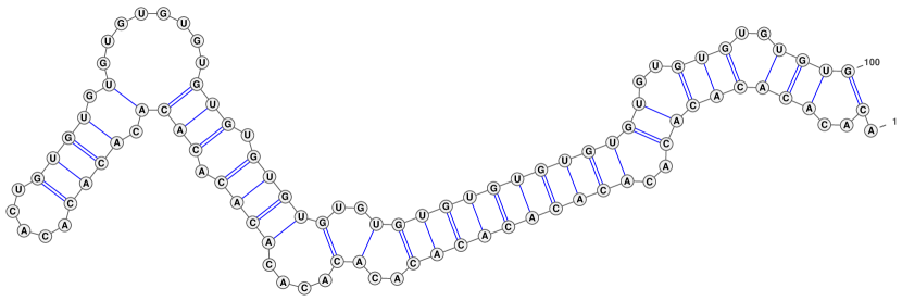
Figure 5: Exemplary equilibrium secondary structures at $T=1$ for different forces. Top: $f=0$. Middle: $f=0.805$. Bottom: $f=2$. Drawn with the VARNA package Darty et al. (2009).

I.7 Simulation parameters

For all unfolding and refolding processes, the force was increased from $f_{0}=0$ to $f_{\max}=2$ and vice versa, with 400 steps each. Thus, the change of the force was $\Delta f=\pm 0.005$. Table 1 shows the other simulation parameters we have used.

$T$	$n_{\rm MC}$	$f$	$n_{\Theta}$	$\Theta_{\min}$	$\Theta_{\max}$	$n_{\xi,\min}$	$n_{\xi,\max}$	$t_{\rm ld}/10^{8}$
0.3	8	$0\to 2$	17	0.6	7	938	$9\times 10^{4}$	5.44
0.3	8	$2\to 0$	10	0.4	2	1587	$6\times 10^{4}$	4.05
0.3	16	$0\to 2$	18	0.6	8	1407	$12\times 10^{4}$	2.50
0.3	16	$2\to 0$	10	0.4	2	2500	$9\times 10^{4}$	1.82
1	8	$0\to 2$	11	0.8	10	354	$6\times 10^{4}$	6.95
1	8	$2\to 0$	13	1	5	1350	$6\times 10^{4}$	2.81
1	16	$0\to 2$	11	0.8	10	938	$75\times 10^{2}$	4.41
1	16	$2\to 0$	10	0.8	5	2344	$12\times 10^{4}$	2.35

Table 1: Simulation parameters for different temperatures $T$ and for different process speeds $n_{\rm MC}$ and unfolding ($f=0\to 2$) and refolding ($f=2\to 0$) processes. For the large-deviation MCMC simulation $n_{\Theta}$ different values of the temperature-like parameter $\Theta\in[\Theta_{\min},\Theta_{\max}]$ were considered. In each MCMC step a number $n_{\xi}\in[n_{\xi,\min},n_{\xi,\max}]$ of entries from the vectors $\xi$ of random numbers are changed. For the lowest value of $\Theta$ we have $n_{\xi}=n_{\xi,\min}$, for the largest $n_{\xi}=n_{\xi,\max}$, for the others in between. The total number of MCMC steps in the large-deviation simulation was always larger than the given values $t_{\rm ld}$, the actual values depending on the value of $\Theta$ and on the available computing time on the computing cluster, respectively. The longest running time occurred for the unfolding (forward) process $T=1,n_{\rm MC}=8$ and took $t_{\rm ld}=14.5\times 10^{8}$ steps.

I.8 Work distributions

In Fig. 6 the work distributions for $T=1$ of the slower process, at total of 16 MC sweeps per process, are shown. The results look similar to the 8 sweeps case, but the distributions are located a bit closer to each other here, such that the intersections of $P(W)$ and $P_{\rm rev}(-W)$ occur at higher probability. In the inset of Fig. 6 the corresponding rescaled distribution for the reverse process is shown. Also for 16 MC sweeps a good agreement with the distribution for the forward process is visible, over more than 20 decades.

Figure 6: Plain and mirrored work distributions for $T=1$ and 16 sweeps of the forward and reverse process, respectively. They intersect near $W=\Delta F$, which is the exact value and indicated by the vertical line. The inset shows the same plot but with the distribution for the reverse process (cross symbols) rescaled as $P_{\rm rev}(W)\exp(-(\Delta F-W)/T)$, according to the equation of Crooks, yielding a good agreement with $P(W)$.

In Figs. 7 and 8 the corresponding results for the lower temperature $T=0.3$ are shown. Again, Crooks theorem is confirmed with high precision, where here the distribution was even obtained down to probabilities as small as $10^{-46}$.

Figure 7: Plain and mirrored work distributions for $T=0.3$ and 8 sweeps of the forward and reverse process, respectively. They intersect near $W=\Delta F$, which is the exact value and indicated by the vertical line. The inset shows the same plot but with the distribution for the reverse process (cross symbols) rescaled as $P_{\rm rev}(W)\exp(-(\Delta F-W)/T)$, according to the equation of Crooks, yielding a good agreement with $P(W)$.

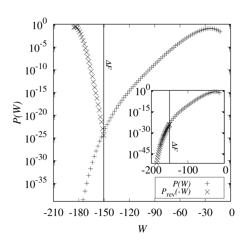
Figure 8: Plain and mirrored work distributions for $T=0.3$ and 16 sweeps of the forward and reverse process, respectively. They intersect near $W=\Delta F$, which is the exact value and indicated by the vertical line. The inset shows the same plot but with the distribution for the reverse process (cross symbols) rescaled as $P_{\rm rev}(W)\exp(-(\Delta F-W)/T)$, according to the equation of Crooks, yielding a good agreement with $P(W)$.

I.9 Jarzynski Integrand

The integrand of $\langle e^{-W/T}\rangle=\int dWP(W)e^{-W/T}$ is shown in Fig. 9, for $T=1$, $n_{\rm MC}=8$ and forward and reverse work processes, respectively. The point where the integrand peaks is exponentially relevant and can be used to approximate the integral. This, together with its probability, determines according to Jarzynski’s equation the free energy difference.

Figure 9: Jarzynski integrand of the forward process for 8 sweeps at $T=1$. Inset: Same for the reverse process, in which the maximum is not reached. Error bars are smaller than symbol sizes.

I.10 Overlap

For two secondary structures $\mathcal{S}$ and $\mathcal{S^{\prime}}$ and the equivalent notations $\{s(i)\}$ and $\{s^{\prime}(i)\}$ for the pairing partners of the residues (0 if not paired), we define the overlap

$$\sigma(\mathcal{S},\mathcal{S}^{\prime})=\frac{1}{L}\sum_{i=1}^{L}\delta_{s(i),s^{\prime}(i)}\,$$ (9)

where the Kronecker delta is given by $\delta_{k,l}=1$ if $k=l$ and $\delta_{k,l}=0$ else. Thus, the overlap equals one when $\mathcal{S},\mathcal{S}^{\prime}$ denote the same secondary structure, and zero when they are completely different.

I.11 Force-extension curves

In addition to the overlap profiles $\sigma(f)$ we have presented in the main paper, we also used force extension curves (FECs) $n(f)$ to compare processes for equilibrium and non-equilibrium situations. Note that the extension $n(\mathcal{S})$ of a structure can be very much influenced by single base pairs. Thus two processes, which look very similar on the level of secondary structures, can be very different with respect to force-extension curves.

Figure 10: Top left: Mean FECs, in equilibrium, for typical forward processes and for work values near $\Delta F$, for two different number of $n_{\rm MC}$ of sweeps at $T=1$. Top right: Samples of such single FECs in equilibrium. Bottom left: samples of non-equilibrium FECs with $n_{\rm MC}=8$ for $W$ near $\Delta F$. Bottom right: samples of typical non-equilibrium FECs, i.e., where $W\gg\Delta F$, with $n_{\rm MC}=8$. The solid line represents always the mean equilibrium FEC.

Samples for equilibrium and non-equilibrium FECs for forward processes, along with corresponding averages, are shown in Fig. 10. For the equilibrium case, a sigmoidal form can be observed, with some fluctuations, with a strong change near the critical force value where the folding-unfolding transition takes place Müller et al. (2002). For the non-equilibrium case, the typical FECs, i.e., with typical work values $W$ far from $\Delta F$, agree only for small values of $f$, i.e., in the initial phase of the process. On the other hand, the rare processes with $W$ close to $\Delta F$, where five different examples are shown here, are much more similar to the equilibrium FECs. Here, differences appear mainly near the critical folding-unfolding force.

Figure 11: Top left: Mean FECs, in equilibrium, for typical reverse processes and for work values near $\Delta F$, for two different number of $n_{\rm MC}$ of sweeps at $T=1$. Top right: Samples of such single FECs in equilibrium. Bottom left: samples of non-equilibrium reverse FECs with $n_{\rm MC}=8$ for $W$ near $\Delta F$. Bottom right: samples of typical non-equilibrium reverse FECs, i.e., where $W\gg\Delta F$, with $n_{\rm MC}=8$. The solid line represents always the mean equilibrium FEC.

Samples for equilibrium and non-equilibrium FECs for backward processes, along with corresponding averages, are shown in Fig. 11. The results correspond to the forward case, but the processes with typical values of $W$ agree well with the average equilibrium FEC only for large values of $f$ but not for small values of $f$. But this means they also agree in the initial phase of the process, before the critical folding-unfolding force value is reached. The FECs for work values $W\approx\Delta F$ are also for reverse processes much more similar to the equilibrium case than typical reverse processes.

These results are confirmed by averaging the absolute value of the differences between one FEC $n(f)$ and the mean equilibrium FEC $\overline{n}_{Eq}(f)$ over all available values of the force $f$, i.e., calculating $I^{n}=[\frac{1}{n_{\rm f}}\sum_{f}|n(f)-\overline{n}_{Eq}(f)|]$ where the average $[\ldots]$ is over different realisations of $n(f)$. Even when considering equilibrium FECs for $n(f)$, respectively, there is some variation reflected by a non-zero average value $I_{0}$. When using non-equilibrium FECs, with a specified binned value of $W$, one sees stronger differences, as visible in Fig. 12. Similar to $I^{\sigma}$, the closest agreements between non-equilibrium and equilibrium are seen near $W\approx\Delta F$. In contrast to $I^{\sigma}$ the level of the equilibrium fluctuations is not reached for the measurable quantity FEC.

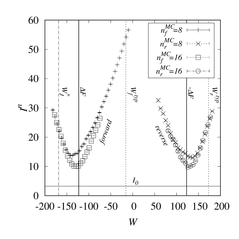
Figure 12: Integrated extension difference $I^{n}$ between equilibrium and non-equilibrium at $T=1$. For 8 sweeps the entire work range is plotted, where for 16 sweeps only a range around the minimum is shown, for better visibility. $I_{0}$, represented by a horizontal line, is the averaged value of $I^{n}$ when comparing always two equilibrium FECs. The left curves represent the forward, the right ones the reverse process. Vertical lines indicate work values at (from left to right) the maximum $W_{J}^{*}$ of the Jarzynski integrand , the free energy difference $\Delta F$, the maximum $W^{typ}_{f}$ of the forward process work distribution , the negative free energy difference $-\Delta F$ and the maximum point $W^{typ}_{r}$ of the reverse process work distribution.

References

- Jarzynski (1997a) C. Jarzynski, Phys. Rev. Lett. 78, 2690 (1997a).
- Crooks (1998) G. E. Crooks, J. Stat. Phys. 90, 1481 (1998).
- Kurchan (2007) J. Kurchan, JSTAT 2007, P07005 (2007).
- Seifert (2008) U. Seifert, Eur. Phys. J. B 64, 423 (2008).
- Sevick et al. (2008) E. M. Sevick, R. Prabhakar, S. R. Williams, and D. J. Searles, Ann. Rev. Phys. Chem. 59, 603 (2008).
- Jarzynski (2008) C. Jarzynski, Eur. Phys. J. B 64, 331 (2008).
- Esposito et al. (2009) M. Esposito, U. Harbola, and S. Mukamel, Rev. Mod. Phys. 81, 1665 (2009).
- Jarzynski (2011) C. Jarzynski, Annual Review of Condensed Matter Physics 2, 329 (2011).
- Seifert (2012) U. Seifert, Rep. Progr. Phys. 75 (2012), 10.1088/0034-4885/75/12/126001.
- Marsland III and England (2018) R. Marsland III and J. England, Rep. Progr. Phys. 81 (2018), 10.1088/1361-6633/aa9101.
- Hartmann (2015) A. K. Hartmann, Big Practical Guide to Computer Simulations (World Scientific, Singapore, 2015).
- Hummer and Szabo (2010) G. Hummer and A. Szabo, Proc. Natl. Acad. Sci. 107, 21441–21446 (2010).
- Evans et al. (1993) D. J. Evans, E. G. D. Cohen, and G. P. Morriss, Phys. Rev. Lett. 71, 2401 (1993).
- Evans and Searles (1994) D. J. Evans and D. J. Searles, Phys. Rev. E 50, 1645 (1994).
- Gallavotti and Cohen (1995a) G. Gallavotti and E. G. D. Cohen, Phys. Rev. Lett. 74, 2694 (1995a).
- Gallavotti and Cohen (1995b) G. Gallavotti and E. G. D. Cohen, J. Stat. Phys. 80, 931 (1995b).
- Kurchan (1998) J. Kurchan, J. Phys. A: Math. Gen. 31, 3719 (1998).
- Lebowitz and Spohn (1999) J. L. Lebowitz and H. Spohn, J. Stat. Phys. 95, 333 (1999).
- Maes (1999) C. Maes, J. Stat. Phys. 95, 367 (1999).
- Crooks (1999) G. E. Crooks, Phys. Rev. E 60, 2721 (1999).
- Crooks (2000) G. E. Crooks, Phys. Rev. E 61, 2361 (2000).
- Adib (2005) A. B. Adib, Phys. Rev. E 71, 056128 (2005).
- Jarzynski (1997b) C. Jarzynski, Phys. Rev. E 56, 5018 (1997b).
- Hummer and Szabo (2001) G. Hummer and A. Szabo, Proc. Nat. Acad. Sci. 98, 3658 (2001).
- Müller et al. (2002) M. Müller, F. Krzakala, and M. Mézard, Eur. Phys. J. E 9, 67–77 (2002).
- Hartmann (2002) A. K. Hartmann, Phys. Rev. E 65, 056102 (2002).
- Bucklew (2004) J. A. Bucklew, Introduction to rare event simulation (Springer-Verlag, New York, 2004).
- Dellago et al. (1998) C. Dellago, P. G. Bolhuis, F. S. Csajka, and D. Chandler, J. Chem. Phys. 108, 1964 (1998).
- Bolhuis et al. (2002) P. G. Bolhuis, D. Chandler, C. Dellago, and P. L. Geissler, Ann. Rev. Phys. Chem. 53, 291 (2002), pMID: 11972010.
- Giardinà et al. (2006) C. Giardinà, J. Kurchan, and L. Peliti, Phys. Rev. Lett. 96, 120603 (2006).
- Lecomte and Tailleur (2007) V. Lecomte and J. Tailleur, JSTAT 2007, P03004 (2007).
- Staffeldt and Hartmann (2019) W. Staffeldt and A. K. Hartmann, Phys. Rev. E 100, 062301 (2019).
- Hartmann et al. (2018) A. K. Hartmann, P. L. Doussal, S. N. Majumdar, A. Rosso, and G. Schehr, Europhys. Lett. 121, 67004 (2018).
- Hartmann (2014) A. K. Hartmann, Phys. Rev. E 89, 052103 (2014).
- Higgs (1996) P. G. Higgs, Phys. Rev. Lett. 76, 704 (1996).
- Burghardt and Hartmann (2005) B. Burghardt and A. K. Hartmann, Phys. Rev. E 71, 021913 (2005).
- Lorenz et al. (2011) R. Lorenz, S. H. Bernhart, C. Höner zu Siederdissen, H. Tafer, C. Flamm, P. F. Stadler, and I. L. Hofacker, Algor. Mol. Biol. 6, 26 (2011).
- Gerland et al. (2001) U. Gerland, R. Bundschuh, and H. T., Biophys J. 81, 1324 (2001).
- Nussinov et al. (1978) R. Nussinov, G. Pieczenik, J. R. Griggs, and D. J. Kleitman, SIAM J. Appl. Math. 35, 68 (1978).
- Mézard et al. (1987) M. Mézard, G. Parisi, and M. Virasoro, Spin glass theory and beyond (World Scientific, Singapore, 1987).
- Tinoco and Bustamante (1999) I. Tinoco and C. Bustamante, J. Mol. Biol. 293, 271 (1999).
- Crooks and Chandler (2001) G. E. Crooks and D. Chandler, Phys. Rev. E 64, 026109 (2001).
- Flamm et al. (2000) C. Flamm, W. Fontana, I. L. Hofacker, and P. Schuster, RNA 6, 325–338 (2000).
- Dykeman (2015) E. E. Dykeman, Nucleic Acids Research 43, 5708–5715 (2015).
- Darty et al. (2009) K. Darty, A. Denise, and Y. Ponty, Bioinformatics 25, 1974 (2009).