Conditional uniqueness of solutions to the Keller–Rubinow model for Liesegang rings
in the fast reaction limit

Abstract.

We study the question of uniqueness of weak solution to the fast reaction limit of the Keller and Rubinow model for Liesegang rings as introduced by Hilhorst et al. (J. Stat. Phys. 135, 2009, pp. 107–132). The model is characterized by a discontinuous reaction term which can be seen as an instance of spatially distributed non-ideal relay hysteresis. In general, uniqueness of solutions for such models is conditional on certain transversality conditions. For the model studied here, we give an explicit description of the precipitation boundary which gives rise to two scenarios for non-uniqueness, which we term “spontaneous precipitation” and “entanglement”. Spontaneous precipitation can be easily dismissed by an additional, physically reasonable criterion in the concept of weak solution. The second scenario is one where the precipitation boundaries of two distinct solutions cannot be ordered in any neighborhood of some point on their common precipitation boundary. We show that for a finite, possibly short interval of time, solutions are unique. Beyond this point, unique continuation is subject to a spatial or temporal transversality condition. The temporal transversality condition takes the same form that would be expected for a simple multicomponent semilinear ODE with discontinuous reaction terms.

1. Introduction

We study the question of uniqueness of weak solution to the fast reaction limit of the Keller and Rubinow model for Liesegang rings,

$$u_{t}=u_{xx}+\frac{\alpha\beta}{2\sqrt{t}}\,\delta(x-\alpha\sqrt{t})-p[x,t;u]\,u\,,$$ (1.1a)

$$u_{x}(0,t)=0\quad\text{for }t\geq 0\,,$$ (1.1b)

$$u(x,0)=0\quad\text{for }x>0$$ (1.1c)

where the precipitation function $$p[x,t;u] x t u$$ depends on , , and nonlocally on via

$$p[x,t;u]=H\biggl{(}\int_{0}^{t}(u(x,\tau)-u^{*})_{+}\,\mathrm{d}\tau\biggr{)}\,.$$ (1.1d)

Here, $H$ denotes the Heaviside function with the convention that $H(0)=0$ and $u^{*}$ denotes the supersaturation concentration.

The model was derived by Hilhorst et al. [12, 13], based on earlier work in [14, 15], from a three-component two-stage system of reaction-diffusion equations due to Keller and Rubinow [16] under the assumption that one of the first-stage reactants does not diffuse, that the lower threshold of criticality is zero, and that the reaction constant of the first-stage reaction is large. In the following, we shall refer to the reduced model (1.1) as the HHMO-model.

Hilhorst et al. [12, 13] introduced and proved existence of weak solutions to (1.1). Modulo technical details, weak solutions are pairs $(u,p)$ that satisfy (1.1a) integrated against a suitable test function such that

$$p(x,t)\in H\biggl{(}\int_{0}^{t}(u(x,\tau)-u^{*})_{+}\,\mathrm{d}\tau\biggr{)}$$ (1.2)

where $H$ denotes the Heaviside graph

$$H(y)\in\begin{cases}0&\text{when }y<0\,,\\ [0,1]&\text{when }y=0\,,\\ 1&\text{when }y>0\,,\end{cases}$$ (1.3)

subject to the additional requirement that $p(x,t)$ takes the value $0$ whenever $u(x,s)$ is strictly less than the threshold $u^{*}$ for all $s\in[0,t]$. This constraint can be stated as

$$p(x,t)\in\begin{cases}0&\text{ if }\sup_{s\in[0,t]}u(x,s)<u^{*}\,,\\ [0,1]&\text{ if }\sup_{s\in[0,t]}u(x,s)=u^{*}\,,\\ 1&\text{ if }\sup_{s\in[0,t]}u(x,s)>u^{*}\,.\end{cases}$$ (1.4)

The problem left open by [13] is the question of uniqueness of weak solutions to the HHMO-model. The main obstacle is that the precipitation term is neither Lipschitz continuous nor local in time. Moreover, it may not even be monotonic in the following sense. If $u_{1}$ and $u_{2}$ are weak solutions with associated precipitation functions $p_{1}$ and $p_{2}$, it is not clear whether

$$(p_{1}\,u_{1}-p_{2}\,u_{2})\,(u_{1}-u_{2})\geq 0$$ (1.5)

a.e. in space-time. An estimate of this form would imply uniqueness by standard energy methods. We remark that for other models involving phase transitions, e.g. for moist advection in models of the atmosphere with humidity and saturation [3, 18], monotonicity can be asserted. The behavior of the precipitation function is an instance of a one-sided non-ideal relay. In general, non-ideal relays switch from an “off-state” $0$ to the “on-state” $1$ when the input crosses a threshold $\mu$, and switches back to zero only when the input drops below a lower threshold $\lambda<\mu$. Here, the lower threshold is $\lambda=0$, so the relay never switches back. There are different ways of defining the behavior of non-ideal relays; see, e.g., the brief survey in [4]. The formulations differ in their behavior when the input reaches, but does not exceed the relay threshold. The three options described in [4] are: (i) The relay switches as soon as the threshold is reached [10, 11, 17, 20], (ii) the relay switches only when the threshold is exceeded, attributed to Alt [2], or (iii) may take intermediate values at the threshold subject to certain monotonicity constraints, which are referred to as a completed relay [1, 19]. All these formulations are “rate independent”, i.e., the state of the relay only depends on the past and present values of the input, but not on their rate of change. All rate-independent formulations have issues regarding their well-posedness in cases of non-transversal crossings of the threshold.

The uniqueness issue can be illustrated with a simple system of two ordinary differential equations, but extends to the case of spatially distributed relays, including the HHMO-model as a reaction-diffusion equation with precipitation. For simplicity, we translate the crossing of the critical threshold into the origin and look at the non-autonomous system

$$\dot{u}(t)=f(t)+u(t)+v(t)-p_{u}(t)\,,$$ (1.6a)

$$\dot{v}(t)=f(t)+u(t)+v(t)-p_{v}(t)\,,$$ (1.6b)

$$u(0)=v(0)=0\,.$$ (1.6c)

Here, $p_{u}$ and $p_{v}$ denote the precipitation condition (1.4) with $u^{*}=0$ for $u$ and $v$, respectively. If $p_{u}$ and $p_{v}$ are permitted to assume fractional values, there is no hope for uniqueness, so the question here is whether the restriction of $p_{u}$ and $p_{v}$ to binary values suffices to select a unique solution.

Let us first consider the case $f(t)=\tfrac{1}{2}$. In this case, the vector field without the precipitation terms is positive in both components at time $t=0$ when the threshold is touched; we speak of a transversal crossing. We see that both precipitation functions must switch from zero to one at that instant. Indeed, if none of the precipitation functions switches, the solution is $u(t)=v(t)=(\exp(2t)-1)/4>0$ on some interval of positive time, which violates (1.4). If one of the precipitation function switches, $p_{u}$ say, the solution is $u(t)=-t/2$, $v(t)=t/2$, so that the precipitation condition is still violated on some interval of positive time. So there is no choice and both must switch.

If, on the other hand, $f(t)=t$, the vector field without the precipitation terms is zero in both components at time $t=0$ when the threshold is touched; we speak of a non-transversal crossing. Again, it is easy to see that at least one of the precipitation functions must switch at $t=0$ for if not, both $u$ and $v$ will be positive for $t>0$, violating the precipitation condition (1.4). However, suppose that $p_{u}$ switches to $1$ at $t=0$, while $p_{v}$ remains zero. Then $u(t)=-t$ and $v(t)=0$, which is a feasible solution. Due to the symmetry, $p_{u}=0$ and $p_{v}=1$ also gives a feasible solution.

We remark that as soon as fractional values are permitted, there are further feasible solutions: in the transversal example, e.g. $p_{u}=p_{v}=\tfrac{1}{2}$ is feasible, in the non-transversal example, any convex combination $p_{u}=\lambda$ and $p_{v}=1-\lambda$ with $\lambda\in[0,1]$ gives a feasible solution. We believe that a better disambiguation criterion would permit fractional values of the precipitation function augmented by a suitable minimality condition. This, however, is not trivial and outside of the scope of this paper. For the present paper on the HHMO-model, we avoid this discussion altogether by proving that, on some positive interval of time, the precipitation function of a weak solution is essentially binary, i.e. binary except perhaps for values on a space-time set of measure zero.

Our results are the following. We identify two scenarios for non-uniqueness, “spontaneous precipitation” and “entanglement”. Spontaneous precipitation can be easily dismissed by an additional, physically reasonable criterion in the concept of weak solution. Entanglement is a scenario where there exists a point on the common precipitation boundary such that in every neighborhood of this point there are subregions where each one of two non-unique boundary curves is ahead of the other. To dismiss the second scenario, we perform a detailed study of the topological and analytic properties of the precipitation boundary. Our results are two-fold. First, there exists an initial interval of time where monotonicity in the sense of (1.5), hence uniqueness, holds true. Second, we state a transversality condition, namely that the temporal rate of change of concentration is non-degenerate at the precipitation boundary, which prevents entanglement and implies monotonicity, hence uniqueness. Our analysis is restricted to a region where the solution consists of a succession of distinct precipitation rings, the ring domain. In numerical simulations of a range of models, including the HHMO-model and the full Keller–Rubinow model, the ring domain appears to persist for only a finite interval of time, longer than our initial interval of uniqueness; breakdown of the ring domain is proved for a simplified version of the HHMO-model in [7]. After that, solutions may become topologically even more complex and our methods do not apply. For the simplified model in [7], a reduction of the problem to a scalar integral equation is possible and the question of uniqueness can be answered in the affirmative in a class of solutions that excludes accumulation of precipitation rings in reverse time [6]. For the HHMO-model itself, this reduction is not possible and the question remains open.

The paper is structured as follows. In Section 2, we review the concept of weak solutions, their basic properties, and show that there are weak solutions whose precipitation function is not changing at a point after the reactant source has passed. In Section 3, we introduce the “ring domain”, a non-empty region in which the solution can be characterized by distinct precipitation bands, and prove a number of topological and analytic properties of the precipitation boundary on the ring domain. In particular, we show that the precipitation function can be given a canonical form up to changes on space-time sets of measure zero. In Section 4 we present a boot-strap argument that guarantees existence and continuity of a classical time derivative away from the precipitation boundary and give a sufficient condition that ensures existence and continuity of the time derivative on the precipitation boundary as well. Finally, uniqueness is proved in Section 5, unconditionally up to a finite, possibly small time and under a temporal transversality condition on the entire ring domain.

2. Weak solutions

To begin, we note that without the precipitation term, (1.1) has the explicit solution

$$\psi(x,t)=\Psi\Bigl{(}\frac{x}{\sqrt{t}}\Bigr{)}$$ (2.1)

where

$$\Psi(\eta) =\frac{\alpha\beta\sqrt{\pi}}{2}\,\mathrm{e}^{\tfrac{\alpha^{2}}{4}}\cdot\begin{dcases}\operatorname{erfc}(\alpha/2)&\text{if }\eta\leq\alpha\,,\\ \operatorname{erfc}(\eta/2)&\text{if }\eta>\alpha\,.\end{dcases}$$ (2.2)

For further reference, we also define the standard heat kernel

$$\Phi(x,t)=\begin{dcases}\frac{1}{\sqrt{4\pi t}}\,\mathrm{e}^{-\tfrac{x^{2}}{4t}}&\text{if }t>0\,,\\ 0&\text{if }t\leq 0\,.\end{dcases}$$ (2.3)

In the following definition of weak solution, we follow [13, 8] and extend the spatial domain to the entire real line by even reflection. In the main body of the paper, however, it is easier to formulate all arguments and definitions exclusively on the first quadrant of the $x$-$t$ plane. Due to the implied even symmetry, we may still refer to the fields at $x<0$ when convenient, in particular when stating arguments based on the Duhamel principle.

Definition 1.

A weak solution to problem (1.1) is a pair $(u,p)$ satisfying

1. $u$ and $p$ are even in $x$, i.e. $u(x,t)=u(-x,t)$ and $p(x,t)=p(-x,t)$ for all $x\in\mathbb{R}$ and $t\geq 0$,

2. $u-\psi\in C^{1,0}(\mathbb{R}\times[0,T])\cap L^{\infty}(\mathbb{R}\times[0,T])$ for every $T>0$,

3. $p$ is measurable, defined pointwise, and satisfies (1.4),

4. $p(x,t)$ is non-decreasing in time $t$ for every $x\in\mathbb{R}$,

5. the relation

   $$\int_{0}^{T}\int_{\mathbb{R}}\varphi_{t}\,(u-\psi)\,\mathrm{d}y\,\mathrm{d}s=\int_{0}^{T}\int_{\mathbb{R}}\bigl{(}\varphi_{x}\,(u-\psi)_{x}+p\,u\,\varphi\bigr{)}\,\mathrm{d}y\,\mathrm{d}s$$ (2.4)

   holds for every $\varphi\in C^{1,1}(\mathbb{R}\times[0,T])$ that vanishes for large values of $|x|$ and for time $t=T$.

The following additional notation is used throughout the paper. We define

$$\mathcal{P}=\{(x,t)\colon\alpha^{2}\,t=x^{2}\}$$ (2.5a)

to denote the parabola on which the point source moves, and write

$$D_{o} =\{(x,t)\colon 0<x^{2}<\alpha^{2}\,t\}\,,$$ (2.5b)

$$D_{u} =\{(x,t)\colon 0<\alpha^{2}\,t<x^{2}\}$$ (2.5c)

to denote the open region of the upper half-plane over and under the parabola $\mathcal{P}$, respectively. Moreover, we formalize the notion of precipitation ring and interring (or gap) as follows.

Definition 2.

The interval $[a,b]$ with $b>a>0$ is a ring if the set

$$\{(y,s)\colon y\in[a-\varepsilon_{1},b+\varepsilon_{2}],\alpha^{2}\,s\geq y^{2},\,p(y,s)<1\}\subset\mathbb{R}^{2}$$ (2.6)

with non-negative $\varepsilon_{1}$, $\varepsilon_{2}$ has measure zero if and only if $\varepsilon_{1}=\varepsilon_{2}=0$.

When $b>a=0$, the interval $[0,b]$ is a ring if the set

$$\{(y,s)\colon y\in[0,b+\varepsilon_{1}],\alpha^{2}\,s\geq y^{2},\,p(y,s)<1\}\subset\mathbb{R}^{2}$$ (2.7)

with non-negative $\varepsilon_{1}$ has measure zero if and only if $\varepsilon_{1}=0$.

Remark 1.

If $[a,b]$ is a ring and $x\in[a,b]$—we say that “$x$ is contained in a ring”—then $\max_{s\in[0,x^{2}/\alpha^{2}]}u(x,s)\geq u^{*}$. For if not, by continuity of $u$, there would be a neighborhood of the line segment $\{x\}\times[0,x^{2}/\alpha^{2}]$ on which $u<u^{*}$. But for a weak solution satisfying property (P), this means that $x$ cannot be contained in a ring. In Section 3 we shall show that $\max_{s\in[0,x^{2}/\alpha^{2}]}u(x,s)=u^{*}$ only if the maximum is taken exclusively on $\mathcal{P}$, we then speak of a degenerate precipitation boundary point.

Definition 3.

The interval $[a,b]$ with $b>a>0$ is an interring if the set

$$\{(y,s)\colon y\in[a-\varepsilon_{1},b+\varepsilon_{2}],\,p(y,s)>0\}\subset\mathbb{R}^{2}$$ (2.8)

with non-negative $\varepsilon_{1}$, $\varepsilon_{2}$ has measure zero if and only if $\varepsilon_{1}=\varepsilon_{2}=0$.

When $0<a$, the interval $[a,\infty)$ is an interring if the set

$$\{(y,s)\colon y\geq a-\varepsilon,p(y,s)>0\}\subset\mathbb{R}^{2}$$ (2.9)

with non-negative $\varepsilon$ has measure zero if and only if $\varepsilon=0$.

When $u^{*}\geq\Psi(\alpha)$, the so-called subcritical or marginal cases, it is not possible to have a recurrent pattern of rings and interrings. In these cases, weak solutions have a simple structure which is completely described by [8, Theorems 4 and 5]. Therefore we focus on the interesting supercritical case where $u^{*}<\Psi(\alpha)$. In this case, the following lemma asserts that at least a first precipitation ring always exists.

Lemma 4 (Existence of a first precipitation ring).

Every weak solution to equation (1.1) with supercritical precipitation threshold $u^{*}$ has at least one precipitation ring of width at least $X_{1}\geq L$, where

$$L=\sqrt{\frac{\Psi(\alpha)-u^{*}}{\Psi(\alpha)}}\,.$$ (2.10)

In particular, there is no interring of the form $[0,d]$.

Proof.

First, recall [13, Lemma 3.5], which states that

$$u(x,t)\geq\psi(x,t)-\Psi(\alpha)\,t\,.$$ (2.11)

Second, note that there exists a $t^{*}>0$ such that

$$u^{*}=\Psi(\alpha)-\Psi(\alpha)\,t^{*}\,.$$ (2.12)

Hence, (2.11) implies that if $(x,t)\in\mathcal{P}$ with $t<t^{*}$, then

$$u(x,t)\geq\psi(x,t)-\Psi(\alpha)t>\Psi(\alpha)-\Psi(\alpha)t^{*}=u^{*}\,.$$ (2.13)

In other words, $u$ is strictly greater than the precipitation threshold $u^{*}$ on all points of the parabola $\mathcal{P}$ with $t<t^{*}$. Now let

$$X_{1}=\sup\bigl{\{}x\colon m\{(y,s)\colon y\in[0,x],\alpha^{2}\,s\geq y^{2},p(y,s)<1\}=0\bigr{\}}\,.$$ (2.14)

Then, $[0,X_{1}]$ is a ring according to Definition 2 of width $X_{1}\geq\alpha\sqrt{t^{*}}\equiv L$. ∎

When the concentration reaches, but does not exceed the precipitation threshold on sets of positive measure, which, as we shall show in Section 3, is restricted to the region $D_{o}$, “spontaneous precipitation” might occur: at some time horizon $t$, the precipitation function switches on a subset of $\{x\colon u(x,t)=u^{*}\}$ of positive measure from $0$ to $1$. In [8, Remark 3], we demonstrate that, at least for the case of a marginal precipitation threshold, this possibility is real. To exclude non-uniqueness by spontaneous precipitation, we pose the following additional restriction on weak solutions:

• There exists a measurable function $p^{*}$ such that for a.e. $x\in\mathbb{R}_{+}$,

  $$p(x,t)=p^{*}(x)\quad\text{for}\quad t>x^{2}/\alpha^{2}\,.$$ (2.15)

In the following, we sketch that a small modification of the existence proof in [13] yields weak solutions that satisfy condition (P). This argument shows that condition (P) is a natural additional requirement on weak solutions. Within this restricted class of weak solutions, non-uniqueness can only originate from essential differences of the precipitation functions that first occur in $D_{u}$ or on the parabola $\mathcal{P}$. This is a much harder problem and the subject of the remaining sections of this paper.

Theorem 5.

There exists a solution $(u,p)$ to (1.1) having property (P).

Proof.

The proof requires a minor modification of the existence argument given in [13, pp. 118–123]. Their construction proceeds in three steps. First, they consider the weak formulation of a mollified version of the second-stage reaction of the Keller–Rubinow process which, written formally in its strong form and in non-dimensional variables, reads

$$c_{t}=c_{xx}+k\,a_{k}\,b_{k}-c\,H_{\varepsilon}\biggl{(}\int_{0}^{t}\bigl{(}c(x,s)-u^{*}\bigr{)}_{+}\,\mathrm{d}s\biggr{)}\,,$$ (2.16)

where $k\,a_{k}\,b_{k}$ is the known Keller–Rubinow source term, coming from the first-stage reaction, and $H_{\varepsilon}$ is a smooth non-decreasing approximation of the Heaviside graph with $H_{\varepsilon}(s)=H(s)$ for all $s<0$ and $s>\varepsilon$. This problem is formulated as a fixed point problem for a map $\Gamma$ [13, p. 119] which is shown to be continuous and compact on a bounded subset $\mathcal{C}$ of the continuous functions; existence is then a consequence of the Schauder fixed point theorem. Second, they let $\varepsilon\to 0$ and extract a subsequence that converges against a weak solution of the un-mollified version of (2.16), which corresponds to the original model of Keller and Rubinow. Finally, they take the fast reaction limit $k\to\infty$, where the source term $k\,a_{k}\,b_{k}$ converges to the singular source in (1.1a) weakly in measure, and prove that the corresponding sequence of Keller–Rubinow solutions has a converging subsequence which limits to a weak solution of (1.1).

Our goal is to enforce condition (P) across these two limits. We begin by modifying the second-stage reaction equation (2.16) to

$$c_{t}=c_{xx}+k\,a_{k}\,b_{k}-c\,H_{\varepsilon}\biggl{(}\int_{0}^{\min\{t,x^{2}/\alpha^{2}\}}\bigl{(}c(x,s)-u^{*}\bigr{)}_{+}\,\mathrm{d}s\biggr{)}\,.$$ (2.17)

The corresponding map $\Gamma$, even though it ceases to map into $C^{\infty}$, remains compact from $\mathcal{C}$ into itself, the relevant estimates remaining literally unchanged. Likewise, the proof of continuity is not affected by the change, so that the Schauder fixed point argument applies as before. As $\varepsilon\to 0$, we extract a subsequence that converges to the weak formulation of the un-mollified version of (2.17). The required estimates do not change and the limit solution satisfies condition (P) by construction.

We finally reconsider the fast reaction limit [13, Theorem 2.7]. The compactness estimate remains unchanged, so that we can extract a subsequence $c_{k}$ which converges to a limit concentration $u$ strongly in the same Hölder class as before. In particular, the precipitation term converges weakly in $L_{\text{loc}}^{2}(\mathbb{R}\times[0,T])$ to a precipitation function $p(x,t)$ taking values in $[0,1]$ (note that [13] use the symbol $\mathcal{X}$ in place of $p$ here). Moreover, $p$ is defined point-wise for every $x$, $p$ is non-decreasing in time as the limit of non-decreasing functions, and satisfies condition (P) with

$$p(x,t)=1\qquad\text{if }\int_{0}^{{}^{\min\{t,x^{2}/\alpha^{2}\}}}(u(x,s)-u^{*})_{+}\,\mathrm{d}s>0$$ (2.18a)

and

$$p(x,t)=0\qquad\text{if }u(x,s)<u^{*}\text{ for all }s\leq\min\{t,x^{2}/\alpha^{2}\}\,.$$ (2.18b)

The pair $(u,p)$ satisfies the weak form (2.4) just as in [13]. It satisfies the precipitation condition (1.4) on $D_{u}$ and $\mathcal{P}$ via (2.18). Thus, it remains to verify that the precipitation condition (1.4) is satisfied on $D_{o}$ as well. As $\psi$ is constant on $D_{o}$ and $p$ is non-decreasing in time, a monotonicity argument, stated as Lemma 8 below, implies that $u$ is non-increasing in time on $D_{o}$; we note that the limit weak solution satisfies the conditions of the lemma—we do not require (1.4) to hold a priori. This implies that (1.4) holds on $D_{o}$ as well so that $(u,p)$ is a weak solution in the sense of Definition 1. ∎

Remark 2.

This result does not imply that all weak solutions in the sense of Definition 1 satisfy property (P), only that the solution obtained via the modified limiting process satisfies property (P). Moreover, this argument does not say anything about uniqueness of weak solutions satisfying property (P). However, we can conclude that non-uniqueness of solutions satisfying property (P) must originate from differences in the precipitation function on $D_{u}$ or on $\mathcal{P}$.

We conclude this section with a collection of important auxiliary results. The first can be understood as a variation of the parabolic maximum principle.

Lemma 6.

Let $u$ be a weak solution to (1.1). Given two points $(X,T)$ and $(x,t)$ in $D_{u}$ with $T>0$, $x>X$, and $t\leq T$, we have

$$\max_{s\in[0,T]}u(X,s)>u(x,t)\,.$$ (2.19)

Proof.

By Lemma 7, $u\leq\psi$. So we can find a point $X_{1}>x>X$ such that

$$\max_{s\in[0,T]}u(X_{1},s)\leq\psi(X_{1},T)<\max_{s\in[0,T]}u(X,s)\,.$$ (2.20)

We set $U=(X,X_{1})\times(0,T)$ and denote its parabolic boundary by $\Gamma$. Since $D_{u}$ is free of sources, the maximum principle implies

$$u(x,t)\leq\max_{\overline{U}}u=\max_{\Gamma}u=\max_{s\in[0,T]}u(X,s)$$ (2.21)

with equality if and only if $u\equiv u(x,t)$ on $[X,X_{1}]\times[0,t]$. Thus, due to (2.20), the inequality in (2.21) must be strict. ∎

To proceed, we introduce some more notation. When $u^{*}<\Psi(\alpha)$, we write $\alpha^{*}$ to denote the unique solution to

$$\Psi(\alpha^{*})=u^{*}\,,$$ (2.22)

where $\Psi$ is the precipitation-less solution given by equation (2.2), and we set

$$D^{*}=\{(x,t)\colon 0<\alpha^{*}\sqrt{t}<x\}\,.$$ (2.23)

We then recall two elementary properties of weak solutions whose detailed proofs can be found in the papers cited.

Lemma 7 ([8, Lemma 2]).

A weak solution $(u,p)$ of (1.1) satisfies $[u-\psi](x,0)=0$, $0<u\leq\psi$ for $t>0$, and $p=0$ on $D^{*}$.

Lemma 8.

Suppose that $p$ is a measurable, non-negative, bounded function and suppose $(u,p)$ satisfies the properties of a weak solution to (1.1) except perhaps for the precipitation condition, Definition 1(iii). Then the function $u-\psi$ is non-increasing in $t$ on $\mathbb{R}\times[0,T]$.

Proof.

The proof stated in [13, Lemma 3.3] or [8, Lemma 8] for weak solutions applies literally. We note that Definition 1(iii) is not required in the proof and can be relaxed to the condition stated. ∎

Corollary 9.

There exists $C_{\psi}>0$ such that for every weak solution $(u,p)$,

$$\operatorname*{ess\,sup}_{x\in\mathbb{R}}u_{t}(x,t)\leq\operatorname*{ess\,sup}_{x\in\mathbb{R}}\psi_{t}(x,t)\leq\frac{C_{\psi}}{t}\,.$$ (2.24)

Proof.

By direct computation, setting $z=x/\sqrt{t}$, we find that

$$\operatorname*{ess\,sup}_{x\in\mathbb{R}}\psi_{t}(x,t)\leq\frac{\alpha\beta}{4t}\,\mathrm{e}^{\tfrac{\alpha^{2}}{4}}\,\sup_{z\in\mathbb{R}}z\,\mathrm{e}^{-\tfrac{z^{2}}{4}}\equiv\frac{C_{\psi}}{t}\,.$$ (2.25)

Lemma 8 implies that $u_{t}\leq\psi_{t}$ a.e., so the claim is proved. ∎

Corollary 10.

Let $(u,p)$ be a weak solution to (1.1). Then

$$\int_{0}^{t}\int_{\mathbb{R}}\Phi(x-y,t-s)\,p(y,s)\,\psi_{t}(y,s)\,\mathrm{d}y\,\mathrm{d}s\leq\sqrt{\pi}\,\alpha^{*}\,C_{\psi}$$ (2.26)

for every $(x,t)\in\mathbb{R}\times\mathbb{R}_{+}$.

Proof.

Using the right-hand bound of (2.24) and recalling, from Lemma 7, that $p=0$ on $D^{*}$, we find that the left hand side of (2.26) is bounded above by

$$\int_{0}^{t}\frac{C_{\psi}}{s\sqrt{4\pi(t-s)}}\int_{-\alpha^{*}\sqrt{s}}^{\alpha^{*}\sqrt{s}}\mathrm{d}y\,\mathrm{d}s\\ =\frac{\alpha^{*}\,C_{\psi}}{\sqrt{\pi}}\int_{0}^{t}\frac{\mathrm{d}s}{\sqrt{(t-s)s}}$$

By the change of variables $s=t\,\sin^{2}s^{\prime}$, the right hand integral evaluates to $\pi$. ∎

3. The ring domain

A substantial difficulty in the analysis in the HHMO-model is the possibility that the precipitation function may take fractional values on sets of positive measure. On the other hand, Lemma 4 shows that at least initially, the HHMO-solution forms a proper ring, i.e., the precipitation function takes binary values in some bounded region of space-time. In this section, we introduce the ring domain as the maximal set of the form $\mathbb{R}\times(0,T^{*})$ on which $p$ is essentially binary. On the ring domain, we are able to obtain an elementary characterization of the precipitation boundary: we shall show that there exists a precipitation domain $I$ and precipitation boundary function $\ell\colon I\to\mathbb{R}_{+}$ with certain “nice” properties such that the precipitation function is a.e. given by

$$p(x,t)=\begin{cases}\mathbb{I}_{\{t>\ell(x)\}}(x,t)&\text{if $x\in I$}\\ 0&\text{otherwise}\,.\end{cases}$$ (3.1)

For a given, fixed weak solution $(u,p)$ of the HHMO-model (1.1), we write $D_{u}$ as the union of three disjoint subsets,

$$P=\{(x,t)\in D_{u}\colon u(x,s)>u^{*}\text{ for some }s\in[0,t]\}\,,$$ (3.2a)

$$S=\{(x,t)\in D_{u}\colon u(x,s)<u^{*}\text{ for all $s\in[0,t]$}\}\,,$$ (3.2b)

and

$$C=\{(x,t)\in D_{u}\colon\max_{s\in[0,t]}u(x,s)=u^{*}\}\,.$$ (3.2c)

The set $P$ is the precipitation set where we know that $p=1$. Likewise, $S$ is a set where precipitation cannot occur and we know that $p=0$. By continuity of $u$, these two sets are open. The set $C$ is the critical set where the precipitation threshold is reached, but not exceeded. In our notion of weak solution, we cannot assign a definitive value to $p$ on $C$ but, as we shall show now, $C$ is of measure zero. By definition, the sections of $S$, $C$, and $P$ are strictly ordered, i.e., for fixed $x$,

$$\{t\colon(x,t)\in S\}<\{t\colon(x,t)\in C\}<\{t\colon(x,t)\in P\}\,.$$ (3.3)

Lemma 11 (The critical subset of $D_{u}$ is a null set).

Assume that $(u,p)$ is a weak solution to (1.1). Then

1. $C\subset\partial P$ and $C\subset\partial S$,

2. $C$ is a set of measure zero.

Proof.

Let $(x,t)\in C$. Then there exists $s\in(0,t]$ such that $u(x,s)=u^{*}$. By Lemma 6, any point $(X,s)\in D_{u}$ with $X<x$ has $\max_{s^{\prime}\in[0,s]}u(X,s^{\prime})>u^{*}$ so that $(X,t)\in P$. The same argument shows that $(X,t)\in S$ if $X>x$. Thus, $(x,t)$ is a limit point of $P$ and of $S$, which proves (i). The argument further shows that for every $t$ there is at most one value of $x$ such that $(x,t)\in C$. This proves (ii). ∎

The argument used in the proof of Lemma 11 cannot be extended to critical subsets $\{(x,t)\colon u(x,t)=u^{*}\}$ on or above the parabola $\mathcal{P}$. In that case, the precipitation pattern may be topologically complex and/or essentially non-binary. Thus, in the remainder of the paper we restrict ourselves to the ring domain, defined as follows, on which such degeneracies are not possible.

Definition 12.

We shall say that the solution $(u,p)$ to (1.1) has a ring domain

$${\operatorname{RD}}(u)=\mathbb{R}\times(0,(X^{*}/\alpha)^{2})$$ (3.4)

with $X^{*}\in(0,+\infty]$ if there exist a strictly increasing sequence, finite with $0=X_{0}<X_{1}<X_{2}<\ldots<X_{n}=X^{*}$, $n\geq 1$, or infinite with $0=X_{0}<X_{1}<X_{2}<\ldots<X_{n}<\ldots<X^{*}$ and $\lim_{i\to\infty}X_{i}=X^{*}$, such that

1. $[X_{2i},X_{2i+1}]$ is a ring for all applicable indices $i$,

2. $[X_{2i+1},X_{2i+2}]$ is an interring for all applicable indices $i$,

3. when the sequence $\{X_{i}\}$ is finite, the interval $[X^{*},X^{*}+\xi]$ is neither a ring nor an interring for every $\xi>0$.

Remark 3.

Weak solutions to the HHMO-model are essentially determined by the field $u$ alone [8, Lemma 3]. This justifies writing ${\operatorname{RD}}(u)$ instead of ${\operatorname{RD}}(u,p)$. Below, when no ambiguity can occur, we will often write ${\operatorname{RD}}$ for short.

When the precipitation threshold is supercritical, i.e., when $u^{*}<\Psi(\alpha)$, Lemma 4 ensures that an initial precipitation ring always exists, so that we can construct a non-trivial ring domain iteratively.

We now introduce notation for three distinct parts of the precipitation boundary,

$$\Lambda_{\operatorname{reg}}=\{(x,t)\in C\colon(x,s)\notin C\text{ for }s<t\}\,,$$ (3.5a)

$$\Lambda_{\operatorname{deg}}=\{(x,t)\in\mathcal{P}\colon x\text{ is contained in a ring and }(x,s)\notin C\text{ for }s<t\}\,,$$ (3.5b)

and

$$\Lambda_{\operatorname{jump}}=C\setminus\Lambda_{\operatorname{reg}}\,.$$ (3.5c)

We remark that, by continuity of $u$, if a line $x=\text{const}$ intersects $C$, it also intersects $\Lambda_{\operatorname{reg}}$, precisely at the smallest value of $t$ where $\max_{s\in[0,t]}u(x,s)=u^{*}$.

Numerical evidence indicates that $\Lambda_{\operatorname{jump}}$ is empty and $\Lambda_{\operatorname{deg}}$ consists only of the boundary points of $\Lambda_{\operatorname{reg}}$. On the other hand, we have no proof that this is so. Moreover, we think that modifications of the model such as the addition of non-singular loss or source terms may well create degenerate parts or jumps in the precipitation boundary. For this reason, we allow for the occurrence of all three boundary components. Figure 1 illustrates the notation introduced in a made-up sketch; we emphasize that actual numerical simulations look different (cf. [7]).

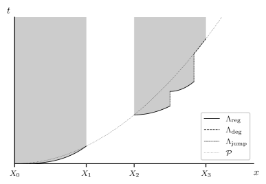
Figure 1. Sketch of the three boundary components referred to in this paper; we set $\Lambda_{\operatorname{normal}}=\Lambda_{\operatorname{reg}}\cup\Lambda_{\operatorname{deg}}$.

To proceed, set

$$\Lambda_{\operatorname{normal}}=\Lambda_{\operatorname{reg}}\cup\Lambda_{\operatorname{deg}}$$ (3.6)

and let $I$ denote the closed union of the $x$-projection of the precipitation rings, i.e.,

$$I=\bigcup_{i}\,[X_{2i},X_{2i+1}]\,.$$ (3.7)

By construction, whenever $x\in I$, there exists a unique $t\geq 0$ such that either $(x,t)\in\Lambda_{\operatorname{reg}}$ or $(x,t)\in\Lambda_{\operatorname{deg}}$. Hence, we can parametrize onset of precipitation in time with a function $\ell\colon I\to\mathbb{R}_{+}$, the precipitation front, satisfying

$$\Lambda_{\operatorname{normal}}=\{(x,\ell(x))\colon x\in I\}\,.$$ (3.8)

Lemma 13.

Let $(u,p)$ be a weak solution to (1.1) with ring domain ${\operatorname{RD}}$. Then

1. When $x\in I$, $u(x,\ell(x))=u^{*}$ and $u(x,t)<u^{*}$ for all $t\in[0,\ell(x))$.

2. $\ell$ is strictly increasing and left-continuous on $I$,

3. $\ell$ is right-continuous at every $X_{2j}$ with $\ell(X_{2j})=(X_{2j}/\alpha)^{2}$.

Proof.

For $(x,\ell(x))\in\Lambda_{\operatorname{reg}}$, statement (i) holds by definition of $\Lambda_{\operatorname{reg}}\subset C$.

If $(x,\ell(x))\in\Lambda_{\operatorname{deg}}$, we argue by contradiction. First, suppose $u(x,\ell(x))<u^{*}$. Then there exists a neighborhood of $\{x\}\times[0,x^{2}/\alpha^{2}]$ on which $u<u^{*}$ which carves out a part of $\mathcal{P}$ that contains $(x,\ell(x))$. Thus, $x$ is not contained in a ring, contradicting the definition of $\Lambda_{\operatorname{deg}}$. Else, if $u(x,\ell(x))>u^{*}$, there exists a neighborhood of $(x,\ell(x))$ on which $u>u^{*}$. Thus, by continuity, there exists $t<\ell(x)$ such that $(x,t)\in\Lambda_{\operatorname{reg}}$, again contradicting the definition of $\Lambda_{\operatorname{deg}}$.

For (ii), we first note that the argument used in the proof of Lemma 11 applies literally and proves that $\ell$ is strictly increasing. Further, it is bounded, so possesses a right limit at every point that is not a left boundary point. Taking $x\in I$ with $x\neq X_{2j}$ and setting $\ell^{*}=\lim_{y\nearrow x}\ell(y)$, we have, by continuity of $u$,

$$u(x,\ell^{*})=\lim_{y\nearrow x}u(y,\ell(y))=u^{*}\,.$$ (3.9)

This shows that $(x,\ell^{*})\notin S$ so that, due to the ordering (3.3), we have $\ell^{*}\geq\ell(x)$. On the other hand, as $\ell$ is increasing, $\ell^{*}\leq\ell(x)$. This proves that $\ell^{*}=\ell(x)$, i.e., $\ell$ is left-continuous on $I$.

To prove (iii), note that $0\leq\ell(x)\leq x^{2}/\alpha^{2}$ for $x\in I$, so $\ell(0)=0$. For $j>0$, suppose that $\ell(X_{2j})<(X_{2j}/\alpha)^{2}$. Then, due to Lemma 6, the precipitation condition (1.4) is satisfied for $x\in(\alpha\sqrt{\ell(X_{2j})},X_{2j})$, i.e.

$$\max_{s\in[0,\ell(X_{2j})]}u(x,s)>u(X_{2j},\ell(X_{2j}))=u^{*}\,.$$ (3.10)

Thus, the $j$th ring must start no farther than $x=\alpha\sqrt{\ell(X_{2j})}$, contradiction. Thus, $\ell(X_{2j})=(X_{2j}/\alpha)^{2}$ and, since $\ell$ is increasing, $\ell(X_{2j})\leq\ell(x)\leq x^{2}/\alpha^{2}$ for $x\geq X_{2j}$. Thus $\ell$ is right-continuous at this point. ∎

Lemma 14.

Let $(u,p)$ be a weak solution to (1.1) with ring domain ${\operatorname{RD}}$. On ${\operatorname{RD}}$, $p$ can be identified, up to modification on sets of measure zero, with

$$p(x,t)=\begin{cases}\mathbb{I}_{\{t>\ell(x)\}}(x,t)&\text{if $x\in I$}\\ 0&\text{otherwise}\,.\end{cases}$$ (3.11)

Proof.

On $D_{o}\cap{\operatorname{RD}}$, the value of $p$ is determined a.e. by the definition of ring domain as a sequence of rings and interrings and agrees with (3.11). On $P$ and $S$, $p$ takes values $1$ and $0$, respectively. Due to the ordering (3.3) and the definition of $\ell$, these values also agree with (3.11). This already suffices, because, by Lemma 11, the three sets $D_{o}\cap{\operatorname{RD}}$, $P$, and $S$ cover the ring domain up to sets of measure zero (those being $C$, $\mathcal{P}$, and the line $\{x=0\}$). ∎

Corollary 15.

In the setting of Lemma 14, let $(x,t)\in{\operatorname{RD}}\setminus\Lambda_{\operatorname{normal}}$. Then there exists a rectangular neighborhood $B=(x_{1},x_{2})\times(t_{1},t_{2})\subset{\operatorname{RD}}\setminus\Lambda_{\operatorname{normal}}$ of $(x,t)$ such that $p(y,s)=p^{*}(y)$ for all $(y,s)\in B$.

Proof.

$\Lambda_{\operatorname{normal}}$ is closed, so ${\operatorname{RD}}\setminus\Lambda_{\operatorname{normal}}$ is open. Since, by (3.11) and Lemma 13, for fixed $y$, $p(y,s)$ changes value only if $(y,s)\in\Lambda_{\operatorname{normal}}$, the claim is obvious. ∎

4. On the differentiability of $u$ and the continuity of $u_{t}$

In this section, we provide conditions on the existence of a classical time derivative for the solution to the HHMO-model. It turns out that $u-\psi$ is always time-differentiable away from the location of onset of precipitation. However, time-differentiability may fail on the precipitation boundary $\Lambda_{\operatorname{normal}}$. In Theorem 16, we show that time-differentiability is equivalent to continuity of the formal time derivative. Afterwards, in Lemma 17, we present a sufficient condition: essentially, time-differentiability holds at points where the precipitation front is transversal to time levels $t=\text{const}$.

Theorem 16.

Let $(u,p)$ be a weak solution to (1.1) with ring domain ${\operatorname{RD}}$. Set

$$\mathcal{F}_{1}(x,t)=\int_{0}^{t}\,\int_{\mathbb{R}}\Phi(x-y,t-s)\,p(y,s)\,u_{t}(y,s)\,\mathrm{d}y\,\mathrm{d}s\,,$$ (4.1a)

$$\mathcal{F}_{2}(x,t)=\int_{I(u)}\Phi(x-y,t-\ell(y))\,\mathrm{d}y\,.$$ (4.1b)

Then $u-\psi$ is differentiable in time near $(x,t)\in{\operatorname{RD}}$ and $(u-\psi)_{t}$ is continuous at $(x,t)$ if and only if $\mathcal{F}_{2}$ is continuous at $(x,t)$. At a point of continuity,

$$(u-\psi)_{t}=-\mathcal{F}_{1}-u^{*}\,\mathcal{F}_{2}\,.$$ (4.2)

The set of points of continuity includes ${\operatorname{RD}}\setminus\Lambda_{\operatorname{normal}}$.

Remark 4.

In the definition of $\mathcal{F}_{2}$, we use the convention that $\Phi(x-y,t-\ell(y))=0$ for $t<\ell(y)$. In the proof, we show that $\mathcal{F}_{1}$ and $\mathcal{F}_{2}$ are well-defined even though we cannot exclude that there are points $(x,t)\in\Lambda_{\operatorname{normal}}$ where $\mathcal{F}_{1}(x,t)=-\infty$ or $\mathcal{F}_{2}(x,t)=\infty$.

Remark 5.

The difficulty with showing that $\mathcal{F}_{2}$ is continuous is seen as follows. Suppose $\ell(y)=t-(x-y)^{2}$ near $y=x$. Then $\Phi(x-y,t-\ell(y))=\text{const}\cdot\lvert x-y\rvert^{-1}$, which is not integrable. Thus, continuity of $\mathcal{F}_{2}$ at a boundary point necessarily depends on the geometry of the precipitation front. For example, if the front advances at a non-vanishing rate, $\Phi(x-y,t-\ell(y))$ remains integrable and continuity of $\mathcal{F}_{2}$ follows, e.g., by approximating the integrand by a sequence of continuous compactly supported functions. We discuss sufficient conditions for continuity in Lemma 17 and Lemma 19 further below.

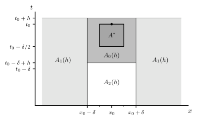
Figure 2. Sketch of splitting of the domain of integration in the proof of Theorem 16.

Proof.

We begin by introducing useful notation. For any function of two variables, $f(x,t)$, and any $h\neq 0$, we write

$$\Delta_{h}f(x,t)=\frac{f(x,t+h)-f(x,t)}{h}\,.$$ (4.3)

For any fixed $(x_{0},t_{0})\in{\operatorname{RD}}\setminus\Lambda_{\operatorname{normal}}$ and $\delta>0$, we introduce the subdomains

$$A_{0}(h)=(x_{0}-\delta,x_{0}+\delta)\times(t_{0}-\delta+h,t_{0}+h)\,,$$ (4.4a)

$$A_{1}(h)=\mathbb{R}\setminus(x_{0}-\delta,x_{0}+\delta)\times(0,t_{0}+h)\,,$$ (4.4b)

$$A_{2}(h)=(x_{0}-\delta,x_{0}+\delta)\times(0,t_{0}-\delta+h]\,,$$ (4.4c)

and

$$A^{*}=(x_{0}-\delta/2,x_{0}+\delta/2)\times(t_{0}-\delta/2,t_{0})\,;$$ (4.4d)

see Figure 2. Due to Corollary 15, we can choose $\delta$ sufficiently small such that for a.e. $y\in(x_{0}-\delta,x_{0}+\delta)$,

$$p(y,s)=p^{*}(y)$$ (4.5)

for all $s\in(t_{0}-\tfrac{5}{4}\delta,t_{0}+\frac{1}{4}\delta)$. We also choose $\delta$ sufficiently small that this time interval lies within the temporal extent of the ring domain ${\operatorname{RD}}$. Then for all $\lvert h\rvert<\delta/4$, which we assume henceforth, we can use (4.5) in any integral over the subregion $A_{0}(h)$. The proof now proceeds in five distinct steps.

Step 1.

There exists a finite constant $C>0$ which may depend on the choice of $(x_{0},t_{0})\in{\operatorname{RD}}\setminus\Lambda_{\operatorname{normal}}$ and $\delta$ such that

$$\sup_{\begin{subarray}{c}(x,t)\in A^{*}\\ \lvert h\rvert<\delta/4\end{subarray}}\,\lvert\Delta_{h}u(x,t)\rvert<C\,.$$ (4.6)

Proof of Step 1.

First, we note that $\psi(x,t)$ is absolutely continuous in $t$ with a uniform bound $C^{*}$ on $\psi_{t}$ where it exists and for $t$ bounded away from zero. Therefore, Lemma 8 implies that for every $(x,t)\in{\operatorname{RD}}$ and $h$ small enough,

$$\Delta_{h}u(x,t)\leq\Delta_{h}\psi(x,t)\leq C^{*}\,.$$ (4.7)

Thus, the main task is to find a lower bound for $\Delta_{h}u$.

A weak solution to the HHMO-model satisfies the Duhamel formula

$$u(x,t)=\psi(x,t)-\int_{0}^{t}\int_{\mathbb{R}}\Phi(x-y,t-s)\,p(y,s)\,u(y,s)\,\mathrm{d}y\,\mathrm{d}s\,,$$ (4.8)

see, e.g., [5] for a detailed discussion of the functional setting. Fix $(x,t)\in A^{*}$. Using (4.8) for each of the two terms in the finite difference $\Delta_{h}u(x,t)$, breaking up the domain of integration into $A_{0}(h)$, $A_{1}(h)$, and $A_{2}(h)$ for the first term and $A_{0}(0)$, $A_{1}(0)$, and $A_{2}(0)$ for the second, separating out the difference between these sets of integration, performing a “summation by parts” by change of variables on the subdomain $A_{0}(0)$, and using (4.5) on the part of the domain where it is applicable, we find that

$$\Delta_{h}u(x,t) =\Delta_{h}\psi(x,t)-\iint_{A_{0}(0)}\Phi(x-y,t-s)\,p^{*}(y)\,\Delta_{h}u(y,s)\,\mathrm{d}y\,\mathrm{d}s$$

$$\quad-\iint_{A_{1}(\max(0,h))}\Delta_{h}\Phi(x-y,t-s)\,p(y,s)\,u(y,s)\,\mathrm{d}y\,\mathrm{d}s$$

$$\quad-\iint_{A_{2}(\min(0,h))}\Delta_{h}\Phi(x-y,t-s)\,p(y,s)\,u(y,s)\,\mathrm{d}y\,\mathrm{d}s$$

$$\quad-\frac{1}{h}\iint_{A_{2}(0)\bigtriangleup A_{2}(h)}\Phi(x-y,t-s+\max(0,h))\,p^{*}(y)\,u(y,s)\,\mathrm{d}y\,\mathrm{d}s$$

$$\equiv\Delta_{h}\psi(x,t)+\mathcal{I}_{0}+\mathcal{I}_{1}+\mathcal{I}_{2}+\mathcal{I}_{2}^{*}\,,$$ (4.9)

where $A\bigtriangleup B=(A\setminus B)\cup(B\setminus A)$ denotes the symmetric difference of the sets $A$ and $B$. We remark that we only need to account for the symmetric difference between the sets $A_{2}(0)$ and $A_{2}(h)$; the other symmetric differences are implicit via the convention that $\Phi(x-y,t-s)=0$ for $s>t$.

The first term on the right of (4.9) is bounded below by uniform absolute continuity of $\psi$ as before. Next, due to (4.7),

$$\mathcal{I}_{0}\geq-C^{*}\int_{0}^{t_{0}}\int_{\mathbb{R}}\Phi(x-y,t-s)\,\mathrm{d}y\,\mathrm{d}s=-C^{*}\,t_{0}\,.$$ (4.10)

To proceed, recall that $u\leq\Psi(\alpha)$ by Lemma 7 and note that the effective horizontal domain of integration is bounded. Moreover,

$$\sup_{\begin{subarray}{c}(y,s)\in A_{1}(\max(0,h))\\ (x,t)\in A^{*}\end{subarray}}\,\Delta_{h}\Phi(x-y,t-s)\leq\sup_{\begin{subarray}{c}\lvert y\rvert\geq\delta/4\\ t\geq\delta/4\end{subarray}}\,\Phi_{t}(y,s)$$ (4.11)

is bounded. This provides the lower bound for $\mathcal{I}_{1}$; an analogous argument is made for $\mathcal{I}_{2}$.

Finally, we note that $m(A_{2}(0)\bigtriangleup A_{2}(h))=2\delta h$. Moreover, as in (4.11), the singularity of the heat kernel is at least a distance $\delta/4$ away from the domain of integration whenever $(x,t)\in A^{*}$. Thus, $\mathcal{I}_{2}^{*}$ is also bounded below. This concludes the proof of Step 1. ∎

Step 2.

The function $u-\psi$ is time-differentiable at $(x_{0},t_{0})\in{\operatorname{RD}}\setminus\Lambda_{\operatorname{normal}}$ with

$$(u-\psi)_{t}(x_{0},t_{0}) =-\int_{x_{0}-\delta}^{x_{0}+\delta}\int_{t_{0}-\delta}^{t_{0}}\Phi(x_{0}-y,t_{0}-s)\,u_{t}(y,s)\,\mathrm{d}s\,p^{*}(y)\,\mathrm{d}y$$

$$\quad-\iint_{A_{0}(0)^{c}}\Phi_{t}(x_{0}-y,t_{0}-s)\,p(y,s)\,u(y,s)\,\mathrm{d}y\,\mathrm{d}s$$

$$\quad-\int_{x_{0}-\delta}^{x_{0}+\delta}\Phi(x_{0}-y,\delta)\,p^{*}(y)\,u(y,t_{0}-\delta)\,\mathrm{d}y$$ (4.12)

for some $\delta>0$.

Proof of Step 2.

We employ the domain partition (4.4) with $\delta$ reduced to half its value from Step 1. Formula (4.9) remains valid on this new partition. We fix $(x,t)=(x_{0},t_{0})$ and pass to the limit $h\to 0$ in each of the terms on its right hand side as follows.

On $A_{0}$, Step 1 implies that for every fixed $y\in(x_{0}-\delta,x_{0}+\delta)$, $u(y,s)$ is absolutely continuous as a function of $s$ on the interval $(t_{0}-\delta,t_{0})$ and therefore differentiable a.e. in time with $\lvert u_{t}\rvert\leq C$. Hence, by the dominated convergence theorem,

$$\lim_{h\to 0}\int_{t_{0}-\delta}^{t_{0}}\Phi(x_{0}-y,t_{0}-s)\,\Delta_{h}u(y,s)\,\mathrm{d}s=\int_{t_{0}-\delta}^{t_{0}}\Phi(x_{0}-y,t_{0}-s)\,u_{t}(y,s)\,\mathrm{d}s\,.$$ (4.13)

A second application of the dominated convergence theorem, using

$$y\mapsto C\int_{t_{0}-\delta}^{t_{0}}\Phi(x_{0}-y,t_{0}-s)\,\mathrm{d}s$$ (4.14)

as the dominating function, then establishes that $\mathcal{I}_{0}$ converges to the first term on the right of (4.12).

For the remaining terms, due to the boundedness of $u$, $\Phi$, and $\Phi_{t}$, we invoke the dominated convergence theorem directly to establish convergence to the corresponding terms on the right of (4.12). ∎

Remark 6.

In the proof of Step 2, Borel-measurability of $u_{t}$ on $A_{0}$ is not easily asserted so that we claim the first term on the right of (4.12) only in the sense of iterated partial integrals. However, once (4.12) is established, measurability in two dimensions is obvious a posteriori; see Step 3 below.

Step 3.

$(u-\psi)_{t}$ satisfies (4.2) on ${\operatorname{RD}}\setminus\Lambda_{\operatorname{normal}}$.

Proof of Step 3.

Step 2 shows that $u-\psi$ is time-differentiable on ${\operatorname{RD}}\setminus\Lambda_{\operatorname{normal}}$. In particular, $u_{t}$ exists a.e. on ${\operatorname{RD}}$ and is measurable as the pointwise limit of the measurable function $\Delta_{h}u$. We can thus revisit the limit of $\mathcal{I}_{0}$, applying the dominated convergence theorem directly on the subdomain $A_{0}(0)$. This proves that

$$\lim_{h\to 0}\mathcal{I}_{0}=\iint_{A_{0}(0)}\Phi(x_{0}-y,t_{0}-s)\,p^{*}(y)\,u_{t}(y,s)\,\mathrm{d}s\,\mathrm{d}y\,.$$ (4.15)

To rewrite the remaining terms in (4.12), we note once again that $u_{t}$ is measurable and consider the integral

$$\mathcal{I}_{0}^{*}=\iint_{A_{0}(0)^{c}}\Phi(x_{0}-y,t_{0}-s)\,p(y,s)\,u_{t}(y,s)\,\mathrm{d}y\,\mathrm{d}s\,.$$ (4.16)

By Corollary 9 and 10, the integrand in this expression has an integrable upper bound. Thus, we can apply the Fubini theorem to the positive part of the integrand and the Tonelli theorem to the negative part, to write

$$\mathcal{I}_{0}^{*}=\int_{I^{*}}\int_{\ell(y)}^{c(y)}\Phi(x_{0}-y,t_{0}-s)\,u_{t}(y,s)\,\mathrm{d}s\,\mathrm{d}y\,,$$ (4.17)

where $c(y)=t_{0}-\delta$ for $y\in(x_{0}-\delta,x_{0}+\delta)$ and $c(y)=t_{0}$ otherwise, and

$$I^{*}=\{x\in I\colon\ell(x)<c(x)\}\,.$$ (4.18)

Then, for $y\in I^{*}$, we have

$$\int_{\ell(y)}^{c(y)} \bigl{(}\Phi(x_{0}-y,t_{0}-s)\,u_{t}(y,s)-\Phi_{t}(x_{0}-y,t_{0}-s)\,u(y,s)\bigr{)}\,\mathrm{d}s$$

$$=\int_{\ell(y)}^{c(y)}\frac{\partial}{\partial s}\bigl{(}\Phi(x_{0}-y,t_{0}-s)\,u(y,s)\bigr{)}\,\mathrm{d}s$$

$$=\Phi(x_{0}-y,t_{0}-c(y))\,u(y,c(y))-\Phi(x_{0}-y,t_{0}-\ell(y))\,u(y,\ell(y))\,.$$ (4.19)

Noting that $u(y,\ell(y))=u^{*}$ and $\Phi(x_{0}-y,t_{0}-c(y))=0$ outside of $y\in(x_{0}-\delta,x_{0}+\delta)$, then combining (4.12), (4.17), and (4.19), we find that the expression from Step 2 implies (4.2). ∎

Step 4.

Suppose that $\mathcal{F}_{2}$ is continuous at $(x_{0},t_{0})\in{\operatorname{RD}}$. Then there exists a neighborhood $V$ of $(x_{0},t_{0})$ such that $u-\psi$ is differentiable in time on $V$, $(u-\psi)_{t}$ is continuous at $(x_{0},t_{0})$, and (4.2) holds at this point.

Proof of Step 4.

By continuity of $\mathcal{F}_{2}$, there exists an open neighborhood $V\subset{\operatorname{RD}}$, of $(x_{0},t_{0})$, bounded away from $t=0$, such that $\mathcal{F}_{2}$ is uniformly bounded on $V$. First, we show that $u_{t}$ is essentially bounded on $V$. Indeed, an upper bound is already given by Corollary 9.

To obtain a lower bound, notice that, by Step 3 and Lemma 8,

$$u_{t} =\psi_{t}-\mathcal{F}_{1}-u^{*}\,\mathcal{F}_{2}$$

$$\geq\psi_{t}-\int_{0}^{t}\int_{\mathbb{R}}\Phi(x-y,t-s)\,p(y,s)\,\psi_{t}(y,s)\,\mathrm{d}y\,\mathrm{d}s-u^{*}\,\sup_{(y,s)\in V}\mathcal{F}_{2}(y,s)$$ (4.20)

a.e. on $V$. The first term on the right is clearly finite on $V$, the second by Corollary 10, and the last term is finite by construction.

Second, we show that there exists $\delta>0$ such that $p\,\lvert u_{t}\rvert$ is integrable on $A=I\times(0,t_{0}+\delta)$. To see this, fix $\delta>0$ such that there exists $(x,t)\in V\setminus\Lambda_{\operatorname{normal}}$ with $t>t_{0}+\delta$ such that $(u-\psi)_{t}\leq 0$ exists at this point. Let $\sigma_{-}=-\min\{pu_{t},0\}$ and $\sigma_{+}=\max\{pu_{t},0\}$ denote the negative and positive parts of $pu_{t}$, respectively. By (2.24), $\sigma_{+}$ is essentially bounded. For $\sigma_{-}$, we estimate

$$\inf_{(y,s)\in A}\, \Phi(x-y,t-s)\iint_{A}\sigma_{-}(y,s)\,\mathrm{d}y\,\mathrm{d}s$$

$$\leq\int_{0}^{t}\int_{\mathbb{R}}\Phi(x-y,t-s)\,\sigma_{-}(y,s)\,\mathrm{d}y\,\mathrm{d}s$$

$$=(u-\psi)_{t}+\mathcal{F}_{1}^{+}+u^{*}\,\mathcal{F}_{2}\,,$$ (4.21)

where

$$\mathcal{F}_{1}^{+}=\int_{0}^{t}\int_{\mathbb{R}}\Phi(x-y,t-s)\,\sigma_{+}(y,s)\,\mathrm{d}y\,\mathrm{d}s$$ (4.22)

is bounded due to Corollary 9 and 10. Since $\Phi(x-y,t-s)$ has a positive lower bound on $A$ and all terms on the right hand side of (4.21) are bounded, $\sigma_{-}$ is integrable on $A$, and so is $p\,\lvert u_{t}\rvert$.

Now, for every $(x,t)\in A$,

$$\mathcal{F}_{1}(x,t) =\iint_{A\setminus V}\Phi(x-y,t-s)\,p(y,s)\,u_{t}(y,s)\,\mathrm{d}y\,\mathrm{d}s$$

$$\quad+\iint_{A\cap V}\Phi(x-y,t-s)\,p(y,s)\,u_{t}(y,s)\,\mathrm{d}y\,\mathrm{d}s\,.$$ (4.23)

The first term is continuous by the dominated convergence theorem as $p\,\lvert u_{t}\rvert$ is integrable and the kernel is bounded on $A\setminus V$ uniformly for $(x,t)$ near $(x_{0},t_{0})$. The second term is bounded as a convolution of an $L^{1}$ with an $L^{\infty}$ function as $u_{t}$ is bounded on $V$.

When $(x_{0},t_{0})\in{\operatorname{RD}}\setminus\Lambda_{\operatorname{normal}}$, the claim follows directly from formula (4.2) proved in Step 3. When $(x_{0},t_{0})\in{\operatorname{RD}}\cap\Lambda_{\operatorname{normal}}$, we note that (4.2) holds for $x=x_{0}$ fixed and a.e. $t$ near $t_{0}$ and the right hand side of (4.2) is continuous at $(x_{0},t_{0})$. Hence, we can use (4.2) to continuously extend $(u-\psi)_{t}$ to the point $(x_{0},t_{0})$. ∎

Step 5.

Suppose that there exists an open neighborhood $V$ of $(x_{0},t_{0})\in{\operatorname{RD}}$ such that $u-\psi$ is differentiable in time on $V$ and $(u-\psi)_{t}$ is continuous at $(x_{0},t_{0})$. Then $\mathcal{F}_{2}$ is continuous at $(x_{0},t_{0})$ and (4.2) holds at this point.

Proof of Step 5.

Since $(u-\psi)_{t}$ is continuous at $(x_{0},t_{0})$, $u_{t}$ exists a.e. and is essentially bounded on a possibly smaller neighborhood, again denoted $V$. Following the proof of Step 4 starting from the second claim we find, as before, that $\mathcal{F}_{1}$ is continuous at $(x_{0},t_{0})$. Turning to $\mathcal{F}_{2}$, we first show that $\mathcal{F}_{2}$ is well-defined on $V$. Indeed, on $V\setminus\Lambda_{\operatorname{normal}}$, the integrand is bounded, so $\mathcal{F}_{2}$ is finite. Now take $(x,t)\in V\cap\Lambda_{\operatorname{normal}}$. Since $\ell$ is strictly increasing, $(x+\varepsilon,t)\notin\Lambda_{\operatorname{normal}}$ for every $\varepsilon>0$ and (4.2) holds true at every such point. Moreover, $\ell(y)>t$ for $y>x$, so that $\Phi(x-y,t-\ell(y))$ can only be nonzero if $y<x$ so that, for fixed $y$, $\Phi(x+\varepsilon-y,t-\ell(y))$ is a decreasing function of $\varepsilon$. Consequently, by the monotone convergence theorem,

$$\lim_{\varepsilon\searrow 0}\mathcal{F}_{2}(x+\varepsilon,t)=\mathcal{F}_{2}(x,t)$$ (4.24)

either as a finite limit or diverging to $+\infty$. Further, taking $\limsup_{\varepsilon\searrow 0}$ of (4.2),

$$\limsup_{\varepsilon\searrow 0}(u-\Psi)_{t}(x+\varepsilon,t)=-\mathcal{F}_{1}(x,t)-u_{*}\,\mathcal{F}_{2}(x,t)\,.$$ (4.25)

Since the first two terms are finite, so is $\mathcal{F}_{2}(x,t)$. Finally, at the point $(x_{0},t_{0})$,

$$\limsup_{x\to x_{0}}\limsup_{\varepsilon\searrow 0}\,(u-\psi)_{t}(x+\varepsilon,t) =\liminf_{x\to x_{0}}\,\limsup_{\varepsilon\searrow 0}(u-\psi)_{t}(x+\varepsilon,t)$$

$$=(u-\psi)_{t}(x_{0},t_{0})\,.$$ (4.26)

Using continuity of $\mathcal{F}_{1}$ once again, we conclude that $\mathcal{F}_{2}$ is continuous at $(x_{0},t_{0})$. ∎

Since $\mathcal{F}_{2}$ is clearly continuous for every $(x,t)\notin\Lambda_{\operatorname{normal}}$ by dominated convergence, these five steps conclude the proof of Theorem 16. On $\Lambda_{\operatorname{normal}}$, the following lemma provides a sufficient condition for continuity.

Lemma 17.

Let $(u,p)$ be a weak solution to (1.1) with ring domain ${\operatorname{RD}}$. Suppose that $(x_{0},t_{0})\in\Lambda_{{\operatorname{normal}}}\cap{\operatorname{RD}}$. Then $\mathcal{F}_{2}$, defined in Theorem 16, is continuous near $(x_{0},t_{0})$ provided

$$u_{x+}(x_{0},t_{0})=\lim_{h\searrow 0}\frac{u(x_{0}+h,t_{0})-u(x_{0},t_{0})}{h}<0\,.$$ (4.27)

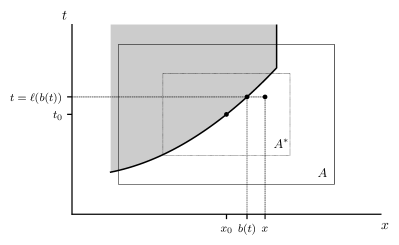
Figure 3. Sketch of the geometry of the construction used in the proof of Lemma 17.

Proof.

Since $u-\psi\in C^{1,0}({\operatorname{RD}})$, there exists a rectangular neighborhood $A$ of $(x_{0},t_{0})$ such that $u_{x+}<\frac{1}{2}\,u_{x+}(x_{0},t_{0})<0$ on $A\setminus D_{o}$. We choose $A$ small enough so that it is contained in the first quadrant, is bounded away from the $x$-axis, and intersects only one ring. Let $A^{*}$ denote a smaller neighborhood of $(x_{0},t_{0})$, strictly nested inside of $A$ (see Figure 3).

Writing

$$I_{A}=\{x\in I\colon(x,t)\in A\text{ for some }t\}\,,$$ (4.28)

we split the domain of integration in the definition of $\mathcal{F}_{2}$ into

$$\mathcal{F}_{2}(x,t)=\int_{I\setminus I_{A}}\Phi(x-y,t-\ell(y))\,\mathrm{d}y+\int_{I_{A}}\Phi(x-y,t-\ell(y))\,\mathrm{d}y\,.$$ (4.29)

The first term is continuous on $A^{*}$ by dominated convergence because the singularity of the kernel is bounded by a uniform distance away from the domain of integration. Thus, the main task is to prove that the second term is continuous on $A^{*}$ as well.

We employ the Vitali convergence theorem (e.g. [9]). First, we show that

$$\Phi(x-\,\cdot\,,t-\ell(\,\cdot\,))\to\Phi(x_{0}-\,\cdot\,,t_{0}-\ell(\,\cdot\,))$$ (4.30)

in measure as $(x,t)\to(x_{0},t_{0})$. Indeed, let $\varepsilon>0$. For every $r>0$, take an arbitrary $y$ with $\lvert x_{0}-y\rvert>r$. Then

$$\lvert\Phi(x_{0} -y,t_{0}-\ell(y))-\Phi(x-y,t-\ell(y))\rvert$$

$$\leq\lvert\Phi(x_{0}-y,t_{0}-\ell(y))-\Phi(x_{0}-y,t-\ell(y))\rvert$$

$$\quad+\lvert\Phi(x_{0}-y,t-\ell(y))-\Phi(x-y,t-\ell(y))\rvert$$

$$\leq\sup_{y\notin B(x_{0},r)}\sup_{\tau\in[t_{0}-\ell(y),t-\ell(y)]}\,\lvert\Phi_{t}(x_{0}-y,\tau)\rvert\,\lvert t_{0}-t\rvert$$

$$\quad+\sup_{y\notin B(x_{0},r)}\sup_{\xi\in[x_{0}-y,x-y]}\sup_{s\in[0,\ell(y)]}\,\lvert\Phi_{x}(\xi,s)\rvert\,\lvert x-x_{0}\rvert\,.$$ (4.31)

The suprema on the right hand side are both finite (but may depend on $r$). Therefore, it is possible to choose $\delta>0$ small enough so that the right hand side of (4.31) is less than $\varepsilon$ whenever $\lvert t_{0}-t\rvert<\delta$ and $\lvert x-x_{0}\rvert<\delta$. Thus,

$$m\{y\in\mathbb{R}\colon\lvert\Phi(x_{0}-y,t_{0}-\ell(y))-\Phi(x-y,t-\ell(y))\rvert\geq\varepsilon\}<2r\,.$$ (4.32)

Since $r$ was arbitrary, this proves that

$$\lim_{(x,t)\to(x_{0},t_{0})}m\{y\in\mathbb{R}\colon\lvert\Phi(x_{0}-y,t_{0}-\ell(y))-\Phi(x-y,t-\ell(y))\rvert\geq\varepsilon\}=0\,,$$ (4.33)

i.e., convergence in measure.

Second, we show that $\Phi(x-\,\cdot\,,t-\ell(\,\cdot\,))$ is uniformly integrable for $(x,t)\in A^{*}$. Here, it suffices to bound the integrand by a translate of a fixed integrable profile. Recalling that, by Lemma 13, $u(y,\ell(y))=u^{*}$ for all $y\in I$ and $\ell$ is strictly increasing, we find that, for $y_{1},y_{2}\in I_{A}$ with $y_{1}<y_{2}$,

$$0 =u(y_{2},\ell(y_{2}))-u(y_{1},\ell(y_{1}))$$

$$=u(y_{2},\ell(y_{2}))-u(y_{2},\ell(y_{1}))+u(y_{2},\ell(y_{1}))-u(y_{1},\ell(y_{1}))$$

$$\leq\psi(y_{2},\ell(y_{2}))-\psi(y_{2},\ell(y_{1}))+u_{x}(\xi,\ell(y_{1}))\,(y_{2}-y_{1})$$

$$=\psi_{t}(y_{2},\tau)\,(\ell(y_{2})-\ell(y_{1}))+u_{x}(\xi,\ell(y_{1}))\,(y_{2}-y_{1})\,.$$ (4.34)

The inequality in the third line is due to Lemma 8 which states that $u-\psi$ is non-increasing in time. Further, we used the mean value theorem twice, for some $\xi\in(y_{1},y_{2})$ and $\tau\in(\ell(y_{1}),\ell(y_{2}))$. We conclude that

$$\frac{\ell(y_{2})-\ell(y_{1})}{y_{2}-y_{1}}\geq-\frac{u_{x}(x_{0},t_{0})}{2\,\sup_{A}\psi_{t}}\equiv C_{A}>0\,.$$ (4.35)

In the following, take any $(x_{0},t_{0})\in A^{*}\cap\Lambda_{\operatorname{normal}}$, fix $(x,t)\in A^{*}$, and suppose that the ring intersecting $A$ intersects time-level $t$ within the interior of $A$. (If not, $\Phi(x-\,\cdot\,,t-\ell(\,\cdot\,))$ is essentially zero on $I_{A}$ and there is nothing to do.) Then for all $y,y_{2}\in I_{A}$ with $y<y_{2}$ such that $\ell(y_{2})\leq t$ we have, by (4.35),

$$t-\ell(y)\geq\ell(y_{2})-\ell(y)\geq C_{A}\,(y_{2}-y)$$ (4.36)

so that

$$t-\ell(y)\geq C_{A}\,(b(t)-y)$$ (4.37)

where $b(t)=\sup\{y\in I_{A}\colon\ell(y)\leq t\}$, see Figure 3. Hence,

$$\Phi(x-y,t-\ell(y))\leq\mathbb{I}_{y\leq b(t)}\,\frac{1}{\sqrt{4\pi\,C_{A}\,(b(t)-y)}}\,,$$ (4.38)

which, as a translate of a fixed profile, is uniformly integrable on $I_{A}$.

Finally, we note that the interval of integration is bounded, so that that the family $\Phi(x-\,\cdot\,,t-\ell(\,\cdot\,))$ restricted to $I_{A}$ is trivially tight. We conclude that the Vitali convergence theorem applies and proves that the second integral in (4.29) is continuous at $(x_{0},t_{0})$ as well. ∎

Remark 7.

If we think of $\mathcal{F}_{2}$ being defined with a general function $\ell(y)$ that does not necessarily come from the HHMO-model, there are two failure modes for the continuity of $\mathcal{F}_{2}$. The first is topological: if the number of intersections of $\ell$ with horizontal lines in the $x$-$t$ plane changes, the value of $\mathcal{F}_{2}$ can jump as $t$ is varied. In our setting, this is prevented by the strict monotonicity of $\ell$. The second failure mode is analytical: if $\ell(y)$ crosses time-level $t$ at the wrong rate, then the integral may diverge. This is illustrated by the family of functions $\ell(x)=t_{0}-(x-x_{0})\,\lvert x-x_{0}\rvert^{\gamma}$. When $\gamma=1$, the integral diverges, whereas for any $\gamma\in(-1,1)$ or $\gamma>1$, the integral is finite. In our setting, divergence is prevented by the transversality condition (4.27) which, as this discussion shows, is sufficient but clearly not necessary.

5. On uniqueness of the solutions

In the following, we prove two uniqueness theorems. The first, Theorem 18, asserts unconditional uniqueness of the solution to the HHMO-model for a short but positive interval of time. The second result, Theorem 20 proves uniqueness within the ring domain of the solution and subject to some regularity of the precipitation front, which can be expressed as transversality in time of the increase of concentration at the location of the front. The proof also shows that any breakdown of uniqueness must be accompanied by topologically complex behavior of the associated precipitation fronts.

Theorem 18 (Short-time uniqueness).

Assume that $u^{*}$ is a supercritical precipitation threshold. Then there exists a time $T_{{\operatorname{unique}}}>0$ such that any two weak solutions to (1.1) are identical on $D_{{\operatorname{unique}}}=\mathbb{R}\times[0,T_{{\operatorname{unique}}}]$.

Proof.

A weak solution to (1.1) has at least one ring with a width of at least $L$, see Remark 4. Moreover, ignition of precipitation can appear only on some restricted domain, the essential domain

$${\operatorname{ES}}(t)=\{(y,s)\colon\alpha\sqrt{s}<y<\alpha^{*}\sqrt{s},0<s<t\}\,,$$ (5.1)

where $\alpha^{*}$ is defined by (2.22). The key step in this proof is to show that there exists a positive time $T_{{\operatorname{unique}}}$ such that $u_{t}>0$ on ${\operatorname{ES}}(T_{{\operatorname{unique}}})$ for any weak solution $(u,p)$. Once this is established, uniqueness up to time $T_{{\operatorname{unique}}}$ follows by standard energy estimates.

First, we establish a negative upper bound for $u_{x}$. Differentiating the Duhamel formula (4.8), we obtain

$$u_{x}(x,t) =\psi_{x}(x,t)-\int_{0}^{t}\int_{\mathbb{R}}\Phi_{x}(x-y,t-s)\,p(y,s)\,u(y,s)\,\mathrm{d}y\,\mathrm{d}s$$

$$\leq\psi_{x}(x,t)+\Psi(\alpha)\int_{0}^{t}\int_{\{\lvert y\rvert\leq\alpha^{*}\sqrt{s}\}}\lvert\Phi_{x}(x-y,t-s)\rvert\,\mathrm{d}y\,\mathrm{d}s\,.$$ (5.2)

By direct computation,

$$\psi_{x}(x,t)\leq-\frac{\alpha\beta}{2\sqrt{t}}\,\mathrm{e}^{\tfrac{\alpha^{2}-\alpha^{*2}}{4}}$$ (5.3)

on ${\operatorname{ES}}(t)$. Further, since $\Phi_{x}(x,t)\in L^{1}(\mathbb{R}\times[0,T])$ for all $T>0$, we observe that

$$\lim_{t\searrow 0}\int_{0}^{t}\int_{\mathbb{R}}|\Phi_{x}(x-y,t-s)|\,\mathrm{d}y\,\mathrm{d}s=0\,.$$ (5.4)

Thus, there exists $T_{1}>0$ such that, on ${\operatorname{ES}}(T_{1})$, every weak solution satisfies

$$u_{x}(x,t)\leq-\frac{\alpha\beta}{4\sqrt{t}}\,\mathrm{e}^{\tfrac{\alpha^{2}-\alpha^{*2}}{4}}\,.$$ (5.5)

By Lemma 17 together with Theorem 16, this implies that $(u-\psi)_{t}$ exists and is given by (4.2) on ${\operatorname{ES}}(T_{1})$.

Second, we establish a lower bound on the growth of $\ell$. We know from Lemma 13 (ii) that $\ell$ is increasing on $\mathbb{R}_{+}$. By the Lebesgue differentiation theorem for monotonic functions, $\ell$ is differentiable almost everywhere on $[0,L]$. We denote the domain of differentiability by $U$. Then, e.g. [9, p. 108],

$$\ell(y_{2})-\ell(y_{1})\geq\int_{[y_{1},y_{2}]\cap U}\ell^{\prime}(y)\,\mathrm{d}y$$ (5.6)

for all $0<y_{1}<y_{2}\leq L$. Assuming that $y\in(0,L]\cap U$ with $\ell(y)\leq T_{1}$, a computation analogous to (4) yields

$$\ell^{\prime}(y)\geq-\frac{u_{x}(y,\ell(y))}{\psi_{t}(y,\ell(y))}\,.$$ (5.7)

We also observe that, due to Lemma 7,

$$\ell(y)\geq(y/\alpha^{*})^{2}\,.$$ (5.8)

Inserting (5.5) and (2.24) into (5.7), then using (5.8) in a second step, we estimate

$$\ell^{\prime}(y) \geq\biggl{(}\frac{C_{\psi}}{\ell(y)}\biggr{)}^{-1}\frac{\alpha\beta}{4\sqrt{\ell(y)}}\,\mathrm{e}^{\tfrac{\alpha^{2}-\alpha^{*2}}{4}}=\frac{\alpha\beta}{4C_{\psi}}\,\mathrm{e}^{\tfrac{\alpha^{2}-\alpha^{*2}}{4}}\,\sqrt{\ell(y)}$$

$$\geq\frac{\alpha\beta}{4\alpha^{*}C_{\psi}}\,\mathrm{e}^{\tfrac{\alpha^{2}-\alpha^{*2}}{4}}\,y=2\,C_{\ell}\,y$$ (5.9)

with a constant $C_{\ell}$ which is independent of the weak solution $(u,p)$. Integrating (5.9) and recalling (5.6), we obtain

$$\ell(y_{2})-\ell(y_{1})\geq C_{\ell}\,(y_{2}^{2}-y_{1}^{2})\,.$$ (5.10)

Third, we obtain upper bounds on $\mathcal{F}_{1}$ and $\mathcal{F}_{2}$, hence, a lower bound on $u_{t}$. For $\mathcal{F}_{1}$, we estimate, invoking Lemma 8 and Corollary 10, that

$$\mathcal{F}_{1}(x,t) =\int_{0}^{t}\int_{\mathbb{R}}\Phi(x-y,t-s)\,p(u,s)\,u_{t}(y,s)\,\mathrm{d}y\,\mathrm{d}s$$

$$\leq\int_{0}^{t}\int_{\mathbb{R}}\Phi(x-y,t-s)\,p(y,s)\,\psi_{t}(y,s)\,\mathrm{d}y\,\mathrm{d}s$$

$$\leq\alpha^{*}\,C_{\psi}\,\sqrt{\pi}\,.$$ (5.11)

For $\mathcal{F}_{2}$, we restrict final time to $T_{2}=\min\{(L/\alpha^{*})^{2},T_{1}\}$. Clearly, $T_{2}$ is positive, independent of the weak solution $(u,p)$, and

$$\ell(L)\geq T_{2}\,.$$ (5.12)

Setting

$$a\equiv a(t)=\sup\{y\colon\ell(y)\leq t\}$$ (5.13)

so that $a(t)\leq L$ and $\ell(a(t))\leq t$ due to the left-continuity of $\ell$, see Lemma 13(ii). Using (5.10), we find that

$$t-\ell(y)\geq\ell(a(t))-\ell(y)\geq C_{\ell}\,(a^{2}-y^{2})$$ (5.14)

for all $y$ with $\ell(y)\leq t$. Thus, for all $x\in\mathbb{R}$ and $t\in[0,T_{2}]$

$$\mathcal{F}_{2}(x,t) =\int_{I}\Phi(x-y,t-\ell(y))\,\mathrm{d}y\leq\frac{1}{\sqrt{4\pi}}\int_{-a}^{a}(t-\ell(y))^{-\tfrac{1}{2}}\,\mathrm{d}y$$

$$=\frac{1}{\sqrt{\pi}}\int_{0}^{a}(t-\ell(y))^{-\tfrac{1}{2}}\,\mathrm{d}y\leq\frac{1}{\sqrt{\pi C_{\ell}}}\int_{0}^{a}(a^{2}-y^{2})^{-\tfrac{1}{2}}\,\mathrm{d}y$$

$$=\frac{1}{\sqrt{\pi C_{\ell}}}\,\sin^{-1}\Bigl{(}\frac{y}{a}\Bigr{)}\bigg{|}^{a}_{0}=\frac{1}{2}\,\sqrt{\frac{\pi}{C_{\ell}}}\,.$$ (5.15)

On ${\operatorname{ES}}(T_{2})$, we also have a lower bound on $\psi_{t}$,

$$\psi_{t}(x,t)\geq\frac{c_{\psi}}{t}$$ (5.16)

with

$$c_{\psi}=\frac{\alpha\beta}{4}\,\mathrm{e}^{\tfrac{\alpha^{2}}{4}}\,\min_{y\in[\alpha,\alpha^{*}]}y\,\mathrm{e}^{\tfrac{-y^{2}}{4}}>0\,.$$ (5.17)

Altogether, inserting the bounds (5.11), (5.15), and (5.16) into (4.2), we obtain

$$u_{t}(x,t) =\psi_{t}(x,t)-\mathcal{F}_{1}(x,t)-u^{*}\,\mathcal{F}_{2}(x,t)$$

$$\geq\frac{c_{\psi}}{t}-\alpha^{*}\,C_{\psi}\,\sqrt{\pi}-\frac{u^{*}}{2}\,\sqrt{\frac{\pi}{C_{\ell}}}\,.$$ (5.18)

We conclude that for any weak solution, $u_{t}$ is strictly positive in the interior of ${\operatorname{ES}}(T_{{\operatorname{unique}}})$, where

$$T_{{\operatorname{unique}}}=\min\biggl{\{}T_{2},c_{\psi}\Big{/}\Bigl{(}\alpha^{*}\,C_{\psi}\,\sqrt{\pi}+\frac{u^{*}}{2}\,\sqrt{\frac{\pi}{C_{\ell}}}\Bigr{)}\biggr{\}}$$ (5.19)

independent of the weak solution $(u,p)$.

Now suppose that $(u_{1},p_{1})$ and $(u_{2},p_{2})$ are weak solutions of (1.1). We claim that, on $D_{{\operatorname{unique}}}=\mathbb{R}\times[0,T_{{\operatorname{unique}}}]$,

$$(p_{1}u_{1}-p_{2}u_{2})(u_{1}-u_{2})_{+}\geq 0\,.$$ (5.20)

We prove this claim separately on three subdomains. On $D_{o}\cap D_{{\operatorname{unique}}}$, $p_{1}=p_{2}=1$ because $T_{{\operatorname{unique}}}$ is selected such that the $x$-projection of this set is included in the first ring. Hence, the claim is obvious. On $D^{*}\cap D_{{\operatorname{unique}}}$ and on its symmetric counterpart in the left half-plane, $p_{1}=p_{2}=0$ due to Lemma 7; the claim is also obvious. Finally, on ${\operatorname{ES}}(T_{{\operatorname{unique}}})$, we note that $(p_{1}u_{1}-p_{2}u_{2})(u_{1}-u_{2})_{+}$ can be negative only if $u_{1}(x,t)>u_{2}(x,t)$ and $p_{1}(x,t)<1$. By Lemma 14, we may assume that $p_{1}$ and $p_{2}$ are of the form (3.11). Therefore, $p_{1}(x,t)<1$ implies $u^{*}\geq u_{1}(x,t)$. But then $u^{*}\geq u_{1}(x,t)>u_{2}(x,t)$. Since $u_{2}$ is increasing in time on ${\operatorname{ES}}(T_{{\operatorname{unique}}})$, we have $u^{*}>u_{2}(x,s)$ if $(x,s)\in{\operatorname{ES}}(t)\subset{\operatorname{ES}}(T_{{\operatorname{unique}}})$. So precipitation cannot start at spatial coordinate $x$ until after time $t$, thus $p_{2}(x,t)=0$. Hence, $(p_{1}u_{1}-p_{2}u_{2})(u_{1}-u_{2})_{+}=p_{1}u_{1}(u_{1}-u_{2})_{+}\geq 0$ at $(x,t)\in{\operatorname{ES}}(T_{{\operatorname{unique}}})$. This proves (5.20).

We complete the proof with a direct energy estimate. Proceeding formally (a first-principles justification can be found in [5]), we note that

$$(u_{1}-u_{2})_{t}=(u_{1}-u_{2})_{xx}-p_{1}\,u_{1}+p_{2}\,u_{2}\,,$$ (5.21)

multiply with $(u_{1}-u_{2})_{+}$, integrate in space and then integrate by parts,

$$\frac{1}{2}\frac{\mathrm{d}}{\mathrm{d}t}\int_{\mathbb{R}}(u_{1}-u_{2})_{+}^{2}\,\mathrm{d}x\\ =-\int_{\mathbb{R}}\mathbb{I}_{\{u_{1}>u_{2}\}}\,(u_{1}-u_{2})_{x}^{2}\,\mathrm{d}x-\int_{\mathbb{R}}(p_{1}u_{1}-p_{2}u_{2})(u_{1}-u_{2})_{+}\,\mathrm{d}x\leq 0\,.$$ (5.22)

Integrating in time with $u_{1}(x,0)-u_{2}(x,0)=0$, we find that $u_{2}\geq u_{1}$ on $D_{{\operatorname{unique}}}$. As the argument is symmetric under exchange of indices, we also have the reverse inequality, so $u_{1}=u_{2}$ on $D_{{\operatorname{unique}}}$. An easy argument shows that the precipitation function is essentially determined by the concentration field (e.g. [8, Lemma 3]), hence $p_{1}=p_{2}$ a.e. on $D_{{\operatorname{unique}}}$. ∎

Lemma 19.

Let $(u,p)$ be a weak solution to (1.1) with ring domain ${\operatorname{RD}}$. Suppose that there exists $X\leq X^{*}$ such that

$$\limsup_{k\searrow 0}\Delta_{k}^{-}u(x,t)\equiv\limsup_{k\searrow 0}\frac{u(x,\ell(x))-u(x,\ell(x)-k)}{k}>0$$ (5.23)

for all $x\in D\equiv I(u)\cap(0,X)$. Then the one-sided derivatives $u_{x+}(x,\ell(x))$ and $u_{t-}(x,\ell(x))$ exist for all $x\in D$ with $u_{x+}(x,\ell(x))<0$ and $u_{t-}(x,\ell(x))>0$.

Remark 8.

In contrast to the local statement in Lemma 17, the transversality condition (5.23) here must be satisfied globally on the domain $I(u)\cap(0,X)$.

Remark 9.

At points $(x,\ell(x))$ on the precipitation boundary that do not lie on the parabola $\mathcal{P}$, the one-sided derivatives in Lemma 19 are regular two-sided derivatives. For $u_{x}$, this follows directly from the concept of weak solution, for $u_{t}$, this is a consequence of Lemma 17.

Remark 10.

In the proof of Theorem 18, we have already proved that classical first derivatives exist, with $u_{x}(x,\ell(x))<0$ and $u_{t}(x,\ell(x))>0$, on the part of the precipitation boundary contained in $D_{{\operatorname{unique}}}$.

Remark 11.

So long as one of the transversality conditions from Lemma 19 or Lemma 17 is satisfied, thus at least for some initial interval of time, $u$ is continuously differentiable in time away from the parabola $\mathcal{P}$. Thus, the discontinuity of the precipitation term in the HHMO-model must be balanced by a discontinuity of $u_{xx}$ across the precipitation boundary. This behavior is not obvious from a direct inspection of the PDE.

Proof.

Take $x\in(0,X^{*})$ such that for all $y\in I(u)\cap(0,x)$, the one-sided derivatives $u_{x+}(y,\ell(y))$ and $u_{t-}(y,\ell(y))$ exist with $u_{x+}(y,\ell(y))<0$ and $u_{t-}(y,\ell(y))>0$. (Such an $x$ exists, see Remark 10.) Suppose further that the transversality condition (5.23) remains satisfied at $x$. We shall show that this implies that $u_{x+}(y,\ell(y))$ and $u_{t-}(y,\ell(y))$ exist with $u_{x+}(y,\ell(y))<0$ and $u_{t-}(y,\ell(y))>0$ in a neighborhood of $x$ that is relatively open in $I(u)\cap(0,X)$. This implies the lemma as stated.

In the following, set $t=\ell(x)$. Our main the main task is to show that $u_{x+}(x,t)<0$, a claim which we prove in three distinct cases below. Once this is established, Lemma 17 implies that $(x,t)$ is a point of continuity of $(u-\psi)_{t}$; in particular, $u_{t-}(x,t)$ is defined and is positive. When $x$ is the right boundary point of a ring, this is all we have to show. Otherwise, we assert that $\ell$ is right-continuous at $x$. Indeed, when $(x,t)\in\mathcal{P}$, this is trivial. When $(x,t)\notin\mathcal{P}$, $u_{t}(x,t)$ is defined and strictly positive, so that $u(x,t+k)>u^{*}$ for every sufficiently small $k>0$, $(x,t)\notin\Lambda_{\operatorname{jump}}$, and $\ell$ is continuous at $(x,t)$. Right-continuity of $\ell$ at $x$ implies that the one-sided derivatives exist $u_{x+}(y,\ell(y))$ and $u_{t-}(y,\ell(y))$ exist with their signs preserved in a right neighborhood of $x$, which completes the argument.

Case 1.

$u_{x+}(x,t)<0$ if $(x,t)\in\mathcal{P}$ and $x$ is not the left boundary point of a ring.

Take $h>0$ small enough so that $x-h$ is contained in the same ring. As in the proof of Lemma 17,

$$u(x,t)=u^{*}=u(x-h,\ell(x-h))\,,$$ (5.24)

so that

$$\frac{\ell(x)-\ell(x-h)}{h}\cdot\frac{u(x,t)-u(x,\ell(x-h))}{\ell(x)-\ell(x-h)}=-\frac{u(x,\ell(x-h))-u(x-h,\ell(x-h))}{h}\,.$$ (5.25)

Noting that $\ell(x)=x^{2}/\alpha^{2}$ and $\ell(x-h)\leq(x-h)^{2}/\alpha^{2}$, so that $\ell(x)-\ell(x-h)\geq({2xh}-{h^{2}})/{\alpha^{2}}$, we find that for $h$ sufficiently small,

$$\frac{\ell(x)-\ell(x-h)}{h}\geq\frac{x}{\alpha^{2}}>0\,.$$ (5.26)

By Lemma 13(ii), $\ell$ is left-continuous and strictly increasing. Due to the transversality condition (5.23), this implies that

$$\limsup_{h\searrow 0}\frac{u(x,t)-u(x,\ell(x-h))}{\ell(x)-\ell(x-h)}>0\,.$$ (5.27)

Last, as $\ell$ is strictly increasing, the open line segment $\{(\xi,\ell(x-h))\colon x-h<\xi<x\}$ lies below the precipitation boundary for every such $h$. Since $u_{x}$ is continuous on this line segment, the mean value theorem yields

$$\frac{u(x-h,\ell(x-h))-u(x,\ell(x-h))}{h}=u_{x}(\xi(h),\ell(x-h))$$ (5.28)

for some $\xi(h)\in(x-h,x)$. Using left-continuity of $\ell$ and the fact that $u-\psi$ is continuously differentiable in $x$, we find

$$\lim_{h\searrow 0}\frac{u(x-h,\ell(x-h))-u(x,\ell(x-h))}{h}=u_{x+}(x,t)\,.$$ (5.29)

Thus, letting $h\searrow 0$ in (5.25) and referring to (5.26), (5.27), and (5.29) for each of the terms, we conclude that $u_{x+}(x,t)<0$.

Case 2.

$u_{x+}(x,t)<0$ if $x=X_{2i}$, i.e., $x$ is the starting location of a ring.

In this case, $(x,t)\in\mathcal{P}$ by Lemma 13(iii) and the location of the singularity of the heat kernel in the Duhamel integral is bounded away from the effective domain of integration, so that we can differentiate the Duhamel formula directly to find

$$u_{t-}(x,t)=\psi_{t-}(x,t)-\int_{0}^{t}\int_{\mathbb{R}}\Phi_{t}(x-y,t-s)\,p(y,s)\,u(y,s)\,\mathrm{d}y\,\mathrm{d}s\,.$$ (5.30)

This shows that $u_{t-}$ exists and is continuous on the ray $[x,\infty)\times\{t\}$. To proceed, we recall that $\ell$ is increasing and left-continuous, so that on any box with upper left corner $(x,t)$, $p=0$ so that $u$ solves the heat equation $u_{t}=u_{xx}$. Then, by the Taylor formula with integral remainder,

$$u(x+h,t)=u(x,t)+u_{x+}(x,t)\,h+\int_{x}^{x+h}(x+h-\xi)\,u_{t}(\xi,t)\,\mathrm{d}\xi\,.$$ (5.31)

Since $u^{*}=u(x,t)\geq u(x+h,t)$ and the integral in (5.31) is strictly positive for $h$ small enough due to continuity of $u_{t-}$ and the transversality condition (5.23), we conclude that $u_{x+}(x,t)<0$.

Case 3.

$u_{x+}(x,t)<0$ if $(x,t)\notin\mathcal{P}$.

Figure 4. Sketch of the geometry of the construction used in the proof of Lemma 19, Case 3.

This case cannot be solved by a local argument, as we have no lower bound on the growth of $\ell$ as in (5.26). We take $x_{0}<x$ large enough such that $x_{0}$ is the same ring as $x$ and $(x_{0},t)$ lies below the parabola $\mathcal{P}$. We split the space-time domain into three subregions, see Figure 4:

$$A_{1}=(-\infty,x_{0})\times(0,t)\,,$$ (5.32a)

$$A_{2}=\{(y,s)\colon x_{0}<y<x,\ell(y)<s\leq t\}\,,$$ (5.32b)

$$A_{3}=\{(y,s)\colon x_{0}<y,0<s<\min\{\ell(y),t\}\}\,.$$ (5.32c)

We now proceed in three steps. In the first step, we show that $u_{t}$ is bounded on $A_{2}$. By Lemma 8, $u_{t}$ is bounded above, so it suffices to find a lower bound. We first note that on $\Gamma_{1}$, the right boundary of $A_{1}$, $u_{t}$ is continuous up to the boundary points, hence is bounded. On $\Gamma_{2}$, the joint boundary of $A_{2}$ and $A_{3}$ we have $u_{t}>0$ by assumption except perhaps at the end point $(x,t)$ where we do not know yet whether $u_{t}$ is defined. (Recall that the continuation argument implies that $\ell$ is continuous at every $y<x$, so that every point on $\Gamma_{2}$ is of the form $(y,\ell(y))$, thus covered by the transversality condition (5.23).) Noting that $v=u_{t}$ satisfies the equation $v_{t}=v_{xx}-v$ on $A_{2}$, we invoke the parabolic maximum principle to conclude that $v$ is bounded on $A_{2}$. (A similar argument can be made on $A_{3}$ where $v$ satisfies the heat equation, but this will not be necessary in the following as $p=0$ on this region.)

In the second step, we show that

$$0<\limsup_{k\searrow 0}\Delta_{k}^{-}u(x,t)\leq\psi_{t-}(x,t)-\mathcal{F}_{1}(x,t)-u^{*}\,\mathcal{F}_{2}(x,t)\,.$$ (5.33)

This inequality implies, in particular, that $\mathcal{F}_{2}(x,t)$ is finite. The left inequality is simply restating the temporal transversality condition (5.23). To prove the right inequality in (5.33), we take an arbitrary $r\in(x_{0},x)$. Recalling the Duhamel formula (4.8), splitting the spatial domain of integration, changing the time variable in the integral corresponding to the right spatial subdomain, and noting that, by Lemma 14, $p$ is non-decreasing in time, we find, for $k\geq 0$, that

$$u(x,t) \leq\psi(x,t)-\int_{0}^{t}\int_{r}^{\infty}\Phi(x-y,s)\,p(y,t-s-k)\,u(y,t-s)\,\mathrm{d}y\,\mathrm{d}s$$

$$\quad-\int_{0}^{t}\int_{-\infty}^{r}\Phi(x-y,t-s)\,p(y,s)\,u(y,s)\,\mathrm{d}y\,\mathrm{d}s\,.$$ (5.34)

(We imply that $p(x,t)=0$ for $t<0$.) Similarly,

$$u(x,t-k) =\psi(x,t-k)-\int_{0}^{t}\int_{r}^{\infty}\Phi(x-y,s)\,p(y,t-s-k)\,u(y,t-s-k)\,\mathrm{d}y\,\mathrm{d}s$$

$$\quad-\int_{0}^{t}\int_{-\infty}^{r}\Phi(x-y,t-s-k)\,p(y,s)\,u(y,s)\,\mathrm{d}y\,\mathrm{d}s\,.$$ (5.35)

(As before, we understand that $\Phi(x,t)=0$ for $t<0$.) Then

$$\Delta_{k}^{-}u(x,t) \leq\Delta_{k}^{-}\psi(x,t)-\int_{0}^{t}\int_{r}^{\infty}\Phi(x-y,s)\,p(y,t-s-k)\,\Delta_{k}^{-}u(y,t-s)\,\mathrm{d}y\,\mathrm{d}s$$

$$\quad-\int_{0}^{t}\int_{-\infty}^{r}\Delta_{k}^{-}\Phi(x-y,t-s)\,p(y,s)\,u(y,s)\,\mathrm{d}y\,\mathrm{d}s\,.$$ (5.36)

We now take the limit $k\searrow 0$ and apply the dominated convergence theorem to each of the integrals. For the first integral, existence of a dominating function follows from boundedness of $u_{t}$ on $A_{2}$ and the fact that $p=0$ on $A_{3}$. For the second integral, we note that the domain of integration is bounded away from the singularity of the heat kernel and that $p$ is compactly supported. Thus,

$$\limsup_{k\searrow 0}\Delta_{k}^{-}u(x,t) \leq\psi_{t-}(x,t)-\int_{0}^{t}\int_{r}^{\infty}\Phi(x-y,s)\,p(y,t-s)\,u_{t}(y,t-s)\,\mathrm{d}y\,\mathrm{d}s$$

$$\quad-\int_{0}^{t}\int_{-\infty}^{r}\Phi_{t}(x-y,t-s)\,p(y,s)\,u(y,s)\,\mathrm{d}y\,\mathrm{d}s$$

$$=\psi_{t-}(x,t)-\mathcal{F}_{1}(x,t)-u^{*}\int_{-\infty}^{r}\mathbb{I}_{I}(y)\,\Phi(x-y,t-\ell(y))\,\mathrm{d}y\,,$$ (5.37)

where the last equality is due to integration by parts as in Step 3 in the proof of Theorem 16. Letting $r\nearrow x$, we obtain (5.33) by monotone convergence.

Finally, as the point $(x+h,t)$ lies below $\Lambda_{\operatorname{normal}}$ and below the parabola $\mathcal{P}$, Theorem 16 applies, i.e.,

$$u_{t}(x+h,t)=\psi_{t}(x+h,t)-\mathcal{F}_{1}(x+h,t)-u^{*}\,\mathcal{F}_{2}(x+h,t)\,.$$ (5.38)

Noting that $\psi_{t}$ is right-continuous in $x$, $\mathcal{F}_{1}$ is continuous at $(x,t)$ (the convolution restricted to $A_{2}\cup A_{3}$ is continuous as a convolution of an $L^{1}$ with an $L^{\infty}$ function as $p\,u_{t}$ is bounded; the convolution restricted to $A_{1}$ is continuous as the singularity of the kernel is located away from the support of the integrand), and $\mathcal{F}_{2}(x+h,t)$ is monotonically increasing and bounded by $\mathcal{F}_{2}(x,t)$, so that

$$\liminf_{h\searrow 0}u_{t}(x+h,t)\geq\psi_{t-}(x,t)-\mathcal{F}_{1}(x,t)-u^{*}\,\mathcal{F}_{2}(x,t)\,.$$ (5.39)

Using (5.33), we find that the right hand side is strictly positive. This shows that the integral in (5.31) is strictly positive for $h$ small enough, so that we can finish the proof as in Case 2. This concludes the proof of Lemma 19. ∎

Remark 12.

Under the conditions of Lemma 19, it is easy to show that $\ell$ is continuously differentiable on $I(u)\setminus\{0\}$ with

$$\ell^{\prime}(x)=-\frac{u_{x+}(x,\ell(x))}{u_{t-}(x,\ell(x))}\,.$$ (5.40)

Indeed, the continuation argument in the proof of Lemma 19 yields continuity of $\ell$ on $I(u)$. Further, as $u=u^{*}$ on the precipitation boundary,

$$u(x,\ell(x))=u^{*}=u(x-h,\ell(x-h))$$ (5.41)

and therefore

$$\frac{\ell(x)-\ell(x-h)}{h}\cdot\frac{u(x,\ell(x))-u(x,\ell(x-h))}{\ell(x)-\ell(x-h)}=-\frac{u(x,\ell(x-h))-u(x-h,\ell(x-h))}{h}$$ (5.42)

Since $u_{x+}$ is continuous, the right hand fraction converges to $u_{x+}(x,t)$ as $h\searrow 0$ by the mean value theorem. By continuity of $\ell$, the second fraction on the left converges to $u_{t-}$, which is non-zero by Lemma 19. This proves that the $\ell_{x-}$ satisfies (5.40); the argument for $\ell_{x+}$ is similar.

Theorem 20 (Conditional uniqueness).

Suppose $(u_{1},p_{1})$ and $(u_{2},p_{2})$ are two weak solutions to the HHMO-model (1.1) with ring domains ${\operatorname{RD}}_{1}$ and ${\operatorname{RD}}_{2}$, respectively. Assume that $u_{2}$ satisfies the temporal transversality condition (5.23) with $X\leq\min\{X_{1}^{*},X_{2}^{*}\}$, where $X_{1}^{*}$ and $X_{2}^{*}$ are the respective spatial extents of precipitation on the two ring domains. Then $u_{1}=u_{2}$ on $\mathbb{R}\times(0,(X/\alpha)^{2})$ and $p_{1}=p_{2}$ a.e. on this domain.

Proof.

Suppose the contrary. Then there exists $t^{*}\in[T_{\operatorname{unique}},(X/\alpha)^{2})$ such that $u_{1}=u_{2}$ on $\mathbb{R}\times[0,t^{*}]$ and $t^{*}$ is maximal with this property. By uniqueness of solutions for linear parabolic equations, the concentrations $u_{1}$ and $u_{2}$ can only differ at time $t$ if the precipitation functions $p_{1}$ and $p_{2}$ differ on a subset of $\mathbb{R}\times[0,t]$ of positive space-time measure. Further, by Lemma 14, $p_{1}$ and $p_{2}$ are essentially determined by the respective precipitation fronts $\ell_{1}$ and $\ell_{2}$, and we assume their canonical representation given by (3.11) henceforth. Thus, there must be $x^{*}<X$ such that $\ell_{1}(x)=\ell_{2}(x)$ for $x\leq x^{*}$ and $\ell_{1}(x)\neq\ell_{2}(x)$ for some $x$ in every right neighborhood of $x^{*}$. (For ease of notation, we take $\ell_{i}(x)=\infty$ if $x\notin I(u_{i})$.)

We claim that $\ell_{1}$ and $\ell_{2}$ are “entangled” in the sense that in every right neighborhood of $x^{*}$ there exist points where $\ell_{1}<\ell_{2}$ as well as points where $\ell_{2}<\ell_{1}$. If not, there were a right neighborhood $[x^{*},x^{*}+\varepsilon)$ on which the precipitation fronts were ordered, $\ell_{1}\leq\ell_{2}$, say, with strict inequality somewhere in every right neighborhood of $x^{*}$; by maximality of $t^{*}$ and monotonicity of $\ell_{1}$, $\ell_{1}(x^{*}+h)\searrow t^{*}$ as $h\searrow 0$. But then $p_{1}\geq p_{2}$ so that $u_{1}\leq u_{2}$ on $\mathbb{R}\times[t^{*},\ell_{1}(x^{*}+\varepsilon))$ by the parabolic comparison principle and therefore $\ell_{1}\geq\ell_{2}$ on $[x^{*},x^{*}+\varepsilon)$, a contradiction.

Moreover, the energy estimate in the last part of the proof of Theorem 18, following (5.20), shows that $u_{1}$ can only exceed $u_{2}$ somewhere for every $t>t^{*}$ if

$$(p_{1}u_{1}-p_{2}u_{2})(u_{1}-u_{2})_{+}<0$$ (5.43)

somewhere in every neighborhood of $(x^{*},t^{*})$. This can only happen at points where $p_{1}=0$, $p_{2}=1$, and $u_{2}<u_{1}\leq u^{*}$. Thus, $u_{2}$ must be decreasing somewhere in every neighborhood of $(x^{*},t^{*})$. But, by transversality and Lemma 19, $(u_{2})_{t-}(x^{*},t^{*})>0$ so that, by continuity of the time derivative on $D_{u}$, $u_{2}$ must be strictly increasing in some neighborhood of $(x^{*},t^{*})$ below the parabola $\mathcal{P}$. If $(x^{*},t^{*})\notin\mathcal{P}$, this is in immediate contradiction. If $(x^{*},t^{*})\in\mathcal{P}$, this means that the locations where (5.43) occurs must lie in $D_{o}$, thus within a gap of $u_{1}$. Thus, $u_{1}$ must have an infinite number of gaps in every right neighborhood of $x^{*}$, which is not permitted on its ring domain. ∎

Remark 13.

The proof gives clear constraints on how solutions might be continued in non-unique ways. Within a ring domain, so at least for the initial part of the evolution, non-uniqueness requires “entanglement” of the precipitation fronts of the two different solutions. Past the point of breakdown of the ring domain, which can be shown to occur in similar models and which is conjectured to occur for the HHMO-model as well based on numerical studies, the possibilities in which non-uniqueness might occur are less constrained [7]. It could come about, e.g., via different ways of accumulating an infinite number of precipitation rings in right neighborhoods of a critical point $x^{*}$. Such scenarios remain a possible even for generalized solutions to the related scalar model problem discussed in [7], and it is open whether there is a natural selection principle for such generalized solutions that will lead to unique continuation.

References

- [1] Aiki, T., and Kopfová, J. A mathematical model for bacterial growth described by a hysteresis operator. In Recent Advances in Nonlinear Analysis. World Sci. Publ., Hackensack, NJ, 2008, pp. 1–10.
- [2] Alt, H. W. On the thermostat problem. Control Cybernet. 14, 1–3 (1985), 171–193 (1986).
- [3] Coti Zelati, M., Frémond, M., Temam, R., and Tribbia, J. The equations of the atmosphere with humidity and saturation: uniqueness and physical bounds. Phys. D 264 (2013), 49–65.
- [4] Curran, M., Gurevich, P., and Tikhomirov, S. Recent advance in reaction-diffusion equations with non-ideal relays. In Control of Self-Organizing Nonlinear Systems, Underst. Complex Syst. Springer, 2016, pp. 211–234.
- [5] Darbenas, Z. Existence, uniqueness, and breakdown of solutions for models of chemical reactions with hysteresis. PhD thesis, Jacobs University, 2018.
- [6] Darbenas, Z., and Oliver, M. Uniqueness of solutions for weakly degenerate cordial Volterra integral equations. J. Integral Equ. Appl. 31 (2019), 307–327.
- [7] Darbenas, Z., and Oliver, M. Breakdown of Liesegang precipitation bands in a simplified fast reaction limit of the Keller–Rubinow model. Nonlinear Differ. Equ. Appl. 28, 1 (2021), Paper No. 4.
- [8] Darbenas, Z., van der Hout, R., and Oliver, M. Long-time asymptotics of solutions to the Keller–Rubinow model for Liesegang rings in the fast reaction limit. arXiv:1911.09111 (2019).
- [9] Folland, G. B. Real Analysis, second ed. John Wiley & Sons, Inc., New York, 1999.
- [10] Gurevich, P., and Rachinskii, D. Well-posedness of parabolic equations containing hysteresis with diffusive thresholds. Proc. Steklov Inst. Math. 283, 1 (2013), 87–109. Reprint of Tr. Mat. Inst. Steklova 283 (2013), 92–114.
- [11] Gurevich, P., Shamin, R., and Tikhomirov, S. Reaction-diffusion equations with spatially distributed hysteresis. SIAM J. Math. Anal. 45, 3 (2013), 1328–1355.
- [12] Hilhorst, D., van der Hout, R., Mimura, M., and Ohnishi, I. Fast reaction limits and Liesegang bands. In Free Boundary Problems. Theory and Applications. Basel: Birkhäuser, 2007, pp. 241–250.
- [13] Hilhorst, D., van der Hout, R., Mimura, M., and Ohnishi, I. A mathematical study of the one-dimensional Keller and Rubinow model for Liesegang bands. J. Stat. Phys. 135, 1 (2009), 107–132.
- [14] Hilhorst, D., van der Hout, R., and Peletier, L. A. The fast reaction limit for a reaction-diffusion system. J. Math. Anal. Appl. 199, 2 (1996), 349–373.
- [15] Hilhorst, D., van der Hout, R., and Peletier, L. A. Diffusion in the presence of fast reaction: The case of a general monotone reaction term. J. Math. Sci. Univ. Tokyo 4, 3 (1997), 469–517.
- [16] Keller, J. B., and Rubinow, S. I. Recurrent precipitation and Liesegang rings. J. Chem. Phys. 74, 9 (1981), 5000–5007.
- [17] Krasnosel’skiĭ, M. A., and Pokrovskiĭ, A. V. Systems with hysteresis. Springer-Verlag, Berlin, 1989. Translated from the Russian by Marek Niezgódka.
- [18] Temam, R., and Tribbia, J. The equations of moist advection: a unilateral problem. Q. J. R. Meteorol. Soc. 142, 694 (2016), 143–146.
- [19] Visintin, A. Evolution problems with hysteresis in the source term. SIAM J. Math. Anal. 17, 5 (1986), 1113–1138.
- [20] Visintin, A. Differential Models of Hysteresis, vol. 111 of Applied Mathematical Sciences. Springer-Verlag, 1994.