Align, then memorise:
the dynamics of learning with feedback alignment

Abstract

Direct Feedback Alignment (DFA) is emerging as an efficient and biologically plausible alternative to backpropagation for training deep neural networks. Despite relying on random feedback weights for the backward pass, DFA successfully trains state-of-the-art models such as Transformers. On the other hand, it notoriously fails to train convolutional networks. An understanding of the inner workings of DFA to explain these diverging results remains elusive. Here, we propose a theory of feedback alignment algorithms. We first show that learning in shallow networks proceeds in two steps: an alignment phase, where the model adapts its weights to align the approximate gradient with the true gradient of the loss function, is followed by a memorisation phase, where the model focuses on fitting the data. This two-step process has a degeneracy breaking effect: out of all the low-loss solutions in the landscape, a network trained with DFA naturally converges to the solution which maximises gradient alignment. We also identify a key quantity underlying alignment in deep linear networks: the conditioning of the alignment matrices. The latter enables a detailed understanding of the impact of data structure on alignment, and suggests a simple explanation for the well-known failure of DFA to train convolutional neural networks. Numerical experiments on MNIST and CIFAR10 clearly demonstrate degeneracy breaking in deep non-linear networks and show that the align-then-memorize process occurs sequentially from the bottom layers of the network to the top.

Introduction

Training a deep neural network on a supervised learning task requires solving the credit assignment problem: how should weights deep in the network be changed, given only the output of the network and the target label of the input? Today, almost all networks from computer vision to natural language processing solve this problem using variants of the back-propagation algorithm (BP) popularised several decades ago by Rumelhart et al. (1986). For concreteness, we illustrate BP using a fully-connected deep network of depth $L$ with weights $W_{l}$ in the $l$th layer. Given an input $x\equiv h_{0}$, the output $\hat{y}$ of the network is computed sequentially as $\hat{y}=f_{y}(a_{L})$, with $a_{l}=W_{l}h_{l-1}$ and $h_{l}=g(a_{l})$, where $g$ is a pointwise non-linearity. For regression, the loss function $J$ is the mean-square error and $f_{y}$ is the identity. Given the error $e\equiv\nicefrac{{\partial J}}{{\partial a_{L}}}=\hat{y}-y$ of the network on an input $x$, the update of the last layer of weights reads

$$\delta W_{L}=-\eta eh_{L-1}^{\top}$$ (1)

for a learning rate $\eta$. The updates of the layers below are given by $\delta W_{l}=-\eta\delta a_{l}h_{l-1}^{T}$, with factors $\delta a_{l}$ defined sequentially as

$$\delta a_{l}^{\mathrm{BP}}=\nicefrac{{\partial J}}{{\partial a_{l}}}=\left(W_{l+1}^{T}\delta a_{l+1}\right)\odot g^{\prime}\left(a_{l}\right),$$ (2)

with $\odot$ denoting the Hadamard product. BP thus solves the credit assignment problem for deeper layers of the network by using the transpose of the network’s weight matrices to transmit the error signal across the network from one layer to the next, see Fig. 1.

Despite its popularity and practical success, BP suffers from several limitations. First, it relies on symmetric weights for the forward and backward pass, which makes it a biologically implausible learning algorithm (Grossberg, 1987; Crick, 1989). Second, BP updates layers sequentially during the backward pass, preventing an efficient parallelisation of training, which becomes ever more important as state-of-the-art networks grow larger and deeper.

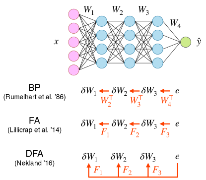
Figure 1: Three approaches to the credit assignment problem in deep neural networks. In back-propagation (BP), the weight updates $\delta W_{l}$ are computed sequentially by transmitting the error $e$ from layer to layer using the transpose of the network’s weights $W_{l}^{\top}$. In feedback alignment (FA) (Lillicrap et al., 2016), $W_{l}^{\top}$ are replaced by fixed random feedback matrices $F_{l}$. In direct feedback alignment (DFA) (Nøkland, 2016), the error is directly injected to each layer using random feedback matrices $F_{l}$, enabling parallelized training.

In light of these shortcomings, algorithms which only approximate the gradient of the loss are attracting increasing interest. Lillicrap et al. (2016) demonstrated that neural networks can be trained successfully even if the transpose of the network weights $W_{l}^{\top}$ are replaced by random feedback connections $F_{l}$ in the backward pass, an algorithm they called “feedback alignment” (FA):

$$\delta a_{l}^{\text{FA}}=\left(F_{l}\delta a_{l+1}\right)\odot g^{\prime}\left(a_{l}\right).$$ (3)

In this way, they dispense with the need of biologically unrealistic symmetric forward and backward weights (Grossberg, 1987; Crick, 1989). The “direct feedback alignment” (DFA) algorithm of Nøkland (2016) takes this idea one step further by propagating the error directly from the output layer to each hidden layer of the network through random feedback connections $F_{l}$:

$$\delta a_{l}^{\text{DFA}}=\left(F_{l}e\right)\odot g^{\prime}\left(a_{l}\right).$$ (4)

DFA thus allows updating different layers in parallel. Fig. 1 shows the information flow of all three algorithms.

While it was initially unclear whether DFA could scale to challenging datasets and complex architectures (Gilmer et al., 2017; Bartunov et al., 2018), recently Launay et al. (2020) obtained performances comparable to fine-tuned BP when using DFA to train a number of state-of-the-art architectures on problems ranging from neural view synthesis to natural language processing. Yet, feedback alignment notoriously fails to train convolutional networks (Bartunov et al., 2018; Moskovitz et al., 2018; Launay et al., 2019; Han & Yoo, 2019). These varied results underline the need for a theoretical understanding of how and when feedback alignment works.

Related Work

Lillicrap et al. (2016) gave a first theoretical characterisation of feedback alignment by arguing that for two-layer linear networks, FA works because the transpose of the second layer of weights $W_{2}$ tends to align with the random feedback matrix $F_{1}$ during training. This weight alignment (WA) leads the weight updates of FA to align with those of BP, leading to gradient alignment (GA) and thus to successful learning. Frenkel et al. (2019) extended this analysis to the deep linear case for a variant of DFA called “Direct Random Target Projection” (DRTP), under the restrictive assumption of training on a single data point. Nøkland (2016) also introduced a layerwise alignment criterion to describe DFA in the deep nonlinear setup, under the assumption of constant update directions for each data point.

Contributions

1. We give an analytical description of DFA dynamics in shallow non-linear networks, building on seminal work analysing BP in the limit of infinitely many training samples (Saad & Solla, 1995a, b; Biehl & Schwarze, 1995).

2. We show that in this setup, DFA proceeds in two steps: an alignment phase, where the forward weights adapt to the feedback weights to improve the approximation of the gradient, is followed by a memorisation phase, where the network sacrifices some alignment to minimise the loss. Out of the same-loss-solutions in the landscape, DFA converges to the one that maximises gradient alignment, an effect we term “degeneracy breaking”.

3. We then focus on the alignment phase in the setup of deep linear networks, and uncover a key quantity underlying GA: the conditioning of the alignment matrices. Our framework allows us to analyse the impact of data structure on DFA, and suggests an explanation for the failure of DFA to train convolutional layers.

4. We complement our theoretical results with experiments that demonstrate the occurence of (i) the Align-then-Memorise phases of learning, (ii) degeneracy breaking and (iii) layer-wise alignment in deep neural networks trained on standard vision datasets.

Reproducibility

We host all the code to reproduce our experiments online at https://github.com/sdascoli/dfa-dynamics.

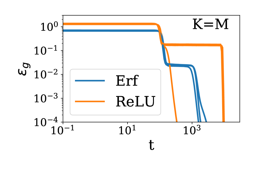
(a) BP, matched

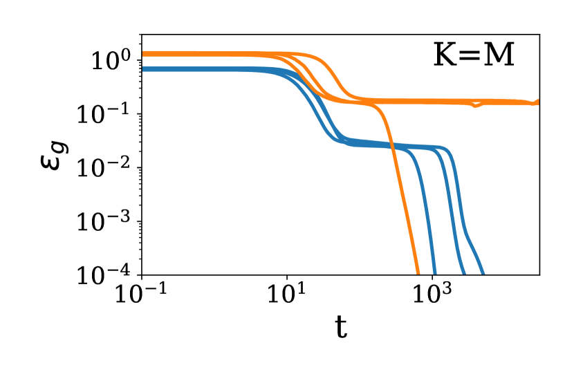
(b) DFA, matched

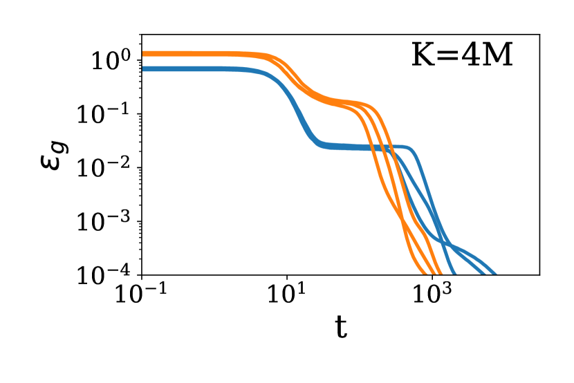
(c) DFA, overparametrized

Figure 2: Learning dynamics of back-propagation and feedback alignment for sigmoidal and ReLU neural networks learning a target function. Each plot shows three runs from different initial conditions for every setting, where a shallow neural network with $K$ hidden nodes tries to learn a teacher network with $M$ hidden nodes. (a) All networks trained using BP in the matched case $K=M$ achieve perfect test error. (b) Sigmoidal networks achieve perfect test error with DFA, but the algorithm fails in some instances to train ReLU networks ($K=M$) (c) In the over-parametrised case ($K>M$), both sigmoidal and ReLU networks achieve perfect generalisation when trained with DFA. Parameters: $N=500,L=2,M=2,\eta=0.1,\sigma_{0}=10^{-2}$.

1 A two-phase learning process

We begin with an exact description of DFA dynamics in shallow non-linear networks. Here we consider a high-dimensional scalar regression task where the inputs $x\in\mathbb{R}^{N}$ are sampled i.i.d. from the standard normal distribution. We focus on the classic teacher-student setup, where the labels $y\in\mathbb{R}$ are given by the outputs of a “teacher” network with random weights (Gardner & Derrida, 1989; Seung et al., 1992; Watkin et al., 1993; Engel & Van den Broeck, 2001; Zdeborová & Krzakala, 2016). In this section, we let the input dimension $N\to\infty$, while both teacher and student are two-layer networks with $K,M\sim O(1)$ hidden nodes.

We consider sigmoidal, $g(x)=\mathrm{erf}\left(\nicefrac{{x}}{{\sqrt{2}}}\right)$, and ReLU activation functions, $g(x)=\max(0,x)$. We asses the student’s performance on the task through its the generalisation error, or test error:

$$\epsilon_{g}(\theta,\tilde{\theta})\equiv\frac{1}{2}\mathbb{E}\,{\left[\hat{y}-y\right]}^{2}\equiv\frac{1}{2}\mathbb{E}\,\left[{e^{2}}\right],$$ (5)

where the expectation $\mathbb{E}\,$ is taken over the inputs for a given teacher and student networks with parameters $\tilde{\theta}=(M,\tilde{W}_{1},\tilde{W}_{2},g)$ and $\theta=(K,W_{1},W_{2},g)$. Learning a target function such as the teacher is a widely studied setup in the theory of neural networks (Zhong et al., 2017; Advani et al., 2020; Tian, 2017; Du et al., 2018; Soltanolkotabi et al., 2018; Aubin et al., 2018; Saxe et al., 2018; Baity-Jesi et al., 2018; Goldt et al., 2019; Ghorbani et al., 2019; Yoshida & Okada, 2019; Bahri et al., 2020; Gabrié, 2020).

In this shallow setup, FA and DFA are equivalent, and only involve one feedback matrix, $F_{1}\in\mathbb{R}^{K}$ which back-propagates the error signal $e$ to the first layer weights $W_{1}$. The updates of the second layer of weights $W_{2}$ are the same as for BP.

Performance of BP vs. DFA

We show the evolution of the test error (5) of sigmoidal and ReLU students trained via vanilla BP in the “matched” case $K=M$ in Fig. 2 a, for three random choices of the initial weights with standard deviation $\sigma_{0}=10^{-2}$. In all cases, learning proceeds in three phases: an initial exponential decay; a phase where the error stays constant, the “plateau” (Saad & Solla, 1995a; Engel & Van den Broeck, 2001; Yoshida & Okada, 2019); and finally another exponential decay towards zero test error.

Sigmoidal students trained by DFA always achieve perfect generalisation when started from different initial weights with a different feedback vector each time (blue in Fig. 2 b) raising a first question: if the student has to align its second-layer weights with the random feedback vector in order to retrieve the BP gradient (Lillicrap et al., 2016), i.e. $W_{2}\propto F_{1}$, how can it recover the teacher weights perfectly, i.e. $W_{2}=\tilde{W}_{2}$?

For ReLU networks, over-parametrisation is key to the consistent success of DFA: while some students with $K=M$ fail to reach zero test error (orange in Fig. 2 b), almost every ReLU student having more parameters than her teacher learns perfectly ($K=4M$ in Fig. 2 c). A second question follows: how does over-parameterisation help ReLU students achieve zero test error?

An analytical theory for DFA dynamics

To answer these two questions, we study the dynamics of DFA in the limit of infinite training data where a previously unseen sample $(x,y)$ is used to compute the DFA weight updates (4) at every step. This “online learning” or “one-shot/single-pass” limit of SGD has been widely studied in recent and classical works on vanilla BP (Kinzel & Ruján, 1990; Biehl & Schwarze, 1995; Saad & Solla, 1995a, b; Saad, 2009; Zhong et al., 2017; Brutzkus & Globerson, 2017; Mei et al., 2018; Rotskoff & Vanden-Eijnden, 2018; Chizat & Bach, 2018; Sirignano & Spiliopoulos, 2019).

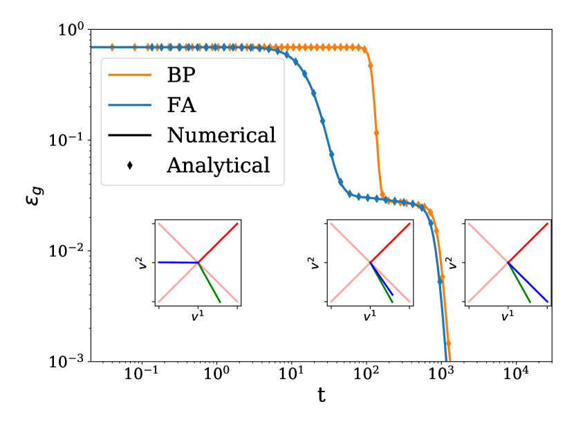
(a) Generalization dynamics

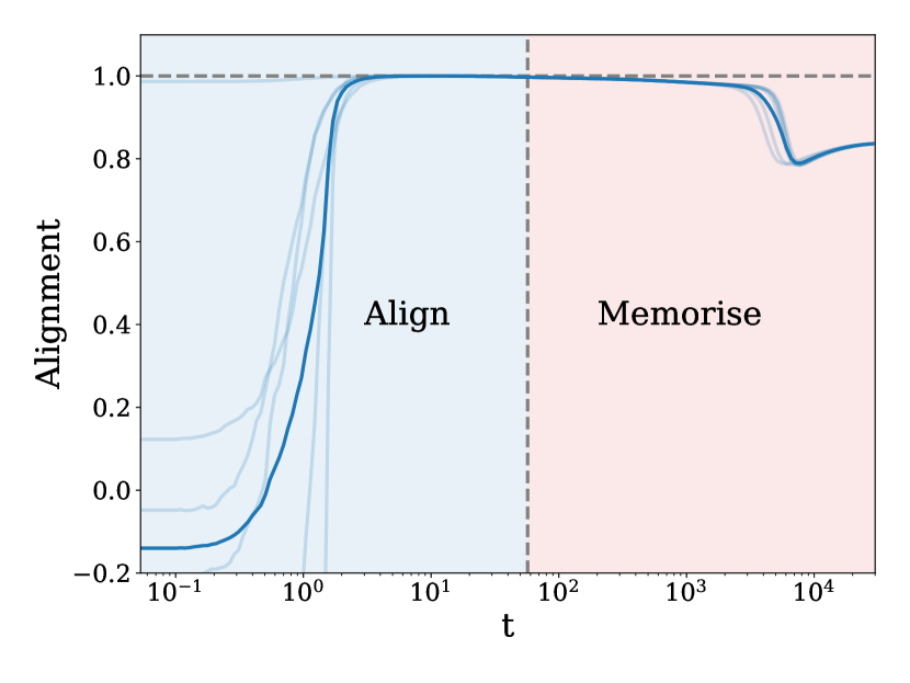
(b) Alignment dynamics

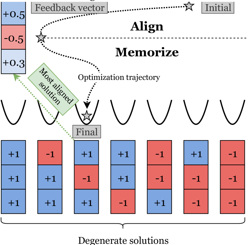
(c) Degeneracy breaking

Figure 3: (a) Theory gives exact prediction for the learning dynamics. We plot learning curves for BP and DFA obtained from (i) a single simulation (solid lines), (ii) integration of the ODEs for BP dynamics (Biehl & Schwarze, 1995; Saad & Solla, 1995a) (orange dots), (iii) integration of the ODEs for DFA derived here (blue dots). Insets: Teacher second-layer weights (red) as well as the degenerate solutions (light red) together with the feedback vector $F_{1}$ (green) and the student second-layer weights $v$ (blue) at three different times during training with DFA. Parameters: $N=500,K=M=2,\eta=0.1,\sigma_{0}=10^{-2}$.
(b) Align-then-Memorise process. Alignment (cosine similarity) between the student’s second layer weights and the feedback vector. In the align phase, the alignment increases, and reaches its maximal value when the test loss reaches the plateau. Then it decreases in the memorization phase, as the student recovers the teacher weights.
(c) The degeneracy breaking mechanism. There are multiple degenerate global minima in the optimisation landscape: they are related through a discrete symmetry transformation of the weights that leaves the student’s output unchanged. DFA chooses the solution which maximises the alignment with the feedback vector.

We work in the regime where the input dimension $N\to\infty$, while $M$ and $K$ are finite. The test error (5), i.e. a function of the student and teacher parameters involving a high-dimensional average over inputs, can be simply expressed in terms of a finite number of “order parameters” $Q=(Q^{kl}),R=(R^{km}),T=(T^{mn})$,

$$\lim_{N\to\infty}\epsilon_{g}(\theta,\tilde{\theta})=\epsilon_{g}(Q,R,T,W_{2},\tilde{W}_{2})$$ (6)

where

$$Q^{kl}\!=\!\frac{W_{1}^{k}W_{1}^{l}}{N},\text{ }R^{km}\!=\!\frac{W_{1}^{k}\tilde{W}_{1}^{m}}{N},\text{ }T^{mn}\!=\!\frac{\tilde{W}_{1}^{m}\tilde{W}_{1}^{n}}{N}$$ (7)

as well as second layer weights $\tilde{W}_{2}^{m}$ and $W_{2}^{k}$ (Saad & Solla, 1995a, b; Biehl & Schwarze, 1995; Engel & Van den Broeck, 2001). Intuitively, $R^{km}$ quantifies the similarity between the weights of the student’s $k$th hidden unit and the teacher’s $m$th hidden unit. The self-overlap of the $k$th and $l$th student nodes is given by $Q^{kl}$, and likewise $T^{mn}$ gives the (static) self-overlap of teacher nodes. In seminal work, Saad & Solla (1995a) and Biehl & Schwarze (1995) obtained a closed set of ordinary differential equations (ODEs) for the time evolution of the order parameters $Q$ and $R$. Our first main contribution is to extend their approach to the DFA setup (see SM A for the details), obtaining a set of ODEs (27) that predicts the test error of a student trained using DFA (4) at all times. The accuracy of the predictions from the ODEs is demonstrated in Fig. 3 a, where the comparison between a single simulation of training a two-layer net with BP (orange) and DFA (blue) and theoretical predictions yield perfect agreement.

1.1 Sigmoidal networks learn through “degeneracy breaking”

The test loss of a sigmoidal student trained on a teacher with the same number of neurons as herself ($K=M$) contains several global minima, which all correspond to fixed points of the ODEs (27). Among these is a student with exactly the same weights as her teacher. The symmetry $\mathrm{erf}(z)=-\mathrm{erf}(-z)$ induces a student with weights $\{\tilde{W}_{1},\tilde{W}_{2}\}$ to have the same test error as a sigmoidal student with weights $\{-\tilde{W}_{1},-\tilde{W}_{2}\}$. Thus, as illustrated in Fig. 3 c, the problem of learning a teacher has various degenerate solutions. A student trained with vanilla BP converges to any one of these solutions, depending on the initial conditions.

Alignment phase

A student trained using DFA has to fulfil the same objective (zero test error), with an additional constraint: her second-layer weights $W_{2}$ need to align with the feedback vector $F_{1}$ to ensure the first-layer weights are updated in the direction that minimises the test error. And indeed, an analysis of the ODEs (cf. Sec. B) reveals that in the early phase of training, $\dot{W_{2}}\sim F$ and so $W_{2}$ grows in the direction of the feedback vector $F_{1}$ resulting in an increasing overlap between $W_{2}$ and $F_{1}$. In this alignment phase of learning, shown in Fig. 3 b, $W_{2}$ becomes perfectly aligned with $F_{1}$. DFA has perfectly recovered the weight updates for $W_{1}$ of BP, but the second layer has lost its expressivity (it is simply aligned to the random feedback vector).

Memorisation phase

The expressivity of the student is restored in the memorisation phase of learning, where the second layer weights move away from $F_{1}$ and towards the global miminum of the test error that maintains the highest overlap with the feedback vector. In other words, students solve this constrained optimisation problem by consistently converging to the global minimum of the test loss that simultaneously maximises the overlap between $W_{2}$ and $F_{1}$, and thus between the DFA gradient and the BP gradient. For DFA, the global minima of the test loss are not equivalent, this “degeneracy breaking” is illustrated in Fig. 3 c.

1.2 Degeneracy breaking requires over-parametrisation for ReLU networks

The ReLU activation function possesses the continuous symmetry $\max(0,x)=\gamma\max(0,x/\gamma)$ for any $\gamma>0$ preventing ReLU networks to compensate a change of sign of $W_{2}^{k}$ with a change of sign of $W_{1}^{k}$. Consequently, a ReLU student can only simultaneously align to the feedback vector $F_{1}$ and recover the teacher’s second layer $\tilde{W}_{2}$ if at least $M$ elements of $F_{1}$ have the same sign as $\tilde{W}_{2}$. The inset of Fig. 4 shows that a student trained on a teacher with $M=2$ second-layer weights $\tilde{W}_{2}^{m}=1$ only converges to zero test error if the feedback vector has 2 positive elements (green). If instead the feedback vector has only 0 (blue) or 1 (orange) positive entry, the student will settle at a finite test error. More generally, the probability of perfect recovery for a student with $K\geq M$ nodes sampled randomly is given analytically as:

$$P(\text{learn})=\frac{1}{2^{K}}\sum_{k=0}^{M}\binom{K}{k}.$$ (8)

As shown in Fig. 4, this formula matches with simulations. Note that the importance of the “correct” sign for the feedback matrices was also observed in deep neural networks by Liao et al. (2016).

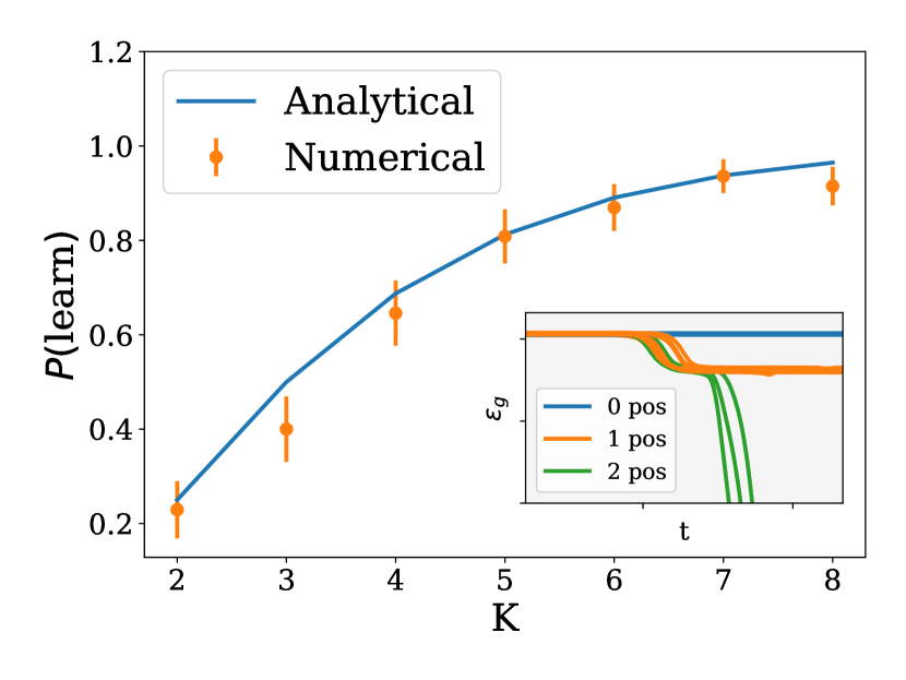
Figure 4: Over-parameterisation improves performance of shallow ReLU networks. We show the learning dynamics of a student with $K=3$ hidden nodes trained on a teacher with $M=2$ nodes and $\tilde{W}_{2}^{m}=1$ if the feedback vector has 0, 1, or 2 positive entries. Inset: Probability of achieving zero test error (Eq. 8, line) compared to the fraction of simulations that converged to zero test error (out of 50, crosses). Other parameters: $N=500,\eta=0.1,\sigma_{0}=10^{-2}$.

1.3 Degeneracy breaking in deep networks

We explore to what extent degeneracy breaking occurs in deep nonlinear networks by training 4-layer multi-layer perceptrons (MLPs) with 100 nodes per layer for 1000 epochs with both BP and DFA, on the MNIST and CIFAR10 datasets, with Tanh and ReLU nonlinearities (cf. App. E.2 for further experimental details). The dynamics of the training loss, shown in the left of Fig. 5, are very similar for BP and DFA.

From degeneracy breaking, one expects DFA to drive the optimization path towards a special region of the loss landscape determined by the feedback matrices. We test this hypothesis by measuring whether networks trained with the same feedback matrices from different initial weights converge towards the same region of the landscape. The cosine similarity between the vectors obtained by stacking the weights of two networks trained independently using BP reaches at most $10^{-2}$ (right of Fig. 5), signalling that they reach very distinct minima. In contrast, when trained with DFA, networks reach a cosine similarity between $0.5$ and $1$ at convergence, thereby confirming that DFA breaks the degeneracy between the solutions in the landscape and biases towards a special region of the loss landscape, both for sigmoidal and ReLU activation functions.

This result suggests that heavily over-parametrised neural networks used in practice can be trained successfully with DFA because they have a large number of degenerate solutions. We leave a more detailed exploration of the interplay between DFA and the loss landscape for future work. As we discuss in Sec. 3 the Align-then-Memorise mechanism sketched in Fig. 3 c also occurs in deep non-linear networks.

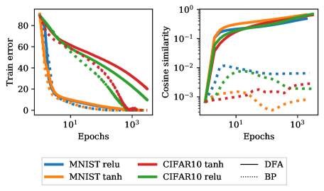
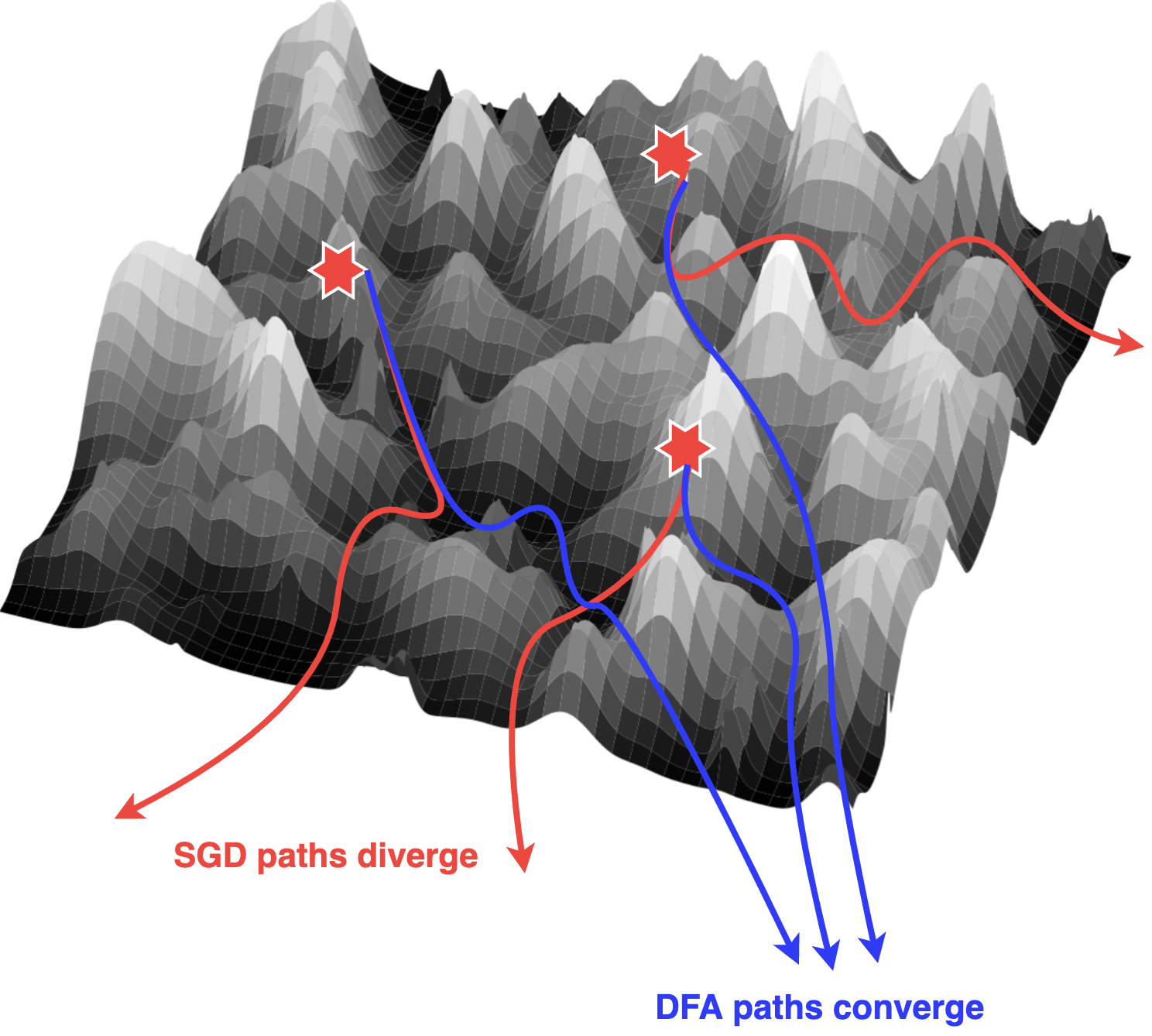
Figure 5: Degeneracy breaking also occurs in deep neural networks. (Left) We plot the training accuracy and the cosine similarity between the weights of four-layer fully-connected neural networks with sigmoidal and ReLU activations during training on MNIST and CIFAR10. Averages taken over 10 runs; for exp. details see Sec. 1.3. (Right) Cartoon of the degeneracy breaking process in the loss landscape of a deep network: while the optimization paths of models trained with SGD diverge in the loss landscape, with DFA they converge to a region of the landscape determined by the feedback matrices.

2 How do gradients align in deep networks?

This section focuses on the alignment phase of learning. In the two-layer setup there is a single feedback vector $F_{1}$, of same dimensions as the second layer $W_{2}$, and to which $W_{2}$ must align in order for the first layer to recover the true gradient.

In deep networks, as each layer $W_{l}$ has a distinct feedback matrix $F_{l}$ of different size of $W_{l}$, it is not obvious how the weights must align to ensure gradient alignment. We study how the alignment occurs by considering deep linear networks with $L$ layers without bias, without any assumption on the training data. While the expressivity of linear networks is naturally limited, their learning dynamics is non-linear and rich enough to give insights that carry over to the non-linear case both for BP (Baldi & Hornik, 1989; Le Cun et al., 1991; Krogh & Hertz, 1992; Saxe et al., 2014; Advani et al., 2020) and for DFA (Lillicrap et al., 2016; Nøkland, 2016; Frenkel et al., 2019).

2.1 Weight alignment as a natural structure

In the following, we assume that the weights are initialised to zero. With BP, they would stay zero at all times, but for DFA the layers become nonzero sequentially, from the bottom to the top layer. In the linear setup, the updates of the first two layers at time $t$ can be written in terms of the corresponding input and error vectors using Eq. (4):

$$\delta W_{1}^{t}=-\eta(F_{1}e_{t})x_{t}^{T},\quad\delta W_{2}^{t}=-\eta(F_{2}e_{t}){(W_{1}x_{t})}^{\top}$$ (9)

Summing these updates shows that the first layer performs Hebbian learning modulated by the feedback matrix $F_{1}$:

$$W_{1}^{t} =-\eta\sum\nolimits_{t^{\prime}=0}^{t-1}F_{1}e_{t^{\prime}}x_{t^{\prime}}^{\top}=F_{1}A_{1}^{t},$$ (10)

$$A_{1}^{t} =-\eta\sum\nolimits_{t^{\prime}=0}^{t-1}e_{t^{\prime}}x_{t^{\prime}}^{\top}$$ (11)

Plugging this result into $\delta W_{2}^{t}$, we obtain:

$$W_{2}^{t} =-\eta\sum_{t^{\prime}=0}^{t-1}F_{2}e_{t}(A_{1}^{t^{\prime}}x_{t^{\prime}})^{\top}F_{1}^{\top}=F_{2}A_{2}^{t}F_{1}^{\top},$$ (12)

$$A_{2}^{t} =\eta^{2}\sum_{t^{\prime}=0}^{t-1}\sum_{t^{\prime\prime}=0}^{t^{\prime}-1}(x_{t^{\prime}}\cdot x_{t^{\prime\prime}})e_{t^{\prime}}e_{t^{\prime\prime}}^{\top}.$$ (13)

When iterated, the procedure above reveals that DFA naturally leads to weak weight alignment of the network weights to the feedback matrices:

$$\text{{Weak WA: }}W_{1<l<L}^{t}\!=\!F_{l}A_{l}^{t}F_{l-1}^{\top}\!,\quad W_{L}^{t}\!=\!A_{L}^{t}F_{L-1}^{\top},$$ (14)

where we defined the alignment matrices $A_{l\geq 2}^{t}\in\mathbb{R}^{n_{L}\times n_{L}}$:

$$A_{l\geq 2}^{t}=\eta^{2}\sum_{t^{\prime}=0}^{t-1}\sum_{t^{\prime\prime}=0}^{t^{\prime}-1}(B_{l}^{t^{\prime}}x_{t^{\prime}})\cdot(B_{l}^{t^{\prime\prime}}x_{t^{\prime\prime}})e_{t^{\prime}}e_{t^{\prime\prime}}^{\top}.$$ (15)

$B_{l}\in\mathbb{R}^{n_{L}\times n_{L}}$ is defined recursively as a function of the feedback matrices only and its expression together with the full derivation is deferred to App. C. These results can be adapted both to DRTP (Frenkel et al., 2019), another variant of feedback alignment where $e_{t}=-y_{t}$ and to FA by performing the replacement $F_{l}\to F_{l}F_{l+1}\ldots F_{L-1}$.

2.2 Weight alignment leads to gradient alignment

Weak WA builds throughout training, but does not directly imply GA. However, if the alignment matrices become proportional to the identity, we obtain strong weight alignment:

$$\mathrm{\textbf{Strong WA:}}\quad W_{1<l<L}^{t}\propto F_{l}F_{l-1}^{\top},\quad W_{L}^{t}\propto F_{L-1}^{\top}.$$ (16)

Additionally, since GA requires $F_{l}e\propto W_{l+1}^{\top}\delta a_{l+1}$ (Eqs. 4 and 2), strong WA directly implies GA if the feedback matrices $F_{l\geq 2}$ are assumed left-orthogonal, i.e. $F_{l}^{\top}F_{l}=\mathbb{I}_{n_{L}}$. Strong WA of (16) induces the weights, by the orthogonality condition, to cancel out by pairs of two:

$$W_{l+1}^{\top}\delta a_{l+1} \propto F_{l}F_{l+1}^{\top}F_{l+1}\ldots F_{L-1}^{\top}F_{L-1}e=F_{l}e.$$ (17)

The above suggests that taking the feedback matrices left-orthogonal is favourable for GA. If the feedback matrices elements are sampled i.i.d. from a Gaussian distribution, GA still holds in expectation since $\mathbb{E}\left[F_{l}^{\top}F_{l}\right]\propto\mathbb{I}_{n_{L}}$.

Quantifying gradient alignment

Our analysis shows that key to GA are the alignment matrices: the closer they are to identity, i.e. the better their conditioning, the stronger the GA. This comes at the price of restricted expressivity, since layers are encouraged to align to a product of (random) feedback matrices. In the extreme case of strong WA, the freedom of layers $l\geq 2$ is entirely sacrificed to allow learning in the first layer! This is not harmful for the linear networks as the first layer alone is enough to maintain full expressivity. Nonlinear networks, as argued in Sec. 1, rely on the Degeneracy Breaking mechanism to recover expressivity.

3 The case of deep nonlinear networks

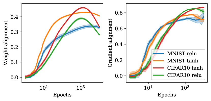
Figure 6: Global alignment dynamics of deep nonlinear networks exhibits Align-then-Memorise. Global weight and gradient alignments, as defined in (18), varying the activation function and the dataset. Shaded regions represent the (small) variability over 10 runs.

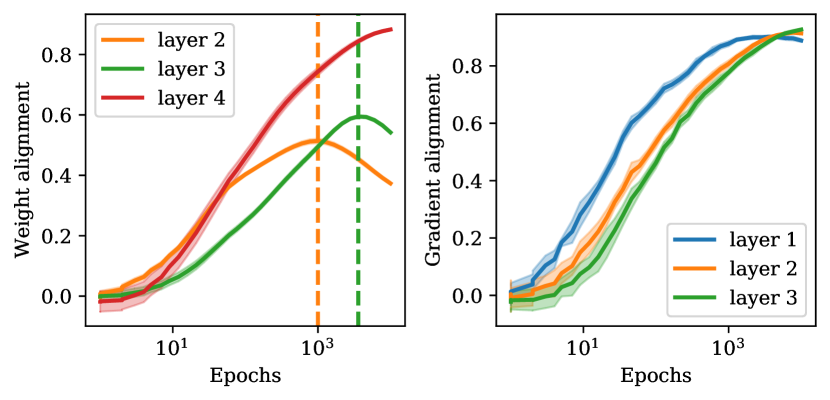
Figure 7: Layerwise alignment dynamics reveal sequential Align-then-Memorise. Layerwise weight and gradient alignments as defined in (19), for a ReLU network trained on CIFAR10 with 10% label corruption. Shaded regions represent the (small) variability over 10 runs.

In this section, we show that the theoretical predictions of the previous two sections hold remarkably well in deep nonlinear networks trained on standard vision datasets.

3.1 Weight Alignment occurs like in the linear setup

To determine whether WA described in Sec. 2 holds in the deep nonlinear setup of Sec. 1.3, we introduce the global and layerwise alignment observables:

$$\mathrm{WA}\!=\!\measuredangle\left(\mathbf{F},\mathbf{W}\right)\!, \mathrm{GA}\!=\!\measuredangle\left(\mathbf{G}^{\mathrm{DFA}},\mathbf{G}^{\mathrm{BP}}\right)$$ (18)

$$\mathrm{WA}_{l\geq 2}\!=\!\measuredangle\!\left(\mathbf{F}_{l}\!,\!\mathbf{W}_{l}\right)\!, \mathrm{GA}_{l\geq 2}\!=\!\measuredangle\left(\mathbf{G}^{\mathrm{DFA}}_{l}\!,\!\mathbf{G}^{\mathrm{BP}}_{l}\right),$$ (19)

where $\measuredangle(\mathbf{A},\mathbf{B})=\mathrm{Vec}(\mathbf{A})\cdot\mathrm{Vec}(\mathbf{B})/\|\mathbf{A}\|\|\mathbf{B}\|$ and

$$\mathbf{F} =\left(F_{2}F_{1}^{\top},\ldots,F_{L-1}F_{L-2}^{\top},F_{L-1}^{\top}\right),$$

$$\mathbf{W}(t) =\left(W_{2}^{t},\ldots,W_{L-1}^{t},W_{L}^{t}\right),$$

$$\mathbf{G}(t) =\left(\delta a_{1}^{t},\ldots,\delta a_{L-1}^{t}\right).$$

Note that the layer-wise alignment of $W_{l}$ with $F_{l}F_{l-1}^{\top}$ was never measured before: it differs from the alignment of $F_{l}$ with $W_{l+1}\ldots W_{L}$ observed in (Crafton et al., 2019), which is more akin to GA.

If $\mathbf{W}$ and $\mathbf{F}$ were uncorrelated, the WA defined in (18) would be vanishing as the width of the layer grows large. Remarkably, WA becomes of order one after a few epochs as shown in Fig. 6 (left), and strongly correlates with GA (right). This suggests that the layer-wise WA uncovered for linear networks with weights initialized to zero also drives GA in the general case.

3.2 Align-then-Memorise occurs from bottom layers to top

As can be seen in Fig. 6, WA clearly reaches a maximum then decreases, as expected from the Align-then-Memorise process. Notice that the decrease is stronger for CIFAR10 than it is for MNIST, since CIFAR-10 is much harder to fit than MNIST: more WA needs to be sacrificed. Increasing label corruption similarly makes the datasets harder to fit, and decreases the final WA, as detailed in SM E.2. However, another question arises: why does the GA keep increasing in this case, in spite of the decreasing WA?

To answer this question, we need to disentangle the dynamics of the layers of the network, as in Eq. (19). In Fig. 7, we focus on the ReLU network applied to CIFAR10, and shuffle 10% of the labels in the training set to make the Align-then-Memorise procedure more easily visible. Although the network contains 4 layers of weights, we only have 3 curves for WA and GA: WA is only defined for layers 2 to 4 according to Eq. (19), whereas GA of the last layer is not represented here since it is always equal to one.

As can be seen, the second layer is the first to start aligning: it reaches its maximal WA around $1000$ epochs (orange dashed line), then decreases. The third layer starts aligning later and reaches its maximal WA around $2000$ epochs (green dashed line), then decreases. As for the last layer, the WA is monotonically increasing. Hence, the Align-then-Memorise mechanism operates in a layerwise fashion, starting from the bottom layers to the top layers.

Note that the WA of the last layers is the most crucial, since it affects the GA of all the layers below, whereas the WA of the second layer only affects the GA of the first layer. It therefore makes sense to keep the WA of the last layers high, and let the bottom layers perform the memorization first. This is reminiscent of the linear setup, where all the layers align except for the first, which does all the learning. In fact, this strategy enables the GA of each individual layer to keep increasing until late times: the diminishing WA of the bottom layers is compensated by the increasing WA of the top layers.

4 What can hamper alignment?

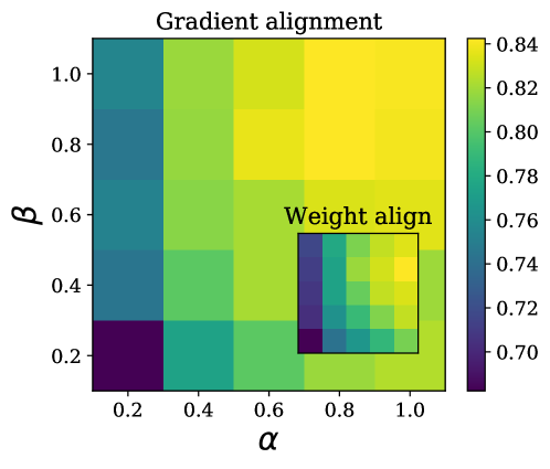
Figure 8: Badly conditioned output statistics can hamper alignment. WA and GA at the final point of training decrease when the output classes are correlated ($\beta<1$) or of different variances ($\alpha<1$).

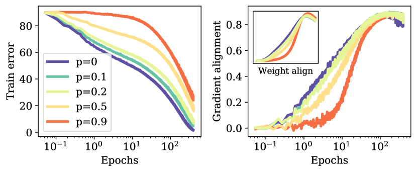
Figure 9: Label corruption hampers alignment in the early stages of training. We see that the higher the label corruption, the more time WA and GA take to start increasing, since the network initially predicts equal probabilities over the output classes.

We demonstrated that GA is enabled by the WA mechanism, both theoretically for linear networks and numerically for nonlinear networks. In this section, we leverage our analysis of WA to identify situations in which GA fails.

4.1 Alignment is data-dependent

In the linear case, GA occurs if the alignment matrices presented in Sec. 2 are well conditioned. Note that if the output size $n_{L}$ is equal to one, e.g. for scalar regression or binary classification tasks, then the alignment matrices are simply scalars, and GA is guaranteed. When this is not the case, one can obtain the deviation from GA by studying the expression of the alignment matrices (15). They are formed by summing outer products of the error vectors $e_{t^{\prime}}e_{t^{\prime\prime}}^{\top}$, where $e_{t}=\hat{y}_{t}\!-\!y_{t}$. Therefore, good conditioning requires the different components of the errors to be uncorrelated and of similar variances. This can be violated by (i) the targets $y$, or (ii) the predictions $\hat{y}$.

(i) Structure of data

The first scenario can be demonstrated in a simple regression task on i.i.d. Gaussian inputs $x\sim\mathbb{R}^{10}$. The targets $y\in\mathbb{R}^{2}$ are randomly sampled from the following distribution:

$$y\!\sim\!\mathcal{N}(0,\Sigma),\quad\Sigma\!=\!\begin{pmatrix}1&\alpha(1-\beta)\\ \alpha(1-\beta)&\alpha^{2}\end{pmatrix}\!,\!\!\quad\alpha,\beta\!\leq 1.$$ (20)

In Fig. 8, we show the final WA and GA of a 3-layer ReLU network trained for $10^{3}$ epochs on $10^{3}$ examples sampled from this distribution (further details in SM E.3). As predicted, imbalanced ($\alpha<1$) or correlated ($\beta<1$) target statistics hamper WA and GA. Note that the inputs also come into play in Eq. (15): a more detailed theoretical analysis of the impact of input and target statistics on alignment is deferred to SM D.

(ii) Effect of noise

For classification tasks, the targets $y$ are one-hot encodings whose statistics are naturally well conditioned. However, alignment can be degraded if the statistics of the predictions $\hat{y}$ become correlated.

One can enforce such a correlation in CIFAR10 by shuffling a fraction $p$ of the labels. The WA and GA dynamics of a 3-layer ReLU network are shown in Fig. 9. At high $p$, the network can only perform random guessing during the first few epochs, and assigns equal probabilities to the 10 classes. The correlated structure of the predictions prevents alignment until the network starts to fit the random labels: the predictions of the different classes then decouple and WA takes off, leading to GA.

4.2 Alignment is impossible for convolutional layers

A convolutional layer with filters $H_{l}$ can be represented by a large fully-connected layer whose weights are represented by a block Toeplitz matrix $\phi(H_{l})$ (d’Ascoli et al., 2019). This matrix has repeated blocks due to weight sharing, and most of its weights are equal to zero due to locality. In order to verify WA and therefore GA, the following condition must hold: $\phi(H_{l})\propto F_{l}F_{l-1}^{\top}$. Yet, due to the very constrained structure of $\phi(H_{l})$, this is impossible for a general choice of $F_{l}$. Therefore, the WA mechanism suggests a simple explanation for why GA doesn’t occur in vanilla CNNs, and confirms the previously stated hypothesis that CNNs don’t have enough flexibility to align (Launay et al., 2019).

In the case of convolutional layers, this lack of alignment makes learning near to impossible, and has lead practitioners to design alternatives (Han & Yoo, 2019; Moskovitz et al., 2018). However, the extent to which alignment correlates with good performance in the general setup (both in terms of fitting and generalisation) is a complex question which we leave for future work. Indeed, nothing prevents DFA from finding a good optimization path, different from the one followed by BP. Conversely, obtaining high gradient alignment at the end of training is not a sufficient condition for DFA to retrieve the results of BP, e.g. if the initial trajectory leads to a wrong direction.

Appendix A Derivation of the ODE

The derivation of the ODE’s that describe the dynamics of the test error for shallow networks closely follows the one of Saad & Solla (1995a) and Biehl & Schwarze (1995) for back-propagation. Here, we give the main steps to obtain the analytical curves of the main text and refer the reader to their paper for further details.

As we discuss in Sec. 1, student and teacher are both two-layer networks with $K$ and $M$ hidden nodes, respectively. For an input $x\in\mathbb{R}^{N}$, their outputs $\hat{y}$ and $y$ can be written as

$$\hat{y} =\phi_{\theta}(x)=\sum_{k=1}^{K}W_{2}^{k}\,g\left(\lambda^{k}\right),$$

$$y =\phi_{\tilde{\theta}}(x)=\sum_{m=1}^{M}\tilde{W}_{2}^{m}\,g\left(\nu^{m}\right),$$ (21)

where we have introduced the pre-activations $\lambda^{k}\equiv W_{1}^{k}x/\sqrt{N}$ and $\nu^{m}\equiv\tilde{W}_{1}^{m}x/\sqrt{N}$. Evaluating the test error of a student with respect to the teacher under the squared loss leads us to compute the average

$$\epsilon_{g}\left(\theta,\tilde{\theta}\right)=\frac{1}{2}\mathbb{E}\,_{x}\left[\sum_{k=1}^{K}W_{2}^{k}\,g\left(\lambda^{k}\right)-\sum_{m=1}^{M}\tilde{W}_{2}^{m}\,g\left(\nu^{m}\right)\right]^{2},$$ (22)

where the expectation is taken over inputs $x$ for a fixed student and teacher. Since $x$ only enters Eq. (22) via the pre-activations $\lambda=(\lambda^{k})$ and $\nu=(\nu^{m})$, we can replace the high-dimensional average over $x$ by a low-dimensional average over the $K+M$ variables $(\lambda,\nu)$. The pre-activations are jointly Gaussian since the inputs are drawn element-wise i.i.d. from the Gaussian distribution. The mean of $(\lambda,\nu)$ is zero since $\mathbb{E}\,x_{i}=0$, so the distribution of $(\lambda,\nu)$ is fully described by the second moments

$$Q^{kl}=\mathbb{E}\,\lambda^{k}\lambda^{l}=W_{1}^{k}\cdot W_{1}^{l}/N,$$ (23)

$$R^{km}=\mathbb{E}\,\lambda^{k}\nu^{m}=W_{1}^{k}\cdot\tilde{W}_{1}^{m}/N,$$ (24)

$$T^{mn}=\mathbb{E}\,\nu^{m}\nu^{n}=\tilde{W}_{1}^{m}\cdot\tilde{W}_{1}^{n}/N.$$ (25)

which are the “order parameters” that we introduced in the main text. We can thus rewrite the generalisation error (5) as a function of only the order parameters and the second-layer weights,

$$\lim_{N\to\infty}\epsilon_{g}(\theta,\tilde{\theta})=\epsilon_{g}(Q,R,T,W_{2},\tilde{W}_{2})$$ (26)

As we update the weights using SGD, the time-dependent order parameters $Q,R$, and $W_{2}$ evolve in time. By choosing different scalings for the learning rates in the SGD updates (4), namely

$$\eta_{W_{1}}=\eta,\qquad\eta_{W_{2}}=\eta/N$$

for some constant $\eta$, we guarantee that the dynamics of the order parameters can be described by a set of ordinary differential equations, called their “equations of motion”. We can obtain these equations in a heuristic manner by squaring the weight update (4) and taking inner products with $\tilde{W}_{1}^{m}$, to yield the equations of motion for $Q$ and $R$ respectively:

$$\frac{\operatorname{d}\!R^{km}}{\operatorname{d}\!\alpha} =-\eta F_{1}^{k}\mathbb{E}\,\left[g^{\prime}(\lambda^{k})\nu^{m}e\right]$$ (27a)

$$\frac{\operatorname{d}\!Q^{k\ell}}{\operatorname{d}\!\alpha} =-\eta F_{1}^{k}\mathbb{E}\,\left[g^{\prime}(\lambda^{k})\lambda^{\ell}e\right]-\eta F_{1}^{\ell}\mathbb{E}\,\left[g^{\prime}(\lambda^{\ell})\lambda^{k}e\right]$$

$$+\eta^{2}F_{1}^{k}F_{1}^{\ell}\mathbb{E}\,\left[g^{\prime}(\lambda^{k})g^{\prime}(\lambda^{\ell})e^{2}\right],$$ (27b)

$$\frac{\operatorname{d}\!W_{2}^{k}}{\operatorname{d}\!\alpha} =-\eta\mathbb{E}\,\left[g(\lambda^{k})e\right]$$ (27c)

where, as in the main text, we introduced the error $e=\phi_{\theta}(x)-\phi_{\tilde{\theta}}(x)$. In the limit $N\to\infty$, the variable $\alpha=\mu/N$ becomes a continuous time-like variable. The remaining averages over the pre-activations, such as

$$\mathbb{E}\,g^{\prime}(\lambda^{k})\lambda^{\ell}g(\nu^{m}),$$

are simple three-dimensional integral over the Gaussian random variables $\lambda^{k},\lambda^{\ell}$ and $\nu^{m}$ and can be evaluated analytically for the choice of $g(x)=\mathrm{erf}(x/\sqrt{2})$ (Biehl & Schwarze, 1995) and for linear networks with $g(x)=x$. Furthermore, these averages can be expressed only in term of the order parameters, and so the equations close. We note that the asymptotic exactness of Eqs. 27 can be proven using the techniques used recently to prove the equations of motion for BP (Goldt et al., 2019).

We provide an integrator for the full system of ODEs for any $K$ and $M$ in the Github repository.

Appendix B Detailed analysis of DFA dynamics

In this section, we present a detailed analysis of the ODE dynamics in the matched case $K=M$ for sigmoidal networks ($g(x)=\mathrm{erf}\left(\nicefrac{{x}}{{\sqrt{2}}}\right)$).

The Early Stages and Gradient Alignment

We now use Eqs. (27) to demonstrate that alignment occurs in the early stages of learning, determining from the start the solution DFA will converge to (see Fig. 3 which summarises the dynamical evolution of the student’s second layer weights).

Assuming zero initial weights for the student and orthogonal first layer weights for the teacher (i.e. $T^{nm}$ is the identity matrix), for small times ($t\ll 1$), one can expand the order parameters in $t$:

$$R^{km}(t) =t\dot{R}^{km}(0)+\mathcal{O}(t^{2}),$$

$$Q^{kl}(t) =t\dot{Q}^{kl}(0)+\mathcal{O}(t^{2}),$$

$$W_{2}^{k}(t) =t\dot{W}_{2}^{k}(0)+\mathcal{O}(t^{2}).$$ (28)

where, due to the initial conditions, $R(0)=Q(0)=W_{2}(0)=0$. Using Eq. 27, we can obtain the lowest order term of the above updates:

$$\dot{R}^{km}(0) =\frac{\sqrt{2}}{\pi}\eta\tilde{W}_{2}^{m}F_{1}^{k},$$

$$\dot{Q}^{kl}(0) =\frac{2}{\pi}\eta^{2}\left((\tilde{W}_{2}^{k})^{2}+(\tilde{W}_{2}^{l})^{2}\right)F_{1}^{l}F_{1}^{k},$$

$$\dot{W}_{2}^{k}(0) =0$$ (29)

Since both $\dot{R}(0)$ and $\dot{Q}(0)$ are non-zero, this initial condition is not a fixed point of DFA. To analyse initial alignment, we consider the first order term of $\dot{W}_{2}$. Using Eq. (28) with the derivatives at $t=0$ (B), we obtain to linear order in $t$:

$$\dot{W}_{2}^{k}(t)= \frac{2}{\pi^{2}}\eta^{2}||\tilde{W}_{2}||^{2}F_{1}^{k}t.$$ (30)

Crucially, this update is in the direction of the feedback vector $F_{1}$. DFA training thus constrains the student to initially grow in the direction of the feedback vector and align with it. This implies gradient alignment between BP and DFA and dictates into which of the many degenerate solutions in the energy landscape the student converges.

Plateau phase

After the initial phase of learning with DFA where the test error decreases exponentially, similarly to BP, the student falls into a symmetric fixed point of the Eqs. (27) where the weights of a single student node are correlated to the weights of all the teacher nodes ((Saad & Solla, 1995a; Biehl & Schwarze, 1995; Engel & Van den Broeck, 2001)). The test error stays constant while the student is trapped in this fixed point. We can obtain an analytic expression for the order parameters under the assumption that the teacher first-layer weights are orthogonal ($T^{nm}=\delta_{nm}$). We set the teacher’s second-layer weights to unity for notational simplicity ($\tilde{W}_{2}^{m}=1$) and restrict to linear order in the learning rate $\eta$, since this is the dominant contribution to the learning dynamics at early times and on the plateau (Saad & Solla, 1995b). In the case where all components of the feedback vector are positive, the order parameters are of the form $Q^{kl}=q,R^{km}=r,W_{2}^{k}=w_{2}$ with:

$$q=\frac{1}{2K-1},\quad r=\sqrt{\frac{q}{2}},\quad w_{2}=\sqrt{\frac{1+2q}{q(4+3q)}}.$$ (31)

If the components of the feedback vector are not all positive, we instead obtain $R^{km}=\operatorname{sgn}(F^{k})r$, $W_{2}^{k}=\operatorname{sgn}(F^{k})w_{2}$ and $Q^{kl}=\operatorname{sgn}(F^{k})\operatorname{sgn}(F^{l})q$. This shows that on the plateau the student is already in the configuration that maximises its alignment with $F_{1}$. Note that in all cases, the value of the test error reached at the plateau is the same for DFA and BP.

Memorisation phase and Asymptotic Fixed Point

At the end of the plateau phase, the student converges to its final solution, which is often referred to as the specialised phase (Saad & Solla, 1995a; Biehl & Schwarze, 1995; Engel & Van den Broeck, 2001). The configuration of the order parameters is such that the student reproduces her teacher up to sign changes that guarantee the alignment between $W_{2}$ and $F_{1}$ is maximal, i.e. $\operatorname{sgn}(W^{k}_{2})=\operatorname{sgn}(F_{1}^{k})$. The final value of the test error of a student trained with DFA is the same as that of a student trained with BP on the same teacher.

Choice of the feedback vector

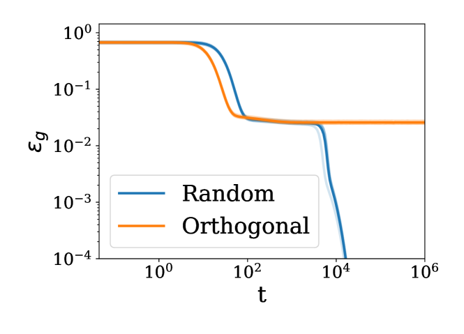
Figure 10: Test error of a sigmoidal student started with zero initial weights. The feedback vector $F_{1}$ is chosen random (blue) and orthogonal to the teacher’s second layer weights $\tilde{W}_{2}$ (orange). Parameters: $\eta=0.1,K=M=2$.

In the main text, we saw how a wrong choice of feedback vector $F_{1}$ can prevent a ReLU student from learning a task. Here, we show that also for sigmoidal student, a wrong choice of feedback vector $F_{1}$ is possible. As Fig. 10 shows, in the case where the $F_{1}$ is taken orthogonal to the teacher second layer weights, a student whose weights are initialised to zero remains stuck on the plateau and is unable to learn. In contrast, when the $F_{1}$ is chosen with random i.i.d. components drawn from the standard normal distribution, perfect recovery is achieved.

Appendix C Derivation of weight alignment

Since the network is linear, the update equations are (consider the first three layers only):

$$\delta W_{1} =-\eta(F_{1}e)x^{T},$$ (32)

$$\quad\delta W_{2} =-\eta(F_{2}e)(W_{1}x)^{\top},$$ (33)

$$\delta W_{3} =-\eta(F_{3}e)(W_{2}W_{1}x)^{\top}$$ (34)

First, it is straightforward to see that

$$W_{1}^{t} =-\eta\sum_{t^{\prime}=0}^{t-1}F_{1}e_{t^{\prime}}x_{t^{\prime}}^{\top}=F_{1}A_{1}^{t}$$ (35)

$$A_{1}^{t} =-\eta\sum_{t^{\prime}=0}^{t-1}e_{t^{\prime}}x_{t^{\prime}}^{\top}$$ (36)

This allows to calculate the dynamics of $W_{2}^{t}$:

$$\delta W_{2}^{t} =-\eta F_{2}e_{t}(A_{1}^{t}x_{t})^{\top}F_{1}^{\top}$$ (37)

$$W_{2}^{t} =-\eta\sum_{t^{\prime}=0}^{t-1}F_{2}e_{t}(A_{1}^{t^{\prime}}x_{t^{\prime}})^{\top}F_{1}^{\top}=F_{2}A_{2}^{t}F_{1}^{\top}$$ (38)

$$A_{2}^{t} =-\eta\sum_{t^{\prime}=0}^{t-1}e_{t^{\prime}}(A_{1}^{t^{\prime}}x_{t^{\prime}})^{\top}=\eta^{2}\sum_{t^{\prime}=0}^{t-1}\sum_{t^{\prime\prime}=0}^{t^{\prime}-1}(x_{t^{\prime}}\cdot x_{t^{\prime\prime}})e_{t^{\prime}}e_{t^{\prime\prime}}^{\top}.$$ (39)

Which in turns allows to calculate the dynamics of $W_{3}^{t}$:

$$\delta W_{3}^{t} =-\eta F_{3}e_{t}(F_{2}A_{2}^{t^{\prime}}F_{1}^{\top}F_{1}A_{1}^{t^{\prime}}x_{t})^{\top}$$ (40)

$$W_{3}^{t} =-\eta\sum_{t^{\prime}=0}^{t-1}F_{3}e_{t^{\prime}}(F_{2}A_{2}^{t^{\prime}}F_{1}^{\top}F_{1}A_{1}^{t^{\prime}}x_{t})^{\top}=F_{3}A_{3}^{t}F_{2}^{\top}$$ (41)

$$A_{3}^{t} =-\eta\sum_{t^{\prime}=0}^{t-1}F_{3}e_{t^{\prime}}(A_{2}^{t^{\prime}}F_{1}^{\top}F_{1}A_{1}^{t^{\prime}}x_{t^{\prime}})^{\top}$$ (42)

$$=\eta^{2}\sum_{t^{\prime}=0}^{t-1}\sum_{t^{\prime\prime}=0}^{t^{\prime}-1}(A_{1}^{t^{\prime}}x_{t^{\prime}})\cdot(A_{1}^{t^{\prime\prime}}x_{t^{\prime\prime}})e_{t^{\prime}}e_{t^{\prime\prime}}^{\top}.$$ (43)

By induction it is easy to show the general expression:

$$A_{1}^{t} =-\eta\sum_{t^{\prime}=0}^{t-1}e_{t^{\prime}}x_{t^{\prime}}^{\top}$$ (44)

$$A_{2}^{t} =\eta^{2}\sum_{t^{\prime}=0}^{t-1}\sum_{t^{\prime\prime}=0}^{t^{\prime}-1}(x_{t^{\prime}}\cdot x_{t^{\prime\prime}})e_{t^{\prime}}e_{t^{\prime\prime}}^{\top}$$ (45)

$$A_{l\geq 3}^{t} =\eta^{2}\sum_{t,t^{\prime}=0}(A_{l-2}^{t^{\prime}}\ldots A_{1}^{t^{\prime}}x_{t^{\prime}})\cdot(A_{l-2}^{t^{\prime\prime}}\ldots A_{1}^{t^{\prime\prime}}x_{t^{\prime\prime}})e_{t^{\prime}}e_{t^{\prime\prime}}^{\top}$$ (46)

Defining $A_{0}\equiv\mathbb{I}_{n_{0}}$, one can rewrite this as in Eq. 15

$$A_{l\geq 2}^{t} =\eta^{2}\sum_{t^{\prime}=0}^{t-1}\sum_{t^{\prime\prime}=0}^{t^{\prime}-1}(B_{l}^{t^{\prime}}x_{t^{\prime}})\cdot(B_{l}^{t^{\prime\prime}}x_{t^{\prime\prime}})e_{t^{\prime}}e_{t^{\prime\prime}}^{\top},$$ (47)

$$B_{l} =A_{l-2}\cdots A_{0}.$$ (48)

Appendix D Impact of data structure

To study the impact of data structure on the alignment, the simplest setup to consider is that of Direct Random Target Projection (Frenkel et al., 2019). Indeed, in this case the error vector $e_{t}=-y_{t}$ does not depend on the prediction of the network: the dynamics become explicitly solvable in the linear case.

For concreteness, we consider the setup of (Lillicrap et al., 2016) where the targets are given by a linear teacher, $y=Tx$, and the inputs are i.i.d Gaussian. We denote the input and target correlation matrices as follows:

$$\mathbb{E}\left[xx^{\top}\right]\equiv\Sigma_{x}\in\mathbb{R}^{n_{0}\times n_{0}},$$ (49)

$$\mathbb{E}\left[TT^{\top}\right]\equiv\Sigma_{y}\in\mathbb{R}^{n_{L}\times n_{L}}$$ (50)

If the batch size is large enough, one can write $x_{t}x_{t}^{\top}=\mathbb{E}\left[xx^{\top}\right]=\Sigma_{x}$. Hence the dynamics of Eq. 9 become:

$$\delta W_{1}^{t} =-\eta(F_{1}e_{t})x_{t}^{T}=\eta F_{1}Tx_{t}x_{t}^{\top}=\eta F_{1}T\Sigma_{x}$$ (51)

$$\delta W_{2}^{t} =-\eta(F_{2}e_{t}){(W_{1}x_{t})}^{\top}=\eta F_{2}T\Sigma_{x}W_{1}^{\top}$$ (52)

$$=\eta^{2}F_{2}\left(T\Sigma_{x}^{2}T^{\top}\right)F_{1}^{\top}$$ (53)

$$\delta W_{3}^{t} =-\eta(F_{3}e_{t}){(W_{2}W_{1}x_{t})}^{\top}=\eta F_{3}T\Sigma_{x}W_{1}^{\top}W_{2}^{\top}$$ (54)

$$=\eta^{3}F_{3}\left(T\Sigma_{x}^{2}T^{\top}\right)\left(T\Sigma_{x}^{2}T^{\top}\right)F_{2}^{\top}$$ (55)

From which we easily deduce $A_{1}^{t}=\eta T\Sigma_{x}t$, and the expression of the alignment matrices at all times:

$$A_{l\geq 2}^{t} =\eta^{l}\left(T\Sigma_{x}^{2}T^{\top}\right)^{l-1}t$$ (56)

As we saw, GA depends on how well-conditioned the alignement matrices are, i.e. how different it is from the identity. To examine deviation from identity, we write $\Sigma_{x}=\mathbb{I}_{n_{0}}+\tilde{\Sigma}_{x}$ and $\Sigma_{y}=\mathbb{I}_{n_{L}}+\tilde{\Sigma}_{y}$, where the tilde matrices are small perturbations. Then to first order,

$$A_{l\geq 2}^{t}-I_{n_{L}} \propto\mathbb{(}l-1)\left(\tilde{\Sigma}_{y}+2T\tilde{\Sigma}_{x}T^{\top}\right)$$ (57)

Here we see that GA depends on how well-conditioned the input and target correlation matrices $\Sigma_{x}$ and $\Sigma_{y}$ are. In other words, if the different components of the inputs or the targets are correlated or of different variances, we expect GA to be hampered, observed in Sec. 4. Note that due to the $l-1$ exponent, we expect poor conditioning to have an even more drastic effect in deeper layers.

Notice that in this DRTP setup, the norm of the weights grows linearly with time, which makes DRTP inapplicable to regression tasks, and over-confident in classification tasks. It is clear in this case the the first layer learns the teacher, and the subsequent layers try to passively transmit the signal.

Appendix E Details about the experiments

E.1 Direct Feedback Alignment implementation

We build on the Pytorch implementation of DFA implemented in (Launay et al., 2020), accessible at https://github.com/lightonai/dfa-scales-to-modern-deep-learning/tree/master/TinyDFA. Note that we do not use the shared feedback matrix trick introduced in this work. We sample the elements of the feedback matrix $F_{l}$ from a centered uniform distribution of scale $1/\sqrt{n_{l}+1}$.

E.2 Experiments on realistic datasets

We trained 4-layer MLPs with 100 nodes per layer for 1000 epochs using vanilla SGD, with a batch size of 32 and a learning rate of $10^{-4}$. The datasets considered are MNIST and CIFAR10, and the activation functions are Tanh and ReLU.

We initialise the networks using the standard Pytorch initialization scheme. We do not use any momentum, weight decay, dropout, batchnorm or any other bells and whistles. We downscale all images to $14\times 14$ pixels to speed up the experiments. Results are averaged over 10 runs.

For completeness, we show in Fig. 11 the results in the main text for 4 different levels of label corruption. The transition from Alignment phase to Memorisation phase can clearly be seen in all cases from the drop in weight alignment. Three important remarks can be made:

• Alignment phase: Increasing label corruption slows down the early increase of weight alignment, as noted in Sec. 4.1.

• Memorization phase: Increasing label corruption makes the datasets harder to fit. As a consequence, the network needs to give up more weight alignment in the memorization phase, as can be seen from the sharper drop in the weight alignment curves.

• Transition point: the transition time between the Alignement and Memorization phases coincides with the time at which the training error starts to decrease sharply (particularly at high label corruption), and is hardly affected by the level of label corruption.

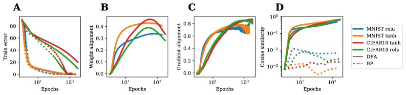
(a) No label corruption

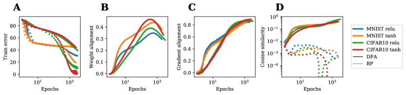
(b) 50% label corruption

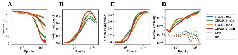
(c) 90% label corruption

Figure 11: Effect of label corruption on training observables. A: Training error. B and C: Weight and gradient alignment, as defined in the main text. D: Cosine similarity of the weight during training.

E.3 Experiment on the structure of targets

We trained a 3-layer linear MLP of width 100 for 1000 epochs on the synthetic dataset described in the main text, containing $10^{4}$ examples. We used the same hyperparameters as for the experiment on nonlinear networks. We choose 5 values for $\alpha$ and $\beta$: 0.2, 0.4, 0.6, 0.8 and 1.

In Fig. 12, we show the dynamics of weight alignment for both ReLU and Tanh activations. We again see the Align-then-Memorise process distinctly. Notice that decreasing $\alpha$ and $\beta$ hampers both the mamixmal weight alignment (at the end of the alignment phase) and the final weight alignment (at the end of the memorisation phase).

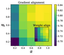
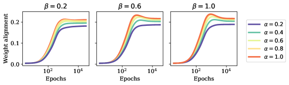
(a) ReLU

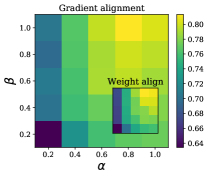
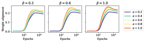
(b) Tanh

Figure 12: WA is hampered when the output dimensions are correlated ($\beta<1$) or of different variances ($\alpha<1$).

References

- Advani et al. (2020) Advani, M. S., Saxe, A. M., and Sompolinsky, H. High-dimensional dynamics of generalization error in neural networks. Neural Networks, 132:428 – 446, 2020.
- Aubin et al. (2018) Aubin, B., Maillard, A., Barbier, J., Krzakala, F., Macris, N., and Zdeborová, L. The committee machine: Computational to statistical gaps in learning a two-layers neural network. In Advances in Neural Information Processing Systems 31, pp. 3227–3238, 2018.
- Bahri et al. (2020) Bahri, Y., Kadmon, J., Pennington, J., Schoenholz, S., Sohl-Dickstein, J., and Ganguli, S. Statistical Mechanics of Deep Learning. Annual Review of Condensed Matter Physics, 11(1):501–528, 2020.
- Baity-Jesi et al. (2018) Baity-Jesi, M., Sagun, L., Geiger, M., Spigler, S., Arous, G., Cammarota, C., LeCun, Y., Wyart, M., and Biroli, G. Comparing Dynamics: Deep Neural Networks versus Glassy Systems. In Proceedings of the 35th International Conference on Machine Learning, 2018.
- Baldi & Hornik (1989) Baldi, P. and Hornik, K. Neural networks and principal component analysis: Learning from examples without local minima. Neural networks, 2(1):53–58, 1989.
- Bartunov et al. (2018) Bartunov, S., Santoro, A., Richards, B., Marris, L., Hinton, G. E., and Lillicrap, T. Assessing the scalability of biologically-motivated deep learning algorithms and architectures. In Advances in Neural Information Processing Systems, pp. 9368–9378, 2018.
- Biehl & Schwarze (1995) Biehl, M. and Schwarze, H. Learning by on-line gradient descent. J. Phys. A. Math. Gen., 28(3):643–656, 1995.
- Brutzkus & Globerson (2017) Brutzkus, A. and Globerson, A. Globally optimal gradient descent for a convnet with gaussian inputs. In Proceedings of the 34th International Conference on Machine Learning - Volume 70, ICML’17, pp. 605–614, 2017.
- Chizat & Bach (2018) Chizat, L. and Bach, F. On the global convergence of gradient descent for over-parameterized models using optimal transport. In Advances in Neural Information Processing Systems 31, pp. 3040–3050, 2018.
- Crafton et al. (2019) Crafton, B., Parihar, A., Gebhardt, E., and Raychowdhury, A. Direct feedback alignment with sparse connections for local learning. Frontiers in neuroscience, 13:525, 2019.
- Crick (1989) Crick, F. The recent excitement about neural networks. Nature, 337(6203):129–132, 1989.
- d’Ascoli et al. (2019) d’Ascoli, S., Sagun, L., Biroli, G., and Bruna, J. Finding the needle in the haystack with convolutions: on the benefits of architectural bias. In Advances in Neural Information Processing Systems, pp. 9334–9345, 2019.
- Du et al. (2018) Du, S., Lee, J., Tian, Y., Singh, A., and Poczos, B. Gradient descent learns one-hidden-layer CNN: Don’t be afraid of spurious local minima. In Proceedings of the 35th International Conference on Machine Learning, volume 80, pp. 1339–1348, 2018.
- Engel & Van den Broeck (2001) Engel, A. and Van den Broeck, C. Statistical mechanics of learning. Cambridge University Press, 2001.
- Frenkel et al. (2019) Frenkel, C., Lefebvre, M., and Bol, D. Learning without feedback: Direct random target projection as a feedback-alignment algorithm with layerwise feedforward training. 2019.
- Gabrié (2020) Gabrié, M. Mean-field inference methods for neural networks. Journal of Physics A: Mathematical and Theoretical, 53(22):223002, 2020.
- Gardner & Derrida (1989) Gardner, E. and Derrida, B. Three unfinished works on the optimal storage capacity of networks. Journal of Physics A: Mathematical and General, 22(12):1983–1994, 1989.
- Ghorbani et al. (2019) Ghorbani, B., Mei, S., Misiakiewicz, T., and Montanari, A. Limitations of lazy training of two-layers neural network. In Advances in Neural Information Processing Systems 32, pp. 9111–9121, 2019.
- Gilmer et al. (2017) Gilmer, J., Raffel, C., Schoenholz, S. S., Raghu, M., and Sohl-Dickstein, J. Explaining the learning dynamics of direct feedback alignment. In ICLR workshop track, 2017.
- Goldt et al. (2019) Goldt, S., Advani, M., Saxe, A., Krzakala, F., and Zdeborová, L. Dynamics of stochastic gradient descent for two-layer neural networks in the teacher-student setup. In Advances in Neural Information Processing Systems 32, 2019.
- Grossberg (1987) Grossberg, S. Competitive learning: From interactive activation to adaptive resonance. Cognitive science, 11(1):23–63, 1987.
- Han & Yoo (2019) Han, D. and Yoo, H.-j. Direct feedback alignment based convolutional neural network training for low-power online learning processor. In Proceedings of the IEEE International Conference on Computer Vision Workshops, 2019.
- Ji & Telgarsky (2019) Ji, Z. and Telgarsky, M. Gradient descent aligns the layers of deep linear networks. In International Conference on Learning Representations (ICLR), 2019.
- Kinzel & Ruján (1990) Kinzel, W. and Ruján, P. Improving a Network Generalization Ability by Selecting Examples. EPL (Europhysics Letters), 13(5):473–477, 1990.
- Krogh & Hertz (1992) Krogh, A. and Hertz, J. A. Generalization in a linear perceptron in the presence of noise. Journal of Physics A: Mathematical and General, 25(5):1135, 1992.
- Launay et al. (2019) Launay, J., Poli, I., and Krzakala, F. Principled training of neural networks with direct feedback alignment. arXiv:1906.04554, 2019.
- Launay et al. (2020) Launay, J., Poli, I., Boniface, F., and Krzakala, F. Direct feedback alignment scales to modern deep learning tasks and architectures. In Advances in neural information processing systems, 2020.
- Le Cun et al. (1991) Le Cun, Y., Kanter, I., and Solla, S. A. Eigenvalues of covariance matrices: Application to neural-network learning. Physical Review Letters, 66(18):2396, 1991.
- Liao et al. (2016) Liao, Q., Leibo, J. Z., and Poggio, T. How important is weight symmetry in backpropagation? In Proceedings of the Thirtieth AAAI Conference on Artificial Intelligence, pp. 1837–1844, 2016.
- Lillicrap et al. (2016) Lillicrap, T., Cownden, D., Tweed, D., and Akerman, C. Random synaptic feedback weights support error backpropagation for deep learning. Nature Communications, 7:1–10, 2016.
- Mei et al. (2018) Mei, S., Montanari, A., and Nguyen, P. A mean field view of the landscape of two-layer neural networks. Proceedings of the National Academy of Sciences, 115(33):E7665–E7671, 2018.
- Moskovitz et al. (2018) Moskovitz, T. H., Litwin-Kumar, A., and Abbott, L. Feedback alignment in deep convolutional networks. arXiv preprint arXiv:1812.06488, 2018.
- Nøkland (2016) Nøkland, A. Direct Feedback Alignment Provides Learning in Deep Neural Networks. In Advances in Neural Information Processing Systems 29, 2016.
- Rotskoff & Vanden-Eijnden (2018) Rotskoff, G. and Vanden-Eijnden, E. Parameters as interacting particles: long time convergence and asymptotic error scaling of neural networks. In Advances in Neural Information Processing Systems 31, pp. 7146–7155, 2018.
- Rumelhart et al. (1986) Rumelhart, D. E., Hinton, G. E., and Williams, R. J. Learning representations by back-propagating errors. Nature, 323(6088):533–536, 1986.
- Saad (2009) Saad, D. On-line learning in neural networks, volume 17. Cambridge University Press, 2009.
- Saad & Solla (1995a) Saad, D. and Solla, S. Exact Solution for On-Line Learning in Multilayer Neural Networks. Phys. Rev. Lett., 74(21):4337–4340, 1995a.
- Saad & Solla (1995b) Saad, D. and Solla, S. On-line learning in soft committee machines. Phys. Rev. E, 52(4):4225–4243, 1995b.
- Saxe et al. (2014) Saxe, A., McClelland, J., and Ganguli, S. Exact solutions to the nonlinear dynamics of learning in deep linear neural networks. In International Conference on Learning Representations (ICLR), 2014.
- Saxe et al. (2018) Saxe, A., Bansal, Y., Dapello, J., Advani, M., Kolchinsky, A., Tracey, B., and Cox, D. On the information bottleneck theory of deep learning. In ICLR, 2018.
- Seung et al. (1992) Seung, H. S., Sompolinsky, H., and Tishby, N. Statistical mechanics of learning from examples. Physical Review A, 45(8):6056–6091, 1992.
- Sirignano & Spiliopoulos (2019) Sirignano, J. and Spiliopoulos, K. Mean field analysis of neural networks: A central limit theorem. Stochastic Processes and their Applications, 2019.
- Soltanolkotabi et al. (2018) Soltanolkotabi, M., Javanmard, A., and Lee, J. Theoretical insights into the optimization landscape of over-parameterized shallow neural networks. IEEE Transactions on Information Theory, 65(2):742–769, 2018.
- Tian (2017) Tian, Y. An analytical formula of population gradient for two-layered relu network and its applications in convergence and critical point analysis. In Proceedings of the 34th International Conference on Machine Learning (ICML), pp. 3404–3413, 2017.
- Watkin et al. (1993) Watkin, T., Rau, A., and Biehl, M. The statistical mechanics of learning a rule. Reviews of Modern Physics, 65(2):499–556, 1993.
- Yoshida & Okada (2019) Yoshida, Y. and Okada, M. Data-dependence of plateau phenomenon in learning with neural network — statistical mechanical analysis. In Advances in Neural Information Processing Systems 32, pp. 1720–1728, 2019.
- Zdeborová & Krzakala (2016) Zdeborová, L. and Krzakala, F. Statistical physics of inference: thresholds and algorithms. Adv. Phys., 65(5):453–552, 2016.
- Zhong et al. (2017) Zhong, K., Song, Z., Jain, P., Bartlett, P., and Dhillon, I. Recovery guarantees for one-hidden-layer neural networks. In Proceedings of the 34th International Conference on Machine Learning-Volume 70, pp. 4140–4149, 2017.