Simulating Higher-Order Topological Insulators in Density Wave Insulators
Abstract
Since the discovery of the Harper-Hofstadter model, it has been known that condensed matter systems with periodic modulations can be promoted to non-trivial topological states with emergent gauge fields in higher dimensions. In this work, we develop a general procedure to compute the gauge fields in higher dimensions associated to low-dimensional systems with periodic (charge- and spin-) density wave modulations. We construct two-dimensional (2D) models with modulations that can be promoted to higher-order topological phases with and gauge fields in 3D. Corner modes in our 2D models can be pumped by adiabatic sliding of the phase of the modulation, yielding hinge modes in the promoted models. We also examine a 3D Weyl semimetal (WSM) gapped by charge-density wave (CDW) order, possessing quantum anomalous Hall (QAH) surface states. We show that this 3D system is equivalent to a 4D nodal line system gapped by a gauge field with a nonzero second Chern number. We explain the recently identified interpolation between inversion-symmetry protected phases of the 3D WSM gapped by CDWs using the corresponding 4D theory. Our results can extend the search for (higher-order) topological states in higher dimensions to density wave systems.
I Introduction
Topological crystalline phases in non-interacting, clean structures have attracted a great deal of recent theoretical and experimental attentionFu (2011); Hsieh et al. (2012); Ando and Fu (2015); Hughes et al. (2011); Turner et al. (2010, 2012). From the discovery of helical edge states in topological insulatorsKane and Mele (2005); Bernevig et al. (2006); König et al. (2007), to surface Dirac cones protected by time-reversal or crystal symmetriesFu et al. (2007); Xia et al. (2009); Hsieh et al. (2012); Wang et al. (2016), the experimental manifestations of band topology have come primarily through the exploration of surface states. The recent theoretical prediction of higher-order topological insulatorsSchindler et al. (2018a); Po et al. (2017); Khalaf (2018); Benalcazar et al. (2017) has triggered a wave of materials predictionsBradlyn et al. (2017); Vergniory et al. (2019); Zhang et al. (2019); Tang et al. (2019a); Xu et al. (2020) and experimental efforts to observe their predicted gapped surfaces but gapless corners (in 2D) or hinges (in 3D). At a theoretical level, topological band insulators can be classified by exploiting the constraints of symmetry, relating the topology of bands to the transformation properties of Bloch functions under crystal symmetriesKruthoff et al. (2017); Bradlyn et al. (2017); Po et al. (2017); Fu and Kane (2007); Po (2020); Cano and Bradlyn (2020); Elcoro et al. (2020); Watanabe et al. (2018); Zhang and Liu (2015); Bouhon et al. (2020). In the simplest cases, the symmetry eigenvalues of occupied electronic wavefunctions at different crystal momenta in the Brillouin zone can be used to deduce the absence of an exponentially localized, position space description of the occupied states, and hence the presence of non-trivial topology. Progress along these lines has led to a full, predictive classification of topological band structures both with and without time-reversal symmetry. Essential to these efforts is the presence of discrete translation symmetry, which ensures that localized electronic functions are identical in each unit cell, and hence allows the symmetry properties of the system to be described as a function of momentum.
At the same time, the interplay between topological bands and symmetry-breaking order has started to attract a great deal of attention. It has been argued theoretically that in topological systems with charge-density wave (CDW) order, the collective phason mode of the CDW may inherit topological properties from the Fermi sea, such as an induced axion coupling to electromagetic fieldsWang and Zhang (2013); You et al. (2016); Zyuzin and Burkov (2012); Zyuzin et al. (2012); Maciejko and Nandkishore (2014). Signatures of this axion coupling have been recently experimentally detected in (TaSe4)2IGooth et al. (2019); Shi et al. (2021). Additionally, the quantum anomalous Hall phase in the Dirac semimetal ZrTe5 can be understood as originating from a magnetic-field induced CDW transitionTang et al. (2019b); Qin et al. (2020); Song et al. (2017); Zhang and Shindou (2017). Because CDW order is in general incommensurate with the underlying lattice, a full understanding of the interplay between mean-field CDW order and band topology requires us to examine topology of incommensurately modulated electronic systems. Such a study would also yield insights into topology in artificially modulated photonicOzawa et al. (2019, 2016), metamaterialGrinberg et al. (2020), and cold-atomic lattice systemsAn et al. (2017), which have become a focus of recent research due to their tunability and experimental accessibility.
Naively, the breaking of translational and point group symmetries implied by incommensurate modulation would seem to prohibit the application of symmetry-based tools which have been so successful in identifying and classifying topological crystalline systems. However, it is often possible to view the single-particle dynamics in an incommensurately modulated system as describing the behavior of a particle in a larger number of dimensions, the phase offsets of the incommensurate modulations playing the role of momenta in the extra “synthetic” dimensions. The canonical example of this mapping is the 1D Harper (Aubry-André) model with incommensurate on-site potential. As was shown some time agoHofstadter (1976), the Hamiltonian for the Harper model is equivalent to the Hamiltonian for a 2D square-lattice system coupled to a background magnetic fieldKraus and Zilberberg (2012); Kraus et al. (2012). The phase of the on-site modulation plays the role of the momentum in the second, synthetic dimension, while the wavevector of the modulation plays the role of the magnetic flux per plaquette in the 2D lattice. Bands in the enhanced, 2D system can be characterized by a Chern number, which mandates the presence of gapless chiral modes at the edges of the system. Reducing back to 1D, these two-dimensional edge states manifest as boundary states of a 1D wire which appear and disappear as a function of the phase of modulation, thus realizing a Thouless pumpThouless (1983); Niu and Thouless (1984); Marra and Nitta (2020). Recent studies also show that certain generalization of the 1D Harper model allows for the investigation of higher-order topological phases Zeng et al. (2020).
In this work, we will extend the connection beyond 1D, to show how modulated systems in 2D and 3D can be related to topological crystalline phases in higher dimensions. We will first review a general method for representing a modulated system as a higher dimensional system coupled to a background gauge fieldRice and Mele (1982); Thouless (1983); Kraus et al. (2012); Kraus and Zilberberg (2012). For systems with negligible spin-orbit coupling and spin-independent modulation, the gauge field will be a magnetic field; for spin-dependent modulations we will show that there can also be induced gauge fields. We will exploit the fact that both and gauge fields with constant field strength preserve inversion symmetry to show that 2D modulated systems can realize higher-order chiral () and helical () topological phases in one extra synthetic dimension. We show how the hinge states of these synthetic higher-order topological insulators (HOTIs) manifest as corner modes in 2D, with energies that can be tuned by changing the phase of the modulation. Going further, we use the mapping to synthetic dimensions to bring order to the complex landscape of eigenstates of the modulated system, showing how the states can be interpreted as bulk and surface Landau level (LL) wavefunctions in synthetic dimensions. Finally, we also revisit a 3D minimal model for a Weyl semimetal (WSM) with (generally incommensurate) CDW orderWieder et al. (2020a), and show how it realizes a 4D nodal line semimetal gapped into a phase with a non-trivial second Chern number. We will verify our conclusions with a combination of exact numerical results and approximate low-energy analytic calculations. We will also exploit the fact that the phase of a (charge- or spin-) density wave (DW) order parameter can be shifted with an applied electromagnetic field, by exciting the (nominally gapless, but sometimes pinned) sliding modeGrüner (1988). This will allow us to make predictions about topological pumping of boundary states in modulated structures, driven by the sliding mode of the DW. In contrast to other recent proposals for topological pumping in synthetic dimensions, the coupling of the DW sliding mode to electromagnetic fields allows for tunability of synthetic dimensions in modulated structures. We will comment on potential experimental realizations in condensed matter, photonic, and cold-atom systems throughout. This work will enable new avenues for exploring higher-order topological phenomena which, with the exception of some promising results in BismuthHsu et al. (2019); Nayak et al. (2019); Schindler et al. (2018b), have not been unambiguously identified in crystalline electronic systems.
The rest of the paper is organized as follows. In Sec. II, we review how the Thouless pump in a 1D Rice-Mele [Su-Schrieffer-Heeger (SSH)] chain is realized by the sliding of a CDW, and we review its connection to topology by promoting the model to a 2D -flux lattice. In Sec. III we next develop a general method to compute the gauge fields that are coupled to a higher dimensional models promoted from a low-dimensional modulated system. In Secs. IV and V, we construct 2D modulated systems that can be promoted to 3D chiral and helical HOTIs coupled to and gauge fields, respectively. We demonstrate the pumping of corner modes by the sliding of DWs in these systems via numerical calculations of the energy spectra. We examine the properties of wave functions in these 2D modulated systems by constructing low energy theories coupled to gauge fields in 3D. We show how the evolution of bulk, edge, and corner states in 2D can be understood from the perspective of the low energy theory in 3D. In Sec. VI, we turn to a model for a 3D WSM gapped by a CDW. We show that this model can be promoted to a 4D nodal line system gapped by a gauge field. We derive the corresponding low energy theory in 4D, and use it to explain both the existence of QAH surface states and the interpolation between topologically distinct QAH phases at the two inversion-symmetric values of the CDW phase in this 3D system. Finally, in Sec. VII, we give an outlook as to how our work may extend the search of (higher-order) topological insulators in higher dimensions and enable simulations of gauge physics in higher dimensions. Some details of our models, further numerical results, and detailed derivations of the low energy theories are presented in the Supplementary Material (SM)SM .
Throughout this paper, we use units where , and where the electron has charge . Furthermore, the Einstein summation convention will not be used; whenever there is a summation over an index, we will write the summation explicitly.
II Review - Thouless Pump as Sliding Mode
In this section, we review the CDW picture of the Rice-Mele (SSH) modelRice and Mele (1982); Su et al. (1979), and the interpretation of the Thouless pumpThouless (1983) as a CDW sliding mode. Consider the following Hamiltonian for a 1D chain
| (1) |
where is the creation operator for an electron at site . The nearest-neighbor hopping and on-site potential are modulated with periodicity , and their relative strength is related to the phase of the modulation. We thus identify as the phase of this CDW modulation. In this paper, we use the terms ”CDW sliding phase” and ”phases of the mean-field CDW order parameter” interchangeably to refer to . For suitable choices of , and , the spectrum of this Hamiltonian is gapped for all . Focusing on the half-filled insulating ground state in this parameter regime, the occupied-band Wannier centersKohn (1959); Brouder et al. (2007); Marzari et al. (2012); Bradlyn et al. (2017); Shockley (1939) will be pumped by a length of one unit cell (two sites) as the phase adiabatically slides from to , leading to a quantized change of bulk polarizationXiao et al. (2010); Alexandradinata et al. (2014); Rice and Mele (1982); King-Smith and Vanderbilt (1993). This quantization has a topological origin: If we regard as a crystal momentum along a second, synthetic dimension which we call , Eq. (1) is equivalent to a 2D square lattice model with a -flux (equivalent to half flux quantum where electron has charge ) per plaquette, and with a fixed crystal momentum along . The quantized polarization change is then identified as the Chern numberThouless et al. (1982); Niu and Thouless (1984); Niu et al. (1985); Alexandradinata et al. (2014); Bernevig and Hughes (2013) of the occupied bands in 2D. We provide further details, including numerical verification of charge pumping, and the explicit construction of the dimensional promotion to 2D, in the SMSM .
We see from this example that promoting the dimension of a modulated system to a higher dimensional lattice coupled to gauge fields can help explain the topological origin of low-dimensional properties, including charge transport and boundary modes. A general method for dimensional promotion will thus be helpful in dealing with various topological modulated systems in more than 1D. In what follows, we will show that the dimensional promotion approach can be extended to higher dimensions, and to cases where the modulation is incommensurate with the underlying lattice periodicity.
III Dimensional Promotion Procedure
In this section, we will generalize the D-to-D dimensional promotion of the Rice-Mele chain to general dimensions. To begin, let us consider a -dimensional (D) electronic model on a cubic lattice with mutually incommensurate on-site modulationsRasing (1984); Kraus et al. (2012); Kraus and Zilberberg (2012); Kraus et al. (2013); Martin et al. (2017); Peng and Refael (2018), described by the Hamiltonian
| (2) |
Here both and are vectors in the D cubic lattice, and is the electron creation operator for an electron at position with a given set of spin and orbital degrees of freedom. We denote by the hopping matrix connecting position to , and by the matrix representing modulated on-site energy at position (), with matrix indices encoding the spin and orbital dependence of the hopping111throughout this work, we will use square brackets to denote matrices and matrix-valued functions. Note that hermiticity of the Hamiltonian requires that and . We further assume that with , where is the modulation wave vector and is the sliding phase associated with the modulation. For the cubic system with unit lattice vectors we are discussing here, each component , () of is defined within ; that is, each lies within the primitive Brillouin zone of the unmodulated system. Since each is a periodic function, they can be expanded in terms of Fourier series as
| (3) |
where is the matrix-valued Fourier component of . Note that due to hermiticity of the Hamiltonian.
To perform the enhancement of dimensions, we first insert the expansion Eq. (3) into the Hamiltonian Eq. (2). We then regard each as the crystal momentum along one of the additional synthetic dimensions. We then promote the D model to a D space by summing over (where denotes the -dimensional torus), which yields the Hamiltonian in D as
| (4) |
Each physically distinct configuration of can be recovered by restricting the Hamiltonian Eq. (4) to a single -point. Once we sum over , however, we can reinterpret the Hamiltonian in a D space. As we will see below, adiabatic pumping of the phases by an external field will allow us to explore dynamics in the full dimensional space.
To obtain the D model in position-space, we perform an inverse Fourier transform of , yielding
| (5) |
where and is the unit vector along the additional dimension, such that . Eq. (5) can be viewed as the Hamiltonian for a system on a D cubic lattice whose lattice sites are located at . The system is coupled to a continuous gauge field
| (6) |
through a Peierls substitutionPeierls (1933), explaining the appearance of the phase factors multiplying in Eq. (5). Note is a vector in the original D space.
As the vector potential in Eq. (6) is linear in position , the antisymmetric field strength is constant in space. In particular, Eq. (6) implies that the nonzero components of are given by
| (7) |
where and . Due to the antisymmetry of the field strength, with , is also nonzero and given by . Therefore the (nonzero) constant field strength is proportional to the magnitude of the modulation wave vectors.
This shows that that a D modulated system with phase offset is equivalent to the Bloch Hamiltonian (see Eq. (4)) of the promoted D lattice model with fixed crystal momenta , once we identify as . In practice, the modulation can be induced by a set of DW modulations. The phase offset is then regarded as the phason degrees of freedom, namely the phase of the mean-field DW order parameter. By applying electric fields that depin the DWs and make them slideGooth et al. (2019); Zak (1989); Grüner (1988), we may sample the whole spectrum of the D model. In particular, and as we will explore in subsequent sections, non-trivial topology in the D lattice model–which may support localized boundary states–will manifest in the response of the D model to adiabatic sliding of the DW phase mode(s). We emphasize here that in our dimensional promotion procedure for a DW system, there are no emergent electric fields in the promoted D space. The electric fields mentioned here are external and serve as a way to depin the DW in order to vary adiabatically. This allows for the sampling of the entire spectrum of the D model as a function of , namely the additional crystal momenta.
Before we move on to consider the band topology of promoted lattice models, let us make a few general comments about our dimensional promotion procedure. First, note that the dimensional promotion procedure places no constraints on the modulation vectors ; in particular, they need not be commensurate with the underlying lattice. In the case of incommensurate modulation, the dimensional promotion procedure allows us to write the D incommensurate model in terms of a periodic D model with an irrational flux per plaquette. We will see below how we can use this to explore the topology of systems with incommensurate modulation. We emphasize that the dimensional promotion procedure is independent of whether in the original D space the system is infinite or finite. When we promote the dimension of a D system to D space, the D system is inherently infinite along the additional dimensions, as it allows a Fourier transformation to obtain the Bloch Hamiltonian with fixed additional crystal momenta. From this viewpoint there are two ways to utilize the dimensional promotion procedure. If we promote the dimension of an infinite D system, we will obtain an infinite D system that allows us to discuss the non-trivial bulk topology in the promoted D space. If we instead promote the dimension of a finite D system, we will obtain a D system which is finite along the original dimensions and infinite in the additional dimensions. This allows us to compute the energy spectrum to examine whether there are boundary states protected by the non-trivial bulk topology in D space.
Second, although here we consider only dimensional promotion of a D cubic lattice model with only on-site modulations and all orbitals located at the lattice points labelled by to a D cubic lattice model, we may generalize our method to D models with modulations in both on-site and hopping matrix elements, together with non-orthogonal lattice vectors and arbitrary orbital positions. We show how to systematically promote the dimensions of such D models to D and compute the corresponding gauge fields in the SMSM . We also give several examples in the SMSM , including the dimensional promotion of: (1) the 1D Rice-Mele chain in Sec. II to a 2D square lattice with -flux, (2) 1D lattices with modulation in both on-site energies and hopping terms to 2D hexagonal lattices under a perpendicular magnetic field, and (3) 2D modulated systems with hexagonal lattice to 3D systems also with hexagonal lattices coupled to a gauge field. The gauge fields will take a slightly different form from Eq. (6) when we consider a system with non-orthogonal lattice vectors. However, the vector potentials will still be linear in , and hence will still produce constant field strengths . Furthermore, note that although we considered for simplicity models where the electrons were localized to the origin of each unit cell, this is not essential for the application of our formalism.
Third, we emphasize that no additional parameters are used in the above derivation. The hopping matrices connecting to and are given by and , respectively, in the D model. The phase corresponds to the crystal momentum along the additional dimensions. Further, the modulation wave vectors specify the strength of the gauge field in D, see Eq. (6). Notice that the on-site modulations only lead to hopping parallel to in D. If we also consider modulated hopping matrices in D, upon dimensional promotion we will get hopping along in DKraus and Zilberberg (2012); Petrides and Zilberberg (2020), which we show in the SMSM . Notice that the index is not summed over in . Recall also that and are vectors in the original D and additional D space, respectively. An example that demonstrates this is the 1D Rice-Mele modelRice and Mele (1982) in Sec. II. In the SMSM we promote Eq. (1) to a 2D lattice with -flux per plaquette in which the electrons can hop along (where and are in the original 1D and additional 1D space, respectively).
Next, our construction provides a way to compute the promoted D model and the gauge field to which it is coupled. As a gauge field breaks time-reversal-symmetry (TRS), this dimensional promotion procedure is suitable to investigate non-trivial topological phases in D space without TRS. Below we will also consider a dimensional promotion to D space with an gauge field, which preserves TRS and allows us to explore non-trivial topological phases protected by TRSKane and Mele (2005); Bernevig et al. (2006); Ryu et al. (2010); Kitaev (2009). In order to construct a low dimensional modulated model equivalent to a higher dimensional lattice coupled to an gauge field, we adopt a top-down approach. We will in Sec. V present a 2D modulated model which is obtained from a 3D model coupled to one gauge field with a fixed crystal momentum.
In the following sections, we explore various 2D and 3D modulated systems that admit a dimensional promotion to a higher dimensional topological phases coupled to either or gauge fields. We will show how an analysis of the higher-dimensional models can shed light on the eigenstates and boundary state dynamics of incommensurate DWs.
IV Chiral Higher-Order Topological Sliding Modes
In this section, we will show how the dimensional promotion procedure can be used to realize 3D chiral HOTIs in 2D density wave (DW) materials. We will first construct a Hamiltonian for an insulating 2D modulated system that is inversion-symmetric for special values of the DW sliding phase . Then, we will show how, after dimensional promotion, the Hamiltonian corresponds to a 3D inversion-symmetric chiral HOTI coupled to a gauge field. We will explore the connection between hinge states of the 3D system and corner states of the 2D system using a combination of numerical diagonalization and a 3D low-energy theory.
IV.1 Dimensionally Promoted Chiral Model
Consider the following 2D Hamiltonian for electrons on a square-lattice, with one modulated on-site potential :
| (8) | ||||
where the unmodulated hoppings and on-site energies are
| (9) | |||
| (10) |
We use to denote the unit vector along the () direction. The Pauli matrices and denote respectively orbital (for example and orbitals) and spin degrees of freedom. This Hamiltonian is inversion-symmetric, with inversion symmetry represented by . Furthermore, when the model is also time-reversal (TR) symmetric, with the TR operator represented as (where is the complex conjugation operator).
We assume that both orbital degrees of freedom are located at the lattice sites. The hopping matrices , and give rise to, at low energy, four-component massive Dirac fermions, allowing us to access various topological phasesRyu et al. (2010); Haldane (1988); Bernevig and Hughes (2013). Physically, we can interpret as the on-site energy difference for different orbitals, and as a ferromagnetic potential which splits the spin degeneracy of bandsWieder and Bernevig (2018). The modulated on-site potential, which can arise from a density wave modulation, is
| (11) |
where , is the modulation wave vector in 2D, is the lattice position, and is the sliding phase. The first term in Eq. (11) modulates the mass in Eq. (10), while the second modulation denotes an on-site spin-orbit coupling between and orbitals. Note that the modulation is a TR-even charge ordering, while is a TR-odd spin ordering. To see this, note that TR maps and . In addition, the modulations and are both inversion-symmetric when , .
Denoting the third, synthetic dimension as and identifying as the corresponding crystal momentum , we may use our general procedure in Sec. III to promote this 2D modulated system to a 3D lattice model. We first expand the modulations in terms of Fourier series as
| (12) | |||
| (13) |
According to Eqs. (3) and (5), the hopping along can be identified with the terms associated with in Eqs. (12) (13). Therefore, the hopping along in the promoted 3D space reads
| (14) |
From Eq. (6) we can also identify the vector potential in the promoted 3D space as
| (15) |
where . Therefore, we have that the lattice Hamiltonian in the promoted 3D space is given by
| (16) |
where the vector potential Eq. (6) is coupled to the system through a Peierls substitutionPeierls (1933), and , , and are given by Eqs. (9) and (10), respectively. Hereafter, we will set for simplicity. If we Fourier transform Eq. (16) along and regard (the wavenumber along ) as the sliding phase , we can obtain the 2D modulated system in Eq. (8).
We will now use Eq. (16) to analyze the topological properties of the higher-dimensional model, in order to infer the properties of the low-dimensional modulated system. This approach can also be employed in other low-dimensional modulated systems provided the corresponding higher-dimensional models are constructed. For and , Eq. (16) describes a TR and inversion-symmetric insulator whose inversion operation is represented by (note that inversion symmetry acts to flip the sign on the synthetic momentum ). We can employ the theory of symmetry-based indicators of band topology Khalaf et al. (2018); Po et al. (2017); Song et al. (2018); Xu et al. (2020); Elcoro et al. (2020); Wang et al. (2019); Wieder et al. (2020a); Kruthoff et al. (2017) to compute the indicator
| (17) |
where [] is the number of positive[negative] parity eigenvalues in the valence band at the time-reversal invariant momentum (TRIM) . We find that for , , , , the symmetry-based indicator is given by , , and , respectively. The regimes where give a strong TRS-invariant topological insulator (TI). For non-zero which breaks TRS but does not induce additional band inversions, the magnetic symmetry-based indicator Xu et al. (2020); Bradlyn et al. (2017); Elcoro et al. (2020); Po et al. (2017); Watanabe et al. (2018); Khalaf (2018); Wieder and Bernevig (2018); Zhang and Liu (2015); Bouhon et al. (2020); Yu et al. (2020a); Kim et al. (2019); Takahashi et al. (2020); Wieder et al. (2020a) is given by
| (18) |
such that for , , we have , and . The corresponding weak indices are all necessarily trivial. Therefore, for with , the system described by Eq. (16) gives a strong TI with and a chiral HOTI (axion insulator)Elcoro et al. (2020) with , where the gapless surface states of the strong TI are gapped by the inversion-preserving ferromagnetic potential . Therefore, Eq. (16) with describes an inversion-symmetric chiral HOTIPozo et al. (2019) coupled via a Peierls substitution to a 3D gauge field given by the in Eq. (6). This produces a constant magnetic field
| (19) |
which preserves the inversion symmetry represented by in 3D, up to a gauge transformation (see SMSM ). Therefore, for a suitable choice of parameters, as long as the gauge field does not close the bulk gap in 3D, the insulating ground state will be in the same inversion symmetry-protected non-trivial chiral HOTI phase. This implies that our model should exhibit the characteristic boundary modes of a chiral HOTI in 3D. In particular, our promoted model will support odd numbers of sample-encircling chiral hinge modes in rod geometries which respect inversion symmetry Pozo et al. (2019); Wieder and Bernevig (2018); Wieder et al. (2020a).
IV.2 Corner states
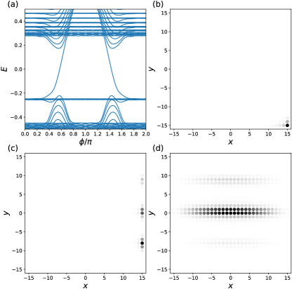
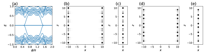
Recalling that in our case the direction is conjugate to the phase of the sliding mode (regarded as the crystal momentum ), it is natural for us to consider inversion-symmetric rod geometries which are finite in the and directions, and infinite in the direction. In our 2D system, this corresponds to considering the properties of a finite system as a function of the phase . We can thus compute the energy spectrum of our 2D system in an open geometry with size as a function of to obtain the energy dispersion along in the promoted model. In the following, we call this kind of calculation the -sliding spectrum, since the variation of can be obtained by electromagnetically exciting the sliding mode of the underlying DW. Fig. 1 (a) shows the -sliding spectrum of Eq. (8) with parameters , , , Pozo et al. (2019), and , where is comparable with the experimental CDW wave vectors in (TaSe4)2IShi et al. (2021) and is incommensurate with the underlying 2D square lattice in Eq. (8). The system size is . As we can see the spectrum contains modes which, as a function of , traverse the bulk spectral gap. Examining the wave functions of these “gap-crossing modes,” we see that they are localized to the corners of our D sample, as shown in Fig. 1 (b). The gap-crossing modes with opposite slopes correspond to states at inversion-related corners; in our example one mode is localized at the corner (Fig. 1 (b)) and the other at where . If we start in a half-filled insulating ground state (with Fermi level ), then as slides from to , we realize charge pumping as one corner mode merges into the occupied-state subspace while the inversion-related counterpart flows into the unoccupied state subspace. The ground states at the two inversion-symmetric values differ in electron number by , demonstrating a ”filling anomaly”Benalcazar et al. (2018); Wieder et al. (2020b). Because these corner modes originate as hinge modes in the D dimensionally promoted system (where, recall, is the momentum ), their existence is mandated by the non-trivial higher-order topology of the model Eq. (16).
By analyzing the low energy theory of the 3D hinge modes, we will now derive the dynamics of the 2D corner modes as a function of . In 3D, the corresponding low energy 1D hinge HamiltonianHasan and Kane (2010); Khalaf et al. (2018); Schindler et al. (2018a) with a chiral mode as a function of is given by
| (20) |
We have assumed that for the hinge along at position there is only one chiral mode with Fermi velocity where . We have introduced to denote whether the chiral mode has positive or negative velocity. Following our dimensional promotion procedure, Eq. (20) is then minimally coupled to a gauge field in Eq. (15) through the Peierls substitution , where and are fixed.
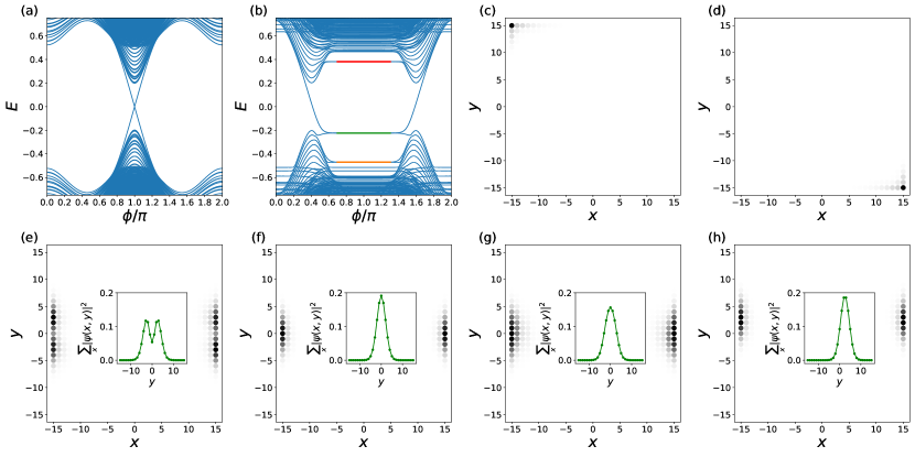
To map Eq. (20) in 3D to the corner mode dispersion in 2D, it is helpful to first compute the -sliding spectrum for Eq. (8) with , as shown in Fig. 2 (a). If we identify as in the hinge theory (modulo a constant offset that we will fix later), Fig. 2 (a) is the -directed rod band structure for Eq. (16) without coupling to any vector potential. As we can see, there are linear dispersing hinge modes spanning the bulk gap, which cross each other at . This will be used below in Eq. (21) to complete the mapping from Eq. (20) to 2D. Fig. 2 (a) will also serve as a reference calculation when we examine the response of the -sliding spectrum as we increase the magnitude of , which will confirm our low energy analysis.
We now use Eq. (20) to construct a low energy description of the corner modes in Fig. 1 (a) for Eq. (8). Upon projecting from 3D to 2D, the fixed hinge mode position becomes the fixed corner mode position , and the hinge modes become corner modes. Since the gap-crossing modes in the system shown in Fig. 2 (a) intersect at , we replace in the hinge theory by . Thus, we obtain an effective low energy description of the corner modes as
| (21) |
We now verify Eq. (21) by numerically computing the -sliding spectrum shown in Fig. 2 (b) with same parameters as Fig. 1 (a) but with changed to . This small value of gives a smooth modulation–and hence a low flux per plaquette in the dimensionally-promoted model–and is thus a suitable platform to examine the low energy theory with minimal coupling. We observe gap-crossing modes with negative and positive slopes corresponding to corner modes at and where , respectively. These are shown in Figs. 2 (c) and (d) at and , respectively. Using Eq. (21), we have the low energy descriptions for these two corner modes governed by the Hamiltonians
| (22) | |||
| (23) |
where we have used . Thus, if we ramp up from to some non-zero value, we expect to see the corner mode dispersion shift along the -axis. This is demonstrated in Fig. 2 (b), which is to be compared with Fig. 2 (a). In fact, a careful examination of Figs. 2 (a) and (b) shows that the dispersions of the two corner modes shift in opposite directions as a function of , as indicated in Eq. (22) and Eq. (23), with the shift given by for and . We thus see that the corner mode dispersion in Fig. 2 (b) can be explained by Eq. (21). This demonstrates the origin of the corner modes in the 2D modulated system as higher dimensional hinge modes minimally coupled to a gauge field. If we consider larger , such as in Fig. 1 where we have , then the shift of the corner mode dispersion is predicted to be . This lies outside the first Brillouin zone and needs to be folded back into the range . This occurs because, in passing from low energy continuum theory to a lattice model, the periodicity of –which in the promoted dimension is the continuous wavenumber –is restored. Additionally, note that Eq. (21) implies that we may tune the range of where the corner mode energies emerge from the bulk continuum by varying the periodicity of the modulation . As shown in Eq. (15) and Eq. (19), tuning is equivalent to changing the direction and strength of the gauge field and the corresponding magnetic field in 3D.
IV.3 Edge states
Having accounted for the low energy description of the corner modes, we observe that in Fig. 1 (a), there are additional modes with flat dispersion. These non-dispersing modes describe states confined either to the bulk or edge of the system, as shown in Figs. 1 (c) and (d). We now use low energy theories to demonstrate that these states originate from the Landau quantization of the surface and bulk electrons in the promoted 3D chiral HOTI. We will revisit Figs. 1 (c) and (d) after we complete the low energy theory analysis using relatively small .
We start with the edge-confined modes. Since a chiral HOTI can be obtained by gapping out the surface of a 3D inversion and TR-symmetric TI with a TR-breaking mass term, the generic surface theory readsKhalaf et al. (2018); Wieder and Bernevig (2018); Varnava and Vanderbilt (2018)
| (24) |
where are Pauli matrices that act in the basis of low-energy surface states and which capture their spin and orbital texture, is the momentum operator, and is the surface normal vector. The time-reversal operator in this surface theory is given by such that . The momentum dependent term describes a helical surface Dirac cone, while is the TR-breaking mass term. As shown in Eq. (19), if , which is the case we consider in Fig. 1 and Fig. 2, we have that is parallel to . We then consider a surface theory on the -plane coupled to a perpendicular magnetic field generated by a Landau-gauge gauge field . The corresponding surface Hamiltonian with the gauge field reads where we have made a Peierls substitution such that , and we have assumed that both and are positive. To facilitate the derivation, we perform a basis transformation through a radian spin rotation along the axis such that . The transformed Hamiltonian then reads
| (25) |
Fourier transforming Eq. (25) to replace by the wavenumber , and defining a -dependent ladder operator
| (26) |
where , we can rewrite Eq. (25) as
| (27) |
We can solve for the eigenstates and energy eigenvalues of Eq. (27) to find
| (28) |
Here is a non-negative integer labelling the Landau levels (LLs), and is the simple harmonic oscillator (SHO) eigenstate localized along defined by the in Eq. (26). Notice that the energies , and of these LLs shown in Eq. (28) are all independent of . As before, we now construct the low energy description of the edge-confined modes in the 2D modulated system from the above low energy surface theory in Eq. (25). We identify in the surface theory as , since we have flat bands as a function of in our 2D modulated system. We also identify with since in our examples of Fig. 1 (a) and Fig. 2 (b), we have and the corresponding vector potential is . When we project down to the 2D model, the surface electrons correspond to states confined in the left and right edges, as shown in Fig. 1 (c) and Fig. 2 (e)–(h). We again use to demonstrate the low energy theory.
We now remark on the implications of our low-energy analysis. First, the spectrum in Eq. (28) breaks particle-hole symmetry as there is a energy eigenvalue but no energy eigenvalue. This can be observed in Fig. 2 (b), where there are no flat bands of edge-confined modes around , which corresponds to . We thus identify the flat bands in Fig. 2 (b) marked by red, green and orange as , and in Eq. (28).
Second, from Eq. (28), the probability distributions for the states and are given by
| (29) | |||
| (30) |
up to a normalization factor, where is the eigenstate of an SHO localized along . Notice that we have indicated the explicit -dependence on since the cyclotron frequency and the localization of the wave function depend on the strength of magnetic field. This implies that has a pure Gaussian distribution. Furthermore, we expect that is more characteristic of an SHO first excited state than since , as we have assumed both and are positive. Figs. 2 (e)–(g) show the 2D wave function probability distributions at for edge confined modes in different LLs in our lattice model, together with the insets showing the integrated wave function probability over all -coordinates. While both Figs. 2 (e) and (g) corresponds to LL, the former is at the negative energy branch and the latter is at the positive energy branch. Therefore Fig. 2 (e) shows split peaks characteristic of the SHO first excited state, more so than Fig. 2 (g). In contrast, Fig. 2 (f), corresponding to the LL wave function, shows the Gaussian probability distribution characteristic of the SHO ground state. We see that the qualitative properties of the wave functions are all consistent with the low energy surface theory.
Third, the definition of the ladder operator in Eq. (26) implies that the center of the wave functions will be shifted by from . Identifying in the low energy theory as and as , we deduce that the distance that the edge-confined mode gets shifted along in the lattice model will be . Notice that the edge-confined mode in Fig. 2 (h) at () is shifted by lattice constants along comparing with Fig. 2 (f), which is at (). This is consistent with our prediction, as will be when and .
Fourth, although Eq. (28) predicts non-degenerate energy levels for a single surface with a perpendicular magnetic field, in Fig. 1 (a) the flat band corresponding to the level is highly degenerate. This is due to zone-folding effects, similar to what we observed for the corner mode dispersion in Fig. 1 (a). As the gap-crossing modes are shifted outside , they get folded back to together with the flat bands connected to them. Up to the degeneracy due to zone folding, the universal feature is that the edge-confined modes appearing in our 2D chiral DW system originate from the projection of surface electrons in a chiral HOTI with Landau quantization.
Before moving on, let us remark on the robustness of our low-energy predictions to perturbations of the model. If we consider a more complicated modulated system with, for example, long-range and anisotropic hopping terms together with other on-site potentials, as long as the promoted 3D system still preserves inversion symmetry and the gap is not closed, the 3D system will still be in the same chiral HOTI phase. However, the low energy theories that we have constructed might be modified. For example, the low energy theory at the surfaces, which we model with Eq. (25), may be modified as
| (31) |
Differences between and can lead to an anisotropic gapped Dirac cone. A nonzero induces unequal masses in different subspace of which can shift the entire energy spectrum. represents higher-order terms in the low energy theory which might cause nonlinearity in the band dispersion in Eq. (31) without minimal coupling. By the same reasoning, we might also have non-linear hinge mode energies with a quadratic momentum correction in Eq. (20). All of these additional terms will change the energetic feature of the system, such as energy spectra, Fermi velocities, together with the detailed form of the wave functions, which will be inevitably different from Eq. (28). Nevertheless, the following features are universal: (1) There will be electrons confined to the surface that undergo Landau quantization, and therefore there will be states that are confined along some directions. Upon projecting down to the 2D modulated system, we will still obtain edge-confined modes. (2) There will be (non-)linear hinge mode dispersion that will be shifted along due to the minimal coupling. Therefore the statement that we can tune the range of where the gap-crossing corner modes appear by tuning the magnitude of the modulation wave vectors, will still hold. We use the low energy theories Eq. (20) and Eq. (25) since these allow us to uncover the relation between the states in the promoted dimension and those in the original low dimensional modulated system in an analytically tractable way.
IV.4 Bulk states
The above analysis on corner- and edge-confined modes shows that the corresponding higher dimensional description of our modulated system is a 3D chiral HOTI minimally coupled to a gauge field. To complete our analysis, we will now focus on the bulk states. As expected, the low energy description of the bulk-confined modes, shown in Fig. 1 (d), will correspond to the low energy theory of bulk electrons in a 3D chiral HOTI minimally coupled to a gauge field. We start with the Bloch Hamiltonian of the promoted 3D chiral HOTI (Eq. (16) with ) expanded around the pointPozo et al. (2019),
| (32) |
We have defined several parameters to make Eq. (32) compact for later convenience, and introduced where corresponding to the ferromagnetic potential in Eq. (10). We now couple this to , which is equivalent to Eq. (15) with . This can be done via the minimal substitution . Fourier transforming along and to replace and by wavenumbers and , and defining the -dependent ladder operator as
| (33) |
we can rewrite Eq. (32) coupled to in terms of and as
| (34) |
We have numerically shown in SMSM that the effective theory in Eq. (34) captures several properties of the flat bulk bands in Fig. 2 (b) with relatively small , such as energy asymmetry with respect to and the confinement direction of the bulk states due to Landau quantization.
From the above analysis on corner-, edge-, and bulk-confined modes, we conclude that we can characterize this topological 2D modulated system with chiral sliding modes in terms of a 3D chiral HOTI coupled to a gauge field. In addition, such 2D modulated systems provide a platform to examine the properties of a 3D chiral HOTI, by sliding the DW order parameter .
V Helical Higher-Order Sliding Modes and Gauge Fields
Next, we will generalize our formalism to time-reversal invariant spinful systems. In doing so, we will see that incommensurate modulations induce coupling to gauge fields in the dimensionally promoted models. gauge fields can be used to represent spin-orbit couplingLi (2015), which is ubiquitous in topological states of matter. For example, gauge fields in 3D and 4D generates LLs that give rise to 3D TIs and 4D QHEsLi et al. (2013); Zhang and Hu (2001). A non-Abelian Peierls phase in 2D and 3D lattices can also lead to 2D and 3D TIsGoldman et al. (2010); Li (2015). In addition, in response to a bulk gauge flux insertion, a 2D TI can bind various quasi-particle excitations such as spinons, holons and chargeonsQi and Zhang (2008). In this section, we present a 2D modulated system that allows us to simulate a 3D helical HOTI coupled to an gauge field.
V.1 Dimensionally Promoted Helical Model
We start by considering the following 2D Hamiltonian on a square lattice with one modulated on-site potential :
| (35) | ||||
where the unmodulated couplings are are
| (36) | |||
| (37) | |||
| (38) |
The matrices , and , are Pauli matrices and denote the orbital, sub-lattice and spin degrees of freedom, respectively. The hopping matrices and , together with the on-site potential respect both inversion and TR symmetries. The inversion and TR operations are represented by and , respectivelyWang et al. (2019). These hoppings give rise to low energy four-component Dirac fermions in each spin subspace, realizing a topological critical point. The modulated on-site energy is given by
| (39) | |||||
where , is the modulation wave vector in 2D, is the lattice position, and is the sliding phase. The first term in Eq. (39) modulates the mass in Eq. (38), which may represent unequal on-site energy for and orbitals, with forward () and backward () sliding phase in each spin subspaceGoldman et al. (2010); Mei et al. (2012). The second term in Eq. (39) describes a modulation of the on-site energy which mixes and orbitals with unequal strength for different sublattices. Similarly, we have forward and backward sliding phases in different spin subspaces for the second term. Since the modulation in Eq. (39) has opposite phase offsets in each spin subspace, it may be induced from spin-orbit coupled spin ordering. This modulation is TR- and inversion-symmetric only when , . Note, however, that the product of inversion and TR symmetry, which we will denote -symmetry, is preserved for all values of . If we denote the third, synthetic dimension as , this 2D model is equivalent to the inversion and TR symmetric 3D helical HOTI model of Ref. Wang et al., 2019, coupled to an gauge field given by
| (40) |
This matrix-valued produces a constant magnetic fieldEstienne et al. (2011) , determined from the field strengthEguchi et al. (1980) , and given by
| (41) |
This constant field strength preserves both inversion and TR symmetry in 3D, up to a spin-dependent gauge transformation (see SMSM ). Notice that Eq. (41) implies that the magnetic field in this example can be interpreted as a magnetic field with opposite sign for spin-up and spin-down electronsGoldman et al. (2010); Mei et al. (2012). We then expect that, for a suitable choice of parameters such that the gauge field does not close the bulk gap in 3D, the insulating ground-state will be in the same non-trivial helical HOTI phase as the model with Khalaf et al. (2018); Schindler et al. (2018a); Po et al. (2017). Therefore, in 3D, our promoted model will support an odd number of pairs of sample-encircling helical hinge modes respecting inversion and TR symmetriesKhalaf et al. (2018); Wang et al. (2019). Upon projected back to 2D, the helical hinge modes in 3D become -related pairs of corner modes at the same in the 2D modulated system. In the SMSM , we give the form of the 3D dimensionally-promoted model in position-space.
V.2 Calculation of the Spectrum
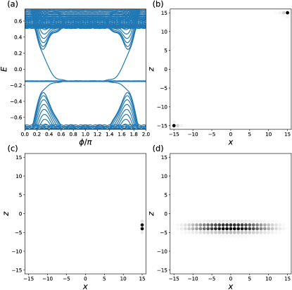
Let us now numerically verify these conclusions. Fig. 3 (a) shows the -sliding spectrum of Eq. (35) with parameters , , , , , , , Wang et al. (2019), and where Shi et al. (2021). The system size is . There are doubly-degenerate pairs of states which cross the gap as a function of , where the degeneracy is protected by -symmetry. We see from the wave functions that these are corner modes related by -symmetry, as shown in Fig. 3 (b) for the branch with negative slope around . In the other branch of doubly-degenerate gap-crossing states with positive slope, the corner modes are the inversion-symmetric counterpart (where recall that inversion symmetry leaves spin invariant) to those in Fig. 3 (b). Therefore, as slides from to , this model realizes a pumpFu and Kane (2006); Teo and Kane (2010) as one of the pairs of corner states will merge into the occupied state subspace (with Fermi level ) while the other pair will flow out. In our specific examples, the two states in each -related pair at the same are spin eigenstates and therefore in this case the pump is a spin pump; our conclusions, however, hold even when spin is not conserved.
As mentioned earlier, and in analogy with our chiral HOTI model, the corner modes here are equivalent to hinge modes along in 3D. The corresponding low energy theory for these corner modes is
| (42) |
where is the group velocity of the hinge modes in 3D. We use the Pauli matrices to denote the effective basis where in each subspace the states have opposite spin together with some orbital and sub-lattice textures. We have assumed without loss of generality that there is only one pair of helical hinge modes at the hinge along in the promoted 3D system. By denoting as , which is the crystal momentum along , we recognize Eq. (42) as the hinge mode dispersion in 3D minimally coupled to an gauge field described by Eq. (40). Similar to Sec. IV, as we vary –which is equivalent to changing the strength and (spatial) direction of the gauge field in Eqs. (40) and (41)–the dispersion of the spin-polarized corner modes will shift along the -axis. In the SMSM we present a complete low energy theory analysis for the corner modes with the same structure as Sec. IV.
In addition, we show in Figs. 3 (c) and (d) the probability density for the edge- and bulk-confined modes in the flat bands of Fig. 3 (a). Similar to the corner modes, these can be respectively understood in terms of 3D low energy surface and bulk theories minimally coupled to an gauge field, leading to an Landau quantizationLi et al. (2013); Li (2015). The relevant surface theory describes a time-reversed pair of Chern insulators. The relevant bulk theory is the expansion around of the promoted 3D helical HOTI HamiltonianWang et al. (2019). We provide further details in the SMSM . Together with the corner mode analysis, we see that this topological 2D modulated system with helical sliding modes can be characterized by a 3D lattice model coupled to an gauge field. In addition, we have shown how 2D modulated systems can provide a platform to examine gauge physics in higher dimensions, by sliding the phase of the DW order parameter.
VI Weyl-CDWs and 4D topological modes
As a final demonstration of our dimensional promotion formalism and its utility to investigating physics in more than 3D, we consider the mean-field state of a correlated inversion-symmetric 3D Weyl semimetal with CDW distortion (Weyl-CDW)Wieder et al. (2020a); Gooth et al. (2019); Shi et al. (2021); Wang and Zhang (2013); Sehayek et al. (2020); Cohn et al. (2020); Bobrow et al. (2020); Yu et al. (2020b). It has been shown that such a system can realize various topological phases. Depending on the phase of the CDW order parameter, the system can interpolate between quantum anomalous Hall (QAH) and obstructed QAH (oQAH) phaseWieder et al. (2020a). This is due to the mod axion angle difference for the system with and , in the thermodynamic limit. Physically, this leads to a Hall conductance difference
| (43) |
for a semi-infinite slab [see also Eq. (61) below, as well as Refs. Olsen et al., 2020; Varnava et al., 2020]. In this section, we analyze a minimal model of a 3D inversion-symmetric magnetic Weyl-CDW system, which admits a dimensional promotion to 4D with a gauge field. We will explain the origin of the background QAH response and the interpolation between QAH and oQAH phases using the corresponding 4D theory. In the following, we will denote a sample infinite along and with finite thickness along the direction as an -slab. Similarly, we will use the term -rod to denote a sample infinite along and finite along and with size .
VI.1 3D Weyl-CDW Model and Dimensional Promotion
To begin, we consider electrons on a 3D cubic-lattice with Hamiltonian . Here is a periodic tight-binding Hamiltonian given by
| (44) |
in position space. The corresponding Bloch Hamiltonian is
| (45) |
with . We take for the on-site modulation
| (46) |
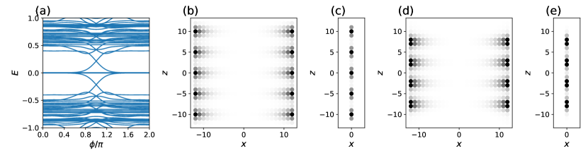
Here is the strength of the CDW modulation, is the magnitude of the modulation wave vector and is the phase of CDW order parameter. We again use to denote the Pauli matrices, which here index an orbital degree of freedom. The inversion and TR operation are represented by and , respectively (note that this is a model of spinless electrons). The Hamiltonian then describes a TR-breaking, inversion-symmetric magnetic Weyl semimetal (WSM) with Weyl nodes at , see Eq. (45)McCormick et al. (2017). The perturbation is the CDW modulation that couples these two Weyl nodes and opens a gap in the bulk spectrum Wieder et al. (2020a). Note that in this simple model, we have chosen the modulation wavevector to be exactly equal to the Weyl node separation vector for simplicity of analysis. Even though the bulk is gapped, the surface of this 3D Weyl-CDW is gapless, due to the presence of QAH surface states. In Fig. 4 (a) we show the -sliding spectrum for a -rod of at with size , , , and . This corresponds to a commensurate Weyl-CDW system. The mid-gap zero modes in Fig. 4 (a) correspond to the QAH surface states. In Fig. 4 (b) we show the probability distribution of the 10 zero modes at . Together with Wilson loop and Berry curvature calculation in the SMSM , we verify that the corresponding -slab with carries a slab Hall conductance . We can then identify the weak Chern numberQi et al. (2008); Kohmoto et al. (1992); Halperin (1987); Fu et al. (2007) of the 3D periodic system with unit cells (since ) as .
As in Sec. IV and V, we identify with the crystal momentum along a fourth, synthetic direction denoted by . Using the dimensional promotion procedure in Sec. III, we can promote to a 4D nodal line system coupled to a gauge field. In the SMSM we give the explicit form of the promoted model in 4D position space. The corresponding 4D nodal line system (with ) has a Bloch Hamiltonian
| (47) |
The spectrum of this Hamiltonian features nodal lines at defined by the implicit equation
| (48) |
According to Eq. (6), we then couple this Hamiltonian to a 4D gauge field given by
| (49) |
since in this system. This only produces non-zero field strength threading the plane,
| (50) |
where all other components of are zero. We are now in a position to reinterpret the existence of a background QAH response and QAH surface states when the bulk gap is opened due to the CDW. We will see how these features emerge from the low energy approximation for this 4D system minimally coupled to Eq. (49).
VI.2 Low Energy Theory Analysis
We start from the 4D Bloch Hamiltonian in Eq. (47). Expanding around , we have
| (51) |
The nodal line in this low energy theory is an ellipse in the - plane with , defined by
| (52) |
Replacing the 4D wave vector by the 4D momentum operator using the so-called envelope function approximationWinkler and Rössler (1993, 1994); Linder et al. (2009); König et al. (2008); Zhou et al. (2008); Qi and Zhang (2011); Hasan and Kane (2010); Bernevig et al. (2006), the Hamiltonian governing the low energy dynamics reads
| (53) |
Next, let us minimally couple Eq. (53) to a 4D gauge field via a Peierls substitution such that . Eq. (53) then becomes
| (54) |
where we have assumed that the particle carries charge. Fourier transforming along , and , we may replace , and by the corresponding wavenumbers , , , such that
| (55) |
Notice that the coefficient of in the final term in the Hamiltonian,
| (56) |
is an SHO Hamiltonian along which can be diagonalized as
| (57) |
Here is a non-negative integer and the eigenvalue of the number operator with
| (58) |
The quantum number is the 4D LL index. By restricting to a subspace of the full Hilbert space with fixed and , we see that the 4D low energy Hamiltonian Eq. (54) may be decomposed into a direct sum of 2D low energy Chern insulators (CIs) in -plane parameterized by and . The Hamiltonian for these 2D CIs is given by
| (59) |
where
| (60) |
Since we have restricted to the subspace with fixed and in Eq. (59), according to Eq. (56) the wave function along and will be SHO eigenstates centered at multiplied by a plane wave . Notice that the -dependence of Eq. (59) is due to the integer in Eq. (60) which is an eigenvalue of the number operator . Therefore, the eigenstates in the low energy approximation take the form of plane waves in , and Chern insulator eigenstates as a function of localized at different constant- planes for different . This provides a four-dimensional interpretation of the layer construction of the Weyl-CDW presented in Refs. Wieder et al., 2020a; Sehayek et al., 2020.
As in a 3D nodal ring system with a perpendicular magnetic field Li et al. (2018), Eq. (59) can yield a gapped 4D bulk spectrum provided that . This insulating ground state will then carry non-trivial topology inherited from the nodal line system, since in Eq. (59) we found that the gapped 4D continuum theory is composed of low energy 2D CIs. We then expect that there will be CI layers in the -plane of the corresponding 4D lattice model (see SMSM ). The CI layers will also be separated along by for a fixed , due to the periodicity of in the lattice model. In our current example this separation is since . Notice that is now interpreted as the crystal momentum along the dimension. To connect these observation in 4D back to the physical 3D Weyl-CDW system with Hamiltonian , we notice that each 3D Weyl-CDW system with a fixed corresponds to the 4D theory with a fixed . Focusing on the -slab with and thickness , in which , we show wavefunctions corresponding to the only layers of non-trivial CIs separated from each other by lattice constants along in Fig. 4 (c). Each of these CI layers carries Chern number and contributes one chiral edge mode along in the -rod, shown in Fig. 4 (b). In the SMSM we provide technical details on identifying the non-trivial CI layers using hybrid Wannier function, Berry phases and Berry curvature calculations for an -slab. We can thus regard the CDW-induced gap opening and the existence of background QAH response as the results of Landau quantization in the 4D nodal line system.
Next, we address the interpolation between the QAH phase at and the oQAH phase at using the 4D theory. Before we turn to the 4D low energy theory, we begin with the observation that in Fig. 4 (a), the number of mid-gap zero modes corresponding to QAH surface states decreases by as slides from to ; one state is lowered into the valence band, while one state is elevated to the conduction band. This is consistent with the change in Hall conductance Eq. (43), which is derived in the thermodynamic limit where the 2D slab thickness with infinitesimal but non-zero Wieder et al. (2020a). The ambiguity modulo in the change of Hall conductance is due to the axion angle , which is only well-defined mod , as shown below in Eq. (61). Taking with infinitesimal ensures that the only effect the CDW modulation has is to open the gap at the Weyl points without inverting bands at other high-symmetry points in the 3D Brillouin zone. We have also verified that our choice for the parameters in Fig. 4 (a) is adiabatically connected to this condition by increasing and decreasing . The slab Hall conductance of the -slab contains both an extensive contribution from the bulk QAH phase through the weak Chern number , and an intensive contribution from axion angle , which collectively givesVarnava and Vanderbilt (2018); Varnava et al. (2020)
| (61) |
where is the number of unit cells in the slab. In our examples for , will be given by . Recall also that as we slide from to , the bulk gap of the 3D Weyl-CDW system never closes, hence the is unchanged during the process. Putting this all together, we see that Eq. (43) implies that there is a mod change in the axion angle between and . To be more specific, in our current examples we have and . This quantized change of or can be explained again using the 4D low energy theory, as we now show.
Going back to the 4D low energy theory, Eq. (56) predicts that if we shift to , the corresponding CI layers described by the Hamiltonian in Eq. (59)–which are localized around –will be shifted in the direction by . Connecting this observation back to the physical 3D Weyl-CDW system, it implies that as we slide from to , all the CI layers will be shifted by ; for our choice of this gives a shift of . We demonstrate this numerically in Figs. 4 (d) and (e) which show the probability distribution of the QAH zero modes and the corresponding 4 non-trivial CI layers (with Chern number ) for . The physical interpretation of Eq. (43) is now clear: As we slide from to , the non-trivial CI layers will be shifted by unit cells, all in the same direction. Therefore, the bottom non-trivial CI layer at and depicted in Fig. 4 (c) will be shifted outside the finite sample and hence will not appear when . At , there will be only non-trivial CI layers remaining. This leads to a change in the Hall conductance by , as indicated by Eq. (43). Simultaneously, the number of QAH zero modes in the -rod decreases by when we slide from to . Physically, these two QAH zero modes are pushed toward the boundary of the system, due to the shifting of the bottom non-trivial CI layer. Therefore, their energies will be pushed toward the bulk continuum, leading to the inevitable appearance of gap-crossing bands as shown in Fig 4 (a). Numerically, we have observed that in all of our examples (Figs. 4 and 5), the zero modes in the band structure of the -rod only appear at . Therefore, as far as the zero modes are concerned, we can focus on the energy spectrum of the -rod at , as in Figs. 4 (a) and 5 (a). Analytically, this can be understood from the Hamiltonian of the low energy Chern insulator Eq. (59) for each and , which has zero energy edge modes only at Hasan and Kane (2010); Qi and Zhang (2011); Bernevig and Hughes (2013); Jackiw and Rebbi (1976).
To summarize, we have shown that the identity Eq. (43) can be regarded as a consequence of the Landau quantization of a 4D nodal line system in which the localization centers along of the states are directly related to . We then identified with the sliding phase through our dimensional promotion formalism in Sec. III. The change in conductance as a function of can thus be regarded as a physical manifestation of the Chern number polarization, which can alternatively be computed in terms of -localized hybrid Wannier centers Varnava et al. (2020); Zilberberg et al. (2018); Wieder et al. (2020a); Yu et al. (2020b); Olsen et al. (2020).
Having demonstrated the utility of our dimensional promotion formalism for a 3D Weyl-CDW system coupled to a commensurate CDW with , we next explore the case of incommensurate modulations which are prevalent in natureGrüner (1988). In particular, the experimentally intriguing Weyl-CDW (TaSe4)2I is incommensurateShi et al. (2021); Wang et al. (1983); Lee et al. (1985); Tournier-Colletta et al. (2013); Zhang et al. (2020); Shi et al. (2021). We still consider with , , . However, we now choose the modulation where is the golden ratio. For an -slab we choose and for -rod we choose . Since is an irrational number, the modulation is incommensurate with . Crucially though, we can use our dimensional promotion procedure regardless of whether or not the modulation is commensurate with the underlying lattice. The gauge field to which the 4D nodal line system is coupled still takes the form in Eq. (49). The main difference is that now, the 4D system has an irrational flux per plaquette in the plane. We have verified that for the -slab we have and , consistent with Eq. (61). We also show in Fig. 5 (a) the -sliding spectrum of the -rod at . We see that there are fewer QAH zero modes at than at . The 18 and 16 QAH zero modes for and are shown in Fig. 5 (c) and (e), respectively. We again identify 9 and 8 non-trivial states in the -slab at for and , and show their probability distributions in Fig. 5 (b) and (d), respectively. In the SMSM we present the details of the numerical methods for identifying non-trivial states in the -slab. The existence of non-zero QAH response and QAH zero modes can again be attributed to 4D Landau quantization which gaps the 4D nodal line system, yielding a topologically non-trivial insulating ground state. In particular, we also have mod . This can again be understood from the shifting of non-trivial CI layers. In this case, as slides from to , all the non-trivial CI layers will be shifted downward by lattice constants. The non-trivial CI layer at the bottom () of Fig. 5 (b) will be shifted outside the finite size system and thus the absolute value of slab Hall conductance will be changed by . Consequently, the number of QAH zero modes in the -rod at will be decreased by . Therefore, together with the examples in Sec. IV and Sec. V, we see that our dimensional promotion procedure provides a way to understand topological properties of systems with incommensurate modulations.
VI.3 Weyl-CDW and 4D Chern Number
We can also understand the topological properties of the Weyl-CDW model from the perspective of 4D response theory. Combining the field strength in Eq. (50) with our analysis of the Hall conductance above allows us to formulate a D field-theoretical description of the QAH response in a 3D Weyl-CDW system. The corresponding action is that of the D Chern-Simon theoryQi et al. (2008); Zhang and Hu (2001)
| (62) |
where is the second Chern number, is the electromagnetic gauge potential and is the Levi-Civita symbol in D. The Greek indices here are taken to run over all dimensions. Eq. (62) gives the electromagnetic response through
| (63) |
where is the current density along the direction. Since we have , an electric field along (implying ) will induce a Hall current density along through
| (64) |
Integrating this along the direction, we find then that, with non-zero , the Hall conductance is proportional to . This is consistent with Eq. (61) and the the recent calculationWieder et al. (2020a) showing that the Hall conductance of a 3D Weyl-CDW system is given by
| (65) |
where is the thickness of the -slab, is the CDW wave vector along , which in our specific model system is , and is the bulk axion angle computed from the inversion-symmetric unit cell. As we take the thermodynamic limit , the axion angle contribution to becomes negligible and thus can also be regarded as proportional to the magnitude of CDW wave vector, which is consistent with Eq. (64). Therefore, the field strength in Eq. (50) indeed allows a sensible construction of higher dimensional continuum theory.
To see concretely that the 3D Weyl-CDW system indeed emulates a 4D system with non-zero , we notice that for both examples in Fig. 4 and Fig. 5, the system can be deformed into a limit where we have layers of decoupled Chern insulators localized along . In the decoupled-layer limit, for the commensurate case, for example, , where we consider the single nontrivial band in each unit cell, this implies that , which is defined throughKraus et al. (2013); Zilberberg et al. (2018); Ozawa et al. (2016); Price et al. (2015); Qi et al. (2008)
| (66) |
becomes
| (67) |
in this limit, where is the Abelian Berry curvature in the - plane. For both examples in Fig. 4 and Fig. 5, we have identified the weak Chern number , implying that both systems have . In fact, for 3D Weyl-CDW system it have been shown that there will always be background QAH response in the planeWieder et al. (2020a), implying that in the limit of decoupled Chern insulators we have . Furthermore, as we shift the CDW sliding phase , which is equivalent to shifting the momentum , by , all the Chern insulating layers will be shifted by , implying a non-trivial Thouless charge pump along . Specifically, for Fig. 4 with , all the Chern insulating layers will be shifted by , which is equal to the unit cell length along , implying . The fact that the 3D Weyl-CDW system can be viewed as layers of Chern insulatorsWieder et al. (2020a) and the expression governing the charge pumping along as we vary by collectively predict a non-zero . Therefore, for a 3D Weyl-CDW system with QAH surface statesWieder et al. (2020a), the corresponding 4D theory is described by a (4+1)D Chern-Simon theory in Eq. (62) with non-zero . Furthermore, this result holds even as we deform away from the decoupled-layer limit, provided no energy gaps close. Thus the 3D Weyl-CDW system serves as a platform to study higher-dimensional topological field theories.
Let us conclude with two remarks. First, from the above analysis, we see that a 3D Weyl-CDW system with QAH surface states provides a platform to examine a 4D nodal line system gapped by a gauge field and carries non-zero second Chern number . Secondly, as opposed to Secs. IV and V where we have in higher dimensions a gapped topological phase coupled to or gauge fields, in the 4D model promoted from a 3D Weyl-CDW system it is precisely the coupling to a gauge field that opens up a bulk gap, inducing emergent CI layers, QAH surface states and non-zero .
VII Outlook
To conclude, we have shown in Secs. IV and V that higher-order topology in 3D can be probed in 2D DW systems. Furthermore, we showed in Sec. VI how 3D Weyl-CDW systems with background QAH response can be used to study 4D topology. The next and natural step is to identify 3D systems with modulations coexisting with hinge or corner modes. This will be a platform for studying 4–or even higher–dimensional higher-order topology. Our dimensional promotion procedure in Sec. III can also be used together with the topological classification based on crystalline symmetriesPo et al. (2017); Khalaf (2018); Chiu et al. (2016); Bradlyn et al. (2017) in the promoted dimensions, in order to explore topological crystalline phases in higher dimensions. With suitably chosen modulated systems, we may either study (1) how topological crystalline insulators diagnosed by symmetry-based indicatorsPo et al. (2017, 2018); Khalaf et al. (2018); Tang et al. (2019a); Po (2020); Watanabe et al. (2018) in the promoted dimensions respond to a background or gauge fields, or (2) how topological semimetalsArmitage et al. (2018) in the promoted dimensions can be gapped by background or gauge fields. With the dimensional promotion procedure, we may also extend our studies of topological materials to those with space groups beyond 3D, known as superspace groupsElcoro and Perez-Mato (1996); Janner and Janssen (1979); Janssen and Janner (2014); Bak and Janssen (1978); de Wolff et al. (1981). To extract the full information in higher dimension, a way to control the phase offset experimentally is needed, and currently applying electromagnetic fields to depin the (charge- or spin-)density waves is one practical approachGooth et al. (2019); Grüner (1988). In addition, since we can systematically compute the background continuous gauge field coupled to the dimensionally-promoted model, we can again use low dimensional modulated systems to study the low energy dynamics in higher dimensions, by minimally coupling the low energy theory to the known continuous gauge fields as in Sec. VI. As our dimensional promotion procedure can be carried out for both commensurate and incommensurate modulations, this approach can be used to study topological properties of system with quasi-periodic potentials Rasing (1984); Kraus et al. (2013); Zilberberg et al. (2018); Kraus and Zilberberg (2012); Kraus et al. (2012) where conventional band theory is not applicable. The general procedure will be to promote the dimension of these quasi-periodic systems and examine the response of possible topological phase in higher dimensions to a gauge field producing an irrational flux per plaquette. These techniques can be applied to analyze the DW phases in material systems of interest such as (TaSe4)2IGooth et al. (2019); Shi et al. (2021); Zhang et al. (2020); Tournier-Colletta et al. (2013) and ZrTe5Tang et al. (2019b); Qin et al. (2020); Song et al. (2017); Zhang and Shindou (2017). This can also lead to interesting studies on the higher-dimensional Hofstadter butterfly, complementing the recent studies of Refs. Lian et al., 2020; Herzog-Arbeitman et al., 2020. Another interesting direction is to introduce dynamics to the DW modulation. This can happen, for example, when the phase offsets acquire non-adiabatic time-dependence and become . Previous studies have focused on promoting the dimension of a periodically-driven system to a Floquet lattice, which under certain conditions can lead to topologically-protected quantized energy pump Martin et al. (2017); Peng and Refael (2018); Nathan et al. (2019). We expect that richer phenomena in higher-dimensional space can be investigated when the DW modulations are not only periodic in real-space but also (1) periodic in time or (2) have general time-dependence. Finally, we have shown in Sec. V the simplest case of how gauge field physics may be studied through a 2D modulated system. Recently, the spin-orbit-coupled Hofstadter models induced by non-Abelian gauge fields have also been studied both in 2DYang et al. (2020) and 3DLiu et al. (2020), where Dirac points with up to 16-fold degeneracy and various topological insulating states were found. We expect that 3D DW materials with different types of spin-orbit coupled modulations may enable simulation of various aspects of the physics of gauge fields in 4D or higher dimensions, including topological states and Hofstadter butterflies Li (2015); Yang et al. (2020); Liu et al. (2020). We hope that this work will lay the groundwork for the exciting future investigations mentioned above, and extend the search for exotic topological phases beyond 3D. In particular, there are many possible defects that one can imagine in a spin-orbit coupled density wave order parameter, each of which may correspond to a non-trivial response to gauge field defects in the higher-dimensional system.
Acknowledgements.
The authors would like to thank Y. Li and B. Wieder for fruitful discussions. This work was supported by the Alfred P. Sloan Foundation, and by the National Science Foundation under grant DMR-1945058. Numerical computations made use of the Illinois Campus Cluster, a computing resource that is operated by the Illinois Campus Cluster Program (ICCP) in conjunction with the National Center for Supercomputing Applications (NCSA) and which is supported by funds from the University of Illinois at Urbana-Champaign. Numerical calculations in this work employed the open-source PythTB packageCoh and Vanderbilt (2013).References
- Fu (2011) L. Fu, Phys. Rev. Lett. 106, 106802 (2011).
- Hsieh et al. (2012) T. H. Hsieh, H. Lin, J. Liu, W. Duan, A. Bansil, and L. Fu, Nature Communications 3, 932 (2012).
- Ando and Fu (2015) Y. Ando and L. Fu, Annu. Rev. Condens. Matter Phys. 6, 361 (2015).
- Hughes et al. (2011) T. L. Hughes, E. Prodan, and B. A. Bernevig, Phys. Rev. B 83, 245132 (2011).
- Turner et al. (2010) A. M. Turner, Y. Zhang, and A. Vishwanath, Phys. Rev. B 82, 241102 (2010).
- Turner et al. (2012) A. M. Turner, Y. Zhang, R. S. K. Mong, and A. Vishwanath, Phys. Rev. B 85, 165120 (2012).
- Kane and Mele (2005) C. L. Kane and E. J. Mele, Phys. Rev. Lett. 95, 226801 (2005).
- Bernevig et al. (2006) B. A. Bernevig, T. L. Hughes, and S.-C. Zhang, Science 314, 1757 (2006).
- König et al. (2007) M. König, S. Wiedmann, C. Brüne, A. Roth, H. Buhmann, L. W. Molenkamp, X.-L. Qi, and S.-C. Zhang, Science 318, 766 (2007).
- Fu et al. (2007) L. Fu, C. L. Kane, and E. J. Mele, Phys. Rev. Lett. 98, 106803 (2007).
- Xia et al. (2009) Y. Xia, D. Qian, D. Hsieh, L. Wray, A. Pal, H. Lin, A. Bansil, D. Grauer, Y. S. Hor, R. J. Cava, and M. Z. Hasan, Nature physics 5, 398 (2009).
- Wang et al. (2016) Z. Wang, A. Alexandradinata, R. J. Cava, and B. A. Bernevig, Nature 532, 189 (2016).
- Schindler et al. (2018a) F. Schindler, A. M. Cook, M. G. Vergniory, Z. Wang, S. S. P. Parkin, B. A. Bernevig, and T. Neupert, Science Advances 4 (2018a), 10.1126/sciadv.aat0346, http://advances.sciencemag.org/content/4/6/eaat0346.full.pdf .
- Po et al. (2017) H. C. Po, A. Vishwanath, and H. Watanabe, Nat. Comm. 8, 50 (2017).
- Khalaf (2018) E. Khalaf, Physical Review B 97, 205136 (2018).
- Benalcazar et al. (2017) W. A. Benalcazar, B. A. Bernevig, and T. L. Hughes, Science 357, 61 (2017).
- Bradlyn et al. (2017) B. Bradlyn, L. Elcoro, J. Cano, M. G. Vergniory, Z. Wang, C. Felser, M. I. Aroyo, and B. A. Bernevig, Nature 547, 298 (2017).
- Vergniory et al. (2019) M. Vergniory, L. Elcoro, C. Felser, B. Bernevig, and Z. Wang, Nature 566, 480 (2019).
- Zhang et al. (2019) T. Zhang, Y. Jiang, Z. Song, H. Huang, Y. He, Z. Fang, H. Weng, and C. Fang, Nature 566, 475 (2019).
- Tang et al. (2019a) F. Tang, H. C. Po, A. Vishwanath, and X. Wan, Nature Physics 15, 470 (2019a).
- Xu et al. (2020) Y. Xu, L. Elcoro, Z.-D. Song, B. J. Wieder, M. Vergniory, N. Regnault, Y. Chen, C. Felser, and B. A. Bernevig, Nature 586, 702 (2020).
- Kruthoff et al. (2017) J. Kruthoff, J. de Boer, J. van Wezel, C. L. Kane, and R.-J. Slager, Phys. Rev. X 7, 041069 (2017).
- Fu and Kane (2007) L. Fu and C. L. Kane, Phys. Rev. B 76, 045302 (2007).
- Po (2020) H. C. Po, Journal of Physics: Condensed Matter 32, 263001 (2020).
- Cano and Bradlyn (2020) J. Cano and B. Bradlyn, arXiv preprint arXiv:2006.04890 (2020).
- Elcoro et al. (2020) L. Elcoro, B. J. Wieder, Z. Song, Y. Xu, B. Bradlyn, and B. A. Bernevig, arXiv preprint arXiv:2010.00598 (2020).
- Watanabe et al. (2018) H. Watanabe, H. C. Po, and A. Vishwanath, Science advances 4, eaat8685 (2018).
- Zhang and Liu (2015) R.-X. Zhang and C.-X. Liu, Phys. Rev. B 91, 115317 (2015).
- Bouhon et al. (2020) A. Bouhon, G. F. Lange, and R.-J. Slager, arXiv e-prints , arXiv:2010.10536 (2020), arXiv:2010.10536 [cond-mat.mes-hall] .
- Wang and Zhang (2013) Z. Wang and S.-C. Zhang, Physical Review B 87, 161107 (2013).
- You et al. (2016) Y. You, G. Y. Cho, and T. L. Hughes, Physical Review B 94, 085102 (2016).
- Zyuzin and Burkov (2012) A. A. Zyuzin and A. A. Burkov, Phys. Rev. B 86, 115133 (2012).
- Zyuzin et al. (2012) A. Zyuzin, S. Wu, and A. Burkov, Physical Review B 85, 165110 (2012).
- Maciejko and Nandkishore (2014) J. Maciejko and R. Nandkishore, Physical Review B 90, 035126 (2014).
- Gooth et al. (2019) J. Gooth, B. Bradlyn, S. Honnali, C. Schindler, N. Kumar, J. Noky, Y. Qi, C. Shekhar, Y. Sun, Z. Wang, B. A. Bernevig, and C. Felser, Nature 575, 315 (2019).
- Shi et al. (2021) W. Shi, B. J. Wieder, H. Meyerheim, Y. Sun, Y. Zhang, Y. Li, L. Shen, Y. Qi, L. Yang, J. Jena, et al., Nature Physics 17, 381 (2021).
- Tang et al. (2019b) F. Tang, Y. Ren, P. Wang, R. Zhong, J. Schneeloch, S. A. Yang, K. Yang, P. A. Lee, G. Gu, Z. Qiao, et al., Nature 569, 537 (2019b).
- Qin et al. (2020) F. Qin, S. Li, Z. Du, C. Wang, H.-Z. Lu, and X. Xie, arXiv preprint arXiv:2003.02520 (2020).
- Song et al. (2017) Z. Song, Z. Fang, and X. Dai, Physical Review B 96, 235104 (2017).
- Zhang and Shindou (2017) X.-T. Zhang and R. Shindou, Physical Review B 95, 205108 (2017).
- Ozawa et al. (2019) T. Ozawa, H. M. Price, A. Amo, N. Goldman, M. Hafezi, L. Lu, M. C. Rechtsman, D. Schuster, J. Simon, O. Zilberberg, and I. Carusotto, Rev. Mod. Phys. 91, 015006 (2019).
- Ozawa et al. (2016) T. Ozawa, H. M. Price, N. Goldman, O. Zilberberg, and I. Carusotto, Physical Review A 93, 043827 (2016).
- Grinberg et al. (2020) I. H. Grinberg, M. Lin, C. Harris, W. A. Benalcazar, C. W. Peterson, T. L. Hughes, and G. Bahl, Nature communications 11, 1 (2020).
- An et al. (2017) F. A. An, E. J. Meier, and B. Gadway, Science Advances 3 (2017), 10.1126/sciadv.1602685, https://advances.sciencemag.org/content/3/4/e1602685.full.pdf .
- Hofstadter (1976) D. R. Hofstadter, Phys. Rev. B 14, 2239 (1976).
- Kraus and Zilberberg (2012) Y. E. Kraus and O. Zilberberg, Phys. Rev. Lett. 109, 116404 (2012).
- Kraus et al. (2012) Y. E. Kraus, Y. Lahini, Z. Ringel, M. Verbin, and O. Zilberberg, Phys. Rev. Lett. 109, 106402 (2012).
- Thouless (1983) D. J. Thouless, Phys. Rev. B 27, 6083 (1983).
- Niu and Thouless (1984) Q. Niu and D. Thouless, Journal of Physics A: Mathematical and General 17, 2453 (1984).
- Marra and Nitta (2020) P. Marra and M. Nitta, Phys. Rev. Research 2, 042035 (2020).
- Zeng et al. (2020) Q.-B. Zeng, Y.-B. Yang, and Y. Xu, Phys. Rev. B 101, 241104 (2020).
- Rice and Mele (1982) M. J. Rice and E. J. Mele, Phys. Rev. Lett. 49, 1455 (1982).
- Wieder et al. (2020a) B. J. Wieder, K.-S. Lin, and B. Bradlyn, Physical Review Research 2, 042010 (2020a).
- Grüner (1988) G. Grüner, Reviews of modern physics 60, 1129 (1988).
- Hsu et al. (2019) C.-H. Hsu, X. Zhou, T.-R. Chang, Q. Ma, N. Gedik, A. Bansil, S.-Y. Xu, H. Lin, and L. Fu, Proceedings of the National Academy of Sciences 116, 13255 (2019).
- Nayak et al. (2019) A. K. Nayak, J. Reiner, R. Queiroz, H. Fu, C. Shekhar, B. Yan, C. Felser, N. Avraham, and H. Beidenkopf, Science advances 5, eaax6996 (2019).
- Schindler et al. (2018b) F. Schindler, Z. Wang, M. G. Vergniory, A. M. Cook, A. Murani, S. Sengupta, A. Y. Kasumov, R. Deblock, S. Jeon, I. Drozdov, et al., Nature physics 14, 918 (2018b).
- (58) See Supplemental Material [url] for the description of general dimensional promotion method, additional examples of dimensional promotion and other numerical calculations, which includes Refs. Resta, 1994; Fidkowski et al., 2011; Yu et al., 2011; Alexandradinata and Bernevig, 2016.
- Su et al. (1979) W. P. Su, J. R. Schrieffer, and A. J. Heeger, Phys. Rev. Lett. 42, 1698 (1979).
- Kohn (1959) W. Kohn, Phys. Rev. 115, 809 (1959).
- Brouder et al. (2007) C. Brouder, G. Panati, M. Calandra, C. Mourougane, and N. Marzari, Phys. Rev. Lett. 98, 046402 (2007).
- Marzari et al. (2012) N. Marzari, A. A. Mostofi, J. R. Yates, I. Souza, and D. Vanderbilt, Rev. Mod. Phys. 84, 1419 (2012).
- Shockley (1939) W. Shockley, Physical review 56, 317 (1939).
- Xiao et al. (2010) D. Xiao, M.-C. Chang, and Q. Niu, Reviews of modern physics 82, 1959 (2010).
- Alexandradinata et al. (2014) A. Alexandradinata, X. Dai, and B. A. Bernevig, Phys. Rev. B 89, 155114 (2014).
- King-Smith and Vanderbilt (1993) R. D. King-Smith and D. Vanderbilt, Phys. Rev. B 47, 1651(R) (1993).
- Thouless et al. (1982) D. J. Thouless, M. Kohmoto, M. P. Nightingale, and M. den Nijs, Physical Review Letters 49, 405 (1982).
- Niu et al. (1985) Q. Niu, D. J. Thouless, and Y.-S. Wu, Physical Review B 31, 3372 (1985).
- Bernevig and Hughes (2013) B. A. Bernevig and T. L. Hughes, Topological Insulators and Topological Superconductors (Princeton University Press, Princeton, NJ, 2013).
- Rasing (1984) T. Rasing, Phys. Rev. Lett. 53, 388 (1984).
- Kraus et al. (2013) Y. E. Kraus, Z. Ringel, and O. Zilberberg, Phys. Rev. Lett. 111, 226401 (2013).
- Martin et al. (2017) I. Martin, G. Refael, and B. Halperin, Phys. Rev. X 7, 041008 (2017).
- Peng and Refael (2018) Y. Peng and G. Refael, Phys. Rev. B 97, 134303 (2018).
- Note (1) Throughout this work, we will use square brackets to denote matrices and matrix-valued functions.
- Peierls (1933) R. Peierls, Zeitschrift für Physik 80, 763 (1933).
- Zak (1989) J. Zak, Phys. Rev. Lett. 62, 2747 (1989).
- Petrides and Zilberberg (2020) I. Petrides and O. Zilberberg, Phys. Rev. Research 2, 022049 (2020).
- Ryu et al. (2010) S. Ryu, A. P. Schnyder, A. Furusaki, and A. W. Ludwig, New Journal of Physics 12, 065010 (2010).
- Kitaev (2009) A. Kitaev, in American Institute of Physics Conference Series, American Institute of Physics Conference Series, Vol. 1134, edited by V. Lebedev and M. Feigel’Man (2009) pp. 22–30, arXiv:0901.2686 [cond-mat.mes-hall] .
- Haldane (1988) F. D. M. Haldane, Phys. Rev. Lett. 61, 2015 (1988).
- Wieder and Bernevig (2018) B. J. Wieder and B. A. Bernevig, arXiv preprint arXiv:1810.02373 (2018).
- Khalaf et al. (2018) E. Khalaf, H. C. Po, A. Vishwanath, and H. Watanabe, Phys. Rev. X 8, 031070 (2018).
- Song et al. (2018) Z. Song, T. Zhang, Z. Fang, and C. Fang, Nat. Commun. 9, 3530 (2018).
- Wang et al. (2019) Z. Wang, B. J. Wieder, J. Li, B. Yan, and B. A. Bernevig, Phys. Rev. Lett. 123, 186401 (2019).
- Yu et al. (2020a) J. Yu, Z.-D. Song, and C.-X. Liu, Phys. Rev. Lett. 125, 036401 (2020a).
- Kim et al. (2019) H. Kim, K. Shiozaki, and S. Murakami, Phys. Rev. B 100, 165202 (2019).
- Takahashi et al. (2020) R. Takahashi, Y. Tanaka, and S. Murakami, Phys. Rev. Research 2, 013300 (2020).
- Pozo et al. (2019) O. Pozo, C. Repellin, and A. G. Grushin, Physical Review Letters 123, 247401 (2019).
- Benalcazar et al. (2018) W. A. Benalcazar, T. Li, and T. L. Hughes, arXiv preprint arXiv:1809.02142 (2018).
- Wieder et al. (2020b) B. J. Wieder, Z. Wang, J. Cano, X. Dai, L. M. Schoop, B. Bradlyn, and B. A. Bernevig, Nature communications 11, 1 (2020b).
- Hasan and Kane (2010) M. Z. Hasan and C. L. Kane, Reviews of modern physics 82, 3045 (2010).
- Varnava and Vanderbilt (2018) N. Varnava and D. Vanderbilt, Phys. Rev. B 98, 245117 (2018).
- Li (2015) Y. Li, Phys. Rev. B 91, 195133 (2015).
- Li et al. (2013) Y. Li, S.-C. Zhang, and C. Wu, Phys. Rev. Lett. 111, 186803 (2013).
- Zhang and Hu (2001) S.-C. Zhang and J. Hu, Science 294, 823 (2001).
- Goldman et al. (2010) N. Goldman, I. Satija, P. Nikolic, A. Bermudez, M. A. Martin-Delgado, M. Lewenstein, and I. B. Spielman, Phys. Rev. Lett. 105, 255302 (2010).
- Qi and Zhang (2008) X.-L. Qi and S.-C. Zhang, Phys. Rev. Lett. 101, 086802 (2008).
- Mei et al. (2012) F. Mei, S.-L. Zhu, Z.-M. Zhang, C. H. Oh, and N. Goldman, Phys. Rev. A 85, 013638 (2012).
- Estienne et al. (2011) B. Estienne, S. M. Haaker, and K. Schoutens, New Journal of Physics 13, 045012 (2011).
- Eguchi et al. (1980) T. Eguchi, P. B. Gilkey, and A. J. Hanson, Physics reports 66, 213 (1980).
- Fu and Kane (2006) L. Fu and C. L. Kane, Physical Review B 74, 195312 (2006).
- Teo and Kane (2010) J. C. Teo and C. L. Kane, Physical Review B 82, 115120 (2010).
- Sehayek et al. (2020) D. Sehayek, M. Thakurathi, and A. A. Burkov, arXiv e-prints , arXiv:2007.07256 (2020), arXiv:2007.07256 [cond-mat.str-el] .
- Cohn et al. (2020) I. A. Cohn, S. G. Zybtsev, A. P. Orlov, and S. V. Zaitsev-Zotov, arXiv e-prints , arXiv:2006.12288 (2020), arXiv:2006.12288 [cond-mat.mtrl-sci] .
- Bobrow et al. (2020) E. Bobrow, C. Sun, and Y. Li, Phys. Rev. Research 2, 012078 (2020).
- Yu et al. (2020b) J. Yu, B. J. Wieder, and C.-X. Liu, arXiv preprint arXiv:2008.10620 (2020b).
- Olsen et al. (2020) T. Olsen, T. Rauch, D. Vanderbilt, and I. Souza, Physical Review B 102, 035166 (2020).
- Varnava et al. (2020) N. Varnava, I. Souza, and D. Vanderbilt, Phys. Rev. B 101, 155130 (2020).
- McCormick et al. (2017) T. M. McCormick, I. Kimchi, and N. Trivedi, Physical Review B 95, 075133 (2017).
- Qi et al. (2008) X.-L. Qi, T. L. Hughes, and S.-C. Zhang, Physical Review B 78, 195424 (2008).
- Kohmoto et al. (1992) M. Kohmoto, B. I. Halperin, and Y.-S. Wu, Phys. Rev. B 45, 13488 (1992).
- Halperin (1987) B. I. Halperin, Japanese Journal of Applied Physics 26, 1913 (1987).
- Winkler and Rössler (1993) R. Winkler and U. Rössler, Phys. Rev. B 48, 8918 (1993).
- Winkler and Rössler (1994) R. Winkler and U. Rössler, Surface Science 305, 295 (1994).
- Linder et al. (2009) J. Linder, T. Yokoyama, and A. Sudbø, Phys. Rev. B 80, 205401 (2009).
- König et al. (2008) M. König, H. Buhmann, L. W. Molenkamp, T. Hughes, C.-X. Liu, X.-L. Qi, and S.-C. Zhang, Journal of the Physical Society of Japan 77, 031007 (2008), https://doi.org/10.1143/JPSJ.77.031007 .
- Zhou et al. (2008) B. Zhou, H.-Z. Lu, R.-L. Chu, S.-Q. Shen, and Q. Niu, Phys. Rev. Lett. 101, 246807 (2008).
- Qi and Zhang (2011) X.-L. Qi and S.-C. Zhang, Rev. Mod. Phys. 83, 1057 (2011).
- Li et al. (2018) C. Li, C. M. Wang, B. Wan, X. Wan, H.-Z. Lu, and X. C. Xie, Phys. Rev. Lett. 120, 146602 (2018).
- Jackiw and Rebbi (1976) R. Jackiw and C. Rebbi, Phys. Rev. D 13, 3398 (1976).
- Zilberberg et al. (2018) O. Zilberberg, S. Huang, J. Guglielmon, M. Wang, K. P. Chen, Y. E. Kraus, and M. C. Rechtsman, Nature 553, 59 (2018).
- Wang et al. (1983) Z. Z. Wang, M. Saint-Lager, P. Monceau, M. Renard, P. Gressier, A. Meerschaut, L. Guemas, and J. Rouxel, Solid state communications 46, 325 (1983).
- Lee et al. (1985) K.-B. Lee, D. Davidov, and A. Heeger, Solid state communications 54, 673 (1985).
- Tournier-Colletta et al. (2013) C. Tournier-Colletta, L. Moreschini, G. Autes, S. Moser, A. Crepaldi, H. Berger, A. Walter, K. S. Kim, A. Bostwick, P. Monceau, et al., Physical review letters 110, 236401 (2013).
- Zhang et al. (2020) Y. Zhang, L.-F. Lin, A. Moreo, S. Dong, and E. Dagotto, Physical Review B 101, 174106 (2020).
- Price et al. (2015) H. M. Price, O. Zilberberg, T. Ozawa, I. Carusotto, and N. Goldman, Phys. Rev. Lett. 115, 195303 (2015).
- Chiu et al. (2016) C.-K. Chiu, J. C. Y. Teo, A. P. Schnyder, and S. Ryu, Rev. Mod. Phys. 88, 035005 (2016).
- Po et al. (2018) H. C. Po, H. Watanabe, and A. Vishwanath, Phys. Rev. Lett. 121, 126402 (2018).
- Armitage et al. (2018) N. Armitage, E. Mele, and A. Vishwanath, Reviews of Modern Physics 90, 015001 (2018).
- Elcoro and Perez-Mato (1996) L. Elcoro and J. M. Perez-Mato, Phys. Rev. B 54, 12115 (1996).
- Janner and Janssen (1979) A. Janner and T. Janssen, Physica A: Statistical Mechanics and its Applications 99, 47 (1979).
- Janssen and Janner (2014) T. Janssen and A. Janner, Acta Crystallographica Section B 70, 617 (2014).
- Bak and Janssen (1978) P. Bak and T. Janssen, Phys. Rev. B 17, 436 (1978).
- de Wolff et al. (1981) P. M. de Wolff, T. Janssen, and A. Janner, Acta Crystallographica Section A 37, 625 (1981).
- Lian et al. (2020) B. Lian, F. Xie, and B. A. Bernevig, Phys. Rev. B 102, 041402 (2020).
- Herzog-Arbeitman et al. (2020) J. Herzog-Arbeitman, Z.-D. Song, N. Regnault, and B. A. Bernevig, arXiv e-prints , arXiv:2006.13938 (2020), arXiv:2006.13938 [cond-mat.mes-hall] .
- Nathan et al. (2019) F. Nathan, I. Martin, and G. Refael, Phys. Rev. B 99, 094311 (2019).
- Yang et al. (2020) Y. Yang, B. Zhen, J. D. Joannopoulos, and M. Soljačić, Light: Science & Applications 9, 177 (2020).
- Liu et al. (2020) V. Liu, Y. Yang, J. D. Joannopoulos, and M. Soljačić, arXiv e-prints , arXiv:2010.11308 (2020), arXiv:2010.11308 [cond-mat.mes-hall] .
- Coh and Vanderbilt (2013) S. Coh and D. Vanderbilt, “Python Tight Binding (PythTB),” http://www.physics.rutgers.edu/pythtb (2013).
- Resta (1994) R. Resta, Reviews of modern physics 66, 899 (1994).
- Fidkowski et al. (2011) L. Fidkowski, T. S. Jackson, and I. Klich, Phys. Rev. Lett. 107, 036601 (2011).
- Yu et al. (2011) R. Yu, X. L. Qi, A. Bernevig, Z. Fang, and X. Dai, Phys. Rev. B 84, 075119 (2011).
- Alexandradinata and Bernevig (2016) A. Alexandradinata and B. A. Bernevig, Phys. Rev. B 93, 205104 (2016).