Saturation of Energy Levels of the Hydrogen Atom in Strong Magnetic Field
Abstract
We demonstrate that the finiteness of the limiting values of the lower energy levels of a hydrogen atom under an unrestricted growth of the magnetic field, into which this atom is embedded, is achieved already when the vacuum polarization (VP) is calculated in the magnetic field within the approximation of the local action of Euler–Heisenberg. We find that the mechanism for this saturation is different from the one acting, when VP is calculated via the Feynman diagram in the Furry picture. We study the effective potential that appears when the adiabatic (diagonal) approximation is exploited for solving the Schrödinger equation for the longitudinal degree of freedom of the electron on the lowest Landau level in the atom. We find that the (effective) potential of a point-like charge remains nonsingular thanks to the growing screening provided by VP. The regularizing length turns out to be , where is the electron Compton length. The family of effective potentials, labeled by growing values of the magnetic field condenses towards a certain limiting, magnetic-field-independent potential-distance curve. The limiting values of even ground-state energies are determined for four magnetic quantum numbers using the Karnakov–Popov method.
1 Introduction
It is known since the papers by V. V. Usov and one of the present authors [1, 2] that the account of radiative corrections cures the unwanted property of the ground state of a hydrogen-like atom—peculiar to quantum mechanics (QM)—to become infinitely deep when an external constant magnetic field, to which this atom is exposed, tends to infinity.
The reason for this property, first established long ago by R.J. Loudon [3, 4], lies in the fact that the electron degree of freedom transverse to the magnetic field becomes extinct, since in the transverse plane, the electron is restricted to the lowest Landau orbit. As for the remaining londitudinal degree of freedom, it is governed—when the magnetic field is sufficiently large to dominate over the Coulomb field and thereby to justify the so-called adiabatic approximation [5]—by the one-dimensional Schrödinger equation in the Coulomb field of atom’s nucleus. In the one-dimensional problem, the Coulomb attraction proves to be too singular and causes the “fall down onto the center” in the terminology of Ref. [6]. As a result, the ground level goes to negative infinity as logarithm squared of the magnetic field.
The matters change after the radiative correction, in the form of the vacuum
polarization, is taken into consideration. The point is that after the
polarization tensor had been
calculated [7, 8, 9, 10, 11] (see also [12]) beyond the photon mass shell in the furry picture as a Feynman
loop of exact Dirac propagators of electron and positron in a constant
magnetic field, it was found [12, 13] that its component
responsible for the longitudinal electrostatic screening grows linearly with
magnetic field111The same asymptotic behavior was obtained independently in Ref.
[14, 15], by calculating the vacuum polarization (VP) diagrams in a special
two-dimensional electrodynamics conjectured to be presenting the
large-magnetic-field regime of QED.. The scalar potential produced by the
point-like electric charge was studied in a magnetic field using the photon
propagator obtained by summation of the one-photon-reducible chain of the
above-described VP diagrams in [1, 2] and in [16]. It was found that at large distances from the charge this
potential is nothing but the Coulomb law modified by the presence of
anisotropic medium—to which the magnetized vacuum is equivalent, in
accordance with the early statements [17, 18]. However, close to the
charge, the Coulomb singularity in the longitudinal part of the potential is replaced (in the limit of infinite magnetic field) by
the delta function . This sort of singularity does
not cause the “fall down onto the center”. Hence, the limiting ground-state energy is finite [1, 2]. The
physical reason for this effect is, certainly, the growth of the
polarization with the field, which strongly screens the Coulomb field.
For finding the resulting finite value of the ground state, Machet and Vysotsky [19] proposed an analytic interpolation for the asymptotic form of the polarization operator that allowed them to reproduce computer-calculated potential curves of Ref. [1, 2]. This interpolation also allowed them to efficiently use the method of Karnakov–Popov [20] (KP) to correct a rough preliminary estimate for the limiting value of the ground state energy made in [1, 2]. Later, this method was further elaborated to include the study of excited states [21, 22]. In [23], the critical charge dependence222By critical charge of a nucleus, its value is meant when the ground state of a hydrogen-like atom treated via the Dirac equation sinks into the lower continuum, see for instance [24]. on the magnetic field found initially in [25] was studied as influenced by the strong screening phenomenon under discussion for extended charge (a nucleus of final size) using KP method. We shall also be using KP procedure in the present paper.
The present work is based on the observation that, in practice, the finiteness of the ground state energy may be obtained already based on the local effective action functional. In the one-loop approximation, it is known as the action of Euler–Heisenberg (EH) [26]. The polarization tensor obtained by variational differentiation of it over its field arguments is valid as applied to sufficiently slowly varying fields. This restriction, of which the approach in [1, 2, 16, 19, 21, 22] is free, is owing to the fact that time- and space-derivatives of the fields are meant to be disregarded in the course of calculation of the local action functional. The large-magnetic-field asymptotic behavior of the EH action considered in [27] gives the contribution to the “steady” polarization tensor, coinciding in the small-momentum domain with the asymptotic form of the “genuine” polarization tensor. Correspondingly, the large-distance Coulomb-like form of the potential obtained in [1, 2, 16] is readily reproduced [28] within the EH approach. For our present goals, it is essential that the linear growth with the magnetic field of a particular component of polarization tensor retains in this approach333Moreover, it can be demonstrated that this property is preserved by the polarization tensor obtained from the two-loop expression for the local effective action, as calculated in [29].. Correspondingly, there remains the large screening of the Coulomb field, and it is enough for the full freezing of the ground level. However, its mechanism is different from the one that acts beyond the local action approach. In the next Subsection, we shall discuss this mechanism qualitatively. Our conclusion will be that due to the strong screening, the electron wave function in the field of a point charge remains concentrated at a finite distance from the charge, hence the singularity is not achieved even when the magnetic field is formally infinite. This situation is opposed to the QM case of absence of strong screening when the domain of electron localization, the magnetic length, shrinks to zero in that limit. In that Subsection, we also establish the upper limits on the magnetic field to which our results are applicable.
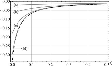
In Section 2, we consider the one-dimensional effective potential, to which the anisotropic Coulomb law gives rise, and which is involved in the one-dimensional Schrödinger equation occurring in the adiabatic approximation of [5]. It is illustrated in Figure 1 how the potental-distance curves condense towards a certain limiting curve for large magnetic fields instead of dropping down infinitely, unlike is the case in QM. The form of the limiting curve predetermines the finiteness of the lower energy levels (as a matter of fact, of all excited levels, as well), which is found in Section 2 using the KP method. Numerical results and the resulting saturation pattern, shown in Figure 4 for the first even-energy levels, are discussed in Section 3.
In this work, we consider the four-dimensional Minkowski space-time, parameterized by coordinates and metric tensor . The electromagnetic field strength tensor and its dual are related through the Levi–Civita antisymmetric tensor, normalized as . The Gaussian system of units, in which , is employed throughout the text.
2 Spectrum Equation for Lower Even-Energy Levels
2.1 Preliminaries
In a constant and homogeneous magnetic field background , the potential generated by a stationary point-like charge distribution , far from it takes the form of anisotropic Coulomb potential [28, 30, 31, 32]
| (1) |
where and are dielectric permittivities, perpendicular to the external field and parallel to it, respectively, and . These are functions of the background magnetic field444The above expression must be understood in a special reference frame where the background is purely magnetic and where the charge distribution is at rest. Such a frame always exists, provided that the first field invariant is positive and the second identically zero.. As the field of the charge in the remote region is slowly varying, these dielectric permittivities are given by the entities associated with quantum electrodynamics taken in the local field approximation (LCFA), i.e., the one whose effective action is local in the sense that its Lagrangian is a function of the field invariants only (and not of space-time derivatives of them). Namely, the permittivities are expressed as and in terms of the derivatives of the local Lagrangian
| (2) |
Because the background is purely magnetic, the above coefficients must be evaluated at after the partial differentiations. For our purposes, the one-loop approximation of the local Lagrangian , known as the Heisenberg–Euler Lagrangian [26, 33], is fitting. However, it is important to note that Equation (1) cannot be blindly extrapolated onto the close vicinity of the charge, where a Yukawa-like form of the potential (thus, quite distinct from (1)) was found beyond the local approximation in [1, 2, 16].
The leading large-field asymptotic behavior for the dielectric permittivities is
| (3) |
where , is the critical Schwinger field, and are the electron charge and mass, and . It is this form that corresponds to the large-field behavior found in [14, 15, 13, 12] for the polarization tensor and exploited in [1, 2], while studying the saturation phenomenon. We shall be basing this on the same Equation (3) in the course of the present study of the saturation within LCFA.
The following reservation is in order, however. The next-to-leading terms of the permittivities can be written with the help of the results in [27] expressed in terms of Hurwitz Zeta functions as follows [28, 34, 35, 36, 37, 38, 39]:
| (4) |
Here, denotes the Psi function [40], which in the large-field limit acquires the asymptotic form
where denotes the Euler constant [40]. The logarithmic contribution into may become essential under such magnetic fields that the value becomes a valuable portion of unity, say , i.e., . The saturation phenomenon we are going to consider here would be violated for those large fields, but there is an important reason to refrain from including them into consideration. The point is that the logarithmic large-field terms in the VP are known [41, 42] to be associated with the logarithmic large-momentum behavior that carries the Fradkin–Landau–Pomeranchuk trouble [43, 44, 45] (also known as the lack of asymptotic freedom) insurmountable within QED. In the present context, the logarithmic term , if taken seriously, would make the transverse dielectric permittivity negative at exponentially large fields, which violates the causality, as discussed in [30]. These conditions supply us with enough arguments to ignore next-to-leading terms resulting from the large-field regime. Therefore, our working range of magnetic fields is
| (5) |
Note that these fields are smaller than/or of the order of the ones, whose magnetic radius, expressed in terms of the electron Compton length as , is of the order of/or smaller than the electromagnetic radius of the proton [46], so that the consideration of the hydrogen atom might retain sense up to . Hence, no new restriction on the range (5) is produced.
Now we are in a position to explain preliminarily how the large screening due to the linear growth of the longitudinal dielectric permittivity (3) in the field range , which fits the range (5), is expected to provide finiteness of the ground-state energy within LCFA. To this end, let us try to extrapolate (3) taken in this regime as close to the charge as possible. The smallest transverse size of the electron Landau orbit in the Hydrogen atom in a strong magnetic field is. Substituting this value for into (3), we obtain the potential
| (6) |
If it were not for the radiative corrections, we would have and this potential in the large field limit would be the singular Coulomb one , since . With such a singularity, the one-dimensional Schrödinger equation governing the degree of freedom parallel to the magnetic field yields an unlimitedly deep energy level according to [3, 4]. On the contrary, with the linearly growing longitudinal dielectric permittivity , the potential, as a function of the longitudinal coordinate, remains ever-finite
This excludes unrestrictedness of the energy level. Moreover, this fact may justify the performed extrapolation of the potential into the short-range domain, where only the polarization tensor beyond LCFA is expected to be valid. To forestall our result for the ground state energy, we note that, numerically, it closely coincides with the value calculated in [19] beyond LCFA, where the large screening provides the saturation via a different mechanism. Namely, it replaces the Coulomb singularity by the Dirac delta-function [1, 2], to which the Yukawa potential turns in the limit .
2.2 Non-Relativistic Wave Equations, Diagonal Approximation and Effective Potential
The nonrelativistic electron in the modified Coulomb field plus a constant magnetic field will be described here by the Pauli Hamiltonian ,
| (7) |
where , are Pauli matrices, is the electron mass and its charge, in absolute value. The Hamiltonian describes the electron motion and its interaction with the external magnetic field
| (8) |
where and denotes the ordinary angular momentum and spin operators, respectively. Because of its cylindric symmetry, splits into two parts , longitudinal, and transverse, , with respect to (positively oriented along the -axis from now on, ). is the Landau Hamiltonian describing the motion on the plane, whose eigenvalues and eigenvectors are and , respectively. Here, and are polar variables while eigen-spinors of , , , . The quantum number corresponds to eigenvalues of the projection of the angular momentum operator on the -axis while to the radial quantum number resulting from the transverse motion, respectively. The explicit form of the radial functions reads
in which denotes the confluent hypergeometric function (CHF) [47].
We are primarily interested in the lower state energies of the stationary Schrödinger equation
| (9) |
specialized to cases where can be treated as a perturbation over the magnetic background. It is noteworthy that even in the approximation where VP is ignored, the problem cannot be straightforwardly solved because the spherical symmetry of the ordinary Coulomb field and the cylindrical symmetry from the magnetic field compete with one another, preventing a complete separation of variables of the Hamiltonian (7) for magnetic fields of arbitrary strength; see, e.g., Refs. [48, 49], and pertinent references therein. For sufficiently strong magnetic backgrounds, the usual approach to the problem consists of expanding the wave function in Landau states
| (10) |
where are expansion functions to be determined. For convenience of notations, we henceforward use for the longitudinal coordinate, . Plugging the expansion (10) into Equation (9) and using the orthogonality of the Landau states, the expansion functions are found to be solutions of the system of differential equations
| (11) |
provided the binding energies , and are related as
| (12) |
and —the effective potential [5, 6, 48] —is defined as
| (13) |
It should be noted that the effective potential is diagonal in the spinning and angular-momentum quantum numbers
| (14) |
on account of the commutativity between , , and .
In general, Equation (11) is a coupled system of differential equations for the functions and the binding energies which can be treated numerically using Hartree–Fock methods, for instance [48]. However, restricting the consideration to strong magnetic fields supplies us with the possibility of treating Equation (11) analytically within the adiabatic approximation [5], in which one neglects contributions from non-diagonal elements of the effective potential , reducing the wave function (10) to and the system (11) to the one-dimensional motion
| (15) |
see, e.g., Refs. [20, 21, 22, 48, 50, 51, 52, 53, 54, 55]. This approximation has been scrutinized over the years, in particular, it was numerically established that it becomes sufficiently accurate for magnetic fields satisfying , where is a reference magnetic field strength for atomic systems555The reference magnetic field is chosen such that the corresponding oscillator energy equals the Rydberg energy . [51, 48, 52]. Rephrasing this condition in terms of the ratio , it corresponds to . This condition is met within our working range (5).
To estimate the energy of lower levels (more precisely, the lowest Landau level band (LLL), specified by , ), we first note that the wave functions are either even or odd with respect to owing to the symmetry of (1) under space reflection, . Hence, we follow the procedure proposed by Karnakov and Popov (KP) to obtain a spectrum equation for even levels [20, 21, 22], which consists of solving the problem in three steps: first at short distances, where Equation (15) can be solved perturbatively, second at sufficiently large distances, where it is exactly solvable, and third equating the logarithmic derivative of the solutions at the overlapping region. To this aim, we first calculate the corresponding effective potentials which, according to Equation (14), are confluent hypergeometric functions [47],
| (16) |
For the purposes of the present work, the permittivities and will be understood mostly as their leading asymptotic limit (3). We find it useful, however, to keep them explicitly for completeness in equations below. From asymptotic properties of CHF with large argument and limiting values as [40], the effective potentials (16) are Coulombian at large distances
| (17) |
and regular at the origin,
| (18) |
whose minimum corresponds to the lowest value for , . This value is finite and, up to a numerical factor, is in agreement with the potential (6) taken in . Moreover, the effective potential curves (16) condense towards the prescribed curve,
| (19) |
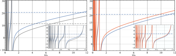
as the magnetic field grows. To see this, note that in the range of magnetic fields under consideration, the asymptotic behavior of the dielectric permittivities (4) is given by Equation (3). In cases where VP is ignored [20, 21, 22], the effective potentials do not condense, and their minima decrease indefinitely as the magnetic field grows, as can be seen from Equation (18) by setting . For illustrative purposes, we present in Figure 1 the effective potentials (16) (with ) for some values of the external field and its corresponding saturation curve, given by Equation (19). Moreover, we supply the first picture with curves corresponding to different values of but a fixed value of the external field, (). This is illustrated by the left panel of Figure 2. In the right panel, we compare the potentials (16) (color solid lines) with the large-distance Coulomb potential (17) (black line) and with potentials whose VP effects are neglected (color dashed lines), Equation (16) with in it.

2.3 Finding the spectrum
Now we are in a position to consider the Schrödinger equation at short distances (with sufficiently small). Following [6, 20, 21, 22], we seek for a perturbative solution in the so-called shallow-well approximation, which can be applied whenever the effective potentials are sufficiently “shallow” according to the condition
| (20) |
This approximation was first considered in one-dimensional problems of quantum mechanics [6], in which stands for the support of the potential well. Because the extent of the effective potential (16) is infinite, it is necessary to choose an appropriately small value to such that the potential be sufficiently shallow according to (20), but also such that for the potential (16) might be considered Coulombian (17) with sufficiently high accuracy. We assume here that the condition (20) is satisfied and postpone the discussion about its validity to the next Section 3, where numerical calculations are discussed in detail.
At this point, it is important to mention that for every pair of quantum numbers , there is an infinite number of longitudinal quantum numbers labeling the longitudinal states666Hereafter, we drop the label from the wave functions for simplicity. such that a complete description of states and energy shifts is given by the set of quantum numbers . Thus, performing a change of variables , , Equation (15) for the LLL reads
| (21) |
where is the Rydberg energy and . In view of the condition (20) and the restriction to even levels, the wave function of longitudinal states varies slowly within the interval (.) and the ground-state binding energies are negligible in comparison to the potential, for . As a result, one can integrate Equation (21) to show that the logarithmic derivative has the form
| (22) |
To obtain Equation (22), we used the boundary conditions , and the approximation
| (23) |
provided . This condition, which will be clarified in the next section, is met for magnetic fields within the range (5) and for larger than the characteristic length of the transverse motion777The dominant contribution to the integral over in (22) comes from values beneath the Landau radius , due to the exponential damping from the wave functions .. As for large distances, one can substitute the approximation (17) into Equation (21) to obtain a Schrödinger equation with one-dimensional Coulomb-like potential [3, 4, 20, 21, 22]. The corresponding solution regular at infinity is the Whittaker function , in which . For sufficiently small arguments, such a solution behaves according to Equation (3.5’) in Ref. [22] (see also Equation (13.14.17) in [40]). Computing the corresponding derivative, we obtain the following approximate expression for the logarithmic derivative,
| (24) |
Matching Equations (22) and (24) we obtain a modified KP equation for even levels888Apart from the usual gauge invariance of the eigenvalues of the Schrödinger equation with external potentials, it is worth noticing that this symmetry is preserved in Equation (25), since the dielectric permittivities depend only on field intensities, and, besides, they are obtained from the gauge-invariant (4-transverse) polarization tensor, like in [1, 2, 7, 8, 9, 10, 11, 12, 30, 56].
| (25) |
The above equation coincides with the KP equation in the regime without radiative corrections.
3 Results
To justify the spectrum equation for the lowest energy levels, we must ascertain whether the conditions under which the approximations considered before are satisfied. More precisely, the modified KP equation (25) relies on the assumption that the shallow-well condition (20) is satisfied at small distances and the fact that the effective potential is Coulombian at large distances (17), with sufficiently high accuracy.
Now, we proceed to study the shallow-well condition (20), as a function of the magnetic field and the distance from the origin, assuming fixed values for . Letting , with an arbitrary positive number, we conveniently rewrite the left-hand side of the condition (20) as
| (26) |
Choosing and using Equation (4), one can calculate the coefficient numerically to conclude that for weaker fields while for stronger fields, admitting distances within the interval . As for larger supports, say , the condition (20) is preserved for weaker fields but violated for strong fields, since , assuming . The condition (20) is improved as grows since the larger the , the shallower the effective potential. For example, and , assuming . Increasing the support to , we find and for . Based on these results, we conclude that there is a range of values to for which the condition (20) is fulfilled for all values of the magnetic field under consideration. Next, one has to verify to what extent the effective potential (16) is Coulombian (17) for slightly larger than . This can be done, for example, analyzing the ratio for several choices of and . Because the CHF is a monotonically increasing function of , the inequality holds for each fixed choice of . Thus, selecting for example, we calculate the ratio and conclude that the effective potential (16) is Coulombian (17) with an accuracy no less than . Moreover, the accuracy decreases as increases999This is not unexpected, because the shallower the effective potential, the more it “deviates” from the Coulombian pattern at small distances, as can be seen in Figure 2., for instance , , . At , we obtain , , , and . Finally, it remains to justify the approximation for the logarithmic derivative of the wave function at small distances, given by Equation (22). This expression relies on the assumption that is satisfied for distances within the short-range interval. To check it, we replace by the magnetic length , , and substitute by its highest value within , i.e., . For , the above parameter varies approximately from to , for magnetic fields within the range (5). As a result, there are no restrictions on the applicability of the approximation (23) in the estimate (22).
Based on these results, we conclude that the modified KP equation (25) meets the requirements needed to estimate energies for lower even levels. To estimate the energies numerically, we conveniently represent the transcendental Equation (25) graphically for some fixed values of the external field and of the quantum number . This is illustrated in Figure 3, where solid lines represent the right-hand side of Equation (25), while the horizontal dashed lines represent the left-hand side, i.e., . For a given set of values to and , one obtains an infinite number of roots of Equation (25) for , but single roots for , corresponding to the deep energy levels; the deepest one owing to , as can be seen on the right panel of Figure 3.
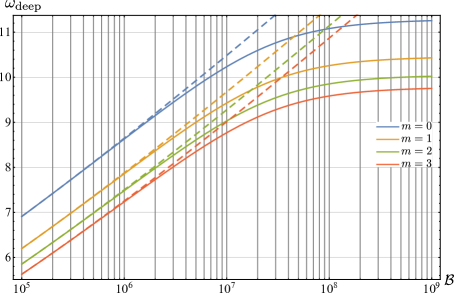
In Figure 4, we illustrate numerical results for the deeper lower energy levels as functions of the magnetic background according to Equation (25) (solid lines). In this same figure, we also include numerical results using the Karnakov–Popov equation without the vacuum polarization (dashed lines).
In contrast to cases where VP is neglected, we observe from Figure 4 that the energy levels “saturate” to specific values as the magnetic field grows. The saturation occurring at sufficiently strong magnetic fields can be computed directly from Equation (25) after the asymptotic expressions for the longitudinal dielectric permittivity (3) are substituted into (25)
| (27) |
The above expression surprisingly coincides with the modified KP equation obtained beyond the local approximation, reported previously by Machet and Vysotsky in [19]. This explains why saturation values obtained within the local approximation
| (28) |
coincide with results obtained in that work. The corresponding saturation energies read , , , and . An explanation for the similarity between our results and those beyond the local approximation can be provided by analyzing the behavior of the logarithmic derivative of the wave functions at short distances. In fact, substituting the Yukawa-like potential101010to which the Coulomb potential is modified by the VP beyond the local approximation [1, 2, 16] in the form it acquires with the help of the interpolation of [19]. in the definition of the effective potential (13) and performing the same approximations as the ones described in the previous section, the authors of [19] found the following expression for the logarithmic derivative
| (29) |
which coincides with our result Equation (22) in the limit of strong magnetic field, thanks to the asymptotic properties of the dielectric permittivities in this case (3). According to these results, we conclude that the saturation of energy levels of the hydrogen atom—known to exist when the atom is exposed to a sufficiently strong magnetic field [1, 2, 19]—can also be obtained within the local approximation.
4 Conclusions
The linear growth of the polarization tensor with the external magnetic field [14, 15, 13, 12, 27] results in strong screening of the static field of a point-like electric charge [1, 2]. It affects the one-dimensional Schrödinger equation responsible for the longitudinal motion of an electron in a hydrogen atom placed in a very strong magnetic field. As a result, the Coulomb singularity close to the charge is deformed. When the polarization tensor is calculated [7, 8, 9, 10, 11] as one loop of electron propagators taken for Green functions of the Dirac equation in a magnetic field, the above behavior is replaced by a Yukawa-like one [1, 2, 16], which turns into as the magnetic field tends to infinity. Contrary to the singularity that leads to an infinite sinking of the ground state energy in that limit, known in quantum mechanics [3, 4], the delta function appearing due to the radiative corrections leaves the ground state energy finite [1, 2]. This is called “saturation” or “freezing” of the level. Its specific value was estimated differently in [1, 2] and in [19, 21, 22]. The latter authors used the “KP method” developed previously in [20] to find the hydrogen spectrum in a strong magnetic field, which improves the calculational results of QM relying on pure adiabatic approximation, when only the diagonal part of the matrix effective potential is used. In applying this method to QED, a simplified interpolation of the polarization tensor was exploited in [19] that allowed to perform analytical calculations to determine large-field asymptotic value of the ground state (as well as excited states), different from the value found in [1, 2] by a different method.
In the present paper, we establish that another approximation for the polarization operator—physically meaningful, contrary to the interpolation of [19]—can be used analytically following the same KP method, that also leads to the saturation.
This is just the Euler–Heisenberg [26] local action approximation LCFA, from which the polarization tensor covering the screening of slowly-varying fields is obtained by differentiations over its field arguments. The asymptotic long-range behavior of the potential (1) of a point-like charge and the corresponding transverse and longitudinal dielectric permittivities , are determined by eigenvalues of this polarization tensor. Their leading large-field asymptotes are given in (3). Similarly to the fact known beyond LCFA, the growth, linear with the magnetic field, is peculiar to the polarization tensor within this approximation and shows itself as the growth of the longitudinal dielectric permittivity in (3) responsible for a growing screening of the charge. The mechanism of how this large screening results in finiteness of the ground-state energy is, however, different within LCFA. It reduces to the change of the minimum size of the wave function, the magnetic length —that in QM tends to zero when increases and thereby supplies the infinity to the potential of the point charge—by the value that has a finite limit . This finite limit makes a sort of elementary length, such that the electron cannot approach the nucleus closer than it. Therefore, the Coulomb singularity is regularized (see (6) or (16)), and the LCFA is better justified. Our final result for the ground state turns out to be the same as beyond this approximation.
Last, but not least, one ought to say that this nontrivial congruence—between results obtained within and beyond the local approximation—can be observed on other physical problems. For example, recently, the running of the fine-structure constant and the electron dynamical mass in a constant magnetic field has been considered beyond the local approximation in [56]. The final reported results for the fine-structure constant for magnetic fields within the range (5) can be equally obtained within the local approximation because the eigenvalue of the polarization tensor in the infrared approximation [30] behaves asymptotically according to Equation (3), capturing thereby the same results of Ref. [56]. As a result, the electron dynamical mass calculated within or beyond the local approximation remains the same.
Acknowledgments
This research was funded by the Russian Science Foundation, grant number 19-12-00042.
References
- [1] Shabad, A.E.; Usov, V.V. Modified Coulomb Law in a Strongly Magnetized Vacuum. Phys. Rev. Lett. 2007, 98, 180403.
- [2] Shabad, A.E.; Usov, V.V. Electric field of a pointlike charge in a strong magnetic field and ground state of a hydrogenlike atom. Phys. Rev. D 2008, 77, 025001.
- [3] Loudon, R. One-Dimensional Hydrogen Atom. Am. J. Phys. 1959, 27, 649.
- [4] Elliot, R.J.; Loudon, R.J. Theory of the absorption edge in semiconductors in a high magnetic field. J. Phys. Chem. Solids 1960, 15, 196.
- [5] Schiff, L.I.; Snyder, H. Theory of the Quadratic Zeeman Effect. Phys. Rev. 1939, 55, 59.
- [6] Landau, L.D.; Lifshits, E.M. Quantum Mechanics; Pergamon Press: Oxford, UK, 1991.
- [7] Batalin, I.A.; Shabad, A.E. Photon green function in a stationary homogeneous field of the most general form. Zh. Eksp. Teor. Fiz. 1971, 60, 894.
- [8] Shabad, A.E. Cyclotronic resonance in the vacuum polarization. Lett. Nuovo Cimento 1972, 3, 457.
- [9] Tsai, W.Y. Vacuum polarization in homogeneous magnetic fields. Phys. Rev. D. 1974, 10, 2699.
- [10] Baier, V.N.; Katkov, V.M.; Strakhovenko, V.M. Operator approach to quantum electrodynamics in an external field. Electron loops. ZhETF 1975, 68, 403.
- [11] Shabad, A.E. Photon dispersion in a strong magnetic field. Ann. Phys. (N.Y.) 1975, 90, 166.
- [12] Shabad, A.E. Polarization of the Vacuum and a Quantum Relativistic Gas in an External Field; Nova Science Publishers: New York, NY, USA, 1991.
- [13] Melrose, D.B.; Stoneham, R.J. Vacuum polarization and photon propagation in a magnetic field. Nuovo Cimento 1977 32, 435.
- [14] Skobelev, V.V. Polarization operator of a photon in a superhigh magnetic field. Izv. Vissh. Uchebn. Zav. Fiz. (Sov. Phys. J.) 1975, 10, 142.
- [15] Loskutov, Y.M.; Skobelev, V.V. Nonlinear electrodynamics in a superstrong magnetic field. Phys. Lett. A 1976, 56, 151.
- [16] Sadooghi, N.; Jalili, A.S. New look at the modified Coulomb potential in a strong magnetic field. Phys. Rev. D 2007, 76, 065013.
- [17] Erber, N. High-Energy Electromagnetic Conversion Processes in Intense Magnetic Fields. Rev. Mod. Phys. 1966, 38, 626.
- [18] Bialyniska-Birula, Z.; Bialyniski-Birula, I. Nonlinear Effects in Quantum Electrodynamics. Photon Propagation and Photon Splitting in an External Field. Phys. Rev. D 1970, 2, 2341.
- [19] Machet, B.; Vysotsky, M.I. Modification of Coulomb law and energy levels of the hydrogen atom in a superstrong magnetic field. Phys. Rev. D 2011, 83, 025022.
- [20] Karnakov, B.M.; Popov, V.S. A hydrogen atom in a superstrong magnetic field and the Zeldovich effect. J. Exp. Theor. Phys. 2003, 97, 890.
- [21] Popov, V.S.; Karnakov, B.M. On the spectrum of the hydrogen atom in an ultrastrong magnetic field. J. Exp. Theor. Phys. 2012, 114, 1.
- [22] Popov, V.S.; Karnakov, B.M. Hydrogen atom in a strong magnetic field. Phys. Usp. 2014, 57, 257.
- [23] Godunov, S.I.; Vysotsky, M.I. Dependence of the atomic energy levels on a superstrong magnetic field with account of a finite nucleus radius and mass. Phys. Rev. D 2013, 87, 124035.
- [24] Greiner, W.; Reinhardt, J. Quantum Electrodynamics; Springer: Berlin, Germany, 1992.
- [25] Oraevskii, V.N.; Rez, A.I.; Semikoz, V.B. Spontaneous production of positrons by a Coulomb center in a homogeneous magnetic field. Zh. Eksp. Teor. Fiz. 1977, 72, 820.
- [26] Heisenberg, W.; Euler, H. Folgerungen aus der Diracschen Theorie des Positrons. Z. Phys. 1936, 98, 714.
- [27] Heyl, J.S.; Hernquist, L. Birefringence and dichroism of the QED vacuum. J. Phys. A 1997, 30, 6485.
- [28] Adorno, T.C.; Gitman, D.M.; Shabad, A.E. Coulomb field in a constant electromagnetic background. Phys. Rev. D 2016, 93, 125031.
- [29] Ritus, V.I. Issues in Intense-Field Quantum Electrodynamics; Nova Science Publ.: New York, NY, USA, 1987.
- [30] Shabad, A.E.; Usov, V.V. Effective Lagrangian in nonlinear electrodynamics and its properties of causality and unitarity. Phys. Rev. D 2011, 83, 105006.
- [31] Villalba-Chávez, S.; Shabad, A.E. QED with an external field: Hamiltonian treatment of Lorentz-non-invariant background as an anisotropic medium. Phys. Rev. D 2012, 86, 105040.
- [32] Gitman, D.M.; Shabad, A.E. Nonlinear (magnetic) correction to the field of a static charge in an external field. Phys. Rev. D 2012, 86, 125028.
- [33] Schwinger, S. On Gauge Invariance and Vacuum Polarization. Phys. Rev. 1951, 82, 664.
- [34] Dittrich, W.; Reuter, M. Effective Lagrangians in Quantum Electrodynamics; Lecture Notes in Physics; Springer: Berlin, Germany, 1985.
- [35] Dittrich, W.; Gies, H. Probing the Quantum Vacuum, Perturbative Effective Action Approach in Quantum Electrodynamics and its Applications; Springer Tracts in Modern Physics; Springer: Berlin, Germany, 2000.
- [36] Elizalde, E. Ten Physical Applications of Spectral Zeta Functions, 2nd ed.; Lecture Notes in Physics; Springer: Berlin/Heidelberg, Germany, 2012; Volume 855.
- [37] Kirsten, K. Spectral Functions in Mathematics and Physics; Chapman & Hall/CRC: Boca Raton, FL, USA, 2002.
- [38] Dunne, G.V. From Fields to Strings: Circumnavigating Theoretical Physics; Shifman, M., Vainshtein, A., Wheater, J., Eds.; World Scientific: Singapore, 2005; pp. 445–522.
- [39] Karbstein, F.; Shaisultanov, R. Photon propagation in slowly varying inhomogeneous electromagnetic fields. Phys. Rev. D 2015, 91, 085027.
- [40] Olver, F.W.J.; Lozier, D.W.; Boisvert, R.F.; Clark, C.W. NIST Handbook of Mathematical Functions; Cambridge University Press: New York, NY, USA, 2010.
- [41] Ritus, V.I. Lagrangian of an intense electromagnetic field and quantum electrodynamics at short distances. Zh. Eksp. Teor. Fiz. 1975, 69, 1517.
- [42] Ritus, V.I. Connection between strong-field quantum electrodynamics with short-distance quantum electrodynamics. Zh. Eksp. Teor. Fiz. 1977, 73, 807.
- [43] Landau, L.D.; Pomeranchuk, Y.I. On Point Interactions in Quantum Electrodynamics. Dokl. Akad. Nauk SSSR 1955, 102, 489.
- [44] Pomeranchuk, Y.I. Zero equality of renormalized charge in quantum electrodynamics. Dokl. Akad. Nauk SSSR 1955, 103, 1005.
- [45] Fradkin, E.S. The Asymptote of Green’s Function in Quantum Electrodynamics. Zh. Eksp. Teor. Fiz. 1955, 28, 750.
- [46] The NIST Reference on Constants, Units, and Uncertainty. Available online: https://physics.nist.gov/cuu/Constants/index.html (accessed on September, 2020.).
- [47] Erdélyi, A. Higher Transcendental Functions; Bateman Manuscript Project; MacGraw-Hill: New York, NY, USA, 1953; Volume 1.
- [48] Ruder, H.; Wunner, G.; Herold, H.; Geyer, F. Atoms in Strong Magnetic Fields—Quantum Mechanical Treatment and Applications in Astrophysics and Quantum Chaos; Springer: Berlin, Germany, 1994.
- [49] Friedrich, H.; Wintgen, D. The hydrogen atom in a uniform magnetic field—An example of chaos. Phys. Rep. 1989, 183, 37.
- [50] Simola, J.; Virtamo, J. Energy levels of hydrogen atoms in a strong magnetic field. J. Phys. B At. Mol. Phys. 1978, 11, 3309.
- [51] Wunner, G.; Ruder, H. Lyman- and Balmer-like transitions for the hydrogen atom in strong magnetic fields. Astron. Astrophys. 1980, 89, 241.
- [52] Wunner, G.; Ruder, H. Electromagnetic transitions for the hydrogen atom in strong magnetic fields. Astrophys. J. 1980, 242, 828.
- [53] Wunner, G.; Ruder, H.; Herold, A. Quality of one-configuration hartree-fock-type calculations for the H atom in arbitrary magnetic fields. Phys. Lett. A 1981, 85, 430.
- [54] Friedrich, H. Bound-state spectrum of the hydrogen atom in strong magnetic fields. Phys. Rev. A 1982, 26, 1827.
- [55] Rösner, W.; Herold, H.; Ruder, H.; Wunner, G. Approximate solution of the strongly magnetized hydrogenic problem with the use of an asymptotic property. Phys. Rev. A 1983, 28, 2071.
- [56] Ferrer, E.J.; Sanchez, A. Magnetic field effect in the fine-structure constant and electron dynamical mass. Phys. Rev. D 2019, 100, 096006.