PeleNet: A Reservoir Computing Framework for Loihi

Abstract

High-level frameworks for spiking neural networks are a key factor for fast prototyping and efficient development of complex algorithms. Such frameworks have emerged in the last years for traditional computers, but programming neuromorphic hardware is still a challenge. Often low level programming with knowledge about the hardware of the neuromorphic chip is required. The PeleNet framework aims to simplify reservoir computing for the neuromorphic hardware Loihi. It is build on top of the NxSDK from Intel and is written in Python. The framework manages weight matrices, parameters and probes. In particular, it provides an automatic and efficient distribution of networks over several cores and chips. With this, the user is not confronted with technical details and can concentrate on experiments.

Note: This is a draft

Introduction

Several different neuromorphic hardware chips have been developed in recent years (reviewed by Schuman et al., 2017; Young et al., 2019; Rajendran et al., 2019). All of them promise to be a key factor in future neuroscientific research as well as technological developments in artificial intelligence. The main benefit of neuromorphic systems is their low power consumption and speed (Rajendran et al., 2019). Shown for Loihi for example from Tang et al. (2019). This advantage of brain inspired hardware comes with a solution to the von Neumann bottleneck (Backus, 1978). While novel neuromorphic hardware becomes more and more powerful, algorithms for such hardware systems are still in an early stage. A specific field of spiking neural network algorithms, which can be used for neuromorphic hardware, is reservoir computing. For details about reservoir computing I refer the reader to the literature (Jaeger, 2001; Maass et al., 2002; Jaeger, 2007; Schrauwen et al., 2007; Lukoševičius et al., 2012; Goodfellow et al., 2016).

Here, I focus on the neuromorphic hardware chip Loihi (Davies et al., 2018). The chip is digital and includes a current-based (CUBA) leaky integrate-and-fire (LIF) neuron. A chip contains $128$ cores and each core time-multiplexes $1024$ compartments. In addition, every chip contains three conventional x86 CPUs. Several chips can be used in parallel on one board. The parameters of the synapses and the compartments can be adapted, but the neuron model itself is fixed. A single compartment neuron can be extended to a multi compartment neuron which comes with the cost of less available neurons. Intel provides a software development kit, the so-called NxSDK which is written in Python and already allows higher-level programming of the chip (Lin et al., 2018). In addition, C scripts can be used to run code on the x86 CPUs of the chip. The NxSDK allows to define compartment prototypes and compartment groups which can be combined to neuron prototypes and neurons. Using connection prototypes and connections these compartments and neurons can be interconnected using a connection matrix. Spikes can be injected using spike generators and several different types of probes can be defined. Finally, learning rules can be used to make connections in the reservoir plastic.

However, the NxSDK defines compartments for each core separately. If bigger networks are used, it is necessary to split the connections manually to the Loihi cores. Compartments between cores need then to be interconnected manually, which results in $n_{\text{conn}}=n_{\text{core}}^{2}$ connection matrices, if all potential connections should be possible. For example, if we create $3$ compartment groups, distributed to $n_{\text{core}}=3$ cores, and we want to interconnect all of them, we need to define $n_{\text{conn}}=9$ connection weight matrices, which is illustrated in Figure 1B. Note that this amount of matrices is necessary even for sparse reservoirs networks, since we do not want to exclude any possibility a priori. In addition to handling these connection matrices, also probes can only be taken for each core individually. Probing the whole network from the example above requires defining and handling $3$ probes for the compartment groups and $9$ probes for the connection weight matrices. Note that this problem is only difficult in recurrent structures, especially in a reservoir where all neurons can potentially connect to each other. In feed-forward structures, even in deep spiking neural networks (already applied to several neuromorphic hardware systems, see e.g. Diehl et al., 2016; Schmitt et al., 2017; Patino-Saucedo et al., 2020; Massa et al., 2020), this problem is less predominant since the layers are connected in series. Multiple probes still need to be defined, but the connection matrices scale linear with the number of neuron groups and not quadratic as in reservoirs.

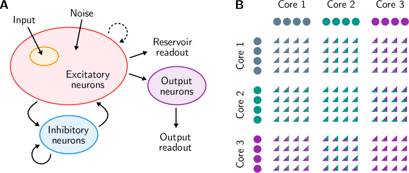
Figure 1: (A) The reservoir network consists of a pool of excitatory neurons (red) and a pool of inhibitory neurons (blue). Those pools are connected within and in-between. The excitatory neurons can be stimulated by an input (orange) and/or noise. Optionally a pool of output neurons (purple) can be defined. The spiking data can be read out from the reservoir itself and/or from the output neurons. PeleNet supports configuring a learning rule for the connections of the excitatory neurons (dotted arrow). (B) The example shows $12$ neurons which are distributed to three cores, where each core contains four neurons. Each core is color coded (grey, green, purple). Every triangle symbolises a potential connection between two neurons. The color of the triangle indicates which cores need to be interconnected to interconnect the related neurons. In this case, neurons spread over three cores require $9$ connection matrices.

The PeleNet framework was developed to solve the distribution of connections efficiently and to make it easy for the user. In the framework, the experimenter only needs to define one connection matrix for every part of the network (e.g. for the reservoir or for the output layer). After the simulation, the user gets usable probes for every part of the network. In addition, PeleNet provides different distributions for initializing the connection weights, defining learning rules, creating standard plots, logging relevant computation steps and a collection of utils for calculating statistics and handling data. Moreover, the framework is a whole new abstraction layer on top of the NxSDK. Compartments, connections and probes are defined implicitly and are controlled via parameters. Due to its modular and object oriented architecture, the framework can easily be extended with additional functionality. Here, I give a brief overview of the code structure and the main features. The code is available on Github under the MIT license.

Design and implementation

Pele is the goddess of volcanoes and fire in the Hawaiian religion (Nimmo, 1986; Emerson, 2013). She has the control over lava and volcanoes and is inter alias in control of the volcano Loihi. The name of the PeleNet framework is an eponym of the goddess Pele.

The framework is build to allow experiments with reservoir networks on Loihi. As shown in Figure 1A, PeleNet currently supports reservoir networks that follow Dale’s law. The reservoir contains a pool of excitatory and a pool of inhibitory neurons. Those neuron pools are connected within and in-between. Additionally an input, noise and an output is available. The spiking data can be read out from the excitatory, inhibitory and output neurons. Every experiment can contain one or multiple trials. Figure 3 shows an example with $10$ trials. The spiking activity can optionally be reset after every trial. With this, it is possible to simulate much faster, since is is not necessary to initialize the network again after every trial.

Programmatically, PeleNet consists of two main parts. One part contains some helper functions and external libraries which are not available as a package. This part is imported from the PeleNet framework internally, the user does not need to import modules from this part. The other part consists of the PeleNet code itself which is imported and used by the user.

Libraries

The lib folder currently contains code to generate an anisotropic connectivity matrix and some helper functions and classes. The code for initializing an anisotropic connectivity matrix is public on Github . The underlying principle was introduced in (Spreizer et al., 2019) and used in (Michaelis et al., 2020) for generating robust robotic trajectories, using the PeleNet framework. The helper folder contains custom exception functions for invalid parameters or invalid function arguments and a Singleton class to decorate classes in the PeleNet framework to make use of the singleton design pattern.

PeleNet structure

The central entity of PeleNet is the experiment, which inherits from an abstract experiment. In an experiment one or several networks can be defined and used. In the experiment, a parameter set is defined and overwrites values of the default parameter object. The parameters are passed to every network, when it is initialized by the experiment. In addition, every network contains a plot object, which has access to the data sets and probes of the simulation. Passing data to one of the plot methods is therefore in most cases not necessary. Hence, the arguments in den plot method shape the plots appropriately in size, limits, labels, colors, etc. Two singleton objects are globally available to all other objects. The system singleton contains a datalog object which logs all important steps in a log file. It also logs the parameter set which was used for a particular experiment and basic plots and optionally data sets from this experiment. The utils singleton provides a bunch of methods to handle and evaluate data, like dimensionality reduction, smoothing, calculating the spectral radius of the weight matrix and different kind of statistics. Figure 2 gives an overview of the dependencies between the classes in PeleNet.

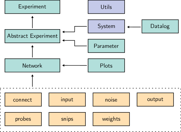
Figure 2: The code structure of the PeleNet framework. Classes have a green background, singletons are in purple and collections of methods for a class are yellow.

Network

The major component of the PeleNet framework is the network. It contains a collection of methods, distributed over several files. Since this is the core of the framework, I will give some more details about the behavior in the following listing.

weights

Methods in the weights file initialize the weight matrices for all parts of the network. The basic weight matrices are for connecting the excitatory and inhibitory parts of the reservoir. Weights can be initialized using constant values or a log-normal or normal distribution. In addition, a 2D topological anisotropic weight matrix can be initialized. All weight matrices are stored sparsely in a compressed sparse row (CSR) format.

connect

Takes a weight matrix for every part of the network (e.g. one weight matrix for the whole reservoir), splits it in parts (called chunks in the framework), distributes these parts to the cores and interconnects them to each other. It is currently still necessary to define the number of neurons that should be used per core as a parameter. For an efficient distribution we need to consider two aspects. First, every core time-multiplexes up to $1024$ neurons, the less neurons we simulate on every core, the faster the simulation will be. Second, the more cores are used, the more connection matrices are required, which slows down the initialization of the network. For an optimal run-time performance we should therefore reduce the number of neurons per core as much as possible and for an optimal initialization performance we should use as much neurons per core as possible. It is currently up to the user to choose best fitting values for this trade-off, but in most cases it is probably the fast simulation time which is desired. Later versions of the framework may allow the user to choose a preferred method and handles the distribution of neurons automatically.

input

Adds different types of inputs to the network. All of them base on the spike generators from the NxSDK. Currently topological inputs (in case of a 2D-network), noisy inputs (leave-n-neurons out in every trial), sequences of inputs and varying input positions per trial are supported. Topological inputs define a square of stimulated neurons in the excitatory layer of the reservoir at a defined position. Noisy inputs stimulate a specific number of reservoir neurons, but in every trial some few neurons are left out such that the input differs slightly in every trial. A sequence of inputs are multiple input regions which are stimulated in a row within one trial such that relations between them can be learned (e.g. with spike-timing-dependent plasticity). An example for a input sequence is shown in Figure 3. Finally, it is possible to define separate input regions, where one input region is randomly chosen in every trial.

noise

Noise is currently generated by random inputs from spike generators which are connected to randomly chosen neurons in the network. Future implementations will probably make use of random changes in the current of a synapse or the membrane voltage of the neuron.

output

Adds output neurons to the reservoir. Currently the only available output is a pooling layer, which was used in Michaelis et al. (2020). The pooling layer was used for a faster read out and performed regularization for the anisotropic network.

probes

Contains several methods to define and process probes. First, probes are defined for every core and every connection matrix chunk. Second, after a successful simulation, probe data are post-processed and stacked together to complete and useful data sets. Note that the output of a connection weight probes is in CSR format again such that this matrix can directly be used as an initial connection matrix for another simulation.

snips

Handles small C-scripts that run on the x86 cores of the Loihi chips (so called SNIPs). These scripts are located in the pelenet/snips folder. Currently a reset SNIP is available that resets the membrane voltages after a trial. It is important to note that the plasticity is currently not stopped while resetting the membrane voltages, which can cause problems when the $uk$ variables ares used. But this feature is under development and will probably be added soon.

⬇

1# Import abstract experiment

2from ._abstract import Experiment

3

4”””

5@desc: An experiment with a sequential input, trained over several trials

6”””

7class SequenceExperiment(Experiment):

8

9 ”””

10 @desc: Define parameters for this experiment

11 ”””

12 def defineParameters(self):

13 return {

14 # Experiment

15 ’seed’: 1, # Set fixed random seed

16 ’trials’: 10, # Number of trials

17 ’stepsPerTrial’: 60, # Number of simulation steps for every trial

18 # Neurons

19 ’refractoryDelay’: 2, # Refactory period

20 ’voltageTau’: 100, # Voltage time constant

21 ’currentTau’: 5, # Current time constant

22 ’thresholdMant’: 1200, # Spiking threshold for membrane potential

23 # Network

24 ’reservoirExSize’: 400, # Number of excitatory neurons

25 ’reservoirConnPerNeuron’: 35, # Number of connections per neuron

26 ’isLearningRule’: True, # Apply a learning rule

27 ’learningRule’: ’2^-2*x1*y0 - 2^-2*y1*x0 + 2^-4*x1*y1*y0 - 2^-3*y0*w*w’,

28 # Input

29 ’inputIsSequence’: True, # Activates sequence input

30 ’inputSequenceSize’: 3, # Number of input clusters in sequence

31 ’inputSteps’: 20, # Number of steps a trace input is active

32 ’inputGenSpikeProb’: 0.8, # Probability of spike for the input generator

33 ’inputNumTargetNeurons’: 40, # Number of neurons activated by the input

34 # Probes

35 ’isExSpikeProbe’: True, # Probe excitatory spikes

36 ’isInSpikeProbe’: True, # Probe inhibitory spikes

37 ’isWeightProbe’: True # Probe weight matrix at the end of every trial

38 }

Listing 1: Defining an experiment in the pelenet/experiments folder. The defineParameters method is required. Lifecycle methods are optional (not shown). In addition, the experiment can be extended by custom methods for e.g. data evaluation or visualization.

Experiments

An experiment inherits from an abstract experiment and is created in the pelenet/experiments folder. The abstract experiment inherits again from the ABC package, which allows defining abstract methods. The defineParameters method in the abstract experiment class is implemented as an abstract method that is then necessary in every experiment, otherwise an exception is thrown. The abstract experiment also provides some default functionality, which can optionally be overwritten. It initializes all necessary objects for the experiment and contains a default build process. Also the execution of the simulation follows a default behavior. In both cases, it is preferred to control the behavior of the experiment via parameters instead of overwriting methods. If the parameters do not cover the wanted behavior, it is suggested to make use of the available lifecycle methods. Available lifecycle methods are:

• onInit: Called after the experiment was initialized.

• afterBuild: Called after all network parts are connected (i.e. weight matrix, inputs, outputs, noise, probes).

• afterRun: Called after the simulation has finished and all data are post-processed.

Only if the parameters and the lifecycle methods are not sufficient to solve the intended behavior it is suggest to overwrite the build and run methods of the abstract experiment.

In practice, Jupyter notebooks are used to quickly evaluate the results of an experiment. It is suggested to use Jupyter notebooks only for visualization of the results and for prototyping. Code for the experiment should be included in the defined experiment. An example of a simple experiment is shown in Code Listing 1. In Code Listing 2 the experiment is used. The plotted spike train from the Code Listing 2 (line $25$) is shown in Figure 3.

Parameters

⬇

1# Load pelenet modules

2from pelenet.experiments.sequence import SequenceExperiment

3

4# Overwrite default parameters from pelenet/experiments/sequence.py

5parameters = {

6 # Experiment

7 ’seed’: 2, # Change random seed

8}

9

10# Initialize experiment

11# The name is optional, it is extended to the folder in the log directory

12# The parameters defined above are handed over to the experiment object

13exp = SequenceExperiment(

14 name=’random-network-sequence-learning’,

15 parameters=parameters

16)

17

18# Build the network (weight matrix, inputs, probes, etc)

19exp.build()

20

21# Run the network simulation, afterwards the probes are post-processed to nice arrays

22exp.run()

23

24# Plot spike trains of the excitatory and inhibitory neurons

25exp.net.plot.reservoirSpikeTrain(figsize=(12,6))

Listing 2: An example for running the experiment. For this Jupyter notebooks can be used. Parameters of the experiment can be overwritten to allow fast experimentation. At the end of the script an included plotting method is called to show spike trains. They are directly plotted in Jupyter and stored in the log folder related to this simulation.

The parameter system is a powerful tool of PeleNet for defining an experiment. All NxSDK functionalities, which are included in PeleNet, are covered by the parameter set. It is not required to know anything about the NxSDK at all, if the functionality provided by PeleNet is sufficient for the user. The default parameters are split in three parts, parameters for the experiment, the system and derived parameters. The system parameters cover information about e.g. the used Loihi board, settings for the matplotlib library, logging and paths. The experiment parameters contain e.g. neurons, connections, inputs, outputs, noise, probes and also a learning rule for the reservoir. Finally, the derived parameters are calculated from the system and experiment parameters and are useful for the framework or for the user. Some parameters are sanity checked to avoid serious issues with false parameters. These checks are constantly extended. Note that the parameters are well documented in the pelenet/parameters file to understand their meaning, but it is not suggested to overwrite the parameters there. For overwriting parameters the defineParameters method is available in the experiment. All parameter values which are defined in this method overwrite the default parameter set. Derived parameters are calculated after the parameters are defined in an experiment.

Discussion

Currently the neuromorphic hardware community grows fast and it is probably only a matter of time until new or updated hardware systems will emerge. The field of applications is very broad for such hardware, including the estimation of linear models, like LASSO (Shapero et al., 2014; Davies et al., 2018), non-parametric classification with k-nearest neighbor (Frady et al., 2020), deep spiking neural network (Massa et al., 2020) or reservoir networks (Michaelis et al., 2020). High-level libraries and frameworks are needed to cover these different specialized application areas. While for deep spiking neural networks the SNN Toolbox (Rueckauer et al., 2017; Rueckauer and Liu, 2018) is available for ANN to SNN conversions (also for Loihi) or SLAYER is available for training SNNs via backpropagation, reservoir network frameworks are still rare for neuromorphic computing.

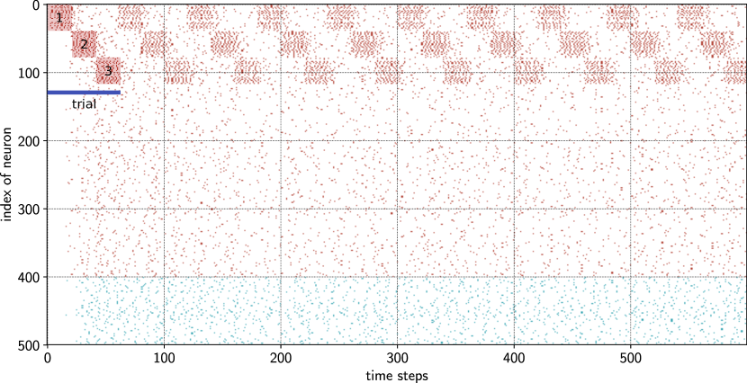
Figure 3: Example for a spike raster plot that shows inputs and trials. The experiment was performed with $10$ trials and a input sequence with three inputs.

The here presented PeleNet framework simplifies the implementation of reservoir networks on the neuromorphic hardware Loihi. The framework is an abstraction layer on top of the NxSDK from Intel. PeleNet allows an efficient distribution of the network over an arbitrary number of Loihi cores and chips. Probes are combined to data sets, which can directly be used for further evaluations. Parameters define the experiments. The “parameter approach” allows an easy initialization process and keeps the experiments clear. Finally, the plot systems already includes a bunch of default plots for reservoir computing.

Beside its already existing features, the framework is still in an early stage. Some functionalities of the Loihi chip are not provided yet. This includes inter alia current and voltage noise, usage of the tag for learning rules and synaptic delays. The learning rule covers the excitatory neurons in the reservoir, future version will also be able to apply a learning rule to output neurons. In addition, the framework is not yet available as a pip python package and still requires a manual installation of dependencies. Therefore one of the next steps will be to provide a package release of PeleNet. It is also intended to add an optimization functionality which runs several experiments in order to find optimal parameters, according to a criterion. The parameter system is already designed to support future optimization scripts. Finally, it is planned to add unit and integration tests to make sure that simulations are performed correctly. Currently four Jupyter notebooks are available as functional tests.

The aim of PeleNet is to speed up the implementation of reservoir computing experiments on Loihi. In a more broad perspective it has even the potential to push the field of reservoir computing implementations on neuromorphic hardware in general. Despite its early development stage, I am confident that the framework is already useful for computational studies.

License and code availability

The framework PeleNet is published under the MIT License and is therefore freely available without warranty. The code is available on Github. Contributions are highly appreciated.

References

- Backus (1978) Backus, J. (1978). Can programming be liberated from the von neumann style? a functional style and its algebra of programs. Commun. ACM, 21(8):613–641.
- Davies et al. (2018) Davies, M., Srinivasa, N., Lin, T.-H., Chinya, G., Cao, Y., Choday, S. H., Dimou, G., Joshi, P., Imam, N., Jain, S., et al. (2018). Loihi: A neuromorphic manycore processor with on-chip learning. IEEE Micro, 38(1):82–99.
- Diehl et al. (2016) Diehl, P. U., Zarrella, G., Cassidy, A., Pedroni, B. U., and Neftci, E. (2016). Conversion of artificial recurrent neural networks to spiking neural networks for low-power neuromorphic hardware. In 2016 IEEE International Conference on Rebooting Computing (ICRC), pages 1–8. IEEE.
- Emerson (2013) Emerson, N. B. (2013). Pele and Hiiaka: a myth from Hawaii. Tuttle Publishing.
- Frady et al. (2020) Frady, E. P., Orchard, G., Florey, D., Imam, N., Liu, R., Mishra, J., Tse, J., Wild, A., Sommer, F. T., and Davies, M. (2020). Neuromorphic nearest neighbor search using intel’s pohoiki springs. In Proceedings of the Neuro-Inspired Computational Elements Workshop, NICE ’20, New York, NY, USA. Association for Computing Machinery.
- Goodfellow et al. (2016) Goodfellow, I., Bengio, Y., and Courville, A. (2016). Deep Learning. MIT Press. http://www.deeplearningbook.org.
- Jaeger (2001) Jaeger, H. (2001). The “echo state” approach to analysing and training recurrent neural networks-with an erratum note. Bonn, Germany: German National Research Center for Information Technology GMD Technical Report, 148(34):13.
- Jaeger (2007) Jaeger, H. (2007). Echo state network. Scholarpedia, 2(9):2330. revision #189893.
- Lin et al. (2018) Lin, C.-K., Wild, A., Chinya, G. N., Cao, Y., Davies, M., Lavery, D. M., and Wang, H. (2018). Programming spiking neural networks on intel’s loihi. Computer, 51(3):52–61.
- Lukoševičius et al. (2012) Lukoševičius, M., Jaeger, H., and Schrauwen, B. (2012). Reservoir computing trends. KI-Künstliche Intelligenz, 26(4):365–371.
- Maass et al. (2002) Maass, W., Natschläger, T., and Markram, H. (2002). Real-time computing without stable states: A new framework for neural computation based on perturbations. Neural computation, 14(11):2531–2560.
- Massa et al. (2020) Massa, R., Marchisio, A., Martina, M., and Shafique, M. (2020). An efficient spiking neural network for recognizing gestures with a dvs camera on the loihi neuromorphic processor. arXiv preprint arXiv:2006.09985.
- Michaelis et al. (2020) Michaelis, C., Lehr, A. B., and Tetzlaff, C. (2020). Robust robotic control on the neuromorphic research chip loihi. arXiv preprint arXiv:2008.11642.
- Nimmo (1986) Nimmo, H. A. (1986). Pele, ancient goddess of contemporary hawaii. Pacific Studies, 9(2):121.
- Patino-Saucedo et al. (2020) Patino-Saucedo, A., Rostro-Gonzalez, H., Serrano-Gotarredona, T., and Linares-Barranco, B. (2020). Event-driven implementation of deep spiking convolutional neural networks for supervised classification using the spinnaker neuromorphic platform. Neural Networks, 121:319–328.
- Rajendran et al. (2019) Rajendran, B., Sebastian, A., Schmuker, M., Srinivasa, N., and Eleftheriou, E. (2019). Low-power neuromorphic hardware for signal processing applications: A review of architectural and system-level design approaches. IEEE Signal Processing Magazine, 36(6):97–110.
- Rueckauer and Liu (2018) Rueckauer, B. and Liu, S.-C. (2018). Conversion of analog to spiking neural networks using sparse temporal coding. In 2018 IEEE International Symposium on Circuits and Systems (ISCAS), pages 1–5. IEEE.
- Rueckauer et al. (2017) Rueckauer, B., Lungu, I.-A., Hu, Y., Pfeiffer, M., and Liu, S.-C. (2017). Conversion of continuous-valued deep networks to efficient event-driven networks for image classification. Frontiers in neuroscience, 11:682.
- Schmitt et al. (2017) Schmitt, S., Klähn, J., Bellec, G., Grübl, A., Guettler, M., Hartel, A., Hartmann, S., Husmann, D., Husmann, K., Jeltsch, S., et al. (2017). Neuromorphic hardware in the loop: Training a deep spiking network on the brainscales wafer-scale system. In 2017 International Joint Conference on Neural Networks (IJCNN), pages 2227–2234. IEEE.
- Schrauwen et al. (2007) Schrauwen, B., Verstraeten, D., and Van Campenhout, J. (2007). An overview of reservoir computing: theory, applications and implementations. In Proceedings of the 15th european symposium on artificial neural networks. p. 471-482 2007, pages 471–482.
- Schuman et al. (2017) Schuman, C. D., Potok, T. E., Patton, R. M., Birdwell, J. D., Dean, M. E., Rose, G. S., and Plank, J. S. (2017). A survey of neuromorphic computing and neural networks in hardware. arXiv preprint arXiv:1705.06963.
- Shapero et al. (2014) Shapero, S., Zhu, M., Hasler, J., and Rozell, C. (2014). Optimal sparse approximation with integrate and fire neurons. International journal of neural systems, 24(05):1440001.
- Spreizer et al. (2019) Spreizer, S., Aertsen, A., and Kumar, A. (2019). From space to time: Spatial inhomogeneities lead to the emergence of spatiotemporal sequences in spiking neuronal networks. PLoS computational biology, 15(10):e1007432.
- Tang et al. (2019) Tang, G., Shah, A., and Michmizos, K. P. (2019). Spiking neural network on neuromorphic hardware for energy-efficient unidimensional slam. arXiv preprint arXiv:1903.02504.
- Young et al. (2019) Young, A. R., Dean, M. E., Plank, J. S., and Rose, G. S. (2019). A review of spiking neuromorphic hardware communication systems. IEEE Access, 7:135606–135620.